Accessing Linearly Polarized Gluon Distribution in $J/\psi$ Production at the Electron-Ion Collider

Abstract

We calculate the $cos~{}2\phi_{h}$ asymmetry in $J/\psi$ production in electron-proton collision for the kinematics of the planned electron-ion collider (EIC). This directly probes the Weiszäcker-Williams (WW) type linearly polarized gluon distribution. Assuming generalized factorization, we calculate the asymmetry at next-to-leading-order (NLO) when the energy fraction of the $J/\psi$ satisfies $z<1$ and the dominating subprocess is $\gamma^{*}+g\rightarrow c+{\bar{c}}+g$. We use non-relativistic QCD based color singlet (CS) model for $J/\psi$ production. We investigate the small $x$ region which will be accessible at the EIC. We present the upper bound of the asymmetry, as well as estimate it using a (i) Gaussian type parametrization for the TMDs and (ii) McLerran-Venugopalan (MV) model at small $x$. We find small but sizable asymmetry in all the three cases.

I Introduction

$J/\psi$ electroproduction is a direct probe of gluon transverse momentum dependent parton distributions (TMDs), as the leading process is the virtual photon-gluon fusion. Very little is known so far about the gluons TMDs Mulders and Rodrigues (2001), apart from a positivity bound. Recently, unpolarized TMD gluon pdfs have been extracted from LHCb data Lansberg et al. (2018). TMD pdfs are process dependent due to the initial and/or final state interactions, in other words, due to the presence of gauge links in their operator definitions. Each gluon TMD contains two gauge links in contrast to the quark TMDs that contain one. Because of this, the process dependence of gluon TMDs is more involved than quark TMDs Buffing et al. (2013). The simplest possible configurations are both future pointing [++] or one future and one past pointing [+-] gauge links. In the literature related to small-$x$ physics, the former is called Weizsäcker-Williams (WW) gluon distribution Kovchegov and Mueller (1998); McLerran and Venugopalan (1999). For unpolarized gluons, WW gluon distribution can be interpreted as the number density of gluons inside hadrons in light-cone gauge. The other distribution, [+-], is called dipole distribution Dominguez et al. (2012). This appears in many physical processes and is the Fourier transform of the color dipole amplitude Iancu et al. (2002); Kharzeev et al. (2003). In small $x$ physics, these two types of unintegrated gluon distributions have been discussed in the literature quite extensively Boer et al. (2016); Dominguez et al. (2011a); Metz and Zhou (2011); Schafer and Zhou (2013); Akcakaya et al. (2013); Dumitru et al. (2015); Marquet et al. (2018); Dominguez et al. (2011b); Boer et al. (2017). Apart from the unpolarized gluon TMD, the linearly polarized gluon TMD recently has attracted quite a lot of interest. This basically measures an interference between an amplitude when the active gluon is polarized along $x$ (or $y$) direction and a complex conjugate amplitude with the gluon polarized in $y$ (or $x$) direction in an unpolarized hadron Dominguez et al. (2012). This was introduced for the first time in Mulders and Rodrigues (2001) and calculated in a model in Meissner et al. (2007). It has been shown that the linearly polarized gluon distribution affect the unpolarized cross section of scattering processes, as well an azimuthal asymmetry of the type $cos2\phi_{h}$ Pisano et al. (2013) . The linearly polarized gluon distribution is a time-reversal even (T even) object, and can be WW type or dipole type, depending on the gauge links. $J/\psi$ production in $ep$ collision probes the WW type linearly polarized gluon TMD through a virtual photon-gluon fusion process. The leading order (LO) process $\gamma^{*}+g\rightarrow c{\bar{c}}\rightarrow J/\psi$ contributes to the asymmetry at $z=1$ Mukherjee and Rajesh (2017a). The linearly polarized gluon distribution has not been extracted from data yet. However, there are quite a large amount of theoretical studies about how to probe it in different experiments. In Boer et al. (2009) the authors have proposed to probe it in dijet imbalance in the unpolarized hadronic collision and also in heavy quark pair production in ep collision and in pp collision Pisano et al. (2013); Marquet et al. (2018); Efremov et al. (2018a, b). It can also be probed in quarkonium pair production in $pp$ collision Lansberg et al. (2018), and in associated production of a dilepton and $J/\psi$ Lansberg et al. (2017). Very recently, in Dumitru et al. (2018) the authors have investigated the possibility to probe it in dijet imbalance in $eA$ collision. $h_{1}^{\perp g}$ affects the transverse momentum distribution of final state hadron like Higgs boson Sun et al. (2011); Boer et al. (2013, 2012); Echevarria et al. (2015) and heavy quarkonium Boer and Pisano (2012); Mukherjee and Rajesh (2017b); Mukherjee and Rajesh (2016) in unpolarized pp collision. Although $h_{1}^{\perp g}$ can be probed in $pp$ and $pA$ collision, initial and final state interactions may affect the factorization in such processes. Such complications are less in $ep$ collision processes for example at the electron-ion collider (EIC). In a previous work Mukherjee and Rajesh (2017a) we have investigated the possibility of probing $h_{1}^{\perp g}$ in $cos~{}2\phi$ asymmetry in $J/\psi$ production through the leading order (LO) process $\gamma^{*}+g\rightarrow J/\psi$ at the future EIC. This $2\rightarrow 1$ process contributes at $z=1$, where $z$ is the energy fraction of the photon carried by the $J/\psi$ in the proton rest frame. Here, we extend our analysis to the kinematical region $z<1$. We consider the unpolarized $eP$ collision. The production mechanism of $J/\psi$ is not yet well-understood theoretically. The most widely used approach is based on non-relativistic QCD (NRQCD) Bodwin et al. (1995). Here one assumes a factorization of the amplitude into a hard part where the $c{\bar{c}}$ pair is produced perturbatively in the process $\gamma^{*}+g\rightarrow c+{\bar{c}}+g$. The heavy quark pair then hadronizes to form the $J/\psi$ bound state. The hadronization is described in terms of the long distance matrix elements (LDMEs) which are obtained by fitting the data. For some LDMEs lattice calculations are available. They have definite scaling properties with respect to the velocity parameter $v$, which is assumed to be small. The cross section for the production of $J/\psi$ is expressed as a double expansion in terms of the strong coupling constant $\alpha_{s}$ as well as $v$ Lepage et al. (1992). For $J/\psi$, $v\approx 0.3$. In NRQCD, the heavy quark pair can be produced both in color singlet (CS) state Carlson and Suaya (1976); Berger and Jones (1981); Baier and Ruckl (1981, 1982) or in color octet (CO) state Braaten and Fleming (1995); Cho and Leibovich (1996a, b). The former is called CS model and the latter, CO model. In the CS model, the heavy quark pair is produced in the hard process as a color singlet with the same quantum number as $J/\psi$. In D’Alesio et al. (2017) the $J/\psi$ production rate for unpolarized $pp$ collision at RHIC assuming a generalized TMD factorization was calculated in CS model, and it was found that the theoretical estimate reasonably explains the data for low values of $p_{T}$, where $p_{T}$ is the transverse momentum of $J/\psi$. However, high $p_{T}$ spectra for $J/\psi$ production needs the inclusion of CO states. As we showed in Rajesh et al. (2018) both CS and CO contributions are needed to match the HERA data. However, in this work, as a first study, we calculate the $cos~{}2\phi$ asymmetry in $J/\psi$ production in $ep$ collision in CS model. All previous studies of this asymmetry in $eP$ collision have considered the LO process. In this work, for the first time, we investigate the asymmetry in the kinematical region $z<1$. As we are interested in small x region, we consider the process $\gamma^{*}+g\rightarrow J/\psi+g$, as gluon distributions are dominant at small $x$. This process probes the WW type gluon TMDs.

In order to estimate the $cos~{}2\phi$ asymmetry, we use three different models for the TMDs. First, we use a Gaussian parametrization Boer and Pisano (2012); Mukherjee and Rajesh (2016); Mukherjee and Rajesh (2017b) for both the linearly polarized gluon distribution and the unpolarized TMD. The linearly polarized gluons satisfy an upper bound and the asymmetry reaches its maximum value when this upper bound is saturated. We also calculate the upper bound of the asymmetry. Finally, in the small $x$ region, the WW type gluon distributions are calculated using a saturation model McLerran and Venugopalan (1994a, b, c). TMDs in McLerran-Venugopalan (MV) model, although expected to work better for a large nucleus, has been found to be phenomenologically successful for the nucleon Bacchetta et al. (2018). We have used a regulated MV model in small $x$ region for the WW type gluon TMDs. We have compared the asymmetry in all three cases in the kinematics of the planned electron-ion collider (EIC).

The paper is organized into six sections starting with the introduction in Sec. I. In Sec. II, we provide the analytic framework, kinematics of the process and the calculations of asymmetry in different models. We provide the numerical estimations in Sec. III and conclude the results in Sec. IV. Some detailed analytic results are given in the appendix.

II Framework for calculation

The process we have considered here is

$$e(l)+p(P)\rightarrow e(l^{\prime})+J/\psi(P_{h})+X$$ (1)

Both the scattering electron and target proton are unpolarized. Four momentum of particles is represented within the round brackets. The dominating subprocess for small $x$ for quarkonium production in $ep$ collision is photon-gluon fusion process, at leading order this process contributes at $z=1$ Mukherjee and Rajesh (2017a). In this work, we consider the NLO process $\gamma^{*}(q)+g(k)\rightarrow J/\psi(P_{h})+g(p_{g})$ and the kinematical region $z<1$, which will be accessible at EIC. The final state gluon is not detected. Here the variable $z$ is defined as $z=P\cdot P_{h}/P\cdot q$ which is the energy fraction of $J/\psi$ in the proton rest frame. We use a generalized factorization scheme taking into account the partonic transverse momenta. We consider the frame in which the virtual photon and proton are moving in $+z$ and $-z$ direction respectively. The incoming and outgoing electron form a lepton plane, which provides a reference for measuring azimuthal angles of other particles. The four momenta of proton and virtual photon $q=l-l^{\prime}$ are given by Mukherjee and Rajesh (2017a):

$$P=n_{-}+\frac{M_{p}^{2}}{2}n_{+}\approx n_{-}$$ (2)

$$q=-x_{B}n_{-}+\frac{Q^{2}}{2x_{B}}n_{+}\approx-x_{B}P+(P\cdot q)n_{+}$$ (3)

where $Q^{2}=-q^{2}$ and Bjorken variable, $x_{B}=\frac{Q^{2}}{2P\cdot q}$. $M_{p}$ is the mass of proton. All four momenta are written in terms of light like vectors $n_{-}=P$ and $n_{+}=n=(q+x_{B}P)/P\cdot q$, such that $n_{+}\cdot n_{-}=1$ and $n_{-}^{2}=n_{+}^{2}=0$. The leptonic momenta can be written as

$$l=\frac{1-y}{y}x_{B}P+\frac{1}{y}\frac{Q^{2}}{2x_{B}}n+\frac{\sqrt{(}1-y)}{y}Q\hat{l}_{\perp}=\frac{1-y}{y}x_{B}P+\frac{s}{2}n+\frac{\sqrt{(}1-y)}{y}Q\hat{l}_{\perp}$$ (4)

$$l^{\prime}=\frac{1}{y}x_{B}P+\frac{1-y}{y}\frac{Q^{2}}{2x_{B}}n+\frac{\sqrt{(}1-y)}{y}Q\hat{l}_{\perp}=\frac{1}{y}x_{B}P+(1-y)\frac{s}{2}n+\frac{\sqrt{(}1-y)}{y}Q\hat{l}_{\perp}$$ (5)

here, $s=(l+P)^{2}=2P\cdot l$, is the center of mass energy of electron-proton scattering. $y=P\cdot q/P\cdot l$, such that the relation $Q^{2}=sx_{B}y$ hold. The virtual photon and target proton system invariant mass squared is defined as $W^{2}=(P+q)^{2}$. In terms of the light-like vectors defined above, the four momenta of initial state gluon is given as

$$k=xP+k_{\perp}+(p\cdot P-xM_{p}^{2})n\approx xP+k_{\perp}$$ (6)

where, $x=k\cdot n$ is the light-cone momentum fraction. The four momentum of the final state $J/\psi$ and the final state gluon are give by

$$P_{h}=z(P\cdot q)n+\frac{M^{2}+\textbf{P}_{h\perp}^{2}}{2zP\cdot q}P+P_{h\perp}$$ (7)

$$p_{g}=(1-z)(P\cdot q)n+\frac{\textbf{p}_{g\perp}^{2}}{2(1-z)P\cdot q}P+p_{g\perp}$$ (8)

$P_{h}^{2}=-\textbf{P}_{h\perp}^{2}$. $M$ is the mass of $J/\psi$.

For the partonic level process: $\gamma^{*}(q)+g(k)\rightarrow J/\psi(P_{h})+g(p_{g})$, we can define the Mandelstam variables as follows

$$\hat{s}=(k+q)^{2}=q^{2}+2k\cdot q=\frac{xQ^{2}}{x_{B}}-Q^{2},$$ (9)

$$\hat{t} = (k-P_{h})^{2}=M^{2}-2k\cdot P_{h}$$ (10)

$$= M^{2}-\frac{xzQ^{2}}{x_{B}}+2k_{\perp}P_{h\perp}\cos(\phi-\phi_{h}),$$

$$\hat{u} = (q-P_{h})^{2}=M^{2}+q^{2}-2q\cdot P_{h}$$ (11)

$$= M^{2}-(1-z)Q^{2}-\frac{M^{2}+P^{2}_{h\perp}}{z}.$$

The $\phi$ and $\phi_{h}$ are the azimuthal angles of the initial gluon and $J/\psi$ transverse momentum vector respectively.

We use a framework based on generalized parton model approach with the inclusion of intrinsic transverse momentum effects, and assume TMD factorization. The differential cross section for the unpolarized process is given by Mukherjee and Rajesh (2017a) ;

$$\begin{aligned} d\sigma=&\frac{1}{2s}\frac{d^{3}l^{\prime}}{(2\pi)^{3}2E_{l^{\prime}}}\frac{d^{3}P_{h}}{(2\pi)^{3}2E_{P_{h}}}\int\frac{d^{3}p_{g}}{(2\pi)^{3}2E_{g}}\int dxd^{2}{\bm{k}}_{\perp}(2\pi)^{4}\delta(q+k-P_{h}-p_{g})\\ &\times\frac{1}{Q^{4}}L^{\mu\mu^{\prime}}(l,q)\Phi^{\nu\nu^{\prime}}(x,{\bm{k}}_{\perp})\mathcal{M}^{\gamma^{*}+g\rightarrow J/\psi+g}_{\mu\nu}\mathcal{M}^{*\gamma^{*}+g\rightarrow J/\psi+g}_{\mu^{\prime}\nu^{\prime}}\end{aligned}$$ (12)

where $L^{\mu\mu^{\prime}}$ is leptonic tensor which is given by

$$L^{\mu\mu^{\prime}}(l,q)=e^{2}(-g^{\mu\mu^{\prime}}Q^{2}+2(l^{\mu}l^{\prime\mu^{\prime}}+l^{\mu^{\prime}}l^{\prime\mu}))$$ (13)

with $e$ is the electric charge of electron.
$\Phi^{\nu\nu^{\prime}}$ is gluon correlator which can be parametrized in terms of gluon TMDs. For unpolarized proton, at leading twist, gluon correlator can be given as Mulders and Rodrigues (2001):

$$\phi^{\nu\nu^{\prime}}_{g}(x,\textbf{k}_{\perp})=\frac{1}{2x}[-g^{\nu\nu^{\prime}}_{\perp}f_{1}^{g}(x,\textbf{k}_{\perp}^{2})+(\frac{k_{\perp}^{\nu}k_{\perp}^{\nu^{\prime}}}{M_{p}^{2}}+g_{\perp}^{\nu\nu^{\prime}}\frac{\textbf{k}_{\perp}^{2}}{2M_{p}^{2}})h_{1}^{\perp g}(x,\textbf{k}_{\perp}^{2})]$$ (14)

where $f_{1}^{g}(x,{\bm{k}}_{\perp}^{2})$ is the unpolarized gluon distribution and $h_{1}^{\perp g}(x,{\bm{k}}_{\perp}^{2})$ is the linearly polarized gluon distribution. $g_{\perp}^{\nu\nu^{\prime}}=g^{\nu\nu^{\prime}}-P^{\nu}n^{\nu^{\prime}}/P\cdot n-P^{\nu^{\prime}}n^{\nu}/P\cdot n$.

$J/\psi$ production in NRQCD based color singlet (CS) framework

The dominating subprocess at is $\gamma^{*}+g\rightarrow J/\psi+g$. All the tree level Feynman diagrams corresponding to this process are given in Fig. 1 .

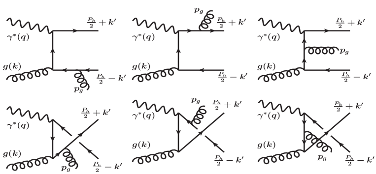
Figure 1: Feynman diagrams for $\gamma^{*}+g\rightarrow J/\psi+g$ process

The general expression of the amplitude for the bound state production of $J/\psi$ in NRQCD framework can be written as Boer and Pisano (2012); Mukherjee and Rajesh (2017a) :

$$\mathcal{M}\left(\gamma^{*}g\rightarrow Q\bar{Q}[\leftidx{{}^{2S+1}}{L}{{}_{J}}^{(1)}](P_{h})+g\right)=\sum_{L_{z}S_{z}}\int\frac{d^{3}\bm{k}^{\prime}}{(2\pi)^{3}}\Psi_{LL_{z}}(\bm{k}^{\prime})\langle LL_{z};SS_{z}|JJ_{z}\rangle$$ (15)

$$\times\mathrm{Tr}[O(q,k,P_{h},k^{\prime})\mathcal{P}_{SS_{z}}(P_{h},k^{\prime})],$$

As we have imposed a cutoff on $z$, $z<0.9$, we do not need to consider the virtual diagrams as they contribute at $z=1$. In the above equation, $2k^{\prime}$ is the relative momentum of heavy quarks and $O(q,k,P_{h},k^{\prime})$ is calculated from the Feynman diagrams. The spinors of heavy quark, anti-quark legs are absorbed into the bound state wave function. By considering contribution from all the Feynman diagrams, $O(q,k,P_{h},k^{\prime})$ is given by

$$O(q,k,P_{h},k^{\prime})=\sum_{m=1}^{6}\mathcal{C}_{m}O_{m}(q,k,P_{h},k^{\prime}).$$ (16)

Where, $O_{m},\ (m=1,2,...6)$ are corresponding to each Feynman diagrams and $\mathcal{C}_{m}$ represents the color factor of corresponding diagram. The expressions for $O_{m}$ are given below

$$O_{1}=4g^{2}_{s}(ee_{c})\varepsilon^{\rho\ast}_{\lambda_{g}}(p_{g})\gamma_{\nu}\frac{\not{P_{h}}+2\not{k}^{\prime}-2\not{q}+M}{(P_{h}+2k^{\prime}-2q)^{2}-M^{2}}\gamma_{\mu}\frac{-\not{P_{h}}+2\not{k}^{\prime}-2\not{p}_{g}+M}{(P_{h}-2k^{\prime}+2p_{g})^{2}-M^{2}}\gamma_{\rho},$$ (17)

$$O_{2}=4g^{2}_{s}(ee_{c})\varepsilon^{\rho\ast}_{\lambda_{g}}(p_{g})\gamma_{\rho}\frac{\not{P_{h}}+2\not{k}^{\prime}+2\not{p}_{g}+M}{(P_{h}+2k^{\prime}+2p_{g})^{2}-M^{2}}\gamma_{\nu}\frac{-\not{P_{h}}+2\not{k}^{\prime}+2\not{k}+M}{(P_{h}-2k^{\prime}-2k)^{2}-M^{2}}\gamma_{\mu},$$ (18)

$$O_{3}=4g^{2}_{s}(ee_{c})\varepsilon^{\rho\ast}_{\lambda_{g}}(p_{g})\gamma_{\nu}\frac{\not{P_{h}}+2\not{k}^{\prime}-2\not{q}+M}{(P_{h}+2k^{\prime}-2q)^{2}-M^{2}}\gamma_{\rho}\frac{-\not{P_{h}}+2\not{k}^{\prime}+2\not{k}+M}{(P_{h}-2k^{\prime}-2k)^{2}-M^{2}}\gamma_{\mu},$$ (19)

Here, the mass of bound state $M$ is assumed to be twice the mass of charm quark ($m_{c}$) $i.e.\ M=2m_{c}$, .The charge conjugation invariance allow us to write the expressions for ($O_{4},O_{5}$ and $O_{6}$), from the other Feynman diagrams, by reversing the fermion line and replacing $k^{\prime}$ by $-k^{\prime}$. Assuming the $Q\bar{Q}$ is formed in color singlet state, the color factor of each diagram is given by

$$\mathcal{C}_{1}=\mathcal{C}_{5}=\mathcal{C}_{6}=\sum_{ij}\langle 3i;\bar{3}j|1\rangle(t_{a}t_{b})_{ij},~{}~{}~{}\mathcal{C}_{2}=\mathcal{C}_{3}=\mathcal{C}_{4}=\sum_{ij}\langle 3i;\bar{3}j|1\rangle(t_{b}t_{a})_{ij}$$ (20)

The SU(3) Clebsch-Gordan coefficients for CS are given by

$$\langle 3i;\bar{3}j|1\rangle=\frac{\delta^{ij}}{\sqrt{N_{c}}}$$ (21)

where $N_{c}$ is the number of colors. The generators of the SU(3) group satisfies the relations: $\mathrm{Tr}(t_{a})=0,$ $\mathrm{Tr}(t_{a}t_{b})=\delta_{ab}/2$ and $\mathrm{Tr}(t_{a}t_{b}t_{c})=\frac{1}{4}(d_{abc}+if_{abc})$.

From these relations, we get the color factor for the production of $Q\bar{Q}$ pair in CS state as follows;

$$\mathcal{C}_{1}=\mathcal{C}_{2}=\mathcal{C}_{3}=\mathcal{C}_{4}=\mathcal{C}_{5}=\mathcal{C}_{6}=\frac{\delta_{ab}}{2\sqrt{N_{c}}}.$$ (22)

The spin projection operator, given in the equation of amplitude of the bound state, includes the spinors of heavy quark and anti-quark and is given by Boer and Pisano (2012):

$$\mathcal{P}_{SS_{z}}(P_{h},k^{\prime}) = \sum_{s_{1}s_{2}}\langle\frac{1}{2}s_{1};\frac{1}{2}s_{2}|SS_{z}\rangle v(\frac{P_{h}}{2}-k^{\prime},s_{1})\bar{u}(\frac{P_{h}}{2}+k^{\prime},s_{2})$$ (23)

$$= \frac{1}{4M^{3/2}}(-\not{P}_{h}+2\not{k}^{\prime}+M)\Pi_{SS_{z}}(\not{P}_{h}+2\not{k}^{\prime}+M)+\mathcal{O}(k^{\prime 2})$$

where $\Pi_{SS_{z}}=\gamma^{5}$ for singlet ($S=0$) state and $\Pi_{SS_{z}}=\not{\varepsilon}_{s_{z}}(P_{h})$ for triplet ($S=1$) state. $\varepsilon_{s_{z}}(P_{h})$ is the spin polarization vector of $Q\bar{Q}$ pair. Since, $k^{\prime}<<P_{h}$, one can perform Taylor expansion of the amplitude around $k^{\prime}=0$. In that expansion, the first term gives the S-waves(L=0,J=0,1). For the P-waves(l=1,J=0,1,2), we need to consider the linear terms in $k^{\prime}$ in the expansion as the radial wavefunction $R_{1}(0)=0$ for $P-$wave. Since, $J/\psi$ is a ${}^{3}S_{1}$ state, in the color singlet model we calculate contribution of the CS state ${}^{3}S_{1}$.

$$\mathcal{M}[\leftidx{{}^{2S+1}}{S}{{}_{J}}^{(1)}](P_{h},k) = \frac{1}{\sqrt{4\pi}}R_{0}(0)\mathrm{Tr}[O(q,k,P_{h},k^{\prime})\mathcal{P}_{SS_{z}}(P_{h},k^{\prime})]\Big{\rvert}_{k^{\prime}=0}$$ (24)

$$= \frac{1}{\sqrt{4\pi}}R_{0}(0)\mathrm{Tr}[O(0)\mathcal{P}_{SS_{z}}(0)],$$

where,

$$O(0)=O(q,k,P_{h},k^{\prime})\Big{\rvert}_{k^{\prime}=0}~{},~{}~{}~{}~{}~{}~{}~{}~{}\mathcal{P}_{SS_{z}}(0)=\mathcal{P}_{SS_{z}}(P_{h},k^{\prime})\Big{\rvert}_{k^{\prime}=0}$$ (25)

We have the following symmetry relations for ${{}^{3}}{S}{{}_{1}}$ state

$$\mathrm{Tr}[O_{1}(0)(-\not{P}_{h}+M)\not{\varepsilon}_{s_{z}}] = \mathrm{Tr}[O_{4}(0)(-\not{P}_{h}+M)\not{\varepsilon}_{s_{z}}]$$

$$\mathrm{Tr}[O_{2}(0)(-\not{P}_{h}+M)\not{\varepsilon}_{s_{z}}] = \mathrm{Tr}[O_{5}(0)(-\not{P}_{h}+M)\not{\varepsilon}_{s_{z}}]$$

$$\mathrm{Tr}[O_{3}(0)(-\not{P}_{h}+M)\not{\varepsilon}_{s_{z}}] = \mathrm{Tr}[O_{6}(0)(-\not{P}_{h}+M)\not{\varepsilon}_{s_{z}}]$$

The final expression for the amplitude for ${{}^{3}}{S}{{}_{1}}$ state is given by

$$\begin{aligned} \mathcal{M}[\leftidx{{}^{3}}{S}{{}_{1}}^{(1)}](P_{h},k)=&{}\frac{1}{4\sqrt{\pi M}}R_{0}(0)\frac{\delta_{ab}}{\sqrt{N_{c}}}\mathrm{Tr}\left[\sum_{m=1}^{3}O_{m}(0)(-\not{P}_{h}+M)\not{\varepsilon}_{s_{z}}\right],\end{aligned}$$ (27)

where

$$\begin{aligned} \sum_{m=1}^{3}O_{m}(0)=&{}g^{2}_{s}(ee_{c})\varepsilon^{\rho\ast}_{\lambda_{g}}(p_{g})\Bigg{[}\frac{\gamma_{\nu}(\not{P_{h}}-2\not{q}+M)\gamma_{\mu}(-\not{P_{h}}-2\not{p}_{g}+M)\gamma_{\rho}}{(\hat{s}-M^{2})(\hat{u}-M^{2}+q^{2})}\\ &\qquad\qquad+\frac{\gamma_{\rho}(\not{P_{h}}+2\not{p}_{g}+M)\gamma_{\nu}(-\not{P_{h}}+2\not{k}+M)\gamma_{\mu}}{(\hat{s}-M^{2})(\hat{t}-M^{2})}\\ &\qquad\qquad+\frac{\gamma_{\nu}(\not{P_{h}}-2\not{q}+M)\gamma_{\rho}(-\not{P_{h}}+2\not{k}+M)\gamma_{\mu}}{(\hat{t}-M^{2})(\hat{u}-M^{2}+q^{2})}\Bigg{]}.\end{aligned}$$

Calculation of the asymmetry

We use a framework based on generalized parton model, with the inclusion of intrinsic transverse momentum effects. We assume TMD factorization for the process considered. We consider a kinematical region in which the transverse momentum of $J/\psi$ is small compared to the mass of $J/\psi$, $M$ $i.e.~{}~{}P_{h\perp}<M$. The final gluon carries the momenta fraction $(1-z)$, as $z=\frac{P\cdot P_{h}}{P\cdot q}$, is the energy fraction transferred from the photon to $J/\psi$ in the proton rest frame. So, this means that when $~{}~{}z\rightarrow 1$, the outgoing gluon is soft. We consider $z<0.9$ to keep the final gluon hard. Moreover, gluon and heavy quark fragmentation can also contribute to quarkonium production significantly for $P_{h\perp}>4~{}GeV$. We have imposed an upper limit on $P_{h\perp}$. In order to eliminate the fragmentation of the hard gluon into $J/\psi$ we also use a lower bound on $z$, namely $0.3<z$.

In the differential cross section given in Eq. (12), there is a contraction of four tensors which is written as

$$L^{\mu\mu^{\prime}}(l,q)\Phi^{\nu\nu^{\prime}}(x,{\bm{k}}_{\perp})\mathcal{M}^{\gamma^{*}+g\rightarrow J/\psi+g}_{\mu\nu}\mathcal{M}^{*\gamma^{*}+g\rightarrow J/\psi+g}_{\mu^{\prime}\nu^{\prime}}$$ (28)

where the individual components are defined above. The summation over the transverse polarization of the final on-shell gluon is given by

$$\sum_{\lambda_{a}=1}^{2}\varepsilon^{\lambda_{a}}_{\mu}(p_{g})\varepsilon^{\ast\lambda_{a}}_{\mu^{\prime}}(p_{g})=-g_{\mu\mu^{\prime}}+\frac{p_{g\mu}n_{g\mu^{\prime}}+p_{g\mu^{\prime}}n_{g\mu}}{p_{g}\cdot n_{g}}-\frac{p_{g\mu}p_{g\mu^{\prime}}}{(p_{g}\cdot n_{g})^{2}}$$ (29)

with $n_{g}^{\mu}=\frac{P^{\mu}_{h}}{M}$. We have three amplitudes and their corresponding conjugates, given by Eq. (27), that will contribute. We use the notation

$$\begin{aligned} \mathcal{M}_{i}[\leftidx{{}^{3}}{S}{{}_{1}}^{(1)}](P_{h},k)=&{}\frac{1}{4\sqrt{\pi M}}R_{0}(0)\frac{\delta_{ab}}{\sqrt{N_{c}}}\mathrm{Tr}\left[O_{i}(0)(-\not{P}_{h}+M)\not{\varepsilon}_{s_{z}}\right],\end{aligned}$$ (30)

where $i=1,2,3$, corresponds to the contribution from each independent diagram.
So, the cross section will get contribution from nine terms $(\mathrm{of~{}the~{}form}~{}M_{i}M_{j}~{},~{}\mathrm{where}~{}i,j=1,2,3)$

$$M_{i}M_{j}=L^{\mu\mu^{\prime}}(l,q)\Phi^{\nu\nu^{\prime}}(x,{\bm{k}}_{\perp})\mathcal{M}^{\gamma^{*}+g\rightarrow J/\psi+g}_{i\mu\nu}\mathcal{M}^{*\gamma^{*}+g\rightarrow J/\psi+g}_{j\mu^{\prime}\nu^{\prime}}$$ (31)

and hence, the differential cross section can be written as

$$\begin{aligned} d\sigma=&\frac{1}{2s}\frac{d^{3}l^{\prime}}{(2\pi)^{3}2E_{l^{\prime}}}\frac{d^{3}P_{h}}{(2\pi)^{3}2E_{P_{h}}}\int\frac{d^{3}p_{g}}{(2\pi)^{3}2E_{g}}\int dxd^{2}{\bm{k}}_{\perp}(2\pi)^{4}\delta(q+k-P_{h}-p_{g})\\ &\times\frac{1}{Q^{4}}{\mid M\mid}^{2};\end{aligned}$$ (32)

where $M=\sum_{i}M_{i}$. Out of the nine terms in ${\mid M\mid}^{2}$, six are interference terms with a symmetry $M_{i}M_{j}=M_{j}M_{i}~{}~{}for~{}~{}i\neq j$. So, effectively we need to compute six terms.

In a frame where the virtual photon and target proton move along the $z$-axis, and the lepton scattering plane defines the azimuthal angles $\phi_{l}=\phi_{l^{\prime}}=0$, then we have

$$\frac{d^{3}l^{\prime}}{(2\pi)^{3}2E_{l^{\prime}}}=\frac{1}{16\pi^{2}}sydx_{B}dy,~{}~{}~{}~{}\frac{d^{3}P_{h}}{(2\pi)^{3}2E_{h}}=\frac{1}{(2\pi)^{3}}\frac{1}{2z}dzd^{2}\textbf{P}_{h\perp}$$

$$\frac{d^{3}p_{g}}{(2\pi)^{3}2E_{g}}=\frac{1}{(2\pi)^{3}}\frac{1}{2z_{2}}dz_{2}d^{2}\textbf{p}_{g\perp}$$ (33)

and the delta function can be expressed as

$$\begin{split}\delta^{4}(q+k-P_{h}-p_{g})=&\delta\Big{(}x-\frac{1}{ys}(x_{B}ys+\frac{M^{2}+P_{h\perp}^{2}}{z}+\frac{(k_{\perp}-P_{h\perp})^{2}}{(1-z)})\Big{)}\\ &\times\frac{2}{ys}\delta(1-z-z_{2})\times\delta^{2}(\textbf{k}_{\perp}-\textbf{P}_{h\perp}-\textbf{p}_{g\perp})\end{split}$$ (34)

where, the delta function sets $z_{2}=(1-z)$. Hence, after integrating with respect to $x$, $z_{2}$ and $p_{g\perp}$, the final form of the differential cross section can be given by

$$\frac{d\sigma}{dydx_{B}dzd^{2}\textbf{P}_{h\perp}}=\frac{1}{256\pi^{4}}\frac{1}{x_{B}^{2}s^{3}y^{2}z(1-z)}\int k_{\perp}dk_{\perp}{\mid M^{\prime}\mid}^{2}$$ (35)

where, ${\mid M^{\prime}\mid}^{2}=\int d\phi{\mid M\mid}^{2}$, and $k_{\perp}$ is the magnitude of ${\bf k_{\perp}}$. As we are interested in the small $x$ region, we neglect terms containing higher powers of $x_{B}$; also as $z<1$, we neglect terms containing higher powers of $z$ and kept up to $z^{2}$. We also keep terms only up to $({k^{2}_{\perp}\over M^{2}_{p}})$. The leading terms in the numerator of the $cos(2\phi_{h})$ asymmetry come only from the first Feynman diagram. These terms are given in the appendix. The denominator of the $cos(2\phi_{h})$ asymmetry, which is defined below, is simply the cross section integrated over the azimuthal angle $\phi_{h}$. The leading terms in the cross section comes from $f_{1}^{g}$ term. All the terms corresponding to $h_{1}^{\perp g}$ are suppressed by $k_{\perp}^{2}/M_{p}^{2}$. Hence, from the approximations we mentioned above, the leading terms in the cross section in the denominator of $cos(2\phi_{h})$ asymmetry are coming from $M_{1}M_{1},~{}M_{1}M_{2},~{}M_{1}M_{3}$. These contributions are given in the appendix.

The differential cross section then can be given as

$$\frac{d\sigma}{dydx_{B}dzd^{2}\textbf{P}_{hT}} =\frac{1}{256\pi^{4}}\frac{1}{x_{B}^{2}s^{3}y^{2}z(1-z)}\int k_{\perp}dk_{\perp}$$

$$\{(A_{0}+A_{1}cos\phi_{h})f_{1}^{g}(x,\textbf{k}_{\perp}^{2})\}+\frac{k_{\perp}^{2}}{M_{p}^{2}}\{(B_{0}+B_{1}cos\phi_{h}+B_{2}cos2\phi_{h})h_{1}^{\perp g}(x,\textbf{k}_{\perp}^{2})\}$$ (36)

The coefficients $A_{0},A_{1},B_{0},B_{1}$ and $B_{2}$ are given in the appendix. The $cos(2\phi)$ asymmetry is defined as

$$\langle cos(2\phi_{h})\rangle=\frac{\int d\phi_{h}cos(2\phi_{h})d\sigma}{\int d\phi_{h}d\sigma}$$ (37)

In order to estimate the $cos(2\phi_{h})$ asymmetry, we need to parametrize the TMDs. We discuss two parametrization models, Gaussian parameterization of the TMDs and McLerran-Venugopalan(MV) model. We also calculate the upper bound of the asymmetry.

II.1 Gaussian parametrization of the TMDs

Both for the linearly polarized gluon distribution and the unpolarized gluon TMD, a Gaussian parametrization is used widely in the literature. The linearly polarized gluon distribution satisfies the model independent positivity bound Mulders and Rodrigues (2001);

$$\frac{\textbf{k}_{\perp}^{2}}{2M_{p}^{2}}\left|h_{1}^{\perp g}(x,\textbf{k}_{\perp}^{2})\right|\leq f_{1}^{g}(x,\textbf{k}_{\perp}^{2})$$ (38)

The Gaussian parametrizations satisfy the positivity bound but does not saturate it. They are as follows Boer and Pisano (2012); Mukherjee and Rajesh (2016); Mukherjee and Rajesh (2017b);

$$f_{1}^{g}(x,\textbf{k}_{\perp}^{2})=f_{1}^{g}(x,\mu)\frac{1}{\pi\langle k_{\perp}^{2}\rangle}e^{-k_{\perp}^{2}/\langle k_{\perp}^{2}\rangle}$$ (39)

$$h_{1}^{\perp g}(x,\textbf{k}_{\perp}^{2})=\frac{M_{p}^{2}f_{1}^{g}(x,\mu)}{\pi\langle k_{\perp}^{2}\rangle^{2}}\frac{2(1-r)}{r}e^{1-\frac{k_{\perp}^{2}}{r\langle k_{\perp}^{2}\rangle}}$$ (40)

where, $r(0<r<1)$ is a parameter, in our numerical estimates we took $r=1/3$. $f_{1}^{g}(x,\mu)$ is the gluon collinear PDF, which is measured at the scale $\mu=\sqrt{M^{2}+P_{h\perp}^{2}}$ and it obeys the Dokshitzer-Gribov-Lipatov-Altarelli-Parisi (DGLAP) scale evolution. The width of the Gaussian, $\langle k_{\perp}^{2}\rangle$, depends on the energy scale of the process. Following Boer and Pisano (2012), we took $\langle k_{\perp}^{2}\rangle=0.25~{}\mathrm{GeV}^{2}$. The asymmetry increases on increasing model parameter $r$, reaches a maximum at $r\approx 0.4$ and then decreases, but the variation of asymmetry is very small.

II.2 Upper bound of the asymmetry

The asymmetry reaches its maximum value when the positivity bound given by Eq. (38) is saturated. Using this, we calculate the upper bound of $|\langle cos(2\phi_{h})\rangle|$ as below Pisano et al. (2013);

$$|\langle cos(2\phi_{h})\rangle| =\left|\frac{\int d\phi_{h}cos(2\phi_{h})d\sigma}{\int d\phi_{h}d\sigma}\right|$$

$$=\frac{\int k_{\perp}dk_{\perp}\textbf{k}_{\perp}^{2}|h_{1}^{\perp g}(x,\textbf{k}_{\perp}^{2})|}{\int k_{\perp}dk_{\perp}2M_{p}f_{1}^{g}(x,\textbf{k}_{\perp}^{2})}\frac{|B_{2}|}{A_{0}}\leq\frac{|B_{2}|}{A_{0}}\equiv R$$ (41)

(a)   (b)

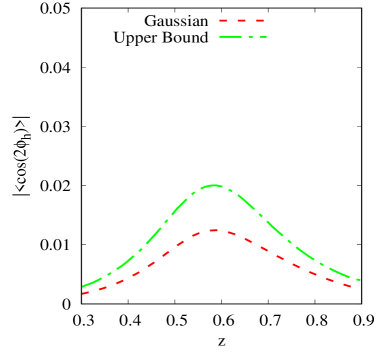
Figure 2: $cos(2\phi_{h})$ asymmetry in $e+p\rightarrow e+J/\psi+X$ process as function of (a) $P_{hT}$ (left panel) and (b) $z$ (right panel) at $\sqrt{s}=45$ GeV (EIC) and $x_{B}=0.01$. The integration ranges are $0<P_{hT}\leq 3$ GeV, $0.3<z<0.9$ and $0.05<y<0.4$. For convention of lines see the legend in the plots.

II.3 McLerran-Venugopalan (MV) model

In the small $x$ region, the Weizsäcker-Williams (WW) type gluon distribution can be calculated in MV model McLerran and Venugopalan (1994a, b, c): Within the nonperturbative McLerran-Venugopalan model, we can define the gluon distribution function inside an unpolarized large nucleus or inside an energetic proton, in the small $x$ limit. In this model, the analytical expression of the WW type unpolarized and linearly polarized gluon distributions are given by

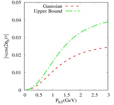
(a)   (b)

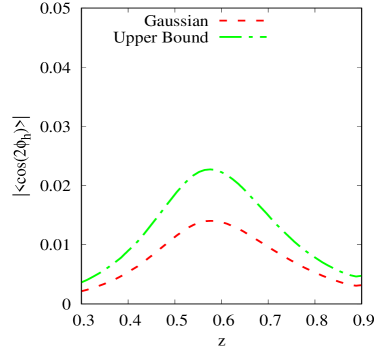
Figure 3: $cos(2\phi_{h})$ asymmetry in $e+p\rightarrow e+J/\psi+X$ process as function of (a) $P_{hT}$ (left panel) and (b) $z$ (right panel) at $\sqrt{s}=150$ GeV (EIC) and $x_{B}=0.01$. The integration ranges are $0<P_{hT}\leq 3$ GeV, $0.3<z<0.9$ and $0.005<y<0.04$. For convention of lines see the legend in the plots.

$$f_{1}^{g}(x,\textbf{k}_{\perp}^{2})=\frac{S_{\perp}C_{F}}{\alpha_{s}\pi^{3}}\int dr\frac{J_{0}(k_{\perp}r)}{r}\left(1-e^{-\frac{r^{2}}{4}Q^{2}_{sg}(r)}\right)$$ (42)

$$h_{1}^{\perp g}(x,\textbf{k}_{\perp}^{2})=\frac{S_{\perp}C_{F}}{\alpha_{s}\pi^{3}}\frac{2M_{p}^{2}}{k_{\perp}^{2}}\int dr\frac{J_{2}(k_{\perp}r)}{r\log(\frac{1}{r^{2}\Lambda_{QCD}^{2}})}\left(1-e^{-\frac{r^{2}}{4}Q^{2}_{sg}(r)}\right)$$ (43)

where $S_{\perp}$ is transverse size of the nucleus or nucleon. $Q_{sg}$ is the saturation scale, which in MV model, is defined as $Q_{sg}^{2}=\alpha_{s}N_{c}\mu_{A}\ln\frac{1}{r^{2}\Lambda_{QCD}^{2}}$ and $\mu_{A}S_{\perp}=\alpha_{s}2\pi A$, where $A=1$ for the proton. Following the approach of Bacchetta et al. (2018), we have used a regularized version of the MV model in our calculation of the asymmetry. The ratio of linearly polarized and unpolarized distribution in MV model can be given by

$$\frac{\textbf{k}_{\perp}^{2}}{2M_{p}^{2}}\frac{h_{1}^{\perp g}(x,\textbf{k}_{\perp}^{2})}{f_{1}^{g}(x,\textbf{k}_{\perp}^{2})}=\frac{\int dr\frac{J_{2}(k_{\perp}r)}{r\log(\frac{1}{r^{2}\Lambda_{QCD}^{2}})}\left(1-e^{-\frac{r^{2}}{4}Q^{2}_{sg0}\log(\frac{1}{r^{2}\Lambda_{QCD}^{2}})}\right)}{\int dr\frac{J_{0}(k_{\perp}r)}{r}\left(1-e^{-\frac{r^{2}}{4}Q^{2}_{sg0}\log(\frac{1}{r^{2}\Lambda_{QCD}^{2}})}\right)}$$ (44)

For $Q^{2}_{sg0}=(N_{c}/C_{F})\times Q^{2}_{s0}$, where $Q^{2}_{s0}=0.35~{}{\mathrm{GeV}}^{2}$ at $x=0.01$ and $\Lambda_{QCD}=0.2~{}{\mathrm{GeV}}$, the ratio is below $1$ for all $k_{\perp}$. Below we give our numerical results.

III Numerical Results

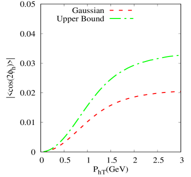
(a)   (b)

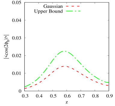
Figure 4: $cos(2\phi_{h})$ asymmetry in $e+p\rightarrow e+J/\psi+X$ process as function of (a) $P_{hT}$ (left panel) and (b) $z$ (right panel) at $\sqrt{s}=190$ GeV (EIC) and $x_{B}=0.005$. The integration ranges are $0<P_{hT}\leq 3$ GeV, $0.3<z<0.9$ and $0.006<y<0.05$. For convention of lines see the legend in the plots.

We have estimated the $cos(2\phi_{h})$ asymmetry in $J/\psi$ production in the kinematics of EIC. MSTW2008 Martin et al. (2009) is used for collinear PDFs. We have used the DGLAP evolution for the collinear pdfs. We have not included TMD evolution. As stated in the introduction, we have used cuts on $z$, $0.3<z<0.9$. As we know, gluon initiated processes are enhanced at small $x$. In fact, small $x$ values will be accessed at EIC, and this kinematical region will be very important in determining the gluon TMDs including the linearly polarized gluon TMD. In this work, we have studied the $cos~{}2\phi$ asymmetry for EIC in the small $x$ region. It is to be noted that $x$ is related to the Bjorken variable $x_{B}$ through Eq. 9. Smaller $x$ values also restrict $Q^{2}$ to be small, in this work we took $Q^{2}$ to be of the same order and bounded by $M^{2}$ ($1<Q^{2}<9~{}\mathrm{GeV}^{2}$) , which is the mass of $J/\psi$. For both the parametrizations used, the asymmetry is negative, which is consistent with the LO calculation Mukherjee and Rajesh (2017a). In the plots, we show the magnitude of the asymmetry. CS LDMEs can be found for example in Chao et al. (2012). As only one state contributes in the CS model, namely ${{}^{3}}{S}{{}_{1}}$ the asymmetry does not depend on the specific set of LDME. This is different from the CO model, where even at LO, contribution comes from several states Mukherjee and Rajesh (2017a), and the result depends on the choice of LDMEs. However, the unpolarized cross section will depend on the choice of LDMEs in both the models. In our previous work Mukherjee and Rajesh (2017a), we compared with three set of LDMEs where one sets of LDMEs giving the unpolarized cross section that matches more with the experimental data than the other sets. Figs. 2 , 3 and 4 show the upper bound of the asymmetry as well as an estimate using the Gaussian model, at $\sqrt{s}=45$ GeV, $150$ GeV and $190$ GeV respectively, as a function of $P_{hT}$ and $z$ . Corresponding $x_{B}$ values are $x_{B}=0.01,~{}0.01$ and $0.005$ respectively; ranges of $y$ integration are $0.05<y<0.4,~{}0.005<y<0.04$ and $0.006<y<0.05$ respectively. $y$ is constrained by the choice of $Q^{2}$ and $x_{B}$. The transverse momentum $P_{h\perp}$ of $J/\psi$ is taken in range $0<P_{h\perp}<3$  GeV. Energy fraction $z$ is in the range $0.3<z<0.9$ for all these plots. The upper bound of the asymmetry increases with increase of $\sqrt{s}$ for the same $x_{B}$, it reaches maximum near $P_{hT}\approx 3$  GeV, the maximum is about $4\%$ for $\sqrt{s}=150$ GeV. However, for smaller $x_{B}$, asymmetry decreases. The asymmetry reaches a peak near $z=0.6$ for the kinematical cuts chosen. The qualitative behavior of the asymmetry remains the same for all $\sqrt{s}$. The Gaussian model gives smaller asymmetry. Fig. 5 shows a comparison of the upper bound of the asymmetry with that calculated in Gaussian model as well as MV model, as a function of $P_{hT}$, for two different values of $z$, (a) $z=0.5$ and (b) $z=0.7$. For both these plots we have taken fixed value of $x=0.01$, $Q^{2}=9~{}{\mathrm{GeV}}^{2}$ and $0.2<y<1$. For (a) $\sqrt{s}$ is in the range $61$ to $181$  GeV, and for (b) $\sqrt{s}$ is in the range $58$ to $182$  GeV. Asymmetry in the MV model is smaller compared to the Gaussian model, and both lie below the upper bound. The asymmetry is higher for higher values of $z$.

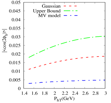
(a)   (b)

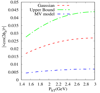
Figure 5: $cos(2\phi_{h})$ asymmetry in $e+p\rightarrow e+J/\psi+X$ process as function of $P_{hT}$ for (a) fixed $Q^{2}=9~{}{\mathrm{GeV}}^{2}$, $x=0.01$ and $z=0.5$ and (b) fixed $Q^{2}=9~{}{\mathrm{GeV}}^{2}$, $x=0.01$ and $z=0.7$. In both the case integration range on $y$ is $0.2<y<1$. For convention of lines see the legend in the plots.

IV conclusion

In this work, we have calculated the $cos~{}2\phi$ asymmetry in electroproduction of $J/\psi$ at EIC, that probes the linearly polarized gluon distribution in the unpolarized proton. We calculated the asymmetry in the kinematical region $z<1$, where the NLO subprocess $\gamma^{*}+g\rightarrow J/\psi+g$ gives the leading contribution. The gluon TMDs probed in this process are of Weizsäcker-Williams (WW) type. As gluon distributions pay an important role in the small $x$ region, we investigate the asymmetry in the small $x$ kinematical region, using a Gaussian parametrization of the TMDs as well as in McLerran-Venugopalan model. We also show the upper bound of the asymmetry saturating the inequality for the linearly polarized gluon distribution. At EIC, low values of $x$ also restrict the $Q^{2}$ (virtuality of the photon) values. We have calculated the $J/\psi$ production amplitude in NRQCD based color singlet (CS) approach. The asymmetry in the kinematical region considered is small but sizable. The magnitude of the asymmetry may depend on the production mechanism of the quarkonium. As shown in Mukherjee and Rajesh (2017a), CS mechanism underestimates the $J/\psi$ production at HERA, and both CS and CO contributions are needed to describe the data. In CO formalism contribution will come from several LDMEs in the final state, which may enhance the asymmetry. We plan to see the effect of the CO mechanism on the asymmetry in a future work. Another interesting study would be the effect of small-$x$ evolution on the asymmetry. In any case, the $cos~{}2\phi$ asymmetry in $J/\psi$ production at the EIC will be an important tool to gain information on the WW type linearly polarized gluon distribution.

V Acknowledgement

We thank P. J. Mulders, E. Petreska and D. Boer for discussion. Part of the work of AM was done at NIKHEF, Amsterdam, the visit was supported by the European Research Council under the ”Ideas” program QWORK (contract 320389).

VI Appendix

All the amplitude squares and the coefficients are integrated over $\phi$, where $\phi$ and $\phi_{h}$ are the azimuthal angle of initial gluon and $J/\psi$ respectively.

$$M^{\prime}_{i}M^{\prime}_{j}=\int d\phi M_{i}M_{j}$$ (45)

$$\begin{split}M^{\prime}_{1}M^{\prime}_{1}=&\big{\{}f_{1}^{g}\times 128\pi M^{4}\big{\{}M^{4}(z-1)^{3}+M^{2}\big{(}{P_{h\perp}}^{2}(z-1)(8(z-1)z+3)\\ &+sy\big{(}{x_{B}}\big{(}z\big{(}(1-6y(y+2))z^{2}\\ &+2y(y+4)z-2y+z+1\big{)}-1\big{)}-x(z-1)^{3}\big{)}\big{)}\\ &+2{P_{h\perp}}\sqrt{{x_{B}}}\sqrt{1-y}z\sqrt{sy}\cos({\phi_{h}})\big{(}M^{2}(z(4z-5)+2)\\ &+{P_{h\perp}}^{2}(z(24z-17)+4)-2sxy(z(4z-3)+1)\big{)}\\ &+{P_{h\perp}}^{4}(z(z(11z-23)+13)-3)+{P_{h\perp}}^{2}sy\big{(}x(z(-2(z-5)z-9)+3)\\ &+{x_{B}}\left(z\left(-3(y(5y+16)-6)z^{2}+2(y(y+14)-5)z-6y+7\right)-3\right)\big{)}\\ &+s^{2}x{x_{B}}y^{2}z(z((y-2)y(2z-1)+2(8z-7))+4)\big{\}}\\ &+\frac{k_{\perp}^{2}h_{1}^{\perp g}}{M_{p}^{2}}\times 64\pi M^{4}\big{\{}M^{4}\left(-(z-1)^{3}\right)+M^{2}\big{(}{P_{h\perp}}^{2}(z(-4(z-2)z-7)+3)\\ &+sy\big{(}x(z-1)^{3}+{x_{B}}z\big{(}(y(7y+18)-7)z^{2}-2y(2y+5)z\\ &+2y+z-1\big{)}+{x_{B}}\big{)}\big{)}+2{P_{h\perp}}\sqrt{{x_{B}}}z\big{(}{P_{h\perp}}s\sqrt{{x_{B}}}(y-1)y(z(5z-4)+2)\\ &\times\cos(2\phi_{h})-\sqrt{1-y}\sqrt{sy}\cos(\phi_{h})\big{(}M^{2}(1-3z)^{2}+{P_{h\perp}}^{2}(z(13z-12)+5)\\ &+sxy(z(6z-5)+2)\big{)}\big{)}+{P_{h\perp}}^{4}(z((7-3z)z-6)+3)\\ &+{P_{h\perp}}^{2}sy\big{(}{x_{B}}\big{(}z\big{(}(3y(3y+8)-22)z^{2}-2(y(y+13)-8)z\\ &+10y-9\big{)}+3\big{)}-x(z(2z(z+1)-5)+3)\big{)}\\ &-s^{2}xy^{2}z\big{(}x\left(6z^{2}-4z+1\right)+{x_{B}}z\big{(}(y-2)y(4z-3)\\ &+26z-20\big{)}-2{x_{B}}(y-3)\big{)}\big{\}}\big{\}}/\big{\{}xy^{2}(z-1)^{2}z\left(M^{2}+sy({x_{B}}-x)\right)^{2}\\ &\times\left(M^{2}+{P_{h\perp}}^{2}-s{x_{B}}y(z-2)z\right)^{2}\big{\}}\\ \end{split}$$ (46)

$$\begin{split}M^{\prime}_{1}M^{\prime}_{2}=&\big{\{}f_{1}^{g}\times 64\pi M^{6}\big{\{}M^{2}(z-1)(2z-3)+{P_{h\perp}}^{2}(2z(4z-9)+9)\\ &-2{P_{h\perp}}\sqrt{{x_{B}}}\sqrt{1-y}(z-1)z(3z-8)\sqrt{sy}\cos({\phi_{h}})\\ &-sy(z-1)\big{(}x(z+1)(2z-3)+{x_{B}}z\big{(}3(y(y+6)-6)z^{2}\\ &-6(y(y+4)-3)z+4y+3\big{)}+2{x_{B}}y+{x_{B}}\big{)}\big{\}}\\ &-\frac{k_{\perp}^{2}h_{1}^{\perp g}}{M_{p}^{2}}\times 32\pi M^{6}\big{\{}M^{2}(z-1)(2z-3)+{P_{h\perp}}^{2}(2z(3z-7)+7)\\ &-2{P_{h\perp}}\sqrt{{x_{B}}}\sqrt{1-y}(z-1)(2z-3)(3z+1)\sqrt{sy}\cos({\phi_{h}})\\ &-sy(z-1)\big{(}x(3z-5)+{x_{B}}z\big{(}(y(5y+6)-6)z^{2}-2y(5y+7)z\\ &+2y(y+2)+6z+5\big{)}+{x_{B}}(4y-1)\big{)}\big{\}}\big{\}}/\big{\{}sx^{2}y^{3}(z-1)z^{3}\\ &\times\left(M^{2}+sy({x_{B}}-x)\right)^{2}\left(M^{2}+{P_{h\perp}}^{2}-s{x_{B}}y(z-2)z\right)\big{\}}\end{split}$$ (47)

$$\begin{split}M^{\prime}_{1}M^{\prime}_{3}=&\big{\{}-f_{1}^{g}\times 64\pi M^{8}\big{\{}2M^{2}(z-1)^{2}(3z-5)+4{P_{h\perp}}^{2}(z-1)(z(6z-13)+8)\\ &-2{P_{h\perp}}\sqrt{{x_{B}}}\sqrt{1-y}(z-1)^{2}(z(14z-25)+2)\sqrt{sy}\cos({\phi_{h}})\\ &+sy\big{(}-x(3z-10)(z-1)^{2}+{x_{B}}z\big{(}y^{2}(z(z(31z-57)+43)-9)\\ &+2y(z(z(31z-59)+53)-23)-2z(5z(5z-8)+39)+56\big{)}\\ &-2{x_{B}}((y-4)y+10)\big{)}\big{\}}\\ &+\frac{k_{\perp}^{2}h_{1}^{\perp g}}{M_{p}^{2}}\times 32\pi M^{8}\big{\{}2M^{2}(z-1)^{2}(7z-9)+2{P_{h\perp}}^{2}(z-1)(z(14z-41)+29)\\ &-4{P_{h\perp}}\sqrt{{x_{B}}}\sqrt{1-y}(z-1)^{2}(7z(2z-3)+3)\sqrt{sy}\cos({\phi_{h}})\\ &+sy\big{(}{x_{B}}\big{(}y^{2}(z(z(z(55z-79)+45)-3)-4)\\ &+2y(z(z(z(59z-96)+76)-30)+5)\\ &+2z(z((51-43z)z-44)+37)-30\big{)}\\ &-x(z-1)^{2}(3z(4z+1)-14)\big{)}\big{\}}\big{\}}/\big{\{}sx^{2}y^{3}(z-1)^{2}z^{2}\left(M^{2}+sy({x_{B}}-x)\right)^{2}\\ &\times\left(M^{2}+{P_{h\perp}}^{2}-s{x_{B}}y(z-2)z\right)^{2}\big{\}}\end{split}$$ (48)

and the coefficients in final expression of cross section, Eq. (Calculation of the asymmetry), are as follows:

$$\begin{split}A_{0}=&64\pi M^{4}\big{\{}\big{\{}M^{2}(z-1)\left(M^{2}+{P_{h\perp}}^{2}-s{x_{B}}y(z-2)z\right)\big{(}M^{2}(z-1)(2z-3)\\ &+{P_{h\perp}}^{2}(2z(4z-9)+9)-sy(z-1)\big{(}x(z+1)(2z-3)\\ &+{x_{B}}z\left(3(y(y+6)-6)z^{2}-6(y(y+4)-3)z+4y+3\right)+2{x_{B}}y+{x_{B}}\big{)}\big{)}\\ &+M^{4}z\big{(}-2M^{2}(z-1)^{2}(3z-5)-4{P_{h\perp}}^{2}(z-1)(z(6z-13)+8)\\ &+sy\big{(}x(3z-10)(z-1)^{2}+{x_{B}}z\big{(}(50-31y(y+2))z^{3}\\ &+(y(57y+118)-80)z^{2}-y(43y+106)z\\ &+y(9y+46)+78z-56\big{)}+2{x_{B}}((y-4)y+10)\big{)}\big{)}\big{\}}/s\\ &+2xyz^{2}\big{(}M^{4}(z-1)^{3}+M^{2}\big{(}{P_{h\perp}}^{2}(z-1)(8(z-1)z+3)\\ &+sy\big{(}{x_{B}}\left(z\left((1-6y(y+2))z^{2}+2y(y+4)z-2y+z+1\right)-1\right)\\ &-x(z-1)^{3}\big{)}\big{)}+{P_{h\perp}}^{4}(z(z(11z-23)+13)-3)\\ &+{P_{h\perp}}^{2}sy\big{(}x(z(-2(z-5)z-9)+3)+{x_{B}}\big{(}z\big{(}-3(y(5y+16)-6)z^{2}\\ &+2(y(y+14)-5)z-6y+7\big{)}-3\big{)}\big{)}\\ &+s^{2}x{x_{B}}y^{2}z(z((y-2)y(2z-1)+2(8z-7))+4)\big{)}\big{\}}/\big{\{}x^{2}y^{3}(z-1)^{2}z^{3}\\ &\times\left(M^{2}+sy({x_{B}}-x)\right)^{2}\left(M^{2}+{P_{h\perp}}^{2}-s{x_{B}}y(z-2)z\right)^{2}\big{\}}\end{split}$$ (49)

$$\begin{split}A_{1}=&-128\pi M^{4}{P_{h\perp}}\sqrt{{x_{B}}}\sqrt{1-y}\big{\{}-2M^{4}(z-1)^{2}(7(z-2)z+5)\\ &+M^{2}\big{(}{P_{h\perp}}^{2}(z-1)^{2}(3z-8)-syz\big{(}2xz(z(4z-5)+2)\\ &+{x_{B}}(z-2)(3z-8)(z-1)^{2}\big{)}\big{)}+2sxyz^{2}\big{(}{P_{h\perp}}^{2}((17-24z)z-4)\\ &+2sxy(z(4z-3)+1)\big{)}\big{\}}/\big{\{}x^{2}y^{2}(z-1)^{2}z^{2}\sqrt{sy}\left(M^{2}+sy({x_{B}}-x)\right)^{2}\\ &\times\left(M^{2}+{P_{h\perp}}^{2}-s{x_{B}}y(z-2)z\right)^{2}\big{\}}\end{split}$$ (50)

$$\begin{split}B_{0}=&32\pi M^{4}\big{\{}\big{\{}-M^{2}(z-1)\big{(}M^{2}+{P_{h\perp}}^{2}-s{x_{B}}y(z-2)z\big{)}\big{(}M^{2}(z-1)(2z-3)\\ &+{P_{h\perp}}^{2}(2z(3z-7)+7)-sy(z-1)\big{(}x(3z-5)+{x_{B}}z\big{(}(y(5y+6)-6)z^{2}\\ &-2y(5y+7)z+2y(y+2)+6z+5\big{)}+{x_{B}}(4y-1)\big{)}\big{)}\\ &+M^{4}z\big{(}2M^{2}(z-1)^{2}(7z-9)+2{P_{h\perp}}^{2}(z-1)(z(14z-41)+29)\\ &+sy\big{(}{x_{B}}\big{(}y^{2}(z(z(z(55z-79)+45)-3)-4)\\ &+2y(z(z(z(59z-96)+76)-30)+5)\\ &+2z(z((51-43z)z-44)+37)-30\big{)}\\ &-x(z-1)^{2}(3z(4z+1)-14)\big{)}\big{)}\big{\}}/{s}\\ &-2xyz^{2}\big{(}M^{4}(z-1)^{3}+M^{2}\big{(}{P_{h\perp}}^{2}(z-1)(4(z-1)z+3)\\ &-sy\big{(}x(z-1)^{3}+{x_{B}}z\big{(}(y(7y+18)-7)z^{2}\\ &-2y(2y+5)z+2y+z-1\big{)}+{x_{B}}\big{)}\big{)}\\ &+{P_{h\perp}}^{4}(z(z(3z-7)+6)-3)+{P_{h\perp}}^{2}sy\big{(}x(z(2z(z+1)-5)+3)\\ &+{x_{B}}\big{(}z\big{(}(22-3y(3y+8))z^{2}+2(y(y+13)-8)z\\ &-10y+9\big{)}-3\big{)}\big{)}+s^{2}xy^{2}z\big{(}x\big{(}6z^{2}-4z+1\big{)}\\ &+{x_{B}}z((y-2)y(4z-3)+26z-20)-2{x_{B}}(y-3)\big{)}\big{)}\big{\}}/\big{\{}x^{2}y^{3}(z-1)^{2}z^{3}\\ &\times\left(M^{2}+sy({x_{B}}-x)\right)^{2}\left(M^{2}+{P_{h\perp}}^{2}-s{x_{B}}y(z-2)z\right)^{2}\big{\}}\end{split}$$ (51)

$$\begin{split}B_{1}=&-64\pi M^{4}{P_{h\perp}}\sqrt{{x_{B}}}\sqrt{1-y}\big{\{}M^{4}(z-1)^{2}(z(4z(7z-12)+13)+3)\\ &+M^{2}\big{(}syz\left(2x(1-3z)^{2}z^{2}+{x_{B}}(z-2)(2z-3)(3z+1)(z-1)^{2}\right)\\ &-{P_{h\perp}}^{2}(z-1)^{2}(2z-3)(3z+1)\big{)}+2sxyz^{3}\big{(}{P_{h\perp}}^{2}(z(13z-12)+5)\\ &+sxy(z(6z-5)+2)\big{)}\big{\}}/\big{\{}x^{2}y^{2}(z-1)^{2}z^{3}\sqrt{sy}\left(M^{2}+sy({x_{B}}-x)\right)^{2}\\ &\times\left(M^{2}+{P_{h\perp}}^{2}-s{x_{B}}y(z-2)z\right)^{2}\big{\}}\end{split}$$ (52)

$$\begin{split}B_{2}=&\big{\{}128\pi M^{4}{P_{h\perp}}^{2}s{x_{B}}(y-1)(z(5z-4)+2)\big{\}}/\big{\{}xy(z-1)^{2}\\ &\times\left(M^{2}+sy({x_{B}}-x)\right)^{2}\left(M^{2}+{P_{h\perp}}^{2}-s{x_{B}}y(z-2)z\right)^{2}\big{\}}\end{split}$$ (53)

References

- Mulders and Rodrigues (2001) P. J. Mulders and J. Rodrigues, Phys. Rev. D63, 094021 (2001), eprint hep-ph/0009343.
- Lansberg et al. (2018) J.-P. Lansberg, C. Pisano, F. Scarpa, and M. Schlegel, Phys. Lett. B784, 217 (2018), eprint 1710.01684.
- Buffing et al. (2013) M. G. A. Buffing, A. Mukherjee, and P. J. Mulders, Phys. Rev. D88, 054027 (2013), eprint 1306.5897.
- Kovchegov and Mueller (1998) Y. V. Kovchegov and A. H. Mueller, Nucl. Phys. B529, 451 (1998), eprint hep-ph/9802440.
- McLerran and Venugopalan (1999) L. D. McLerran and R. Venugopalan, Phys. Rev. D59, 094002 (1999), eprint hep-ph/9809427.
- Dominguez et al. (2012) F. Dominguez, J.-W. Qiu, B.-W. Xiao, and F. Yuan, Phys. Rev. D85, 045003 (2012), eprint 1109.6293.
- Iancu et al. (2002) E. Iancu, A. Leonidov, and L. McLerran, in QCD perspectives on hot and dense matter. Proceedings, NATO Advanced Study Institute, Summer School, Cargese, France, August 6-18, 2001 (2002), pp. 73–145, eprint hep-ph/0202270.
- Kharzeev et al. (2003) D. Kharzeev, Y. V. Kovchegov, and K. Tuchin, Phys. Rev. D68, 094013 (2003), eprint hep-ph/0307037.
- Boer et al. (2016) D. Boer, S. Cotogno, T. van Daal, P. J. Mulders, A. Signori, and Y.-J. Zhou, JHEP 10, 013 (2016), eprint 1607.01654.
- Dominguez et al. (2011a) F. Dominguez, B.-W. Xiao, and F. Yuan, Phys. Rev. Lett. 106, 022301 (2011a), eprint 1009.2141.
- Metz and Zhou (2011) A. Metz and J. Zhou, Phys. Rev. D84, 051503 (2011), eprint 1105.1991.
- Schafer and Zhou (2013) A. Schafer and J. Zhou, Phys. Rev. D88, 014008 (2013), eprint 1302.4600.
- Akcakaya et al. (2013) E. Akcakaya, A. Schäfer, and J. Zhou, Phys. Rev. D87, 054010 (2013), eprint 1208.4965.
- Dumitru et al. (2015) A. Dumitru, T. Lappi, and V. Skokov, Phys. Rev. Lett. 115, 252301 (2015), eprint 1508.04438.
- Marquet et al. (2018) C. Marquet, C. Roiesnel, and P. Taels, Phys. Rev. D97, 014004 (2018), eprint 1710.05698.
- Dominguez et al. (2011b) F. Dominguez, C. Marquet, B.-W. Xiao, and F. Yuan, Phys. Rev. D83, 105005 (2011b), eprint 1101.0715.
- Boer et al. (2017) D. Boer, P. J. Mulders, J. Zhou, and Y.-j. Zhou, JHEP 10, 196 (2017), eprint 1702.08195.
- Meissner et al. (2007) S. Meissner, A. Metz, and K. Goeke, Phys. Rev. D76, 034002 (2007), eprint hep-ph/0703176.
- Pisano et al. (2013) C. Pisano, D. Boer, S. J. Brodsky, M. G. A. Buffing, and P. J. Mulders, JHEP 10, 024 (2013), eprint 1307.3417.
- Mukherjee and Rajesh (2017a) A. Mukherjee and S. Rajesh, Eur. Phys. J. C77, 854 (2017a), eprint 1609.05596.
- Boer et al. (2009) D. Boer, P. J. Mulders, and C. Pisano, Phys. Rev. D80, 094017 (2009), eprint 0909.4652.
- Efremov et al. (2018a) A. V. Efremov, N. Ya. Ivanov, and O. V. Teryaev, Phys. Lett. B777, 435 (2018a), eprint 1711.05221.
- Efremov et al. (2018b) A. V. Efremov, N. Y. Ivanov, and O. V. Teryaev, Phys. Lett. B780, 303 (2018b), eprint 1801.03398.
- Lansberg et al. (2017) J.-P. Lansberg, C. Pisano, and M. Schlegel, Nucl. Phys. B920, 192 (2017), eprint 1702.00305.
- Dumitru et al. (2018) A. Dumitru, V. Skokov, and T. Ullrich (2018), eprint 1809.02615.
- Sun et al. (2011) P. Sun, B.-W. Xiao, and F. Yuan, Phys. Rev. D84, 094005 (2011), eprint 1109.1354.
- Boer et al. (2013) D. Boer, W. J. den Dunnen, C. Pisano, and M. Schlegel, Phys. Rev. Lett. 111, 032002 (2013), eprint 1304.2654.
- Boer et al. (2012) D. Boer, W. J. den Dunnen, C. Pisano, M. Schlegel, and W. Vogelsang, Phys. Rev. Lett. 108, 032002 (2012), eprint 1109.1444.
- Echevarria et al. (2015) M. G. Echevarria, T. Kasemets, P. J. Mulders, and C. Pisano, JHEP 07, 158 (2015), [Erratum: JHEP05,073(2017)], eprint 1502.05354.
- Boer and Pisano (2012) D. Boer and C. Pisano, Phys. Rev. D86, 094007 (2012), eprint 1208.3642.
- Mukherjee and Rajesh (2017b) A. Mukherjee and S. Rajesh, Phys. Rev. D95, 034039 (2017b), eprint 1611.05974.
- Mukherjee and Rajesh (2016) A. Mukherjee and S. Rajesh, Phys. Rev. D93, 054018 (2016), eprint 1511.04319.
- Bodwin et al. (1995) G. T. Bodwin, E. Braaten, and G. P. Lepage, Phys. Rev. D51, 1125 (1995), [Erratum: Phys. Rev.D55,5853(1997)], eprint hep-ph/9407339.
- Lepage et al. (1992) G. P. Lepage, L. Magnea, C. Nakhleh, U. Magnea, and K. Hornbostel, Phys. Rev. D46, 4052 (1992), eprint hep-lat/9205007.
- Carlson and Suaya (1976) C. E. Carlson and R. Suaya, Phys. Rev. D14, 3115 (1976).
- Berger and Jones (1981) E. L. Berger and D. L. Jones, Phys. Rev. D23, 1521 (1981).
- Baier and Ruckl (1981) R. Baier and R. Ruckl, Phys. Lett. 102B, 364 (1981).
- Baier and Ruckl (1982) R. Baier and R. Ruckl, Nucl. Phys. B201, 1 (1982).
- Braaten and Fleming (1995) E. Braaten and S. Fleming, Phys. Rev. Lett. 74, 3327 (1995), eprint hep-ph/9411365.
- Cho and Leibovich (1996a) P. L. Cho and A. K. Leibovich, Phys. Rev. D53, 150 (1996a), eprint hep-ph/9505329.
- Cho and Leibovich (1996b) P. L. Cho and A. K. Leibovich, Phys. Rev. D53, 6203 (1996b), eprint hep-ph/9511315.
- D’Alesio et al. (2017) U. D’Alesio, F. Murgia, C. Pisano, and P. Taels, Phys. Rev. D96, 036011 (2017), eprint 1705.04169.
- Rajesh et al. (2018) S. Rajesh, R. Kishore, and A. Mukherjee, Phys. Rev. D98, 014007 (2018), eprint 1802.10359.
- McLerran and Venugopalan (1994a) L. D. McLerran and R. Venugopalan, Phys. Rev. D49, 2233 (1994a), eprint hep-ph/9309289.
- McLerran and Venugopalan (1994b) L. D. McLerran and R. Venugopalan, Phys. Rev. D49, 3352 (1994b), eprint hep-ph/9311205.
- McLerran and Venugopalan (1994c) L. D. McLerran and R. Venugopalan, Phys. Rev. D50, 2225 (1994c), eprint hep-ph/9402335.
- Bacchetta et al. (2018) A. Bacchetta, D. Boer, C. Pisano, and P. Taels (2018), eprint 1809.02056.
- Martin et al. (2009) A. D. Martin, W. J. Stirling, R. S. Thorne, and G. Watt, Eur. Phys. J. C63, 189 (2009), eprint 0901.0002.
- Chao et al. (2012) K.-T. Chao, Y.-Q. Ma, H.-S. Shao, K. Wang, and Y.-J. Zhang, Phys. Rev. Lett. 108, 242004 (2012), eprint 1201.2675.