Bulk Spectrum and $K$-theory for Infinite-Area Topological Quasicrystals

Abstract.

The bulk spectrum of a possible Chern insulator on a quasicrystalline lattice is examined. The effect of being a 2D insulator seems to override any fractal properties in the spectrum. We compute that the spectrum is either two continuous bands, or that any gaps other than the main gap are small. After making estimates on the spectrum, we deduce a finite system size, above which the $K$-theory must coincide with the $K$-theory of the infinite system. Knowledge of the spectrum and $K$-theory of the infinite-area system will control the spectrum and $K$-theory of sufficiently large finite systems.

The relation between finite volume $K$-theory and infinite volume Chern numbers is only proven to begin, for the model under investigation here, for systems on Hilbert space of dimension around 17 million. The real-space method based on the Clifford spectrum allows for computing Chern numbers for systems on Hilbert space of dimension around $2.7$ million. New techniques in numerical $K$-theory are used to equate the $K$-theory of systems of different sizes.

1. Introduction

Recent research [2, 14, 18, 34] shows that topological insulators and superconductors can occur as a quasicrystal. There is $K$-theory [12, 17, 18] associated to gaps in the bulk spectrum, and edge states [14, 17, 34] that arise within these gaps at the boundaries of finite systems. In the crystalline case, we have little doubt as to how to define and calculate the bulk spectrum, so most of the discussion has been on how to detect and calculate $K$-theory.

Let us step away from the $K$-theory for a while, and ponder: what is the bulk spectrum for the Hamiltonian in a tight-binding model on a quasicrystalline lattice, and how do we compute it?

A noncontroversial means to define bulk spectrum is simply to use the spectrum of the Hamiltonian for the system on full, infinite-area quasicrystalline lattice. The issue is how is a physicist to compute this? We have lost translation invariance, so cannot use momentum space to reduce the calculation to finding the spectrum of a parameterized collection of small matrices. Perhaps also gone is approximating the bulk spectrum by the spectrum of a finite sample with periodic boundary conditions.

One can impose periodic boundary conditions on a periodic approximation to the quasilattice, at the cost of introducing a few defects [2, 35]. It is not clear exactly the relation between the spectrum of these finite systems and that of the infinite system. Perhaps more theoretical work using more explicitly $C^{*}$-algebras, such as in [3, 4, 29], can settle this issue.

Another method to investigate the bulk spectrum of a quasiperiodic Hamiltonian is to look at the effect of self-similarity. This method was applied [32] to a Hamiltonian different from the one studied here, but also on the Ammann-Beenker tiling. This system had no topological index to confound the picture and the conclusion on the bulk spectrum was very different from what is presented here.

Wanting to know the spectrum of the infinite system is more than a fascinating mathematical question. It provides a manner to predict the behavior of finite systems of arbitrarily large size. We hope that the edge phenomena seen in specific finite systems of one or two sizes will persist in larger systems. However, we shall see that there are edge phenomena associated to apparent small gaps in “the bulk spectrum” of modest-sized systems and we can not easily tell if these gaps will disappear when we look at larger systems.

We will focus on a single infinite-area Hamiltonian because the numerical computations of the bulk spectrum are somewhat demanding. Specifically we investigate the “$p_{x}+ip_{y}$” tight-binding model on the Ammann-Beenker tiling, introduced in previous work with Fulga and Pikulin [14]. After numerically estimating the bulk spectrum, we are able to calculate a size above which all finite models have the same $K$-theory as the infinite model. We find an indirect way to calculate the $K$-theory associated to one such infinite model, thus providing solid evidence that the infinite system has Chern number $-1$.

The methods introduced do not depend on the structure of the quasilattice. They can be implemented whenever the Hamiltonian is local and bounded, although the accuracy and efficiency are expected to vary according to the structure of the quasilattice.

2. A tight-binding Hamiltonian on a Quasicrystal

We will investigate the “$p_{x}+ip_{y}$” tight-binding model on the Ammann-Beenker tiling [5]. A small system using this Hamiltonian was examined previously [14]. The Hilbert space is $\ell^{2}(\mathcal{V})\otimes\mathbb{C}^{2}$, where $\mathcal{G}=(\mathcal{E},\mathcal{V})$ is the graph whose edges and vertices are taken from the tiles of an Ammann-Beenker tiling of the plane. Define $H_{\mathrm{QC}}$, a bounded Hermitian operator on $\ell^{2}(\mathcal{V})\otimes\mathbb{C}^{2}$, as an infinite matrix with

$$H_{j}=-\mu\sigma_{z},$$

a term associated with each site (vertex), and

$$H_{jk}=-t\sigma_{z}-\frac{i}{2}\Delta\sigma_{x}\cos(\theta_{jk})-\frac{i}{2}\Delta\sigma_{y}\sin(\theta_{jk}),$$

a hopping term associated to each edge. The angle is taken from a reference angle, as illustrated in Figure 2.1.

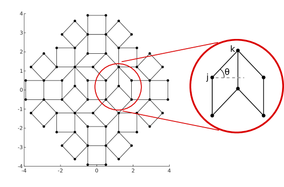
Figure 2.1. Defining the infinite-area Hamiltonian $H_{\mathrm{QC}}$, determined by the quasilattice. Shown is the definition of the angles $\theta=\theta_{jk}$ associated to the $j$-$k$ term. We define the lattice unit to be the common length of all the edges.

3. Working around Edge States

A direct approach to estimating the bulk spectrum is to put Dirichlet boundary conditions on a finite sample, compute the spectrum of the finite Hamiltonian, and sort those eigenvalues according to whether the associated eigenvector seems to be localized at the edge or not. This technique has certainly been used before [2] for this purpose. We prefer to use round samples, as theory [21] suggests that the smallest distance to the center of a sample is what dictates the strength of small system size effects. Also, this was the choice made in a earlier study [30] of an ordinary insulator on a quasilattice. A typical round portion of the quasilattice is shown in Figure 3.1.

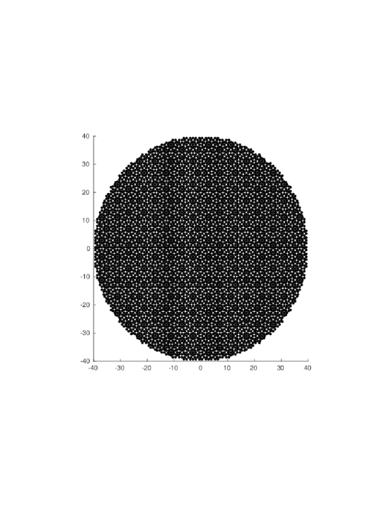
Figure 3.1. Round section of the quasilattice, of radius 40 lattice units.

For a given $\rho$, we will denote the Hamiltonian for the finite system on the round portion of the lattice centered at the origin of radius $\rho$ by $H_{\rho}$. We look also at Hamiltonians and round finite systems at other locations, but find these of little additional benefit and do not introduce notation for them.

We begin with an easy calculation, finding the norm of $H_{QC}$, which is just the largest eigenvalue. We remark that $H_{QC}$ has a form of particle-hole symmetry that is not of much interest here. It does tells us that all our eigenvalue calculations will be symmetric under the transformation $\lambda\mapsto-\lambda$. We will thus be able to focus on the eigenvalues that are zero or positive. It also allows us to find a unitary change of basis in some situations to transform a complex matrix into a real matrix. This leads to being able to work with slightly larger systems with the same computing hardware.

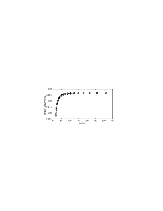
Figure 3.2. Norms of the compressed Hamiltonians $H_{\rho}$ as an estimator of the norm of $H_{QC}$ (solid line, round markers). Also computed for round portions of the same radii but centered at $(300,0)$ (dotted line, with plus markers) and also centered at $(-100,-200)$ (dashed line, with diamond markers).

The estimates on $\|H_{QC}\|$ look very similar if we locate the centers of the round portions at different locations. A manifestation of quasiperiodicity seems to be that for most calculations it matters little from where in the infinite quasilattice our finite lattices are taken. The conclusion we can make from the data in Figure 3.2 is $\|H_{QC}\|\approx 6.227$.

The expected edge states induced by the nonzero topological index will make finding the smallest eigenvalue more difficult than finding the largest eigenvalue. One strategy is to sort the eigenvalues into “bulk” and “edge” states by examining the associated states (eigenvectors). We arbitrarily declare a state to be an edge state if, according to its probability distribution, it is more than 50% likely to be observed to be outside of a circle of radius $\rho-3$, where $\rho$ is the radius of the finite system. We compute the integrated density of states, for positive energy only, and find many possible gaps beyond the expected gap at zero when looking at a small system of radius $\rho=15$. For $\rho=25$ there are still some small runs of edge states. See Figure 3.3.

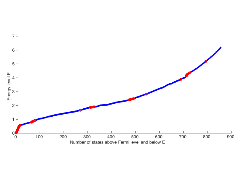
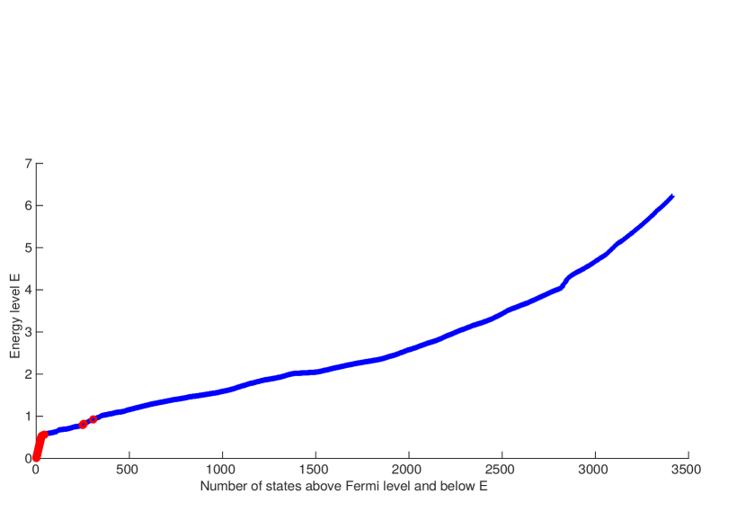
Figure 3.3. Integrated density of states, positive energy only. Each energy level is marked by a large, light, red circle if it corresponds to what seems to be a boundary mode, a small, dark, blue cross if corresponding to a bulk mode. Boundary mode is defined, rather arbitrarily, to correspond to the expectation of observing this mode within 3 lattice units of the boundary circle being at least $1/2$. Top panel is for radius 15. Bottom panel is for radius 25.

Looking at somewhat larger systems, up to $\rho=75$, we see in Figure 3.4 that the possible gap in the bulk spectrum near $E=0.8$ fades away. This is not a rigorous argument, and we can’t yet rule out small gaps in the bulk coming back at larger system size.

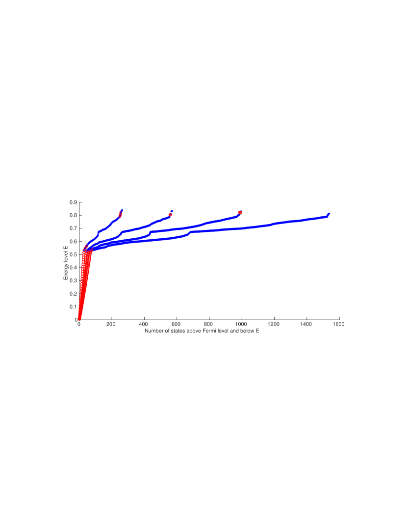
Figure 3.4. A portion of the IDOS. Radii 30, 45, 60 and 75 shown together.

States that are decidedly “bulk states” occur at many energies and system sizes. Two are illustrated in Figure 3.5. States that are decidedly “edge states” are common near zero energy, and two of these are illustrated in Figure 3.6.

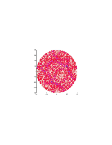
Figure 3.5. On the left the radius is 15, with eigenvalue $5.5066$. On the right the radius is 40 with eigenvalue $5.498$. Blue and dark dots are holes while red and lighter dots are particles. The area of each dot corresponds to the probability that this state is measured to be at that location.

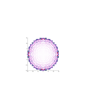
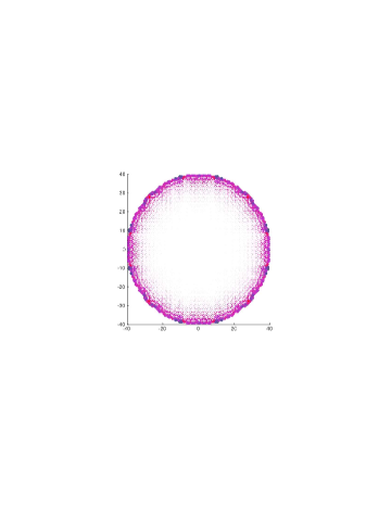
Figure 3.6. On the left the radius is 15, with eigenvalue $0.018$. On the right the radius is 40 with eigenvalue $0.007$.

What makes the situation complicated is the existence of states like those in Figure 3.7. At energy around $0.8$ we see some modes that are not really edge states and not really bulk states.

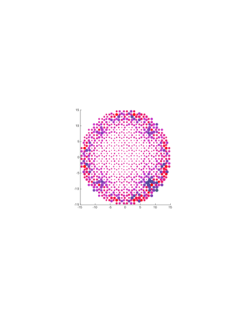
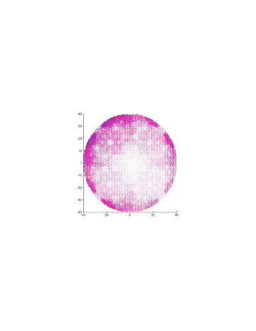
Figure 3.7. On the left the radius is 15, with eigenvalue $0.803$. On the right the radius is 40 with eigenvalue $0.828$.

One way to avoid such an ambiguous state is to work with a larger system, as in Figure 3.8. Unfortunately, we again find ambiguity with a yet larger system, as shown in Figure 3.9.

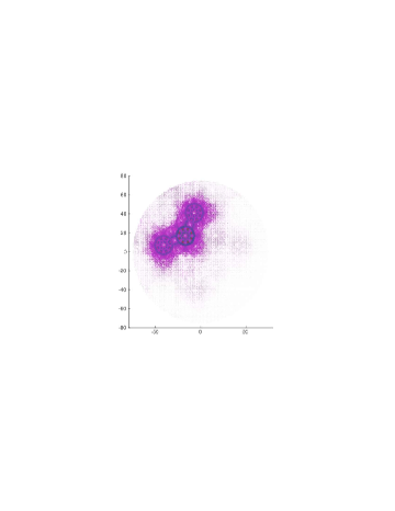
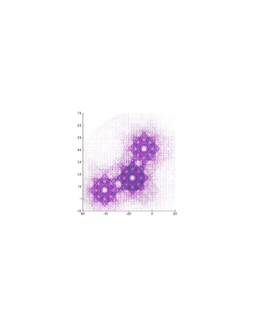
Figure 3.8. The eigenvector corresponding to $\lambda=0.831$ with radius 75. On the left the entire distribution. On the right, zoomed in to the densest portion.

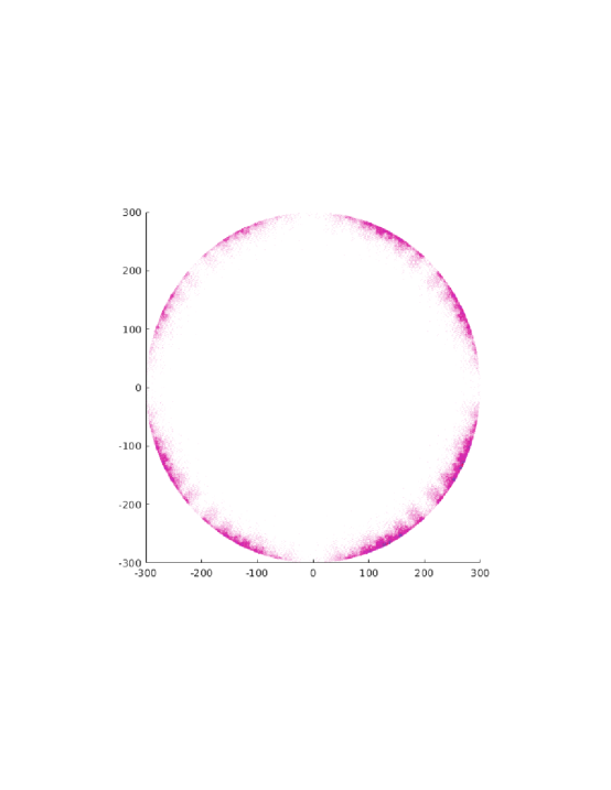
Figure 3.9. The eigenvector corresponding to $\lambda=0.828$ with radius $\rho=300$ is again ambiguous, a state somewhat on the edge.

4. Approximate Eigenvectors

To be more rigorous, we turn away from exact eigenvectors of a small Hamiltonian $H_{\rho}$ and investigate instead approximate eigenvectors of the full $H_{QC}$. Fortunately, the two concepts are related. As $H_{QC}$ is Hermitian, its spectrum equals its approximate point spectrum [13]. Moreover, every vector is close to a vector with support within a large circle at the origin. We say a vector $\psi$ on the Hilbert space for $H_{\rho}$ is zero at the boundary if it has value zero on all canonical basis element within one lattice unit of the bounding circle of radius $\rho$. If we pad $\psi$ with zeros, then the fact that $H_{\rho}$ has no hopping terms acting over a length more than $1$ means that

$$H_{QC}\left[\begin{array}[]{c}\psi\\ 0\end{array}\right]=\left[\begin{array}[]{c}H_{\rho}\psi\\ 0\end{array}\right].$$

All these facts constitute a proof that $\lambda$ is in the spectrum of $H_{QC}$ if, and only if, there is a sequence of vector states $\psi_{n}$ that are zero at the boundary in the truncated Hilbert space of radius $\rho_{n}$ such that

$$\lim_{n\rightarrow\infty}\left\|H_{\rho_{n}}\psi_{n}-\lambda\psi_{n}\right\|=0.$$

A more useful estimate can be obtain using Weyl’s estimate (see Bhatia’s book [9] for example) relating the spectrum of a perturbed Hermitian operator and the size of the perturbation. If we can produce a single state $\psi$ in the Hilbert space of radius $\rho_{n}$ that is zero at the boundary with

$$\left\|H_{\rho}\psi-\lambda\psi\right\|\leq\epsilon$$

then there is a point in the spectrum of $H_{QC}$ within distance $\epsilon$ of $\lambda$.

Given an eigenstate $\psi$ for $H_{\rho}$ with eigenvalue $\lambda$, we can multiply it by a tapering function, rescale the result to obtain $\psi^{\prime}$, and calculate the “eigenerror” $\left\|H_{\rho}\psi^{\prime}-\lambda\psi^{\prime}\right\|$ which is also a bound on the distance to the spectrum of the operator we care about, $H_{QC}$. This gets around the artificial dichotomy between bulk and edge states. Instead, we consider a state to be more concentrated in the bulk when the resulting eigenerror is smaller. This measure on bulkiness depends, of course, on our choice of taper function. We will use a radial function, where the scalar $\tau(r)$ used depends on the radius $r$ from the system center via

(4.1) $$\tau(r)=\begin{cases}1-\frac{2}{\rho_{1}^{2}}r{}^{2}&r<\frac{\rho_{1}}{2}\\ 1-\frac{2}{\rho_{1}^{2}}(r-\rho_{1})^{2}&\frac{\rho_{1}}{2}\leq r\leq\rho_{1}\\ 0&\rho_{1}<r\end{cases}$$

where $\rho_{1}=\rho-1$.

We call this method of producing approximate eigenvectors for $H_{QC}$ the compression method. This is because $H_{\rho}$ equals $\Pi_{\rho}H_{qc}\Pi_{\rho}$ on the appropriate subspace, where $\Pi_{\rho}$ is the projector onto the span of the canonical basis elements located within the circle of radius $\rho$. By looking for the eigenvalue of $H_{\rho}$ closest to every $\lambda$ in a grid, of increment $0.002$ between $E=0.6$ and $E=6.2$, and increment $0.05$ outside that interval down to $0$ and up to $7$, we find upper bounds on the distance to the spectrum as shown in Figure 4.1.

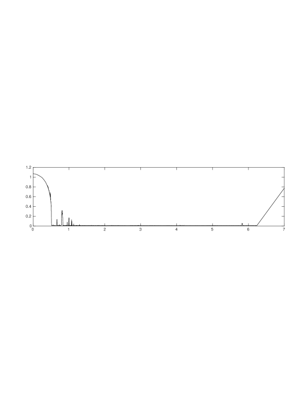
Figure 4.1. Upper bound on the distance to the bulk spectrum via approximate eigenvalues that were found by the compression method.

In this computation, it was necessary to use a radius as large as $\rho=691$. This corresponds to working on a Hilbert space of dimension $3,621,440$. As we need to work at many energy levels, this is a slow computation, and it turns out it is not so accurate. Figure 4.1 seems to indicate that there is a moderate gap in the bulk spectrum around $E=0.8$. We will see this is a mirage.

How we find approximate eigenvectors that are zero at the boundary is of no consequence as long as we compute the eigenerror. We hope that researchers in numerical linear algebra will look at this problem. In this work, eigensolvers are regarded as a black box, and the results are then manipulated to force zero at the boundary. It is expected that adapting an eigensolver to only consider vectors that are zero at and near the boundary will produce better results. This is out of the scope of this study, which is to illuminate methods physicists can immediately adopt.

5. Bulk Spectrum via the Spectral Localizer

The spectral localizer [21, 22] is designed to produce joint approximate eigenvalues for multiple observables. We will apply the spectral localizer to the observables $H_{\rho}-\lambda I$, $\kappa X_{\rho}$ and $\kappa Y_{\rho}$, where $X_{\rho}$ and $Y_{\rho}$ are the observables for position in the truncated round Hilbert space of radius $\rho$, where $\kappa$ is a tuning parameter, and $\lambda=E$ is one of the energy levels with which we are concerned. The spectral localizer in this case is

$$L=\left[\begin{array}[]{cc}H_{\rho}-\lambda I&\kappa X_{\rho}-i\kappa Y_{\rho}\\ \kappa X_{\rho}+i\kappa Y_{\rho}&-H_{\rho}+\lambda I\end{array}\right]$$

and we expect to find an eigenvalue for $L$ near $0$. Thus we have $\psi_{1}$ and $\psi_{2}$ with $\left\|\psi_{1}\right\|^{2}+\left\|\psi_{2}\right\|^{2}=1$ and

$$\left[\begin{array}[]{cc}H_{\rho}-\lambda I&\kappa X_{\rho}-i\kappa Y_{\rho}\\ \kappa X_{\rho}+i\kappa Y_{\rho}&-H_{\rho}+\lambda I\end{array}\right]\left[\begin{array}[]{c}\psi_{1}\\ \psi_{2}\end{array}\right]\approx\left[\begin{array}[]{c}0\\ 0\end{array}\right].$$

We then expect

$$H_{\rho}\psi_{j}\approx\lambda\psi_{j},$$

$$\kappa X_{\rho}\psi_{j}\approx 0$$

and

$$\kappa Y_{\rho}\psi_{j}\approx 0.$$

There is mathematics [22] predicting the accuracy of these approximations. However, these are generic estimates that don’t take into account the quasiperiodicity of $H_{QC}$, so they don’t deliver very useful bounds. In any case, we only care about the following. We rescale each $\psi_{j}$, so set

$$\psi_{j}^{\prime}=\frac{1}{\|\psi_{j}\|}\psi_{j},$$

and work with the $\psi_{j}^{\prime}$ with the smaller eigenerror

$$\left\|H_{\rho}\psi_{j}^{\prime}-\lambda\psi_{j}^{\prime}\right\|.$$

Finally, we apply the a taper function and rescale again,

$$\psi=\frac{1}{\left\|\tau(R)\psi_{j}\right\|}\tau(R)\psi_{j}$$

where $\tau$ is as in Equation 4.1 and $R=\sqrt{X_{\rho}^{2}+Y_{\rho}^{2}}$. This then gives an upper bound on

(5.1) $$\left\|H_{\rho}\psi_{j}-\lambda\psi_{j}\right\|$$

on the distance from $\lambda$ to the spectrum of $H_{QC}$.

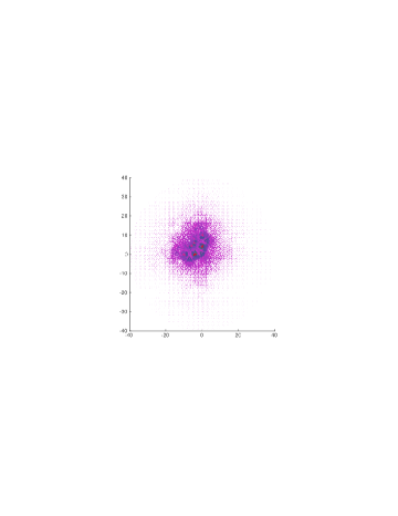
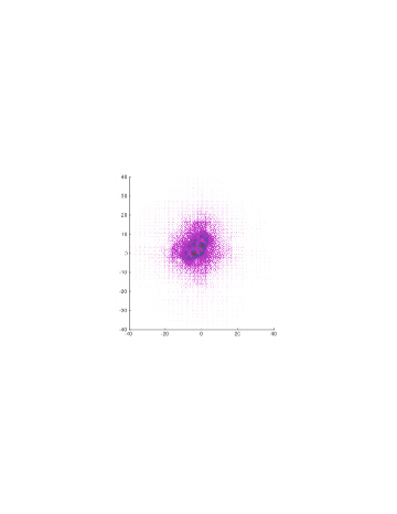
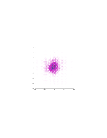
Figure 5.1. States produced by the localizer method with increasing values of $\kappa$ and with $\lambda$ set to $0.828.$ The top-left panel has $\kappa=0.0002$. The top-right panel has $\kappa=0.0010$. The bottom-left panel has $\kappa=0.0020$. The bottom-right panel has $\kappa=0.0050$.

Figure 5.2. Deviation of the states shown in Figure 5.1 with respect to $H_{\rho}$ and to radius $R_{\rho}=\sqrt{X_{\rho}^{2}+Y_{\rho}^{2}}$.

If we set $\kappa=0$ then this method reduces to the compression method, as both $\psi_{1}$ and $\psi_{2}$ will be exact eigenvectors for $H_{QC}$ for an eigenvalue near $\lambda$. In the case of $\lambda=0.828$ and $\kappa=0$ and radius $40$, the results will be exactly the state illustrated in Figure 3.7. Figures 5.1 and 5.2 illustrate the effect on the state found for the same $\lambda$ and $\rho$ but with increasing values for $\kappa$.

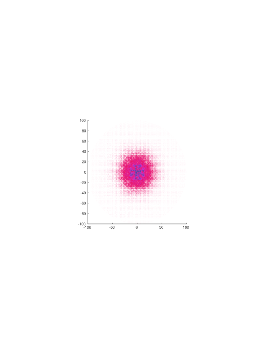
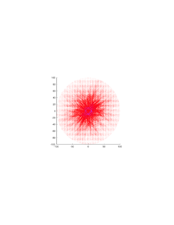
Figure 5.3. Approximate eigenvalues for the finite system, radius $100$. Found with the localizer method, with $\kappa=0.001$. On the top with approximate eigenvalue $0.66$. On the bottom with approximate eigenvalue $4.8$.

With the correct setting of the tuning parameter, we expect to get approximate eigenvectors for the finite Hamiltonian that are encouraged to live away from the boundary. We hope that the loss of accuracy incurred during the tapering process is enough smaller to compensate for the fact that we are starting with only an approximate eigenvector.

A few more of the approximate eigenvectors, before tapering, are shown in Figure 5.3. There are many energy levels to explore, which the reader is encouraged to explore with the software available as supplementary files [24].

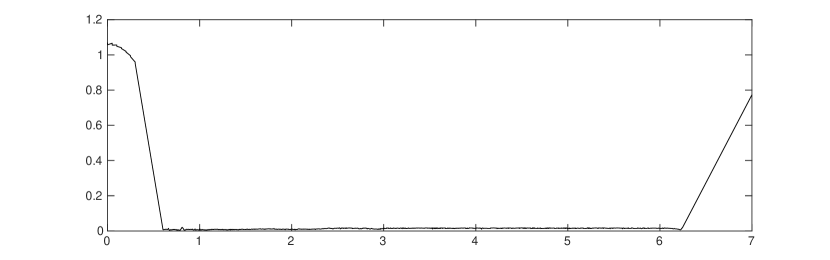
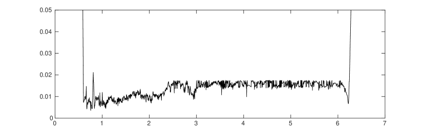
Figure 5.4. The top figure shows the upper bound on the distance to the bulk spectrum via approximate eigenvalues that were found by localizer method. The lower figure is zoomed in to clarify possible small gaps. The local peak at $\lambda=0.081$ was computed as approximately $0.021$. The left-most local minimum occurs at $\lambda=0.604$. The right-most local minimum occurs at $\lambda=6.222$.

We calculate upper bounds on the distance to the spectrum, on the same grid of energy values as with the compression method. We refer to this new method as the localizer method and the resulting upper bound on the distance to the bulk spectrum is shown in Figure 5.4.

We have thus computed the bulk spectrum to be contained in

$$[-6.227,-0.604]\cup[0.604,6.227]$$

and, if there is a gap within either of these bands, this gap will be of diameter at most $0.044$. There is some evidence, as in Figure 3.9 and Figure 5.4, that there is a pair of small gaps centered at about $\pm 0.82$.

The claim that there is no large gap in $[0.604,6.227]$ is solid, as its veracity rests only on the easy computation of the spectral errors in Equation 5.1. The claim that the top of the spectrum is roughly $6.227$ is a little less rigorously supported, as eigensolvers begin with a random seed and really bad luck can cause then to report a smaller eigenvalue than what is possible. The most speculative part of the claim is that the most inner eigenvalues are close to $\pm 0.604$. Making this a more rigorous claim will require new results about the spectral localizer when used in quasiperiodic conditions. It would make sense that someone do analytic work to get a solid estimate of the radius of this gap, which is $\left\|H_{QC}^{-1}\right\|^{-1}$. The advantage of the present method is it runs in only a few days on a computing cluster and should give an estimate in a reasonable time for other non-crystalline systems.

6. $K$-theory, Topological or $C^{*}$-Algebraic

There are two basic choices one can make when creating $K$-theoretical indices for phases of matter – to use topological $K$-theory or to use the $K$-theory of $C^{*}$-algebras. The later is essentially an extension of the former so it is more likely to apply. The ring structure on $K^{*}(X)$ is lost when looking at the $K$-theory of the $C^{*}$-algebra $C(X)$ but this is, so far, not of consequence in topological physics. Most particularly, when adding disorder it becomes more difficult to work with only topological $K$-theory. This observation goes back to the work of Bellisard [6]. We have lost translation invariance for a different reason and so also will utilize the $K$-theory of $C^{*}$-algebras.

As we have no symmetry of importance, we can work with the usual $C^{*}$-algebras, which are algebras over $\mathbb{C}$ with a particular sort of norm. The main examples are: the algebra $C(X)$ of continuous complex-valued functions on a compact Hausdorff space $X$; the finite-dimensional algebra $\boldsymbol{M}_{n}(\mathbb{C})$ for size $n$ square complex matrices; and the Caulkin algebra $\mathbb{B}(\mathcal{H})/\mathbb{K}(\mathcal{H})$ of bounded operators on Hilbert space modulo the compact operators. While $C(X)$ for $X$ a deformed sphere has a role in the mathematical proofs [21, 26] that relate finite volume and infinite volume indices, here its only role is motivational.

There are two groups associated to $A$, a $C^{*}$-algebra, denoted $K_{0}(A)$ and $K_{1}(A)$. Technically there is also $K_{2}(A)$, etc, but Bott periodicity [31] tells us $K_{2}(A)\cong K_{0}(A)$ and $K_{3}(A)\cong K_{1}(A)$, etc. It is also true that for a compact Hausdorff space $X$ there is an isomorphism $K_{j}(C(X))\cong K^{j}(X)$, so almost anything one can accomplish with topological $K$-theory can just as well be accomplished using the $K$-theory of $C^{*}$-algebras.

We first look at $K_{1}(A)$ for a $C^{*}$-algebra $A$ that we assume is unital. The usual picture of this in mathematics is built up from homotopy classes of unitary elements in $A$ and the matrices over $A$. An example, far older than the creation of $K$-theory, states that there is an isomorphism

$$\Psi:K_{1}\left(\mathbb{B}(\mathcal{H})/\mathbb{K}(\mathcal{H})\right)\rightarrow\mathbb{Z}$$

which is based on the index of a Fredholm operator that is essentially unitary:

$$\Psi(\left[T+\mathbb{K}(\mathcal{H})\right])=\mathrm{index}(T).$$

Because we are using complex scalars, our other example just ends up with $K_{1}\left(\boldsymbol{M}_{n}(\mathbb{C})\right)=0$. This reflects the elementary fact that any two unitary matrices of the same size can be connected by a continuous path of unitary matrices.

(Were we looking at real scalars, we would confront the fact that two real orthogonal matrices can be connected by a continuous path of real orthogonal matrices if and only if they have the same determinant. See [16, 22] on how some algorithms to compute indices of disordered 3D systems in class AII reduce to calculating the sign of the determinant of a large matrix.)

The classical construction of $K_{0}(A)$, again with $A$ a unital $C^{*}$-algebra, is in terms of projection in $A$ and the matrices over $A$. A familiar example involves the $C^{*}$-algebra

$$C(\mathrm{T}^{2},\boldsymbol{M}_{n})$$

of continuous functions from the torus to the $n$-by-$n$ matrices. A projection $P$ is required, by definition, so be self-adjoint with $P^{2}=P$. In this example, this means $P$ is a continuous function

$$P:\mathbb{T}^{2}\rightarrow\boldsymbol{M}_{n}$$

so that $P((\varphi,\theta))$ is the projector onto some continuously varying subspace of $\mathbb{C}^{n}$. This is exactly what one finds when looking at the Fermi projector in momentum space, when momentum space exists.

The example closer to the work here is $K_{0}\left(\boldsymbol{M}_{n}(\mathbb{C})\right)$. Any two projections in $\boldsymbol{M}_{n}(\mathbb{C})$ with the same multiplicity for $1$ are homotopic. Since we are allowed matrices over $\boldsymbol{M}_{n}(\mathbb{C})$, so $\boldsymbol{M}_{k}(\boldsymbol{M}_{n}(\mathbb{C}))$ which equals $\boldsymbol{M}_{kn}(\mathbb{C})$, we can achieve any positive multiplicity. We get an isomorphism

$$\Psi:K_{0}\left(\boldsymbol{M}_{n}(\mathbb{C})\right)\rightarrow\mathbb{Z}$$

which, for projection $P$, is defined by

$$\Psi\left([P]\right)=\dim(P(\mathbb{C}^{n})).$$

Of course, this is just the multiplicity of the eigenvalue $1$. To obtain a group we need “negative multiplicity” which arrives via the Grotendieck group construction that arguments the data we have with formal differences. So the full definition of $\Psi$ is

$$\Psi\left([P]-[Q]\right)=\dim(P(\mathbb{C}^{n}))-\dim(P(\mathbb{C}^{n})).$$

This traditional picture of $K_{0}$ and $K_{1}$ is elegant, but it is not ideal for numerical work. In practice, one comes across a Hermitian matrix with a gap in its spectrum, and to apply the traditional picture of $K$-theory one must compute a projection associated to that gap. This is computationally intense, and if one is to preserve sparsity one needs to accept $P^{2}\approx P$ anyway [8]. For some purposes, it is preferable to build $K_{1}(A)$ out of homotopy classes of invertible operators. For $K_{0}(A)$ we prefer to use homotopy classes of invertible Hermitian operators. Thus we are not using a gap at $\tfrac{1}{2}$ as one does implicitly when considering projections, but work with a gap at zero. This is also more compatible with various symmetries needed for real $K$-theory [11] or when working with class AII systems [16].

In this alternative picture of $K_{0}(A)$, for $A$ a unital $C^{*}$-algebra, we use homotopy classes of invertible Hermitian elements in $A$ and in matrices over $A$. To define the isomorphism

$$\Psi:K_{0}\left(\boldsymbol{M}_{n}(\mathbb{C})\right)\rightarrow\mathbb{Z}$$

it helps to use the signature. The signature $\mathrm{sig}(X)$ equals the number, counting with multiplicity, of positive eigenvalues of the given Hermitian matrix $X$ minus the number of negative eigenvalues. Then as long as $n$ is even, we define $\Psi$ by

$$\Psi\left([H]\right)=\frac{1}{2}\mathrm{sig}(H)$$

whenever $H$ is Hermitian and invertible.

7. Numerical $K$-Theory

The main theorem in prior work with Schulz-Baldes [21] tells us that the $K$-theory of a sufficiently large finite round system will equal that of the infinite system. For the infinite system there is no problem defining the $K$-theory class, or Chern number. On the infinite system we have the Hamiltonian $H_{QC}$ and position operators $X$ and $Y$. The Chern number is simply the index of a Fredholm operator

$$\mathrm{ind}(H_{QC},X,Y)=\mathrm{ind}\left(\Pi_{v}\left(\frac{X+iY}{\left|X+iY\right|}\right)\Pi_{v}+(I-\Pi_{v})\right)$$

on the full Hilbert space, and where $\Pi_{v}$ is the spectral projector of $H_{QC}$ corresponding to the valence band [7]. It is usually hopeless to use numerical algorithms to compute the index of a Fredholm operator, but in this case we rely on the spectral localizer and the previously derived estimates [21].

The version of in idex of the finite system we need here is based on the spectral localizer [22]. One forms the localizer at energy zero,

$$L_{\rho,\kappa}=\left[\begin{array}[]{cc}H_{\rho}&\kappa X_{\rho}-i\kappa Y_{\rho}\\ \kappa X_{\rho}+i\kappa Y_{\rho}&-H_{\rho}\end{array}\right],$$

and the index of the system $(H_{\rho},X_{\rho},Y_{\rho})$ is computed, with $\kappa$ at an appropriate value, as

$$\mathrm{ind}(H_{\rho},X_{\rho},Y_{\rho})=\frac{1}{2}\mathrm{sig}\left(L_{\rho,\kappa}\right).$$

This index is more robust, in terms of proven immutability under disorder up to a certain strength, when the localizer has a larger gap at the origin. It is equivalent to an element in the $K_{0}$-group of the $C^{*}$-algebra of bounded operators on the finite volume Hilbert space, or equivalently $K_{0}(\boldsymbol{M}_{n}(\mathbb{C}))$, as explained in Section 6.

We are guaranteed the equality

$$\mathrm{ind}(H_{\rho},X_{\rho},Y_{\rho})=\mathrm{ind}(H_{QC},X,Y),$$

according to the estimates obtained with Schulz-Baldes [21, Equation 5], when we have

$$\rho>\frac{24\left\|H_{QC}\right\|\left\|\left[H_{QC},X+iY\right]\right\|}{\left\|H_{QC}^{-1}\right\|^{-2}}.$$

We can get the estimate

$$\left\|\left[H_{QC},X+iY\right]\right\|\approx 3.583$$

by the same easy method used to estimate $\left\|H_{QC}\right\|$. We put in our estimates and find we need a radius of

$$\rho_{0}=1480.$$

We must (see Equation 6 in the paper with Schulz-Baldes [21]) select $\kappa_{0}$ in the range

$$\frac{2g}{\rho_{0}}<\kappa_{0}\leq\frac{\left\|H_{QC}^{-1}\right\|^{-3}}{12\left\|H\right\|\left\|\left[H,X+iY\right]\right\|},$$

meaning

$$0.000817\leq\kappa_{0}\leq 0.000821,$$

so we select

$$\kappa_{0}=0.0008175.$$

A radius of $1480$ leads to a Hilbert space of dimension of around $16.6$ million, so the localizer will be a matrix with over 33 million rows and column. It is sparse, but it is still annoyingly large. This is too large to compute on a single node of a computing cluster. Rather than resort to multi-node matrix factoring, we make a more modest numerical calculation and use a numerical computation of a homotopy to deduce that the signature of the huge localizer equals that of the more modest localizer. Thus we get a computer assisted calculation (not a fully rigorous proof) of what was surmised in prior work with Fulga and Piklin [14]:

$$\mathrm{ind}(H_{QC},X,Y)=-1.$$

Figure 7.1. Index for finite system of various radii and centers in the quasilattice. These results are for a very small value of the tuning parameter, $\kappa=0.0008175$, and a couple of larger values of $\kappa$.

What can be computed today using Matlab on a computer with 64GB of RAM is the signature of the localizer using radius of up to 600, which corresponds to Hilbert space of dimension about $2.7$ million. While not a proof, the data in Figure 7.1 is more compelling than what has been computed using the older formulas, such as the formula for the Bott index [25]. That index uses dense matrices, and cannot be used on today’s computers for systems with Hilbert space of dimension much larger than $20$ thousand. A common assumption about computing a Chern number is that the “various methods of computing it in real space” are “of similar computational efficiency” [28] but this seems to be false.

Notice that the data in Figure 7.1 is using the small tuning parameter $\kappa_{0}$ and somewhat larger values. For most purposes, a much larger value of $\kappa$ should be used, as has been done in numerical studies [14, 22]. The very small value of the tuning parameter is used here to accommodate the demands of the theorem we have [21] that relates finite systems to the infinite. The best way to set the tuning parameter is illustrated in Figures 5.1 and 5.2. When a $\kappa$ value causes the localizer to produce, on modest sizes systems, bulk states with deviation in energy noticeably smaller than the interesting gaps in the bulk, then that value of $\kappa$ should be valid for that system size. Keeping $\kappa$ fixed, or varying as $C/\rho$, when moving to larger systems leads to either a local or global $K$-theory index.

In order to relate a system of radius $\rho^{\prime}=600$ to one of radius $\rho_{0}=1480$, we consider two Hermitian matrices, $f_{0}(R_{\rho^{\prime}})H_{\rho^{\prime}}f_{0}(R_{\rho^{\prime}})$ and $f_{0}(R_{\rho_{0}})H_{\rho_{0}}f_{0}(R_{\rho_{0}})$ where

$$f_{0}(r)=\begin{cases}\left(1-\left(\frac{r}{\rho^{\prime}}\right)^{2}\right)^{\frac{1}{4}}&\text{if }r<\rho^{\prime}\\ 0&\text{if }r\geq\rho^{\prime}\end{cases}$$

and

$$R_{\rho}=\sqrt{X_{\rho}^{2}+Y_{\rho}^{2}}.$$

This function is the bottom one shown in Figure 7.2. Since $f_{0}(R_{\rho_{0}})$ takes value zero beyond radius $\rho^{\prime}$, the localizer for the larger system devolves, on the Hilbert space outside radius $\rho^{\prime}$, into a direct sum of many matrices of the form

$$\left[\begin{array}[]{cc}0&x-iy\\ x+iy&0\end{array}\right].$$

These have no effect on the signature, so

$$\mathrm{ind}(f_{0}(R_{\rho_{0}})H_{\rho_{0}}f_{0}(R_{\rho_{0}}),X_{\rho_{0}},Y_{\rho_{0}})=\mathrm{ind}(f_{0}(R_{\rho^{\prime}})H_{\rho^{\prime}}f_{0}(R_{\rho^{\prime}}),X_{\rho^{\prime}},Y_{\rho^{\prime}}).$$

We can compute the latter index numerically and we find

$$\mathrm{ind}(f_{0}(R_{\rho^{\prime}})H_{\rho^{\prime}}f_{0}(R_{\rho^{\prime}}),X_{\rho^{\prime}},Y_{\rho^{\prime}})=-1.$$

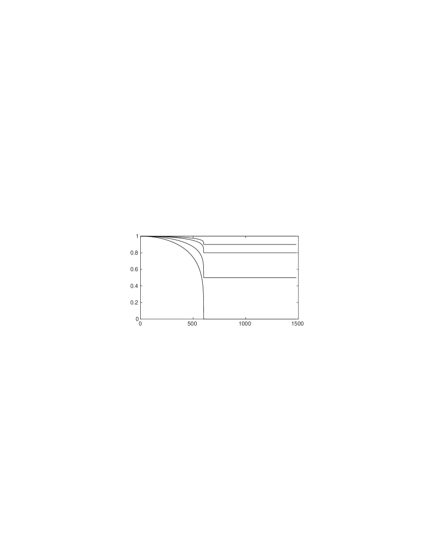
Figure 7.2. The tapering function $f_{0}$ and points along the homotopy to the constant function $f_{1}(r)=1$. Shown are $f_{t}$ for $t=0,0.5,0.8,0.9,1$.

To finish this argument we need to prove

(7.1) $$\mathrm{ind}(f_{0}(R_{\rho_{0}})H_{\rho_{0}}f_{0}(R_{\rho_{0}}),X_{\rho_{0}},Y_{\rho_{0}})=\mathrm{ind}(H_{\rho_{0}},X_{\rho_{0}},Y_{\rho_{0}})$$

which we do using the homotopy invariance of $K$-theory. We define

$$f_{t}(r)=(1-t)f_{0}(r)+t$$

as illustrated in Figure 7.2. Using this path of functions we now continuously connect $f_{0}(R_{\rho_{0}})H_{\rho_{0}}f_{0}(R_{\rho_{0}})$ to $H_{\rho_{0}}$ via

$$f_{t}(R_{\rho_{0}})H_{\rho_{0}}f_{t}(R_{\rho_{0}}).$$

If we can show that the resulting path of localizers

(7.2) $$\left[\begin{array}[]{cc}f_{t}(R_{\rho_{0}})H_{\rho_{0}}f_{t}(R_{\rho_{0}})&\kappa X_{\rho_{0}}-i\kappa Y_{\rho_{0}}\\ \kappa X_{\rho_{0}}+i\kappa Y_{\rho_{0}}&-f_{t}(R_{\rho_{0}})H_{\rho_{0}}f_{t}(R_{\rho_{0}})\end{array}\right]$$

remains invertible, we will be able to conclude that Equation 7.2 is true. This will then show

$$\mathrm{ind}(H_{\rho^{\prime}},X_{\rho^{\prime}},Y_{\rho^{\prime}})=-1$$

and so

$$\mathrm{ind}(f_{0}(R_{\rho^{\prime}})H_{\rho^{\prime}}f_{0}(R_{\rho^{\prime}}),X_{\rho^{\prime}},Y_{\rho^{\prime}})=-1.$$

That is, the infinite system is a Chern insulator.

Using analytic arguments, we are unable to show the path in Equation 7.2 is invertible. Such arguments [21] do work for paths of this form, but only for even larger systems. Since the path is at every point Hermitian, we can use Weyl’s estimate on spectral variation and a calculation at a fine grid of points that show the eigenvalue closest to $0$ is never very close to zero. We display the results of such a computation in Figure 7.3.

Figure 7.3. Distance of the spectrum to $0$, computed at 101 evenly spaced points along the path of localizers in Equation 7.2.

Each of the 101 points making the curve in Figure 7.3 was the result of estimating the eivenvalue closest to $0$ for an $N$-by-$N$ matrix $L$ where $N$ is approximately $33$ million. This is beyond the reach of basic eigensolvers. What was used here was the basic power method applied to a polynomial in $L$. The polynomial used is shown in Figure 7.4. This polynomial was selected to do a good job estimating, for Hermitian matrices of norm at most $7.4359$, the innermost eigenvalue if its absolute value is in the range $[0.1,1.5]$.

Figure 7.4. The polynomial applied to the localizer in the power method to estimate the innermost eigenvalue.

The implementation of this power method avoids matrix-matrix multiplication, working only with matrix-vector multiplication. This is rather standard numerical linear algebra, similar to some of the methods [20] used to estimate density of states when working with very large, sparse matrices. One expects a researcher trained in numerical linear algebra could do better, perhaps in the near future allowing us to determine the $K$-theory of an infinite quasicrystalline system in 3D.

8. Discussion

There are at least two notions of a local Chern number. There is the method [22] based on the spectral localizer or Clifford pseudospectrum. To make this truly a local marker we need to keep $\kappa$ rather large or fixed while the system size grows. Probably the first local Chern marker was introduce by Kitaev [19] and was generalized by Bianco and Resta [10].

A local Chern number can be used to differentiate bulk spectrum from edge spectrum in a finite sample. This strategy was employed in the study of a Chern insulator in an amorphous system [27]. Three-dimensional amorphous system appear to be capable of supporting topological behavior [1] many dimensions and symmetry classes which work with open systems, it should be possible to verify that this 3D amorphous system has nontrivial $\mathbb{Z}_{2}$ index, perhaps using available software [23].

Much work [15, 33] has gone into comparing the various ways to compute a (global) Chern number. It seems that now would be a good time for someone to systematically compare the values given by, and the computational complexity of, the various means of defining a local $K$-theory marker.

The reader might have expected a study involving larger finite samples of the Floquet topological insulator introduced by Bandres, Rechtsman and Segev [2]. What makes that system more challenging computationally is that a sparse time-dependent Hamiltonian could well lead to a dense Floquet Hamiltonian. Without sparsity, the localizer method for computing $K$-theory is not much more efficient than using the Bott index. It may be that good sparse approximations to the Floquet Hamiltonian exist, but calculating these is another challenge in the realm of numerical linear algebra.

It would be nice to approximately compute the density of states for $H_{QC}$ and related Hamilontians defined in terms of an infinite quasicrystal. It seems that the spectral localizer method and the methods used [20] to approximate the density of states for large but finite systems could be combined for this purpose. Alternately, one could try to prove that the local density of states for finite systems converges to something meaningful for an infinite system. Both paths are worth exploring, as a result on the density of states could somewhat make up for the lack of the momentum space band picture of topological insulators on quasilattices.

9. Supplementary Files

There are both data files and programs, all in Matlab formats, available as supplements [24] to this paper. The data files are large portions of the Ammann-Beenker quasilattice. The main program implements the compression and localizer method and displays the associated states.

References

- [1] Adhip Agarwala and Vijay B Shenoy, Topological insulators in amorphous systems, Phys. Rev. Lett. 118 (2017), no. 23, 236402.
- [2] Miguel A Bandres, Mikael C Rechtsman, and Mordechai Segev, Topological photonic quasicrystals: Fractal topological spectrum and protected transport, Phys. Rev. X 6 (2016), no. 1, 011016.
- [3] Siegfried Beckus and Jean Bellissard, Continuity of the spectrum of a field of self-adjoint operators, Ann. Henri Poincare, vol. 17, Springer, 2016, pp. 3425–3442.
- [4] Siegfried Beckus, Jean Bellissard, and Giuseppe De Nittis, Spectral continuity for aperiodic quantum systems i. general theory, J. Funct. Anal. 275 (2018), no. 11, 2917–2977.
- [5] Franciscus Petrus Maria Beenker, Algebraic theory of non-periodic tilings of the plane by two simple building blocks: a square and a rhombus, Eindhoven University of Technology Eindhoven, The Netherlands, 1982.
- [6] Jean Bellissard, -theory of -algebras in solid state physics, Statistical mechanics and field theory: mathematical aspects (Groningen, 1985), Lecture Notes in Phys., vol. 257, Springer, Berlin, 1986, pp. 99–156. MR 862832 (88e:46053)
- [7] Jean Bellissard, Andreas van Elst, and Hermann Schulz-Baldes, The noncommutative geometry of the quantum Hall effect, J. Math. Phys. 35 (1994), no. 10, 5373–5451.
- [8] Michele Benzi, Paola Boito, and Nader Razouk, Decay properties of spectral projectors with applications to electronic structure, SIAM review 55 (2013), no. 1, 3–64.
- [9] Rajendra Bhatia, Matrix analysis, vol. 169, Springer Science & Business Media, 2013.
- [10] Raffaello Bianco and Raffaele Resta, Mapping topological order in coordinate space, Phys. Rev. B 84 (2011), no. 24, 241106.
- [11] Jeffrey L. Boersema and Terry A. Loring, -theory for real -algebras via unitary elements with symmetries, New York J. Math. 22 (2016), 1139–1220. MR 3576286
- [12] Chris Bourne and Emil Prodan, Non-commutative Chern numbers for generic aperiodic discrete systems, J. Phys. A – Math. Theor. 51 (2018), no. 23, 235202.
- [13] Michael Demuth and Maddaly Krishna, Selfadjointness and spectrum, Determining Spectra in Quantum Theory (2005), 29–58.
- [14] Ion C Fulga, Dmitry I Pikulin, and Terry A Loring, Aperiodic weak topological superconductors, Phys. Rev. Lett. 116 (2016), no. 25, 257002.
- [15] Yang Ge and Marcos Rigol, Topological phase transitions in finite-size periodically driven translationally invariant systems, Phys. Rev. A 96 (2017), no. 2, 023610.
- [16] Matthew B. Hastings and Terry A. Loring, Topological insulators and -algebras: Theory and numerical practice, Ann. Physics 326 (2011), no. 7, 1699–1759.
- [17] Huaqing Huang and Feng Liu, Quantum spin Hall effect and spin Bott index in quasicrystal lattice, Phys. Rev. Lett. 121 (2018), no. 12, 126401.
- [18] by same author, Theory of spin Bott index for quantum spin Hall states in non-periodic systems, Phys. Rev. B 98 (2018), no. 12, 125130.
- [19] Alexei Kitaev, Anyons in an exactly solved model and beyond, Ann. Physics 321 (2006), no. 1, 2–111.
- [20] Lin Lin, Yousef Saad, and Chao Yang, Approximating spectral densities of large matrices, SIAM review 58 (2016), no. 1, 34–65.
- [21] Terry Loring and Hermann Schulz-Baldes, The spectral localizer for even index pairings, to appear in J. Noncommut. Geom., arxiv:1802.04517.
- [22] Terry A. Loring, -theory and pseudospectra for topological insulators, Ann. Physics 356 (2015), 383–416. MR 3350651
- [23] by same author, Pseudospectrum software, 2015, digitalrepository.unm.edu/math-statsdata/5/.
- [24] by same author, Supplemental material, 2018, www.math.unm.edu/%7Eloring/Localizer/.
- [25] Terry A Loring and Matthew B Hastings, Disordered topological insulators via C*-algebras, EPL (Europhysics Letters) 92 (2011), no. 6, 67004.
- [26] Terry A. Loring and Hermann Schulz-Baldes, Finite volume calculation of -theory invariants, New York J. Math. 23 (2017), 1111–1140. MR 3711272
- [27] Noah P Mitchell, Lisa M Nash, Daniel Hexner, Ari M Turner, and William TM Irvine, Amorphous topological insulators constructed from random point sets, Nat. Phys. 14 (2018), 380–385.
- [28] Kim Pöyhönen, Isac Sahlberg, Alex Westström, and Teemu Ojanen, Amorphous topological superconductivity in a Shiba glass, Nat. Commun. 9 (2018), no. 1, 2103.
- [29] Emil Prodan and Hermann Schulz-Baldes, Bulk and boundary invariants for complex topological insulators, Mathematical Physics Studies, Springer, [Cham], 2016, From -theory to physics. MR 3468838
- [30] Przemysław Repetowicz, Uwe Grimm, and Michael Schreiber, Exact eigenstates of tight-binding Hamiltonians on the Penrose tiling, Phys. Rev. B 58 (1998), no. 20, 13482.
- [31] M. Rørdam, F. Larsen, and N. Laustsen, An introduction to -theory for -algebras, London Mathematical Society Student Texts, vol. 49, Cambridge University Press, Cambridge, 2000. MR MR1783408 (2001g:46001)
- [32] C Sire and J Bellissard, Renormalization group for the octagonal quasi-periodic tiling, EPL (Europhysics Letters) 11 (1990), no. 5, 439.
- [33] Daniele Toniolo, On the equivalence of the Bott index and the Chern number on a torus, and the quantization of the Hall conductivity with a real space kubo formula, arXiv preprint arXiv:1708.05912 (2017).
- [34] Duc-Thanh Tran, Alexandre Dauphin, Nathan Goldman, and Pierre Gaspard, Topological Hofstadter insulators in a two-dimensional quasicrystal, Phys. Rev. B 91 (2015), no. 8, 085125.
- [35] Hirokazu Tsunetsugu, Takeo Fujiwara, Kazuo Ueda, and Tetsuji Tokihiro, Electronic properties of the Penrose lattice. I. energy spectrum and wave functions, Phys. Review B 43 (1991), no. 11, 8879.