Evaluation of the Vertical Scale Height of L dwarfs in the Galactic Thin Disk

Abstract

Using the data release 1 of the Hyper Suprime-Cam Subaru Strategic Program covering about 130 square degrees at high galactic latitudes, we have obtained L dwarf counts based on the selection criteria on colors, limiting magnitude and PSF morphology using $i$, $z$, and $y$ bands. 3665 L dwarfs brighter than $z=24$ have been detected by these criteria. The surface number counts obtained differentially in $z$ magnitude are compared with predictions of an exponential disk model to estimate the thin-disk scale height in the vicinity of the Sun. In the exponential disk model, we first fix the local luminosity function (LLF) to the mean LLF of Cruz et al. (2007) and derive the best fit scale height of 260 pc. However this fit appears to be poor. We then allow the LLF to vary along with the scale height. We use the LLF of Cruz et al. as a starting point. The best-fit model is found for the vertical scale height of 380 pc. However the $\chi^{2}$ minimum is rather broad and the 90% confidence interval is between 320 and 520 pc. We investigate another model by varying the scale height and the density of the brightest magnitude bin, while other magnitude bins are fixed to the mean LLF of Cruz et al.. We find an equally good fit with the two free parameters and the best-fit scale height is again 380 pc, but the 90% confidence interval is between 340 and 420 pc.

1 Introduction

The statistical study on the brown dwarf population has become possible by the advent of the large-area digital surveys such as the Two Micron All Sky Survey (2MASS: Skrutskie et al. (2006)), Sloan Digital Sky Survey (SDSS: York et al. (2000)), Canada-France brown dwarf survey and its infrared version, (CFBDS & CFBDSIR: Delorme et al. (2010)), UKIRT Infrared Deep Sky Survey (UKIDSS: Lawrence et al. (2007)) and a space-based all-sky survey by the Wide-field Infrared Survey Explorer (WISE: Wright et al. (2010)). Utilizing the data from these large-area surveys, several groups have determined the number densities of various types of brown dwarfs in the solar neighborhood, or more precisely the local luminosity function (LLF) of the brown dwarfs (Cruz et al., 2007; Metchev et al., 2008; Reylé et al., 2010; Kirkpatrick et al., 2012; Day-Jones et al., 2013; Burningham et al., 2013; Marocco et al., 2015).

Beyond the immediate solar neighborhood, brown dwarfs are expected to have density distribution similar to the stars in our Galaxy. In other words, brown dwarfs will have thin-disk, thick-disk and halo populations, as stars do. However, the determination of the spatial distribution of brown dwarfs in the context of the Galactic structure is not an easy task because of their faintness. In fact even the spatial distribution of low mass stars, which are a little more massive than brown dwarfs, has been determined only recently. The vertical scale height of low mass stars has been estimated by the analyses of the SDSS data by several studies (Chen et al., 2001; Jurić et al., 2008; Bochanski et al., 2010). The derived scale height ranges from 290 to 330 pc. The M dwarf scale height has been obtained also by the analyses of the HST data (Pirzkal et al., 2009; van Vledder et al., 2016) and it ranges from 290 to 370 pc. These results from SDSS and HST should be compared with the spatial distribution of brown dwarfs.

The previous ground-based surveys are not deep enough to detect brown dwarfs as far as 300 pc, which is roughly the scale height of low mass stars. Only data that reach beyond 300 pc, are obtained by the HST, whose pencil beam surveys have picked up rather small numbers of brown dwarfs, but have given estimates of the vertical scale height, which range from 290 to 400 pc (Pirzkal et al., 2005; Ryan et al., 2005, 2011).

The Hyper Suprime-Cam Subaru Strategic Program (HSC-SSP) survey is capable of detecting a large number of new brown dwarfs because of a greater limiting distance and a larger volume for a given spectral type compared with previous surveys. In this paper, we report the number count of new color-selected L dwarfs using the HSC-SSP survey data and discuss the vertical distribution of L dwarfs in the Galactic thin disk.

Our paper is organized as follows. In section 2, we provide the information on HSC-SSP data and L dwarf selection in our analysis. In section 3, we show the results of comparison of the magnitude dependent number counts of L dwarfs obtained from the HSC-SSP data and predictions of an exponential disk model. In section 4, our results are compared with the previous works on brown dwarfs and low mass stars.

2 Data and L Dwarf Selection

2.1 HSC DR1 Data

HSC is a new prime-focus camera mounted on the 8.2 m Subaru telescope (Miyazaki et al., 2018). Compared with the Suprime Cam, the prime-focus imager of the previous generation, the field of view (FOV) of the HSC is ten times larger, while it is less affected by distortion. HSC has 104 red-sensitive science CCDs whose 870 Mega pixels cover 1.5 degree diameter FOV with a 0.168 arcsec pixel scale. HSC-SSP, which is led by the astronomical communities of Japan, Taiwan, and Princeton University, is carrying out a multi-band ($g,r,i,z$, and $y$ broad bands, and 4 narrow-band filters) imaging survey. The survey consists of three layers with different depths: wide, deep and ultra-deep. We use 130 square degrees of the data release 1 (DR1) of the wide and deep surveys, which was released in February 2017 (Aihara et al., 2018).

Several astronomical surveys related to brown dwarf research have been carried out so far. The representative ground-based surveys are 2MASS (Skrutskie et al., 2006), SDSS, (York et al., 2000), CFBDS & CFBDSIR, (Delorme et al., 2010), UKIDSS (Lawrence et al., 2007), Visible and Infrared Survey Telescope for Astronomy (VISTA) Kilo-Degree Infrared Galaxy Survey and Hemisphere Survey (VIKING & VHS: Arnaboldi et al. (2007)). There is also a space-based all-sky survey, WISE (Wright et al., 2010).

Table 1: Comparison of limiting distances and survey volumes

survey	SpT	$M_{z}$	limiting $z$ mag	$M_{J}$	limiting $J$ mag	limiting $d$	survey area	volume
						[pc]	[deg2]	[pc3]
HSC	L5	16.4	24.3	–	–	378	1400	$7.70\times 10^{6}$
HSC	T6	17.8	24.3	–	–	196	1400	$1.07\times 10^{6}$
SDSS	L5	16.1	20.0	–	–	60	10000	$2.19\times 10^{5}$
SDSS	T6	17.5	20.0	–	–	31	10000	$3.04\times 10^{4}$
CFBDS	L5	16.1	22.5	–	–	190	600	$4.16\times 10^{5}$
CFBDS	T6	17.5	22.5	–	–	98	600	$5.76\times 10^{4}$
CFBDSIR	L5	–	–	13.8	20.0	177	335	$1.89\times 10^{5}$
CFBDSIR	T6	–	–	15.1	20.0	97	335	$3.09\times 10^{4}$
UKIDSS	L5	–	–	13.8	19.3	128	4000	$8.56\times 10^{5}$
UKIDSS	T6	–	–	15.1	19.3	70	4000	$1.40\times 10^{5}$
VHS	L5	–	–	13.8	19.4	134	20000	$4.92\times 10^{6}$
VHS	T6	–	–	15.1	19.4	73	20000	$8.05\times 10^{5}$
VIKING	L5	–	–	13.8	20.4	213	1500	$1.47\times 10^{6}$
VIKING	T6	–	–	15.1	20.4	116	1500	$2.40\times 10^{5}$
2MASS	L5	–	–	13.8	15.8	26	40000	$6.80\times 10^{4}$
2MASS	T6	–	–	15.1	15.8	14	40000	$1.11\times 10^{4}$

Note. — Limiting magnitudes are given for 10-sigma significance. $z$ magnitude is in the AB system, while $J$ magnitude is in the Vega system. $M_{z}$ and $M_{J}$ are from Filippazzo et al. (2015). $M_{z}(hsc)-M_{z}(SDSS)=0.3$ (This paper).

We summarize the 10-sigma limiting magnitudes of $z$ band for HSC, SDSS, and CFBDS, and of $J$ band for 2MASS, UKIDSS, CFBDSIR, VHS and VIKING, limiting distances in units of pc, survey areas in units of deg², and volumes in units of pc³ for L5 and T6 dwarfs in Table 1. WISE is sensitive at 4.6 $\mu$m and main targets are late T and Y dwarfs within 10 pc of the Sun (Kirkpatrick et al., 2011) and therefore we have excluded WISE from this comparison. Figure 1 shows the limiting distances and survey volumes for L5 and T6 dwarfs for different surveys. For L5 dwarfs, HSC is the only survey that reaches more than 300 pc, which is approximately the scale height of M dwarfs. VIKING is the runner-up, while the volume covered by VHS will be comparable to that covered by HSC at the time of their completion. For T6 dwarfs, HSC reaches almost 200 pc and VIKING is again in the second place ($\sim$ 120 pc), though neither of the surveys reaches 300 pc, which is about the necessary limiting distance to obtain a scale height.

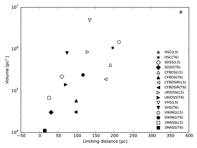
Figure 1: The limiting distances and volumes for L5 and T6 dwarfs for different surveys. For L5 dwarfs, the HSC survey is the only survey that reaches beyond 300 pc, which is about the scale height of M dwarfs.

2.2 Deep and Wide fields

We use three fields of the Deep layer and six fields of the Wide layer. The name and properties of each field are given in Table 3. The major difference between the Deep and Wide fields is that narrow-band filters were used in addition to broad-band filters in the Deep layer. As far as broad-band imaging is concerned, the difference in depth in each band is 0.1 mag (Aihara et al., 2018), which is much smaller than 0.42 mag, which is the uncertainty in the absolute $z$ mag of L dwarfs, which appears in model fitting procedure (Section 3). The survey areas of the Wide fields in general are greater than those of the Deep fields, but there is one exception, HECTOMAP (Wide), whose survey area is smaller than those of the three Deep fields. For these reasons, we treat all nine fields in the same manner in the following analysis.

It should be emphasized that the above statements regarding the depth of the Deep survey and the width of HECTOMAP are strictly true for the DR1 release, since the surveys are still on-going. At the time of completion, the Deep survey will be much deeper and the area of HECTOMAP will be much wider.

2.3 Selection conditions

We first choose data sources from the HSC-SSP DR1 database for non-blended sources satisfying the following conditions:

1. $S/N>10$ in $z$

2. $1.0<i-z<2.0$

3. $0.75<z-y<1.0$

4. $z-z_{cModel}<0.15$

where $i,z$, and $y$ are in the AB magnitude system. Here magnitudes of the HSC data refer to point-spread function (PSF) magnitudes. $z_{cModel}$ is measured by fitting the PSF-convolved galaxy models to the source profile. The difference between the PSF and $cModel$ magnitudes is used to exclude extended sources.

In addition, we use the following critical quality flags, which are used in Matsuoka et al. (2016, 2018a, 2018b): we require that the source (i) is not close to an edge of the image frame (flags$\_$pixel$\_$edge = False), (ii) is not in a bad CCD region (flags$\_$pixel$\_$bad = False), (iii) is not saturated (flags$\_$pixel$\_$saturated$\_$center = False), (iv) is not affected by cosmic rays (flags$\_$pixel$\_$cr$\_$center = False) in the $i$, $z$, and $y$ bands, (v) does not include a footprint in bright object pixels (zflags$\_$pixel$\_$bright$\_$object$\_$center = False). Below we discuss the implications of each selection criterion.

2.4 L dwarf selection

Condition 1.

$z$ band is the primary band where the observed and model counts are compared in section 3. This condition for the S/N is effectively equivalent to $z<24$ and $\sigma_{z}<0.1$ mag. The photometric uncertainty of $\sigma_{z}<0.1$ is much smaller than the intrinsic scatter of the absolute $z$ magnitude of the L dwarfs of 0.42 mag, which we derive in section 3. Interstellar extinction of the observed fields ranges from $A_{z}=0.03$ to 0.09 (Schlafly & Finkbeiner, 2011), which is again much smaller than the intrinsic scatter of the absolute $z$ magnitude of L dwarfs. So we neglect the effect of interstellar extinction from our analysis. We consider that the observed L dwarf count is complete to $z=24$ as we show in section 2.5.

Conditions 2 & 3.

Figure 2 shows the $i-z$ vs. $z-y$ diagram for known M dwarfs (red), M9 dwarfs (cyan), and L dwarfs (blue). The $i-z$ and $z-y$ colors of these dwarfs are synthesized from the HSC filter functions of $i$, $z$, and $y$ bands for spectra obtained with SpeX, a medium-resolution spectrograph covering 0.65–5.4 $\mu$m at the NASA Infrared Telescope Facility (IRTF), and CGS4, a cassegrain spectrograph at the United Kingdom Infrared Telescope (UKIRT). These colors of known brown dwarfs are derived by Matsuoka et al. (2016, 2018a, 2018b).

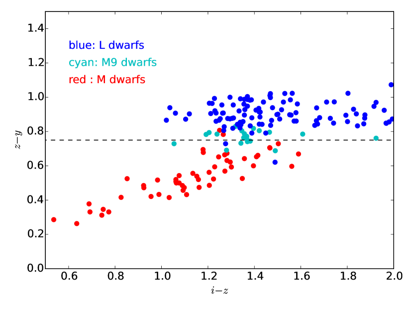
Figure 2: The $i-z$ vs. $z-y$ diagram. The known M($\leq 8$), M9(including M8.5), and L dwarfs are shown in red, cyan, and blue points, respectively. The M8/M9 border ($z-y$ = 0.75) is shown in black dashed line. This border is selected so that early L dwarfs are included even if some of the M9 dwarfs are also included.

$i-z=1.0$ is the blue border of L dwarfs, while $i-z=2.0$ is almost the red border of L dwarfs. It should be noted that the $z(hsc)$ filter transmits rather shorter wavelengths than the $z^{\prime}(SDSS)$ filter, since the $y$-band is used as the longest wavelength band. In Figure 1 of Matsuoka et al. (2016), an $i-z$ vs $z-y$ digram is plotted for wider ranges of $i-z$ and $z-y$. According to this figure, L/T transition occurs around $i-z\sim 2.5$ and we exclude the latest L dwarfs (roughly L9) and L/T transition objects by the criterion $i-z<2.0$. The reason for the exclusion of L9 and later dwarfs is that our L dwarf count should be consistent with the local luminosity function (LLF) we use of Cruz et al. (2007), which includes L dwarfs down to L8, but does not include L9 and L/T transition objects.

Compared with the L/T border, the M/L border is more problematic. We set $z-y=0.75$ as an M/L border around which M/L transition objects are mixed up. We can see that almost all of the M-type objects included in the M/L mixed zone around $z-y\sim 0.75$ are M9(and M8.5) dwarfs. Since it is intrinsically difficult to determine the spectral class for the M/L borderline objects, we regard $z-y=0.75$ as an M8/M9 border. So we allow M9 dwarfs to be included in the L dwarf sample, while we avoid excluding early L dwarfs from the L dwarf sample. M9 dwarfs are taken into account in the brightest magnitude bin of the LLF of Cruz et al. in section 3.

2.5 Completeness

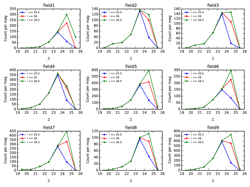
Figure 3: $z$ band source counts are compared for $i<25.5,26.0$ and $26.5$ for each of the nine fields. The three source counts for each field do not differ one another down to $z=23.5$ or (23-24) bin. These results combined with the color criterion $i-z<2.0$ indicate that our sample is complete to $z=24$. The names of the fields are given in Table 3.

Since $i-z<2.0$, the faintest and reddest object at $i$ selected by the criterion $z<24$ is $i=26$. In Figure 3, differential source counts per $z$ magnitude for all nine fields that satisfy the selection criteria are plotted for $i<25.5,26.0$ and 26.5. The source counts of the three cases agree reasonably well down to $z=23.5$ or (23-24) bin, while they deviate from $z=24.5$. It is essential that the source counts agree down to $z=23.5$ for $i=26$ and $i=26.5$. From $z-y>0.75$ and $z<24$, $y<23.25$ for which S/N $>8$, and the sources at $y$ band have higher S/N than at $i$ band. From the interpretation of Figure 3, we confirm that the source counts are complete to $z=24$ for $i-z<2.0$.

Another potential source of incompleteness is the seeing dependence of the point-source selection condition 4, $z-z_{cModel}<0.15$. Seeing variation exists among different fields and also within a field. In their high-redshift quasar survey, Matsuoka et al. (in preparation) investigated the magnitude dependent completeness due to the point-source selection, taking into account the seeing variation. According to their formula, the completeness was 99 and 95% respectively at $z=22.5$ and 23.5, regardless of seeing. In the model fitting procedure described in Section 3, we compared the case for raw observed counts and that for completeness corrected counts. It was found that the effect of correction was not negligible at the level of 20 pc difference in the scale height. So we included completeness correction due to point-source selection.

2.6 Potential contaminants

2.6.1 L subdwarfs

In this paper, we consider only thin disk population of L dwarfs and we neglect thick disk and halo populations of L dwarfs, or so called L subdwarfs (sdL). To justify our approach, here we estimate the contribution of L subdwarfs in two ways.

$i-z$ and $z-y$ colors of L subdwarfs are not known, but we assume that all L subdwarfs satisfy our color criteria and estimate an upper limit of L subdwarf contribution. $r-z$ color of subdwarf M8 is known to be $\sim$ 2.8 (Lépine & Scholz, 2008) and we assume that $r-z\sim 3$ for sdL0. Lodieu et al. (2017) surveyed 3700 deg² of SDSS and UKIDSS data down to $r\sim 23$ or approximately $z\sim 20$, and detected 3 L subdwarfs (two sdL0 and one sdL0.5). In terms of surface number density, this corresponds to 8.1$\times 10^{-4}$ per deg². If we estimate the surface number density for the HSC limit of $z=24$, it will be 0.21 per deg². If we apply the completeness correction as Lodieu et al did, the surface number density increases to 0.51 per deg². For our survey area of some 130 deg², we expect an upper limit of 66 L subdwarfs which is less than 2% of our total L dwarf count. We consider this contribution to be negligible.

Since Lodieu et al. (2017) detected only very early L subdwarfs, one may worry about the contribution of L subdwarfs of later spectral type. About the entire L subdwarf population, some hint can be obtained from the result of the ALLWISE sky survey by Kirkpatrick et al. (2014). According to Table 6 of their paper, the volume number density in the immediate solar neighborhood of L subdwarfs can be estimated to be about 0.3% of that of thin disk L dwarfs. If we move out of the Galactic plane by one exponential scale height, the fraction will increase to 0.9%, but this fraction is still small. Again we conclude that L subdwarf population is negligible.

2.6.2 Passive elliptical galaxies at z $\sim 1$

Passively evolving elliptical galaxies at z(redshift)$\sim 1$ have large $i-z$ colors due to the 4000Å break in the rest-frame SEDs. Yamada et al. (2005) detected about 4000 such objects (z=0.9 $\sim$ 1.1) in 1.03 deg² of the Subaru/XMM-Newton Deep Survey, which are brighter than $z^{\prime}<25$ using the Suprime Cam, the predecessor of HSC. There may be more than 1000 passively evolving elliptical galaxies brighter than $z=24$ per deg², which satisfy $i-z$ color criterion. If selection criteria other than $i-z>1.0$ could not reject these galaxies, they would outnumber L dwarfs.

Here we argue that the color criterion $z-y>0.75$ efficiently excludes these galaxies based on the following reasoning. At z$\sim 1$, the rest-frame wavelengths of $z$ and $y$ are 4400 and 4800Å respectively. The rest-frame SEDs of passive elliptical galaxies of various ages and metallicities are found in Barbaro & Olivi (1989). The ratio of rest-frame flux densities $f_{\nu}(4400)/f_{\nu}(4800)$ ranges from 1.07 to 0.83 from the most metal poor to the extremely metal rich case. Since the color in AB magnitude is effectively the ratio of the flux densities, which is preserved even if the redshift is changed, $z-y$ ranges from -0.07 to 0.2.

Now we consider if the intrinsically reddest galaxy with $z-y=0.2$ accidentally has $z-y>0.75$ due to photometric errors in $z$ and $y$. The reddest and faintest galaxy will have the intrinsic $z=23.25$ and $y=23.0$. 1 sigma photometric errors for this galaxy are 0.05 and 0.1 respectively for $z$ and $y$ and corresponding 1 sigma error in $z-y$ is 0.11. Since $z-y=0.75=0.2+5\times 0.11$, the photometric error in $z-y$ needs to exceed 5 sigma level in order to contaminate L dwarfs. It should be emphasized that intrinsic $z-y$ of most of the galaxies is less than 0.2. Passive elliptical galaxies at z$\sim 1$ are not likely to be as red as L dwarfs in $z-y$.

In addition to the $z-y$ color criterion, the PSF criterion (condition 4) discussed in Section 2.5, is efficient in excluding passive elliptical galaxies which are expected to be extended. This is another reason that passive elliptical galaxies are not significant contaminants.

2.6.3 High-redshift quasars and high-redshift galaxies

Since Matsuoka et al. (2016, 2018a) conducted a high redshift quasar survey using the HSC-SSP Wide Survey data based on color-color selection criteria similar to ours, their results are most relevant to our analysis.

In Figure 1 of Matsuoka et al. (2016), they plot in the $i-z$ vs $z-y$ diagram the loci of high-redshift quasars and high-redshift galaxies as well as the locations of L and T dwarfs. In this color-color diagram, quasars and galaxies overlap with L dwarfs for only a narrow range of z(redshift) $\sim 6.5$. In this redshift interval, the expected number of quasars with $z<24$ is a few in 130 deg² and that of galaxies which appear to be point like in HSC images is also a few in 130 deg² (Matsuoka et al., 2016, 2018a, 2018b). These results imply that both quasars and galaxies are negligible for our L dwarf count.

We have finally extracted a total of 3665 sources in which only a very small fraction of objects are expected to be non thin-disk L dwarfs.

3 L dwarf distribution in the Galactic disk

3.1 Exponential disk model

3.1.1 Thin disk model

Here we consider only the thin disk population by an exponential disk model. The number density of the L dwarfs of the $k$ th magnitude bin of the $J$ band luminosity function at the Galactic position $(R,Z)$ in cylindrical coordinates, is given by

$$\Phi_{k}(R,Z)=\Phi_{k}\exp\left(\frac{R_{0}-R}{H}-\frac{|Z|}{h}\right),$$ (1)

where $\Phi_{k}$ is the number density of the $k$ th magnitude bin of the $J$ band local luminosity function (LLF) of the L dwarfs of the immediate solar neighborhood, $R_{0}=8$ kpc is the Galactocentric distance, $H=3.5$ kpc is the Galactic scale length, and $h$ is the vertical scale height to be estimated from the comparison of the model and observations. We start from $J$-band because a L dwarf LLF has been obtained previously at $J$ band by Cruz et al. (2007). The range of absolute $J$ magnitude is from 11.75 to 14.75 with a 0.5 mag step, covering in spectral type from M9/L0 to L8. In the calculation of the surface number density in the line of sight of the Galactic coordinates $(l,b)$, the height of the Sun above the Galactic plane, $Z_{\odot}=27$ pc (Chen et al., 2001) is taken into account.

3.1.2 Error in $z$-band absolute magnitude

The absolute $J$ magnitude is converted to absolute $z(hsc)$ magnitude by the $z(SDSS)-J$ vs. $M_{J}$ relation (Filippazzo et al., 2015) and $z(hsc)-z(SDSS)=0.3$ which we derived. The relation between $M_{J}$ and $z(hsc)-J$ is given in Table 2. The uncertainty involved in this conversion is estimated to be 0.3 mag.

In the work of Cruz et al., the uncertainty in spectral type is a half subtype, which induces an uncertainty of 0.3 mag in $M_{J}$. Assuming that the error in the color conversion and that in $M_{J}$ are independent, the total error in the absolute $z$ mag amounts to 0.42 mag, which causes significant Malmquist bias. Photometric error is less than 0.1 mag and this contribution is small compared with the error in $M_{z}$. In Appendix, our treatment of Malmquist bias following the original procedure adopted by Malmquist (1922) is given. The only difference in our case is that we used numerical integration in apparent $z$ magnitude which is usable for any form of the density distribution, while Malmquist used analytic integration for the cases it is possible (The famous formula for example is for a uniform density distribution).

$M_{J}$	11.75	12.25	12.75	13.25	13.75	14.25	14.75
$z(hsc)-J$	2.25	2.40	2.52	2.61	2.65	2.70	2.75

Table 2: $M_{J}$ vs. $z(hsc)-J$ . $M_{J}$ vs. $z(SDSS)-J$ relation was obtained from Filippazzo et al. (2015) and $z(hsc)-z(SDSS)=0.3$ was derived by us. The uncertainty in this color-magnitude relation induces 0.3 mag uncertainty in $M_{z}$, which is taken into account in the analysis.

3.2 Fitting observational data with a model

Since we have more than 3600 sources, we choose to use a differential number count instead of the cumulative number count so that the error estimate in each magnitude bin is more strict. We have 45 degrees of freedom (5 magnitude bins $\times$ 9 fields) in our observing data.

A star count model that gives the surface number of stars per magnitude as a function of apparent magnitude for Galactic coordinates of the field of concern is a function (or functional) of LLF and the vertical scale height $h$. We denote the model number count as $M(LLF,h:m,f)$, where $m$ and $f$ indicate the apparent magnitude bin and the field respectively. Here $f$ specifies the area and the Galactic coordinates of each field. The observed star count $O(m,f)$ is specified by the apparent magnitude bin and the observed field as given in Table 3. The completeness correction described in section 2.5 is applied to magnitude bins $m$=22.5 ($22-23$) and 23.5 ($23-24$).

Table 3: L dwarf count differential in $z$ mag in each field

Field	Layer	Name	l	b	area			$z(hsc)$
			deg	deg	deg2	19-20	20-21	21-22	22-23	23-24
1	DEEP	E-COSMOS	237	+43	8.6	1	3	13	55	148
2	DEEP	ELAIS-N1	85	+44	9.2	1	16	20	49	136
3	DEEP	DEEP2-3	84	-56	9.3	1	12	18	63	145
4	WIDE	XMM-LSS	170	-59	23.9	5	17	52	166	364
5	WIDE	GAMA09H	228	+28	18.6	7	12	44	142	388
6	WIDE	WIDE12H	278	+60	12.3	1	5	17	73	156
7	WIDE	GAMA15H	349	+53	16.5	10	10	45	96	283
8	WIDE	HECTOMAP	69	+45	6.2	0	4	11	28	101
9	WIDE	VVDS	66	-45	25.1	0	23	71	246	607

Note. — These differential number counts are raw counts. In the $\chi^{2}$ fitting, completeness corrections of 1.3 and 5.4% are applied to magnitude bins, (22-23) and (23-24) respectively.

The goodness of fit $\chi^{2}(LLF,h)$ is defined by

$$\chi^{2}(LLF,h)=\sum_{f}\sum_{m}\frac{|O(m,f)-M(LLF,h:m,f)|^{2}}{M(LLF,h:m,f)}.$$ (2)

3.3 Model for a fixed local luminosity function

First we fix the LLF to the mean LLF of Cruz et al. and minimize the $\chi^{2}$ by varying $h$ from 100 to 480 pc with a 20 pc step. ”mean LLF” implies that the number densities of the individual magnitude bins are fixed to the mean number densities and their standard deviations are ignored. The minimum of $\chi^{2}$, $\chi^{2}_{min}$ = 309 for 44 ($=45-1$) DOF is obtained for $h=260$ pc. The observed L dwarf counts and model predictions are plotted in Figure 4.

At a glance, the fit appears rather poor. However, we should be objective in judging the goodness of fit. From now on, we compare the goodness of fit for different degrees of freedom. The proper procedure for comparison is to use $\chi^{2}$ distribution for $N$ degrees of freedom $f_{N}(\chi^{2})$ and calculate the cumulative probability, $P(N|\chi^{2})=\int_{0}^{\chi^{2}}f_{N}(\chi^{2})d\chi^{2}$. In our case, $P$ is close to unity and a more convenient figure of merit is $Q(N|\chi^{2})=1-P(N|\chi^{2})$. Larger the $Q$, better the fit. For the present one-parameter fitting, $Q(44|309)=1.4\times 10^{-80}$, which should be compared with the cases when we vary the LLF in the LLF in the following. From now on, we call the mean LLF as MCRUZ and the best-fit model for the MCRUZ LLF as the MCRUZ model.

Figure 4: Comparison of observed counts (violet) and model predictions (green) for the mean LLF of Cruz et al. (MCRUZ). The observed counts are corrected for completeness. The optimal $h=260$ pc and $\chi^{2}=309$ for DOF = 44. The figure of merit $Q=1.4\times 10^{-80}$ is very small and this fit is considered to be very poor.

Table 4: $J$-band local luminosity functions

	CRUZ7	ITERA	FINAL	HYBRD
$M_{J}$	$\Phi_{k}$
	$10^{-4}$ pc-3
11.75	11.6 $\pm$ 3.1	2.84$\pm$0.78	2.23$\pm$0.67	2.4
12.25	8.3 $\pm$ 2.6	7.77$\pm$2.40	6.60$\pm$2.81	8.3
12.75	5.0 $\pm$ 2.0	4.87$\pm$2.22	7.83$\pm$1.28	5.0
13.25	5.8 $\pm$ 2.2	3.77$\pm$2.79	7.84$\pm$1.84	5.8
13.75	5.0 $\pm$ 2.0	6.67$\pm$0.44	6.62$\pm$0.39	5.0
14.25	$>$6.6 $\pm$ 2.3	5.59$\pm$0.73	5.66$\pm$0.96	6.6
14.75	$>$3.3 $\pm$ 1.7	2.82$\pm$2.51	3.47$\pm$1.98	3.3

Note. — CRUZ7 stands for the LLF from Cruz et al. 2007. CRUZ7 is the input for the first $\chi^{2}$ fitting to generate ITERA. ITERA is the output LLF of CRUZ7 fitting and input LLF for the confirmation run to check the stability of the solution. FINAL is the final LLF after ITERA fitting. HYBRD is the result of the two parameter fit with the scale height and the $M_{J}=11.75$ magnitude bin, while other magnitude bins are fixed to those of MCRUZ.

3.4 Varying LLF with the Monte Carlo method

Since the one parameter fit with the scale height alone appears poor, next we allow each of the seven magnitude bins in the LLF to vary along with the scale height and this reduces the DOF to 37 ($=45-1-7$). We understand that some readers may object to increase the parameter space and we respond to this potential criticism in section 3.6.

There are a couple of reasons that we need to investigate the LLF. First, the number density error in the currently known LLF (Cruz et al., 2007) is large due to the small number statistics. The LLF by Cruz et al. was determined from a total of 55 objects for $M_{J}=11.75\sim 14.75$ or between M9 and L8 in terms of spectral type and significant error ($30\sim 40$%) in the number density exists in each magnitude bin. Second, the number density of stars in the Galactic thin disk is not uniform (e.g. The Sun is in the Orion arm.) and there may be potential idiosyncrasy of the immediate solar neighborhood which can only be revealed by analyzing a large number of sufficiently distant sources detected by a wide and deep survey. One weakness inherent in a deep survey like ours or HST-based surveys is that distance estimates are not based on trigonometric parallaxes. However even in the 20 pc sample of Cruz et al., only 30% of the sources have trigonometric parallaxes, and the distance estimates of the rest of sources are based on spectrophotometry. The success or failure of the fitting with varying LLF can only be judged objectively by applying the $\chi^{2}$ distribution for $N=37$ degrees of freedom or by the figure of merit $Q$, compared to that for the one parameter fit with the scale height alone.

However, it is very difficult to determine the LLF and $h$ simultaneously without any guiding principle on the LLF, since the parameter space is now eight dimensional. Here we treat the number density for each magnitude bin as a Gaussian random variable with the mean and standard deviation given by Cruz et al.. To distinguish this LLF with errors from MCRUZ, we call this CRUZ7. CRUZ7 is given in Table 4. Using CRUZ7 as an input, we generate 1000 LLFs. For each realization of LLF, $\chi^{2}$ is calculated for $h$ between 200 and 580 pc with a 20 pc step (20,000 models in all) and $h$ that minimizes $\chi^{2}$ is searched for. In Figure 5, the combinations of the optimal $h$ and $\chi^{2}_{min}$ are plotted for 1000 realizations of LLFs.

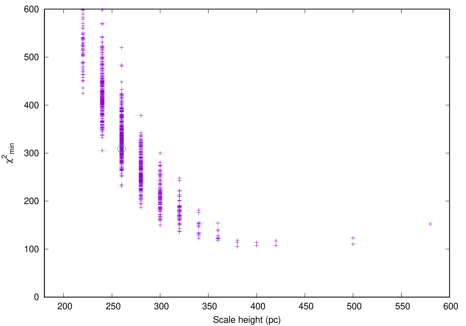
Figure 5: Minima of $\chi^{2}$ and scale heights that give the minima for 1000 realizations of LLFs. The number density for each magnitude bin of each random LLF is generated as a Gaussian random variable with the mean and standard deviation of the Cruz et al. LLF (CRUZ7). The mean LLF of Cruz et al. corresponds to the open circle at ($h$,$\chi^{2}_{min}$) = (260 pc, 309). The smallest $\chi^{2}$ is located at ($h$,$\chi^{2}_{min}$) = (380 pc, 106). The figure of merit $Q=3.0\times 10^{-15}$, which is significantly better than the mean Cruz model.

As expected, the number density of data points is largest around the data point for the MCRUZ model $(h,\chi^{2}_{min})=(260,309)$. However, there is an interesting trend that $\chi^{2}_{min}$s are smaller for larger $h$ and the smallest $\chi^{2}_{min}$ is located at $(h,\chi^{2}_{min})=$(380pc,106) with $Q(37|106)=3.0\times 10^{-15}$. The $\chi^{2}_{min}$ appears to increase beyond $h>400$ pc, but data points are so sparse and nothing definite can be said about where the true global minimum is. To investigate the reality of this apparent minimum, we form a LLF from the LLFs with the three lowest $\chi^{2}_{min}$ near $h=380$ pc, which we call ITERA (Table 4), meaning iteration. We use the LLF, ITERA as the seed LLF with the mean and standard deviation for the $\chi^{2}$ fitting and study the stability of the global minimum of $\chi^{2}_{min}$ found around $h=380$ pc. We generated another 1000 realizations of LLFs and calculated $\chi^{2}$ for $h$ from 200 to 580 pc with a 20 pc step and searched for the optimal $h$ and $\chi^{2}_{min}$. The resultant combinations of $h$ and $\chi^{2}_{min}$ are plotted in Figure 6. There is a global minimum of $\chi^{2}_{min}(global)$ of 103 at $h\sim 380$ pc, which gives the figure of merit, $Q(37|103)=2.2\times 10^{-14}$, which is slightly better than the result for ITERA. This iteration confirms that the global minimum found at $h=380$ is stable and the search for the solution converged. The final LLF, FINAL, was formed by averaging LLFs corresponding to the three lowest $\chi^{2}$s, and is given in Table 4.

This global minimum is rather broad as we can see from the following discussion of statistics. $\Delta\chi^{2}=\chi^{2}_{min}-\chi^{2}_{min}(global)$ follows the $\chi^{2}$ distribution of eight degrees of freedom (DOF= the number of free parameters to vary) (Lampton et al., 1976). The $\Delta\chi^{2}$ for a 90% confidence level is 12. The horizontal line drawn in Figure 6, shows this level and the data points below this line are within the 90% confidence interval. From the behavior of the lower envelope of data points in Figure 6, we can read that the 90% confidence interval is between 320 and 520 pc. This also implies that the MCRUZ model is ruled out with a very high confidence. This horizontal line for the 90% confidence level should be regarded as an upper bound, because of the following reason. We have assumed that the densities in individual magnitude bins are independent Gaussian random variables. However we know that there is a significant error in the absolute magnitude in each magnitude bin and neighboring bins are correlated. So effective degrees of freedom of free parameters should be less than eight although there is no clue at present to calculate this effective DOF. The lower DOF implies that the confidence level in Figure 6 should be lower and the confidence interval should be narrower. The model predictions by the mean number densities of FINAL and the observed L dwarf count are compared in Figure 7. We consider that the fit of the observed count with the model predictions is satisfactory.

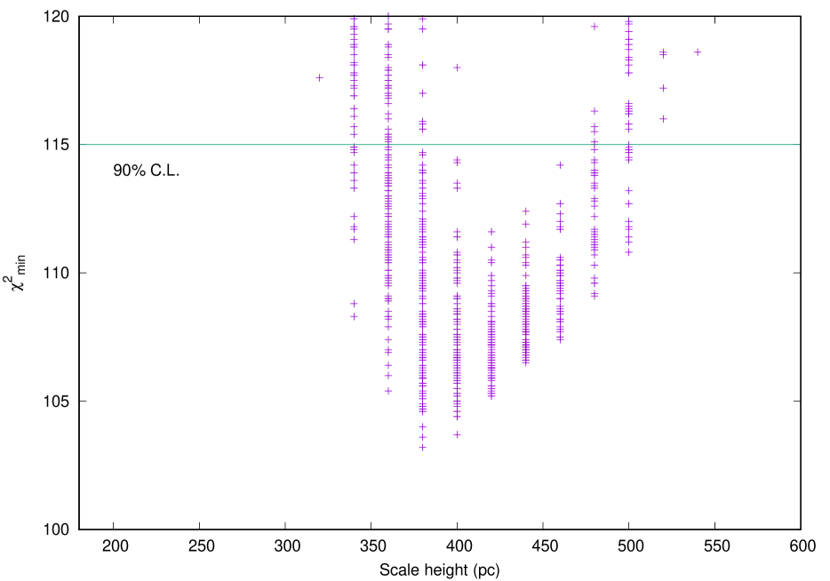
Figure 6: Minima of $\chi^{2}$ and scale heights for the ITERA model as input. The global minimum is found at ($h$, $\chi^{2}_{min}$) = (380 pc, 103), which is only slightly better than the input model result. This confirms the stability of the solution. $\Delta\chi^{2}=\chi^{2}_{min}-\chi^{2}_{min}(global)$ behaves as the $\chi^{2}$-distribution with DOF=8 (the number of free parameters). The 90% confidence level is shown as the green horizontal line, which indicates that the 90% confidence interval is between 320 and 520 pc.

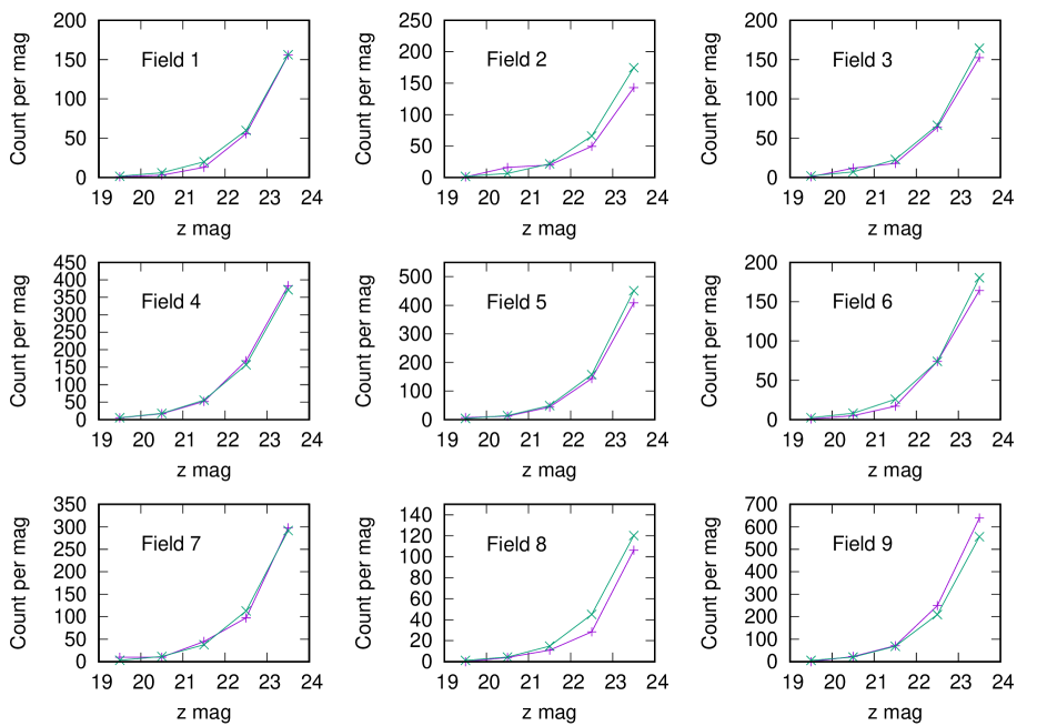
Figure 7: Comparison of observed counts (violet) and predictions by the FINAL model (green). The optimal $h=380$ pc and $\chi^{2}=103$ for DOF = 37. The figure of merit $Q=2.2\times 10^{-14}$, which is significantly larger than that for the MCRUZ model.

3.5 Comparison of three models

Here the three LLFs, MCRUZ, ITERA and FINAL are compared. These LLFs are numerically given in Table 4, and plotted in Figure 8.

The most striking feature in Figure 8 is that the brightest magnitude bin in MCRUZ ($M_{J}=11.75$) is greater than those of ITERA and FINAL by a factor of four. From the comparison between the observed count and prediction by the MCRUZ model in Figure 4, we notice that the MCRUZ model predicts excessive counts compared to observations in many fields. Those bright sources seen in MCRUZ do not exist in the observed count. The small scale height $h=260$ pc derived for this model appears to compensate for this excess at large distances from the Sun. One reason is conceivable for this behavior. The brightest bin corresponds to the bluest sources especially in $z-y$ in our sample, while the sample of Cruz et al. was selected by spectral type. So it is conceivable that the source counts near the M/L border ($M_{J}=11.75$) may to some extent disagree due to the difference in the source selection methods.

The second striking feature is that apart from the brightest magnitude bins, the three models agree reasonably well within the uncertainties of number densities of individual magnitude bins. This is rather surprising considering that the ITERA and FINAL models are results of the Monte Carlo method. Except for the brightest magnitude bins of ITERA and FINAL, MCRUZ was effectively unchanged. This indicates that the potential idiosyncrasy of the LLF of the Cruz et al. in the immediate solar neighborhood is small, even if it existed, except for the mystery of the brightest magnitude bin.

Figure 8: Comparison of LLFs, CRUZ7 (violet), ITERA (green) and FINAL (blue). The brightest magnitude bin in CRUZ7 is much greater than those of ITERA and FINAL. Apart from this brightest magnitude bin, three luminosity functions are not significantly different. Error bars are for 1-sigma errors.

3.6 Hybrid model

From the behavior of LLFs in the previous subsection, we can conjecture that the brightest magnitude bin is solely responsible for the major behavior of $\chi^{2}$ and the choice of LLF concerning the other magnitude bins is rather irrelevant. To investigate this possibility, we have fixed the magnitude bins other than the brightest one to those of MCRUZ, and performed $\chi^{2}$ fitting using the scale height and the density of the brightest magnitude bin as the only two free parameters. Since the parameter space is rather small, we need not to use the Monte Carlo technique. For the density of the brightest magnitude bin, we calculated 150 data points between $1.0\times 10^{-5}$ and $1.5\times 10^{-3}$ (pc^-3) in $1.0\times 10^{-5}$ step and generated 150 LLFs. $\chi^{2}$s were calculated for $h$ between 200 and 580 pc in a 20 pc step (3000 models), and $h$, which minimizes the $\chi^{2}$, was searched for for each LLF.

The result confirms our anticipation. The global minimum of $\chi^{2}$, was found at $(h,\chi^{2}_{min})=$(380 pc, 102), which is exactly the same as for the global minimum found for the Monte Carlo technique. We call this model, the HYBRD model (hybrid model), since the LLF for this model is partly MCRUZ and partly a random LLF. The number density for the brightest magnitude bin of HYBRD is $2.4\times 10^{-4}$ pc^-3. The figure of merit is $Q(43|102)=1.4\times 10^{-11}$, which is greater than that for the global minimum of the random LLF. The behavior of $\chi^{2}_{min}$ is plotted in Figure 9. Although the location of the minimum is the same, the width of the minimum is much narrower than the case of the fully random LLF. This is because we did not vary the lower six magnitude bins. $\Delta\chi^{2}=\chi^{2}_{min}-\chi^{2}_{min}(global)$ follows $\chi^{2}$ probability distribution of only two degrees of freedom. A 90% confidence interval is between 340 and 420 pc, while a 99% confidence interval is between 340 and 440 pc. This indicates that the vertical scale height for the global minimum, 380 pc, is rather secure.

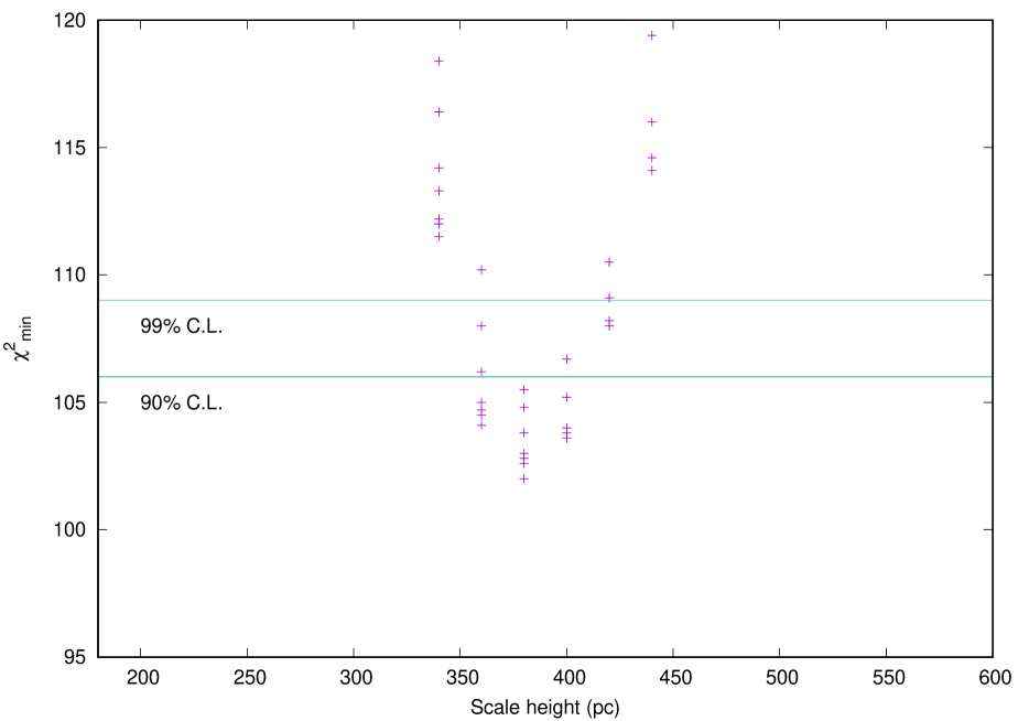
Figure 9: The global minimum (the HYBRD model) is found at ($h$, $\chi^{2}_{min}$) = (380 pc, 102), which is exactly the same for FINAL. $\Delta\chi^{2}=\chi^{2}_{min}-\chi^{2}_{min}(global)$ behaves as the $\chi^{2}$-distribution with DOF=2. The 90% and 99% confidence levels are shown as the green horizontal lines.

3.7 Effect of binaries

Here we try to evaluate the upper bound of the influence of binaries on our analysis. By NICMOS/HST imaging, Reid et al. (2008) obtained a binary fraction of L dwarfs within 20 pc to be $12.5^{+5.3}_{-3.0}$% after correcting for Malmquist bias. Taking into account the fact that there may be some binaries spatially unresolved even by HST, we here assume a binary fraction of 20% as an upper bound. Equal flux binaries have the maximum effect on the source count and we assume that all binaries are equal flux binaries. From the original source catalog, we generate a new catalog by assuming that each source is an equal flux binary with a 20% probability. We generate multiple new catalogs and average them to make a catalog containing binaries. The usual $\chi^{2}$ fitting is performed for the catalog containing binaries. The global minimum of $\chi^{2}_{min}=105$ is found at $h\sim 380$ pc. The LLF for this global minimum coincides with FINAL within errors. It turned out that the effect of binaries is smaller than that of the completeness correction mentioned above.

	MCRUZ	ITERA	FINAL	HYBRD
$h$(pc)	260	380	380	380
DOF	44	37	37	43
$\chi^{2}_{min}$	309	106	103	102
$Q$	$1.4\times 10^{-80}$	$3.0\times 10^{-15}$	$2.2\times 10^{-14}$	$1.4\times 10^{-11}$

Table 5: Results of fitting. The best-fit models are compared. MCRUZ stands for the model for the mean LLF of Cruz et al.(2007). ITERA is the result after varying the Cruz LLF (CRUZ7). FINAL is the result of the confirmation run using the ITERA model as input. HYBRD is the LLF with varying the brightest magnitude bin and static other bins fixed to those of MCRUZ. $h$ is the optimal scale height. DOF is the degrees of freedom of fitting. $Q$ is the figure of merit for fitting to compare the goodness of fit for different degrees of freedom. Larger the $Q$, better the fit.

4 Discussion

4.1 Comparison with previous works on brown dwarfs

As we have shown in Figure 1 (Comparison of ground-based surveys), previous ground-based wide-field surveys have not been able to detect L dwarfs at 300 pc. Therefore there has not been any attempt to estimate the vertical scale height based on the ground-based data. HST observations are deep enough to reach brown dwarfs well beyond 300 pc, but suffer from the small field of view and therefore from small number statistics. Estimates of the brown dwarf scale height are summarized in Table 6.

Based on 18 M and later dwarfs, Pirzkal et al. (2005) determined the vertical scale height of M and L dwarfs to be 400 $\pm$ 100 pc. For the purpose of comparing observations with Galaxy models they used model luminosity functions derived from Monte Carlo mass function simulations developed by Burgasser (2004) .

From 28 L and T dwarfs selected by $i^{\prime}-z^{\prime}$ color and morphology, Ryan et al. (2005) estimated the scale height of L and T dwarfs to be 350 $\pm$ 50 pc. In their analysis, L and T dwarfs were treated as a single population and a local number density for L and T dwarfs derived by Chabrier (2002) was used.

By infrared imaging, Ryan et al. (2011) discovered 17 ultracool dwarfs later than $\sim$M8 and estimated the vertical scale height to be 290 $\pm$ 25 (random) $\pm$ 31 (systematic). It should be noted that they used the LLFs of Cruz et al. (2007) for M8-L8 dwarfs and of Reylé et al. (2010) for T dwarfs. They took the uncertainties in the LLFs into account as we have done in the previous section and computed the systematic error. It is surprising that errors in the scale height are so small despite the small sample size of 17 sources. We suspect that the treatment of statistics in estimating the error due to uncertainties in the LLFs may not be appropriate. When individual magnitude bins in the LLFs are varied along with the scale height, there are more than ten DOF in $\Delta\chi^{2}=\chi^{2}-\chi^{2}_{min}$ distribution. This large dimension in the parameter space may result in a greater statistical error. Although there is some question in the error estimate, the work by Ryan et al. (2011) should be compared with ours from the point of view of the level of sophistication in analysis. Their result in $h=290$ pc is significantly smaller than our scale height estimate.

Table 6: Scale height estimates of brown dwarfs

Authors	Facility	Scale height
		pc	Comment
Pirzkal et al. (2005)	HST	400 $\pm$ 100	Simulated LF
Ryan et al. (2005)	HST	350 $\pm$ 50	L & T dwarfs treated as a single population
Ryan et al. (2011)	HST	290 $\pm$ 25(random) $\pm$ 31 (systematic)
This work(FINAL)	HSC	380${}^{+140}_{-60}$	90% confidence interval
This work(HYBRD)	HSC	380$\pm$ 40	90% confidence interval

Table 7: Scale height estimates of low mass stars

Authors	Facility	Scale height	Comment
		pc
Chen et al. (2001)	SDSS	330 $\pm$ 3	Fixed LF
Jurić et al. (2008)	SDSS	300 $\pm$ 60
Bochanski et al. (2010)	SDSS	300 $\pm$ 15
Pirzkal et al. (2009)	HST	370${}^{+60}_{-65}$	M4-M9 dwarfs
Pirzkal et al. (2009)	HST	300 $\pm$ 70	M0-M9 dwarfs
van Vledder et al. (2016)	HST	290${}^{+20}_{-19}$

4.2 Comparison with scale height estimates of low mass stars

To compare with the brown dwarf scale height, scale height estimates of low mass stars are summarized in Table 7. The most recent determinations of the vertical scale height of low mass stars are based on the SDSS data (Chen et al., 2001; Jurić et al., 2008; Bochanski et al., 2010). Chen et al. used the LLF of Wielen et al. (1983) and derived a thin-disk scale height of $h=330\pm 3$ pc for late-type dwarfs. Their error is so small because they adopted a fixed LLF. Jurić et al. used the photometric parallax method to estimate the distances to stars and mapped their three-dimensional number density distribution in the Galaxy. From Mote Carlo simulations, they estimated the errors of $\sim$20% in the disk scales and $\sim$10% in the density normalization. They derived a M dwarf scale height of $h=300\pm 60$ pc. They consider that the largest contributions to error come from the uncertainty in calibration of the photometric parallax relation and poorly constrained binary fraction. Bochanski et al. simultaneously measured Galactic structure and the stellar LF for stars with masses between 0.1 and 0.8M_⊙. They derived a thin disk scale height of $h=300\pm 15$ pc. Despite using somewhat different approaches, Jurić et al. and Bochanski et al. derived the same mean value of $h=300$ pc, which appears to represent the results from SDSS for low mass stars.

The estimation of the vertical scale height of M dwarfs has also been attempted by the use of the HST data (Pirzkal et al., 2009; van Vledder et al., 2016). Based on the sources selected from the ACS grism spectra, Pirzkal et al. estimated the vertical scale height of $h=370^{+60}_{-65}$ pc for M4-M9 dwarfs. They also derived the scale height for M0-M9 dwarfs to be $h=300\pm 70$ pc. In their analysis, they adopted the $z$-band LF of Bochanski et al. (2010) and the $J$-band LF of Cruz et al. (2007). van Vledder et al. selected 274 identified M dwarfs in the WFPC3 pure parallel fields from the BoRG survey for high-redshift galaxies. Although they use the terminology “M-type brown dwarfs”, what they mean by that appears to be ordinary M dwarfs. They derived the disk scale height of $h=290^{+20}_{-19}$ pc. As the scale height of M dwarfs (M0-M9), the results from the HST data also have a mean of the scale height around $h\sim 300$ pc, which is in accord with the results from the SDSS data.

The scale height of L dwarfs we derived from the HSC data (especially the HYBRD model) appears higher than the mean value for M dwarfs.

4.3 Comparison with kinematics of nearby dwarfs

One way to study the structure of the Galaxy is to investigate the kinematics of low mass stars and substellar objects in the immediate solar neighborhood. A study of tangential velocities for a large sample of late-type M, L, and T dwarfs has found that the kinematics of the sample show no significant differences between late-type M, L, and T dwarfs (Faherty et al., 2009). A recent study of $UVW$ velocities of late M dwarfs and L dwarfs shows interesting and mysterious results (Burgasser et al., 2015). While the simulations based on evolutionary models predict younger ages for L dwarfs than for M dwarfs, observations indicate older ages for L dwarfs (6.5 $\pm$ 0.4 Gyr) than for M dwarfs (4.0 $\pm$ 0.2 Gyr). The scale height we derived is qualitatively in accord with the results by Burgasser et al., since the scale height for L dwarfs (380 pc) appears to be larger than that for M dwarfs (300 pc).

5 Concluding remarks

We have analyzed DR1 of the HSC-SSP data aiming at determining the vertical scale height of L dwarfs in the Galactic thin disk, assuming an exponential disk model. We first used the mean LLF of Cruz et al. (2007), but this LLF resulted in a poor fit to the data even for an optimal scale height of $h=260$ pc. We then allowed the number densities for individual seven magnitude bins to vary along with the scale height, which is an eight parameter fit. We reached a reasonable fit for a scale height of $h=380$ pc. However, this minimum is broad and a 90 % confidence interval is between 320 and 520 pc. Then we restricted the free parameters to the scale height and the density of the brightest magnitude bin in the LLF, which is a two parameter fit. We reached an equally good fit to the eight parameter fit with the two parameter fit and a 90% confidence interval was between 340 and 420 pc. A deeper limiting magnitude is necessary to study the scale height of T dwarfs. The HSC ultra-deep survey will reach 1.7 magnitude deeper than the wide survey, although the survey area is 3.5 deg². We plan to pursue the possibility of utilizing this survey aiming at estimating the T dwarf scale height.

Appendix A Explicit treatment of the Malmquist bias

Here we treat the case of one particular stellar population, whose volume number density of the solar neighborhood is $n_{0}$, whose mean absolute magnitude is $M_{0}$ and its dispersion is $\sigma$. We follow the notation of the original work by Malmquist (1922).

If we denote by $a(m)$ the frequency function of the apparent magnitude $m$, then $a(m)dm$ is the number of stars having an apparent magnitude $m\pm dm/2$ and

$$\int_{m-1/2}^{m+1/2}dma(m)=N(m),$$ (A1)

is the differential number count at the apparent magnitude $m$ in units of the number per mag. If the relative frequency function of the absolute magnitude, $\varphi(M)$ has a Gaussian form as assumed by Malmquist,

$$\varphi(M)=\frac{1}{\sqrt{2\pi\sigma^{2}}}\exp\left(-\frac{(M-M_{0})^{2}}{2\sigma^{2}}\right),$$ (A2)

where $\int dM\varphi(M)=1$, and the volume number density at distance $r$ from us is $D(r)$, $a(m)$ is given by

$$a(m)=\omega\int_{0}^{+\infty}drr^{2}D(r)\varphi(M),$$ (A3)

and the differential number count is

$$N(m)=\omega\int_{m-1/2}^{m+1/2}dm\int_{0}^{+\infty}drr^{2}D(r)\varphi(M),$$ (A4)

where $\omega$ is the solid angle of the area of concern. In our exponential disk model,

$$D(r)\varphi(M)=n_{0}\exp\left(\frac{R_{0}-R}{H}-\frac{|Z|}{h}\right)\frac{1}{\sqrt{2\pi\sigma^{2}}}\exp\left(-\frac{(M-M_{0})^{2}}{2\sigma^{2}}\right),$$ (A5)

and

$$R(r,b,l) = \sqrt{R_{0}^{2}+(r\cos b)^{2}-2R_{0}r\cos b\cos l},$$ (A6)

$$Z(r,b) = Z_{\odot}+r\sin(b-\tan^{-1}(Z_{\odot}/R_{0})),$$ (A7)

$$M(m,r) = m-5\log r+5,$$ (A8)

where $Z_{\odot}$ is the height of the Sun from the Galactic plane. The effect of the Malmquist bias is explicitly taken into account by the numerical integration in the apparent magnitude $m$.

References

- Aihara et al. (2018) Aihara, H., Armstrong, R., Bickerton, S., et al. 2018, PASJ, 70, 8
- Arnaboldi et al. (2007) Arnaboldi, M., Neeser, M. J., Parker, L. C., et al. 2007, Msngr, 127, 28
- Barbaro & Olivi (1989) Barbaro, G. & Olivi, F., 1989, ApJ, 337, 125
- Bochanski et al. (2010) Bochanski, J. J., Hawley, S. L., Covey, K. R., et al. 2010, AJ, 139, 2679
- Burgasser (2004) Burgasser, A. J. 2004, ApJS, 155, 191
- Burgasser et al. (2015) Burgasser, A. J., Logsdon, S. E., Gagné, J., et al. 2015, ApJS, 220, 18
- Burningham et al. (2013) Burningham, B., Cardoso, C. V., Smith, L., et al. 2013, MNRAS, 433, 457
- Chabrier (2002) Chabrier, G. 2002, ApJ, 567, 304
- Chen et al. (2001) Chen, B., Stoughton, C., Smith, J. A., et al. 2001, ApJ, 553, 184
- Cruz et al. (2007) Cruz, K. L., Reid, I. N., Kirkpatrick, J. D., et al. 2007, AJ, 133, 439
- Day-Jones et al. (2013) Day-Jones, A. C., Marocco, F., Pinfield, D. J., et al. 2013, MNRAS, 430, 1171
- Delorme et al. (2010) Delorme, P., Albert, L., Forveille, T., et al. 2010, A&A, 518, 39
- Faherty et al. (2009) Faherty, J. K., Burgasser, A. J., Cruz, K. L., et al. 2009, AJ, 137, 1
- Filippazzo et al. (2015) Filippazzo, J. C., Rice, E. L., Faherty, J., et al. 2015, ApJ, 810, 158
- Jurić et al. (2008) Jurić, M., Ivezić, Z̆., Brooks, A., et al. 2008, ApJ, 673, 864
- Kirkpatrick et al. (2011) Kirkpatrick, J. D., Cushing, M. C., Gelino, C. R., et al. 2011, ApJS, 197, 19
- Kirkpatrick et al. (2012) Kirkpatrick, J. D., Gelino, C. R., Cushing, M. C., et al. 2012, ApJ, 753, 156
- Kirkpatrick et al. (2014) Kirkpatrick, J. D., Schneider, A., Fajardo-Acosta, S., et al. 2014, ApJ, 783, 122
- Lampton et al. (1976) Lampton, M., Margon, B. and Bowyer, S. 1976, ApJ, 208, 177
- Lawrence et al. (2007) Lawrence, A., Warren, S. J., Almaini, O., et al. 2007, MNRAS, 379, 1599
- Lépine & Scholz (2008) Lépine, S. and Scholz, R.-D. 2008, ApJ, 681, 33
- Lodieu et al. (2017) Lodieu, N., Espinoza Contreras, M., Zapatero Osorio, M. R. et al. 2017, A&A, 598, A92
- Malmquist (1922) Malmquist, K. G. 1922, Medd. Lunds. Obs. Ser I, 100
- Marocco et al. (2015) Marocco, F., Jones, H. R. A., Day-Jones, A. C., et al. 2015, MNRAS, 449, 3651
- Matsuoka et al. (2016) Matsuoka, Y., Onoue, M., Kashikawa, N., et al. 2016, ApJ, 828, 26
- Matsuoka et al. (2018a) Matsuoka, Y., Onoue, M., Kashikawa, N., et al. 2018, PASJ, 70, 35
- Matsuoka et al. (2018b) Matsuoka, Y., Iwasawa, K., Onoue, M. et al. 2018, ApJS, 237, 5
- Metchev et al. (2008) Metchev, S. A., Kirkpatrick, J. D., Berriman, G. B., & Looper, D. 2008, ApJ, 676, 1281
- Miyazaki et al. (2018) Miyazaki, S., Komiyama, Y., Kawanomoto, S. 2018, PASJ, 70, 1
- Pirzkal et al. (2005) Pirzkal, N., Sahu, K. C., Burgasser, A., et al. 2005, ApJ, 622, 319
- Pirzkal et al. (2009) Pirzkal, N., Burgasser, A. J., Malhotra, S., et al. 2009, ApJ, 695, 1591
- Reid et al. (2008) Reid, I. N., Cruz, K. L., Burgasser, A. J. & Liu, M. C. 2008, AJ, 135, 580
- Reylé et al. (2010) Reylé, C., Delorme, P., Willott, C. J., et al. 2010, A&A, 522, A112
- Ryan et al. (2005) Ryan, R. E., Hathi, N. P., Cohen, S. H., & Windhorst, R. A. 2005, ApJ, 631, L159
- Ryan et al. (2011) Ryan, R. E., Thorman, P. A., Yan, H., et al. 2011, ApJ, 739, 83
- Schlafly & Finkbeiner (2011) Schlafly, E. F. & Finkbeiner, D. P. 2011, ApJ, 737, 103
- Skrutskie et al. (2006) Skrutskie, M. F., Cutri, R. M., Stiening, R., et al. 2006, AJ, 131, 1163
- van Vledder et al. (2016) van Vledder, I., van der Vlugt, D., Holwerda, B. W., et al. 2016, MNRAS, 458, 425
- Wielen et al. (1983) Wielen, R., Jahreiß, H. & Krüger, R. 1983, in IAU Colloq. 76: Nearby Stars and the Stellar Luminosity Function, ed. Philip, A. G. D. & Upgren, A. R.,
- Wright et al. (2010) Wright, E. L., Eisenhardt, P. R. M., Mainzer, A. K. et al. 2010, AJ, 140, 1868
- Yamada et al. (2005) Yamada, T., Kodama, T., Akiyama, M., et al. 2005, ApJ, 634, 861
- York et al. (2000) York, D. G., Adelman, J., Anderson, Jr., J. E., et al. 2000, AJ, 120, 1579