Basic observables for the accelerated electron and its field

Abstract

We revisit in the framework of the classical theory the problem of the accelerated motion of an electron, taking into account the effect of the radiation emission. We present results for the momentum and energy of the electromagnetic field of an accelerated electron for a spatial region excluding a vicinity of the electron and a procedure to compensate their singularities in the limit of the point electron. From them we infer expressions for the observables momentum and energy of the electron. They lead, together with those corresponding to the emitted radiation, to an equation of motion of the electron that coincides, in the case of an external electromagnetic field, with the Lorentz-Dirac equation. Based on the results for the linear momentum and using the same calculation method, we obtain the equations corresponding to the angular momentum of the electron and its field. While the formalism used is not wholly manifestly covariant, arguments based on relativistic covariance are invoked and used at appropriate places, where they play an essential role.

I Introduction

The collision processes of high energy electrons with other charged particles or with intense laser pulses can be strongly influenced by the emission of radiation accompanying these processes. The experimental observation of this influence or reaction, usually called radiation reaction (RR), in the case of electrons colliding with laser pulses, as well as of other strong fields effects and processes, became possible nowadays due to the remarkable progresses registered by the laser technology – see adpk for a recent review of high-energy processes in extremely intense laser fields. Two very recent papers poder ; cole present and analyze experimental results proving for the first time a strong radiation reaction regime in the interaction of relativistic electrons with ultra-high intensity laser pulses. They illustrate the actual limitations for observing RR and the inherent difficulties to validate the theoretical models for RR. While non-negligible quantum effects are predicted for conditions of the quoted experiments, the data obtained seem to not allow a clear discrimination between classical and quantum models – see also the viewpoint expressed in macchi .

The above mentioned actual context and the future experiments planned for higher intensities of laser pulses at other laser facilities (as, for example, at ELI-NP turcu ) indicate the need for a better description of RR, in both classical and quantum theory. In particular, one may appreciate that a progress in the classical theory of RR (the only one considered in this paper) in understanding the basic observables of the electron and its field, would lead to a more consistent description of the reaction effect. This potential progress should be also beneficial for the formulation of a more accurate quantum description of RR and for an improved understanding of the quantum-classical correspondence relation.

We recall that the description of the accelerated motion of an electron with the inclusion of RR – see hammond ; burt for qualified introductions on the subject, discussions of the main equations used for RR and for the relevant references – presents considerable difficulties (no matters the cause of acceleration, the presence of an external field or the interaction with other particles), related to the treatment of the electromagnetic field of the moving electron - the evolution of this field depends on the motion of the electron and, in turn, influences this motion. Rather interesting and somehow unexpected, the problem of finding the reaction of the electromagnetic field on the motion of an electron accelerated by an external field admits a closed solution (recalled below). Most frequently, the approaches used to solve this problem concentrate on the forces which determine the motion of the electron. Besides the external force acting on the electron one has to take into account the apparent force related to the momentum transported by the electromagnetic field of the moving electron. This reaction force is called radiation reaction force or radiation damping (or friction) force, terminology used even if one cannot fully explain the origin of the reaction on the base of the emitted radiation. In fact, two types of electromagnetic reaction forces can be identified, one of them is directly connected with the radiation and vanishes in the non-relativistic limit, the other being in the same limit proportional to the time derivative of the electron acceleration and being termed sometimes Abraham (or Abraham-Lorentz) force or self-force.

The existing calculations of the electromagnetic reactions consider the electron either as an extended charged particle of finite size with a corresponding charge distribution (the Lorentz model) or as a point charge. The Lorentz model of the electron was fully abandoned in dirac , where a formalism based on retarded and advanced potentials was build for a point charged particle, culminating with the derivation of the equation of motion of the electron. This equation coincides with that emerging approximately from the Lorentz model and it is usually termed Lorentz-Abraham-Dirac (LAD) or simply Lorentz-Dirac equation. The problem of the uniqueness of the motion equation was analyzed in bhabha and it was shown that for a point particle in electromagnetic field the conservation of the angular momentum, not implied in general by this equation, has to be imposed distinctly. This leads to supplementary constraints on the form of the equation, which is unique and coincides with LAD equation if one requires also to not contain derivatives of the electron velocity of an order higher than the second one. Another derivation of LAD equation, based on a decomposition of the Maxwell tensor and not relying on the advanced fields, was presented in titbo .

The issue related to the order of LAD equation (third order with respect to time) and its unphysical consequences is overcome if in place of it one works with Landau-Lifshitz (LL) equation ll . This second order equation, being an approximation of LAD equation, was questioned about its validity range, investigation presenting an increasing interest for the actual context. Alternative theories to LAD and LL equations where described in the literature – see burt and references therein. We mention here Ref. soko , which attracted some interest in the last years, in particular for the possibility to regard the relation of the velocity and the momentum of the electron as being a Lorentz transformation induced by the external electromagnetic field capdes . The set of equations proposed in soko , replacing approximately LAD equation, and equivalent with LL equation but numerically simpler capdes , is based on the idea that the 4-vectors velocity and momentum of an accelerated electron might be introduced such they are not-collinear, and on supplementary assumptions, in particular that of the validity of the momentum-energy Einstein relation.

The approach employed in this paper to investigate the electromagnetic reaction is based on the examination of the fundamental observables of the compound system (electron and electromagnetic field), followed then by the analysis of their implications. In place of directly targeting the equations of motion, we focus on the problem of finding the expressions of the momentum, energy and angular momentum of an electron accelerated by an external force. We adhere to the assumptions of dirac - the electron is a point charged particle, the Maxwell equations are supposed valid everywhere and, consequently, the fields are singular at the electron position. In Sect. II we first describe the results obtained for the momentum and energy of the electromagnetic field of an accelerated electron. The method we use to calculate them, presented in Appendix, allows to clearly separate the terms corresponding to the emitted radiation from those bound to the electron. In order to treat the singularities (associated with the zero size of the electron) of the latter terms and their partial covariance, we adopt a simple compensation procedure then we infer the expressions of the electron observables, analyze their main features and follow some implications. From the formulas for the momentum and energy of the electron and its electromagnetic field we simply re-derive the electromagnetic reaction forces and formulate the equations of motion of the electron, finally re-obtaining the LAD equation.

In Sect. III we refer to another important observable, the angular momentum. The starting point is the angular momentum of the electromagnetic field of the accelerated electron. Its calculation is performed by the method used in Sect. II and is also described in Appendix. Adding to it the angular momentum of the bare electron, then considering the limit of the point electron we finally obtain the expression of the total angular momentum. In the last part of Sect. III we examine the balance of the angular momentum, the generalization of the corresponding theorem and some consequences of it.

II Momentum and energy

For the beginning it is convenient to review some basic relations of the relativistic kinematics for the case of an electron in arbitrary motion. We denote by ${\bf r}_{e}(t)$ the position of the electron as function of the time $t$ and by $x^{\mu}\equiv(ct,{\bf r}_{e})$ the corresponding 4-vector of the position. With ${\bf v}\equiv\dot{{\bf r}}_{e}\equiv d{\bf r}_{e}/dt$ the (usual) velocity of the electron, the Lorentz factor is

$$\gamma\equiv\frac{1}{\sqrt{1-{\mbox{\boldmath$\beta$}}^{2}}},\quad{\mbox{\boldmath$\beta$}}\equiv\frac{{\bf v}}{c}.$$ (1)

Differentiating successively the 4-position to $\tau$, the electron proper time, defined by

$$d\tau=\sqrt{1-{\mbox{\boldmath$\beta$}}^{2}}\,dt=\frac{dt}{\gamma},$$ (2)

one obtain the 4-vectors velocity $u^{\mu}\equiv(u^{0},{\bf u})$ and acceleration $a^{\mu}\equiv(a^{0},{\bf a})$. They are given by

$$u^{\mu}=\frac{dx^{\mu}}{d\tau}=(\gamma c,\gamma{\bf v})=c\,(\gamma,\gamma{\mbox{\boldmath$\beta$}})$$ (3)

and

$$a^{\mu}=\frac{du^{\mu}}{d\tau}=c\,\left(\gamma\,\frac{d\gamma}{dt},\gamma\,\frac{d}{dt}(\gamma{\mbox{\boldmath$\beta$}})\right)=c\,\gamma^{2}\,\left({\gamma}^{2}({\mbox{\boldmath$\beta$}}\cdot\dot{{\mbox{\boldmath$\beta$}}}),\dot{{\mbox{\boldmath$\beta$}}}+\gamma^{2}({\mbox{\boldmath$\beta$}}\cdot\dot{{\mbox{\boldmath$\beta$}}}){\mbox{\boldmath$\beta$}}\right).$$ (4)

The 4-scalar

$${\bf a}^{2}-(a^{0})^{2}={c^{2}}\gamma^{4}\left[{\dot{{\mbox{\boldmath$\beta$}}}}^{2}+\gamma^{2}({\mbox{\boldmath$\beta$}}\cdot\dot{{\mbox{\boldmath$\beta$}}})^{2}\right]=c\gamma^{2}\dot{{\mbox{\boldmath$\beta$}}}\cdot{\bf a}$$ (5)

presents a special interest in the following. Another relation implied by Eqs. (3) and (4),

$$a^{0}={\mbox{\boldmath$\beta$}}\cdot{\bf a},$$ (6)

equivalent to the orthogonality of 4-velocity and 4-acceleration, proves also to be useful.

We next recall that a free electron, moving with constant velocity ${\bf v}$, has a linear momentum ${\bf p}_{e}$ and a total energy $W_{e}$, given by

$${\bf p}_{e}=m\gamma{\bf v},\quad W_{e}=mc^{2}\gamma,$$ (7)

where $m$ is the electron mass. These quantities satisfy the well-known equation

$$W_{e}^{2}=m^{2}c^{4}+c^{2}{\bf p}_{e}^{2},$$ (8)

relating the particle energy to the magnitude of its linear momentum. The momentum and energy (divided by $c$) of the particle are the components of the 4-momentum

$$p_{e}^{\mu}=(W_{e}/c,{\bf p}_{e}),$$ (9)

proportional to the 4-velocity (3), $p_{e}^{\mu}=mu^{\mu}$.

We investigate in the following how the above relations for momentum and energy of a free electron are modified in the case of an electron moving in the field of an external force ${\bf F}$. These modifications are expected since, due to the fact that an accelerated electron emits electromagnetic radiation, its motion does not coincide with that of a neutral particle of the same mass which would be exposed to the same force ${\bf F}$.

For finding the relations replacing Eq. (7) in the case of an accelerated electron, we first take in consideration that the radiation emitted by the electron during its motion up to the actual time $t$, carries momentum and energy and denote these quantities by ${\bf p}_{rad}(t)$ and $W_{rad}(t)$. For the momentum and energy of the electron we use the same notations as in the case of the free electron, ${\bf p}_{e}(t)$ and $W_{e}(t)$ (they are now functions of time). If the electron was accelerated in the past but is free at the time $t$, i.e. $\dot{{\mbox{\boldmath$\beta$}}}(t)=0$, ${\bf p}_{e}(t)$ and $W_{e}(t)$ are again given by Eq. (7) and the total momentum ${\bf P}$ and the total energy $W$ of the compound system (electron and radiation) can be expressed as follows

$${\bf P}(t)={\bf p}_{e}(t)+{\bf p}_{rad}(t),\quad W(t)=W_{e}(t)+W_{rad}(t).$$ (10)

Two types of contributions shall be supposed below as being included in ${\bf p}_{e}(t)$ and $W_{e}(t)$, of the own field of the electron (field not-leaving the electron as radiation), and of the ”bare” electron, regarded as the other facet of the entity ”electron”. With further interpretation, these contributions, which combine to reproduce the results (7) in the case of the free electron, are such Eq. (10) is verified for the accelerated electron too (by definition, no contributions are included in $W_{e}$ corresponding to the interaction with the external field).

In order to reach the above announced objective we examine first the problem of the total momentum and energy of the electromagnetic field accompanying an accelerated electron. For their calculation we use the general expressions given by classical electrodynamics for the momentum density ${\bf g}$ and energy density $u$ of the field

$${\bf g}=\varepsilon_{0}\,{\bf E}\times{\bf B},\quad u=\frac{\varepsilon_{0}}{2}\left({\bf E}^{2}+c^{2}{\bf B}^{2}\right),$$ (11)

together with the expressions of the electric field ${\bf E}$ and magnetic field ${\bf B}$ generated by an electron in its motion, the so-called Liénard-Wiechert fields. At an observation point ${\bf r}$ and for the actual time moment $t$, these are given by jack

$${\bf E}({\bf r},t)=\frac{e}{4\pi\varepsilon_{0}}\frac{1-\beta^{2}}{R^{2}\varkappa^{3}}\,({\bf n}-{\mbox{\boldmath$\beta$}})+\frac{e}{4\pi\varepsilon_{0}c}\frac{1}{R\varkappa^{3}}\,{\bf n}\times\left[({\bf n}-{\mbox{\boldmath$\beta$}})\times\dot{{\mbox{\boldmath$\beta$}}}\right],\quad{\bf B}({\bf r},t)=\frac{1}{c}\,{\bf n}\times{\bf E}({\bf r},t),$$ (12)

where ${\bf n}$ is the unit vector along ${\bf R}\equiv{\bf r}-{\bf r}_{e}$ and $\varkappa\equiv 1-{\bf n}\cdot{\mbox{\boldmath$\beta$}}$. The expressions of the fields have to be evaluated at the retarded time moment $t^{\prime}$, verifying the equation

$$t^{\prime}=t-R(t^{\prime})/c,\quad R(t^{\prime})=|{\bf r}-{\bf r}_{e}(t^{\prime})|,$$ (13)

and uniquely determined by ${\bf r}$ and $t$ (for a given motion ${\bf r}_{e}(t)$ of the electron).

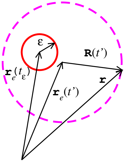
Figure 1: (Color online) The region $\cal D$ considered in the paper for integration is the exterior of the sphere (represented by the solid line circle) of radius ${\varepsilon}$. The vector ${\bf r}$ describes an arbitrary position in $\cal D$, while ${\bf r}_{e}(t^{\prime})$ is the electron position at the retarded time moment $t^{\prime}$ (anterior to $t_{{\varepsilon}}$), verifying Eq. (13).

Like the fields, the densities (11) are singular at ${\bf r}={\bf r}_{e}(t)$, the actual electron position. These singularities are not-integrable in general, the integration of the densities (11) over a region containing the singularity leading to infinite values for total momentum and total energy. This difficulty can be postponed calculating first the momentum and energy (at a given time $t$) of the field in a spatial region $\cal D$ taken to be the whole space minus a small region around the particle, then examining the limit where that small region reduces to the point ${\bf r}_{e}(t)$. The appropriate choice for ${\cal D}$ is that of a region outside a sphere of radius ${\varepsilon}$ (see Figure 1), centered on the position ${\bf r}_{e}(t_{{\varepsilon}})$ of the electron at the time moment $t_{{\varepsilon}}\equiv t-{{\varepsilon}}/c$. With this choice the spatial integration on $\cal D$ can be performed changing the integration variables from the coordinates ${\bf r}$ to the spherical coordinates of ${\bf R}(t^{\prime})={\bf r}-{\bf r}_{e}(t^{\prime})$. The calculation, presented in the Appendix, leads to the following results for the momentum

$${\bf G}({\varepsilon},t)=\frac{2}{3}\frac{e_{0}^{2}}{c}\frac{\gamma^{2}(t_{{\varepsilon}}){\mbox{\boldmath$\beta$}}(t_{{\varepsilon}})}{{\varepsilon}}+\frac{2}{3}\frac{e_{0}^{2}}{c^{2}}\int_{-\infty}^{t_{{\varepsilon}}}\gamma^{4}\left[{\dot{{\mbox{\boldmath$\beta$}}}}^{2}+\gamma^{2}({\mbox{\boldmath$\beta$}}\cdot\dot{{\mbox{\boldmath$\beta$}}})^{2}\right]{\mbox{\boldmath$\beta$}}\,dt^{\prime},$$ (14)

and for the energy

$$W({\varepsilon},t)=\frac{2}{3}\,{e_{0}^{2}}\frac{\gamma^{2}(t_{{\varepsilon}})-1/4}{{\varepsilon}}+\frac{2}{3}\frac{e_{0}^{2}}{c}\int_{-\infty}^{t_{{\varepsilon}}}\gamma^{4}\left[{\dot{{\mbox{\boldmath$\beta$}}}}^{2}+\gamma^{2}({\mbox{\boldmath$\beta$}}\cdot\dot{{\mbox{\boldmath$\beta$}}})^{2}\right]\,dt^{\prime}$$ (15)

of the electromagnetic field in $\cal D$, with the notation $e_{0}\equiv e/\sqrt{4\pi{\varepsilon}_{0}}$. The terms containing the integrals are the contributions of the acceleration fields, the others include velocity fields and mixed contributions (see the Appendix).

We examine the case where ${\cal D}$ covers the whole space, this meaning to look to the limit ${\varepsilon}\rightarrow 0$ ( $t_{{\varepsilon}}=t-{\varepsilon}/c\rightarrow t$) in Eqs. (14) and (15). The last terms in these equations do not raise problems when ${\varepsilon}\rightarrow 0$ and we identify them with the momentum

$${\bf p}_{rad}=\frac{2}{3}\frac{e_{0}^{2}}{c^{2}}\int_{-\infty}^{t}\gamma^{4}\left[{\dot{{\mbox{\boldmath$\beta$}}}}^{2}+\gamma^{2}({\mbox{\boldmath$\beta$}}\cdot\dot{{\mbox{\boldmath$\beta$}}})^{2}\right]{\mbox{\boldmath$\beta$}}\,dt^{\prime}$$ (16)

and the energy

$$W_{rad}=\frac{2}{3}\frac{e_{0}^{2}}{c}\int_{-\infty}^{t}\gamma^{4}\left[{\dot{{\mbox{\boldmath$\beta$}}}}^{2}+\gamma^{2}({\mbox{\boldmath$\beta$}}\cdot\dot{{\mbox{\boldmath$\beta$}}})^{2}\right]\,dt^{\prime}$$ (17)

of the radiation emitted up to the time $t$. The energy radiated by the electron per unit of time, $dW_{rad}/dt$, is the well-known Liénard-Larmor power

$${\cal P}_{L}=\frac{2}{3}\frac{e_{0}^{2}}{c}\,\gamma^{4}\left[{\dot{{\mbox{\boldmath$\beta$}}}}^{2}+\gamma^{2}({\mbox{\boldmath$\beta$}}\cdot\dot{{\mbox{\boldmath$\beta$}}})^{2}\right]=\frac{2}{3}\frac{e_{0}^{2}}{c^{3}}\gamma^{4}\left[\dot{{\bf v}}^{2}+\gamma^{2}({\mbox{\boldmath$\beta$}}\cdot\dot{{\bf v}})^{2}\right],$$ (18)

where $\dot{{\bf v}}=d{\bf v}/dt$ is the usual 3-vector acceleration. Being proportional to the 4-scalar (5), ${\cal P}_{L}$ is a 4-scalar in its turn. We remark that the rate of variation of ${\bf p}_{rad}$ (the time derivative $d{\bf p}_{rad}/dt$) has the direction of the electron velocity and is equal to the product of the mass radiated per time unit, ${\cal P}_{L}/c^{2}$, by the velocity ${\bf v}=c{\mbox{\boldmath$\beta$}}$ of the electron. The negative of this rate ($-d{\bf p}_{rad}/dt$) appears as a damping force due to radiation (see Eq. (52) from below). The quantities $W_{rad}/c$ and ${\bf p}_{rad}$ are the components of a 4-vector, the 4-momentum of the emitted radiation.

The other terms entering in Eqs. (14) and (15), denoted conveniently

$${{\bf p}}_{f}({\varepsilon},t)\equiv\frac{2}{3}\frac{e_{0}^{2}}{c}\frac{\gamma^{2}(t_{{\varepsilon}}){\mbox{\boldmath$\beta$}}(t_{{\varepsilon}})}{{\varepsilon}},$$ (19)

and

$$W_{f}({\varepsilon},t)\equiv\frac{2}{3}\,{e_{0}^{2}}\frac{\gamma^{2}(t_{{\varepsilon}})-1/4}{{\varepsilon}},$$ (20)

are, respectively, the momentum and the energy of the field (in the region $\cal D$) not leaving the electron as electromagnetic radiation. These terms are bound to the electron and we note that they are singular in the limit ${\varepsilon}\rightarrow 0$ in the general case. There is an exception, however, where the singularity does not manifest. This is related to the momentum of the field of an electron instantaneously at rest at the actual time $t$, e.g. ${\mbox{\boldmath$\beta$}}(t)=0$. For this case, replacing in Eq. (19) ${\mbox{\boldmath$\beta$}}(t_{{\varepsilon}})$ by its Taylor series expansion ${\mbox{\boldmath$\beta$}}(t_{{\varepsilon}})={\mbox{\boldmath$\beta$}}(t-{{\varepsilon}}/c)=-({{\varepsilon}}/c)\,\dot{{\mbox{\boldmath$\beta$}}}(t)+{\cal O}({\varepsilon}^{2})$, it follows that ${\bf p}_{f}({\varepsilon},t)$ has a finite limit for ${\varepsilon}\rightarrow 0$, proportional to the (usual) acceleration of the electron,

$${\bf p}_{f}(t)=-\frac{2}{3}\frac{e_{0}^{2}}{c^{2}}\,\dot{{\mbox{\boldmath$\beta$}}}(t)=-\frac{2}{3}\frac{e_{0}^{2}}{c^{3}}\,\dot{{\bf v}}(t).$$ (21)

Its negative rate of changing $(-d{\bf p}_{f}/dt)$ coincides with the non-relativistic Abraham force (self-force) [see below Eq. (51) for its relativistic generalization]. In the same limit the field energy can be approximated as $W_{f}({\varepsilon},t)\approx\frac{1}{2}\,{e_{0}^{2}}/{{\varepsilon}},$ and tends to infinity when ${{\varepsilon}}\rightarrow 0$.

In passing, for ${\bf v}(t)\neq 0$, we may note that in the non-relativistic theory, in the first order of ${\bf v}/c$ and for a fixed small ${\varepsilon}$, replacing $\gamma(t_{\varepsilon})=1$ in Eqs. (19) and (20) we can write ${{\bf p}}_{f}({\varepsilon},t)=m^{\prime}\,{\bf v}$ and $W_{f}({\varepsilon},t)=m^{\prime\prime}c^{2}$, where the masses $m^{\prime}$ and $m^{\prime\prime}$ depend on ${\varepsilon}$ and have the ratio $m^{\prime}/m^{\prime\prime}=4/3$ - this is a ”reincarnation” of the infame ”4/3” problem, first met in the case of an extended electron.

Returning to the general case, one sees that, besides the issue of singularities in the limit ${{\varepsilon}}\rightarrow 0$, Eqs. (19) and (20) display an improper relativistic behavior. This feature is not so surprising - as discussed in jack , integrating spatially the densities (11) for a general electromagnetic field, the resulting field energy (divided by $c$) and momentum form a 4-vector if the electromagnetic stress tensor is divergenceless, condition not fulfilled in the presence of the sources (our case). One way to remedy the covariance ”defect” is to modify the expressions of momentum and energy of the field – see, for example, Refs. titbo and jack . We don’t pursue this thread here since it seems not possible to sustain with convincing arguments that the own field momentum has to be a true observable. Another possibility, preferred in the following, is to admit that the ”bare” electron contributions are such to ”fix” both the singularity issue and the covariance property. While the nature of these contributions can’t be elucidated in the context of the present theory, we may assume that they are such to compensate the above mentioned singularities in the limit ${{\varepsilon}}\rightarrow 0$, at the same time leading to correct relativistic expressions for the total momentum and energy of the electron and reproducing in particular the relations (7) for the free electron case.

These considerations shall be applied below, after we analyze in detail Eqs. (19) and (20) around ${\varepsilon}=0$. Their structure becomes transparent if one replace the functions of $t_{{\varepsilon}}$ contained in these equations by their Taylor series expansions around the actual time $t$. One obtain the power series (in ${\varepsilon}$)

$${{\bf p}}_{f}({\varepsilon},t)\equiv\frac{2}{3}\frac{e_{0}^{2}}{c}\frac{\gamma^{2}{\mbox{\boldmath$\beta$}}}{{\varepsilon}}-\frac{2}{3}\frac{e_{0}^{2}}{c^{2}}\frac{d}{dt}(\gamma^{2}{\mbox{\boldmath$\beta$}})+{\cal O}({\varepsilon}),$$ (22)

and

$$W_{f}({\varepsilon},t)\equiv\frac{2}{3}\,{e_{0}^{2}}\frac{\gamma^{2}-1/4}{{\varepsilon}}-\frac{2}{3}\,\frac{e_{0}^{2}}{c}\frac{d}{dt}(\gamma^{2})+{\cal O}({\varepsilon})$$ (23)

(the time argument $t$ on the right side has been removed) - since we are interested about the limit ${\varepsilon}\rightarrow 0$, it is sufficient to analyze only the terms explicitly written.

The singular terms in the right hand side of Eqs. (22) and (23), of the order $1/{\varepsilon}$, coincide with the momentum and energy of the field in the case of a free electron that would have the velocity $c{\mbox{\boldmath$\beta$}}(t)$. The terms on the second position, finite and independent on ${\varepsilon}$, do not have (as also the first ones) proper relativistic behavior. We isolate from them a 4-vector whose spatial part reduces to the result (21) for ${\mbox{\boldmath$\beta$}}(t)\rightarrow 0$. Replacing first the derivative of $\gamma^{2}{\mbox{\boldmath$\beta$}}$ in Eq. (22) by the formula for the product $\gamma(\gamma{\mbox{\boldmath$\beta$}})$, one obtains the equivalent form

$${{\bf p}}_{f}({\varepsilon},t)\equiv\frac{2}{3}\frac{e_{0}^{2}}{c}\frac{\gamma^{2}{\mbox{\boldmath$\beta$}}}{{\varepsilon}}-\frac{2}{3}\frac{e_{0}^{2}}{c^{2}}\dot{\gamma}\,\gamma{\mbox{\boldmath$\beta$}}+{\bf p}_{S}+{\cal O}({\varepsilon}),$$ (24)

where the last term

$${\bf p}_{S}\equiv-\frac{2}{3}\frac{e_{0}^{2}}{c^{2}}\,\gamma\,\frac{d}{dt}(\gamma{\mbox{\boldmath$\beta$}})=-\frac{2}{3}\frac{e_{0}^{2}}{c^{3}}\,\gamma\,\frac{d}{dt}(\gamma{\bf v}),$$ (25)

is the spatial part of a 4-vector proportional to the 4-acceleration (4). The corresponding time component is

$$p_{S}^{0}=-\frac{2}{3}\frac{e_{0}^{2}}{c^{2}}\,\gamma\,\frac{d\gamma}{dt},$$ (26)

and one sees that the energy

$$W_{S}\equiv cp_{S}^{0}=-\frac{2}{3}\frac{e_{0}^{2}}{c}\,\dot{\gamma}\gamma$$ (27)

is one half of the last term in Eq. (23), so we can write

$$W_{f}({\varepsilon},t)\equiv\frac{2}{3}\,{e_{0}^{2}}\frac{\gamma^{2}-1/4}{{\varepsilon}}-\frac{2}{3}\,\frac{e_{0}^{2}}{c}\dot{\gamma}\,\gamma+W_{S}+{\cal O}({\varepsilon}).$$ (28)

We note a special feature of the relations (24) and (28): they describe quantities which depend solely on the state of the electron at the present time moment $t$, in contrast with ${\bf p}_{rad}$ and $W_{rad}$ from Eqs. (16) and (17), that depend on the whole past motion of the electron. If these quantities would be fully acceptable, this feature would enable us to regard them as characterizing the actual electron state. Since they are not, we are left with an indication that the problem has to be solved at the level of the electron itself. In this order we shift the attention to the other facet of the electron, the ”bare” electron, and consider its contributions to the momentum and energy of the electron, denoted, respectively, by $\overline{{\bf p}}_{e}({\varepsilon},t)$ and $\overline{W}_{e}({\varepsilon},t)$. For the total quantities of the electron we then have

$${{\bf p}}_{e}({\varepsilon},t)\equiv\overline{{\bf p}}_{e}({\varepsilon},t)+{\bf p}_{f}({\varepsilon},t),\quad{W}_{e}({\varepsilon},t)\equiv\overline{W}_{e}({\varepsilon},t)+W_{f}({\varepsilon},t),$$ (29)

and we build the power series for $\overline{{\bf p}}_{e}({\varepsilon},t)$ and $\overline{W}_{e}({\varepsilon},t)$ such to compensate both the singular and the non-covariant terms in Eqs. (24) and (28), and to lead to correct results for the free electron case. We infer that the power series in ${\varepsilon}$ for $\overline{{\bf p}}_{e}({\varepsilon},t)$ and $\overline{W}_{e}({\varepsilon},t)$ are, respectively,

$$\overline{{\bf p}}_{e}({\varepsilon},t)=-\frac{2}{3}\frac{e_{0}^{2}}{c}\frac{\gamma^{2}{\mbox{\boldmath$\beta$}}}{{\varepsilon}}+\frac{2}{3}\frac{e_{0}^{2}}{c^{2}}\dot{\gamma}\,\gamma{\mbox{\boldmath$\beta$}}+mc\gamma{\mbox{\boldmath$\beta$}}+{\cal O}({\varepsilon}),$$ (30)

and

$$\overline{W}_{e}({\varepsilon},t)=-\frac{2}{3}\,{e_{0}^{2}}\frac{\gamma^{2}-1/4}{{\varepsilon}}+\frac{2}{3}\,\frac{e_{0}^{2}}{c}\dot{\gamma}\,\gamma+mc^{2}\gamma+{\cal O}({\varepsilon}).$$ (31)

The terms on the first two positions in each equation are, up to the sign, the same as in Eqs. (24) and (28). On the last positions are included the momentum and energy of a free electron with velocity $c{\mbox{\boldmath$\beta$}}(t)$ - this guarantees the correctness of the equations for ${\bf p}_{e}$ and $W_{e}$ in the case the acceleration vanishes.

Passing to the limit ${{\varepsilon}}\rightarrow 0$ in Eqs. (29), we finally obtain the expressions for the electron momentum,

$${\bf p}_{e}=mc\gamma{\mbox{\boldmath$\beta$}}+{\bf p}_{S},$$ (32)

and its energy,

$$W_{e}=mc^{2}\gamma+W_{S}$$ (33)

(all the quantities are at the same time $t$). The last term in Eq. (33) is the so called Schott energy (or acceleration energy), $W_{S}=cp_{S}^{0}$. Using Eq. (26) and the rate $\dot{\gamma}=\gamma^{3}\,{\mbox{\boldmath$\beta$}}\cdot\dot{{\mbox{\boldmath$\beta$}}}$ of the Lorentz factor $\gamma$, it can be expressed as

$$W_{S}=-\frac{2}{3}\frac{e_{0}^{2}}{c}\,\gamma^{4}\,{\mbox{\boldmath$\beta$}}\cdot\dot{{\mbox{\boldmath$\beta$}}}=-\frac{2}{3}\frac{e_{0}^{2}}{c^{3}}\,\gamma^{4}\,{\bf v}\cdot\dot{{\bf v}},$$ (34)

relation showing that $W_{S}$ vanishes when either ${\bf v}$ or $\dot{{\bf v}}$ vanishes, or ${\bf v}$ and $\dot{{\bf v}}$ are orthogonal.

We interpret Eqs. (32) and (33) as generalizing the expressions (7) of the momentum and energy of the electron, here taking into account that the electron is accelerated. The supplementary terms, the momentum ${\bf p}_{S}$, named Schott momentum in the following, and the energy $W_{S}$, may contribute solely in the case of non-vanishing electron acceleration. Equation (32) shows that the momentum of the electron is a linear combination of velocity and acceleration

$${\bf p}_{e}=m{\bf u}-\frac{2}{3}\frac{e_{0}^{2}}{c^{3}}\,{\bf a},$$ (35)

and we note that adopting it as an exact equation, implicitly the definition of the electron mass has to be changed: it is the coefficient of the term linear in electron velocity from the electron momentum. This change is required since the electron momentum does not coincide with the kinetic term $m{\bf u}=mc\gamma{\mbox{\boldmath$\beta$}}$ when $\dot{{\mbox{\boldmath$\beta$}}}\neq 0$. In particular, if the electron velocity vanishes, the momentum ${\bf p}_{e}$ of the accelerated electron reduces to the field momentum (21),

$${\bf p}_{e}=-\frac{2}{3}\frac{e_{0}^{2}}{c^{3}}\,\dot{{\bf v}},\quad\texttt{if }{\bf v}=0.$$ (36)

This result is rather unusual since we have a momentum of the electron proportional to its acceleration, not to its velocity.

We mention other implications of the equations (25) and (26), defining the components of Schott momentum. These equations can be put in the simple form

$$p_{S}^{0}=-m\tau_{0}\,a^{0},\quad{\bf p}_{S}=-m\tau_{0}\,{\bf a},$$ (37)

where $(a^{0},{\bf a})$ is the 4-acceleration (4) and

$$\tau_{0}\equiv\frac{2}{3}\frac{r_{0}}{c}=\frac{2}{3}\frac{e_{0}^{2}}{mc^{3}}$$ (38)

is the time for light propagation on a distance equal to 2/3 of the classical radius of the electron, $r_{0}$. The proportionality between the 4-vector $(p_{S}^{0},{\bf p}_{S})$ and 4-acceleration of the electron allows us to write a simple formula connecting the 4-scalars ${\bf p}_{S}^{2}-(p_{S}^{0})^{2}$ and ${\cal P}_{L}$ [the power (18)] (both proportional to the 4-scalar (5)),

$${\bf p}_{S}^{2}-(p_{S}^{0})^{2}=m\tau_{0}\,{\cal P}_{L}.$$ (39)

Using Eqs. (37) and (6) one can express the Schott energy $W_{S}$ in terms of electron velocity and Schott momentum

$$W_{S}=cp_{S}^{0}=c{\mbox{\boldmath$\beta$}}\cdot{\bf p}_{S}.$$ (40)

An interesting consequence of Eqs. (32) and (33) is a modified energy-momentum relation, which we first write in the form

$$W_{e}^{2}=m^{2}c^{4}-c^{2}\left[{\bf p}_{S}^{2}-({\mbox{\boldmath$\beta$}}\cdot{\bf p}_{S})^{2}\right]+c^{2}\,{\bf p}_{e}^{2}.$$ (41)

For its demonstration one can start, for example, with the calculation of the difference $W_{e}^{2}-c^{2}{\bf p}_{e}^{2}$, using Eqs. (32) and (33), then one applies Eq. (40). Transforming the middle term of Eq. (41) on the base of Eqs. (39) and (40) one obtains the more compact form

$$W_{e}^{2}=m^{2}c^{4}\left(1-\frac{\tau_{0}}{mc^{2}}\,{\cal P}_{L}\right)+c^{2}\,{\bf p}_{e}^{2}.$$ (42)

The relation (42) replaces Eq. (8) and reduces to it when the electron is instantaneously free, i.e. $\dot{{\mbox{\boldmath$\beta$}}}=0$. An immediate implication of this relation is that for the same momentum, the accelerated electron has a lower energy than a free one - we note that the condition ”same momentum” implies different velocities for the free and the accelerated electron. The effect is very small since the ratio $\rho\equiv{\cal P}_{L}\,\tau_{0}/{mc^{2}}$ is usually much less than unity. Even assuming, for example, that an electron would radiate 10% from its initial energy of 1 GeV in a time of 10 fs, the corresponding (average) power ${\cal P}_{L}$ is $10^{16}$ Mev/s and the ratio $\rho$ is about $1.23\cdot 10^{-7}$.

Adding to the momentum and energy of the electron the corresponding quantities of the radiation, given by Eqs. (16) and (17) and let aside up to now, we obtain the total momentum and energy of the compound system, having the form anticipated in Eq. (10). They are

$${\bf P}={\bf p}_{e}+{\bf p}_{rad}=mc\gamma{\mbox{\boldmath$\beta$}}+{\bf p}_{S}+{\bf p}_{rad},$$ (43)

and

$$W=W_{e}+W_{rad}=mc^{2}\gamma+W_{S}+W_{rad}.$$ (44)

With the help of the 4-vectors velocity (3) and acceleration (4), the above equations for momentum and energy of the electron and of radiation can be easily transcribed in manifestly covariant form. Using Eqs. (32) and (33), the 4-momentum of the electron, $(W_{e}/c,{\bf p}_{e})$, has the components

$$p_{e}^{\mu}=mu^{\mu}+{p}_{S}^{\mu},$$ (45)

where the last term is the Schott 4-momentum

$${p}_{S}^{\mu}=-\frac{2}{3}\frac{e_{0}^{2}}{c^{3}}\,a^{\mu}.$$ (46)

It is to be mentioned that the validity of Eq. (45) appears here as unconditioned - the previous demonstration made in titbo requires the condition of vanishing acceleration of the electron for $t\rightarrow-\infty$; this might be due to a different method used in titbo to find the electron momentum, based on the calculation of the bound momentum rate.

The quantities referring to radiation, $W_{rad}/c$ and ${\bf p}_{rad}$ form together the radiation 4-momentum $p^{\mu}_{rad}$. Using Eqs. (17) and (16), its components are

$$p^{\mu}_{rad}=-\frac{2}{3}\frac{e_{0}^{2}}{c^{5}}\int_{-\infty}^{\tau}\left(a^{\nu}a_{\nu}\right)u^{\mu}\,d\tau^{\prime},$$ (47)

where the Lorentz invariant $a^{\nu}a_{\nu}=(a^{0})^{2}-{\bf a}^{2}$ is, up to the sign, the 4-scalar (5). For the 4-momentum of the whole system (electron and radiation) we then have

$$P^{\mu}=p^{\mu}_{e}+p^{\mu}_{rad}=mu^{\mu}-\frac{2}{3}\frac{e_{0}^{2}}{c^{3}}\,{a^{\mu}}-\frac{2}{3}\frac{e_{0}^{2}}{c^{5}}\int_{-\infty}^{\tau}\left(a^{\nu}a_{\nu}\right)u^{\mu}\,d\tau^{\prime}.$$ (48)

In the following we refer to the equations of motion of the electron in the field of an external force ${\bf F}$. They can be obtained equating the rate of the total momentum (43) with the external force

$$\frac{d{\bf P}}{dt}={\bf F},$$ (49)

relation written here for a system which is not a purely mechanic one. Taking into account the structure of ${\bf P}$, Eq. (49) can be set in the form

$$m\frac{d}{dt}(\gamma{\bf v})={\bf F}+\mbox{\boldmath${\cal R}$},\quad\mbox{\boldmath${\cal R}$}=\mbox{\boldmath${\cal R}$}_{S}+\mbox{\boldmath${\cal R}$}_{L},$$ (50)

where the total reaction force ${\cal R}$ is composed from the Abraham-Lorentz force (self-force)

$$\mbox{\boldmath${\cal R}$}_{S}\equiv-\frac{d{\bf p}_{S}}{dt}=\frac{2}{3}\frac{e_{0}^{2}}{c^{3}}\,\frac{d{\bf a}}{dt}$$ (51)

and the radiative damping force

$$\mbox{\boldmath${\cal R}$}_{L}\equiv-\frac{d{\bf p}_{rad}}{dt}=-\frac{2}{3}\frac{e_{0}^{2}}{c^{3}}\,\gamma^{4}\left[{\dot{{\mbox{\boldmath$\beta$}}}}^{2}+\gamma^{2}({\mbox{\boldmath$\beta$}}\cdot\dot{{\mbox{\boldmath$\beta$}}})^{2}\right]{\bf v}.$$ (52)

Eq. (50) can be regarded as an equation for ${\bf r}_{e}(t)$ (of the third order, due to the form of $\mbox{\boldmath${\cal R}$}_{S}$) or as forming, together with $d{\bf r}_{e}/dt={\bf u}/\gamma$, a system of equations of lower order for the variables ${\bf r}_{e}(t)$ and ${\bf u}(t)$. It presents also interest to express Eq. (49) as an equation for the momentum ${\bf p}_{e}$,

$$\frac{d{\bf p}_{e}}{dt}={\bf F}+\mbox{\boldmath${\cal R}$}_{L},$$ (53)

the system of motion equations being completed with Eq. (35), transcribed as

$$m\gamma\frac{d{\bf r}_{e}}{dt}={\bf p}_{e}+\frac{2}{3}\frac{e_{0}^{2}}{c^{3}}\,{\bf a}.$$ (54)

The elementary work done by the force ${\bf F}$ is ${\bf F}\cdot d{\bf r}={\bf F}\cdot{\bf v}\,dt$, where $d{\bf r}$ is the position change of the electron in the time interval $dt$. One can justify separately the following equalities

$$c{\mbox{\boldmath$\beta$}}\cdot\frac{d}{dt}\left(mc\gamma{\mbox{\boldmath$\beta$}}\right)=\frac{d}{dt}\left(mc^{2}\gamma\right),\quad c{\mbox{\boldmath$\beta$}}\cdot\left(\frac{d{\bf p}_{S}}{dt}+\frac{d{\bf p}_{rad}}{dt}\right)=\frac{dW_{S}}{dt}+\frac{dW_{rad}}{dt}.$$ (55)

An elementary calculation based on Eqs. (49), (43) and (44), and using the sum of the relations (55), gives for the work per time unit

$${\bf v}\cdot{\bf F}=c{\mbox{\boldmath$\beta$}}\cdot{\bf F}=\frac{dW}{dt},$$ (56)

expressing the energy conservation. Integrated over a finite time interval, it tells us that the corresponding work of the external force is equal to the sum of the energy lost by radiation and of the variations of the kinetic energy and Schott energy on that time interval.

The equations (49) and (56) can be grouped in manifestly covariant form,

$$\frac{dP^{\mu}}{d\tau}=K^{\mu},$$ (57)

where $K^{\mu}=(\gamma{\mbox{\boldmath$\beta$}}\cdot{\bf F},\gamma{\bf F})$ is the 4-force. Differentiating to $\tau$ the momentum (48) one finds the explicit form of the equation of motion,

$$m\frac{du^{\mu}}{d\tau}-\frac{2}{3}\frac{e_{0}^{2}}{c^{3}}\,\frac{d^{2}u^{\mu}}{d\tau^{2}}-\frac{2}{3}\frac{e_{0}^{2}}{c^{5}}\,\left(a^{\nu}a_{\nu}\right)u^{\mu}=K^{\mu},$$ (58)

(by $u^{\mu}$ one understands $dx^{\mu}/d\tau$) reducing to LAD equation when the force ${\bf F}$ is the Lorentz force describing the interaction of the electron with an external electromagnetic field.

We finally note that Eq. (58) (or its spatial part (50)) is not the most suitable starting point for applications. For the accurate numerical solving of the motion problem or for deriving practical approximations (the subject shall be developed elsewhere, here we present just few remarks) it is more convenient to use in place of the LAD equation an equivalent system of differential equations of lower order, objective that can be reached in several ways, differing by the choice of the dependent variables. The choice of the position ${\bf r}_{e}$ and the momentum ${\bf p}_{e}$ of the electron as unknowns (see Eqs. (53) and (54)) is attractive especially when it is combined with the approximation method based on the smallness of RR effect. Neglecting RR in a first stage, one obtains an estimation for the acceleration of the electron ${\bf a}\approx{\gamma}\,{\bf F}/m$. When this approximation is used to evaluate the term $\mbox{\boldmath${\cal R}$}_{L}$ in Eq. (53), and the Schott momentum in Eq. (54), one get reduced-order approximate versions of these equations. For the case of an external electromagnetic force, the equations so obtained should be equivalent with the ones proposed in soko (more precisely, with their spatial part), in the same order of approximation (first order of the parameter $\tau_{0}$). As also discussed in burt , one has to be cautious with such kind of approximation - in particular, Eq. (54) (with ${\bf a}$ replaced by ${\gamma}\,{\bf F}/m$) could lead to superluminal electron velocities when used in conditions such RR is not a small perturbation of the system.

III Angular momentum

We consider first the simple example of an electron at rest up to the time moment $t=0$, accelerated on the time interval $0<t<T$ by an external force ${\bf F}$, and free again for $t>T$. For $t\gg T$ we would expect that the total angular momentum of the system (electron and emitted radiation) to be simply the sum of two terms: the angular momentum of the electron, ${\bf r}_{e}\times(m\gamma{\bf v})$, and the angular momentum ${\bf L}_{rad}$ of radiation. In fact, as discussed below, due to the radiation reaction on the interval $(0,T)$ this intuitive feature is not confirmed in general.

We present in the following the calculation and the results obtained for the total angular momentum of an accelerated electron and its field - the procedure used, similar to that of Sect. II, starts from the electromagnetic field of the electron. We take as definition for the density of the angular momentum of the electromagnetic field the quantity ${\bf l}={\bf r}\times{\bf g}$, where ${\bf g}$ is the momentum density (11). Then the contribution of the above defined region $\cal D$ (the region outside the sphere of radius ${\varepsilon}$, centered on the retarded position ${\bf r}_{e}(t-{\varepsilon}/c)$ of the electron) to the angular momentum is

$${\bf L}_{em}({\varepsilon},t)\equiv\int_{{\cal D}}{\bf r}\times{\bf g}\,d{\bf r}.$$ (59)

Replacing ${\bf r}={\bf r}_{e}(t^{\prime})+{\bf R}(t^{\prime})$ (see the Figure and Eq. (13)), ${\bf L}_{em}({\varepsilon},t)$ can be written as a sum of two terms, ${\bf L}_{em}({\varepsilon},t)={\bf L}_{1}({\varepsilon},t)+{\bf L}_{2}({\varepsilon},t)$, where

$${\bf L}_{1}({\varepsilon},t)\equiv\int_{{\cal D}}{\bf r}_{e}{(t^{\prime})}\times{\bf g}\,d{\bf r},\quad{\bf L}_{2}({\varepsilon},t)\equiv\int_{{\cal D}}{\bf R}{(t^{\prime})}\times{\bf g}\,d{\bf r}.$$ (60)

The calculation of ${\bf L}_{1,2}$, similar with that corresponding to the linear momentum, is also presented in the Appendix. The results are

$${\bf L}_{1}({\varepsilon},t)=\frac{2}{3}\frac{e_{0}^{2}}{c}\,{\bf r}_{e}(t_{\varepsilon})\times\frac{\gamma^{2}(t_{\varepsilon}){\mbox{\boldmath$\beta$}}(t_{\varepsilon})}{{\varepsilon}}+\frac{2}{3}\frac{e_{0}^{2}}{c^{2}}\int_{-\infty}^{t_{\varepsilon}}\gamma^{4}\left[{\dot{{\mbox{\boldmath$\beta$}}}}^{2}+\gamma^{2}({\mbox{\boldmath$\beta$}}\cdot\dot{{\mbox{\boldmath$\beta$}}})^{2}\right]{\bf r}_{e}\times{\mbox{\boldmath$\beta$}}\,dt^{\prime},$$ (61)

and

$${\bf L}_{2}({\varepsilon},t)=\frac{2}{3}\frac{e_{0}^{2}}{c}\int_{-\infty}^{t_{\varepsilon}}\gamma^{2}\,{\mbox{\boldmath$\beta$}}\times\dot{{\mbox{\boldmath$\beta$}}}\,dt^{\prime}.$$ (62)

We note that the first term of ${\bf L}_{1}$ is simply the product ${\bf r}_{e}(t_{\varepsilon})\times{\bf p}_{f}({\varepsilon},t)$ (see Eq. (19)). In order to obtain the total angular momentum of the electron and its field we add the contribution of the bare electron, assumed to be ${\bf r}_{e}(t_{\varepsilon})\times\overline{{\bf p}}_{e}({\varepsilon},t)$, to the sum ${\bf L}_{1}({\varepsilon},t)+{\bf L}_{2}({\varepsilon},t)$ and take the limit ${\varepsilon}\rightarrow 0$ using the first relation (29) and Eq. (32). The final result can be conveniently expressed as

$${\bf L}={\bf L}_{e}+{\bf L}_{rad}+{\bf L}_{x},$$ (63)

where

$${\bf L}_{e}\equiv{\bf r}_{e}\times{\bf p}_{e},\quad{\bf L}_{rad}\equiv\frac{2}{3}\frac{e_{0}^{2}}{c^{2}}\int_{-\infty}^{t}\gamma^{4}\left[{\dot{{\mbox{\boldmath$\beta$}}}}^{2}+\gamma^{2}({\mbox{\boldmath$\beta$}}\cdot\dot{{\mbox{\boldmath$\beta$}}})^{2}\right]\left({\bf r}_{e}\times{\mbox{\boldmath$\beta$}}\right)\,dt^{\prime},$$ (64)

and

$${\bf L}_{x}\equiv\frac{2}{3}\frac{e_{0}^{2}}{c}\int_{-\infty}^{t}\gamma^{2}\,\left({\mbox{\boldmath$\beta$}}\times\dot{{\mbox{\boldmath$\beta$}}}\right)\,dt^{\prime}.$$ (65)

The term ${\bf L}_{e}$ is the angular momentum of the accelerated electron; it differs from the usual definition of the angular momentum of a particle by the supplementary term ${\bf r}_{e}\times{\bf p}_{S}$. The next term, ${\bf L}_{rad}$, equal to the integral of ${\bf r}_{e}(t^{\prime})\times d{\bf p}_{rad}(t^{\prime})$, where $d{\bf p}_{rad}(t^{\prime})$ is the momentum taken by radiation in $dt^{\prime}$, can be identified with the total angular momentum of the radiation emitted by the electron up to the time $t$. Unlike ${\bf L}_{e}$, ${\bf L}_{rad}$ and ${\bf L}_{x}$ depend on the past motion of the electron. This feature is rather intriguing for ${\bf L}_{x}$, it raising an interpretation difficulty concerning the subsystem to which this term has to be attributed. Not being a function of the actual state of the electron, ${\bf L}_{x}$ is not an attribute of the electron. The only possibility remained is to regard it as a property of the total system (electron and radiation), interpretation supported by the fact that it originates from a mixed contribution of the fields. We note that the presence of this term is necessary for the balance of the angular momentum. Indeed, defining conveniently

$${\bf L}_{S}\equiv{\bf r}_{e}\times{\bf p}_{S}+{\bf L}_{x},$$ (66)

and using under the integral for ${\bf L}_{x}$ the identity

$$c\gamma^{2}\,\left({\mbox{\boldmath$\beta$}}\times\dot{{\mbox{\boldmath$\beta$}}}\right)=\frac{d}{dt}\left[{\bf r}_{e}\times\left(\gamma\frac{d}{dt}(\gamma{\mbox{\boldmath$\beta$}})\right)\right]-{\bf r}_{e}\times\frac{d}{dt}\left(\gamma\frac{d}{dt}(\gamma{\mbox{\boldmath$\beta$}})\right),$$

and the expression (25) of the Schott momentum, one obtains first the relation

$${\bf L}_{S}=\int_{-\infty}^{t}{\bf r}_{e}\times\frac{d{\bf p}_{S}}{dt^{\prime}}\,dt^{\prime}.$$ (67)

Then one can express Eq. (63) in the equivalent form

$${\bf L}={\bf r}_{e}\times(mc\gamma{\mbox{\boldmath$\beta$}})+\int_{-\infty}^{t}{\bf r}_{e}\times\frac{d{\bf p}_{S}}{dt^{\prime}}\,dt^{\prime}+\int_{-\infty}^{t}{\bf r}_{e}\times\frac{d{\bf p}_{rad}}{dt^{\prime}}\,dt^{\prime},$$ (68)

allowing to calculate easily the angular momentum rate

$$\frac{d{\bf L}}{dt}={\bf r}_{e}\times\frac{d}{dt}(mc\gamma{\mbox{\boldmath$\beta$}}+{\bf p}_{S}+{\bf p}_{rad}).$$ (69)

Using Eqs. (43) and (49), we obtain the equality

$$\frac{d{\bf L}}{dt}={\bf r}_{e}\times{\bf F},$$ (70)

which is the generalization of the angular momentum theorem to the actual system. The compatibility of Eq. (70) with LAD equation agrees with the findings of bhabha (see also Sect. I).

We return here to the simple case mentioned at the beginning of the Section and analyze the consequences of Eqs. (63) and (70) for $t>T$, where the total angular momentum ${\bf L}$ is conserved (${\bf F}=0$). In fact, all the terms of Eq. (63) are constant since $\dot{{\mbox{\boldmath$\beta$}}}=0$. Consequently, they have the values

$${\bf L}_{e}={\bf r}_{e}(T)\times(mc{\mbox{\boldmath$\beta$}}(T)),\quad{\bf L}_{rad}=\frac{2}{3}\frac{e_{0}^{2}}{c^{2}}\int_{0}^{T}\gamma^{4}\left[{\dot{{\mbox{\boldmath$\beta$}}}}^{2}+\gamma^{2}({\mbox{\boldmath$\beta$}}\cdot\dot{{\mbox{\boldmath$\beta$}}})^{2}\right]\left({\bf r}_{e}\times{\mbox{\boldmath$\beta$}}\right)\,dt,$$ (71)

and

$${\bf L}_{x}\equiv\frac{2}{3}\frac{e_{0}^{2}}{c}\int_{0}^{T}\gamma^{2}\,\left({\mbox{\boldmath$\beta$}}\times\dot{{\mbox{\boldmath$\beta$}}}\right)\,dt.$$ (72)

The presence of a constant non-vanishing ${\bf L}_{x}$, no matter how large is $t-T$, is puzzling since it involves the conclusion that a full separation of the electron and its radiation is not possible. This can be better understood if we recall that the spatial region contributing to ${\bf L}_{x}$ at a given $t>T$ is the region where both the velocity and the acceleration fields are non-vanishing (see the Appendix). This region, also wholly containing the radiation (whose properties are determined by the acceleration fields), is not a fixed one - the surfaces which bound it are the spherical surfaces of radii $c(t-T)$ and $ct$, centered respectively on ${\bf r}_{e}(T)$ and ${\bf r}_{e}(0)$. The fields it contains can be seen as an electromagnetic perturbation of the velocity fields - this perturbation ”kills” in front of it the Coulomb field and lets behind it the fields of an electron in free motion.

Assuming that the interpretation proposed for the angular momentum ${\bf L}_{x}$ is correct, we might ask ourselves how it can be observed. The direct observation of ${\bf L}_{x}$ may be difficult, but an indirect way, based on the conservation of the total angular momentum, could be considered. Referring again to the above example, in the case of an external force ${\bf F}$ of central type, the torque ${\bf r}_{e}\times{\bf F}$ is zero, and the conservation of ${\bf L}$ on $(0,T)$ imposes that ${\bf L}(t)={\bf L}(0)=0$ for any $t>0$ (the electron is initially at rest and no radiation is present). For the sake of simplicity, we assume the electron is left at rest also for $t>T$. In this case ${\bf L}_{e}=0$ and the equality ${\bf L}_{rad}+{\bf L}_{x}=0$ implies that if one detects a non-vanishing angular moment of the radiation (with the negligible perturbation of the radiation itself), the same property is shared by ${\bf L}_{x}=-{\bf L}_{rad}$. These considerations can be easily extended for non-central forces and any initial and final states of the electron, invoking in this case the theorem (70) (in its integrated version, on the corresponding time interval).

IV Conclusions

For a point electron in accelerated motion we analytically integrate the densities of momentum, energy and angular momentum of its electromagnetic field, in a spatial region excluding a vicinity of the electron and extended to infinity. For the case of momentum and energy, after separating the quantities referring to radiation, the singularities of the contributions coming from the fields of the point electron are compensated by those of the bare electron contributions such as to produce finite results, satisfying at the same time relativistic covariance criteria.

We infer this way expressions for the momentum and energy of an electron in arbitrary motion, differing from those of the free electron by the Schott terms. The corresponding equations, (32) and (33), imply a modification of the energy-momentum relation of the free electron by a term proportional to the Liénard-Larmor power of the emitted radiation.

The inferred formula for the total momentum of the compound system (electron and radiation emitted by it) allows to derive in a simple manner the electromagnetic reaction force and to formulate the equation (or the system of equations) of motion of the electron. For an electron in an external electromagnetic field, the equation of motion coincides with the Lorentz-Dirac equation.

Tho formula obtained for the total angular momentum (by adding to the quantity corresponding to the electromagnetic field that of the bare electron and by taking the limit of the point electron) contains, besides the expected terms for the electron and radiation, a supplementary term which can be non-vanishing after the end of the interaction with the external field. It is shown that its presence is necessary for a correct balance of the angular momentum.

*

Appendix A Momentum, energy and angular momentum of the field in the domain $\cal D$

We present here in some detail the calculation of the integrals giving the momentum, energy and angular momentum of the electromagnetic field in the region $\cal D$ chosen as described in Sect. II and Fig. 1. We refer first to momentum and energy, whose expressions are

$${\bf G}({\varepsilon},t)=\int_{{\cal D}}{\bf g}\,d{\bf r},\quad W({\varepsilon},t)=\int_{{\cal D}}u\,d{\bf r},$$ (73)

where the densities ${\bf g}$ and $u$ are given by Eq. (11), for fields described in (12). We conveniently separate the fields in velocity and acceleration fields

$${\bf E}({\bf r},t)={\bf E}_{v}({\bf r},t)+{\bf E}_{a}({\bf r},t),\quad{\bf B}({\bf r},t)={\bf B}_{v}({\bf r},t)+{\bf B}_{a}({\bf r},t),$$ (74)

where

$${\bf E}_{v}({\bf r},t)\equiv\frac{e}{4\pi\varepsilon_{0}}\frac{1-\beta^{2}}{R^{2}\varkappa^{3}}\,({\bf n}-{\mbox{\boldmath$\beta$}}),\quad{\bf B}_{v}({\bf r},t)\equiv\frac{1}{c}\,{\bf n}\times{\bf E}_{v}({\bf r},t),$$ (75)

and

$${\bf E}_{a}({\bf r},t)\equiv\frac{e}{4\pi\varepsilon_{0}c}\frac{1}{R\varkappa^{3}}\,{\bf n}\times\left[({\bf n}-{\mbox{\boldmath$\beta$}})\times\dot{{\mbox{\boldmath$\beta$}}}\right],\quad{\bf B}_{a}({\bf r},t)\equiv\frac{1}{c}\,{\bf n}\times{\bf E}_{a}({\bf r},t).$$ (76)

Then the densities ${\bf g}$ and $u$, quadratic in fields, can be written as

$${\bf g}={\bf g}_{v}+{\bf g}_{x}+{\bf g}_{a},\quad u=u_{v}+u_{x}+u_{a},$$ (77)

where the indexes ”$v$” and ”$a$” denote, respectively, contributions of velocity and acceleration fields, while ”$x$” is index for the mixed terms, expressed with both types of fields.

The spatial integration on $\cal D$ can be performed changing first the integration variables from the coordinates ${\bf r}$ to the relative coordinates ${\bf R}={\bf r}-{\bf r}_{e}(t^{\prime})$, with $t^{\prime}=t-R/c$. This is justified since, for a given actual time $t$, the time moment $t^{\prime}$ is uniquely determined by the position ${\bf r}$. The uniqueness of $t^{\prime}$ and of ${\bf r}_{e}(t^{\prime})$ involves that of ${\bf R}$ for each ${\bf r}$. Using the inverse transformation, ${\bf r}={\bf R}+{\bf r}_{e}(t-R/c)$, one easily calculates the Jacobian $(\partial{\bf r}/\partial{\bf R})$, this being $\varkappa=1-{\bf n}\cdot{\mbox{\boldmath$\beta$}}$, where ${\bf n}$ is the unit vector along ${\bf R}$. Then passing to the spherical coordinates of ${\bf R}$, we get the integration ”recipe”

$$\int_{{\cal D}}\ldots\,d{\bf r}=\int_{R>{\varepsilon}}\ldots\varkappa\,d{\bf R}=\int_{{\varepsilon}}^{\infty}R^{2}\left[\int\varkappa\ldots d\Omega_{{\bf n}}\right]\,dR.$$ (78)

The angular integrals over the direction ${\bf n}$, involved in the calculation of integrals (73), can all be expressed by the simpler ones,

$$J^{(m)}(\beta)\equiv\int\frac{1}{\varkappa^{m+1}}\,d\Omega_{{\bf n}}=\int_{0}^{\pi}\,\int_{0}^{2\pi}\frac{1}{(1-{\bf n}\cdot{\mbox{\boldmath$\beta$}})^{m+1}}\,\sin\vartheta\,d\vartheta\,d\varphi,\quad m=1,2,\ldots,$$ (79)

and their partial derivatives to the components of the 3-vector $\beta$. For the scalar $J^{(m)}(\beta)$, simply to calculate with the choice of polar axis along $\beta$, one obtains the result

$$J^{(m)}(\beta)=\frac{2\pi}{m\beta}\left[\frac{1}{(1-\beta)^{m}}-\frac{1}{(1+\beta)^{m}}\right].$$ (80)

We present first the results for the angular integrals corresponding to the momentum ${\bf G}$,

$$\int\varkappa\,{\bf g}_{v}\,d\Omega_{{\bf n}}=\frac{2}{3}\,\frac{e_{0}^{2}}{cR^{4}}\,\gamma^{2}{\mbox{\boldmath$\beta$}},\quad e_{0}\equiv\frac{e}{\sqrt{4\pi\varepsilon_{0}}},$$ (81)

$$\int\varkappa\,{\bf g}_{x}\,d\Omega_{{\bf n}}=\frac{2}{3}\,\frac{e_{0}^{2}}{c^{2}R^{3}}\,\frac{d}{dt^{\prime}}(\gamma^{2}{\mbox{\boldmath$\beta$}}),$$ (82)

and

$$\int\varkappa\,{\bf g}_{a}\,d\Omega_{{\bf n}}=\frac{2}{3}\,\frac{e_{0}^{2}}{c^{3}R^{2}}\,\gamma^{4}\left[{\dot{{\mbox{\boldmath$\beta$}}}}^{2}+\gamma^{2}({\mbox{\boldmath$\beta$}}\cdot\dot{{\mbox{\boldmath$\beta$}}})^{2}\right]{\mbox{\boldmath$\beta$}}.$$ (83)

The next relations give the angular integrals for the case of energy $W$,

$$\int\varkappa\,u_{v}\,d\Omega_{{\bf n}}=\frac{2}{3}\,{e_{0}^{2}}\,\frac{\gamma^{2}-1/4}{R^{4}},$$ (84)

$$\int\varkappa\,u_{x}\,d\Omega_{{\bf n}}=\frac{2}{3}\,\frac{e_{0}^{2}}{cR^{3}}\,\frac{d}{dt^{\prime}}(\gamma^{2}),$$ (85)

and

$$\int\varkappa\,u_{a}\,d\Omega_{{\bf n}}=\frac{2}{3}\,\frac{e_{0}^{2}}{c^{2}R^{2}}\,\gamma^{4}\left[{\dot{{\mbox{\boldmath$\beta$}}}}^{2}+\gamma^{2}({\mbox{\boldmath$\beta$}}\cdot\dot{{\mbox{\boldmath$\beta$}}})^{2}\right].$$ (86)

We recall that the time argument of the above expressions is $t^{\prime}=t-R/c$. Then, for a fixed $t$ and arbitrary function $f(t^{\prime})$, we have $df/dt^{\prime}=-c\,df/dR$, a relation useful for the integration over $R$. Using the recipe (78) for the sum ${\bf g}_{v}+{\bf g}_{x}$ and the relations (81) and (82), we have

$$\int_{{\cal D}}({\bf g}_{v}+{\bf g}_{x})\,d{\bf r}=\frac{2}{3}\,\frac{e_{0}^{2}}{c}\,\int_{{\varepsilon}}^{\infty}\left[\frac{\gamma^{2}{\mbox{\boldmath$\beta$}}}{R^{2}}+\frac{1}{cR}\frac{d}{dt^{\prime}}(\gamma^{2}{\mbox{\boldmath$\beta$}})\right]\,dR,$$ (87)

where the function under the integral sign is the derivative to $R$ of $(-\gamma^{2}{\mbox{\boldmath$\beta$}}/R)$. Consequently,

$$\int_{{\cal D}}({\bf g}_{v}+{\bf g}_{x})\,d{\bf r}=\frac{2}{3}\,\frac{e_{0}^{2}}{c}\,\frac{\gamma^{2}(t_{{\varepsilon}}){\mbox{\boldmath$\beta$}}(t_{{\varepsilon}})}{{\varepsilon}},$$ (88)

with $t_{\varepsilon}=t-{\varepsilon}/c$.

The same recipe (78), applied for ${\bf g}_{a}$ with the variable change from $R$ to $t^{\prime}=t-R/c$, furnishes the result

$$\int_{{\cal D}}{\bf g}_{a}\,d{\bf r}=\frac{2}{3}\,\frac{e_{0}^{2}}{c^{2}}\,\int_{-\infty}^{t_{{\varepsilon}}}\gamma^{4}\left[{\dot{{\mbox{\boldmath$\beta$}}}}^{2}+\gamma^{2}({\mbox{\boldmath$\beta$}}\cdot\dot{{\mbox{\boldmath$\beta$}}})^{2}\right]{\mbox{\boldmath$\beta$}}\,dt^{\prime}.$$ (89)

A similar calculation performed for the total energy of the region $\cal D$ leads to the following results

$$\int_{{\cal D}}(u_{v}+u_{x})\,d{\bf r}=\frac{2}{3}\,{e_{0}^{2}}\,\frac{\gamma^{2}(t_{{\varepsilon}})-1/4}{{\varepsilon}},$$ (90)

and

$$\int_{{\cal D}}u_{a}\,d{\bf r}=\frac{2}{3}\,\frac{e_{0}^{2}}{c}\,\int_{-\infty}^{t_{{\varepsilon}}}\gamma^{4}\left[{\dot{{\mbox{\boldmath$\beta$}}}}^{2}+\gamma^{2}({\mbox{\boldmath$\beta$}}\cdot\dot{{\mbox{\boldmath$\beta$}}})^{2}\right]\,dt^{\prime}.$$ (91)

Using Eqs. (88) and (89), then (90) and (91), one gets the final expressions, reproduced in Eqs. (14) and (15), for the quantities in Eq. (73).

In the case of the angular momentum (59), the integrals we have to evaluate are given by Eq. (60). Using the recipe (78), we transcribe them here in the form

$${\bf L}_{1}({\varepsilon},t)=\int_{{\varepsilon}}^{\infty}R^{2}\left[\int\varkappa({\bf r}_{e}\times{\bf g})\,d\Omega_{{\bf n}}\right]\,dR,\quad{\bf L}_{2}({\varepsilon},t)=\int_{{\varepsilon}}^{\infty}R^{2}\left[\int\varkappa({\bf R}\times{\bf g})\,d\Omega_{{\bf n}}\right]\,dR.$$ (92)

We note that the calculation of ${\bf L}_{1}$ is very simple since the vector ${\bf r}_{e}={\bf r}_{e}(t-R/c)$ does not depend on the direction ${\bf n}$ of ${\bf R}$. Then

$${\bf L}_{1}({\varepsilon},t)=\int_{{\varepsilon}}^{\infty}R^{2}{\bf r}_{e}\times\left[\int\varkappa({\bf g}_{v}+{\bf g}_{x}+{\bf g}_{a})\,d\Omega_{{\bf n}}\right]\,dR.$$ (93)

The integrals over directions are already met - see Eqs. (81)-(83). Performing their sum and the integration in $R$ one obtains the formula (61).

For ${\bf L}_{2}$ we have, using ${\bf R}=R{\bf n}$,

$${\bf L}_{2}({\varepsilon},t)=\int_{{\varepsilon}}^{\infty}R^{3}\left[\int\varkappa({\bf n}\times{\bf g})\,d\Omega_{{\bf n}}\right]\,dR.$$ (94)

The calculation of the angular integral is simplified if one use the equalities ${\bf n}\times{\bf g}=-\frac{{\varepsilon}_{0}}{c}({\bf n}\cdot{\bf E})({\bf n}\times{\bf E})=-\frac{{\varepsilon}_{0}}{c}({\bf n}\cdot{\bf E}_{v})({\bf n}\times{\bf E})$, implying that

$$\int\varkappa({\bf n}\times{\bf g})\,d\Omega_{{\bf n}}=-\frac{{\varepsilon}_{0}}{c}\int\varkappa({\bf n}\cdot{\bf E}_{v})({\bf n}\times{\bf E}_{a})\,d\Omega_{{\bf n}}.$$

The last equality shows that the field contribution to ${\bf L}_{2}$ is of a mixed type. The effective calculation yields first the result

$$\int\varkappa({\bf n}\times{\bf g})\,d\Omega_{{\bf n}}=\frac{2}{3}\frac{e_{0}^{2}}{c}\,\gamma^{2}\,\left({\mbox{\boldmath$\beta$}}\times\dot{{\mbox{\boldmath$\beta$}}}\right),$$ (95)

then, after the variable change to $t^{\prime}=t-R/c$, the relation (62).