Interaction between gravitational radiation and electromagnetic radiation

Abstract

In this review paper we investigate the connection between gravity and electromagnetism from Faraday to the present day. The particular focus is on the connection between gravitational and electromagnetic radiation. We discuss electromagnetic radiation produced when a gravitational wave passes through a magnetic field. We then discuss the interaction of electromagnetic radiation with gravitational waves via Feynman diagrams of the process $graviton+graviton\to photon+photon$. Finally we review recent work on the vacuum production of counterpart electromagnetic radiation by gravitational waves.

I Historical Introduction

The late 1500’s and early 1600’s were a remarkable period in the evolution of human thought. It might be reasonably argued that during this period Galileo Galilee put into practice the modern scientific method for describing and understanding natural processes. An equally important advancement in our way of thinking about the world was an emerging conviction of the universality of causes. This extraordinary new way of understanding the world around us is often associated with a slightly later period and with Isaac Newton. The notion that the laws of nature applied equally everywhere was indeed imagined in this earlier period by Johannes Kepler. In particular Kepler proposed that the principles that governed the movement of the planets was the same as on Earth. Kepler’s thinking of a universal nature of physical properties both celestial and terrestrial is evident in his own words Holton88 : “I am occupied with the investigation of the physical causes. My aim in this is to show that the celestial machine is to be likened not to a divine organism but rather to a clockwork …, insofar as nearly all the manifold movements are carried out by means of a single, quite simple magnetic force, as in the case of a clockwork all motion are caused by a simple weight. Moreover, I show how this physical conception is to be presented through calculation and geometry.” Kepler’s way of thinking about the motions of the planets and the universality of the laws of physics would be completely recognizable to every modern physicist.

Figure 1: This figure is from Faraday’s laboratory notebook describing the apparatus he constructed to conduct experiments on the relationship between gravity and electromagnetic induction Faraday1885 .

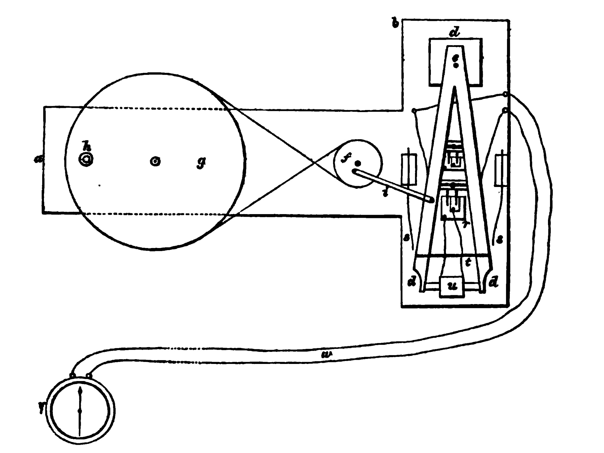
While Kepler’s conviction of the relationship between the motion of the planets and processes on Earth helped inspire our modern way of thinking, he was of course mistaken in making the association between gravity and a “simple magnetic force”. However, even this mistake was an inspired effort to describe the world around us in terms of physical causes. The universality of physical principles quickly became a central theme in the development of physics and an inspiration for Newton and those that followed. This expectation of the universality of celestial and terrestrial processes and Kepler’s expectation of universality in a connection between magnetism and the motion of the planets is evident in Faraday’s experimental investigations. Some time around the 1850’s Faraday conducted experiments to demonstrate the possible connection between the gravitational field and the electromagnetic field. Faraday constructed an experimental apparatus in an effort to measure the magnitude of electromagnetic induction associated with a gravitational field as shown in Fig. 1. Faraday’s results failed to demonstrate any relation between gravity and electricity but his commitment to this idea of universality was unwavering, Faraday1885 , “Here end my trials for the present. The results are negative. They do not shake my strong feeling of the existence of a relation between gravity and electricity, though they give no proof that such a relation exists.”

While Faraday’s experiments were not successful, later theoretical research by Skobelev Skobelev75 in 1975 supported Faraday’s “strong feeling” by demonstrating a non-zero amplitude for the interaction of gravitons and photons in both scattering and annihilation. This association between gravity and electromagnetism was also described around the same time by Gibbons gibbons in noting that, “Indeed since a ‘graviton’ presumably in some sense carries light-like momentum the creation of one or more particles with time-like or light-like momentum would violate the conservation of momentum unless the created particles were massless and precisely aligned with the momentum of the graviton”. These kinematic restrictions for conversion of massless particles have also been studied more recently and in greater detail by Fiore and Modanese Fiore96 ; Modanese95 . The processes of graviton and photon interaction described by Skobelev and Gibbons are exceedingly small Skobelev75 but are non-zero. Our more recent research has expanded on this interaction of gravity/gravitons and electromagnetism/photons through annihilation and scattering processes by recognizing the contribution of the external gravitational field associated with a gravitational wave Jones15 ; Jones16 ; Jones17 ; Jones18 ; Gretarsson18 . Our study of the vacuum production of light by a gravitational wave differs from Skobelev in that the amplitudes of the “tree level diagrams” would be dependent on the strength of the external gravitational field or equally the strain amplitude of the gravitational wave. This type of semi-classical conversion process between gravitational and electromagnetic fields was described more broadly by Davies Davies01 “One result is that rapidly changing gravitational fields can create particles from the vacuum, and in turn the back-reaction on the gravitational dynamics operates like a damping force.” The back-reaction on the gravitational wave was shown to be small compared to the gravitational wave luminosity but sufficient to be detectable under the right circumstances Jones17 .

In this brief review we will specifically outline the relationship between gravity and electricity for the special case of gravitational and electromagnetic radiation. While we take a historical perspective leading to current research no effort will be made to present the historical formalism. Instead we will present the ideas relating the association between gravitational and electromagnetic radiation and in particular the vacuum production of electromagnetic radiation by a gravitational wave using modern notation and mathematical formalism.

II Electromagnetism and light

A general review of the research on the relationship between gravity and electricity would completely preclude any possibility of being brief. We will instead focus our attention on the radiation regimes. The current understanding of the radiation regime for electricity began with James Clerk Maxwell’s modification of Ampere’s law Maxwell2 to include the displacement current. This modification led to a wave equation solution to the equations of electromagnetism. Maxwell immediately recognized this wave equation as a description of the phenomena of light. In keeping with our intent to discuss the historical development of gravitational wave production of electromagnetic radiation using modern notation, the equations describing electromagnetic radiation will be presented in a form that is completely covariant. The Maxwell equations are written in terms of tensor relations and will have the same form in Minkowski space and curved space-time. The physical properties of electromagnetic radiation, such as luminosity, will be developed in terms of Newman-Penrose scalars Newman61 ; Teukolsky73 , in a form that is well suited for the comparison of electromagnetic and gravitational radiation Jones17 .

In order to write the field equations for electrodynamics in a suitable form for curved space-time two tensors are defined in terms of the electric and magnetic fields. The field strength tensor Ellis73 ; Senego98 ; Hogan09 ; Palenzuela10 ; Lehner09 ; Lehner12_85 ; Lehner12_86 ; Lehner16 is defined as

$$F^{\mu\nu}=u^{\mu}E^{\nu}-u^{\nu}E^{\mu}+e^{\mu\nu\alpha\beta}B_{\alpha}u_{\beta},$$ (1)

and the dual to the field strength tensor as,

$${}^{*}F^{\mu\nu}=u^{\mu}B^{\nu}-u^{\nu}B^{\mu}-e^{\mu\nu\alpha\beta}E_{\alpha}u_{\beta},$$ (2)

where $e^{\mu\nu\alpha\beta}$ is the “Levi-Civita pseudotensor of the space-time” and $u_{\nu}$ is the field frame 4- velocity. The covariant expression for the field strength tensor (1) and the dual (2) was originally developed by Ellis Ellis73 . While these expressions are perhaps not widely known, expanding (1) in a Lorentz inertial frame produces the expected components for the field strength tensor. This covariant form of the field strength tensor has proven to be very useful in studies of the relation between gravity and electromagnetism Hogan09 ; Palenzuela10 ; Lehner09 ; Lehner12_85 ; Lehner12_86 ; Lehner16 . Conversely, the electric and magnetic fields are found from the contractions of the tensors with the 4-velocity,

$$E^{\mu}=F^{\mu\nu}u_{\nu},~{}~{}B^{\mu}={{}^{*}}F^{\mu\nu}u_{\nu}.$$ (3)

Using the field strength tensor and its dual the Maxwell equations can be written in a covariant form that is the same in both Minkowski space and curved space-time. The inhomogeneous Maxwell equations (i.e. Gauss’s law and Ampere’s) law are,

$$\frac{1}{\sqrt{-\left|g_{\mu\nu}\right|}}\partial_{\nu}\left(\sqrt{-\left|g_{\mu\nu}\right|}F^{\mu\nu}\right)=4\pi J^{\mu}.$$ (4)

where $\left|g_{\mu\nu}\right|=det[g_{\mu\nu}]$ is the determinant of the metric. The homogeneous Gauss’s law for magnetism and Faraday’s law are Greiner96 ; Palenzuela10 ,

$$\partial_{\nu}\left(\sqrt{-\left|g_{\mu\nu}\right|}~{}{{}^{*}}F^{\mu\nu}\right)=0.$$ (5)

The covariant form of the conservation law is,

$$\partial_{\mu}\left(\sqrt{-\left|g_{\mu\nu}\right|}J^{\mu}\right)=0.$$ (6)

The field strength tensor can also be expressed in terms of the electromagnetic 4-vector potential,

$$F_{\mu\nu}=\partial_{\mu}A_{\nu}-\partial_{\nu}A_{\mu}~{}.$$ (7)

Maxwell came to the wave equation from the bottom up by recognizing that the displacement current term was missing from the traditional form of Ampere’s law. In the modern notation the wave equation is a mathematical identity in the absence of source terms in the Maxwell equations Tsaga05 .

The covariant form of the equations for the electromagnetic field appears naturally in the radiative expression for electrodynamics in the Newman-Penrose formalism Newman61 ; Teukolsky73 through the introduction of the Newman-Penrose electromagnetic scalar, to be discussed shortly. In order to provide a means of comparison between electromagnetic and gravitational radiation using the Newman-Penrose formalism we will require the Lagrangian density for the electromagnetic field in curved space-time. Including the electric source terms the Lagrangian density is,

$$\mathcal{L}_{em}=-\frac{1}{4}\left({\partial_{\nu}A_{\mu}-\partial_{\mu}A_{\nu}}\right)\left({\partial^{\nu}A^{\mu}-\partial^{\mu}A^{\nu}}\right)+J_{\mu}A^{\mu}.$$ (8)

The Lagrangian density can be simplified using the Lorenz gauge Greiner96 , $\partial_{\mu}A^{\mu}=0$, and by restricting our attention to be source free (i.e. $J_{\mu}=0$) so that (8) becomes,

$$\mathcal{L}_{em}=-\frac{1}{2}\partial_{\mu}A_{\nu}\partial^{\mu}A^{\nu}.$$ (9)

Since we are only considering the radiation regime for the field equations, we assume a plane wave solution for the electromagnetic field and a massless vector field can then be expressed in terms of a mode expansion Greiner96 as follows,

$$A_{\mu}\left({k,\lambda,x}\right)=\epsilon_{\mu}^{(\lambda)}\phi^{(\lambda)}\left({k,x}\right).$$ (10)

with $k$ being the momentum, $x$ being the space-time coordinates and $\epsilon^{(\lambda)}$ being the polarization vectors with $\lambda=0,1,2,3$. For example, the two transverse modes are often labeled $\lambda=1,2$ with $\epsilon_{\mu}^{(1)}=(0,1,0,0)$ and $\epsilon_{\mu}^{(2)}=(0,0,1,0)$. The $\lambda=0,3$ components are the time-like and longitudinal polarizations. The four polarization vectors satisfy the orthogonality relationship $\epsilon_{\mu}^{(\lambda)}\epsilon^{\mu~{}(\lambda^{\prime})}=\eta^{\lambda\lambda^{\prime}}$, with $\eta^{\lambda\lambda^{\prime}}$ being the Minkowski metric.

One can define a complex scalar field using the $\lambda=1,2$ components of the real scalar fields i.e. $\phi^{(1,2)}(k,x)$ as $\varphi=\frac{1}{\sqrt{2}}(\phi^{(1)}+i\phi^{(2)})$. In terms of this complex scalar field the Lagrange density of (9) can be written as

$${\cal L}_{em}=-\partial_{\mu}\varphi\partial^{\mu}\varphi^{*}~{},$$ (11)

which is the Lagrange density for a massless complex scalar field. Below we will use a massless, complex scalar field as a stand-in for the massless photon. This substitution is justified by equation (11)

The field equations following from the Lagrange density in (11) are,

$$\frac{1}{{\sqrt{-\left|g_{\mu\nu}\right|}}}\partial_{\mu}\sqrt{-\left|g_{\mu\nu}\right|}g^{\mu\nu}\partial_{\nu}\varphi=0.$$ (12)

This expression for the field equations is the same for both curved space-time and for Minkowski space-time. If we restricted our attention to plane waves propagating in Minkowski space-time the solution to (12) takes the form,

$$\varphi=Be^{i\text{k}u}+C,$$ (13)

where the $z$ axis is assumed to be along the direction of propagation, $B$ and $C$ are constants, and $k$ is the wave number. The solution (13) is written in the standard light cone coordinate $u=z-t$ and $\partial_{z}-\partial_{t}=2\partial_{u}$ Jones16 .

The previous discussion provides an outline of Maxwell’s electromagnetic radiation in modern covariant form. The principle goal of this review is to realize Faraday’s expectation of a relationship between gravity and electricity. We will demonstrate this relationship for gravitational and electromagnetic radiation by comparing the gravitational radiation luminosity to the luminosity of the corresponding electromagnetic radiation produced from the vacuum by the gravitational radiation. We have found that the Newman-Penrose formalism is a good method for calculating the luminosity of both gravitational radiation and the corresponding electromagnetic radiation. The electromagnetic luminosity is presented here in terms of the Newman-Penrose formalism and the gravitational radiation luminosity will be presented in the following section.

The radiated electromagnetic power per unit solid angle is found from the projection of the electromagnetic field strength onto the elements of a null tetrad ($l_{\mu},m^{\mu},n^{\mu},\bar{m}^{\mu}$) which gives us the electromagnetic Newman-Penrose scalar $\Phi_{2}$. In the Newman-Penrose formalism the power per unit solid angle of emission for electromagnetic radiation is written as Teukolsky73 ; Lehner09 ,

$$\frac{dE_{em}}{dtd\Omega}=\mathop{lim}\limits_{r\to\infty}\frac{{r^{2}}}{{4\pi}}\left|{\Phi_{2}}\right|^{2}.$$ (14)

The Newman-Penrose electromagnetic scalar in (14) Newman61 ; Teukolsky73 ; Lehner09 ; Lehner12_86 is,

$$\Phi_{2}=F_{\mu\nu}\bar{m}^{\mu}n^{\nu}.$$ (15)

The null tetrad of the Newman-Penrose formalism in (15) can be defined as Lehner12_85 ,

$$\begin{array}[]{*{20}c}{l^{\mu}=\frac{1}{{\sqrt{2}}}\left({1,0,0,1}\right),}&{n^{\mu}=\frac{1}{{\sqrt{2}}}\left({1,0,0,-1}\right),}\\ {m^{\mu}=\frac{1}{{\sqrt{2}}}\left({0,1,i,0}\right),}&{\bar{m}^{\mu}=\frac{1}{{\sqrt{2}}}\left({0,1,-i,0}\right),}\\ \end{array}$$ (16)

and

$$l\cdot n=-1,~{}~{}m\cdot\bar{m}=1,~{}~{}l\cdot l=n\cdot n=m\cdot m=\bar{m}\cdot\bar{m}=0.$$ (17)

The electromagnetic field strength tensor in (15) is $F_{\mu\nu}=\partial_{\mu}A_{\nu}{\kern 1.0pt}-\partial_{\nu}A_{\mu}$, where $A_{\mu}=\epsilon^{(\lambda)}_{\mu}\phi^{(\lambda)}\left({t,z}\right)$, and the plane polarization vectors are $\epsilon^{(1)}_{\mu}=\left(0,1,0,0\right),\;\epsilon^{(2)}_{\mu}=\left(0,0,1,0\right)$ Jones17 . The electric and magnetic fields are determined by taking the derivatives of the scalar field (13): $\,\partial_{t}\varphi=-ikBe^{ik\left({z-t}\right)}$ and $\partial_{z}\varphi=ikBe^{ik\left({z-t}\right)}$. Collecting terms for the Newman-Penrose scalar of the “out” state of (13) Lehner12_85 ; Jones17 ,

$$\Phi_{2}=F_{\mu\nu}\bar{m}^{\mu}n^{\nu}=\frac{1}{{\sqrt{2}}}e^{-i\frac{\pi}{4}}\left({\partial_{z}\varphi-\partial_{t}\varphi}\right)=ie^{-i\frac{\pi}{4}}{\sqrt{2}}kBe^{ik\left({z-t}\right)}.$$ (18)

The square of the electromagnetic scalar is then,

$$\left|{\Phi_{2}}\right|^{2}=2k^{2}B^{2}.$$ (19)

The square of the Newman-Penrose scalar in (19) is proportional to the electromagnetic flux, $F_{em}\sim\left|{\Phi_{2}}\right|^{2}$. In Section III on gravitational radiation and in Section V.1 on scalar field production we will show that by using the Newmam-Penrose scalars for the gravitational and the electromagnetic fields respectively, one can compare the fluxes of gravitational and electromagnetic radiation Jones17 .

III Gravitational radiation

A wave like solution to the vacuum equations for general relativity exist similar to that of electromagnetism Schutz00 . This was recognized by Einstein soon after the development of general relativity and proposed even earlier by Poincaré Smoot16 . Initially there was doubt as to whether or not gravitational waves were physically real. Unlike the production of electromagnetic radiation there is no dipole source for gravitational radiation. This is because mass dipole production of radiation would violate conservation of 4-momentum Schutz00 ; Smoot16 . However, there are also quadrupole source terms which lead to a wave solution and does not violate any conservation principles Schutz00 .

Since our interest here is in the relation between gravity and electromagnetism, in the radiation regime, we will restrict our attention to the plane wave solution of general relativity. The metric of a gravitational plane wave traveling in the $+z$ direction and with the $+$ polarization can be written as Schutz ,

$$ds^{2}=g_{\mu\nu}dx^{\mu}dx^{\nu}=-dt^{2}+dz^{2}+f^{2}dx^{2}+g^{2}dy^{2},$$ (20)

were we set $c=1$. This metric is oscillatory with $f=1+\varepsilon(u)$, $g=1-\varepsilon(u)$ with $\varepsilon(u)=h_{+}e^{iku}$. The coefficient $h_{+}$ is the gravitational wave strain amplitude and $k$ is the wave number. The coordinate variable in the metric is the standard light cone coordinate $u=z-t$. This metric only includes the “plus” polarization. Similar to electromagnetic radiation there are two degrees of freedom corresponding to two polarization states for gravitational radiation. The two polarization states for gravitational radiation are “plus” and “cross” polarization. They differ by an angle of $\frac{\pi}{4}$ in contrast to a phase angle difference of $\frac{\pi}{2}$ for electromagnetism Schutz00 ; Schutz09 . Including the “cross” polarization would not change our discussion.

Figure 2: The “discovery paper” spectrogram of gravitational waves produced by a binary black hole in-spiral LIGO .

The luminosity of the gravitational radiation can be calculated using the Newman-Penrose formalism Teukolsky73 ; Lehner09 . The relevant scalar for gravitational radiation is a projection of the Riemann tensor onto elements of a null tetrad. This projection is identified as the gravitational Newman-Penrose scalar $\Psi_{4}$. The power per unit of solid angle for the gravitational radiation is written in terms of the gravitational scalar as,

$$\frac{dE_{gw}}{dtd\Omega}=\mathop{lim}\limits_{r\to\infty}\frac{{r^{2}}}{{16\pi k^{2}}}\left|{\Psi_{4}}\right|^{2}.$$ (21)

Substituting the metric for the gravitational wave (20) into the Riemann tensor for an outgoing gravitational plane wave in vacuum the gravitational Newman-Penrose scalar Teukolsky73 ; Jones17 is,

$$\Psi_{4}=-R_{\alpha\beta\gamma\delta}n^{\alpha}\bar{m}^{\beta}n^{\gamma}\bar{m}^{\delta}=f\partial_{u}^{2}f-g\partial_{u}^{2}g.$$ (22)

The partial derivatives, $\partial_{u}$, are with respect to the light cone coordinate, $u$. For the plane wave metric, where $\varepsilon=h_{+}e^{iku}$, the gravitational Newman-Penrose scalar and the square are given by,

$$\Psi_{4}=-2h_{+}k^{2}e^{ik\left({z-t}\right)}\rightarrow|\Psi_{4}|^{2}=4h_{+}^{2}k^{4}.$$ (23)

The Newman-Penrose scalars in (19) and (23) provide a convenient method for the comparison of the power of the gravitational radiation and the counterpart vacuum production of electromagnetic radiation which will follow. The flux of the gravitational wave can be calculated from (21) and (22) as Schutz ; Schutz09 ; Gretarsson18 ,

$$F_{gw}=\frac{c^{3}}{16\pi G}\left|\dot{\varepsilon}\right|=\frac{c^{3}h_{+}^{2}\omega^{2}}{16\pi G},$$ (24)

which is a function of the strain amplitude $h$ and gravitational wave frequency $\omega=2\pi f$.

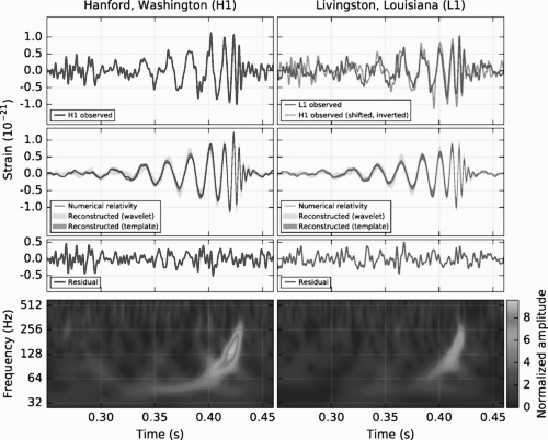
This review of the relationship between gravity and electromagnetism in the radiation regime might be considered of academic interest only except for the recent and remarkable discovery by the LIGO scientific collaboration of gravitational waves LIGO . The spectrogram from the discovery papers is provided in Fig. 2 for the binary in-spiral of two black holes. The detection of gravitational waves makes the discussion of the potential production of electromagnetic radiation by gravitational waves immediately relevant to current research in both the fundamental relation between gravity and electromagnetism as well as potential applications in astrophysics. If there were any lingering doubt about the certainty of the detection of gravitational waves the more recent detection of gravitational waves from a kilonova event ligo2 has laid these doubts to rest. The kilonova event was first identified through the detection of gravitational waves by the LIGO scientific collaboration. The kilonova was immediately verified across the electromagnetic spectra through the coordination of an international collaboration of observatories based around the World and in space. The kilonova observations have not only eliminated any reasonable doubt of the existence of gravitational waves but also ushered in a new era of “multi-messenger” astronomy and astrophysics.

IV Electromagnetic fields in gravitational wave background

IV.1 Gravitational waves and uniform magnetic field

The first modern attempt to connect gravitational radiation and electromagnetic fields was work by Gertsenshtein Gertsenshtein60 which considered the linearized Einstein field equations coupled to an electromagnetic plane wave.

$$\Box{\tilde{h}}^{\mu\nu}=-\kappa t^{\mu\nu}~{},$$ (25)

where $t^{\mu\nu}=\frac{1}{4\pi}(F^{\mu\tau}F^{\nu}_{\tau}-g^{\mu\nu}F^{\alpha\beta}F_{\beta\alpha})$ is the energy-momentum tensor for the electromagnetic field, ${\tilde{h}}^{\mu\nu}=h^{\mu\nu}-\frac{1}{2}g^{\mu\nu}h$ is the trace reduced metric deviation of the metric tensor (i.e. $g^{\mu\nu}=\eta^{\mu\nu}+h^{\mu\nu}$), and $\kappa=16\pi G$. Now the proposal in Gertsenshtein60 was to generate gravitational waves by sending electromagnetic waves through a constant magnetic field. This potential effect was compared to radio physics phenomenon of wave resonance. The idea being that despite the weak coupling of gravity one could nevertheless generate some significant amount of gravitational radiation by this method.

Now if one takes the electromagnetic field to have a constant magnetic field part (whose field strength tensor we denote by $F^{(0)\mu\nu}$) and a plane wave part (whose field strength we denote by $F^{\mu\nu}$), and if we feed this into (25), dropping the squared terms in $F^{(0)\mu\nu}$ and $F^{\mu\nu}$ and keeping only the cross terms we arrive at

$$\Box{\tilde{h}}^{\mu\nu}=-\frac{\kappa}{2}\left(F^{(0)\mu\tau}F^{\nu}_{\tau}-\frac{1}{4}g^{\mu\nu}F^{(0)\alpha\beta}F_{\alpha\beta}\right)~{}.$$ (26)

One now assumes that the electromagnetic plane wave field and gravitational field propagate along the $z$ direction with wave number $k$ and have the form

$$F^{\mu\nu}=b(z)\epsilon^{\mu\nu}e^{i(kz-\omega t)}~{}~{}~{};~{}~{}~{}{\tilde{h}}^{\mu\nu}=a(z)\zeta^{\mu\nu}\sqrt{\frac{\kappa}{k^{2}}}e^{i(kz-\omega t)}~{},$$ (27)

where $\epsilon^{\mu\nu},\zeta^{\mu\nu}$ are the electromagnetic and gravitational polarization tensors respectively. Using (27) in (26) and assuming slowly varying amplitudes $a(z),b(z)$ one obtains the following relationship between the amplitudes

$$i\frac{da(z)}{dz}=\sqrt{\frac{\kappa}{16}}F^{(0)\mu\nu}\epsilon_{\beta\nu}\zeta^{\beta}_{\mu}b(z)~{}.$$ (28)

Under the assumption that $b(x)\approx const.$ (28) can be integrated to obtain $a(x)$ as

$$\left|\frac{a(z)}{b(0)}\right|^{2}=\frac{\kappa}{16\pi^{2}}B_{0}^{2}T^{2}~{},$$ (29)

where $B_{0}\simeq|F^{(0)\mu\nu}|$ is the constant magnetic field strength, $T$ is the time that the electromagnetic wave traverses the uniform magnetic field, and $b(0)$ is the initial amplitude of the electromagnetic wave. If one takes the cosmological sized magnetic fields ($B_{0}\simeq 10^{-5}$ G) and assumes cosmological times for the electromagnetic wave to travel through this constant magnetic field ($T\simeq 10^{7}$ years) one finds that the ratio of gravitational to electromagnetic amplitude is of the order $|a/b|^{2}\simeq 10^{-17}$. One could increase this by having stronger magnetic fields and/or longer periods of travel.

One of the most interesting features of the above mechanism is that the gravitational wave frequency is the same as that of the electromagnetic wave. This gives the possibility of generating very high frequency gravitational waves compared to the “natural” sources of gravitational waves from the first series of direct detections– merging black hole, merging neutron stars. These natural or astrophysical sources have frequencies in the 100s to 1000s of Hertz, whereas electromagnetic radiation has a much broader range of frequencies which have been observed – from 1000s of Hertz to Gigahertz and beyond.

In the original work by Gertsenshtein Gertsenshtein60 the focus was on generating gravitational waves from electromagnetic waves. In this review our focus is the exact opposite – we are interested in electromagnetic radiation generated from gravitational waves. This reversed possibility was pessimistically noted by Gertsenshtein with the concluding comment “From general relativity follows also the possibility of the inverse conversion of gravitational waves into light waves, but this problem is hardly of interest.” Nevertheless, several years after Gertsenshtein’s paper, Lupanov lupanov67 did examine the inverse process of generating electromagnetic waves from gravitational waves.

We will follow the work in lupanov67 by examining the reverse process of electromagnetic radiation generated from gravitational waves. There are two reasons for our focus on the reverse process: (i) electromagnetic radiation, even weak radiation, is easier to detect, and (ii) we argue, beginning in the next subsection, that the conversion of gravitational waves to electromagnetic radiation occurs even in vacuum.

Before concluding this subsection we mention that there is more recent work in the spirit of Gertsenshtein’s work Gertsenshtein60 where the magnetic field is replaced by a Bose-Einstein condensate fuentes . In this case the interaction of the gravitational wave with the Bose-Einstein condensate is conjectured to lead to the creation of phonons, just as in Gertsenshtein’s work the interaction of the gravitational wave with the magnetic field lead to the creations of photons. This creation of phonons with a Bose-Einstein condensate has been put forward as a potential alternative mechanism to interferometers like LIGO to detect gravitational waves.

IV.2 Feynman diagram approach to gravitational and electromagnetic radiation

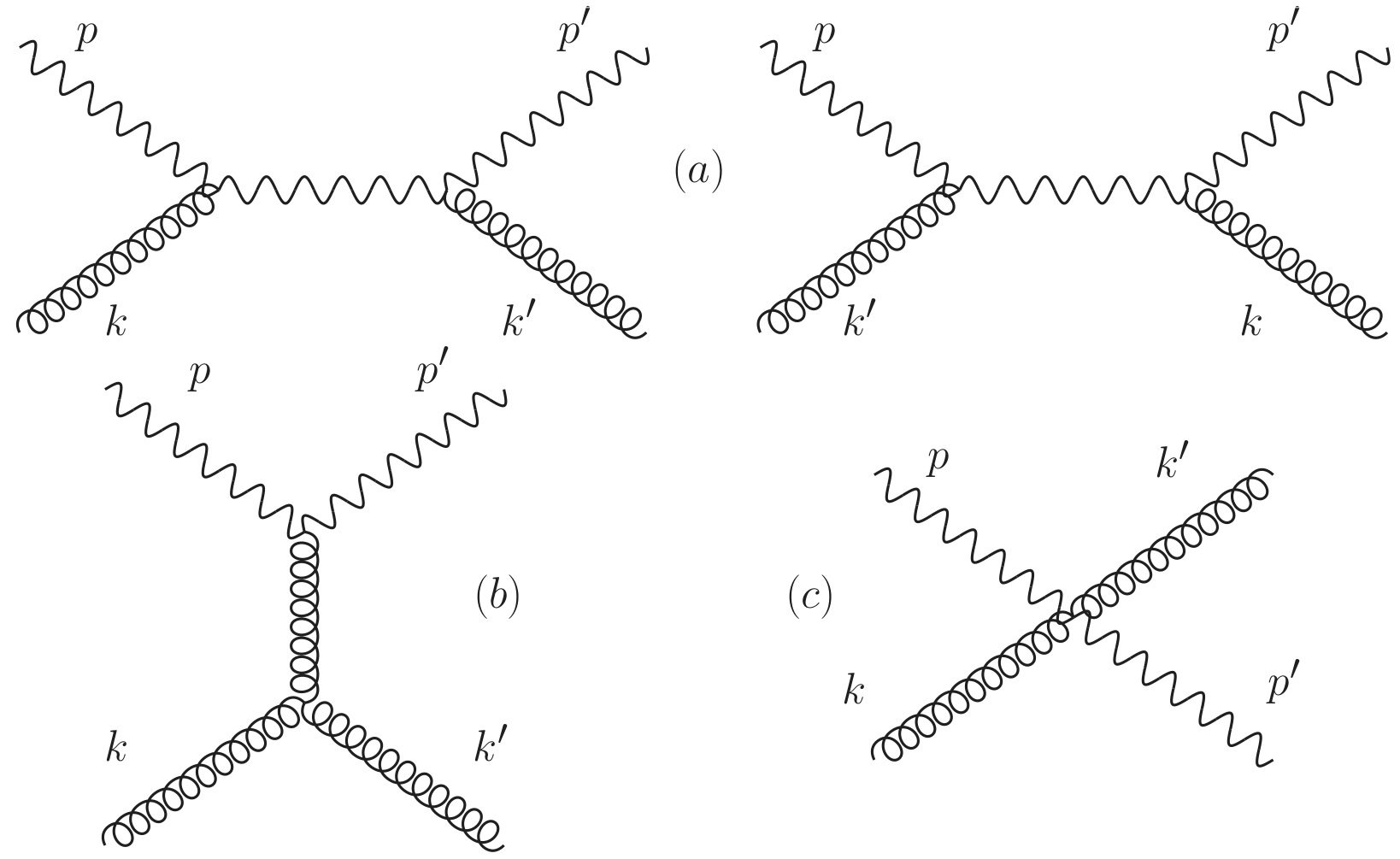
To check the assertion that electromagnetic radiation can be created in vacuum from gravitational radiation we turn to tree-level Feynman diagrams for graviton-photon scattering. The four basic diagrams for this process are given in Fig. (3) with curly lines representing gravitons and wavy lines represent photons. The original calculation was carried out by Skobelev Skobelev75 with more recent and more extensive calculations being found in references Bohr14 . The diagrams in Fig. (3) represent $graviton+photon\to graviton+photon$ scattering. By rotating the diagrams one can get $graviton+graviton\to photon+photon$ or $photon+photon\to graviton+graviton$ which can be viewed as creation of photons (gravitons) from gravitons (photons).

Figure 3: Tree level Feynman diagrams of graviton-photon transitions Skobelev75 . Wavy lines represent photons and curly lines represent gravitons

In Skobelev75 the process $graviton+photon\to graviton+photon$ is calculated first. After a long calculation the differential scattering cross section is found to be

$$\frac{d\sigma}{d\cos\Theta}=\frac{\kappa^{2}\omega^{2}}{64\pi}\left(\frac{1+\cos^{8}(\Theta/2)}{\sin^{4}(\Theta/2)}\right)~{},$$ (30)

where $\kappa=16\pi G$ as previously, $\omega$ is the energy of the system, and $\Theta$ is the scattering angle.

Now the process of interest in this review is where gravitational waves create electromagnetic waves or photons. In the Feynman diagram language this means $graviton+graviton\to photon+photon$. This process can be obtained by rotating the diagrams in Fig. 3 by $90^{0}$ degrees. Upon doing this the differential cross section for $graviton+graviton\to photon+photon$ is found to be Skobelev75

$$\frac{d\sigma}{d\cos\Theta}=\frac{\kappa^{2}\omega^{2}}{64\pi}(\cos^{8}(\Theta/2)+\sin^{8}(\Theta/2))~{}.$$ (31)

Integrating (31) to obtain the total cross section

$$\sigma=\frac{\kappa^{2}\omega^{2}}{160\pi}~{}.$$ (32)

If one takes the energy of the system to be the rest mass energy of the electron, $\omega=m_{e}c^{2}$, one finds Skobelev75 that $\sigma\simeq 10^{-110}cm^{2}$. This is a very small number and indicates that at the level of individual photons and gravitons this is not a large effect. However, given the enormous energy of the observed gravitational wave signals, which implies a large number of gravitons, we will argue that there are cases where the small cross section of (32) may be compensated for by the large number of gravitons/strength of the gravitational wave.

IV.3 Massive Scalar field in Gravitational Plane Wave Background

The idea of particle creation from a time dependent space-time was first considered in a series of papers by Parker parker-1 ; parker-2 ; parker-3 which investigated particle production from the time dependent FRW cosmological space-time. The next major time-dependent space-time to be studied in terms of particle production was the gravitational plane wave space-time. The initial studies were carried out by Gibbons gibbons and Deser deser , who considered the production of a massive scalar field in a pulsed gravitational wave space-time. Reference garriga has a more extensive discussion of particle creation from a gravitational wave background, again in the context of a massive scalar field. The conclusion of all of these works was that massive scalar fields would not be created from such a plane wave gravitational background.

This conclusion, of no particle creation from a plane gravitational wave background, appears at odds with recent work Jones15 ; Jones16 ; Jones17 ; Jones18 . However these recent works focus on the case of massless particles whereas references gibbons ; deser ; garriga focus on massive particles. As noted by Gibbons one can already guess that the production of a massive field from a gravitational plane wave would be forbidden by energy momentum conservation. A massless graviton can not decay/transform into massive particles since this would violate energy-momentum conservation. It is the same reason that forbids a photon from decaying into an electron-positron pair in free space. (A photon can decay/transform into electron-positron pair in the presence of a heavy nuclei which acts to conserve energy and momentum).

General studies of when one type of massless field quanta can decay/transform into other massless field quanta can be found in Modanese95 and Fiore96 . Using energy-momentum conservation these two works show that some number of massless quanta can transform into some number of other massless field quanta so long as the incoming and outgoing particles lie along the same direction. This is consistent with the Feynman diagram calculations of reference Skobelev75 where the decay of gravitons to photons (i.e. $graviton+graviton\to photon+photon$) is possible so long as the momenta of all particles lie along the same direction. This is also the condition under which the creation of massless fields/field quanta occurs in references Jones15 ; Jones16 ; Jones17 ; Jones18 .

In the rest of this section we review the calculations of gibbons ; deser ; garriga which demonstrate the absence of particle creation when the particles are massive, since this will provide a nice segue to the case of massless particles. We will follow the notation of reference garriga .

Garriga and Verdaguer garriga begin by considering the plane wave metric of the form

$$ds^{2}=-dt^{2}+dz^{2}+g_{ab}(z,t)dx^{a}dx^{b}=-dudv+g_{ab}(u)dx^{a}dx^{b}~{},$$ (33)

where in the last expression the metric has been transformed to light front coordinates defined as $u=z-t$ and $v=z+t$ with $c=1$. The indices $a,b=1,2$ and run over the $x,y$ directions, which are perpendicular to the $+z$ direction of travel of the gravitational wave. For a gravitational wave traveling in the $-z$ direction one would take the metric components to be functions of the light front coordinate $v$ i.e. $g_{ab}(v)$.

Next a massive scalar field, $\varphi$, is placed in the metric given by (33). The equation for a massive scalar field in a curved background is given by

$$\left[\frac{1}{{\sqrt{-\left|{g_{\mu\nu}}\right|}}}\left({\partial_{\mu}g^{\mu\nu}\sqrt{-\left|{g_{\mu\nu}}\right|}\partial_{\nu}}\right)-m^{2}\right]\varphi=0.$$ (34)

Using the metric (33) in equation (34) and applying separation of variables, one finds solutions for the scalar field of the form

$$\varphi(u,v,x^{a})=\frac{1}{(p_{-})^{1/2}(detg_{ab}(u))^{1/4}(2\pi)^{3/2}}\exp\left[ip_{a}x^{a}-ip_{-}v-\frac{i}{4p_{-}}\int_{0}^{u}(g_{ab}p^{a}p^{b}+m^{2})du\right]~{},$$ (35)

with $p_{-}$ and $p_{a}$ being separation constants which physically correspond to momenta connected with the coordinates, $v$ and $x^{a}$ respectively.

The next step is to calculate the Bogoliubov coefficients davies for this scalar field for a sandwich space-time i.e. one has a plane wave space-time for $u_{1}<u<u_{2}<0$, sandwiched between two Minkowski space-times for $u<u_{1}$ and $u>u_{2}$. The “in” and “out” states for this sandwich space-time are garriga

$$\varphi^{in}(u,v,x^{a}) = \frac{1}{(p_{-})^{1/2}(2\pi)^{3/2}}\exp\left[ip_{a}x^{a}-ip_{-}v-\frac{i}{4p_{-}}(p_{a}p^{a}+m^{2})u+i\Delta\right]~{},$$ (36)

$$\varphi^{out}(u,v,x^{a}) = \frac{1}{(k_{-})^{1/2}(2\pi)^{3/2}}\exp\left[ik_{a}x^{a}-ik_{-}v-\frac{i}{4k_{-}}(k_{a}k^{a}+m^{2})u\right]~{},$$ (37)

where $\Delta$ is a constant phase. For the exact expression for this phase as well as for the full details of the calculation and some subtleties in the definition of the coordinates we refer the reader to garriga . The light front momentum $p_{-}$ and $k_{-}$ are given by

$$p_{-}=\frac{\omega_{p}-p_{z}}{2}~{}~{}~{};~{}~{}~{}k_{-}=\frac{\omega_{k}-k_{z}}{2}~{},$$ (38)

with $p_{z},k_{z}$ being the three-momentum in the $z$ direction and $\omega_{p}=\sqrt{{\bf p}^{2}+m^{2}}$ and $\omega_{k}=\sqrt{{\bf k}^{2}+m^{2}}$ are the energies associated with the wave solutions.

From (36) and (37) one can calculate the Bogoliubov beta coefficients to be

$$\beta=-\langle\varphi^{in}|\varphi^{out~{}*}\rangle\propto\delta(p_{-}+k_{-})~{},$$ (39)

with the Dirac delta being a function of $p_{-},k_{-}$ coming from integration over $dv$. Now if the scalar field is massive it is easy to see, using the expressions for $\omega_{p}\omega_{k}$ in equation (38) that $p_{-}+k_{-}\neq 0$ so that $\beta=0$. However, if $m=0$ and the 3- momentum are in the same direction ${\bf p}=p_{z}={\bf k}=k_{z}$ then $p_{-}+k_{-}=0$ and $\beta\neq 0$ meaning that production of the scalar field from the gravitational wave occurs. This is consistent with the Feynman diagram calculations of Skobelev75 ; Bohr14 as well as the discussion in term of energy-momentum conservation of particle decay/production/scattering of massless fields Modanese95 ; Fiore96 . In the next section we investigate in more detail the possibility of producing massless fields/particles from a gravitational wave background.

V Particle Production from a Gravitational Wave Background

In this section we review some recent work Jones15 ; Jones16 ; Jones17 ; Jones18 on the production of massless fields from gravitational wave backgrounds. We use a massless scalar field to carry out the analysis, but our results also apply to the more realistic case of a massless vector field from the results and discussion around equations (8), (9), (10), and (11). We also look at the response of an Unruh-Dewitt detector in a gravitational plane wave background which supports the picture of gravitons decaying/transforming into photons.

V.1 Scalar field production

We now repeat some of the calculations of the previous section but for a massless scalar field. We will follow the work of Jones16 . For the gravitational plane wave background we take the metric of (33) to have the more specific form

$$ds^{2}=-dt^{2}+dz^{2}+f^{2}(z,t)dx^{2}+g^{2}(z,t)dy^{2}=-dudv+f^{2}(u)dx^{2}+g^{2}(u)dy^{2}~{},$$ (40)

where we have again transformed to light front coordinates, $u,v$ and taken $c=1$. The form of the metric in (40) assumes the plus-polarization for the gravitational plane wave, which we take without loss of generality. We further assume that the ansatz functions have a oscillatory behavior of the form $f(u)=1+h_{+}e^{iku}$ and $g(u)=1-h_{+}e^{iku}$, where $h_{+}$ is the dimensionless amplitude of the plus polarization and $k$ is the gravitational wave number. With $m=0$ the field equation for $\varphi$ from (34) becomes

$$\frac{1}{{\sqrt{-\left|{g_{\mu\nu}}\right|}}}\left({\partial_{\mu}g^{\mu\nu}\sqrt{-\left|{g_{\mu\nu}}\right|}\partial_{\nu}}\right)\varphi=0.$$ (41)

Using the plane wave metric from (40) along with the oscillatory form of the ansatz functions $f(u),g(u)$ equation (41) becomes

$$\left({4F(ku)\partial_{u}\partial_{v}-4ikG(ku)\,\partial_{v}+H(ku)\left({\partial_{x}^{2}+\partial_{y}^{2}}\right)}\right)\varphi=0,$$ (42)

where the functions $F(ku),G(ku),H(ku)$, are given by

$$\begin{array}[]{l}\quad F\left({ku}\right)\equiv\left(1-h_{+}^{2}e^{2iku}\right)^{2},\\ \quad G\left({ku}\right)\equiv h_{+}^{2}e^{2iku}\left(1-h_{+}^{2}e^{2iku}\right),\\ \quad H\left({ku}\right)\equiv\left({1+h_{+}^{2}e^{2iku}}\right).\\ \end{array}$$ (43)

In arriving at (42) we have assumed that the behavior of $\varphi$ in the perpendicular $x,y$ directions are the same so that $\partial_{x}\varphi=\partial_{y}\varphi$ and $\partial_{x}^{2}\varphi=\partial_{y}^{2}\varphi$.

To solve (42) we employ separation of variables as $\varphi(u,v,x,y)=U(u)V(v)X(x)Y(y)$. The ansatz functions in the $v,x,y$ directions are plane waves of the form

$$X(x)=e^{ik_{xy}x}~{}~{}~{};~{}~{}~{}Y(y)=e^{ik_{xy}y}~{}~{}~{};~{}~{}~{}~{}V(v)=e^{ik_{v}v}~{},$$ (44)

where we have enforced the equality of the $x$ and $y$ directions by taking a common wave number, $k_{xy}$. With this set up and the solutions from (44) the solution for $U(u)$ is Jones16

$$U=Be^{\frac{\lambda}{k}}e^{\frac{-\lambda}{{k\left({1-h_{+}^{2}e^{2iku}}\right)}}}\left({1-h_{+}^{2}e^{2iku}}\right)^{\frac{1}{2}\left({\frac{\lambda}{k}-1}\right)}e^{-i\lambda u}+C~{},$$ (45)

with $B,C$ being integration constants and $\lambda=\frac{k_{xy}^{2}}{2k_{v}}$. Putting equations (44) (45) together, and taking $C=-B$ the scalar field in the plane wave background becomes

$$\varphi(u,v,x,y)=Be^{\frac{\lambda}{k}}e^{-\frac{\lambda}{{k\left({1-h_{+}^{2}e^{2iku}}\right)}}}\left({1-h_{+}^{2}e^{2iku}}\right)^{\frac{1}{2}\left({\frac{\lambda}{k}-1}\right)}e^{-i\lambda u}e^{ik_{v}v}e^{ik_{xy}x}e^{ik_{xy}y}-B.$$ (46)

In the limit $h_{+}\to 0$ (i.e. the gravitational background is turned off) the scalar field in (46) becomes

$$\varphi_{0}(t,x,y,z)=Be^{-i\lambda u}e^{ik_{v}v}e^{ik_{xy}x}e^{ik_{xy}y}-B\rightarrow Be^{i\left({k_{v}+\lambda}\right)t}e^{i\left({k_{v}-\lambda}\right)z}e^{ik_{xy}x}e^{ik_{xy}y}-B~{},$$ (47)

where in the last step we have converted back to the original $t,x,y,z$ coordinates. One can see that $k_{v}+\lambda$ plays the role of the wave energy and $k_{v}-\lambda$ momentum in the $z$ direction. The result in (47) is expected, since if the gravitational wave background is turned off one should recover a plane wave traveling in free space, which is what the solution in (47) represents.

Taking the limit where all the wave numbers/momenta go to zero (i.e. $k_{v},\lambda,k_{xy}\to 0$) in equation (46) one would expect the scalar field to vanish. However on taking this limit one finds instead that

$$\varphi(u,v,x,y)=B\left[\left({1-h_{+}^{2}e^{2iku}}\right)^{-\frac{1}{2}}-1\right]\approx\frac{B}{2}h_{+}^{2}e^{2iku}+\frac{3B}{8}h_{+}^{4}e^{4iku}~{}.$$ (48)

The result in (48) shows that even when one tries to take the wave to its vacuum state, namely $k_{v},\lambda,k_{xy}\to 0$, there is a non-vanishing and non-trivial scalar field. This non-vanishing scalar field is the field/field quanta created by the gravitational wave background. Note that if one takes $h_{+}\to 0$ in (48) that one does get the expected value for the scalar field $\varphi\to 0$ The four-current associated with $\varphi$ is given by the standard expression $j_{\mu}=-i(\varphi\partial_{\mu}\varphi^{*}-\varphi^{*}\partial_{\mu}\varphi)$. Inserting this solution from (46) in the expression for the four-current and time averaging gives Jones16

$$\langle j_{\mu}\rangle=-2B^{2}\lambda-B^{2}h_{+}^{4}\left(\frac{9}{2}\frac{\lambda^{3}}{k^{2}}-\frac{12\lambda^{2}}{k}+\frac{13}{2}\lambda-k\right)~{}.$$ (49)

The constant $B$ is determined by choosing a normalization condition or convention. Following references stahl and Jones16 we pick the normalization condition $B=\frac{1}{\sqrt{2kV}}$. Other possible normalization conditions for $B$ are discussed in halzen . With this normalization the vacuum scalar field from (48) reads

$$\varphi(u,v,x,y)=\frac{1}{\sqrt{2kV}}\left[\left({1-h_{+}^{2}e^{2iku}}\right)^{-\frac{1}{2}}-1\right]\approx\frac{1}{2\sqrt{2kV}}h_{+}^{2}e^{2iku}\left(1+\frac{3}{4}h_{+}^{2}e^{2iku}\right)~{}.$$ (50)

Time averaging this vacuum current from (49) gives

$$\langle j_{\mu}\rangle=\frac{\rm{sign}(k)h_{+}^{4}}{2V}~{}.$$ (51)

In (50) we are using a normalization that assumes the scalar field is in a box of volume $V$. In the previous section we took $B=\frac{1}{(2\pi)^{3/2}}$ – see (36) (37).

Equation (49) gives the effect, in terms of the four-current, of passing a massless scalar field through a gravitational wave. On setting all the energy-momentum of the scalar field to zero one finds, from equations (50) and (51), that the scalar field and scalar field current do not vanish. This represents the production of scalar field/scalar field quanta from the gravitational wave background.

Following Jones17 the ratio of the produced electromagnetic radiation (14) to the gravitational (21) radiation can be written down in terms of electromagnetic and gravitational Newman-Penrose scalars from (15) and (23),

$$\frac{{dE_{em}}}{{dE_{gm}}}=\frac{{\left({\frac{1}{{4\pi}}\left|{\Phi_{2}}\right|^{2}}\right)}}{{\left({\frac{1}{{16\pi k^{2}}}\left|{\Psi_{4}}\right|^{2}}\right)}}=\frac{F_{em}}{F_{gw}}.$$ (52)

Switching to a normalization where $B=1$ in (48) the amplitude of the leading term of the scalar field is $\frac{h_{+}^{2}}{2}$. Using this in the expression for $|\Phi_{2}|^{2}$ calculated in (19) we get $|\Phi_{2}|^{2}=2k^{2}h_{+}^{4}$. Next from (23) we recall that $|\Psi_{4}|^{2}=4h_{+}^{2}k^{4}$ for a gravitational plane we. Using all this in (52) yields a relationship between the electromagnetic wave flux and gravitational wave flux

$$F_{em}=2h_{+}^{2}F_{gw}.$$ (53)

Since the gravitational radiation is proportional to $h_{+}^{2}$ the electromagnetic production will be proportional to $h_{+}^{4}$. The result in equation (53) is consistent with the result in equation (51).

V.2 Unruh-Dewitt detector approach

Another approach to study the connection between gravitational and electromagnetic radiation is through the use of an Unruh-DeWitt detector unruh-det ; dewitt-det . An Unruh-DeWitt detector is a two-state, quantum system which is placed in a given space-time background. If the Unruh-DeWitt detector is excited from the low energy state to the high energy state, this is taken to indicate that the given space-time has produced field quanta in order to excite this transition. Two common examples of the use of an Unruh-DeWitt detector are placing it in the Schwarzschild space-time davies ; hawking of a black hole or placing it the Rindler space-time of an accelerating observer unruh . In the first case the Unruh-DeWitt detector will detect the photons from Hawking Radiation and in the second case the Unruh-DeWitt detector will detect the photons from Unruh Radiation.

In this subsection we will summarize the work of reference Jones15 which calculates the response of an Unruh-DeWitt detector interacting with a plane gravitational wave. The expression for the spectrum, $S(E)$, of an Unruh-DeWitt detector is given by

$$S(E)=n_{general}-n_{inertial}=2\pi\rho(E)F(E)~{}.$$ (54)

In equation (54) $n_{general}$ and $n_{inertial}$ are the photon density of a general space-time and inertial space-time respectively. The difference between these two is a measure of the photons created due to the general space-time. The terms $\rho(E)$ and $F(E)$ are, respectively, the density of states and response function both as a function of energy davies ; letaw ; akhmedov ; wilburn ; rad .

The detector response function is given by

$$F(E)=\int_{-\infty}^{+\infty}e^{-i\Delta\tau\Delta E}(G^{+}_{general}(\Delta\tau)-G^{+}_{inertial}(\Delta\tau))d(\Delta\tau)~{},$$ (55)

where we recall that $\hbar=1$ and $c=1$ in the above formulas. $\Delta E=E_{up}-E_{down}$ is the energy difference between the two states of the Unruh-DeWitt detector. For simplicity we assume $E_{down}=0$ so that $\Delta E\to E_{up}\to E$ and thus the response function is written as just a function of $E$. The terms $G^{+}_{general}(\Delta\tau)$ and $G^{+}_{inertial}(\Delta\tau))$ are the Wightman functions davies ; Jones15 for the detector path in a general space-time and the detector path in the inertial space-time. The Wightman function depends on the proper time difference $\Delta\tau$ for the path through the given space-time. The space-time path for the inertial detector is $x^{\mu}(\Delta\tau)=(\Delta\tau,0,0,0)$. The Wightman function for this inertial detector is

$$G_{inertial}^{+}=\frac{1}{4\pi^{2}x^{\mu}x_{\mu}}=\frac{1}{4\pi^{2}\Delta\tau^{2}}~{}.$$ (56)

For a gravitational wave traveling in the $+z$ direction and having $+$ polarization the space-time path is given by $x^{\mu}(\Delta\tau)=(\gamma\Delta\tau,\Delta x,0,0)$, where $\Delta x$ is the spatial displacement of the detector due to the gravitational wave and $\gamma^{-2}=1-\Delta{\dot{x}}^{2}$. Without loss of generality the detector is taken to be aligned along the $x$ direction. The Wightman function for the gravitational wave is

$$G_{wave}^{+}=\frac{1}{4\pi^{2}x^{\mu}x_{\mu}}=\frac{1}{4\pi^{2}(\gamma^{2}\Delta\tau^{2}-\Delta x^{2})}~{}.$$ (57)

Using these two Wightman functions from (56) (57) in (55) we find

$$F(E)=\frac{1}{2\pi^{2}}\int_{0}^{+\infty}\cos(E\Delta\tau)\left(\frac{1}{(\gamma^{2}\Delta\tau^{2}-\Delta x^{2})}-\frac{1}{\Delta\tau^{2}}\right)d(\Delta\tau)~{}.$$ (58)

To evaluate (58) we need to give $\Delta x$ as a function of $\Delta\tau$. This is done using the ${\dot{x}}=(1+\frac{1}{2}h)$ EFTaylor which is the expression for the trajectory along a null geodesic, to first order, for a gravitational wave background characterized by the amplitude $h(\Delta\tau,\theta,\psi)=h_{0}\sin^{2}(\theta)\sin(2\psi)\sin(\omega\Delta\tau)$. The angles $\theta$ and $\psi$ give the orientation of the axis of the detector with respect to the incoming gravitational wave hendry . The separation $\Delta x$ between the particle undergoing geodesic motion in the gravitational wave background characterized by $h(\Delta\tau,\theta,\psi)$ and an inertial observer is then given by $\Delta x=(1+\frac{1}{2}h)\Delta\tau-\Delta\tau=\frac{1}{2}h(\Delta\tau,\theta,\psi)\Delta\tau$. Using these results in (58) and integrating over $\Delta\tau$ as well as integrating over the orientation direction $\theta$ and $\psi$ gives the detector response function as Jones15

$$F(E)=\frac{3\pi}{256}h_{0}^{2}(2\omega-E)\Theta(2\omega-E),$$ (59)

where $\Theta$ is the Heaviside step function. Thus $F(E)=0$ when $E>2\omega$ which is a similar type of cut-off to that in muon decay halzen ; griffiths . This suggests a picture of gravitons “decaying” into photons – $graviton+graviton\to photon+photon$ or $graviton\to graviton+photon+photon$.

Using the response function from (59) and a density of states $\rho(E)=\frac{E^{2}}{2\pi^{2}}$ letaw the spectrum can be found from (54) as

$$S(E)=\frac{3}{256\pi\hbar^{3}c^{3}}E^{2}h_{0}^{2}(2\hbar\omega-E)\Theta(2\hbar\omega-E)~{}.$$ (60)

We have restored factors of $\hbar$ and $c$ temporarily. The functional form of the spectrum from (60) is that of a $Beta(3,2)$ distribution which is reminiscent of particle decays. This again supports the picture of gravitons decaying into photons.

The analysis of the present subsection is different from the proceeding subsection in that here we place an Unruh-DeWitt detector in the presence of a gravitational plane wave background, whereas in the previous subsection we focused on the response of the vacuum to a gravitational wave. The Unruh-DeWitt calculation is closer in spirit to the work of Gertsenshtein Gertsenshtein60 where the gravitational wave interacts with a magnetic field. In both these cases there is some physical object – the Unruh-DeWitt detector or a magnetic field – which interacts with the gravitational wave. In the previous subsection the gravitational wave interacts with the quantum vacuum. Nevertheless all of these calculations indicate that a gravitational wave can create electromagnetic radiation, or in particle language that gravitons can transform/decay into photons. The work in Calmet16 also looks into this possibility of gravitons decaying/transforming in to photons and thus weakening the gravitational wave.

VI Possible Observational Consequences/Signatures

While gravitational waves have only been directly detected very recently, electromagnetic radiation has been observed for all of human existence. If gravitational waves produce counterpart electromagnetic radiation as is outlined above, it is natural to ask what the possible observable consequence of this would be. In this section we address two possible observational consequence: (i) the attenuation/decay of the gravitational wave due to production electromagnetic radiation; (ii) the direction detection of the electromagnetic radiation produced by the gravitational wave.

VI.1 Decay/attenuation of the gravitational wave

If electromagnetic waves are produced from a gravitational wave, as suggested above, this should weaken and attenuate the gravitational wave since this electromagnetic radiation must be created at the expense of the gravitational wave Jones15 ; Jones16 . This is similar to how a black hole is conjectured to lose mass as a result of Hawking radiation – the Hawking radiation comes at the expense of the mass of the black hole.

One can connect particle/field production rate, $\Gamma$, with a current, $j_{\mu}$, as in equation (51) via the relationship stahl ; nikolic ; frob

$$\frac{\Gamma}{V}\Delta T\approx|j_{\mu}|~{},$$ (61)

where $\Delta T$ is some characteristic time for the system and $V$ is the volume. Using $|j_{\mu}|=\frac{h_{+}^{4}}{2V}$ from (51) and taking $\Delta T\approx\frac{1}{\omega}$ (where $\omega$ is the frequency of the gravitational wave) as the characteristic time we arrive at

$$\Gamma\approx\frac{\omega h_{+}^{4}}{2}~{}.$$ (62)

If we denote the number of gravitons in the volume $V$ as, $N_{g}$ one can write out a rate of change of $N_{g}$ as

$$\frac{dN_{g}}{dt}=-\Gamma N_{g}\to c\frac{dN_{g}}{dz}=-\Gamma N_{g}~{}.$$ (63)

In the last step we have replaced $dt$ by $dz/c$ since we want the decay as a function of distance rather than time. Taking the number of gravitons to be proportional to the amplitude squared (i.e. $N_{g}\propto h_{+}^{2}$) and using the expression of $\Gamma$ from (62) we arrive at an equation for how the amplitude, $h_{+}$, varies with distance, $z$,

$$c\frac{d{h_{+}^{2}}}{dz}=-\frac{\omega h_{+}^{4}}{2}(h_{+}^{2})\to\frac{dh_{+}}{dz}=-\frac{kh_{+}^{5}}{4}~{}.$$ (64)

One can solve (64) for $h_{+}(z)$ and find

$$h_{+}(z)=(kz+K_{0})^{-1/4}~{},$$ (65)

where $K_{0}=(h_{+}^{(0)})^{-4}$ and $h_{+}^{(0)}$ is the reference amplitude at $z=0$. From equation (65) one sees that the fall off of $h_{+}$ as a function of distance, $z$, is very slow. This is expected, since this slow fall off tells us that the transformation of gravitational radiation (gravitons) into electromagnetic radiation (photons) is a very weak process. If a gravitational wave background did not produce electromagnetic radiation then $h_{+}(z)$ should remain constant (recall that in this plane wave approximation we do not take into account the $\frac{1}{r}$ fall of a real three dimensional wave).

To get an idea of how weak the effect is we can calculate the “half-distance”, $\Lambda$, which we define as the distance for the amplitude of the plane wave to fall to half of its initial value, $h_{+}^{(0)}$. Taking $\omega\approx 300$ Hz, the approximate frequency of the signal from the first LIGO detection LIGO , gives $k=\frac{\omega}{c}=10^{-6}$ m. Setting $h_{+}(\Lambda)=\frac{1}{2}h_{+}^{(0)}$ gives the “half-distance” as

$$\Lambda=\frac{15}{k(h_{+}^{(0)})^{4}}=\frac{1.5\times 10^{7}}{(h_{+}^{(0)})^{4}}\rm{m}~{},$$ (66)

If one sets the “half-distance”, $\Lambda$, equal to the size of the observable Universe – $\Lambda=10^{27}$ m – then equation (66) gives an amplitude of $h_{+}^{(0)}\approx 10^{-5}$, which is a very large amplitude. Equation (66) implies that as $h_{+}^{(0)}$ gets larger the half-distance, $\Lambda$, gets smaller. Taking $h_{+}^{(0)}\approx 10^{-3}$ would give $\Lambda\approx 10^{19}$ m, which is 100 times smaller than the size of the Milky Way. We also want to stress again that the above estimates based on equation (66) are for planes waves and do not take into account the $\frac{1}{r}$ fall off of a more realistic three dimensional wave, but regardless they indicate that the decay/attenuation of the gravitational wave due to vacuum production of electromagnetic radiation is a small effect, except perhaps close to the source where one might have amplitudes like $h_{+}^{(0)}\approx 10^{-3}$ or larger.

VI.2 Detection of electromagnetic radiation produced by gravitational waves

Next we look at the possibility of directly detecting the electromagnetic radiation that is produced from the vacuum by the gravitational wave. Looking at (48) one can see that the counterpart electromagnetic radiation production would have twice the frequency of the gravitational wave. From (48) one can see there are also components that are at four times the frequency of the gravitational wave, but they are down by an extra factor of $h_{+}^{2}$ compared to the component at twice the frequency.

The first problem that occurs in potentially detecting the counterpart electromagnetic radiation is that it will have a very low frequency (VLF) and thus a very large wavelength. For example the discovery paper LIGO reported frequencies for the gravitational wave on the order of $100~{}\rm{Hz}$. Even doubling this, the electromagnetic radiation would have a frequency and wavelength of $200~{}\rm{Hz}$ and $1.5\times 10^{6}\rm{m}$ respectively.

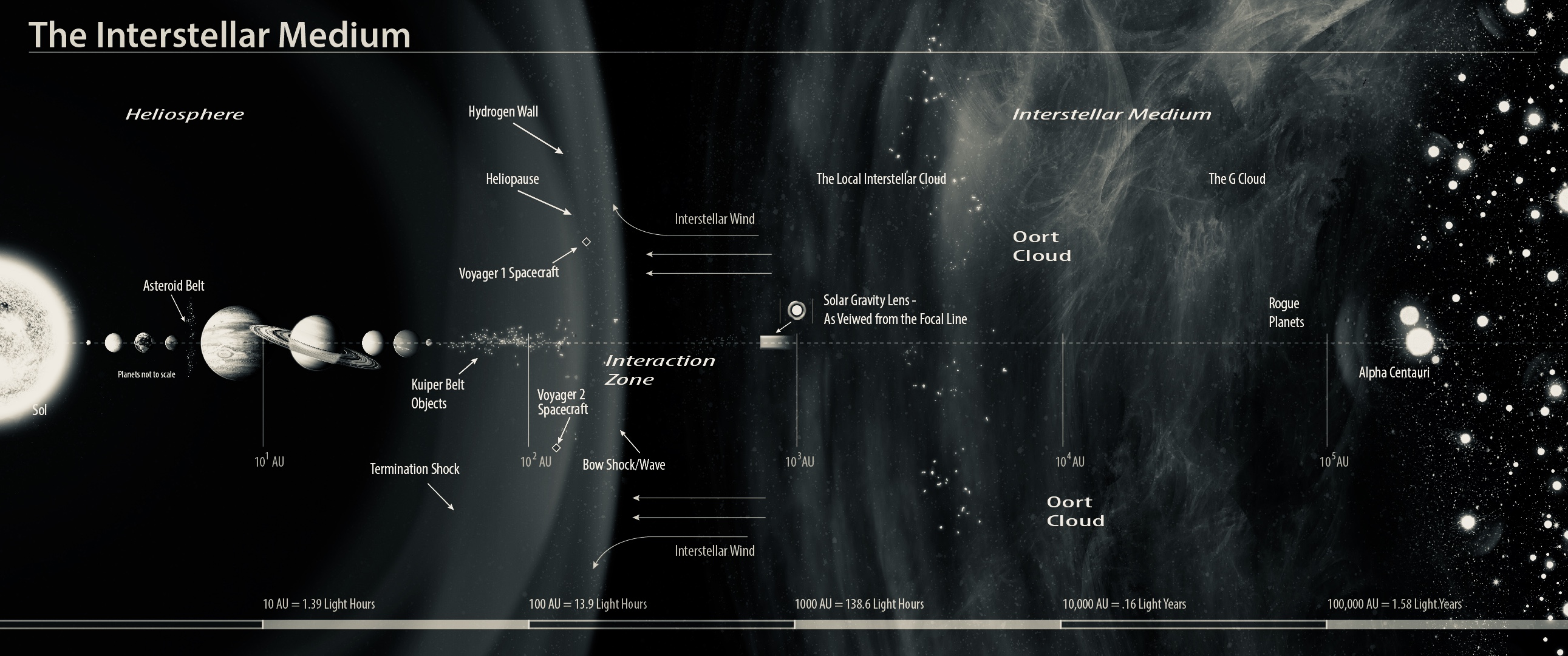
A second problem with detecting the VLF counterpart electromagnetic radiation is that there are various cutoff frequencies due to the plasma in space. In the illustration and table below we give the plasma cutoffs for a detector located in one of three locations: on the Earth, in space but near Earth’s orbit, and finally in interstellar space as shown in Fig. (4).

Region	Observable frequency range
On Earth	$>10$ MHz
Interplanetary space (near Earth’s orbit)	$>$ $20~{}\rm{kHz}-30~{}\rm{kHz}$
Interstellar space (outside the heliosphere)	$>2$ kHz

Figure 4: Log scale illustration of the regions of space within our solar system and galaxy UCSB and the associated plasma frequency cutoff in each region Jones17 ; Lacki10 .

For a detector on Earth one can detect electromagnetic radiation with a frequency of $10~{}\rm{MHz}$ or larger. Assuming this electromagnetic wave came from production by a gravitational wave, this would require a gravitational wave frequency of $5~{}\rm{MHz}$. Since non-exotic gravitational waves sources are expected to have frequencies that are orders of magnitude lower than this, this rules out an Earth based detector for such VLF electromagnetic radiation.

For a detector at the outer edge of the Solar System, near interstellar space, one has a plasma cutoff of $2~{}\rm{kHz}$ which would require a gravitational wave frequency of $1~{}\rm{kHz}$. The fundamental (i.e. f-modes) of neutron star quakes have frequencies in the range $1-3~{}\rm{kHz}$ Kokkotas97 and thus upon doubling this frequency could produce counterpart VLF electromagnetic radiation above the $2~{}\rm{kHz}$ cutoff. In fact the Voyager probes did detect such VLF electromagnetic radiation Kurth84 in the range of $2-3~{}\rm{kHz}$ showing that detection of such VLF electromagnetic radiation is possible Thus one could detect counterpart VLF electromagnetic radiation from the $f$-modes of neutron star quakes if the neutron star were close enough. However, it requires sending a probes to the edge of the Solar System or beyond.

Given that sending probes to the edge of the Solar System is costly both in terms of time and money one could ask if there are gravitational wave sources which would give rise to VLF electromagnetic radiation, which could be detected near Earth’s orbit. From Fig. (4) one can see that for detection one needs the electromagnetic radiation to have a frequency greater than $20-30$ kHz. This implies that the gravitational wave vacuum producing the electromagnetic radiation would need to have a frequency in the range $10-15$ kHz. Theoretical models show that of gravitational wave of this kHz frequency range could be produced from neutron star oscillations Kokkotas97 ; Kokkotas01 . There are different types of neutron star oscillation modes. Three of the most common are: (i) p-modes or “pressure modes” Kokkotas97 with a frequency range $5-9~{}\rm{kHz}$; (ii) f-modes or “fundamental modes” Kokkotas97 with a frequency range of $1-3~{}\rm{kHz}$; (iii) w-modes or “space-time modes” Anderson96 with a frequency range of $8-16~{}\rm{kHz}$ or greater. From this list of oscillation modes the w-modes have the most promising frequency range in terms of detection of the counterpart VLF electromagnetic radiation.

We now want to give a rough estimate of the strength of the electromagnetic flux produced by gravitational waves coming from a w-mode oscillation of a neutron star quake. First from abadie the gravitational wave amplitude at Earth for f-mode generated gravitational waves from a neutron star that is $1$ kpc or $3\times 10^{19}$ m distant from Earth would be of order $h_{+}\sim 10^{-23}$. The associated w-modes gravitational wave amplitude is expected to be down from this by at least one order of magnitude $h_{+}\sim 10^{-24}$. Using this w-mode amplitude and the $1/r$ fall off relation

$$h_{+}=10^{-24}\frac{1~{}{\rm kpc}}{r}$$ (67)

we can determine the amplitude at some point close to the source. For this we take $r^{(0)}=3\times 10^{4}$ m Jones17 – this is far enough from the neutron star that the plane wave approximation we have used throughout should apply, at least roughly. Using (67) and $r^{(0)}=3\times 10^{4}$ m we find that the w-mode amplitude near the source would be of order $h_{+}^{(0)}\sim 10^{-9}$. Using this amplitude, a frequency of 10 kHz in the w-mode range $8-16$ kHz, we can determine the flux of the gravitational wave near the source (i.e. at $r^{(0)}=3\times 10^{4}$ m) using the formula Schutz96

$$F^{(0)}_{gw}=\frac{c^{3}}{16\pi G}|{\dot{\epsilon}}|^{2}=\left(3\times 10^{35}\frac{Ws^{2}}{m^{2}}\right)h_{+}^{2}f^{2}=3\times 10^{25}\frac{W}{m^{2}}~{},$$ (68)

where $\epsilon=h_{+}e^{iku}$ as defined below equation (20). We can now calculate the flux of the counterpart VLF electromagnetic radiation using (68) in (53) to give

$$F^{(0)}_{em}=2\times(10^{-9})^{2}\times(3\times 10^{25}\frac{W}{m^{2}})=6.0\times 10^{7}\frac{W}{m^{2}}~{}.$$ (69)

From (68) and (69) we find that $F^{(0)}_{gw}\gg F^{(0)}_{em}$ which is expected – the electromagnetic radiation produced is much smaller than the gravitational wave which produced it. However, $F^{(0)}_{em}$ is nevertheless large enough that even taking into account the $1/r$ fall off one could potentially detect this electromagnetic radiation at the location of the Earth’s orbit. Taking the flux $F^{(0)}_{em}$ from (69) one can determine the flux at the location of the Earth assuming that the neutron star is 1 kpc away.

$$F_{em}=F^{(0)}_{em}\left(\frac{r^{(0)}}{1kpc}\right)\sim 6.0\times 10^{-23}\frac{W}{m^{2}}~{},$$ (70)

where $r^{(0)}=3\times 10^{4}$ m from before. A flux of the magnitude in (70) could be detected Jones17 and given the frequency range of the w-modes the associated VLF electromagnetic radiation would have a frequency that is above the plasma cutoff at the location of Earth’s orbit as given in Fig. (4). Thus the proposal to detect such the hypothesized co-produced VLF electromagnetic radiation, coming w-modes of neutron star quakes, would be to place a satellite capable of detecting such radiation near earth’s orbit Jones17 ; Gretarsson18 . The old Explorer 49 satellite was capable of detecting such VLF electromagnetic radiation. The Explorer 49 satellite was a Lunar orbiting satellite which was periodically occulted by the Moon in order to block out interference from Solar emissions. The occultation allows one to detect weak signals like (70) above the interference from the Sun.

VII Conclusion and Future prospects

For over 100 years there was nothing to support Faraday’s expectation of a relationship between gravity and electromagnetism. However, in the past 50 years we have seen the development of considerable theoretical support for this relationship and in particular the relation between gravitational and electromagnetic radiation. The earliest work was by Gertsenshtein Gertsenshtein60 demonstrating that electromagnetic radiation can produce gravitational radiation. This was followed in 1975 by Skobelev Skobelev75 who calculated the small but non-zero amplitudes for the $graviton+graviton\to photon+photon$ processes. Beginning around the same time as reference Skobelev75 , there was work that examined the production of electromagnetic fields/multiple photons from a gravitational background unruh-det ; dewitt-det ; hawking ; unruh ; Jones15 . Rrcently we have worked on calculations of the production of electromagnetic radiation by gravitational waves propagating in vacuum Jones16 ; Jones17 ; Jones18 . Perhaps in the next 50 years we will see empirical evidence of the relation between gravitational and electromagnetic radiation by either direct or indirect observation.

The most promising possibility for direct observation is the detection of VLF counterpart production by gravitational waves from neutron star quakes Jones17 . This would only be possible using space based detectors such as the Voyager missions Kurth84 ; Kurth03 ; Webber09 or with a lunar occulted detector similar to the Explorer 49 mission Gretarsson18 . However, detection of counterpart production locally would be limited to the highest frequencies of the counterpart production from neutron star gravitational waves. Detectors in the outer heliosphere would be much more effective and rather remarkably the Voyager space craft are still making observations in the $2-4~{}\rm{kHz}$ range of expected counterpart production Gurnett15 .

Even without direct observation it is possible that the counterpart production of electromagnetic radiation would have important applications in astrophysical processes. One intriguing possibility is in the energetics of core collapse supernovae. The prompt production of gravitational waves from the core collapse would produce gravitational waves with quadruple amplitudes on the order of $1~{}\rm{m}$ and strain amplitude of something like $10^{-5}-10^{-4}$ in the star layers just outside the core. These strain amplitudes have the potential of producing counterpart radiation of sufficient energy to contribute to the energetics of the supernovae. Previous work on fully general relativistic magnetohydrodynamics Font07 (MHD) have assumed the “ideal” MHD condition. This assumption suppresses any potential production of electromagnetic radiation from the strong gravitational wave background. More recent work Obergaulinger14 ; Just18 ; Obergaulinger18 on the effects of magnetic fields and rotation on the energetics of core collapse supernovae have not been fully general relativistic and again could not include the energy from production of electromagnetic radiation by the outgoing gravitational wave. Fully general relativistic MHD simulations have been implemented Lehner12_86 for collapsing hyper-massive neutron stars but not for the study of core collapse supernovae. It is possible that the energy associated with electromagnetic production by gravitational waves outside the iron core could contribute importantly to the supernova, but only fully general relativistic MHD simulations would account for this phenomena in the processes of core collapse and explosion.

Since the production of electromagnetic radiation by gravitational waves is so fundamental it is likely that further study of this phenomena could illuminate our understanding of nature. One recent example of the potential importance of production of photons in a gravitational wave background is the investigation of graviton-photon oscillations in alternatives to general relativity Cembranos18 ; ejlli . This investigation did not directly study counterpart production and potential general relativity violations but does describe the significance of this phenomena in investigating theories of gravity. Counterpart production by gravitational waves Ricciardone17 could also be important in studies of cosmology. Following the Planck epoch the Standard Model fields were still massless for some time. It would be interesting to consider the production of the massless Standard Model particles by primordial gravitational waves during the grand unification epoch and prior to the Standard Model particles acquiring mass via the Higgs mechanism.

References

- (1) Gerald James Holton, Thematic origins of scientific thought: Kepler to Einstein (Cambridge, MA, 1988) 53-74. https://dash.harvard.edu/handle/1/23975383
- (2) Michael Faraday, Experimental researches in electricity, Vol 3 (Dover publications inc., New York, 1965) 161-168.
- (3) V. V. Skobelev, Soviet Physics Journal, 18, 62-65 (1975).
- (4) G.W. Gibbons, Commun. Math. Phys. 45, 191 (1975).
- (5) G. Modanese, Phys. Lett. B 348, 51-54 (1995).
- (6) G. Fiore and G. Modanese, Nucl. Phys. B 477, 623-651 (1996).
- (7) Preston Jones and Douglas Singleton, Int. J. Mod. Phys. D 24 12, 1544017 (2015).
- (8) Preston Jones, Patrick McDougall, and Douglas Singleton, Phys. Rev. D 95, 065010 (2017).
- (9) Preston Jones, Andri Gretarsson, and Douglas Singleton, Phys. Rev. D 96, 124030 (2017).
- (10) Preston Jones, Patrick McDougall, Michael Ragsdale, and Douglas Singleton, Physics Letters B 781, 621-625 (2018).
- (11) Andri Gretarsson, Preston Jones, and Douglas Singleton, “Gravity’s light in the shadow of the Moon”, arXiv:1805.06788.
- (12) P. C. W. Davies, CHAOS 11, 539-547 (2001).
- (13) James Clerk Maxwell, A treatise on electricity and magnetism, Vol 2 (Dover publications inc., New York, 1954) 439.
- (14) Ezra Newman and Roger Penrose, J. Math. Phys. 3, 566-578 (1962).
- (15) Saul A. Teukolsky, The Astrophysical Journal 185, 635-647 (1973).
- (16) G. F. R. Ellis, Cargese Lectures in Physics (Gordon and Breach, New York, 1973) ed. Evry Schatzman, 1-60.
- (17) Sebastiano Sonego and Marek A. Abramowicz, Journal of Mathematical Physics, 39, 3158 (1998).
- (18) P. A. Hogan and S. O’Farrell, Phys. Rev. D 79, 104028 (2009).
- (19) Carlos Palenzuela, Travis Garret, and Steven Liebling, Phys. Rev. D 82, 044045 (2010).
- (20) Philipp Mösta, Carlos Palenzuela, Lucianno Rezzello, Luis Lehner, Shin’ichirou Yoshida and Denis Pollney, Phys. Rev. D 81, 064017 (2010).
- (21) Miguel Zilhão, Vitor Cardoso, Carlos Herdeiro, Luis Lehner, and Ulrich Sperhake, Phys. Rev. D 85, 124062 (2012).
- (22) Luis Lehner, Carlos Palenzuela, Steven L. Liebling, Christopher Thompson, and Chad Hanna, Phys. Rev. D 86, 104035 (2012).
- (23) Luis Lehner, Steven L. Liebling, Carlos Palenzuela, and Patrick M. Motl, Phys. Rev. D 94, 043003 (2016).
- (24) Walter Greiner, Joachim Reinhardt, Field quantization, (Springer-Verlag, Berlin Heidleberg 1996) 154.
- (25) Christos G. Tsagas, Class. Quant. Grav. 22, 393- 408 (2005).
- (26) Bernard F. Schutz, “Gravitational Radiation”, Encyclopedia of Astronomy and Astrophysics (Institute of Physics Publishing, Bristol, and Macmillan Publishers Ltd, London, 2000), arXiv:gr-qc/0003069v1.
- (27) Jorge L. Cervantes-Cota, Salvador Galindo-Uribarri, George F. Smoot, Universe, 2 22 (2016).
- (28) Bernard F. Schutz, A first course in general relativity, 2nd edition, (Cambridge University Press, Cambridge 2009) 210-212.
- (29) B. S. Sathyaprakash and Bernard F. Schutz, “Physics, Astrophysics and Cosmology with Gravitational Waves”, Living Reviews of Relativity 12 2 (2009).
- (30) B. P. Abbott et al. (LIGO Scientific Collaboration and Virgo Collaboration) Phys. Rev. Lett. 116, 061102 (2016); ibid. Phys. Rev. Lett. 116, 241103 (2016); ibid. Phys. Rev. Lett. 118, 221101 (2017).
- (31) Abbott et al., “Multi-messenger observation of a binary neutron star merger”, Astrophysical Journal, 848, L12 (2017). LIGO.
- (32) M. E. Gertsenshtein, Soviet Physics JETP, 14 1, 84-85 (1960).
- (33) G. A. Lupanov, J. Expt. Theo. Phys. 52, 118 (1967).
- (34) C, Sabin, D. E. Bruschi, M. Ahmadi, and I. Fuentes, New J. Phys. 16, 085003 (2014).
- (35) N. E. J. Bjerrum-Bohr, Barry R. Holstein, Ludovic Plant, Pierre Vanhove, “Graviton-Photon Scattering”, arXiv:1410.4148v2.
- (36) L. Parker, Phys. Rev. Lett. 21, 562 (1968).
- (37) L. Parker, Phys. Rev. 183, 1057 (1969).
- (38) L. Parker, Phys.Rev. D 3, 346 (1971), Erratum: Phys.Rev. D 3, 2546 (1971).
- (39) S. Deser, J. Phys. A 8, 1972 (1975).
- (40) J. Garriga and E. Verdaguer, Phys. Rev. D 43, 391 (1991).
- (41) N. D. Birrell and P. C. W. Davies, Quantum Fields in Curved Space (Cambridge University Press, Cambridge, England, 1982).
- (42) C. Stahl, E. Strobel, and S.-S. Xue, Phys. Rev. D 93, 025004 (2016); C. Stahl and S.-S. Xue, Phys. Lett. B 760, 288 (2016).
- (43) F. Halzen and A. D. Martin, Quarks and Leptons: An Introductory Course in Modern Particle Physics (John Wiley & Sons, New York, 1984).
- (44) W. G. Unruh Particle detectors and black holes, Proceedings of the First Marcel Grossmann Meeting on General Relativity, ed. by R. Ruffini, North-Holland (Amsterdam, 1977) pp. 527- 536.
- (45) B. S. DeWitt (1979) Quantum gravity: The new synthesis, General Relativity: An Einstein Centenary Survey, ed. by S. W. Hawking and W. Israel, Cambridge University Press (Cambridge, 1979). pp. 680-745.
- (46) S. W. Hawking, Commun. Math. Phys. 43, 199 (1975) [Erratum-ibid. 46, 206 (1976)].
- (47) W. G. Unruh, Phys. Rev. D 14, 870 (2001).
- (48) J. R. Letaw and J. D. Pfautseh, Phys. Rev. D 22, 1345 (1980); J. R. Letaw, Phys.Rev. D 23, 1709 (1981).
- (49) E. T. Akhmedov and D. Singleton, Int. J. Mod. Phys. A 22 (2007) 4797.
- (50) D. Singleton and S. Wilburn, Phys. Rev. Lett. 107, 081102 (2011) 081102.
- (51) N. Rad and D. Singleton, Eur. Phys. J. D 66, 258 (2012).
- (52) E. Bertschinger and E. F. Taylor “Chapter 16, Gravitational Waves” (2014), available at http://www.eftaylor.com/exploringblackholes/Ch16GravWaves171018v1.pdf.
- (53) M. Hendry, “An Introduction to General Relativity, Gravitational Waves and Detection Principles”, Second VESF School on Gravitational Waves, Cascina, Italy, May 28th–June 1st, 2007, http://star-www.st-and.ac.uk/∼hz4/grhendry GRwaves.pdf
- (54) D. Griffiths, Introduction to Elementary Particles, 2nd edn. (Wiley-VCH, Weinheim, 2008), p. 313.
- (55) X. Calmet, I. Kuntz and S. Mohapatra, Eur. Phys. J. C 76, 425 (2016).
- (56) H. Nikolić, Phys. Lett. B 527, 119 (2002); 529, 265(E) (2002).
- (57) M. B. Fröb, J. Garriga, S. Kanno, M. Sasaki, J. Soda, T. Tanakac, and A. Vilenkin, J. Cosmol. Astropart. Phys. 04, 009 (2014).
- (58) UCSB experimental cosmology group, http://www.deepspace.ucsb.edu/directed-energy-interstellar-precursors.
- (59) Brian C. Lacki, Mon. Not. R. Astron. Soc. 406, 863-880 (2010).
- (60) Kotas D. Kokkotas, “Stellar pulsations and gravitational waves”, Mathematics of gravitation, part 2, gravitational wave detection, Banach center publications, vol. 41, Institute of Mathematics, Polish Academy of Sciences, 31-41 (1997).
- (61) W. S. Kurth, D. A. Gurnett, F. L. Scarf, and R. L. Poynter, Nature 312, 27-31 (1984).
- (62) D. A. Gurnett, W. S. Kurth, and E. C. Stone, Geophysical Research Letters 30 23, 2009 (2003).
- (63) W. R. Webber and D. S. Intriligator, arxiv:0906:2746 (2009).
- (64) Kostas D. Kokkotas and Nils Anderson, SIGRAV XIV, Genoa 2000 (Springer-Verlg 2001), arXiv:gr-qc/0109054.
- (65) Nils Anderson, Kostas D. Kokkotas, and Bernard F. Schutz, Mon. Not. R. Astron. Soc. 280, 1230-1234 (1996).
- (66) J. Abadie et al., Phys. Rev. D 83, 042001 (2011).
- (67) B. F. Schutz, Class. Quantum Grav., 13, A219- A238 (1996).
- (68) D. A. Gurnett, W. S. Kurth, E. C. Stone, A. C. Cummings, S. M. Krimigis, R. B. Decker, N. F. Ness, and L. F. Burlag, Astrophys. J. 809 121 (2015).
- (69) José A. Font, J. Phys.: Conf. Ser. 66 012063 (2007).
- (70) Martin Obergaulinger, Hans-Thomas Janka, Miguel-Ángel Aloy, MNRAS 445 3169–3199 (2018).
- (71) Oliver Just, Robert Bollig, Hans-Thomas Janka, Martin Obergaulinger, Robert Glas, Shigehiro Nagataki, MNRAS 481 4786–4814 (2018).
- (72) Martin Obergaulinger, Oliver Just, and Miguel-Ángel Aloy, J. Phys. G: Nucl. Part. Phys. 45 084001 (2018).
- (73) José A. R. Cembranos, Marío Coma Díaz, Prado Martin-Moruno, Class. Quantum Grav. 35 205008 (2018).
- (74) D. Ejlli and V. R. Thandlam, “GRAPH mixing” arXiv:1807.00171 [gr-qc]
- (75) Angelo Ricciardone, J. Phys.: Conf. Ser. 840 012030 (2017).