Grid-based diffusion Monte Carlo for fermions without the fixed-node approximation

Abstract

A diffusion Monte Carlo algorithm is introduced that can determine the correct nodal structure of the wave function of a few-fermion system and its ground-state energy without an uncontrolled bias. This is achieved by confining signed random walkers to the points of a uniform infinite spatial grid, allowing them to meet and annihilate one another to establish the nodal structure without the fixed-node approximation. An imaginary-time propagator is derived rigorously from a discretized Hamiltonian, governing a non-Gaussian, sign-flipping, branching, and mutually annihilating random walk of particles. The accuracy of the resulting stochastic representations of a fermion wave function is limited only by the grid and imaginary-time resolutions and can be improved in a controlled manner. The method is tested for a series of model problems including fermions in a harmonic trap as well as the He atom in its singlet or triplet ground state. For the latter case, the energies approach from above with increasing grid resolution and converge within $0.015~{}{E}_{\text{h}}$ of the exact basis-set-limit value with a statistical uncertainty of $10^{-5}~{}{E}_{\text{h}}$ without an importance sampling or Jastrow factor.

I Introduction

Stochastic algorithms Kalos (1962); Anderson (1975); Lüchow (2011) hold exceptional promise in treating correlated electronic structures owing to their high parallel efficiency, near-exact accuracy, scalability with the problem size, and tiny memory footprints. Perhaps, the most successful of such algorithms is diffusion Monte Carlo (DMC) Anderson (1975), but it is notoriously plagued by an uncontrolled bias (the fixed-node error) arising from the fixed-node approximation Klein and Pickett (1976); P. J. Reynolds et al. (1982); Anderson (1975) introduced as a practical solution to the sign problem Troyer and Wiese (2005). It amounts to using the nodal structure of some trial wave function, which differs from the exact one, thus causing the error.

The objective of this work is to eliminate the fixed-node error from DMC Anderson (1975). This is achieved by confining the positively and negatively signed walkers on an infinite, uniform, real-space grid, which can thus meet on a grid point and then annihilate one another, establishing a nodal structure without the fixed-node or any other similar approximation. The resulting nodal structure should converge at the exact one in the limit of infinitesimally small grid spacing and imaginary time step. A general stochastic propagation protocol on a grid is derived in this work. Our method—grid DMC—is distinguished from any of the previously developed fermion quantum Monte Carlo approaches that enforce annihilation by walker pairing, correlated dynamics, or other techniques Carlson and Kalos (1985); Coker and Watts (1986); J. B. Anderson et al. (1991); Kalos (1996); Kalos and Schmidt (1997); Kalos and Pederiva (2000); Mishchenko (2006).

Casula et al. M. Casula et al. (2005); Casula et al. (2010) were among the first to introduce a real-space grid in DMC, but for the different purpose of implementing a nonlocal pseudopotential. Like their method, our grid DMC relies on a finite-difference approximation to the kinetic-energy operator on a grid. It also shares some algorithmic features with full-configuration-interaction quantum Monte Carlo (FCIQMC), which propagates signed walkers in a discretized space of the Slater determinants, the latter ensuring the fermion antisymmetry of the wave function. Grid DMC obeys a similar population dynamics as FCIQMC, which is an interplay between propagation, branching, and annihilation of walkers Spencer et al. (2012). A correct nodal structure emerges as the total number of walkers exceeds a critical value, $N_{\text{c}}$, which is a function of the grid spacing, dimension of the configuration space, and character of the target state. The value of $N_{\text{c}}$ determines the memory footprint, which is expected to grow exponentially with the system size as a manifestation of the sign problem Troyer and Wiese (2005).

Clearly, grid DMC is severely limited in its applicability because of the exponential size-dependence of $N_{\text{c}}$, if one insists on solving the Schrödinger equation essentially exactly. In this work, we establish its feasibility just for two-particle (Coulomb) systems in the 3-D space with a view to ultimately realizing DMC-like stochastic algorithms for two-electron theories such as second-order Møller–Plesset perturbation (MP2) Sinanoǧlu (1962); Bischoff and Valeev (2013); Hirata et al. (2017) or coupled-cluster doubles (CCD) theory Kottmann and Bischoff (2017). It may be argued that stochastic MP2 and CCD are expected to be more scalable than their deterministic counterparts (with respect to both the number of processors and problem size) and thus applicable to large systems that do not lend themselves to local-correlation speedup.

This article is structured as follows: A detailed description of our grid-DMC algorithm is given in Sec. II. The results of demonstrative calculations on fermions in a harmonic trap and the He atom in the triplet or singlet ground state are reported in Secs. III.1 and III.2, respectively. A summary of the method and an outline of the future work are given in Sec. IV. In Appendices A and B, mathematical details of the algorithm are given.

II Theory and Algorithms

Let $\Psi(\bm{r}_{1},\dots,\bm{r}_{N},\tau)$ be the wave function of an $N$-particle system satisfying the imaginary-time-dependent Schrödinger equation with energy offset $\omega$,

$$-\frac{\partial\Psi(\bm{r}_{1},\dots,\bm{r}_{N},\tau)}{\partial\tau}=\left(\hat{H}-\omega\right)\Psi(\bm{r}_{1},\dots,\bm{r}_{N},\tau),$$ (1)

where $\hat{H}$ is the Hamiltonian with a local, spin-independent potential $V(\bm{r}_{1},\dots,\bm{r}_{N})$,

$$\hat{H}=-\frac{1}{2}\sum_{i=1}^{N}\nabla_{i}^{2}+V(\bm{r}_{1},\dots,\bm{r}_{N}).$$ (2)

The transition probability of the particles hopping from $(\bm{r}_{1},\dots,\bm{r}_{N})$ to $(\bm{r}_{1}^{\prime},\dots,\bm{r}_{N}^{\prime})$ in short time $\tau$ is approximated by the following Green’s function, using the Suzuki–Trotter expansion Trotter (1959):

$$G(\bm{r}_{1},\dots,\bm{r}_{N}\to\bm{r}_{1}^{\prime},\dots,\bm{r}_{N}^{\prime};\tau)$$

$$\approx\langle\bm{r}_{1}^{\prime},\dots,\bm{r}_{N}^{\prime}|\exp\{-\tau(V-\omega)/{2}\}|\bm{r}_{1}^{\prime},\dots,\bm{r}_{N}^{\prime}\rangle$$

$$\times\,\langle\bm{r}_{1}^{\prime},\dots,\bm{r}_{N}^{\prime}|\sum_{i=1}^{N}\exp(\tau\nabla_{i}^{2}/2)|\bm{r}_{1},\dots,\bm{r}_{N}\rangle$$

$$\times\,\langle\bm{r}_{1},\dots,\bm{r}_{N}|\exp\{-\tau(V-\omega)/2\}|\bm{r}_{1},\dots,\bm{r}_{N}\rangle$$ (3)

$$=\exp\left\{-\tau\left(\frac{V(\{\bm{r}^{\prime}_{i}\})+V(\{\bm{r}_{i}\})}{2}-\omega\right)\right\}$$

$$\times\,\prod_{i=1}^{N}\langle\bm{r}_{i}^{\prime}|\exp(\tau\nabla_{i}^{2}/2)|\bm{r}_{i}\rangle,$$ (4)

where $|\bm{r}_{1},\dots,\bm{r}_{N}\rangle$ and $|\bm{r}_{i}\rangle$ are the position eigenfunctions.

In this work, a particle is confined to a point in an infinite, uniform, 3-D grid with grid spacing $\delta$. The Laplacian in the kinetic-energy operator is approximated by a central three-point finite-difference formula. In this ansatz, each factor in the kinetic-energy part of the Green’s function, Eq. (4), simplifies to

$$\langle\bm{r}^{\prime}|\exp(\tau\nabla^{2}/2)|\bm{r}\rangle$$

$$\approx\langle x^{\prime},y^{\prime},z^{\prime}|\exp(\tau\nabla^{2}/2)|x,y,z\rangle$$ (5)

$$=\langle x+n_{x}\delta,y+n_{y}\delta,z+n_{z}\delta|\exp(\tau\nabla^{2}/2)|x,y,z\rangle$$ (6)

$$=p_{n_{x}}p_{n_{y}}p_{n_{z}}$$ (7)

with

$$p_{n} = \left\langle x+n\delta\left|\exp\left(\frac{\tau}{2}\frac{\partial^{2}}{\partial x^{2}}\right)\right|x\right\rangle$$ (8)

$$= \frac{1}{2\pi}\int_{-\pi}^{\pi}\cos(kn)\exp\left\{-\frac{2\tau}{\delta^{2}}\sin^{2}\left(\frac{k}{2}\right)\right\}dk,$$ (9)

where it should be understood that $(x,y,z)$ and $(x^{\prime},y^{\prime},z^{\prime})$ are grid points and $n_{x}$, $n_{y}$, and $n_{z}$ are integer displacements. For the derivation of Eq. (9), see Appendix A.

Evidently, $p_{n}$ is the non-Gaussian transition probability of a particle hopping from a grid point to its $n$th nearest neighbor (where $n$ is a positive or negative integer) in an infinite, evenly-spaced, 1-D grid. It satisfies the following properties expected of such probability:

$$p_{n} = \delta_{n0}\,\,\text{for }\tau=0,$$ (10)

$$p_{n} \geq 0,$$ (11)

and

$$\sum_{n=-\infty}^{\infty}p_{n} = 1.$$ (12)

The proofs of these identities can be found in Appendix B.

Equation (II) contains moves essentially corresponding to an interchange of particles with the same spin, which should, therefore, reverse its sign when applicable. This can be encoded by introducing a canonical order of the grid points and associating the Green’s function with the parity of the permutation that brings the sequence of the destination grid points into a canonical order. In this work, we define a canonical order as one with the increasing $x$ coordinates first, then with the increasing $y$ coordinates, and finally with the increasing $z$ coordinates. Examples of sign-preserving and sign-flipping moves are depicted in Fig. 1 for a simple case of two same-spin fermions on a 2-D grid.

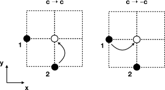
Figure 1: Examples of sign-preserving (left) and sign-flipping (right) moves for two fermions (labeled ‘1’ and ‘2’) with the same spin on a 2-D grid. The grid points are canonical ordered in the increasing $x$ coordinates first, and then in the increasing $y$ coordinates. In the move shown on the left, the coordinates of particles 1 and 2 are in a canonical order before and after the move, preserving the sign of $c$. The move shown on the right brings the coordinates of particles 1 and 2 into a non-canonical order, which needs to be permuted once to be canonical-ordered, causing a sign flip in $c$.

The foregoing equations admit a stochastic implementation similar to DMC Anderson (1975); Lüchow (2011) with a major difference being in the definition of random walkers and their (signed) transition probabilities. Each walker represents a set of all particles, carrying a unit signed weight, $c=\pm 1$. The $i$th particle has spatial coordinates that are on a point in an infinite, uniform grid with a grid spacing of $\delta$ and spin label $s_{i}=\pm 1/2$ (in the case of an electron) so that $\sum_{i=1}^{N}s_{i}=S_{z}$, where $S_{z}$ is the total magnetic spin angular momentum quantum number of the target state. The walker weight $c$ flips sign, whenever an odd number of permutations is needed to bring the particle coordinates into a canonical order after a move. The calculation workflow is similar to that of DMC and consists of the following steps:

1. Initialization. An initial walker population is randomly generated from some real trial wave function $|\Psi_{\text{T}}(\bm{r}_{1},\dots,\bm{r}_{N})|$ (which must not be confused with a trial wave function in the fixed-node approximation) by the Metropolis algorithm Metropolis et al. (1953), exercising care to avoid Coulomb singularities. The initial walker weights are assigned with the sign of $\Psi_{\text{T}}$. Factors $p_{n}$ of Eq. (9) are computed as a function of $n$ by numerical integration and stored.

2. Propagation. Each walker performs a random walk. This step is executed by looping over all particles $(i=1,\dots,N)$ and displacing the grid coordinates of each particle relatively by $(n_{x},n_{y},n_{z})$ with a transition probability of $p_{n_{x}}p_{n_{y}}p_{n_{z}}$. The walker weight $c=\pm 1$ is then multiplied by $(-1)^{[P]}$, where $[P]$ is the parity of permutation $P$ that brings the sequence of the new particle coordinates into a canonical order.

3. Branching. For each walker, the old $(\bm{r}_{1},\dots,\bm{r}_{N})$ and new $(\bm{r}^{\prime}_{1},\dots,\bm{r}^{\prime}_{N})$ sets of the particle coordinates are used to calculate the branching factor, $m=\exp[-\tau\{(V(\{\bm{r}^{\prime}_{i}\})+V(\{\bm{r}\}))/2-\omega\}]$. The walker is subsequently replaced by $\lfloor m+\xi\rfloor$ copies, where $\xi$ is a random number sampled from a uniform distribution on the interval $[0,1]$.

4. Annihilation. The list of all walkers is sorted and then searched for the members whose particles occupy the identical set of grid points. An equal number of positively and negatively signed walkers among them are annihilated, leaving only a minimal number of like-signed walkers on each set of grid points.

5. Energy estimation. The energy offset $\omega$ is updated as $\omega\rightarrow\omega+\tau^{-1}\ln(N_{\text{w}}/N_{\text{w}}^{\prime})$ to keep the number of walkers approximately constant, where $N_{\text{w}}$ and $N_{\text{w}}^{\prime}$ are the sizes of the old and new walker lists, respectively. The mean value of $\omega$ in the limit $\tau\to\infty$ can be used to estimate the ground-state energy,

   $$E_{\text{gr}}=\langle\omega\rangle,$$ (13)

   which is known as the growth estimator C. J. Umrigar et al. (1993). A more desirable measure of energy according to statistical uncertainty considerations is the projection estimator An and van Leeuwen (1991); G. H. Booth et al. (2009) defined as follows:

   $$E_{\text{proj}}=\left\langle\frac{\sum_{k}c_{k}\hat{H}\Psi_{\text{T}}(\bm{r}^{[k]}_{1},\dots,\bm{r}^{[k]}_{N})}{\sum_{k}c_{k}\Psi_{\text{T}}(\bm{r}^{[k]}_{1},\dots,\bm{r}^{[k]}_{N})}\right\rangle$$ (14)

   at $\tau\to\infty$, where $c_{k}$ and ($\bm{r}^{[k]}_{1},\dots,\bm{r}^{[k]}_{N}$) are the weight and grid points of the $k$th walker, and $\Psi_{\text{T}}$ is any trial wave function (which may differ from the one used in Step 1) having a non-zero overlap with the exact wave function.

Steps 2 through 5 are repeated (with each cycle counted as one Monte Carlo step) until convergence. For a sufficiently large number of walkers, $N_{\text{w}}$, the computational cost of a Monte Carlo cycle is dominated by the annihilation step, which exhibits $N_{\text{w}}\ln N_{\text{w}}$ scaling of computational complexity owing to the need to sort the walker list. As will be shown in the next section, another important implication of the annihilation is the existence of the critical number of walkers, $N_{\text{c}}$, required to obtain the correct nodal structure, which grows exponentially with the dimension of the configuration space. The value of $N_{\text{c}}$ defines the memory footprint and limits the application size. The lack of annihilation for a small number of walkers, i.e., $N_{\text{w}}<N_{\text{c}}$, leads to node sampling errors and introduces a nodal bias in the energy estimates G. H. Booth et al. (2009).

III Results and Discussion

A Python program of grid DMC was written and made available online Kunitsa (2019). The transition probabilities $p_{n}$ were calculated (with a maximum error of $10^{-10}$) using the Clenshaw–Curtis adaptive quadrature implemented in the gnu scientific library Galassi . Displacements with the probabilities smaller than $10^{-8}$ were discarded. Statistical errors in the energies were evaluated using the blocking analysis Flyvbjerg and Petersen (1989) as implemented in pyblock module Spencer (2014).

III.1 Fermions in a harmonic trap

Consider a system of four noninteracting spin-1/2 particles with a unit mass confined in a 1-D harmonic trap characterized by a potential, $V=\sum_{i=1}^{4}x_{i}^{2}/2$, where $x_{i}$ is the $i$th particle coordinate. It lends itself to analytical solution of the Schrödinger equation with the exact energy, $E=\sum_{i=1}^{4}(n_{i}+1/2)$ in the units of $E_{\text{h}}$, where $n_{i}$ is the $i$th quantum number of the 1-D harmonic oscillator which is a nonnegative integer. States with the total spin quantum number $S=0$, $1$, and $2$ were studied by grid DMC with a grid spacing of $\delta=0.1$ a.u. and an imaginary time step of $\tau=0.1$ a.u. The initial particle positions were sampled from a uniform distribution on a 6.0-a.u. interval centered at the origin. An ensemble of $\sim 10^{7}$ random walkers was propagated over 5000 Monte Carlo steps. The energy was evaluated by the growth estimator. Table 1 compiles the results.

The $S=0$ ground state has a pair of $\alpha$- and $\beta$-spin particles occupying the $n=0$ one-particle harmonic-oscillator level and another $\alpha\beta$ pair occupying the $n=1$ level, having the exact energy of $4.0~{}E_{\text{h}}$. The $S=1$ ground state has two particles in the $n=0$ level and one $\alpha$-spin particle each in the $n=1$ and $2$ levels, whereas the $S=2$ ground state has one $\alpha$-spin particle each in the $n=0$, $1$, $2$, and $3$ levels. The correct nodal structure of the $n\geq 1$ one-particle wave functions and the overall antisymmetry of the four-particle wave function naturally emerge in these grid-DMC calculations. Unlike DMC with the fixed-node approximation, where the wave function in each nodal packet has the correct shape, but not throughout the whole space even after adjusting the sign of each packet, the wave function obtained in grid DMC has the correct shape in the whole space.

The grid-DMC energies are accurate within $0.006$, $0.01$, and $0.02~{}E_{\text{h}}$ of the exact values of the $S=0$, $1$, and $2$ states, respectively. They are many orders of magnitude greater than the statistical uncertainty of $\sim 5\times 10^{-5}~{}E_{\text{h}}$, and so they are biases. The main sources of the biases are the nonzero grid spacing and finite time step. When the deterministic calculations were performed using the same grid (i.e., the diagonalization of the discretized Hamiltonian on a uniform grid spanning 6 a.u. using the central three-point finite-difference formula with $\delta=0.1$ a.u.), their energies are within $0.002\sim 0.004~{}E_{\text{h}}$ of the grid-DMC results. These remaining biases are attributed to the finite time step.

Table 1: Growth-estimator energies (statistical uncertainties in parentheses) in $E_{\text{h}}$ of the $S=0$, $1$, and $2$ states of the system with four noninteracting spin-1/2 fermions with a mass of 1 a.u. in a 1-D harmonic trap.

$S$	Grid DMC	Grid	Exact
0	$3.99458(4)$	3.99625	4.0
1	$4.99168(4)$	4.99374	5.0
2	$7.98292(5)$	7.98622	8.0

In order to study the efficacy of the walker annihilation, we performed a series of runs with varying walker ensemble sizes. The simulation results are given in Fig. 2. The left panel shows that the energies converge at the correct limits, provided that the annihilation events are sufficiently frequent or, equivalently, the number of walkers exceeds a threshold value $N_{\text{c}}$, which varies with the character of the target state. The lack of a sufficient number of annihilation events causes the underestimation of the energies. The rate of convergence tends to decrease for higher spin states, in which particles occupy one-particle levels with more nodes. The population dynamics presented in the right panel, obtained by holding $\omega$ fixed (a production run adjusts $\omega$), is reminiscent of that obtained in FCIQMC G. H. Booth et al. (2009), similarly exhibiting pronounced plateaus signaling that $N_{\text{w}}$ has reached $N_{\text{c}}$. The plateaus occur because of the competition between the spawning and walker annihilation Spencer et al. (2012).

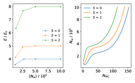
Figure 2: Left: the energy evaluated by the growth estimator, $E$, as a function of the average number of walkers, $\langle N_{\text{w}}\rangle$, for the $S=0$, $1$, and $2$ ground states of the four noninteracting fermions in a 1-D harmonic trap. Right: The number of walkers, $N_{\text{w}}$, as a function of the Monte Carlo steps, $N_{\text{MC}}$. The energy onset, $\omega$, was held fixed at 4.25, 5.25, and 8.25 $E_{\text{h}}$ for the states with $S=0$, $1$, and $2$, respectively.

The dependence of $N_{\text{c}}$ on the grid spacing was further analyzed for two spin-1/2 fermions in a 3-D harmonic trap in the triplet ground state (Fig. 3). Owing to the higher dimension of the configuration space, $N_{\text{c}}$ is orders of magnitude larger than in the 1-D system and exhibits a steep growth with decreasing $\delta$. A least-squares fit suggests that $N_{\text{c}}\approx 339\,\delta^{-5.99}$. In general, one could expect $N_{\text{c}}\propto\delta^{-nd}$, where $n$ is the number of particles and $d$ is the dimension of the configuration space.

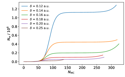
Figure 3: The number of walkers, $N_{\text{w}}$, as a function of the Monte Carlo steps, $N_{\text{MC}}$, in grid DMC for two spin-1/2 fermions in a 3-D harmonic trap in the triplet ground state for several grid spacings $\delta$. The energy onset was held fixed at $\omega=4.5~{}E_{\text{h}}$ and imaginary time step $\tau=0.1$ a.u.

III.2 The He atom in the ${}^{3}S$ and ${}^{1}S$ states

The grid-DMC algorithm for a system with charged particles requires some modifications to avoid the Coulomb singularities. In contrast to continuous DMC, random walks in a discretized space have a nonzero probability of exact particle coalescence, leading to divergent branching factors. To avoid this, we placed the He nucleus at coordinates $(\delta/2,\delta/2,\delta/2)$, where $\delta$ is the grid spacing, and furthermore barred the random walks that result in electron-electron coalescence. Various grid spacings $\delta$ in the range of 0.01 to 0.16 a.u. were tested, while an imaginary time step of 0.005 a.u. was used in all calculations.

For comparison, we also performed grid-DMC calculations for the ${}^{3}S$ state with the fixed-node approximation using the exact nodal structure D. Bressanini and P. J. Reynolds (2005) as well as for the nodeless ${}^{1}S$ ground state Ceperley (1991). The nodal constraint was imposed by killing walkers attempting to acquire a sign inconsistent with that of a trial wave function $\Psi_{\text{T}}$ having the exact nodal structure. Namely, the walker weight $c_{k}$ was set to zero if $c_{k}\Psi_{\text{T}}(\bm{r}_{1}^{[k]},\bm{r}_{2}^{[k]})<0$. With the assistance of the exact nodal structure, grid-DMC calculations with the fixed-node approximation need only 10000 walkers to converge.

The first six rows of Table 2 list the results of grid-DMC calculations with and without the exact nodal constraint using two grid spacings: $\delta=0.16$ or $0.08$ a.u. In both cases, the convergence with respect to the number of walkers was ensured by repeating the calculation with different walker ensemble sizes and checking the stability of the energy estimates. Additionally, the average fraction ($w$) of walkers with the correct sign (i.e., with the same sign as $\Psi_{\text{T}}$) was recorded to quantify the accuracy of the nodal structure. The closer the values of $w$ to100%, the more accurate the nodal structure of the grid-DMC result without the fixed-node approximation.

With a coarse grid of $\delta=0.16$ a.u., convergence is achieved with $3.5$ to $7\times 10^{7}$ walkers (the number identified as $N_{\text{c}}$) with $97.9$ to $98.3$% accurate nodal structure. The corresponding energies ($-2.1269~{}E_{\text{h}}$) have minuscule statistical uncertainties of $10^{-5}~{}E_{\text{h}}$, but suffer from a much greater bias of $1~{}\text{m}E_{\text{h}}$ from the one with the exact nodal constraint ($-2.1278~{}E_{\text{h}}$). This bias is clearly due to an inexact nodal structure and may be called a nodal bias. The grid-DMC result with the exact nodal constraint is too high as compared with the exact energy ($-2.1753~{}E_{\text{h}}$) Pekeris (1959) by $48~{}\text{m}E_{\text{h}}$, which must be ascribed to a combination of nonzero grid spacing and finite time step. As will be shown below, a majority of this bias is due to the grid spacing and may be called a grid bias.

Halving the grid spacing to $\delta=0.08$ a.u. increases $N_{\text{c}}$ by an order of magnitude to $6\times 10^{8}$. The proportion of walkers with the correct sign deteriorates slightly to 96.7 to 96.8% instead of improves. Interestingly, however, the nodal bias in the energies seems to be compressed to $0.5~{}\text{m}E_{\text{h}}$, although this value is obscured by the statistical uncertainty of a similar size in the grid-DMC calculation with the exact nodal constraint. Nevertheless, it may be concluded that grid DMC can achieve 97-98% accurate nodal structure a priori with a submillihartree nodal bias in the energy for two fermions in the 3-D space. Before an extrapolation to $\delta=0$ limit (see below), it achieves the energy ($-2.1613$ to $-2.1617~{}E_{\text{h}}$) of the He atom in the ${}^{3}S$ state within $15~{}\text{m}E_{\text{h}}$ of the exact nonrelativisitc value Pekeris (1959) without the Jastrow factor or importance sampling.

Further halving the grid spacing to $\delta=0.04$ a.u. might elevate the estimated value of $N_{\text{c}}$ to $3.8\times 10^{10}$, approaching a hardware memory limit.

Table 2: Projection-estimator energies, $E$ (statistical uncertainties in parentheses) of the He atom in the ${}^{3}S$ and ${}^{1}S$ states obtained by grid DMC (with an imaginary time step of $0.005$ a.u.) with and without an exact nodal constraint. $\delta$ is the grid spacing, $\langle N_{\text{w}}\rangle$ is the average number of walkers, and $w$ is the proportion of walkers having the correct sign.

State	Method	$\delta~{}/~{}\text{a.u.}$	$\langle N_{\text{w}}\rangle$	$w~{}/~{}\%$	$E~{}/~{}E_{\text{h}}$
${}^{3}S$	Grid DMC	0.16	$3.5\times 10^{7}$	$97.9$	$-2.12695(1)$
${}^{3}S$	Grid DMC	0.16	$7.0\times 10^{7}$	$98.3$	$-2.12687(1)$
${}^{3}S$	Grid DMC (fn)	0.16	$10^{4}$	$100$	$-2.1278(8)$
${}^{3}S$	Grid DMC	0.08	$6.16\times 10^{8}$	$96.7$	$-2.16126(1)$
${}^{3}S$	Grid DMC	0.08	$6.25\times 10^{8}$	$96.8$	$-2.16169(1)$
${}^{3}S$	Grid DMC (fn)	0.08	$10^{4}$	$100$	$-2.1612(15)$
${}^{3}S$	Grid DMC (fn)	0.04	$10^{4}$	$100$	$-2.1698(8)$
${}^{3}S$	Grid DMC (fn)	0.02	$10^{4}$	$100$	$-2.1724(10)$
${}^{3}S$	Grid DMC (fn)	0.01	$10^{4}$	$100$	$-2.1739(7)$
${}^{3}S$	Grid DMC (fn)	0	$10^{4}$	$100$	$-2.1741$
${}^{3}S$	Exact	$\dots$	$\dots$	$\dots$	$-2.1753$
${}^{1}S$	Grid DMC	0.16	$10^{4}$	$100$	$-2.8355(22)$
${}^{1}S$	Grid DMC	0.08	$10^{4}$	$100$	$-2.8867(14)$
${}^{1}S$	Grid DMC	0.04	$10^{4}$	$100$	$-2.8984(14)$
${}^{1}S$	Grid DMC	0.02	$10^{4}$	$100$	$-2.9032(16)$
${}^{1}S$	Grid DMC	0.01	$10^{4}$	$100$	$-2.9029(15)$
${}^{1}S$	Grid DMC	0	$10^{4}$	$100$	$-2.9035$
${}^{1}S$	Exact	$\dots$	$\dots$	$\dots$	$-2.9037$

The remainder of the calculations in Table 2 were performed with the exact nodal constraint for the ${}^{3}S$ and ${}^{1}S$ states with different grid spacings ($\delta$) to estimate a grid bias. Only 10000 walkers were necessary to converge the energies within a few millihartrees. They are plotted as a function of $\delta$ in Fig. 4.

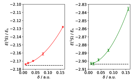
Figure 4: The energies of the He atom in the ${}^{3}S$ (left) and ${}^{1}S$ (right) states obtained by grid DMC with the exact nodal constraint as a function of the grid spacing ($\delta$). Statistical errors are shown with vertical bars. Horizontal dashed lines indicate the exact nonrelativistic energies Pekeris (1959). Quadratic fit of the grid-DMC energies are drawn with solid curves.

For both states, the plots underscore the slow convergence of the energies to the exact nonrelativistic energies Pekeris (1959). The slow convergence can be attributed to the inherent inefficiency of a uniform grid in describing electron-nuclear and to a lesser extent electron-electron cusps Bischoff and Valeev (2013), which may, therefore, be alleviated by the Jastrow or other explicit-correlation factor. Interestingly, the grid acts to suppress the fluctuations in the branching factor by preventing the walkers from closely approaching the nucleus and give rise to the order of magnitude smaller statistical errors as compared to similar continuous DMC calculations Coker and Watts (1986). Note that the bias appears to decrease monotonically and seemingly quadratically with $\delta$ in the range from 0.16 to 0.01 a.u. For finer grids, the character of convergence is hard to discern as it is masked by statistical uncertainties. A least-squares fitting of the energies to a quadratic function of $\delta$ can extrapolate the energy of each state at $\delta=0$ that is within $1~{}\text{m}E_{\text{h}}$ of the respective exact value. This also suggests that the bias is nearly entirely due to a nonzero grid spacing and much less to a finite time step.

IV Summary and Outlook

We developed a novel grid-based quantum Monte Carlo algorithm for a many-fermion wave function with arbitrary nodal structure without invoking the fixed-node approximation. To this end, the original continuous DMC formulation was mapped onto its lattice counterpart by representing the Hamiltonian and corresponding Green’s function on an infinite uniform spatial grid using a central finite-difference approximation for the kinetic-energy operator. We showed that the associated propagator is similar to that of the continuous DMC and reduces to it in the limit of zero grid spacing, yet describing a non-Gaussian branching and annihilating random walks of fermions. A key component of the formalism is the definition of a canonical order of particle coordinates, which allows the algorithm to unambiguously encode the antisymmetry of the many-fermion wave function.

For a series of systems, we demonstrated that our grid-DMC algorithm managed to converge to the correct nodal structure a priori provided that a total number of walkers exceeded a critical value $N_{\text{c}}$. The latter determines the memory footprint of the method and restricts the applicability to low-dimensional model problems with smooth potentials. However, we showed that the correct nodal structure and energy of the He atom in the ${}^{3}S$ state could be determined a priori with accuracy of 97-98% and 99.4%, respectively, without an importance sampling or Jastrow factor. The number of walkers needed was $10^{7}$ to $10^{9}$, not exceeding 17 GB of memory if 64-bit integers are used to store walker coordinates on a grid. Furthermore, the remaining bias in the energy seems to be nearly entirely caused by the grid spacing and can be effectively removed by extrapolation McKoy and Winter (1968). This opens a possibility of developing practical, scalable, DMC-like stochastic algorithms for two-electron theories widely used in quantum chemistry and solid state physics such as MP2 and CCD for large systems, which may furthermore include an importance sampling and Jastrow factor in their final forms.

V Acknowledgments

The authors thank Professor David M. Ceperley for helpful discussions. This work was supported by the U.S. Department of Energy, Office of Science, Basic Energy Sciences under Grant No. DE-SC0006028. It is also part of the Blue Waters sustained-petascale computing project, which is supported by the National Science Foundation (awards OCI-0725070 and ACI-1238993) and the state of Illinois. Blue Waters is a joint effort of the University of Illinois at Urbana-Champaign and its National Center for Supercomputing Applications.

Appendix A Derivation of Eq. (9)

We approximate the second derivative in the kinetic-energy operator by the central three-point finite difference:

$$-\frac{1}{2}\frac{\partial^{2}}{\partial x^{2}}\exp(ikx)$$

$$\approx-\frac{1}{2}\frac{\exp\{ik(x+\delta)\}+\exp\{ik(x-\delta)\}-2\exp(ikx)}{\delta^{2}}$$

$$=-\frac{1}{2}\frac{\exp(ik\delta)+\exp(-ik\delta)-2}{\delta^{2}}\exp(ikx)$$

$$=\frac{2}{\delta^{2}}\sin^{2}\left(\frac{k\delta}{2}\right)\exp(ikx),$$ (15)

where $\delta$ is the grid spacing. The transition probability or Green’s function for the kinetic-energy operator on a uniform 1-D grid then becomes

$$p_{n} = \left\langle x+n\delta\left|\exp\left(\frac{\tau}{2}\frac{\partial^{2}}{\partial x^{2}}\right)\right|x\right\rangle$$ (16)

$$= \frac{\delta}{2\pi}\int_{-\pi/\delta}^{\pi/\delta}\exp\{-ik(x+n\delta)\}\exp\left(\frac{\tau}{2}\frac{\partial^{2}}{\partial x^{2}}\right)\exp(ikx)\,dk$$

$$\approx \frac{\delta}{2\pi}\int_{-\pi/\delta}^{\pi/\delta}\exp(-ikn\delta)\exp\left\{-\frac{2\tau}{\delta^{2}}\sin^{2}\left(\frac{k\delta}{2}\right)\right\}dk$$

$$= \frac{1}{2\pi}\int_{-\pi}^{\pi}\exp(-ik^{\prime}n)\exp\left\{-\frac{2\tau}{\delta^{2}}\sin^{2}\left(\frac{k^{\prime}}{2}\right)\right\}dk^{\prime},$$ (17)

which is identified as Eq. (9). Note that the integration domain $[-\pi/\delta,\pi/\delta]$ is the first Brillouin zone under the periodic boundary condition with lattice constant $\delta$.

The eigenvalue of the discretized kinetic-energy operator reduces to the correct continuous-space limit as $\delta\to 0$:

$$\lim_{\delta\to 0}\frac{2}{\delta^{2}}\sin^{2}\left(\frac{k\delta}{2}\right)=\frac{k^{2}}{2}.$$ (18)

Using this and applying the saddle point approximation Mathews and Walker (1970) to Eq. (16), we find

$$\lim_{\delta\to 0}p_{n} = \frac{\delta}{2\pi}\int_{-\infty}^{\infty}\exp(-ikn\delta)\exp\left(-\frac{\tau k^{2}}{2}\right)dk$$ (19)

$$= \frac{\delta}{\sqrt{2\pi\tau}}\exp\left(-\frac{n^{2}\delta^{2}}{2\tau}\right),$$ (20)

which is a Gaussian function dictating diffusion in a continuous space. Therefore, taking the limit $\delta\to 0$ in grid DMC, we recover the usual continuous DMC Anderson (1975); Lüchow (2011).

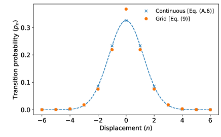
Figure 5: Comparison of $p_{n}$ [Eq. (9) or (17)] versus Gaussian function [Eq. (20)] with $\tau=0.015$ and $\delta=0.1$.

Figure 5 plots the transition probability $p_{n}$ [Eq. (9) or (17)] and its $\delta=0$ limit (a Gaussian function) [Eq. (20)] as a function of $n$. The transition probability on a grid differs visibly from the Gaussian function in the $\delta=0$ limit especially for small $n$. Specifically, dividing the space into bins slightly increases the probability of staying in the same bin at expense of decreasing the probability to hop to the nearest or second nearest neighbors. For a greater displacement, the two plots converge because $\delta$ becomes small relative to the displacement, making the saddle point approximation asymptotically exact. At every $n$, $p_{n}$ is found nonnegative.

Equation (9) can, in principle, be generalized for any symmetric finite-difference formula. However, for such a higher-order formula, $p_{n}$ is usually no longer positive for all $n$ unless $\delta^{2}\ll{\tau}$ (in which case the space is effectively continuous). It is also to be observed that our approach is not immediately extensible to an importance sampling transformation as usually performed in the context of DMC P. J. Reynolds et al. (1982) because it breaks the Hermitian and translational symmetry of the kinetic-energy operator by introducing a drift term proportional to the first derivative of the wave function.

Appendix B Proofs of Eqs. (10)–(12)

A proof of Eq. (10) is trivial.

We have

$$p_{n} = \frac{1}{2\pi}\int_{-\pi}^{\pi}\cos(kn)\exp\left\{-\frac{2\tau}{\delta^{2}}\sin^{2}\left(\frac{k}{2}\right)\right\}dk$$

$$= \frac{1}{2\pi n}\int_{-\pi n}^{\pi n}\cos(k^{\prime})\exp\left\{-\frac{2\tau}{\delta^{2}}\sin^{2}\left(\frac{k^{\prime}}{2n}\right)\right\}dk^{\prime},$$

where $k^{\prime}=kn$. It then follows for $n\to\pm\infty$

$$p_{n} \approx \frac{1}{2\pi|n|}\int_{-\infty}^{\infty}\exp(ik^{\prime})\exp\left(-\frac{\tau k^{\prime 2}}{2\delta^{2}n^{2}}\right)dk^{\prime}$$ (21)

$$= \frac{\delta}{\sqrt{2\pi\tau}}\exp\left(-\frac{n^{2}\delta^{2}}{2\tau}\right)\geq 0.$$ (22)

Equation (22) imply that $p_{n}$ and $p_{n+1}$ are nonnegative for a sufficiently large $|n|$.

In the meantime, a recursion relationship for $p_{n}$ can be derived with integration by parts. For $n\neq 0$,

$$p_{n} = \frac{1}{2\pi}\int_{-\pi}^{\pi}\cos(kn)\exp\left\{-\frac{2\tau}{\delta^{2}}\sin^{2}\left(\frac{k}{2}\right)\right\}dk$$ (23)

$$= \frac{1}{2\pi}\left[\frac{\sin(kn)}{n}\exp\left\{-\frac{2\tau}{\delta^{2}}\sin^{2}\left(\frac{k}{2}\right)\right\}\right]^{\pi}_{-\pi}$$

$$+\frac{1}{2\pi}\int_{-\pi}^{\pi}\frac{\sin(kn)}{n}\frac{\tau\sin(k)}{\delta^{2}}\exp\left\{-\frac{2\tau}{\delta^{2}}\sin^{2}\left(\frac{k}{2}\right)\right\}dk$$

$$= \frac{\tau}{2\pi n\delta^{2}}\int_{-\pi}^{\pi}\sin(kn)\sin(k)\exp\left\{-\frac{2\tau}{\delta^{2}}\sin^{2}\left(\frac{k}{2}\right)\right\}dk$$

$$= \frac{\tau}{n\delta^{2}}\frac{p_{n-1}-p_{n+1}}{2},$$

which can be rearranged to yield

$$p_{n-1}=\frac{2n\delta^{2}}{\tau}p_{n}+p_{n+1}.$$ (24)

This proves Eq. (11) for all $n$ by mathematical induction: Starting from a sufficiently large $n$ that renders both $p_{n}$ and $p_{n+1}$ nonnegative, $n$ is decremented down to zero (vice versa for negative $n$). The foregoing also implies that $p_{n}$ is monotonically decreasing with $n\geq 0$.

Equation (12) can be proven with the Fourier transform of Dirac’s $\delta$ function,

$$\sum_{n=-\infty}^{\infty}p_{n} = \int_{-\pi}^{\pi}\left\{\frac{1}{2\pi}\sum_{n=-\infty}^{\infty}\cos(kn)\right\}\exp\left\{-\frac{2\tau}{\delta^{2}}\sin^{2}\left(\frac{k}{2}\right)\right\}dk$$ (25)

$$= \int_{-\pi}^{\pi}\delta(k)\exp\left\{-\frac{2\tau}{\delta^{2}}\sin^{2}\left(\frac{k}{2}\right)\right\}dk=1.$$

References

- Kalos (1962) M. H. Kalos, Phys. Rev. 128, 1791 (1962).
- Anderson (1975) J. B. Anderson, J. Chem. Phys. 63, 1499 (1975).
- Lüchow (2011) A. Lüchow, WIREs Comput. Mol. Sci. 1, 388 (2011).
- Klein and Pickett (1976) D. J. Klein and H. M. Pickett, J. Chem. Phys. 64, 4811 (1976).
- P. J. Reynolds et al. (1982) P. J. Reynolds, D. M. Ceperley, B. J. Alder, and W. A. Lester, Jr., J. Chem. Phys. 77, 5593 (1982).
- Troyer and Wiese (2005) M. Troyer and U.-J. Wiese, Phys. Rev. Lett. 94, 170201 (2005).
- Carlson and Kalos (1985) J. Carlson and M. H. Kalos, Phys. Rev. C 32, 1735 (1985).
- Coker and Watts (1986) D. F. Coker and R. O. Watts, Mol. Phys. 58, 1113 (1986).
- J. B. Anderson et al. (1991) J. B. Anderson, C. A. Traynor, and B. M. Boghosian, J. Chem. Phys. 95, 7418 (1991).
- Kalos (1996) M. H. Kalos, Phys. Rev. E 53, 5420 (1996).
- Kalos and Schmidt (1997) M. H. Kalos and K. E. Schmidt, J. Stat. Phys. 89, 425 (1997).
- Kalos and Pederiva (2000) M. H. Kalos and F. Pederiva, Phys. Rev. Lett. 85, 3547 (2000).
- Mishchenko (2006) Y. Mishchenko, Phys. Rev. E 73, 026706 (2006).
- M. Casula et al. (2005) M. Casula, C. Filippi, and S. Sorella, Phys. Rev. Lett. 95, 100201 (2005).
- Casula et al. (2010) M. Casula, S. Moroni, S. Sorella, and C. Filippi, J. Chem. Phys. 132, 154113 (2010).
- Spencer et al. (2012) J. S. Spencer, N. S. Blunt, and W. M. C. Foulkes, J. Chem. Phys. 136, 054110 (2012).
- Sinanoǧlu (1962) O. Sinanoǧlu, J. Chem. Phys. 36, 3198 (1962).
- Bischoff and Valeev (2013) F. A. Bischoff and E. F. Valeev, J. Chem. Phys. 139, 114106 (2013).
- Hirata et al. (2017) S. Hirata, T. Shiozaki, C. M. Johnson, and J. D. Talman, Mol. Phys. 115, 510 (2017).
- Kottmann and Bischoff (2017) J. S. Kottmann and F. A. Bischoff, J. Chem. Theory Comput. 13, 5945 (2017).
- Trotter (1959) H. F. Trotter, Proc. Amer. Math. Soc. 10, 545 (1959).
- Metropolis et al. (1953) N. Metropolis, A. W. Rosenbluth, M. N. Rosenbluth, A. H. Teller, and E. Teller, J. Chem. Phys. 21, 1087 (1953).
- C. J. Umrigar et al. (1993) C. J. Umrigar, M. P. Nightingale, and K. J. Runge, J. Chem. Phys. 99, 2865 (1993).
- An and van Leeuwen (1991) G. An and J. M. J. van Leeuwen, Phys. Rev. B 44, 9410 (1991).
- G. H. Booth et al. (2009) G. H. Booth, A. J. W. Thom, and A. Alavi, J. Chem. Phys. 131, 054106 (2009).
- Kunitsa (2019) A. A. Kunitsa, griddmc: a Python program for grid-based diffusion Monte Carlo (2019), URL https://github.com/aakunitsa/QMC_grid_theory.git.
- (27) M. Galassi, GNU Scientific Library Reference Manual (3rd ed.), URL http://www.gnu.org/software/gsl/.
- Flyvbjerg and Petersen (1989) H. Flyvbjerg and H. G. Petersen, J. Chem. Phys. 91, 461 (1989).
- Spencer (2014) J. S. Spencer, pyblock: Python module for performing blocking analysis on data containing serial correlations (2014), URL https://github.com/jsspencer/pyblock.
- D. Bressanini and P. J. Reynolds (2005) D. Bressanini and P. J. Reynolds, Phys. Rev. Lett. 95, 110201 (2005).
- Ceperley (1991) D. M. Ceperley, J. Stat. Phys. 63, 1237 (1991).
- Pekeris (1959) C. L. Pekeris, Phys. Rev. 115, 1216 (1959).
- McKoy and Winter (1968) V. McKoy and N. W. Winter, J. Chem. Phys. 48, 5514 (1968).
- Mathews and Walker (1970) J. Mathews and R. L. Walker, Mathematical Methods of Physics (W. A. Benjamin, New York, 1970), 2nd ed.