Joint detection and matching of feature points in multimodal images

Abstract

In this work, we propose a novel Convolutional Neural Network (CNN) architecture for the joint detection and matching of feature points in images acquired by different sensors using a single forward pass. The resulting feature detector is tightly coupled with the feature descriptor, in contrast to classical approaches (SIFT, etc.), where the detection phase precedes and differs from computing the descriptor. Our approach utilizes two CNN subnetworks, the first being a Siamese CNN and the second, consisting of dual non-weight-sharing CNNs. This allows simultaneous processing and fusion of the joint and disjoint cues in the multimodal image patches. The proposed approach is experimentally shown to outperform contemporary state-of-the-art schemes when applied to multiple datasets of multimodal images. It is also shown to provide repeatable feature points detections across multi-sensor images, outperforming state-of-the-art detectors. To the best of our knowledge, it is the first unified approach for the detection and matching of such images.

1 Introduction

The detection and matching of feature points in images is a fundamental task in computer vision and image processing that is applied in common computer vision tasks such as image registration [46], dense image matching, [39] and 3D reconstruction [1], to name a few. The term feature point relates to the center of an image patch, that is expected to be salient and repeatedly detected in multiple images of the same scene, which might differ by pose and appearance [26]. A detector identifies the spatial location of a feature point, and the surrounding patch is encoded by a descriptor. The detection and matching of feature points in multi-modal images, as depicted in Fig. 1, is of particular interest in remote sensing [18, 23, 19, 16] and medical imaging [36], as the fusion of such images, provides information synergy. The acquisition of the same scenes by different sensors might result in significant appearance variations, that are often nonlinear and unknown apriori, such as non-monotonic intensity mappings, contrast reversal, and non-corresponding edges and textures.

The registration of the multimodal input images $\mathbf{I}_{\mathbf{1}}$ and $\mathbf{I}_{\mathbf{2}}$ can be formulated as the estimation of a parametric (rigid, affine, etc.) global transformation $T$, by minimizing an appearance invariant similarity measures $\phi(\mathbf{I}_{\mathbf{1}},\mathbf{I}_{\mathbf{2}})$

$$T^{\ast}=\arg\min_{T}\phi(\mathbf{I}_{\mathbf{1}},T(\mathbf{I}_{\mathbf{2}})).$$ (1)

$T(\mathbf{I}_{\mathbf{2}})$ is the image $\mathbf{I}_{\mathbf{2}}$ warped towards $\mathbf{I}_{\mathbf{1}}$, according to $T$. Gradient-based approaches were applied by Irani et al. [18], and Keller et al. [19] to appearance-invariant image representations to solve Eq. 1 iteratively.

Other multimodal registration schemes are based on matching local image features such as patches, contours [23], and corners. Such approaches match the sets of interest points $S_{1}\in\mathbf{I}_{\mathbf{1}}$ and $S_{2}\in\mathbf{I}_{\mathbf{2}}$, where each feature point is first detected and then encoded by a robust appearance-invariant descriptor. A pair of descriptors can be matched by computing their $L_{2}$ distance.

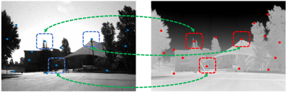
Figure 1: The multisensor patch matching problem. The matched optical (left) and IR (right) images differ by significant appearance changes due to the dissimilar physical characteristics captured by the different sensors. The images are part of the LWIR-RGB dataset [3]. The feature points in both images were detected using the proposed scheme.

Such descriptors were commonly derived by extending unimodal descriptors such as SIFT [26] and Daisy [38] to the multimodal case [10, 17, 3, 2, 21].

Convolutional Neural Networks (CNNs) were applied to feature point matching [4], by training data-driven multimodal image descriptors. These CNNs are trained by optimizing a Hinge Loss applied to an $L_{1}$ or $L_{2}$ metrics, while others [45, 5, 13, 31] aim to compute a similarity score between image patches by optimizing the Cross-Entropy loss by classifying the pairs of patches as same/not-same. Such approaches utilize Siamese CNNs [4] consisting of weight sharing sub-networks.

The upside of $L_{2}$-based representations compared to those computed using the Cross-Entropy loss is their reduced computational complexity when applied to match sets of feature points detected in a pair or set of images. As an image typically contains $n=300-500$ feature points, matching a pair of images requires $n^{2}/2$ point-to-point similarity evaluations. $K$ nearest neighbors (KNN) similarity search via $L_{2}$-based representations can be computationally accelerated using metric embedding schemes such as Locality Sensitive Hashing (LSH) [14] and MinHash [8].

Feature detectors are commonly applied to each image separately, without relating the detections in one modality to the other. A detector aims to detect the spatial location of the feature point and estimate its local scale and orientation. The location is often determined using a corner detector [26], and the local scale is computed using the Difference of Gaussians (DoG) operator and its approximations [25, 26].

In this work, we propose a CNN-based metric learning approach for the joint detection and matching of feature points in multimodal images, using a single forward pass. When applied to image patches, the proposed scheme computes the corresponding descriptors and similarity. But, when applied to full-scale images, the proposed fully convolutional CNN computes a grid of descriptors. By propagating back through the corresponding CNN activations and layers, the locations of feature points corresponding to each descriptor are detected. As the CNN is trained to optimize the descriptors’ matching, the proposed detector is tightly coupled with the feature descriptor, in contrast to classical approaches such as SIFT [26] and its (many) extensions, where the detector is computed separately before computing the descriptor. To the best of our knowledge, we introduce the first unified approach for the detection and matching of multi-modality images.

In particular, we present the Hybrid CNN architecture consisting of both a Siamese sub-network and a dual-channel non-weight-sharing asymmetric sub-network. The use of the asymmetric sub-network is due to the inherent asymmetry in the multisensor matching problem, where the heterogeneous inputs might differ significantly, and thus require different processing implemented by the asymmetric sub-network. In particular, each branch of the asymmetric sub-network estimates a modality-specific adaptive representation of the multisensor patches.

Thus, we aim to leverage both the joint and disjoint attributes in the multimodal images, using the Siamese and Asymmetric subnets, respectively. Siamese sub-networks were previously shown [4] to yield accurate matching results, and are outperformed by the proposed Hybrid scheme. The Siamese and Asymmetric subnets are trained by corresponding losses, and their outputs are merged and optimized to yield a fused image representation.

In particular, we propose the following contributions:

First, we present a novel approach for the joint detection and matching of feature points in multi-modality images.

Second, the proposed scheme is implemented using a novel Hybrid CNN architecture consisting of both a Siamese and asymmetric sub-networks, able to leverage both the joint and disjoint cues in multimodal patches, to determine their similarity.

Third, we show that training the proposed Hybrid CNN by multi-loss learning improves the descriptors’ matching accuracy.

Last, the proposed scheme was experimentally shown to outperform contemporary approaches when applied to state-of-the-art multimodal image matching benchmarks [4, 5, 13] and feature points detection schemes. The corresponding source code was made publicly available.

2 Related work

2.1 Appearance-invariant image representations

The matching of multi sensor images has been studied in a gamut of works. Earlier, unsupervised approaches were mostly based  on deriving appearance-invariant image representations of multisensor images, that utilized salient image edges and contours. Thus, Irani et al. [18] suggested a coarse-to-fine scheme for estimating the global parametric motion (affine, rigid) between multimodal images, using the magnitudes of directional derivatives as a robust image representation. The correlation between these representations is maximized using iterative gradient methods and a coarse-to-fine formulation.

The “Implicit Similarity” formulation by Keller et al. [19] is an iterative scheme utilizing gradient information for global alignment. A set of pixels with maximal gradient magnitude is detected in one of the input images, rather than contours and edges as in [18]. The gradient of the corresponding points in the second image is maximized with respect to a global parametric motion, without explicitly maximizing a similarity measure. The seminal work of Viola and Wells [40] proposed an appearance-robust image representation based on the statistical representations of the images. The mutual information between these representations was optimized with respect to the motion parameters.

Modality-invariant local descriptors were derived by modifying the SIFT descriptor [10, 27]. Contrast-invariance was achieved by mapping the gradient orientations of the interest points from $[0,2\pi)$ to $[0,\pi)$. Hasan et al. showed that such descriptors mitigate the matching accuracy [17], and further modified the SIFT descriptor [16] by thresholding gradient values to reduce the effect of strong edges. An enlarged spatial window with additional sub-windows was used to improve the spatial resolution. Aguilera et al. [3] used a histogram of contours and edges instead of a histogram of gradients to avoid the ambiguity of the SIFT descriptor when applied to multimodal images, while the dominant orientation was determined similarly. This approach was extended by the same authors by using multi-oriented and multi-scale Log-Gabor filters [2].

2.2 Structural similarity

Geometrical structure was used as an appearance-invariant representation, where the similarity was quantified by structural similarity. Hence, the Self Similarity Matching (SSM) approach by Shechtman et al. [34] is a geometric descriptor encoding the local geometric structure around a feature point in an image, by correlating a central patch to all adjacent patches within a predefined radius. The Dense Adaptive Self-Correlation (DASC) descriptor, by Kim et al. [20], extended the SSM approach, by computing the self-similarity measure as an adaptive self-correlation between randomly sampled patches.

2.3 Deep learning approaches

With the emergence of CNNs as the state-of-the-art approach to a gamut of computer vision problems, CNNs were applied to patch matching. Siamese CNNs such as HardNet  [29], L2-Net  [37] and MatchNet [43] were applied to matching single modality images, significantly outperforming the classical handcrafted image features.

Zagoruyko and Komodakis [45] proposed several CNN architectures for multisensor feature matching, using a Siamese CNN with a Contrastive or Cross-Entropy losses, for matching single modality patches, and a CNN, where the input patches are stacked as different image channels. Aguilera et al. [4] applied the approaches by Zagoruyko and Komodakis [45] to matching multimodal patches and showed that the resulting CNN outperformed the state-of-the-art multimodal descriptors.

To alleviate the computational complexity of the stacked approach when applied to sets of feature points, Aguilera et al. proposed the Q-Net CNN [5] that was trained using an $L_{2}$ loss. The Q-Net CNN consists of four weight sharing sub-networks and two corresponding pairs of input patches, that allow hard negative mining [29]. This approach was shown to achieve state-of-the-art accuracy when applied to the Vis-Nir benchmark [4].

En et al. [13] introduced a simplified Hybrid-like CNN, denoted as TS-Net, for multimodal patch matching, utilizing a Cross-Entropy loss. Contrary to the proposed scheme, this approach does not compute $L_{2}$-optimized patch encodings, that are essential for matching images, typically consisting of 300-500 feature points. Each of the sub-networks outputs a scalar Softmax prediction that are merged using a FC layer. In contrast, we utilize a different architecture where feature maps are fused, and apply auxiliary losses (that are not used by En et al. [13]).

Metric learning was applied by Quan et al. [30] to learn the shared feature space of multi-spectral patches, by progressively comparing spatially connected features, using a discrimination constraint (SCFDM). This approach was extended by the same authors, by deriving the AFD-Net [31], that learns multiscale joint multi-spectral features using a CNN consisting of two subnetworks. The activations maps at different layers are subtracted, and the differences are propagated through multiple FC layers. Thus, this approach does not compute a descriptor, and the matching of two images having $n$ feature points each, entails $n^{2}/2$ forward passes of the CNN, in contrast, to the single forward pass required by the proposed scheme. A novel metric learning cost function denoted the Exponential Loss, was introduced by Wang et al. for patch matching [41]. Using a corresponding hard negative mining scheme, it was shown to provide SOTA accuracy on the VIS-NIR dataset [4].

The joint detection and matching of feature points in single modality images was first suggested by Yi et al. [44] that proposed the LIFT scheme using a Siamese CNN. LIFT consists of three successive parts: a feature point detector, followed by an estimate of the detected point’s orientation (similar to the dominant orientation in SIFT), and the feature point descriptor. Dusmanu et al. [12] also proposed a Siamese network, where the descriptors are trained using a triplet ranking loss, and the features are detected as the local maxima of the last activation map. The corresponding CNN was implemented without pooling layers to relate the detections in the last activation map to the source (finest) image resolution. The model was trained using pixel correspondences computed by large-scale SfM reconstructions. An image pyramid consisting of three resolutions is used to account for scale variations, by computing the descriptors in all scales.

Simeoni et al. [35] proposed a multi-scale feature detection scheme for single modality images by detecting local maxima in the activation maps over multiple activation layers. The activations are localized per channel using the maximally stable extremal regions (MSER) blob detector. As in [12], a Siamese network is used to match the corresponding detections in the training images.

3 Detection and matching of multi-modal feature points

Let $\mathbf{x}_{i}\in\mathbf{I}_{\mathbf{1}}$ and $\mathbf{y}_{i}\in\mathbf{I}_{\mathbf{2}}$ be a pair of multi-dimensional image patches acquired by different modalities. We aim to compute a corresponding representation, $\widehat{\mathbf{x}_{i}}$ and $\widehat{\mathbf{y}_{i}}$, respectively. The Hybrid network learns both the joint and disjoint characteristics of the multisensor patches, using both Siamese (symmetric) and asymmetric (non-weight-sharing) networks. The Siamese network learns the same mapping for both input modalities, denoted as ${W}_{{s}}(\mathbf{x}_{i})$ and ${W}_{{s}}(\mathbf{y}_{i})$ in Fig. 2, respectively, allowing to encode the same characteristics between the images. The asymmetric network estimates different, modality-specific representations, ${W}_{x}(\mathbf{x}_{i})$ and ${W}_{y}(\mathbf{y}_{i})$, for each modality, respectively. The outputs of the symmetric and asymmetric sub-networks are concatenated

$$H_{x}(\mathbf{x}_{i}) =\left[{W}_{{s}}(\mathbf{x}_{i}),{W}_{x}(\mathbf{x}_{i})\right]^{T},$$ (2)

$$H_{y}(\mathbf{y}_{i}) =\left[{W}_{{s}}(\mathbf{y}_{i}),{W}_{y}(\mathbf{y}_{i})\right]^{T},$$

and the resulting Hybrid representation is given by

$$\widehat{\mathbf{x}_{i}} =FC_{x}(H_{x}(\mathbf{x}_{i})),$$ (3)

$$\widehat{\mathbf{y}_{i}} =FC_{y}(H_{y}(\mathbf{y}_{i}))$$

where $FC_{x}$ and $FC_{y}$ are FC layers.

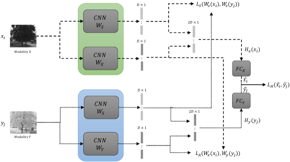
Figure 2: The proposed hybrid matching model. The model consists of two sub-networks: a siamese subnetwork and an asymmetric subnetwork with non-shared weights. The siamese branch consists of a pair of $W_{s}$ CNNs and is trained by the loss $L_{s}$. The asymmetric branch consists of the $W_{x}$ and $W_{y}$ CNNs and is trained by the loss $L_{A}$. The symmetric and asymmetric representations are merged and trained by the loss $L_{H}$.

The proposed CNN is fully convolutional and can thus be applied to images of varying dimensions. When applied to $64\times 64$ image patches, the Hybrid CNN yields a pair of $\{\widehat{\mathbf{x}_{i}},\widehat{\mathbf{y}_{i}}\}\in\mathbb{R}^{128}$ descriptors. But, when applied to larger images, an activation map $\{\widehat{\mathbf{x}_{i,j}},\widehat{\mathbf{y}_{i,j}}\}\in\mathbb{R}^{128}$ is computed. Each descriptor relates to a particular patch in the image, according to its footprint. We show that by backtracking through the CNN activations, down to the input layer, we detect the location of the corresponding feature points in the finest image resolution, as detailed in Section 3.2.

The proposed CNN is trained using multiple losses. The losses $L_{S}$ and $L_{A}\,$in Fig. 2 optimize the symmetric and asymmetric subnetworks, respectively. This was shown to improve the matching accuracy, as these losses ($L_{S}$ and $L_{A}$) optimize CNNs having less number of parameters compared to the full Hybrid CNN. The unified Hybrid representation, as in Eq. 3, is trained using the $L_{H}$ loss.

We used both the Binary Cross-Entropy (BCE) and the Contrastive Loss (CL) [15]. The CL is give by

$$L_{C}\left(x_{i},x_{j},x_{k}\right)=\frac{1}{\left|Pos\right|}{\displaystyle\sum\limits_{x_{i},x_{j}\in Pos}}D^{2}\left(x_{i},x_{j}\right)+\\ \frac{1}{\left|Neg\right|}{\displaystyle\sum\limits_{x_{i}\in Pos,x_{k}\in Neg}}\left[m-D^{2}\left(x_{i},x_{k}\right)\right]_{+}$$ (4)

where $\left[\cdot\right]_{+}$ is the Hinge loss operator, and $D\left(x_{i},x_{j}\right)$ is the $L_{2}$ distance between the embeddings. $m$ is a predefined threshold that is commonly defined as $m=1$ for $L_{2}$ normalized embeddings, as in our CNN.

All losses $\{L_{S},L_{A},L_{H}\}$ are either all BCE or CL. The choice of the loss relates to the particular task of the multi-modality descriptors $\widehat{\mathbf{x}_{i}}$ and $\widehat{\mathbf{y}_{i}}$. For the BCE-based descriptors, a Softmax layer outputs the matching probability of the input patches, while the CL yields a descriptor embedded in a Euclidean space. Such descriptors can be utilized in efficient large-scale descriptor retrieval schemes, where $K$-nearest-neighbors (KNN) $L_{2}$ search can be efficiently implemented using LSH [14] and MinHash [8].

3.1 CNN architecture

The proposed networks consist of a Siamese (symmetric) and asymmetric networks, as depicted in Fig. 2. The Siamese network consists of the two weight-sharing networks $W_{s}$, while the asymmetric network consists of the non-weight-sharing networks $\{W_{X},W_{Y}\}$ applied to the inputs $X$ and $Y$, respectively. When the losses $\{L_{S},L_{A},L_{H}\}$ are all Contrastive losses, $W_{X},W_{Y}$ and $W_{s}$ are detailed in Table I.

Layer	Output	Kernel	Stride	Pad
Conv0	$64\times 64\times 32$	$5\times 5$	1	2
Pooling	$32\times 32\times 32$	$3\times 3$	2	-
Conv1	$32\times 32\times 64$	$5\times 5$	1	2
Pooling	$16\times 16\times 64$	$3\times 3$	2	-
Conv2	$16\times 16\times 128$	$3\times 3$	1	1
Pooling	$8\times 8\times 128$	$3\times 3$	2	-
Conv3	$6\times 6\times 256$	$3\times 3$	1	0
Conv4	$4\times 4\times 256$	$3\times 3$	1	0
FC	$1\times 1\times 128$	-	-	-
Unit norm	$1\times 1\times 128$	-	-	-

TABLE I: The CNN architecture of the sub-networks using the Contrastive Loss. Each sub-network accepts a $64\times 64$ patch and outputs a $128\times 1$ descriptor. ReLU activations are applied after each pooling layer, as well as after the Conv3 layer.

Similarly, when the losses $\{L_{S},L_{A},L_{H}\}$ are all BCE losses, $W_{X},W_{Y}$ and $W_{s}$ are given by Table II, and the overall training loss is given by

$$L=L_{S}+L_{A}+L_{H}$$ (5)

Layer	Output	Kernel	Stride	Pad
Conv0	$64\times 64\times 32$	$5\times 5$	1	2
Pooling	$32\times 32\times 32$	$3\times 3$	2	-
Conv1	$32\times 32\times 64$	$5\times 5$	1	2
Pooling	$16\times 16\times 64$	$3\times 3$	2	-
Conv2	$16\times 16\times 128$	$3\times 3$	1	1
Pooling	$8\times 8\times 128$	$3\times 3$	2	-
Conv3	$6\times 6\times 256$	$3\times 3$	1	0
Conv4	$4\times 4\times 256$	$3\times 3$	1	0
Conv5	$2\times 2\times 256$	$3\times 3$	1	0
FC	$1\times 1\times 128$	-	-	-

TABLE II: The CNN architecture of the sub-networks using the Cross-Entropy loss. Each sub-network accepts a $64\times 64$ patch and outputs a $128\times 1$ descriptor. ReLU activations are applied after each pooling layer, as well as after the Conv3 and Conv4 layers.

3.2 The detection of feature points in multi-modality images

A feature point $\mathbf{v}=\left(l,k\right)$ is a pixel location, such that the feature points $\mathbf{v}_{x}\in\mathbf{I}_{\mathbf{1}}$ and $\mathbf{v}_{y}\in\mathbf{I}_{\mathbf{2}}$ relate to the descriptors $\widehat{\mathbf{x}}$ and $\widehat{\mathbf{y}}$, respectively. The fundamental property of a feature point is its repeatability [26, 28], implying that corresponding points $\mathbf{v}_{x}\in\mathbf{I}_{\mathbf{1}}$ and $\mathbf{v}_{y}\in\mathbf{I}_{\mathbf{2}}$ relate to joint image content in both images.

We propose to detect the feature points by analyzing the joint representation encoded by the Siamese subnetworks $\widehat{\mathbf{x}_{i}^{s}}={W}_{{s}}(\mathbf{x}_{i})$ and $\widehat{\mathbf{y}_{i}^{s}}={W}_{{s}}(\mathbf{y}_{i})$ (as in Fig. 2) to detect $\mathbf{v}_{x}\in\mathbf{I}_{\mathbf{1}}$, and $\mathbf{v}_{y}\in\mathbf{I}_{\mathbf{2}}$, respectively. We also applied the asymmetric subnetworks ${W}_{{x}}(\mathbf{x}_{i})$ and ${W}_{{y}}(\mathbf{y}_{i}),$ resulting in less accurate results.

The proposed Hybrid patch-matching scheme is implemented by fully convolutional CNNs. Thus, when ${W}_{{s}}(\mathbf{x}_{i})$ and ${W}_{{s}}(\mathbf{y}_{i})$ are applied to $64\times 64$ patches, the result is $\in\mathbb{R}^{128\times 1}$. But, when applied to images $\in\mathbb{R}^{W\times H\times 3},$ their outputs are activation maps $\in\mathbb{R}^{\frac{W}{64}\times\frac{H}{64}\times C}$, where $C$ is the number of channels in the activation map. Hence, each point in ${W}_{{s}}(\mathbf{x}_{i})$ and ${W}_{{s}}(\mathbf{y}_{i})$ encodes an image patch $\mathbf{P}\in\mathbb{R}^{64\times 64\times 3}$. As the Hybrid CNN is trained to optimize the matching between the $\mathbf{x}$ and $\mathbf{y}$ modalities, ${W}_{{s}}$ is also jointly optimized to extract the most informative features from the corresponding images patches $\left\{\mathbf{P}_{i,j}\right\}$. The locations of the largest activations are the more informative, and the locations with smaller values are pruned by the max-pooling layers.

Thus, the core of our approach is to detect the informative feature points in the input image given the activation map $\widehat{\mathbf{x}_{i}^{s}}={W}_{{s}}(\mathbf{x}_{i})\in\mathbb{R}^{\frac{W}{64}\times\frac{H}{64}\times C}$ .  The detection is applied by backtracking the spatial locations of the activation $\widehat{\mathbf{x}_{i}^{s}}$ through ${W}_{{s}},$ down to the first activation layer to identify the pixels contributing to ${W}_{{s}}(\mathbf{x}_{i})$. In contrast to those that were pruned by the max-pooling layers.

3.2.1 Backtracking for feature detection

The ${W}_{{s}}$ CNN, detailed in Tables I and II, consists of padded convolutions and pooling layers. Let $\widehat{\mathbf{x}}^{l}\in\mathbb{R}^{w_{l}\times h_{l}\times c_{l}}$  be the activation map at level $l$ of spatial dimensions $w_{l}\times h_{l}$ and $c_{l}$ channels. Spatially symmetric (i.e. $3\times 3$) padded convolutions do not change the locations of the activations, such that each element $\widehat{\mathbf{x}}_{i,j}^{l}\in\widehat{\mathbf{x}}^{l}$ corresponds to the same spatial location in the preceding activation map $\widehat{\mathbf{x}}_{i,j}^{l-1}\in\widehat{\mathbf{x}}^{l-1}$. This implies that when backtracking through a symmetric convolution layer, we have that $\widehat{\mathbf{x}}_{i,j}^{l}\rightarrow\widehat{\mathbf{x}}_{i,j}^{l-1}$.

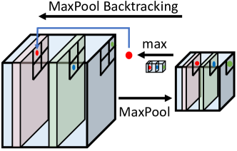
Figure 3: Backtracking a $2\times 2$ max-pooling layer. In the forward pass (left to right), multiple spatial locations are mapped by the max-pooling layer to a single spatial location. In the backtracking pass (right to left), the maximum over all channels in a particular spatial location (red dot), is the one propagated back.

In contrast, max-pooling layers propagate the content of multiple spatial locations in the activation map $\widehat{\mathbf{x}}^{l-1}$ to a single spatial location in the succeeding layer $\widehat{\mathbf{x}}^{l}$, as depicted in Fig. 3. Let $\widehat{\mathbf{x}}^{l-1}\in\mathbb{R}^{W\times H\times C}$ and $\widehat{\mathbf{x}}^{l}\in\mathbb{R}^{\frac{W}{k}\times\frac{H}{k}\times C}$ be the input and output layers, respectively, of a $k\times k$ max-pooling layer. For each $k\times k\times 1\in$ $\widehat{\mathbf{x}}^{l-1}$, the entry having the maximal value is propagated forward. Thus, the entries in a single particular spatial location $\widehat{\mathbf{x}}^{l}\left(w,h,c\right),$ $c=1..C$ might correspond to multiple spatial locations in $\widehat{\mathbf{x}}^{l-1}$. To relate these entries to a single spatial location in $\widehat{\mathbf{x}}^{l-1}$, we only backtrack the spatial location of the entry $\widehat{\mathbf{x}}^{l}\left(\frac{w}{k},\frac{h}{k},c^{\ast}\right)$ having the maximal activation

$$c^{\ast}=\arg\underset{c}{\max}\left\{\widehat{\mathbf{x}}^{l}\left(\frac{w}{k},\frac{h}{k},c\right)\right\},c=1..C,$$ (6)

corresponding to a single spatial location in $\widehat{\mathbf{x}}^{l-1}$, as in Fig. 3.

The feature points are given by the locations of the backtracked maximal activations $\mathbf{V}\in\mathbb{R}^{\frac{W}{64}\times\frac{H}{64}\times 2}$. The corresponding activations are the detections scores, similar to the DoG detections scores used in the SIFT DoG-based detector [26]. It is common to only utilize a subset of the ‘best’ detected points, by choosing the $N$ feature points having the largest detection score, or the points having a detection score larger than a predefined threshold.

The proposed detection approach differs from Dusmanu et al. [12] that compute local (per layer) detection scores, and merge the scores from different layers, having different spatial resolutions, by bilinearly interpolating the lower-resolution score maps. Simeoni et al. [35] utilize a CNN without pooling layers to avoid backtracking through the activation layers. Both these schemes are only applicable to single-modality images.

4 Experimental Results

The proposed Hybrid scheme was experimentally verified by applying it to multi-spectral image datasets and benchmarks used in contemporary state-of-the-art matching schemes. The first was suggested by Aguilera et al. [4] consisting of a set of matching and non-matching pairs of patches, extracted from nine categories of the public VIS-NIR scene dataset [9]. The feature points were detected by an interest point detector and matched manually. We also used the Vehicle Detection in Aerial Imagery (VEDAI) [32] dataset of multispectral aerial images and the CUHK [42] dataset consisting of 188 faces and corresponding sketches drawn by artists. These multimodal datasets are spatially pre-aligned, same as the VIS-NIR dataset, and were used by En et al. [13] to create annotated training and test sets by extracting corresponding pairs of patches on a uniform grid. We denote the uniformly-extracted VIS-NIR dataset by En et al. as Uniform VIS-NIR (UVIS-NIR) to differentiate it from the one by Aguilera et al. [4].

We evaluated the matching of the proposed scheme following the experimental setups and datasets used by Aguilera et al. [4, 5] and En et al. [13] and the results are detailed in Sections 4.2 and 4.3, respectively. The matching quality is quantified by the false positive rate at 95% recall (FPR95), same as in [4, 5]. FPR95 evaluate how well our approach distinguishes correct and incorrect matches. The source code of the proposed scheme was made publicly available.

We compare the results of the proposed Hybrid scheme using both Contrastive and Cross-Entropy losses to contemporary state-of-the-art approaches in Sections 4.2 and 4.3. The detection accuracy and an ablation study are discussed in Sections 4.4 and 4.5.

4.1 Training

The Hybrid CNN was trained using stochastic gradient descent with a momentum of 0.9, batch size of 128, learning rate of $0.01$ and weight decay of 0.0005, where the same hyperparameters were used for training both the Contrastive and Cross-Entropy losses. The Hybrid model was trained for 40 and 100 epochs, for the Contrastive and Cross-Entropy losses, respectively. In both setups, patches of 64x64 pixels were cropped and augmented by joint random rotations of $90{{}^{\circ}}$, as well as horizontal and vertical flipping. The patches of each imaging modality were normalized separately by subtracting their mean. In each training set, as in Sections 4.2 and 4.3, the positive pairs of patches are given, and any other pairing can be considered negative.

We start the training using random negative pairs, the same number as the positive ones. A training batch consists of pairs of randomly chosen corresponding (positive) pairs of patches, and negative pairs are chosen by randomly ordering the patches related to both sensors. After the loss is not reduced for $m=3$ epochs, we switch to hard negative mining for the remainder of the training. The hard mining is an adaptation of the Hardnet approach of Mishchuk et al. [29]. In each batch, the negative pairs of patches are chosen by first, computing the distances between all pairs of patches related to different modalities. Each patch is then paired with the most similar unrelated patch from the other modality, to form the hard negative pairs. The networks’ parameters were initialized by a normal distribution, where the asymmetric subnets were initialized identically to improve convergence.

Network/descriptor	Field	Forest	Indoor	Mountain	Old building	Street	Urban	Water	Mean
Engineered Features
SIFT [26]	39.44	11.39	10.13	28.63	19.69	31.14	10.95	40.33	23.95
Inv SIFT [27]	34.01	22.75	12.77	22.05	15.99	25.24	17.44	32.33	24.42
LGHD [2]	16.52	3.78	7.91	10.66	7.91	6.55	7.21	12.76	9.16
LSS [34]	46	42.48	37.14	42.5	42.35	44.5	34.9	46	42.65
DASC [20]	46.68	35.38	23.19	41.29	38.07	39.02	12.28	45.6	36.68
Learning-based
Siamese [4]	15.79	10.76	11.6	11.15	5.27	7.51	4.6	10.21	9.61
Pseudo Siamese [4]	17.01	9.82	11.17	11.86	6.75	8.25	5.65	12.04	10.32
2Channe l[4]	9.96	0.12	4.4	8.89	2.3	2.18	1.58	6.4	4.47
Q-Net 2P-4N [5]	17.01	2.70	6.16	9.61	4.61	3.99	2.83	8.44	6.86
SCFDM [30]	7.91	0.87	3.93	5.07	2.27	2.22	0.95	4.75	3.48
L2-Net [37]	16.77	0.76	2.07	5.98	1.89	2.83	0.62	11.11	5.25
HardNet [29]	10.89	0.22	1.87	3.09	1.32	1.30	1.19	2.54	2.80
Exp-TLoss [41]	5.55	0.24	2.30	1.51	1.45	2.15	1.44	1.95	2.07
Hybrid CNN
Hybrid-CL	4.61	0.22	2.52	2.69	1.52	1.34	1.55	2.22	1.93
D-Hybrid-CL	4.4	0.20	2.48	1.50	1.19	1.93	0.78	1.56	1.7

TABLE III: Patch matching results evaluated using the VIS-NIR dataset. The patches were extracted as in Aguilera et al. [4, 5]. The accuracy is given in terms of the FPR95 score. Hybrid-CL is the implantation of the proposed scheme using the CNN, as in Section 3.1, while D-Hybrid-CL utilizes the deeper CNN, as in Wang et al. [41].

4.2 VIS-NIR benchmark

The proposed Hybrid scheme was experimentally evaluated using the VIS-NIR dataset [4], and was compared to the previous results, all using the same experimental setup as in Aguilera et al. [4, 5] and En et al. [13]. All of the schemes were trained using the ’Country’ category, where we utilized $80\%$ of the given training pairs of patches for training, and the remaining $20\%$ for evaluation. The results are reported in Table III. We compared against several classes of previous works. First, we studied the accuracy of handcrafted local descriptors such as LSS [34], DASC [20], LGHD [2], SIFT [26] and MI-SIFT [27] using their publicly available code. Such schemes are shown to be notably outperformed by recent learning-based approaches, including ours. The LSS and DASC performed worse, as such descriptors aim to encode corresponding large-scale geometrical patterns that might not exist in multisensor images. Second, we compared to HardNet [29] and L2-Net  [37] that are recent, general-purpose patch matching schemes, based an a siamese CNN, which were specifically trained using the VIS-NIR dataset protocol by Wang et al.  [41]. Last, we compared to recent the SOTA multi modal results of SCFDM [30] and Wang et al.  [41], that also utilized the same dataset and experimental se up.

Our scheme outperforms HardNet  [29] and L2-Net  [37] by 64% and 200%, respectively. Wang et al.  [41] presented the recent SOTA results, using a deeper CNN than the one detailed in Section 3.1. Hence, we report the results of two implementations of the proposed Hybrid scheme. The first Hybrid-CL (Contrastive Loss), utilizes the CNN detailed in Table I as a base CNN for the symmetric and asymmetric branches, and is further used in the following sections. The second, denoted D-Hybrid-CL was implemented using the deeper CNN of Wang et al.  [41]. Both of our schemes outperform the previous SOTA (Wang et al.  [41])  by 17%, where the deeper CNN is shown to provide additional accuracy.

4.3 En et al. [13] benchmark

We also evaluated the proposed scheme using the experimental setup proposed by En et al. [13] where the VEDAI [32], CUHK [42] and VIS-NIR [4] datasets were sampled on a uniform grid, and the results are reported in Table IV. We quote the results reported by En et al. [13] for these datasets and setup, and trained the publicly available code of Aguilera et al. [4, 5] and the proposed Hybrid scheme, using $70\%$ of the data in each dataset for training, $10\%$ for validation and $20\%$ for testing. As before we compared with the results of the SIFT [26] and modality-invariant descriptors: LSS [34], DASC [20], LGHD [2] and MI-SIFT [27].

It follows that the proposed approach significantly outperformed the previous schemes for the UVIS-NIR and CUHK datasets yielding an average error that is threefold more accurate. For the VEDAI dataset, both Aguilera et al. [4], and the proposed scheme achieved a zero error. To further validate these results, we trained the VEDAI matching network 10 times, each time starting from a different random initialization of the CNN weights. We achieved zero error in all of the trained CNNs and a corresponding standard deviation (STD) of $\sigma=0$. We also computed the FPR99 and also achieved zero error and STD of $\sigma=0$. This superior performance is achieved without applying hard-mining, emphasizing that the Hybrid CNN formulation is the one doing the heavy lifting. In particular, comparing to the TS-Net [13], our approach is 3-20 times more accurate.

Network/descriptor	VEDAI	CUHK	UVIS-NIR
Engineered Features
SIFT[26]	42.74	5.87	32.53
Inv SIFT [27]	11.33	7.34	27.71
LSS[34]	39.9	43.11	42.25
DASC[20]	8.9	43.05	38.1
LGHD[2]	1.31	0.65	10.76
Learning-based
2Channel[4]	0	0.39	11.32
Q-Net 2P-4N[5]	0.78	0.9	22.5
Siamese[13]	0.84	3.38	13.17
Pseudo Siamese[13]	1.37	3.7	15.6
TS-Net[13]	0.45	2.77	11.86
Hybrid CNN
Hybrid-CE	0	0.05	3.66
Hybrid-CL	0,$\sigma=0$	0.1	3.41
Hybrid-CL FPR99	0,$\sigma=0$	-	-

TABLE IV: Patch matching results evaluated using the UVIS-NIR, VEDAI and CUHK datasets. The patches were extracted using a uniform lattice layout as in En et al. [13]. The accuracy is given in terms of the FPR95 score. The schemes names in bold are variations of the proposed scheme, CE and CL relates to using the Cross-Entropy and Contrastive losses, respectively. For the VEDAI dataset, we trained the Hybrid-CL ten times, starting from random weights and also report the standard deviation $\sigma$, and the FPR99 results.

4.4 Features detection

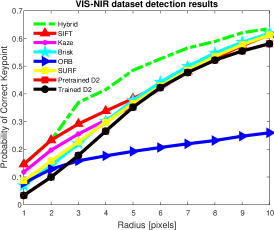
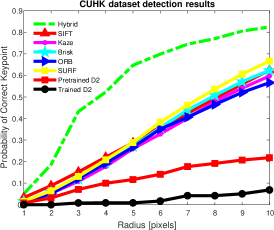
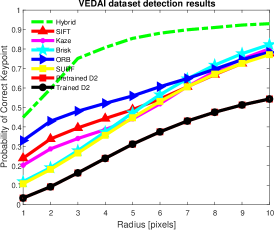
Figure 4: Feature detection results. We report the Probability of Correct Keypoint [11] and compare with handcrafted detectors and the D2-Net [12]. (a) VIS-NIR dataset results. The images and detection maps are 680$\times$1024 and 78$\times$121, respectively. (b) CUHK dataset results. The images and detection maps are 250$\times$200 and 24$\times$18, respectively. (c) VEDAI dataset results. The images and detection maps are 512$\times$512 and 57$\times$57, respectively.

The proposed feature point detection scheme, introduced in Section 3.2, was experimentally evaluated following Mikolajczyk and Schmid [28]. The detection repeatability was measured using the VEDAI [32], CUHK [42] and VIS-NIR [4] image sets consisting of aligned multimodal images. Thus, for each point $\mathbf{v}_{1}^{i}\in\mathbf{I}_{\mathbf{1}}$, there is a groundtruth corresponding point $\mathbf{v}_{2}^{i}\in\mathbf{I}_{\mathbf{2}}$. Let $\mathbf{v}_{1}^{d}\in\mathbf{I}_{\mathbf{1}}$ be a detected feature point, whose corresponding groundtruth point is $\mathbf{v}_{2}^{d}\in\mathbf{I}_{\mathbf{2}}$, and let $\mathbf{v}_{2}^{d^{\ast}}\in\mathbf{I}_{\mathbf{2}}$ be the detected point that is the closest to $\mathbf{v}_{2}^{d}$. We report the Probability of Correct Keypoints [11]

$$P_{C}=P\left(\left|\mathbf{v}_{2}^{d}-\mathbf{v}_{2}^{d^{\ast}}\right|_{2}\leq r\right),\text{ }r\in\mathbb{R}^{+},$$ (7)

that is the average probability (over all detected points $\mathbf{v}_{1}^{d}\in\mathbf{I}_{\mathbf{1}}$) that the closest feature point $\mathbf{v}_{2}^{d}\in\mathbf{I}_{\mathbf{2}}$ was detected within a radius $r$ of the groundtruth match $\mathbf{v}_{2}^{d}$. For each pair of images, we compute $P_{C}$ twice by switching $\mathbf{I}_{\mathbf{1}}$ and $\mathbf{I}_{\mathbf{2}}$ and averaging the results.

The proposed Hybrid detector provides a fixed detection grid, while detectors such as SIFT detect a varying number of feature points per image, as they utilize a cornerness score that is compared with a detection threshold. For instance, the VIS-NIR dataset consists of 680$\times$1024 images, resulting in 78$\times$121 detection maps, while the SIFT typically detects $\sim 500$ feature points at most per image. Denote $N_{s}\left(I\right)$ as the number of SIFT-based feature points detected in an image $I$. A denser detection grid might result in a higher detection probability $P_{C}$. Thus, to allow a fair comparison, we utilize $N_{s}\left(I\right)$ feature points per image for all detectors. The points in the Hybrid-based detection map are sorted by their activation, and the leading $N_{s}\left(I\right)$ feature points are retained.

We first compared the proposed detector to classical handcrafted detectors: SIFT [26], SURF [7], KAZE [6], BRISK [22], and ORB [33] detectors. Handcrafted detectors, in contrast to descriptors are not modality-specific, making the comparison valid. We also compared to the deep learning-based D2-Net [12]  detection and matching CNN. For that, we first compare to a pretrained D2-Net, that was trained on RGB images with significant appearance variations (day, night, shadows etc.). We also trained a D2-Net on the different multimodal datasets according to their experimental protocols.

The detection results are shown in Fig. 4 where we report the cumulative detection probabilities as in Eq. 7. It follows that the proposed Hybrid detector significantly outperformed the handcrafted detectors and the pretrained D2-Net. The D2-Net performed best for the VIS-NIR dataset, that consists of scenes that are most similar to the D2-Net dataset. The trained D2-Net performed worse than the pretrained D2-Net and we attribute that to the smaller training sets. The pretrained D2-Net CNN was trained using the MegaDepth dataset [24] consisting of 102,681 images, that is a multiple orders of magnitude larger than the VEDAI, CUHK and VIS-NIR datasets.

We show qualitative detection results in Figs. 5, 6 and in the Supplementary materials. We compare the detections of the proposed Hybrid scheme, SIFT and the pretrained D2-Net. For each approach and particular image modality (either VIS or NIR) we show the 200 detections having the largest detection scores, that were classified as either inliers or outliers. For each detected feature point $x$ (say in Fig. 5a) we search for a detected point in the other modality image (Fig. 5b) that is within $r=5$ pixels, same as in Eq. 7. If such a point exists, $x$ is considered an inlier (green), and an outlier (red) otherwise. To exemplify the general applicability of the proposed detection scheme, we chose an image showing a natural scene in Fig. 5 mainly consisting of textures, in contrast to the urban environment in Fig. 6, that is characterized by significant edges. The Hybrid approach detects elongated edge-like features that are known to be salient and repeatable to appearance variations. It outperforms both other schemes in terms of repeatability and the number of inliers, although the D2-Net [12] was mainly trained on the urban views in the MegaDepth dataset [24].

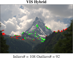
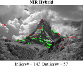
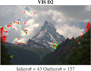
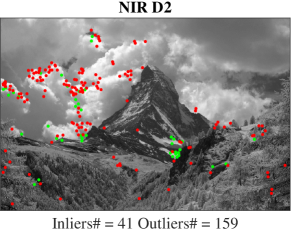
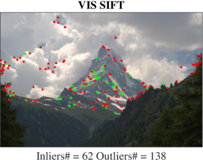
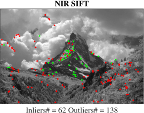
Figure 5: Qualitative feature detection results. For each approach we show the 200 detections having the largest detection scores. The inliers are marked in green, while the outliers are marked in red. Please zoom-in to view the detected points.

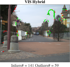
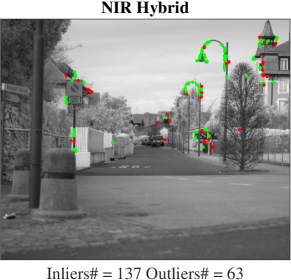
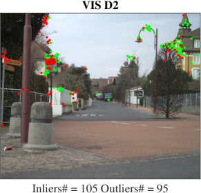
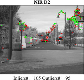
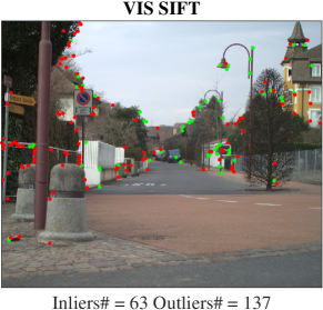
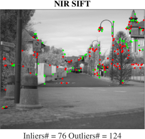
Figure 6: Qualitative feature detection results. For each approach we show the 200 detections having the largest detection scores. The inliers are marked in green, while the outliers are marked in red. Please zoom-in to view the detected points.

We also tested combined detection and matching, where the feature points were first detected and then matched by the same schemes as in Figs. 5-6 to evaluate their overall accuracy. The results are shown in Figs. 7 and 8, where we first detected 200 feature points in the IR image and matched them to 400 points detected in the corresponding RGB image, based on the $L_{2}$ distance between the descriptors. As the NIR and RGB images are pixelwise aligned, we considered the matches as inliers when the spatial distance between $L_{2}$-matched points was less than $r=5$ pixels. Otherwise the detections were considered outliers. The proposed Hybrid scheme outperformed the other schemes in all cases in terms of the number of inliers. In particular, the upside is significant for the natural scene in Fig. 7, compared to the urban scene in Fig. 8. We attribute that to D2 being trained using the urban views in the MegaDepth dataset [24], while the SIFT is handcrafted to identify corners using the DoG detector, that is more applicable to urban scenes. We also tested the complementary matchings of VIS-to-IR, and achieved similar results.

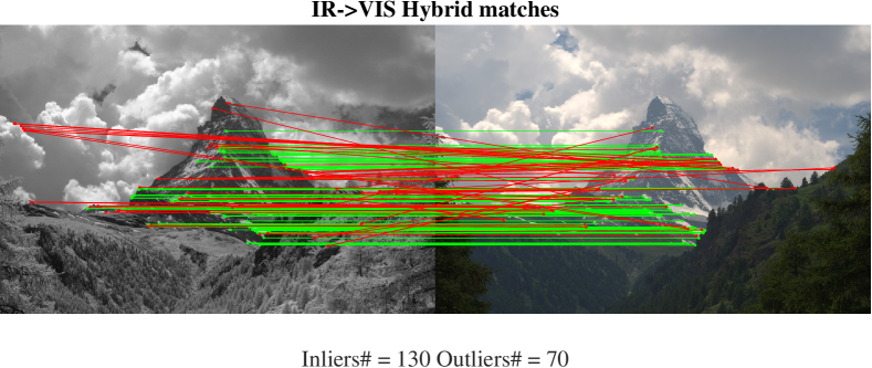
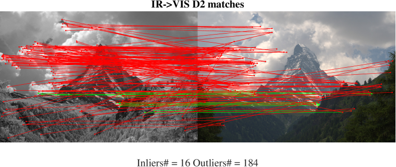
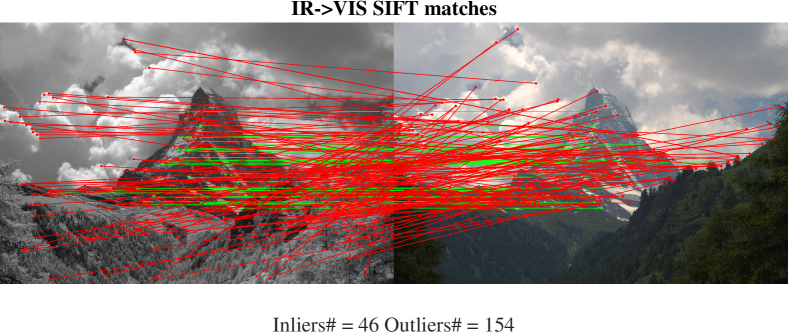
Figure 7: Qualitative feature detection and matching results. For each approach we match the top 200 detections in the IR image to top 400 detections in the VIS image, based on the $L_{2}$ distance of their descriptors. The inliers that are correctly matched within a $r=5$ are marked in green, while the outliers are marked in red.

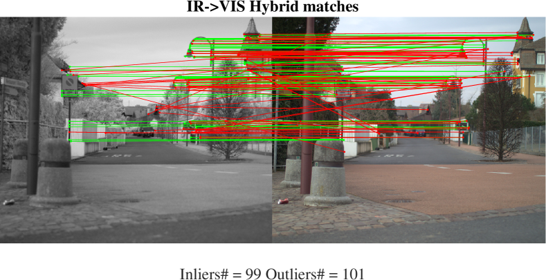
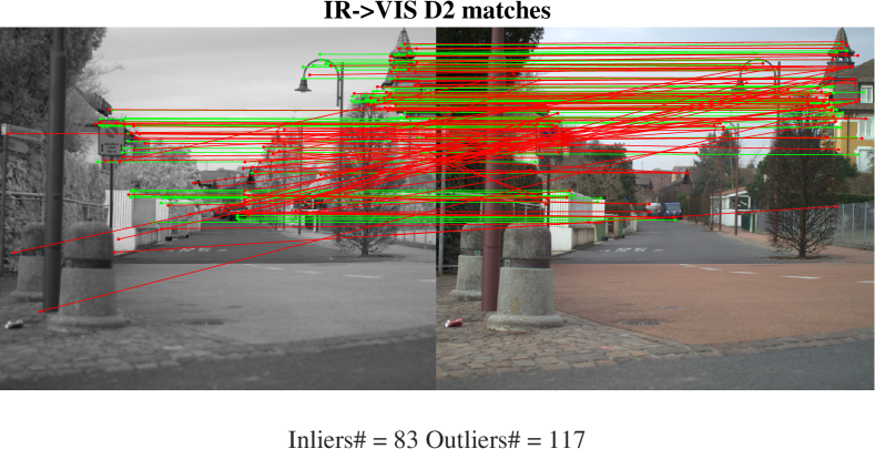
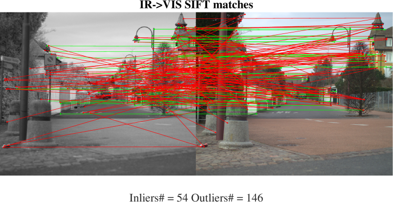
Figure 8: Qualitative feature detection and matching results. For each approach we match the top 200 detections in the IR image to top 400 detections in the VIS image, based on the $L_{2}$ distance of their descriptors. The inliers that are correctly matched within a $r=5$ are marked in green, while the outliers are marked in red.

4.5 Ablation study

We conducted an ablation study by comparing the results of the proposed Hybrid CNN to CNN formulations where one of the algorithmic components is omitted or changed. This allows to evaluate the contribution of each of the proposed components. Thus, we first compare to using only the Siamese and Asymmetric CNNs and also compare the results of training the Hybrid CNN using the multi-loss approach as in Section 3, to using a single loss ($L_{H}$ in Fig. 2) while omitting the auxiliary losses $L_{S}$ and $L_{A}$. We also show the added value of applying hard negative mining. The different CNNs were applied to the VIS-NIR [4] dataset using the experimental setup by En et al. [13], the same as in Section 4.3. The results are reported in Table V, where the Hybrid CNN is shown to outperform the Siamese and asymmetric CNNs when using either the CE or CL losses. The use of hardmining improves the accuracy significantly, for the CL-based results, in particular, by close to 6.5%. The auxiliary losses in the Hybrid scheme provides an additional accuracy improvement of 1.1%.

Network	Loss	#Losses	Hard Mining	VIS-NIR
Hybrid	CE	1	+	4.72
Symmetric	CE	1	+	4.2
Asymmetric	CE	1	+	5.8
Hybrid	CE	3	-	5.78
Hybrid	CE	3	+	3.66
Hybrid	CL	1	+	4.52
Symmetric	CL	1	+	9.56
Asymmetric	CL	1	+	4.32
Hybrid	CL	3	-	9.90
Hybrid	CL	3	+	3.41

TABLE V: Ablation results evaluated using the VIS-NIR dataset, where the patches were extracted using a uniform lattice layout as in En et al. [13]. The accuracy is given in terms of the FPR95 score. CE and CL relates to applying the Cross-Entropy and Contrastive losses, respectively. #Losses relates to the number of losses used for training. A single loss relates to training the CNN using a single loss $L_{H}$, as in Fig. 2.

5 Conclusions

In this work, we presented a Deep-Learning approach for the detection and matching of feature points in multimodal images, that utilizes a novel Hybrid CNN formulation consisting of two CNN sub-networks. The first is a Siamese (weight-sharing) CNN, while the second is an asymmetric (non-weigh-sharing) CNN. A novel feature points detection approach is derived by backtracking through the Siamese subnetwork activations, following the dominant activations. We show that the matching accuracy is improved by applying multi-loss learning to the Siamese and asymmetric sub-networks, alongside the principal output loss. The proposed scheme is experimentally shown to outperform state-of-the-art approaches when applied to multiple multimodal image datasets. It significantly reduces the matchings errors by two to threefold and outperforms state-of-the-art detectors such as SIFT, SURF and the D2-net in terms of detection repeatability.

References

- [1] Sameer Agarwal, Yasutaka Furukawa, Noah Snavely, Ian Simon, Brian Curless, Steven M Seitz, and Richard Szeliski. Building rome in a day. Communications of the ACM, 54(10):105–112, 2011.
- [2] C. A. Aguilera, A. D. Sappa, and R. Toledo. LGHD: A feature descriptor for matching across non-linear intensity variations. In 2015 IEEE International Conference on Image Processing (ICIP), pages 178–181, Sep. 2015.
- [3] Cristhian Aguilera, Fernando Barrera, Felipe Lumbreras, Angel D Sappa, and Ricardo Toledo. Multispectral image feature points. Sensors, 12(9):12661–12672, 2012.
- [4] Cristhian A. Aguilera, Francisco J. Aguilera, Angel D. Sappa, Cristhian Aguilera, and Ricardo Toledo. Learning cross-spectral similarity measures with deep convolutional neural networks. In The IEEE Conference on Computer Vision and Pattern Recognition (CVPR) Workshops, page 9. IEEE, Jun 2016.
- [5] Cristhian A Aguilera, Angel D Sappa, Cristhian Aguilera, and Ricardo Toledo. Cross-spectral local descriptors via quadruplet network. Sensors, 17(4):873, 2017.
- [6] Pablo Fernández Alcantarilla, Adrien Bartoli, and Andrew J. Davison. Kaze features. In Andrew Fitzgibbon, Svetlana Lazebnik, Pietro Perona, Yoichi Sato, and Cordelia Schmid, editors, Computer Vision – ECCV 2012, pages 214–227, Berlin, Heidelberg, 2012. Springer Berlin Heidelberg.
- [7] Herbert Bay, Andreas Ess, Tinne Tuytelaars, and Luc Van Gool. Speeded-up robust features (surf). Computer vision and image understanding, 110(3):346–359, 2008.
- [8] Andrei Z. Broder. Identifying and filtering near-duplicate documents. In Proceedings of the 11th Annual Symposium on Combinatorial Pattern Matching, COM ’00, pages 1–10, Berlin, Heidelberg, 2000. Springer-Verlag.
- [9] Matthew Brown and Sabine Süsstrunk. Multi-spectral SIFT for scene category recognition. In Computer Vision and Pattern Recognition (CVPR), 2011 IEEE Conference on, pages 177–184. IEEE, 2011.
- [10] Jian Chen and Jie Tian. Real-time multi-modal rigid registration based on a novel symmetric-SIFT descriptor. Progress in Natural Science, 19(5):643–651, 2009.
- [11] Christopher B Choy, JunYoung Gwak, Silvio Savarese, and Manmohan Chandraker. Universal correspondence network. In Advances in Neural Information Processing Systems, pages 2414–2422, 2016.
- [12] Mihai Dusmanu, Ignacio Rocco, Tomas Pajdla, Marc Pollefeys, Josef Sivic, Akihiko Torii, and Torsten Sattler. D2-net: A trainable cnn for joint detection and description of local features. In The IEEE Conference on Computer Vision and Pattern Recognition (CVPR), page 9. IEEE, Jun 2019.
- [13] S. En, A. Lechervy, and F. Jurie. TS-NET: Combining modality specific and common features for multimodal patch matching. In 2018 25th IEEE International Conference on Image Processing (ICIP), pages 3024–3028, Oct 2018.
- [14] Aristides Gionis, Piotr Indyk, and Rajeev Motwani. Similarity search in high dimensions via hashing. In Proceedings of the 25th International Conference on Very Large Data Bases, VLDB ’99, pages 518–529, San Francisco, CA, USA, 1999. Morgan Kaufmann Publishers Inc.
- [15] R. Hadsell, S. Chopra, and Y. LeCun. Dimensionality reduction by learning an invariant mapping. In 2006 IEEE Computer Society Conference on Computer Vision and Pattern Recognition (CVPR’06), volume 2, pages 1735–1742, 2006.
- [16] Mahmudul Hasan, Mark R Pickering, and Xiuping Jia. Modified SIFT for multi-modal remote sensing image registration. In Geoscience and Remote Sensing Symposium (IGARSS), 2012 IEEE International, pages 2348–2351. IEEE, 2012.
- [17] Md Tanvir Hossain, Guohua Lv, Shyh Wei Teng, Guojun Lu, and Martin Lackmann. Improved symmetric-SIFT for multi-modal image registration. In Digital Image Computing Techniques and Applications (DICTA), 2011 International Conference on, pages 197–202. IEEE, 2011.
- [18] Michal Irani and P Anandan. Robust multi-sensor image alignment. In Computer Vision, 1998. Sixth International Conference on, pages 959–966. IEEE, 1998.
- [19] Yosi Keller and Amir Averbuch. Multisensor image registration via implicit similarity. IEEE transactions on pattern analysis and machine intelligence, 28(5):794–801, 2006.
- [20] Seungryong Kim, Dongbo Min, Bumsub Ham, Seungchul Ryu, Minh N Do, and Kwanghoon Sohn. DASC: Dense adaptive self-correlation descriptor for multi-modal and multi-spectral correspondence. In Proceedings of the IEEE conference on computer vision and pattern recognition, pages 2103–2112, 2015.
- [21] Youngwook P Kwon, Hyojin Kim, Goran Konjevod, and Sara McMains. Dude (duality descriptor): A robust descriptor for disparate images using line segment duality. In Image Processing (ICIP), 2016 IEEE International Conference on, pages 310–314. IEEE, 2016.
- [22] S. Leutenegger, M. Chli, and R. Y. Siegwart. BRISK: Binary robust invariant scalable keypoints. In 2011 International Conference on Computer Vision, pages 2548–2555, Nov 2011.
- [23] Hui Li, BS Manjunath, and Sanjit K Mitra. A contour-based approach to multisensor image registration. IEEE transactions on image processing, 4(3):320–334, 1995.
- [24] Zhengqi Li and Noah Snavely. Megadepth: Learning single-view depth prediction from internet photos. In Computer Vision and Pattern Recognition (CVPR), 2018.
- [25] Tony Lindeberg. Detecting salient blob-like image structures and their scales with a scale-space primal sketch: A method for focus-of-attention. International Journal of Computer Vision, 11(3):283–318, Dec 1993.
- [26] David G Lowe. Distinctive image features from scale-invariant keypoints. International journal of computer vision, 60(2):91–110, 2004.
- [27] Rui Ma, Jian Chen, and Zhong Su. MI-SIFT: Mirror and inversion invariant generalization for SIFT descriptor. In Proceedings of the ACM International Conference on Image and Video Retrieval, CIVR ’10, pages 228–235, New York, NY, USA, 2010. ACM.
- [28] K. Mikolajczyk and C. Schmid. A performance evaluation of local descriptors. IEEE Transactions on Pattern Analysis and Machine Intelligence, 27(10):1615–1630, Oct 2005.
- [29] Anastasiya Mishchuk, Dmytro Mishkin, Filip Radenović, and Jiři Matas. Working hard to know your neighbor’s margins: Local descriptor learning loss. In Proceedings of the 31st International Conference on Neural Information Processing Systems, NIPS’17, pages 4829–4840, USA, 2017. Curran Associates Inc.
- [30] Dou Quan, Shuai Fang, Xuefeng Liang, Shuang Wang, and Licheng Jiao. Cross-spectral image patch matching by learning features of the spatially connected patches in a shared space. In C. V. Jawahar, Hongdong Li, Greg Mori, and Konrad Schindler, editors, Computer Vision – ACCV 2018, pages 115–130, Cham, 2019. Springer International Publishing.
- [31] Dou Quan, Xuefeng Liang, Shuang Wang, Shaowei Wei, Yanfeng Li, Ning Huyan, and Licheng Jiao. AFD-Net: Aggregated feature difference learning for cross-spectral image patch matching. In Proceedings of the 2019 International Conference on Computer Vision, ICCV ’19, Washington, DC, USA, 2019. IEEE Computer Society.
- [32] Sébastien Razakarivony and Frédéric Jurie. Vehicle detection in aerial imagery: A small target detection benchmark. Journal of Visual Communication and Image Representation, 34:187–203, 2016.
- [33] Ethan Rublee, Vincent Rabaud, Kurt Konolige, and Gary Bradski. ORB: An efficient alternative to SIFT or SURF. In Proceedings of the 2011 International Conference on Computer Vision, ICCV ’11, pages 2564–2571, Washington, DC, USA, 2011. IEEE Computer Society.
- [34] Eli Shechtman and Michal Irani. Matching local self-similarities across images and videos. In 2007 IEEE Conference on Computer Vision and Pattern Recognition, pages 1–8. IEEE, 2007.
- [35] O. Simeoni, Y. Avrithis, and O. Chum. Local features and visual words emerge in activations. In The IEEE Conference on Computer Vision and Pattern Recognition (CVPR), page 9. IEEE, Jun 2019.
- [36] Aristeidis Sotiras, Christos Davatzikos, and Nikos Paragios. Deformable medical image registration: A survey. IEEE transactions on medical imaging, 32(7):1153–1190, 2013.
- [37] Y. Tian, B. Fan, and F. Wu. L2-Net: Deep learning of discriminative patch descriptor in euclidean space. In 2017 IEEE Conference on Computer Vision and Pattern Recognition (CVPR), pages 6128–6136, July 2017.
- [38] Engin Tola, Vincent Lepetit, and Pascal Fua. Daisy: An efficient dense descriptor applied to wide-baseline stereo. IEEE transactions on pattern analysis and machine intelligence, 32(5):815–830, 2010.
- [39] Daniel Vaquero, Matthew Turk, Kari Pulli, Marius Tico, and Natasha Gelfand. A survey of image retargeting techniques. In Proc. SPIE, volume 7798, page 779814, 2010.
- [40] Paul Viola and William M. Wells, III. Alignment by maximization of mutual information. Int. J. Comput. Vision, 24(2):137–154, September 1997.
- [41] Shuang Wang, Yanfeng Li, Xuefeng Liang, Dou Quan, Bowu Yang, Shaowei Wei, and Licheng Jiao. Better and faster: Exponential loss for image patch matching. In The IEEE International Conference on Computer Vision (ICCV), October 2019.
- [42] Xiaogang Wang and Xiaoou Tang. Face photo-sketch synthesis and recognition. IEEE Transactions on Pattern Analysis and Machine Intelligence, 31(11):1955–1967, 2009.
- [43] Xufeng Han, T. Leung, Y. Jia, R. Sukthankar, and A. C. Berg. Matchnet: Unifying feature and metric learning for patch-based matching. In 2015 IEEE Conference on Computer Vision and Pattern Recognition (CVPR), pages 3279–3286, 2015.
- [44] Kwang Moo Yi, Eduard Trulls, Vincent Lepetit, and Pascal Fua. Lift: Learned invariant feature transform. In Bastian Leibe, Jiri Matas, Nicu Sebe, and Max Welling, editors, Computer Vision – ECCV 2016, pages 467–483, Cham, 2016. Springer International Publishing.
- [45] Sergey Zagoruyko and Nikos Komodakis. Learning to compare image patches via convolutional neural networks. In Proceedings of the IEEE Conference on Computer Vision and Pattern Recognition, pages 4353–4361, 2015.
- [46] Barbara Zitova and Jan Flusser. Image registration methods: a survey. Image and vision computing, 21(11):977–1000, 2003.