Two Thresholds for Globular Cluster Formation and their Dominance of Star Formation in the Early-Universe

Abstract

Young massive clusters (YMCs) are usually accompanied by lower-mass clusters and unbound stars with a total mass equal to several tens times the mass of the YMC. If this was also true when globular clusters (GCs) formed, then their cosmic density implies that most star formation before redshift $\sim 2$ made a GC that lasted until today. Star-forming regions had to change after this time for the modern universe to be making very few YMCs. Here we consider the conditions needed for the formation of a $\sim 10^{6}\;M_{\odot}$ cluster. These include a star formation rate inside each independent region that exceeds $\sim 1\;M_{\odot}$ yr^-1 to sample the cluster mass function up to such a high mass, and a star formation rate per unit area of $\Sigma_{\rm SFR}\sim 1\;M_{\odot}$ kpc^-2 yr^-1 to get the required high gas surface density from the Kennicutt-Schmidt relation, and therefore the required high pressure from the weight of the gas. High pressures are implied by the virial theorem at cluster densities. The ratio of these two quantities gives the area of a GC-forming region, $\sim 1$ kpc², and the young stellar mass converted to a cloud mass gives the typical gas surface density of $500-1000\;M_{\odot}$ pc^-2. Observations of star-forming clumps in young galaxies are consistent with these numbers, suggesting they formed today’s GCs. Observations of the cluster cut-off mass in local galaxies agree with the maximum mass calculated from $\Sigma_{\rm SFR}$. Metal-poor stellar populations in local dwarf irregular galaxies confirm the dominant role of GC formation in building their young disks.

1 Introduction

The globular clusters (GCs) that surround the Milky Way and most other galaxies formed when the universe was young, before a redshift of 1 to 2, in both metal-poor dwarf galaxies (Searle & Zinn, 1978; Zinnecker et al., 1988; Freeman, 1993) and less metal-poor disk galaxies (Kravtsov & Gnedin, 2005; Shapiro et al., 2010; Tonini, 2013; Rossi & Hurley, 2015), producing the two populations we observe today (Harris, 1991; Brodie & Strader, 2006; Bastian & Lardo, 2018). Many of the dwarfs were captured and dispersed by larger host galaxies, leaving their GCs in the host halos (Da Costa & Armandroff, 1995; Palma et al., 2002; Mackey & Gilmore, 2004; Gao et al., 2007; van den Bergh, 2007; Casetti-Dinescu, et al., 2009; Smith et al., 2009; Newberg et al., 2009; Mackey et al., 2010). Metal-rich globular clusters could have entered galaxy halos when interactions stirred up their disks (Kruijssen, 2015). The Sgr (Ibata et al., 1994) and Canis Major (Martin et al., 2004) dwarfs brought a dozen or more GCs to the Milky Way (Forbes & Bridges, 2010; Law & Majewski, 2010). Myeong et al. (2018) suggest 8 GCs came from another dwarf, and Kruijssen et al. (2018) suggest more came in earlier in a dwarf they call “Kraken.”

Tracing the origin of GCs is difficult because they were not bright enough when they formed to observe directly with present techniques. Gravitational lensing has revealed compact star-forming regions slightly more massive than GCs (Vanzella et al., 2017) and perhaps young GCs themselves (Johnson et al., 2017; Boylan-Kolchin, 2018). Lyman alpha emitting galaxies (Finkelstein et al., 2015; Zheng et al., 2017) may be a better source for finding GCs directly, as these galaxies can be observed in deep narrow-band Ly$\alpha$ surveys, their luminosities are consistent with star formation rates expected in GC-forming regions, and their luminosity function at low-mass gives the observed space density of today’s metal-poor GCs (Elmegreen et al., 2012). Dwarf galaxies in deep fields (“Little Blue Dots”) with extremely high specific star formation rates, $\sim 0.1$ Myr^-1 (star formation rate per unit stellar mass), are another possible source for metal-poor GCs (Elmegreen & Elmegreen, 2017a).

Globular cluster formation seems to be an important if not dominant mode of star formation in the early Universe. The space density of globular clusters today follows from the product of the average number per unit luminosity of their host galaxies and the number per unit volume of host galaxies with that luminosity. Portegies Zwart & McMillan (2000) derived 8 GCs Mpc^-3. For a $-2$ power law cluster mass function (Portegies Zwart et al., 2010), the total cluster mass associated with a most massive cluster of mass M_max is $M_{\rm max}\left(1+\ln(M_{\rm max}/M_{\rm min})\right)$ (Elmegreen et al., 2012) for minimum cluster mass $M_{\rm min}$. With an approximately 25% fraction of new stellar mass going into clusters (Chandar et al., 2017), the total stellar mass associated with a $10^{6}\;M_{\odot}$ cluster is $5\times 10^{7}\;M_{\odot}$, a factor of 50 mass multiplier (weakly dependent on $M_{\rm min}$, which was assumed to be $100\;M_{\odot}$ from Lada & Lada, 2003). If these $10^{6}\;M_{\odot}$ clusters are the 8 Mpc^-3 GCs around today, then the stellar density from their formation is $4\times 10^{8}\;M_{\odot}$ Mpc^-3. This is the same as the average co-moving stellar density in the universe at a redshift of around 1 in the compilation by Madau & Dickinson (2014). Boylan-Kolchin (2018) similarly derive a major contribution by GCs to the high-redshift galaxy luminosity function at the low end. If the space density of metal-poor GCs is $\sim 2$ Mpc^-3, as estimated by Boylan-Kolchin (2017) using the correlation between GCs and dark matter halos, then the associated stellar density is about half the above value, considering also the metal-rich GCs that formed later. Evidently, a high fraction of star-forming regions included at least one globular cluster before about half the age of the universe.

A similar calculation illustrates the importance of GC formation to the universal star formation rate at early times. If we consider that the duration of the star formation event which made a GC was $\Delta t$, and the redshift range over which they formed was from $z=7$ to 2, a period of 2.6 Gyr, then the average star formation rate from GC-forming events with $M_{\rm max}\sim 10^{6}\;M_{\odot}$ is ($5\times 10^{7}\;M_{\odot}/\Delta t)\times(\Delta t/2.6\;{\rm Gyr})\times(8\;{\rm Mpc}^{-3})$, where the second term is the fraction of time each event occupies in the GC-forming era. The resultant average associated star formation rate is $0.15\;M_{\odot}$ yr^-1 Mpc^-3, which is the same as the peak value of the co-moving cosmic star formation rate density in the universe that occurs at redshift $\sim 2$ (Madau & Dickinson, 2014).

These two calculations suggest that the early universe was filled with star-forming regions containing young massive clusters that ended up as today’s GCs. There was little additional star formation making smaller clusters or OB associations that dispersed, aside from the smaller clusters and associations directly connected with the GCs. Today the mass density of GC stars is their space density times their average mass of $\sim 2\times 10^{5}\;M\odot$ (Harris, 2001), or $1.6\times 10^{6}\;M_{\odot}$ Mpc^-3. This is 0.26% of the current total stellar mass density from Madau & Dickinson (2014), a factor of $\sim 1/380$. The first factor of 50 in this 380 is presumably from scattered stars that formed with the GCs, and then the remaining factor of $\sim 8$ would be from stars that formed recently without making massive clusters.

We can also learn about early star formation in dwarf galaxies from their old stellar populations. WLM has an old metal-poor GC whose luminosity suggests it contains $\sim 10^{6}\;M_{\odot}$ of stars (Elmegreen et al., 2012). The mass of other stars at the same age and metallicity is comparable to this (Leaman et al., 2012; Larsen et al., 2014), suggesting the GC was a high fraction of the total WLM mass when it formed (Elmegreen et al., 2012). Similarly, the GC mass in the Fornax dwarf spheroidal was $\sim 0.25$ of the galaxy stellar mass when the GC formed (Larsen et al., 2012). For IKN and NGC 147, these fractions are $\sim 0.5$ and $0.06$, respectively (Larsen et al., 2014, 2018). These are enormously high fractions, especially considering the additional cluster mass that might have been present in the full cluster mass function. Perhaps the clustered fraction of stars at birth was larger than the 25% assumed above, even close to 100% as suggested by Messa et al. (2018) for regions with high star formation rate densities. In either case, the star formation events that formed the observed GCs also made most of the stellar disks at the same time. These were whole-galaxy starbursts.

The specific frequency of GCs in local dwarf galaxies also suggests nearly the whole galaxy was involved in the same starburst. The number of GCs per $10^{9}\;M_{\odot}$ of stars is $\sim 100$ for a stellar mass today of $3\times 10^{8}\;M_{\odot}$ (Zaritsky et al., 2016). Multiplying the number of GCs by their current average mass, $\sim 2\times 10^{5}\;M_{\odot}$, gives a current mass fraction of 2%. At 10% of the age of the universe these GCs were there but the stellar mass was only about one-tenth as much, making the GC mass fraction $\sim 20$% in the dwarf galaxies. For more massive initial GCs, i.e., considering evaporation and an escaped population of first-generation stars that contributed p-processed elements to approximately half of the remaining stars (Bastian & Lardo, 2018), and considering also the accompanying star formation in the same burst, the GC mass fraction gets close to $\sim 100$%.

The Milky Way has a relatively low total mass of stellar streams and halo stars accompanying its GCs. Observations by Martell et al. (2016) of Milky Way halo stars with metallicities matching those of the second generation in GCs (e.g., high Nitrogen) suggest only an equivalent mass of these stars in the halo. This equivalence suggests GC evaporation halved their initial mass (see also Vesperini, 1998). More important for the present discussion are the stars accompanying the first generation in each GC, which outnumber the GC stars by a factor of $\sim 20$ in the halo (Martell, 2017). These stars presumably come from the environment in which the GCs formed, including those in the GC-forming event prior to self-enrichment or some other process (Bastian & Lardo, 2018). While this factor of 20 is more than enough to allow the first generation stars in each GC to enrich the second generation and mostly escape into the halo (Bastian & Lardo, 2018), it is not enough to carry along with each GC a significant mass of other stars in an associated dwarf galaxy. Sollima & Baumgardt (2017) inferred an even higher fractional mass loss from Milky Way GCs using the mass distribution functions of remaining stars, whose shape correlates with the mass loss fraction. They suggest $2\times 10^{8}\;M_{\odot}$ of stars escaped from GCs, compared to $\sim 10^{9}\;M_{\odot}$ in the halo (Morrison, 1993; Bell et al., 2008; Deason et al., 2011). These escaped stars are so numerous that they leave little room for additional stellar mass in accompanying dwarf galaxies. This requires that most of the dwarf galaxies that brought in metal-poor GCs were accreted so early that they were still dominated by their GC-forming population.

Local dwarf galaxies rarely form clusters as massive as a globular cluster (Billett et al., 2002; Larsen, 2009) and they never have nearly all of their stellar mass resulting from a single burst. NGC 1569 (Stil & Israel, 1998) and NGC 5253 (López-Sánchez et al., 2012; Turner et al., 2015; Miura et al., 2015) have YMCs, but these clusters contain only 0.1% of the galaxy stellar masses (De Marchi et al., 1997; Johnson et al., 2012; Sabbi et al., 2018; Calzetti et al., 2015). The origin of these YMCs may be related to impacting gas streams, which are present in both cases. Most local starburst dwarfs have lopsided HI (Lelli et al., 2014). A major gas impact is suspected also in the dwarf “tadpole” galaxy Kiso 5639, which has a molecular cloud at one end with a gas mass comparable to the total stellar mass in the whole disk, and is currently forming 14 young star clusters more massive than $10^{4}\;M_{\odot}$ (Elmegreen et al., 2016, 2018). Mrk 930 is another starburst dwarf with a high formation efficiency for clusters (Adamo et al., 2011) and NGC 1705 has a YMC with no evidence for an impact or merger. YMC formation in major mergers of large galaxies is more common (Whitmore et al., 2010).

Clearly there was a transition at around redshift 1 to 2 from conditions that made $10^{6}\;M_{\odot}$ clusters in most star-forming regions of the early universe to present-day conditions that rarely make them except perhaps in major mergers. We investigate this transition here, suggesting it is almost entirely the result of a higher gas surface density at that time. Observations show this high surface density directly (e.g., Tacconi et al., 2018; Cava et al., 2018), so the result may not be surprising. There are few observation yet for the origin of this high surface density, but the usual explanations of enhanced cold accretion (e.g., Inoue et al., 2016) and galaxy mergers (e.g., Yozin & Bekki, 2012; Kim et al., 2018), are both likely contributors.

An implicit assumption in this paper is that the basic star formation processes at the redshifts where GCs formed were the same as they are in galaxies today. These processes involve gaseous gravity and cooling, as mitigated and partitioned by hydromagnetic turbulence and star formation feedback (McKee & Ostriker, 2007; Krumholz et al., 2018). As a result, the cluster mass function at birth and the concurrent formation of clustered and non-clustered stars are probably similar then and now too. Other possible assumptions such as a top-heavy cluster mass function at high redshift are not necessary in the present model.

In what follows, Section 2 derives the minimum star formation rate to sample the cluster mass function up to a GC-forming mass of $\sim 10^{6}\;M_{\odot}$. The result, $\sim 1\;M_{\odot}$ yr^-1, is commonly observed in today’s galaxies but typically spread out over a disk spanning many kpc², which corresponds to too low an areal rate and too low a pressure to make a GC in any local region. This leads to a second condition in Section 3, which is that the surface density of star formation has to exceed $\sim 1\;M_{\odot}$ pc^-2 Myr^-1 for the local pressure to compact the required amount of mass up to the density of a star cluster. These two relations suggest that $\sim 1$ kpc is the characteristic size of a GC-forming region and the minimum size of a GC-forming galaxy (on average). The second condition also corresponds to the observed cut-off mass in the local cluster mass function. This cut-off mass is predicted to be difficult to observe unless the product of the surface area and the duration of star formation is fairly large, because for a small value of this combined parameter, the maximum mass that is likely to be observed from the sample size is only comparable to or smaller than the cut-off mass (Sect. 4). A brief comparison of these two thresholds to observations of star formation at high redshift is in Section 5. This comparison implies that approximately half of the star-formation in giant clumps has the required local star formation rate and density to make a $10^{6}\;M_{\odot}$ cluster, which supports the above suggestion that GCs and their associated stars were pervasive in the early universe.

2 Minimum star formation rate

An important condition for the formation of a YMC is a high star formation rate, so the cluster mass function, which is presumably from a random distribution of clump masses in a turbulent, self-gravitating gas, can be sampled far out into the high-mass tail where turbulent structures are rare. Assuming this mass function is a Schechter function with a power law slope of $-2$ and a cutoff mass $M_{\rm c}$ (Gieles et al., 2006a, b; Jordán et al., 2007; Bastian et al., 2012; Adamo et al., 2015), i.e.,

$$dn(M)/dM=n_{0}M^{-2}\exp(-M/M_{\rm c}),$$ (1)

the maximum likely mass $M_{\rm max}$ is given by the condition that there is one cluster at or larger than that mass,

$$\int_{M_{\rm max}}^{\infty}n(M)dM=1,$$ (2)

which defines $n_{0}(M_{\rm max})$ . The total mass in all clusters is then

$$M_{\rm cl,total}(M_{\rm max})={{\int_{M_{\rm min}}^{\infty}M(dn[M]/dM)dM}\over{\int_{M_{\rm max}}^{\infty}(dn[M]/dM)dM}}$$ (3)

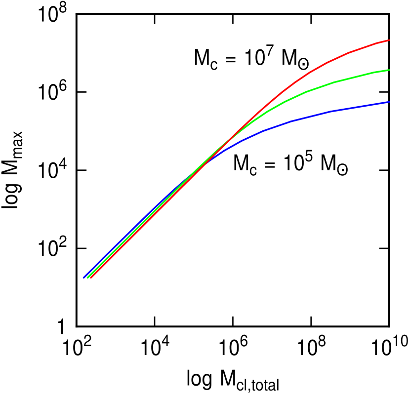
Figure 1: The maximum likely mass of a star cluster as a function of the total mass in clustered stars for three Schechter mass functions with different cut-off masses. For the assumed $-2$ power law in the mass function, the maximum likely cluster mass increases linearly with the total clustered mass up to the cut-off mass, and then the total mass has to increase more rapidly to get much of an increase in the maximum mass.

where $M_{\rm min}$ is the minimum cluster mass. This equation can be solved to give the maximum likely cluster mass as a function of the total cluster mass for each value of $M_{\rm c}$. Figure 1 shows the result for the function given by equation (1). For $M_{\rm c}\sim 10^{5}\;M_{\odot}$ as in local galaxies (Gieles et al., 2006a; Adamo et al., 2015, 2017; Messa et al., 2017; Johnson et al., 2017), the total cluster mass in the starburst has to be comparable to the mass of stars in a Milky Way size galaxy before a $\sim 10^{6}\;M_{\odot}$ cluster is expected, and this is not realistic. The formation of a young GC with this mass in a dwarf galaxy requires a high M${}_{\rm c}\geq 10^{7}\;M_{\odot}$, so the mass function up to the GC mass is effectively a pure power law. Then the expression for total cluster mass is integrated to give

$$M_{\rm cl,total}=M_{\rm max}\left(1+\ln\left[{{M_{\rm max}}\over{M_{\rm min}}}\right]\right).$$ (4)

(In the numerator of equation 3, the partial integral over mass from $M_{\rm max}$ to infinity was set equal to M_max to avoid a divergence in the logarithm of infinity). If a fraction $\Gamma$ of stars form in clusters according to this mass function and the rest are dispersed, then the total stellar mass in the starburst event is $M_{\rm cl,total}/\Gamma$.

Equation 4 suggests that the total young stellar mass associated with a $\sim 10^{6}\;M_{\odot}$ cluster is $5\times 10^{7}\;M_{\odot}$ for $\Gamma\sim 0.25$ (Adamo et al., 2011; Chandar et al., 2017) and $M_{\rm min}\sim 100\;M_{\odot}$. This mass should be divided by the duration of star formation to get the average star formation rate. The duration of star formation, $\Delta t$, is typically a crossing time in a gravitating, turbulent region. For a giant clump in a disk galaxy or a whole dwarf galaxy, the physical size might be $\sim 1$ kpc and the velocity dispersion $\sim 20$ km s^-1, giving a characteristic timescale for the starburst equal to $\Delta t\sim 50$ Myr. Then the star formation rate is $\sim 1\;M_{\odot}$ yr^-1. The same duration results if we consider a total efficiency of star formation equal to $2.5$% and a gas consumption time of $\sim 2$ Gyr (e.g., Krumholz & Tan, 2007; Bigiel et al., 2008).

The uncertainty in $\Gamma$ at high and low redshift and the lack of observations of the cluster mass function at high redshift limit the precise application of this minimum star formation rate. However, variations in $\Gamma$ are likely to be only a factor of a few, since it cannot be larger than 1, and the power law in the cluster mass function seems to be a fundamental property of hierarchical fragmentation (Fleck, 1996; Elmegreen & Efremov, 1997), so variations in that are also likely to be small. In what follows, we continue to use $\Gamma\sim 0.25$ as representative during the epoch of GC formation. It enters only in the minimum star formation rate derived here and not the minimum star formation rate surface density considered in Section 3.

The results suggest that a region of star formation the size of a dwarf galaxy or a giant clump in a larger clumpy galaxy (Sect. 5),forming stars at a rate, $S$, of at least $\sim 1\;M_{\odot}$ yr^-1 for $\sim 50$ Myr, should form at least one $10^{6}\;M_{\odot}$ cluster that can be a possible predecessor to a GC. We write this result as

$$M_{\rm max,SOS}\sim 10^{6}\;M_{\odot}\left({S\over{1\;M_{\odot}\;{\rm yr}^{-1}}}\right)\left({{\Delta t}\over{50\;{\rm Myr}}}\right),$$ (5)

where ‘SOS’ refers to the Size of Sample effect, which was the basis for deriving this mass. There is also a small logarithmic dependence on this maximum mass (eq. 4) that has been ignored in this equation (i.e., $1+\ln(M_{\rm max}/M_{\rm min})$ was set equal to 12.5).

As an example, consider the two local dwarf starburst galaxies where this magnitude of star formation is associated with YMCs. The starburst in NGC 1569 made three clusters of mass $3.9\times 10^{5}\;M_{\odot}$, $4.4\times 10^{5}\;M_{\odot}$, and $2.3\times 10^{5}\;M_{\odot}$ (Gilbert & Graham, 2002, see also De Marchi et al. 1997, Larsen et al. 2011), and the star formation rate in that region is $\sim 1\;M_{\odot}$ yr^-1 depending on the assumed initial stellar mass function (Greggio et al., 1998). Also for NGC 5253 with two clusters of mass $7.5\times 10^{4}\;M_{\odot}$ and $2.5\times 10^{5}\;M_{\odot}$, the star formation rate is $0.4\;M_{\odot}$ yr^-1 over a timescale of $\sim 10$ Myr (Calzetti et al., 2015).

Statistical sampling suggests that a galaxy with 10 regions of star formation having a rate of $0.1\;M_{\odot}$ yr^-1 each should have the same probability of forming a $10^{6}\;M_{\odot}$ cluster as a single region with $10\times$ the rate. This is not the case in fact because the maximum mass of a cluster depends on the pressure through the $M_{\rm c}$ in the Schechter function, and the pressure depends on the star formation rate per unit area, not just the total rate. This additional dependence will be discussed in the next section. The statistical sampling argument, in which the maximum cluster mass is proportional to the number or total luminosity of clusters with the same age (Larsen, 2002; Randriamanakoto et al., 2013; Kruijssen & Cooper, 2012; Whitmore et al., 2014), should work in principle even if each star-forming region is independent, because the large regions themselves should have a range of masses that follow a power law function, as shown in Section 5. Galaxies with total star formation rates of several $M_{\odot}$ yr^-1 like the Milky Way and local spirals do not form $10^{6}\;M_{\odot}$ clusters because each independent region has too low a pressure. We discuss in section 4 how the maximum cluster mass from pressure considerations compares with the maximum cluster mass from the size-of-sample effect.

3 Minimum star formation surface density

3.1 Minimum Pressure

Massive clusters need high pressure environments to produce the high stellar densities and masses of the gravitating cloud cores in which they form (Elmegreen & Efremov, 1997), and to offset the effects of young stellar feedback (Kruijssen, 2012). The most direct way to see this is from the virial theorem, which can be used to relate the mass of a self-gravitating cloud to the pressure and density:

$$M_{\rm cloud}=(2\pi)^{3/2}(3/4\pi)^{2}(P_{\rm cloud}/G)^{3/2}\rho_{\rm cloud}^{-2}.$$ (6)

This comes from the equations $P=(\pi/2)G\Sigma^{2}$, $\Sigma=M/(\pi R^{2})$, and $M=(4\pi/3)\rho R^{3}$ for average cloud surface density $\Sigma$ and radius $R$. Setting $M_{\rm cluster}=\epsilon_{\rm M}M_{\rm cloud}$ and $\rho_{\rm cluster}=\epsilon_{\rm\rho}\rho_{\rm cloud}$ for efficiencies in the gravitating region equal to $\epsilon_{\rm M}$ and $\epsilon_{\rm\rho}$, and combining these into a single parameter $\epsilon=\epsilon_{\rm M}\epsilon_{\rm\rho}^{2}$,

$$M_{\rm cluster}=0.9\epsilon(P_{\rm cloud}/G)^{3/2}\rho_{\rm cluster}^{-2}.$$ (7)

Note that for a given pressure, more massive gravitating regions can form if the density is lower. Thus OB associations, which have relatively low density, can be more massive than bound clusters at a given pressure.

Inverting equation (7),

$$P_{\rm cloud}=G\left(1.1M_{\rm cluster}\rho_{\rm cluster}^{2}/\epsilon\right)^{2/3}.$$ (8)

For a cluster with $M_{\rm cluster}=10^{6}\;M_{\odot}$ inside a half-mass radius of $\sim 3$ pc, the stellar density is $\rho_{\rm cluster}\sim 0.9\times 10^{4}\;M_{\odot}$ pc^-3. Setting $\rho_{\rm cluster}=10^{4}\;M_{\odot}$ pc^-3 and $\epsilon=0.5$ for the core of the cloud, equation (8) gives $P_{\rm cloud}\sim 8\times 10^{10}k_{\rm B}$ for Boltzman’s constant $k_{\rm B}$. For 8 YMCs in Bastian et al. (2014), the average stellar density determined from the ratio of the photometric mass to the volume at the effective radius is $\sim 10^{5}\;M_{\odot}$ pc^-3 and then the average pressure from equation (8), considering also the cluster masses, is $P_{\rm cloud}\sim 2\times 10^{12}k_{\rm B}$. For comparison, the typical pressure in the cluster-forming core of a Milky Way cloud, such as the Orion cloud, is much lower, $5\times 10^{7}$k_B from the average of 7 regions observed by Lada et al. (1997). The cluster masses are much lower in Orion too. The average gas density in these Orion regions is $3\times 10^{5}$ cm^-3 and the average one-dimensional velocity dispersion is $\sim 0.8$ km s^-1, which combine to give the pressure.

Observed cluster densities like that in Orion may not be appropriate for equation (8), which assumes a static virialized cloud core. If gas continuously streams into a core and forms stars, then the true stellar density can be larger than $\epsilon_{\rho}$ times the virialized gas density at pressure $P_{\rm cloud}$. This is the conveyer belt model of Longmore et al. (2014) and Walker et al. (2016). The effect is to lower the required gas pressure to get a cluster of a certain stellar density. Effectively, $\epsilon>1$ in this case. For the following discussion, we assume $P_{\rm cloud}\sim 10^{11}k_{\rm B}$ as representative for $M_{\rm cluster}=10^{6}\;M_{\odot}$. Then $\epsilon\sim 0.4$ as above if $\rho_{\rm cluster}\sim 10^{4}\;M_{\odot}$ pc^-3; $\epsilon$ increases as the square of $\rho_{\rm cluster}$ in the conveyer belt model for the same cluster mass and cloud pressure.

Equation (8) is based on self-gravitational binding and not feedback. The role of feedback in limiting the mass of a cluster is not clear. Ginsburg et al. (2016) suggest that feedback has virtually no role and gas exhaustion stops star formation in the cluster, rather than gas expulsion (see also Girichidis et al., 2012; Kruijssen, 2012; Matzner, 2017; Galván-Madrid et al., 2017; Tsang & Milosavljević, 2018; Silich & Tenorio-Tagle, 2018; Cohen et al., 2018; Ward & Kruijssen, 2018). Also, there is no jump in the mass function of bound clusters at a mass of around $10^{3}\;M_{\odot}$ where ionization feedback suddenly increases as a result of the increasingly likely appearance of O-type stars (Vacca et al., 1996). If gas expulsion from young stellar feedback was critical in limiting the boundedness of a cluster, then the probability that a cluster ends up bound should drop suddenly when feedback from O-type stars spikes upward, causing a comparable drop in the bound cluster mass function. However this is not observed (e.g., Bressert et al., 2010). Possibly, feedback affects loosely bound clouds (Kruijssen, 2012; Matzner & Jumper, 2015). Various types of feedback and their relative roles in cloud core dispersal were discussed in Krumholz et al. (2018).

The cluster mass dependence in equation (8) has not been written fully yet. Most likely, cluster radius varies weakly with mass (Ryon et al., 2017) and cluster density varies more strongly. In Section 3.3 we consider that radius increases approximately as $M^{0.11}$ and $\rho_{\rm cluster}\propto M^{0.66}$. Then $P_{\rm cloud}\propto M_{\rm cluster}^{1.5}$ from equation (8).

3.2 Conversion from Cloud Core Pressure to Galaxy Gas Surface Density

High pressure in an equilibrium disk requires a high gas surface density, or actually, a high product of the gas surface density, $\Sigma_{\rm gas}$, and the total surface density, $\Sigma_{\rm total,GL}$, from the sum of the gas, stars and dark matter inside the gas layer (subscript ’GL’), which all contribute to the gravity that weighs down the gas. The resulting pressure is only partly in the form of turbulent gas motions, which contribute to the core pressure and density inside a cluster-forming cloud, because other parts of the total pressure are from magnetic fields and cosmic rays, which resist the weight of the gas too. We let the turbulent fraction of the pressure be $\zeta\sim 0.3$ considering equipartition with the other types (Boulares & Cox, 1990).

For a young galaxy with a high gas fraction, $\Sigma_{\rm gas}\sim 0.5\Sigma_{\rm total,GL}$. For a modern galaxy with a gas disk much thinner than the stellar disk and the dark matter spheroid, the coefficient is only a little smaller. For example, in the solar neighborhood, the total stellar midplane density is $0.043\pm 0.04\;M_{\odot}$ pc^-3 and the gas density is $1.17$ cm^-3, equivalent to $0.041\pm 0.004\;M_{\odot}$ pc^-3; dark matter adds another $0.013\pm 0.003\;M_{\odot}$ pc^-3 (McKee et al., 2015). Thus locally, $\Sigma_{\rm gas}\sim 0.4\Sigma_{\rm total,GL}$. We set $\Sigma_{\rm gas}\sim\xi\Sigma_{\rm total,GL}$ for the following discussion but because the gas is a little more concentrated to the midplane than the stars, assume $\xi\sim 0.3$ for numerical evaluations.

The general equation for total pressure in a disk is (Elmegreen, 1989),

$$P_{\rm total}=(\pi/2)G\Sigma_{\rm gas}\Sigma_{\rm total,GL}$$ (9)

which comes from $P=\rho\sigma^{2}(1+\alpha+\beta)$ with gas density $\rho=\Sigma/(2H)$ and scale height $H=\sigma^{2}(1+\alpha+\beta)/(\pi G\Sigma_{\rm total,GL})$ for velocity dispersion $\sigma$, magnetic pressure $\alpha\rho\sigma^{2}$, and cosmic ray pressure, $\beta\rho\sigma^{2}$. Note that $\alpha$ and $\beta$ cancel from equation (9).

For the cloud pressure, we consider only the turbulent component of the interstellar pressure, writing $P_{\rm ISM,turb}=\zeta P_{\rm total}$ from above, and total surface density, $\Sigma_{\rm total,GL}=\Sigma_{\rm gas}/\xi$ to derive

$$P_{\rm ISM,turb}={{\pi\zeta}\over{2\xi}}G\Sigma_{\rm gas}^{2}.$$ (10)

where $\zeta/\xi\sim 1$ (i.e., the additional compression from stars and dark matter approximately balances the additional expansion from magnetic fields and cosmic rays).

Equation (10) is a first step to estimate the minimum gas surface density in an equilibrium region of a disk that forms a YMC. What we need is the cloud core pressure, which is used in equation (8). This core pressure, $P_{\rm cloud}$, is much larger than the average interstellar turbulent pressure $P_{\rm ISM,turb}$ because of the additional weight of the cloud envelop pressing down on the core. We assume these two pressures are proportional to each other and write $P_{\rm cloud}=CP_{\rm ISM,turb}$ where $C$ is a compaction factor that could be several orders of magnitude, as estimated below. With this, equations (8) and (10) combine to give

$$\Sigma_{\rm gas}=\left({{2\xi}\over{\pi C\zeta}}\right)^{1/2}\left({{1.1M_{\rm cluster}\rho_{\rm cluster}^{2}}\over{\epsilon}}\right)^{1/3}=1.0\left({\xi\over{C\zeta}}\right)^{1/2}\epsilon^{-1/3}\Sigma_{\rm cluster}.$$ (11)

Here we have used $M_{\rm cluster}=\Sigma_{\rm cluster}\pi R_{\rm cluster}^{2}$ and $\rho_{\rm cluster}=3\Sigma_{\rm cluster}/(4R_{\rm cluster})$ for cluster stellar surface density $\Sigma_{\rm cluster}$. With fiducial values of $M_{\rm cluster}=10^{6}\;M_{\odot}$, $\rho_{\rm cluster}=10^{4}\;M_{\odot}$ pc^-3, $\xi/\zeta=1$, and $\epsilon=0.5$, the average interstellar surface density should satisfy $\Sigma_{\rm gas}C^{1/2}=4.8\times 10^{4}\;M_{\odot}$ pc^-2. This result is consistent with the peak stellar surface densities in YMCs compiled by Walker et al. (2016), considering the second expression in equation (11). Walker et al. (2016) find that typical YMCs in the Milky Way have $\Sigma_{\rm cluster}\sim 1.3\times 10^{4}\;M_{\odot}$ pc^-2.

Now we evaluate $C$. This compaction factor comes from the density stratification inside molecular clouds. We consider that density varies approximately as a power law with radius in a spherical cloud, $\rho\propto R^{-\kappa}$, as expected from self-gravity in either isothermal equilibrium ($\kappa=2$) or collapse ($\kappa=1.5$) conditions (Shu, 1977; Murray & Chang, 2015). Observations show profiles like this in individual clouds (Mueller et al., 2002) but they may also be inferred from the high-density power-law part of the column density probability distribution functions (N-PDF) in cloud surveys. Corbelli et al. (2018) determined this distribution function for molecular clouds in M33 and found in two large regions an N-PDF slope of around $-2$. Lin et al. (2017) observed an N-PDF slope change from $-4$ to $-2$ in Milky Way dark clouds as the luminosity-to-mass ratio increased. For active regions of YMC formation, the luminosity-to-mass ratio will be high and we might expect an N-PDF slope of $\sim-2$. This corresponds to $\kappa\sim 2$ using the relation $\kappa=1+2/p$ for N-PDF slope $-p$ (Elmegreen, 2018). If cloud internal density varies with radius as $R^{-2}$, then the cloud surface density varies as $R\rho(R)\propto R^{-1}$, and the cloud pressure, which scales with the square of the surface density, varies as $(R\rho(R))^{2}\propto R^{-2}$. In summary, an N-PDF with a slope of $-p$ on a log-log plot suggests an internal radial variation of column density inside self-gravitating cloud that has a power law slope of $-2/p$ and a pressure variation with radius proportional to $R^{-4/p}$.

This type of dependence makes sense as an approximation if we consider a local giant molecular cloud like Orion using $p\sim 2$. The average local total ISM pressure on the scale of the molecular disk thickness, 100 pc (Heyer & Dame, 2015), is $\sim 2.8\times 10^{4}k_{\rm B}$ of which about $1/3$ is turbulent (Boulares & Cox, 1990), making $P_{\rm ISM,turb}\sim 10^{4}$k_B. The pressure inside the cluster-forming core is about a factor of $10^{4}$ higher, $\sim 10^{8}k_{\rm B}$, as given above, and the corresponding spatial scale is a factor of $\sim 10^{2}$ smaller, $\sim 1$ pc. Thus average pressure scales about as the inverse square of size, zooming into the Orion core.

A key assumption here is that molecular clouds like Orion are the densest parts of a self-gravitating interstellar medium, i.e., with Toomre $Q$ close to 1, and that the surrounding dark and atomic gas continues to be stratified up to the disk thickness because this lower-density gas is also part of the total interstellar gravity (Elmegreen & Elmegreen, 1987; Grabelsky et al., 1987; Elmegreen et al., 2018). This juxtaposition of CO clouds inside larger HI clouds has been observed in nearby galaxies (Lada et al., 1988; Corbelli et al., 2018).

The scaling of pressure with radius inside individual clouds is not easily evaluated from cloud surveys. Consider the $\sim 1100$ CO-emitting clouds in the Rice et al. (2016) catalog that have unambiguous distances. The average radius of these clouds is $34\pm 23$ pc, the average log of the surface density (calculated as the total cloud mass divided by the area) is $1.37\pm 0.43$ in units of $M_{\odot}$ pc² (i.e., the surface density itself is $\sim 23\;M_{\odot}$ pc^-2), and the average log of the pressure (calculated as the product of the average density and the square of the velocity dispersion) is $4.1\pm 0.7$ in units of $k_{\rm B}$. Many of these clouds are not gravitating, however, so their pressures are not particularly high. For the $\sim 400$ clouds that are self-gravitating, with virial parameter $\alpha<2$, the average log pressure is $4.3\pm 0.8$, which is about twice the ambient turbulent pressure. We should consider also the decrease in pressure and cloud surface density with galacto-centric radius (Heyer & Dame, 2015). If we just consider the 173 GMCs near the solar position, with galactocentric radii between 8 and 9 kpc (for the Sun at 8.5 kpc), then the average GMC radius is $22\pm 11$ pc, the average log of the surface density is $1.70\pm 0.32$ in $M_{\odot}$ pc^-2 ($50\;M_{\odot}$ pc^-2), and the average log of the pressure is $4.7\pm 0.5$ in $k_{\rm B}$. These local numbers suggest a scaling of turbulent cloud pressure with the inverse first power of the size, i.e., the average cloud is $\sim 5$ times smaller than the disk scale height and $\sim 5$ times higher in pressure than average. If we narrowly confine the sample to the solar neighborhood with low $\alpha$ and a limited mass range, e.g., from $10^{4}\;M_{\odot}$ to $10^{5}\;M_{\odot}$, then the pressure scales as approximately the inverse 4th power of size, following equation (6).

A better evaluation of the ratio $C$ of the typical cluster-forming core pressure to the average interstellar turbulent pressure would seem to come from the power-law N-PDFs observed by Druard et al. (2014) and Corbelli et al. (2018), which are for galactic-scale regions in M33, and for Milky Way clouds observed by (Lin et al., 2017), which both suggest an average power law slope of around $-2$. This corresponds to an inverse square radial dependence for density in individual clouds. Thus it is reasonable to expect that the pressure in a parsec-size cloud core that forms a YMC is around $C\sim 10^{4}$ times the average ISM turbulent pressure on the $\sim 100$ pc scale of the disk thickness. We assume this value of $C$ in what follows, even for thicker disks and proportionally bigger cloud cores at high redshift, because the higher turbulent speeds then (Förster-Schreiber et al., 2009) should increase the sizes of all self-gravitating regions in proportion to each other. Now equation (11) becomes

$$\Sigma_{\rm gas}\sim 8.2\times 10^{-3}\left({{M_{\rm cluster}\rho_{\rm cluster}^{2}}\over{\epsilon}}\right)^{1/3}=0.01\epsilon^{-1/3}\Sigma_{\rm cluster}.$$ (12)

where we have also set $\xi/\zeta=1$. For the fiducial values used above, i.e., $M_{\rm cluster}=10^{6}\;M_{\odot}$, $\rho_{\rm cluster}=10^{4}\;M_{\odot}$ pc^-3, and $\epsilon=0.5$, the minimum interstellar surface density is $\Sigma_{\rm gas}\sim 480\;M_{\odot}$ pc^-2. Also for these values, using the second part of equation (12), $\Sigma_{\rm cluster}\sim 3.8\times 10^{4}\;M_{\odot}$ pc^-2. This cluster surface density is smaller by a factor of $\sim 3$ compared to the values compiled by Tan et al. (2014) for local $10^{6}\;M_{\odot}$ clusters; a slightly higher cluster density, $4\times 10^{4}\;M_{\odot}$ pc^-3 would make them agree better. Then we would derive $\Sigma_{\rm gas}\sim 1300\;M_{\odot}$ pc^-2 from the first part of the equation.

3.3 Conversion from Galaxy Gas Surface Density to Star Formation Rate Density

The Kennicutt-Schmidt relation between star formation surface density, $\Sigma_{\rm SFR}$, and total gas surface density, $\Sigma_{\rm gas}$, may be written approximately as

$${{\Sigma_{\rm SFR}}\over{M_{\odot}\;{\rm pc}^{-2}\;{\rm Myr}^{-1}}}=0.9\times 10^{-4}\left({{\Sigma_{\rm gas}}\over{M_{\odot}\;{\rm pc}^{-2}}}\right)^{1.5}.$$ (13)

for a wide range of $\Sigma_{\rm gas}$ in normal galaxies, i.e., from $10\;M_{\odot}$ pc^-2 to at least $10^{4}\;M_{\odot}$ pc^-2. This expression was shown by Elmegreen (2015) to fit the observations in Kennicutt & Evans (2012) for total galaxy disks and it also fits the set of observations in Krumholz et al. (2012) for the same range of $\Sigma_{\rm gas}$ (i.e., Krumholz et al. (2012) determined a coefficient of $1.9\times 10^{-4}$ and a power of 1.31 including galaxies at intermediate redshifts). For local galaxies, equation (13) is consistent with the assumption that the main disks of galaxies evolve toward star formation on a dynamical time with a constant 1% efficiency and an approximately constant gas disk thickness, as observed for molecules in the Milky Way (Heyer & Dame, 2015). The expression may be derived from the dynamical model beginning with $\Sigma_{\rm SFR}=\epsilon_{\rm ff}\Sigma_{\rm gas}/t_{\rm ff}$, which converts to

$$\Sigma_{\rm SFR}=\epsilon_{\rm ff}(16G/[3\pi H])^{1/2}\Sigma_{\rm gas}^{3/2}$$ (14)

for $t_{\rm ff}=(32G\rho/[3\pi])^{-1/2}$ and midplane density $\rho=\Sigma/2H$. The numerical value in equation (13) comes from setting $H=100$ pc and $\epsilon_{\rm ff}=0.01$ (Elmegreen, 2015, 2018).

Krumholz et al. (2012) derived an expression like equation (13) by assuming the same $\epsilon_{\rm ff}=0.01$ but with $Q\sim 1$ for similar-size galaxies instead of a constant thickness as in equation (14). Then the dynamical time is proportional to the galaxy rotation time. When plotting the correlation directly in terms of this time, they got

$${{\Sigma_{\rm SFR}}\over{M_{\odot}\;{\rm pc}^{-2}\;{\rm Myr}^{-1}}}=0.22\left({{\Sigma_{\rm gas}}\over{M_{\odot}\;{\rm pc}^{-2}}}\right)\left({{T_{\rm orb}}\over{{\rm Myr}}}\right)^{-1},$$ (15)

where $T_{\rm orb}$ is the orbit time at the characteristic radius of the star-forming gas. Considering that GCs formed at high redshift where galaxy disks could have been thicker than 100 pc (Elmegreen et al., 2017), the empirical relation in Krumholz et al. (2012) may be better for GCs than equation (14). The latter may still work if $\epsilon_{\rm ff}$ is larger by a factor of $\sim 3$ to account for the factor of $\sim 10$ larger disk thickness, $H$. Both equations will be used in what follows.

Equation (14) allows us to convert the minimum gas surface density for YMC formation, which comes from the pressure requirement in equation (11), to a minimum star formation rate. Substituting $\Sigma_{\rm gas}$ from equation (11), we obtain

$$\Sigma_{\rm SFR}=\epsilon_{\rm ff}\left({{18GM_{\rm cluster}\rho_{\rm cluster}^{2}}\over{3\pi H\epsilon}}\right)^{1/2}\left({{2\xi}\over{\pi C\zeta}}\right)^{3/4}.$$ (16)

For $\epsilon_{\rm ff}=0.01$, $H=100$ pc, $\xi/\zeta=1$, $C=10^{4}$, and $\epsilon=0.5$ in local galaxies as discussed above,

$${{\Sigma_{\rm SFR}}\over{M_{\odot}\;{\rm pc}^{-2}\;{\rm Myr}^{-1}}}=0.6\left({{M_{\rm cluster}}\over{10^{6}\;M_{\odot}}}\right)^{1/2}\left({{\rho_{\rm cluster}}\over{10^{4}\;M_{\odot}\;{\rm pc}^{-3}}}\right).$$ (17)

We can also use the second form of equation (11) along with equation (14) to obtain

$$\Sigma_{\rm SFR}=\epsilon_{\rm ff}\left({{16G}\over{3\pi H}}\right)^{1/2}\left({{\xi}\over{C\zeta}}\right)^{3/4}\epsilon^{-1/2}\Sigma_{\rm cluster}^{3/2}$$ (18)

and with the same fiducial parameters, this is

$${{\Sigma_{\rm SFR}}\over{M_{\odot}\;{\rm pc}^{-2}\;{\rm Myr}^{-1}}}=0.083\left({{\Sigma_{\rm cluster}}\over{10^{4}\;M_{\odot}\;{\rm pc}^{-2}}}\right)^{3/2}.$$ (19)

For typical values appropriate to YMC formation, the minimum $\Sigma_{\rm SFR}$ is $0.1$ to 1 $M_{\odot}$ pc^-2 Myr^-1. This is 35 to 350 times larger than the value for regions typical of the solar neighborhood, where $\Sigma_{\rm gas}\sim 10\;M_{\odot}$ and $\Sigma_{\rm SFR}\sim 0.003\;M_{\odot}$ pc^-2 Myr^-1.

In a similar way, equations (15) and (11) may be combined to give

$${{\Sigma_{\rm SFR}}\over{M_{\odot}\;{\rm pc}^{-2}\;{\rm Myr}^{-1}}}=1.1\left({{M_{\rm cluster}}\over{10^{6}\;M_{\odot}}}\right)^{1/3}\left({{\rho_{\rm cluster}}\over{10^{4}\;M_{\odot}\;{\rm pc}^{-3}}}\right)^{2/3}\left({{T_{\rm orb}}\over{100\;{\rm Myr}}}\right)^{-1},$$ (20)

where again we assume $\xi/\zeta\sim 1$, $\epsilon\sim 0.5$ and $C=10^{4}$.

We can write equations (11) and (14) in another way and derive the maximum likely cluster mass from pressure considerations as a function of the star formation surface density in main galaxy disks:

$$M_{\rm cluster}={{\epsilon}\over{1.1\rho_{\rm cluster}^{2}\epsilon_{\rm ff}^{2}}}\left({{\pi C\zeta}\over{2\xi}}\right)^{3/2}\left({{3\pi H}\over{16G}}\right)\Sigma_{\rm SFR}^{2}.$$ (21)

For $\epsilon=0.5$, $\epsilon_{\rm ff}=0.01$, $C=10^{4}$, $\zeta/\xi=1$, and $H=100$ pc as above,

$$M_{\rm cluster}=1.1\times 10^{6}\;M_{\odot}\;\left({{\rho_{\rm cluster}}\over{10^{4}\;M_{\odot}\;{\rm pc}^{-3}}}\right)^{-2}\left({{\Sigma_{\rm SFR}}\over{M_{\odot}\;{\rm pc}^{-2}\;{\rm Myr}^{-1}}}\right)^{2}.$$ (22)

Also inverting equation (20), we obtain

$$M_{\rm cluster}=0.9\times 10^{6}\;M_{\odot}\;\left({{\rho_{\rm cluster}}\over{10^{4}\;M_{\odot}\;{\rm pc}^{-3}}}\right)^{-2}\left({{T_{\rm orb}}\over{100\;{\rm Myr}}}\right)^{3}\left({{\Sigma_{\rm SFR}}\over{M_{\odot}\;{\rm pc}^{-2}\;{\rm Myr}^{-1}}}\right)^{3}.$$ (23)

The ratio of the lower limit to the star formation rate from size-of-sample effects, $\sim 1\;M_{\odot}$ pc^-2, discussed in the previous section, and this lower limit to the star formation rate density from pressure considerations, $0.1-1\;M_{\odot}$ pc^-2 Myr^-1, gives a characteristic size for star-forming regions that form massive dense clusters. This size is on the order of one or a few kiloparsecs for any galaxy large enough to contain at least one of them. A check on this result is that the duration of star formation should be several dynamical crossing times on this scale, which, for typical turbulent speeds of several tens of km s^-1, is equal to several tens of Myr. This, combined with the limiting star formation rate, gives a mass of newborn stars equal to several tens of millions of solar masses, enough to produce a $\sim 10^{6}\;M_{\odot}$ cluster and the associated stars. Smaller regions can form GCs if their star formation surface densities are larger than this limit, as long as they exceed the total star formation rate.

Equations (21) and (22) have a dependence on the cluster density as $\rho_{\rm cluster}^{-2}$, which generally depends on cluster mass. Ryon et al. (2017) measured cluster radii for hundreds of clusters in two spiral galaxies. Combining their results for the galaxies NGC 628 and NGC 1313 and considering clusters younger than 200 Myr and with masses between $5\times 10^{3}\;M_{\odot}$ and $10^{5}\;M_{\odot}$, there are 358 clusters that give a radius-mass relation of

$$\log(R_{\rm cluster})=(0.016\pm 0.274)+(0.11\pm 0.07)\log(M_{\rm cluster})$$ (24)

and a density-mass relation of

$$\log(\rho_{\rm cluster})=(-0.670\pm 0.823)+(0.66\pm 0.20)\log(M_{\rm cluster}).$$ (25)

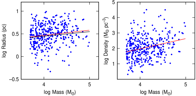
Figure 2: (Left) The radii and masses of clusters in two galaxies studied by Ryon et al. (2017) and the power-law fit to the small correlation between them. The black line is the fit from Larsen (2004). (Right) The density versus mass of clusters in Ryon et al., showing the power law fit between them. The fits are given by equations 24 and 25.

The values from Ryon et al. (2017) are plotted in Figure 2 with densities derived here, and the above fits are shown as red lines. There is a lot of scatter but a slight trend of radius with mass is evident. Larsen (2004) also determined a mass-size relation and got for 18 spiral galaxies $R=AM^{B}$ with $A=1.12\pm 0.35$ pc and $B=0.10\pm 0.03$. That fit is plotted on the left also, as a black line; it is almost identical to the fit using the data in Ryon et al. (2017).

Re-writing equation (25),

$$\left({{\rho_{\rm cluster}}\over{10^{4}\;M_{\odot}\;{\rm pc}^{-3}}}\right)=0.20\left({{M_{\rm cluster}}\over{10^{6}\;M_{\odot}}}\right)^{0.66},$$ (26)

which agrees with typical cluster densities in Portegies Zwart et al. (2010). This relation is assumed to be present at the time of cluster formation, rather than the result of a long evolution of cluster interactions (e.g., Gieles & Renaud, 2016).

Substituting this density dependence into equation (22) gives

$$\left({{M_{\rm cluster}}\over{10^{6}\;M_{\odot}}}\right)^{2.32}=28\left({{\Sigma_{\rm SFR}}\over{M_{\odot}\;{\rm pc}^{-2}\;{\rm Myr}^{-1}}}\right)^{2}$$ (27)

or

$$M_{\rm cluster}=4.2\times 10^{6}\;M_{\odot}\left({{\Sigma_{\rm SFR}}\over{M_{\odot}\;{\rm pc}^{-2}\;{\rm Myr}^{-1}}}\right)^{0.86}.$$ (28)

Similarly, equations (26) and (23) combine to give

$$M_{\rm cluster}=3.9\times 10^{6}\;M_{\odot}\left({{T_{\rm orb}}\over{100\;{\rm Myr}}}\right)^{1.3}\left({{\Sigma_{\rm SFR}}\over{M_{\odot}\;{\rm pc}^{-2}\;{\rm Myr}^{-1}}}\right)^{1.3}.$$ (29)

Johnson et al. (2017) suggest on the basis of 4 galaxies that the cut-off mass for the Schechter function is given by $\log(M_{\rm c})=(6.82\pm 0.20)+(1.07\pm 0.10)\log(\Sigma_{\rm SFR})$ in the usual units. For the Antennae galaxy in their data, where $\log(\Sigma_{\rm SFR})=-0.5$, they get $\log(M_{\rm c})=6.29$ and we get 6.19 from equation (28). For M83 and M51, where $\log(\Sigma_{\rm SFR})\sim-1.5$, they get 5.22 and we get 5.33. For M31, where $\log(\Sigma_{\rm SFR})\sim-2.7$, they get 3.93 and we get 4.30. These values are in reasonable agreement considering the approximations used for the assumed values of quantities in the pressure and star formation equations here. A direct comparison is in figure 3. The agreement could be made a little better by fine-tuning some of the assumed parameters, which are only rough estimates in this paper. Also shown in Figure 3 is equation (29) for $T_{\rm orb}=100$ Myr. This equation is not as good a fit, but it does not account for a possible variation in $T_{\rm orb}$ with $\Sigma_{\rm SFR}$.

4 The Size-of-Sample Mass compared to the Pressure-Limited Mass

For a given size and duration of a star-forming region, sections 2 and 3.2 suggest there is a relationship between the maximum expected mass of a cluster from the size-of-sample (SOS) effect (eq. 5) and the maximum expected mass from the interstellar pressure (eq. 28). If the SOS mass is less than the pressure mass, then the pressure limit is not likely to be observed because cluster masses will not be sampled far enough into the tail of the mass function to reach the pressure mass. A similar point was made by Gieles et al. (2006b). The pressure limit may be related to the cut-off mass, $M_{\rm c}$, in the Schechter function, or some other function with a cut-off, in which case the observation of a turn-over in this function depends on the relative values of these two masses.

In the present section, we identify the cluster mass derived from the cloud-core pressure and star formation surface density, as given in Section 3, with the cut-off mass in the cluster mass distribution function. It is convenient to write equations (5) and (28) in normalized form:

$$M_{\rm SOS,6}=2S\Delta t_{8}$$ (30)

$$M_{\rm c,6}=4.2\Sigma_{\rm SFR}^{0.86}$$ (31)

where mass with subscript 6 means in units of $10^{6}\;M_{\odot}$, $S$ is the star formation rate in $M_{\odot}$ yr^-1, $\Delta t_{8}$ is the duration of star formation in a typical large-scale region in units of $10^{8}$ yr, and $\Sigma_{\rm SFR}$ is in units of $M_{\odot}$ kpc^-2 yr^-1 (which is the same as $M_{\odot}$ pc^-2 Myr^-1).

The cutoff mass is observable in the cluster mass function if

$${{M_{\rm SOS,6}}\over{M_{\rm c,6}}}>1,$$ (32)

which is

$$S^{0.14}A^{0.86}\Delta t_{8}>2.1,\;\;{\rm or}\;\;\Sigma_{\rm SFR}^{0.14}A\Delta t_{8}>2.1$$ (33)

where we have written $\Sigma_{\rm SFR}=S/A$ for region area $A$ in kpc². This result hardly depends on the star formation rates $S$ or $\Sigma_{\rm SFR}$ but depends mostly on the size and duration of the star formation event, both of which have to be large, i.e. galaxy-scale, to see the cut-off mass. Even then, the maximum mass expected stochastically for a region, $M_{\rm SOS}$, is close to the maximum mass expected from the region pressure, i.e., the cut-off mass, which implies that the Schechter function form with the cut-off fully sampled should not be seen clearly in normal galaxies. In fact, it is barely perceptible in the differential mass functions shown by Adamo et al. (2017) and Messa et al. (2017). The cut-off will be seen best in large galaxies (high $A$) with long durations of star formation ($\Delta t$) in each region.

For a given $\Delta t$, equations (30) and (31) suggest more simply that the cut-off mass is best seen in galaxies with high star formation rates and low rate densities, which means large, fairly inactive, galaxies. Large, low-surface brightness galaxies or large galaxies with fairly low $\Sigma_{\rm SFR}$ are good examples where the cut-off mass in the Schechter function should be observable according to these conditions. This is because the pressure is low in these galaxies, so the maximum cluster mass should be low, but there could be a lot of clusters in the large disk, sampling far out in the mass function tail.

5 Comparison to Observations at high redshift

Star-forming regions in high-redshift galaxies often exceed the two limits discussed above, suggesting they commonly make $10^{6}\;M_{\odot}$ YMCs. This is consistent with the discussion in the Introduction which offered many examples where GC formation was pervasive in the early universe.

Guo et al. (2018) measured star formation rates in over 3000 clumps in $\sim 1000$ galaxies at redshifts from 0.5 to 3. Figure 4 shows the distribution functions of these rates sorted by redshift. The red vertical line in each panel is the $1\;M_{\odot}$ yr^-1 threshold for YMC formation from Section 2. Background subtraction by the fiducial method was used. The clump SFRs increase with redshift because of the selection of brighter and more massive galaxies at greater distances. The decrease in SFR at low SFR is probably a selection effect too, since fainter regions are more difficult to see. At the high-mass end, the distribution functions fall off approximately as power laws. The three slopes are $-0.85\pm 0.06$ for $z=0.5-1$, $-0.85\pm 0.06$ for $z=1-2$ and $-0.68\pm 0.10$ for $z=2-3$. These are close to the slope of $\sim-1$ (on a log-log plot) of the mass functions of clusters and OB associations locally (Portegies Zwart et al., 2010), although Figure 4 has SFR instead of mass. Clump mass functions with this slope were obtained by Dessauges-Zavadsky et al. (2018) using a different sample of high redshift clumps. For a $-2$ slope, there is an equal amount of star formation in each equal interval of the log of the SFR. Since the $1\;M_{\odot}$ yr^-1 limit about equally divides the log SFR scale, approximately half of the star formation in these clumps is in regions that can produce a $10^{6}\;M_{\odot}$ cluster. In fact, the fraction of the observed clump star formation with a local clump rate greater than $1\;M_{\odot}$ yr^-1 is 0.46, 0.61 and 0.72 for the three redshift bins in the figure, respectively.

The surface density of star formation in the Guo et al. (2018) clumps cannot be measured because their resolution at $z\sim 1$ is only 1.5 kpc diameter. However, dividing the star formation rates by the area at 1.5 kpc diameter, which is 1.8 kpc², gives a rate density that is also comparable to the above limits, namely $\sim 0.5\;M_{\odot}$ pc^-2 Myr^-1. This is a lower limit to the rate density because the regions are probably smaller than the resolution.

Star forming clumps at high redshift have also been measured in lensed systems. Cava et al. (2018) resolved clumps down to 30 pc and $10^{7}\;M_{\odot}$ in the “snake”. They found that 55 clumps represent about half of the total star formation rate of $30\;M_{\odot}$ yr^-1, so the average rate among them is $\sim 0.24\;M_{\odot}$ yr^-1. The most massive of the blue clumps contains $\sim 10^{8.5}\;M_{\odot}$ of stars in a radius of $\sim 300$ pc. If most of these stars formed in $\sim 100$ Myr, then the two rates are $3\;M_{\odot}$ yr^-1 and $\sim 10\;M_{\odot}$ pc^-2 Myr^-1, both over the threshold for forming a $10^{6}\;M_{\odot}$ YMC.

High spatial resolution is also possible in local galaxies that are analogous to high redshift galaxies in their clump properties. Overzier et al. (2009) studied 37 clumps in 30 galaxies with $0.1^{\prime\prime}$ resolution at redshifts between 0.1 and 0.3. The average clump radius was 200-400 pc and the average star formation rate among all the clumps was $0.95\pm 0.46\;M_{\odot}$ yr^-1. These quantities give an average rate density of $\sim 3\;M_{\odot}$ pc^-2 Myr^-1. Both values suggest the likely formation of $10^{6}\;M_{\odot}$ clusters according to the present model.

6 Uncertainties

This paper considers a cluster mass function that has a characteristic mass below which the slope is the canonical $-2$ and above which the number of clusters drops more rapidly. There have been several explanations for this “cut-off” or “maximum” mass, including fixed fractions of the Jeans mass (Kruijssen, 2014) or the rotationally stabilized mass (Escala & Larson, 2008) in a galaxy disk. Some discussion of early models is in Gieles et al. (2006b). Cosmological simulations by Li et al. (2017) get a power-law cluster mass function with an upper cut-off too; in their models, the upper cut-off mass increases with total star formation rate, but they do not consider the dependence of this cut-off on the star formation rate density, as in the present paper.

Here we propose that the maximum cluster mass is primarily related to the pressure in the core of a cluster-forming cloud according to the virial theorem with a density equal to some fixed factor times the density of the cluster. This core pressure is then assumed to be $\sim 10^{4}$ times the interstellar pressure – considering that self-gravitating clouds typically have an internal density structure that varies approximately with the second power of the inverse of radius, and because cloud core radii are about 1% the size of the disk scale height. The interstellar pressure is then related to the gas surface density by the usual equilibrium equation, and the gas surface density is related to the star formation rate surface density by the Kennicutt-Schmidt relation. The result is a cluster cut-off mass for local galaxies that scales with the 0.86 power of the star formation rate surface density, and with a normalization that agrees with observations. Feedback is assumed to play little role in this maximum cluster mass because the mass is typically so large that the stellar IMF is fully sampled and the luminosity-to-mass ratio of the stellar mixture has no feature or sudden increase that might lead to excess disruption of more massive clusters.

Most of the assumptions involved seem to have only a small influence on the results. A minor role is played by the assumption that the magnetic and cosmic ray pressures in a galaxy disk nearly balance the stellar and dark matter contributions to disk self-gravity ($\xi/\zeta\sim 1$); this ratio of parameters is not likely to deviate much from unity, and it agrees with local observations. Secondly, the ratio of the stellar mass to the virial mass in a cluster-forming core, or stellar density to virial density, was taken to be represented by the composite efficiency fraction $\epsilon\sim 0.5$. For the so-called conveyer-belt model of cluster formation (Sect. 3.1), this dimensionless parameter could be larger than 1, but it is not likely to be much smaller than 0.5 to get a bound cluster. Cosmological simulations (e.g. Kimm et al., 2016; Ricotti et al., 2016; Kim et al., 2018) get high cluster-formation efficiencies from direct collapse, also supporting a value of $\epsilon$ within a factor of 2 of $\sim 0.5$. This parameter enters $M_{\rm c}$ as $\epsilon^{0.43}$ from equations (21) and (27), so the influence on the result is small. The efficiency per unit free fall time and disk scale height for star formation on a galactic scale in the Kennicutt-Schmidt relation were assumed to be $\epsilon_{\rm ff}\sim 0.01$ and $H\sim 100$ pc, but these are important only if the KS law is derived from first principles; if the empirical law is used, which is reproduced by these values, then this assumption is not needed. Thus we consider this to be a weak influence on the result also. Another component is the observed relation between the cluster density and mass, where we used observations from Ryon et al. (2017), reduced to equations (25) and (26), and which are also in agreement with a similar measurement by Larsen (2004). Because this is tied to observations, we consider the uncertainty to be small, but the scatter in the relation is large and the physical origin of it is unknown.

A more important role is played by the compaction factor $C\sim 10^{4}$, which, as mentioned above, is the ratio of the pressure in a cluster-forming cloud core to the ambient pressure in the interstellar medium. This was estimated from observations in Section 3.2, so it is not totally unknown, but it could vary with environment in unknown ways. According to equations (21) and (27), it enters into $M_{\rm c}$ as $C^{0.64}$. The value of $10^{4}$ for a cloud density profile that varies as the inverse square of radius is equivalent to a cluster-forming core with 1% of the total cloud mass, giving our pressure-based theory some connection to the mass-based theories in Kruijssen (2014) and Escala & Larson (2008).

Ultimately, the relation between $M_{\rm c}$ and $\Sigma_{\rm SFR}$ will be measured for many galaxies, and there will also be better measurements of $C$ and the other parameters suggested here to be important. Then the basic model where maximum cluster mass depends primarily on interstellar pressure can be checked more thoroughly.

7 Conclusions

The history of star formation in the universe and the build-up of stellar mass with time both suggest that before a redshift of $\sim 2$, which is the time of peak universal star formation, most regions that formed stars also formed GCs and their associated unbound stars. Today, only the most extreme regions of star formation form GCs. The transition that must have occurred in cluster-forming gas is proposed to be the result of a decrease in both the total star formation rate and the rate per unit area for each independent region, with threshold values of $\sim 1\;M_{\odot}$ yr^-1 and $\sim 1\;M_{\odot}$ pc^-2 Myr^-1, respectively, more commonly exceeded in the early universe.

The maximum mass of a cluster with a characteristic density was linked to the star formation surface density using the virial equation for cloud core pressure, a compaction factor that links cloud cores to average interstellar pressures, an equilibrium equation that associates interstellar pressure with gas surface density on large-scales, and the Kennicutt-Schmidt relation between gas surface density and star formation rate surface density. There are many links in this chain, but each has an observational basis, and the resultant maximum mass agrees with the observed cluster cut-off mass for a wide range of star formation rate densities (Fig. 3).

The threshold star formation rate and rate density derived here also agree with observed values in high redshift clumps (Fig. 4), confirming that these common regions could be the formation sites for most of today’s GCs, with lower-mass galaxies forming the more metal-poor GCs. The rate density for GC formation corresponds to a gas surface density of several hundred to a thousand $M_{\odot}$ pc^-2, which is much larger than in today’s galaxies but was common at high redshift.

Acknowledgement: I am grateful to the referee for useful comments.

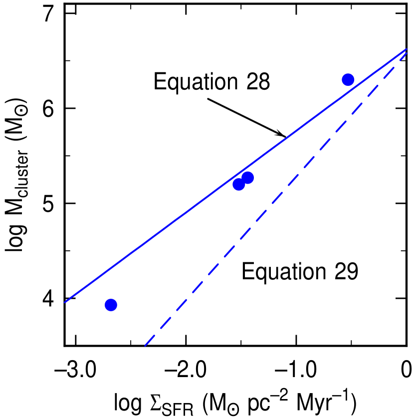
Figure 3: The maximum cluster mass as determined from the ISM pressure, cloud virial equilibrium, and observed cluster density, with a compaction factor of $C=10^{4}$ to convert ISM pressure to cloud core pressure, plotted versus the star formation rate density, which also correlates with the ISM pressure through the average gas surface density. The plotted points are from Johnson et al. (2017) for the cut-off mass in four galaxies: M31 at low $\Sigma_{\rm SFR}$, M83 and M51 at intermediate values and the Antennae at the high value. We identify the maximum cluster mass as determined from ISM pressure with the cut-off mass in the cluster mass function. The solid line uses the Kennicutt-Schmidt relation with a $\Sigma_{\rm gas}^{1.5}$ dependence tied to observations at low redshift but also approximately applicable at intermediate redshifts, and the dashed line uses the form of the Kennicutt-Schmidt relation where the star formation rate density is taken to scale with the inverse of the orbit time. The latter fit is not as good, but the orbit time is probably not constant with $\Sigma_{\rm SFR}$ as assumed here; variation of $T_{\rm orb}$ with the inverse square root of the gas surface density would make these two lines parallel.

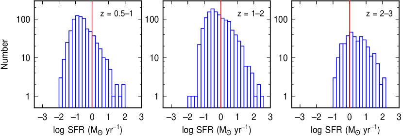
Figure 4: Distribution function for star formation rates in the giant clumps of galaxies studied by Guo et al. (2018), divided into three redshift bins. The suggested lower limit for the formation of a $10^{6}\;M_{\odot}$ cluster by the size-of-sample effect is indicated by the red vertical line. Approximately half of the star formation in the measured clumps occurs in active-enough clumps to sample a $10^{6}\;M_{\odot}$ cluster. Because these regions are also typically smaller than a kiloparsec, the surface density of star formation also exceeds the limit for a $10^{6}\;M_{\odot}$ cluster to the right of the red line.

References

- Adamo et al. (2011) Adamo, A., Östlin, G., Zackrisson, E., Papaderos, P., Bergvall, N., Rich, R. M., & Micheva, G. 2011, MNRAS, 415, 2388
- Adamo et al. (2015) Adamo, A., Kruijssen, J. M. D., Bastian, N., Silva-Villa, E., & Ryon, J. 2015, MNRAS, 452, 246
- Adamo et al. (2017) Adamo A., Ryon, J.E., Messa, M., et al., 2017, ApJ, 841, 131
- Bastian et al. (2012) Bastian, N., Adamo, A., Gieles, M., Silva-Villa, E., Lamers, H.J.G.L. M., Larsen, S. S., Smith, L. J., Konstantopoulos, I. S., Zackrisson, E. 2012, MNRAS, 419, 2606
- Bastian et al. (2014) Bastian, N., Hollyhead, K., & Cabrera-Ziri, I. 2014, MNRAS, 445, 378
- Bastian & Lardo (2018) Bastian, N., & Lardo, C. 2018, ARA&A, 56, 83
- Bell et al. (2008) Bell, E.F., Zucker, D.B., Belokurov, V. et al., 2008, ApJ, 680, 295
- Bigiel et al. (2008) Bigiel, F., Leroy, A., Walter, F., Brinks, E., de Blok, W. J. G., Madore, B., & Thornley, M. D. 2008, AJ, 136, 2846
- Billett et al. (2002) Billett, O.H., Hunter, D.A., & Elmegreen, B.G. 2002, AJ, 123, 1454
- Boulares & Cox (1990) Boulares, A., & Cox, D.P. 1990, ApJ, 365, 544
- Boylan-Kolchin (2017) Boylan-Kolchin, M. 2017, MNRAS, 472, 3120
- Boylan-Kolchin (2018) Boylan-Kolchin, M. 2018, MNRAS, 479, 332
- Bressert et al. (2010) Bressert, E., Bastian, N., Gutermuth, R., et al. 2010, MNRAS, 409, L54
- Brodie & Strader (2006) Brodie, J. P., & Strader, J. 2006, ARA&A, 44, 193
- Calzetti et al. (2015) Calzetti, D., Johnson, K. E., Adamo, A. et al. 2015, ApJ, 811, 75
- Carraro et al. (2007) Carraro, G., Zinn, R., & Moni Bidin, C. 2007, A&A, 466, 181
- Casetti-Dinescu, et al. (2009) Casetti-Dinescu, D.I., Girard, T.M., Majewski, S.R., et al. 2009, ApJL, 701, L29
- Cava et al. (2018) Cava, A., Schaerer, D., Richard, J., Pérez-González, P.G., Dessauges-Zavadsky, M., Mayer, L., & Tamburello, V. 2018, Nature Astron, 2, 76
- Chandar et al. (2017) Chandar, R., Fall, S. M., Whitmore, B.C., Mulia, A.J. 2017, ApJ, 849, 128
- Cohen et al. (2018) Cohen, D.P., Turner, J.L., Consiglio, S.M., Martin, E.C., Beck, S.C. 2018, ApJ, 860, 47
- Corbelli et al. (2018) Corbelli, E., Elmegreen, B.G., Braine, J., & Thilker, D. 2018, A&A, in press, arXiv 1807.00166
- Da Costa & Armandroff (1995) Da Costa, G. S., Armandroff, T. E. 1995, AJ, 109, 2533
- Deason et al. (2011) Deason, A. J., Belokurov, V., & Evans, N. W. 2011, MNRAS, 416, 2903
- De Marchi et al. (1997) De Marchi, G., Clampin, M., Greggio, L., Leitherer, C., Nota, A., Tosi, M. 1997, ApJL, 479, L27
- Dessauges-Zavadsky et al. (2018) Dessauges-Zavadsky, M., Adamo, A. 2018, MNRAS, 479, L118
- Druard et al. (2014) Druard, C., Braine, J., Schuster, K.F., et al. 2014, A&A, 567, A118
- Elmegreen (1989) Elmegreen, B.G. 1989, ApJ, 388, 178
- Elmegreen (2018) Elmegreen, B.G. 2018, ApJ, 854, 16
- Elmegreen & Elmegreen (1987) Elmegreen, B.G., & Elmegreen, D.M. 1987, ApJ, 320, 182
- Elmegreen & Efremov (1997) Elmegreen, B.G. & Efremov, Y.N. 1997, ApJ, 480, 235
- Elmegreen et al. (2012) Elmegreen, B.G, Malhotra, S., & Rhoads, J. 2012, ApJ, 757, 9
- Elmegreen (2015) Elmegreen, B.G. 2015, ApJ, 814, L30 (Paper I).
- Elmegreen et al. (2016) Elmegreen, D.M., Elmegreen, B.G., Sánchez Almeida, J., Muñoz-Tuñón, C., Mendez-Abreu, J., Gallagher, J.S., Rafelski, M., Filho, M., Ceverino, D., 2016, ApJ, 825, 145
- Elmegreen & Elmegreen (2017a) Elmegreen, D.M. & Elmegreen, B.G. 2017, ApJL, 851, L44
- Elmegreen et al. (2017) Elmegreen, B.G., Elmegreen, D.M., Tompkins, B., & Jenks, L.G. 2017, ApJ, 847, 14
- Elmegreen et al. (2018) Elmegreen, B.G., Herrera, C., Rubio, M., Elmegreen, D.M., Sánchez Almeida, J., Muñoz-Tuñón, C., & Olmo-García, A. 2018, ApJ, 859, L22
- Escala & Larson (2008) Escala, A., & Larson, R.B. 2008, ApJ, 685, L31
- Finkelstein et al. (2015) Finkelstein, K.D., Finkelstein, S.L., & Tilvi, V. et al. 2015, ApJ, 813, 78
- Fleck (1996) Fleck, R. C., Jr. 1996, ApJ, 458, 739
- Forbes & Bridges (2010) Forbes, D.A., & Bridges, T. 2010, MNRAS, 404, 1203
- Förster-Schreiber et al. (2009) Förster Schreiber, N.M., Genzel, R., Bouché, N. et al. 2009, ApJ, 706, 1364
- Freeman (1993) Freeman, K.C. 1993, in The Globular Cluster-Galaxy Connection, ASP Conference Series 48, eds. G.H. Smith and J.P. Brodie, 608
- Galván-Madrid et al. (2017) Galván-Madrid, R., Liu, H.B., Ginsburg, A., & Pineda, J.E. 2017, RevMexAA, Serie de Conferencias, 49, 104
- Gao et al. (2007) Gao, S., Jiang, B.-W., & Zhao, Y.-H. 2007, ChJAA, 7, 111
- Gieles et al. (2006a) Gieles, M., Larsen, S. S., Scheepmaker, R.A., Bastian, N., Haas, M.R., Lamers, H. J. G. L. M. 2006, A&A, 446, L9
- Gieles et al. (2006b) Gieles M., Larsen S. S., Bastian N., Stein I. T., 2006, A&A, 450, 129
- Gieles & Renaud (2016) Gieles, M. & Renaud, F. 2016, MNRAS, 463, L103
- Gilbert & Graham (2002) Gilbert, A. M., & Graham, J. R. 2002, in IAU Symp. 207, Extragalactic Star Clusters, ed. D. Geisler, E. K. Grebel, & D. Minniti (San Francisco, CA: ASP), 471
- Ginsburg et al. (2016) Ginsburg, A., Goss, W. M., & Goddi, C. 2016, A&A, 595A, 27
- Girichidis et al. (2012) Girichidis, P., Federrath, C., Banerjee, R., Klessen, R.S. 2012, MNRAS, 420, 613
- Grabelsky et al. (1987) Grabelsky, D. A., Cohen, R. S., Bronfman, L., Thaddeus, P., & May, J. 1987, ApJ, 315, 122
- Greggio et al. (1998) Greggio, L., Tosi, M., Clampin, M., De Marchi, G., Leitherer, C., Nota, A., & Sirianni, M. 1998, ApJ, 504, 725
- Guo et al. (2018) Guo, Y., Rafelski, M., Bell, E.F. et al. 2018, Apj, 853, 108
- Harris (1991) Harris, W.E. 1991, ARA&A, 29, 543
- Harris (2001) Harris, W.E. 2001, in Star Clusters, Saas-Fee Advanced Courses, Volume 28. ISBN 978-3-540-67646-1. Springer-Verlag Berlin Heidelberg, p. 223
- Heyer & Dame (2015) Heyer, M., & Dame, T.M. 2015, ARA&A, 53, 583
- Ibata et al. (1994) Ibata R. A., Gilmore G., Irwin M. J., 1994, Nature, 370, 194
- Inoue et al. (2016) Inoue, S., Dekel, A., Mandelker, N., Ceverino, D., Bournaud, F., & Primack, J. 2016, MNRAS, 456, 2052
- Jordán et al. (2007) Jordán, A., McLaughlin, D.E., Côté, P., et al. 2007, ApJS, 171, 101
- Johnson et al. (2012) Johnson, M., Hunter, D.A., Oh, S.-H., Zhang, H.-X., Elmegreen, B., Brinks, E., Tollerud, E., Herrmann, K. 2012, AJ, 144, 152
- Johnson et al. (2017) Johnson, T.L., Rigby, J.R., Sharon, K., et al. 2017, ApJL, 843, L21
- Johnson et al. (2012) Johnson, M., Hunter, D.A., Oh, S.-H., Zhang, H.-X., Elmegreen, B., Brinks, E., Tollerud, E., & Herrmann, K. 2012, AJ, 144, 152
- Kennicutt & Evans (2012) Kennicutt R. C., & Evans N. J., 2012, ARA&A, 50, 531
- Kim et al. (2018) Kim, J.-h., Ma, X., Grudić, M.Y., Hopkins, P.F., Hayward, C.C., Wetzel, A., Faucher-Giguère, C.-A., Kereš, D,. Garrison-Kimmel, S., & Murray, N. 2018, MNRAS, 474, 4232
- Kimm et al. (2016) Kimm, T., Cen, R., Rosdahl, J., Yi, S.K. 2016, ApJ, 823, 52
- Kravtsov & Gnedin (2005) Kravtsov, A.V. & Gnedin, O.Y. 2005, ApJ, 623, 650
- Krumholz et al. (2012) Krumholz, M. R., Dekel, A., & McKee, C. F. 2012, ApJ, 745, 69
- Kruijssen (2012) Kruijssen, J. M. D. 2012, MNRAS, 426, 3008
- Kruijssen (2014) Kruijssen, J.M.D. 2014, Classical and Quantum Gravity, Vol. 31, Issue 24, article id. 244006
- Kruijssen (2015) Kruijssen J. M. D., 2015, MNRAS, 454, 1658
- Kruijssen & Cooper (2012) Kruijssen, J.M.D., & Cooper, A.P. 2012, MNRAS, 420, 340
- Kruijssen et al. (2018) Kruijssen, J. M. D., Pfeffer, Joel L., Reina-Campos, M., Crain, R.A., & Bastian, N. 2018, MNRAS, tmp1537
- Krumholz & Tan (2007) Krumholz, M.R. & Tan, J.C. 2007, ApJ, 654, 304
- Krumholz et al. (2018) Krumholz, M.R., McKee, C.F., & Bland-Hawthorn, J. 2018, ARA&A, in press
- Lada et al. (1988) Lada, C.J., Margulis, M., Sofue, Y., Nakai, N., Handa, T. 1988, ApJ, 328, 143
- Lada et al. (1997) Lada, E.A., Evans, N.J., II, & Falgarone, E. 1997, ApJ 488, 286
- Lada & Lada (2003) Lada, C.J. & Lada, E.A. 2003, ARA&A, 41, 57
- Larsen (2002) Larsen, S.S. 2002, AJ, 124, 1393
- Larsen (2004) Larsen, S.S. 2004, A&A, 416, 537
- Larsen (2009) Larsen, S.S. 2009, A&A, 494, 539
- Larsen & Richtler (2000) Larsen, S. S., & Richtler, T. 2000, A&A, 354, 836
- Larsen et al. (2012) Larsen, S.S., Strader, J., & Brodie, J.P. 2012, A&A, 544L, 14
- Larsen et al. (2014) Larsen, S.S., Brodie, J.P., Forbes, D.A., & Strader, J. 2014 A&A, 565A, 98
- Larsen et al. (2011) Larsen, S. S., de Mink, S. E., Eldridge, J. J., Langer, N., Bastian, N., Seth, A., Smith, L. J., Brodie, J., Efremov, Yu. N. 2011, A&A, 532A, 147
- Larsen et al. (2018) Larsen, S. S., Brodie, J. P., Wasserman, A. & Strader, J. 2018, A&A, 613A, 56
- Law & Majewski (2010) Law, D.R. & Majewski, S.R. 2010, ApJ, 718, 1128
- Leaman et al. (2012) Leaman, R., Venn, K.A., Brooks, A.M., et al. 2012, ApJ, 750, 33
- Lelli et al. (2014) Lelli, F., Verheijen, M., & Fraternali, F. 2014, MNRAS, 445, 1694
- Li et al. (2017) Li, H., Gnedin, O.Y., Gnedin, N.Y., Meng, X., Semenov, V.A., Kravtsov, A.V., 2017, ApJ, 834, 69
- Lin et al. (2017) Lin, Y., Liu, H.B., Dale, J.E. et al. 2017, ApJ, 840, 22
- Longmore et al. (2014) Longmore, S. N., Kruijssen, J. M. D., Bastian, N., Bally, J., Rathborne, J., Testi, L., Stolte, A., Dale, J., Bressert, E., & Alves, J. 2014, Protostars and Planets VI, eds. H. Beuther, R. S. Klessen, C. P. Dullemond, & T. Henning, Tucson: University of Arizona Press, p.291
- López-Sánchez et al. (2012) López-Sánchez, Á. R., Koribalski, B. S., van Eymeren, J., Esteban, C., Kirby, E., Jerjen, H., & Lonsdale, N. 2012, MNRAS, 419, 1051
- Mackey & Gilmore (2004) Mackey A. D., & Gilmore G. F., 2004, MNRAS, 355, 504
- Mackey et al. (2010) Mackey, A. D., Huxor, A. P., Ferguson, A.M.N., Irwin, M.J., Tanvir, N. R., McConnachie, A. W., Ibata, R. A., Chapman, S. C., Lewis, G. F., 2010, ApJ, 717, L11
- Madau & Dickinson (2014) Madau, P. & Dickinson, M. 2014, ARA&A, 52, 415
- Mannucci et al. (2009) Mannucci F. et al., 2009, MNRAS, 398, 1915
- Martell et al. (2016) Martell, S.L., Shetrone, M.D., Lucatello, S., Schiavon, R.P., Mészáros, S., Allende Prieto, C., García-Hernández, D. A., Beers, T.C., & Nidever, D.L. 2016, ApJ, 825, 146
- Martell (2017) Martell, S.L. 2017, Proceedings IAU Symposium No. 134, eds. C. Chiappini, I. Minchev, E. Starkenburg, & M. Valentini, Cambridge: Cambridge University Press, in press
- Martin et al. (2004) Martin N. F., Ibata R. A., Bellazzini M., Irwin M. J., Lewis G.F., Dehnen W., 2004, MNRAS, 348, 12
- Matzner & Jumper (2015) Matzner, C.D. & Jumper, P.H. 2015, ApJ, 815, 68
- Matzner (2017) Matzner, C.D. 2017, in Proceedings of the Star Formation in Different Environments, ICISE, Quy Nhon, Vietnam, 2016, eds. D. Johnstone, T. Hoang, F. Nakamura, Q. Nguyen-Luong, and J. T. Tranh Van, arXiv171201457
- McKee & Ostriker (2007) McKee, C.F., & Ostriker, E.C. 2007, ARA&A, 45, 565
- McKee et al. (2015) McKee, C.F., Parravano, A., & Hollenbach, D.J. 2015, ApJ, 814, 13
- Messa et al. (2017) Messa, M., Adamo, A., Östlin, G., et al. 2017, MNRAS, 473, 996
- Messa et al. (2018) Messa, M., Adamo, A., Calzetti, D., et al. 2018, MNRAS, 477, 1683
- Miura et al. (2015) Miura, R.E., Espada, D., Sugai, H., Nakanishi, K., Hirota, A. 2015, PASJ, 67, L1
- Morrison (1993) Morrison, H.L. 1993, AJ, 106, 578
- Mueller et al. (2002) Mueller, K. E., Shirley, Y. L., Evans, N.J., II, & Jacobson, H. R. 2002, ApJS, 143, 469
- Murray & Chang (2015) Murray, N., & Chang, P. 2015, ApJ, 804, 44
- Myeong et al. (2018) Myeong, G. C., Evans, N. W., Belokurov, V., Sanders, J. L., Koposov, S. E. 2018, arXiv180500453
- Newberg et al. (2009) Newberg, H.J., Yanny, B., & Willett, B.A. 2009, ApJ, 700, L61
- Overzier et al. (2009) Overzier, R.A., Heckman, T.M., Tremonti, C. et al. 2009, ApJ, 706, 203
- Palma et al. (2002) Palma C., Majewski S. R., & Johnston K.V., 2002, ApJ, 564, 736
- Portegies Zwart & McMillan (2000) Portegies Zwart, S. F., & McMillan, S. L. W. 2000, ApJ, 528, L17
- Portegies Zwart et al. (2010) Portegies Zwart, S.F., McMillan, S.L.W. & Gieles, M. 2010, ARA&A 48, 431
- Randriamanakoto et al. (2013) Randriamanakoto, Z., Escala, A., Väisänen, P., Kankare, E., Kotilainen, J., Mattila, S., & Ryder, S. 2013, ApJL, 775, L38
- Rice et al. (2016) Rice, T.S., Goodman, A.A., Bergin, E.A., Beaumont, C., Dame, T. M. 2916, ApJ, 822, 52
- Ricotti et al. (2016) Ricotti, M., Parry, O.H., & Gnedin, N.Y. 2016, ApJ, 831, 204
- Rossi & Hurley (2015) Rossi, L. J. & Hurley, J. R. 2015, MNRAS, 446, 3389
- Ryon et al. (2017) Ryon, J.E., Gallagher, J.S., Smith, L.J. et al. 2017 ApJ, 841, 92
- Sabbi et al. (2018) Sabbi, E., Calzetti, D., Ubeda, L. et al. 2018, ApJS, 235, 23
- Searle & Zinn (1978) Searle L., & Zinn R. 1978, ApJ, 225, 357
- Shapiro et al. (2010) Shapiro, K.L., Genzel, R., & Förster Schreiber, N.M. 2010, MNRAS, 403, L36
- Shu (1977) Shu, F.H. 1977, ApJ, 214, 488
- Silich & Tenorio-Tagle (2018) Silich, S., & Tenorio-Tagle, G. 2018, MNRAS, 478, 5112
- Smith et al. (2009) Smith, M. C., Evans, N. W., Belokurov, V., et al. 2009, MNRAS, 399, 1223
- Sollima & Baumgardt (2017) Sollima, A. & Baumgardt, H. 2017, MNRAS, 471, 3668
- Stil & Israel (1998) Stil, J. M., & Israel, F. P. 1998, A&A, 337, 64
- Strader et al. (2011) Strader, J., Romanowsky, A.J., Brodie, J.P., et al. 2011, ApJS, 197, 33
- Tacconi et al. (2018) Tacconi, L. J., Genzel, R., Saintonge, A., et al. 2018, ApJ, 853, 179
- Tan et al. (2014) Tan, J. C., Beltrán, M. T., Caselli, P., Fontani, F., Fuente, A., Krumholz, M. R., McKee, C. F., Stolte, A. 2014 in Protostars and Planets VI, Henrik Beuther, Ralf S. Klessen, Cornelis P. Dullemond, and Thomas Henning (eds.), University of Arizona Press, Tucson, 914 pp., p.149-172
- Tonini (2013) Tonini, C. 2013, ApJ, 762, 39
- Tsang & Milosavljević (2018) Tsang, B.T.-H., & Milosavljević, M. 2018, MNRAS, 478, 4142
- Turner et al. (2015) Turner, J. L., Beck, S. C., Benford, D. J., Consiglio, S. M., Ho, P.T.P., Kovács, A., Meier, D. S., Zhao, J.-H. 2015, Nature, 519, 331
- Vacca et al. (1996) Vacca, W.D., Garmany, C.D., & Shull, J.M. 1996, ApJ, 460, 914
- van den Bergh (2007) van den Bergh, S. 2007, AJ, 134, 344
- Vanzella et al. (2017) Vanzella, E., Calura, F., Meneghetti, M., et al. 2017, MNRAS, 467, 4304
- Vesperini (1998) Vesperini E., 1998, MNRAS, 299, 1019
- Yozin & Bekki (2012) Yozin, C., & Bekki, K. 2012, ApJL, 756, L18
- Walker et al. (2016) Walker, D. L., Longmore, S. N., Bastian, N., Kruijssen, J. M. D., Rathborne, J. M., Galván-Madrid, R., Liu, H. B. 2016, MNRAS, 457, 4536
- Ward & Kruijssen (2018) Ward, J.L., & Kruijssen, J.M.D. 2018, MNRAS, 475, 5659
- Whitmore et al. (2010) Whitmore, B.C., Chandar, R., Schweizer, F. et al. 2010, AJ, 140, 75
- Whitmore et al. (2014) Whitmore, B.C., Chandar, R., Bowers, A.S., Larsen, S., Lindsay, K., Ansari, A., Evans, J. 2014, AJ, 147, 78
- Zaritsky et al. (2016) Zaritsky, D., McCabe, K., Aravena, M. et al. 2016, ApJ, 818, 99
- Zheng et al. (2017) Zheng, Z.-Y., Wang, J., Rhoads, J., et al. 2017, ApJ, 842, L22
- Zinnecker et al. (1988) Zinnecker, H., Keable, C. J., Dunlop, J.S., Cannon, R.D., Griffiths, W. K. 1988, IAUS, 126, 603