Periodic Event-triggered Control for Incrementally Quadratic Nonlinear Systems

Abstract

Periodic event-triggered control (PETC) evaluates the triggering rule periodically and is well-suited for implementation on digital platforms. This paper investigates PETC design for nonlinear systems affected by external disturbances under the impulsive system formulation. Sufficient conditions are provided to ensure the input-to-state stability of the resulting closed-loop system for the state feedback and the observer-based output feedback configurations separately. For each configuration, the sampling period and the triggering functions are provided explicitly. Sufficient conditions in the form of linear matrix inequalities are provided for the PETC design of incrementally quadratic nonlinear systems. Two examples are given to illustrate the effectiveness of the proposed method.

1 Introduction

Digital control systems are traditionally executed in a time-triggered fashion where the sensors and actuators are accessed periodically. In contrast, event-triggered control (ETC) executes the communication and actuation only when certain triggering rules are satisfied; this can be seen as adding feedback to the communication and actuation processes (see a recent survey paper [1] and references therein). The ETC paradigm is designed to avoid unnecessary waste of communication/computation resources by reducing the number of communication/actuation executions, while still guaranteeing a desirable closed-loop performance [2, 3, 4, 5, 6, 7, 8, 9]; this shows potential in applications of systems with limited communication bandwidth such as networked control systems.

Since the triggering condition of ETC has to be monitored continuously, it is difficult to implement ETC in digital platforms directly. By evaluating the triggering conditions and deciding whether to update the communication/actuation at each periodic sampling time, periodic event-triggered control (PETC) inherits advantages of ETC and can be implemented on standard digital platforms [10, 11, 12]. Furthermore, Zeno phenomenon is avoided since the sampling period is a lower bound for the minimum inter-execution time. Although ETC for discrete-time models can be considered as PETC (e.g., see [11, 13]), the inter-sample behavior of the original continuous-time systems are not captured in the discrete-time analysis. PETC design for (continuous-time) linear systems was investigated in [10, 14]. However, PETC design for nonlinear systems is difficult because of an intrinsic difficulty: the discrete-time dynamics of a nonlinear system can not be exactly known from its continuous-time dynamics [15, 16, 17, 18, 19]. There are few existing papers on PETC design for nonlinear systems: [17] studied state feedback PETC design for undisturbed nonlinear systems using the hybrid system approach and proved globally asymptotically stability of the closed-loop system; [20] studied output feedback PETC design for disturbed nonlinear systems; [21] extended the results of [17, 20] to the decentralized setting; [16] investigated state feedback PETC design for nonlinear systems by redesigning the event function of an existing continuous ETC system using overapproximation techniques, such that control performance guarantees for the continuous ETC system are preserved; [15] studied output feedback PETC design for Lipschitz systems using impulsive observers and proved practical stabilization of the resulting system. In spite of these interesting results, many PETC design problems for nonlinear systems are largely open and deserve to be further explored.

This paper investigates input-to-state stabilization of disturbed nonlinear systems under PETC mechanisms. An impulsive system approach is used for modeling and analyzing the overall system. Under the assumption that there exists a sum-type ISS-Lyapunov function for the continuous dynamics, the sampling period and triggering functions are designed such that the overall system is ISS using the same ISS-Lyapunov function. The contributions of the paper are at least two-fold: (i) This work provides sufficient conditions for the input-to-state stabilization of nonlinear systems affected by disturbances using state feedback or observer-based output feedback PETC design. (ii) This work presents sufficient conditions in the form of linear matrix inequalities (LMIs) for the PETC design of incrementally quadratic nonlinear systems, which subsumes many class of nonlinear systems including the Lipschitz nonlinear systems. Degeneration of the general results to linear control systems is also discussed. Compared with [21, 17, 20], this work does not rely on the small-gain techniques for hybrid systems, and provides LMI conditions for more general class of systems; compared with [16, 15], the work considers general nonlinear dynamics with external disturbances.

Notation. Denote the set of real, non-negative real and non-negative integer numbers by $\mathbb{R}$, $\mathbb{R}_{\geq 0}$ and $\mathbb{Z}_{\geq 0}$, respectively. Denote the 2-norm by $\|\cdot\|$. Given a non-empty and closed set $\mathcal{A}$, the point-to-set distance from $x$ to $\mathcal{A}$ is denoted by $\|x\|_{\mathcal{A}}=\inf_{y\in\mathcal{A}}\|y-x\|$. Denote the identity matrix of size $n\times n$ by $I_{n}$. Denote the zero matrix of size $n_{1}\times n_{2}$ by ${\bf 0}_{n_{1}\times n_{2}}$ and the zero vector of size $n$ by ${\bf 0}_{n}$; the subscripts will be omitted when clear from context. Denote the block diagonal matrix by $diag\{M_{1},...,M_{n}\}$ where $M_{1},...,M_{n}$ are matrices in the diagonal block. For symmetric matrices, $*$ stands for entries whose values follow from symmetry. A signal $x:\mathbb{R}_{\geq 0}\rightarrow\mathbb{R}^{n}$ is called left-continuous if $\lim_{s\rightarrow t^{-}}x(s)=x(t)$ for all $t>0$. “$\forall x\;a.e.$” means for every $x\in\mathbb{R}^{n_{x}}$ except for a set of zero Lebesgue-measure in $\mathbb{R}^{n_{x}}$. The definitions of $\mathcal{K}$-function, $\mathcal{K}_{\infty}$-function, $\mathcal{KL}$-function, and input-to-state stability can be found in Section 4.4 of [22].

2 Problem Statement

Fig.1 (a) shows the configuration of implementing the state feedback PETC. The plant is a nonlinear system given as

$$\dot{x}(t) =f(x(t),u(t),w(t))$$ (1)

where $x\in\mathbb{R}^{n_{x}}$ is the state, $u\in\mathbb{R}^{n_{u}}$ is the control input, $w\in\mathbb{R}^{n_{w}}$ is the disturbance, $f$ is a locally Lipschitz continuous function. The state feedback controller is given as $u(t)=k(x(t))$ where $k(\cdot)$ is a continuous function. Assume $u(t)$ is designed such that the solution to the system $\dot{x}(t)=f(x(t),k(x(t)),w(t))$ exists for all time and all initial conditions, and the closed-loop system is input-to-state stable (ISS) with respect to (w.r.t.) $w$.

Denote the sampling period to be $h>0$, and define the sampling times as $t_{k}:=kh$ for any $k\in\mathbb{Z}_{\geq 0}$. With the event-triggering mechanism (ETM), the state of the plant, $x(t)$, is sampled at each sampling time $t_{k}$. The input to the controller, $\tilde{x}_{c}(t)$, is updated only when the event-triggering condition for the state is satisfied. Specifically, $\tilde{x}_{c}(t)$ is a left-continuous, piecewise constant signal that is defined for $t\in(t_{k},t_{k+1}]$ as

$$\tilde{x}_{c}(t)=\left\{\begin{array}[]{ll}x(t_{k}),&\mbox{if}\;\Gamma_{x}(x(t_{k}),e(t_{k}))\geq 0,\\ \tilde{x}_{c}(t_{k}),&\mbox{if}\;\Gamma_{x}(x(t_{k}),e(t_{k}))<0,\end{array}\right.$$ (4)

where $e(t)=x(t)-\tilde{x}_{c}(t)$ and $\Gamma_{x}(x(t),e(t))$ is the triggering function that will be determined later. The triggering times $t_{0}^{x},t_{1}^{x},t_{2}^{x},\dots$ are given by $t_{0}^{x}=0$ and $t_{k+1}^{x}=\min_{i\in\mathbb{Z}_{\geq 0}}\{ih\mid ih>t_{k}^{x},\Gamma_{x}(x(ih),e(ih))\geq 0\}.$ The control input to the plant, $u(t)$, is given as

$$u(t)=k(\tilde{x}_{c}(t)).$$ (5)

(a)

(b)

Figure 1: (a) Configuration of the state feedback PETC (b) Configuration of the observer-based output feedback PETC

Fig.1 (b) shows the configuration of implementing the observer-based output feedback PETC, where ETMs exist in both the communication and actuation channels. The plant is given in (1) and the output is

$$y(t) =g(x(t))$$ (6)

where $y\in\mathbb{R}^{n_{y}}$ and $g$ is a continuous function. The observer is

$$\dot{\hat{x}}=\varphi(\hat{x},u,y)$$ (7)

where $\hat{x}\in\mathbb{R}^{n_{x}}$, $\varphi$ is a continuously differentiable function, and the observer-based controller is given as $u(t)=k(\hat{x}(t))$ where $k(\cdot)$ is a continuous function. Assume that $\varphi(\cdot)$ and $k(\cdot)$ are designed for (1) and (6) such that without ETMs, the solution to the closed-loop system exists for all time and all initial conditions, $\hat{x}$ asymptotically converges to $x$ when $w=0$, and the system (1) implementing the controller $u(t)$ is ISS w.r.t. $w$. When the ETMs are implemented, the output of the plant, $y(t)$, is sampled at each sampling time $t_{k}$. The input to the observer, $y_{c}(t)$, is updated only when the event-triggering condition for the output is satisfied. Specifically, $y_{c}(t)$ is a left-continuous, piecewise constant signal that is defined for $t\in(t_{k},t_{k+1}]$ as

$$y_{c}(t)=\left\{\begin{array}[]{ll}y(t_{k}),&\mbox{if}\;\Gamma_{y}(y(t_{k}),y_{e}(t_{k}))\geq 0,\\ y_{c}(t_{k}),&\mbox{if}\;\Gamma_{y}(y(t_{k}),y_{e}(t_{k}))<0,\end{array}\right.$$ (10)

where $y_{e}(t)=y_{c}(t)-y(t)$ and $\Gamma_{y}(y(t),y_{e}(t))$ is the triggering function of the output that will be determined later. The triggering times $t_{0}^{y},t_{1}^{y},t_{2}^{y},\dots$ are given by $t_{0}^{y}=0$ and $t_{k+1}^{y}=\min_{i\in\mathbb{Z}_{\geq 0}}\{ih\mid ih>t_{k}^{y},\Gamma_{y}(y(ih),y_{e}(ih))\geq 0\}.$ Under ETMs, the observer (7) becomes

$$\dot{\hat{x}}=\varphi(\hat{x},u,y_{c}).$$ (11)

The input to the plant, $u(t)$, is updated only when the event-triggering condition for the input is satisfied. Specifically, define a left-continuous, piecewise constant signal $\hat{x}_{c}(t)$ for $t\in(t_{k},t_{k+1}]$ as

$$\hat{x}_{c}(t)=\left\{\begin{array}[]{ll}\hat{x}(t_{k}),&\mbox{if}\;\Gamma_{u}(\hat{x}(t_{k}),x_{e}(t_{k}))\geq 0,\\ \hat{x}_{c}(t_{k}),&\mbox{if}\;\Gamma_{u}(\hat{x}(t_{k}),x_{e}(t_{k}))<0,\end{array}\right.$$ (14)

where $x_{e}(t)=\hat{x}_{c}(t)-\hat{x}(t)$ and $\Gamma_{u}(\hat{x}(t),x_{e}(t))$ is the triggering function of the input that will be determined later. The triggering times $t_{0}^{u},t_{1}^{u},t_{2}^{u},\dots$ are given by $t_{0}^{u}=0$ and $t_{k+1}^{u}=\min_{i\in\mathbb{Z}_{\geq 0}}\{ih\mid ih>t_{k}^{u},\Gamma_{u}(\hat{x}(ih),x_{e}(ih))\geq 0\}.$ Then the control input to the plant, $u(t)$, is given as

$$u(t)=k(\hat{x}_{c}(t)).$$ (15)

Systems that are implemented with ETMs are impulsive systems, which evolve continuously based on ODEs most of the time and exhibit impulses at some instances. Clearly, for systems implemented with ETMs, the impulses happen when the triggering conditions are met. Inspired by [23] and [24], the input-to-state stability of impulsive systems w.r.t. a given set is defined below.

Definition 1.

Consider the following impulsive system

$$\begin{cases}\dot{x}(t)=f(x(t),u(t)),t\in(T_{i},T_{i+1}],\\ x^{+}(t)=g(x(t),u(t)),t=T_{i},\end{cases}$$ (16)

where $f$ is locally Lipschitz, $i\in\mathbb{Z}_{\geq 0}$, $\{T_{0},T_{1},T_{2},\dots\}$ is a sequence of impulsive times with $T_{0}<T_{1}<\dots$, the state $x(t)\in\mathbb{R}^{n}$ is absolutely continuous between impulses, $u(t)\in\mathbb{R}^{m}$ is a locally bounded Lebesgue-measurable input, and $x^{+}(t):=\lim_{s\rightarrow t^{+}}x(s)$. Given a time sequence $\{T_{i}\}$, the impulsive system (16) is ISS w.r.t. a given non-empty and closed set $\mathcal{A}$ if there exist functions $\beta\in\mathcal{KL}$ and $\gamma\in\mathcal{K}_{\infty}$, such that for every initial condition $x(T_{0})$ and every admissible input $u$, the solution to (16) exists globally and satisfies

$$\|x(t)\|_{\mathcal{A}}\leq\beta(\|x(T_{0})\|_{\mathcal{A}},t-T_{0})+\gamma(\|u\|_{[T_{0},T]})$$ (17)

where $\|\cdot\|_{I}$ denotes the supremum norm on an interval $I$. The impulsive system (16) is uniformly ISS w.r.t. $\mathcal{A}$ over a given class $\mathcal{S}$ of admissible sequences of impulse times if there exist functions $\beta\in\mathcal{KL}$ and $\gamma\in\mathcal{K}_{\infty}$ that are independent of the choice of the time sequence, such that (17) holds for every time sequence in $\mathcal{S}$.

In the following, the closed-loop system implemented with ETMs is called uniformly ISS, or just ISS for short, w.r.t. a given (non-empty and closed) set $\mathcal{A}$, if it is uniformly ISS over all impulsive times generated by the periodic event-triggering mechanisms. It should be noted that the impulsive times generated by the periodic event-triggering mechanisms have no accumulation point (i.e. Zeno phenomenon is avoided) since the inter-execution times are lower bounded by the sampling period.

The PETC design problems that will be investigated in this paper are the following: 1). Given the configuration in Fig.1 (a), design the sampling period $h$ and the triggering function $\Gamma_{x}(x,e)$ such that the closed-loop system is ISS w.r.t. $w$; 2). Given the configuration in Fig.1 (b), design the sampling period $h$ and the triggering functions $\Gamma_{y}(y,y_{e})$, $\Gamma_{u}(\hat{x},x_{e})$ such that the closed-loop system is ISS w.r.t. $w$; 3) For incrementally quadratic systems, find LMI conditions to determine the sampling period and triggering functions for the configurations in Fig.1.

3 Input-to-state Stabilization Using PETC

This section investigates input-to-state stabilization of nonlinear systems affected by disturbances under PETC mechanisms. The overall system is modeled as an impulsive system where the continuous dynamics are assumed to be ISS while the discrete dynamics are not. In order to ensure the input-to-state stability of the closed-loop system, the sampling period $h$ is chosen such that it satisfies the average dwell-time condition (e.g., see [23, 25]) and is upper bounded by the maximum allowable sampling period (e.g., see [8, 26, 27]), and the triggering functions are designed using the corresponding Lyapunov functions as well as other available parameters.

The following lemma from [26] will be used to determine the interval of the sampling period $h$.

Lemma 1.

[26] Let $\phi:[0,\tilde{\mathcal{T}}]\rightarrow\mathbb{R}$ be the solution of the following ODE:

$$\dot{\phi}=-2\mu\phi-\gamma(\phi^{2}+1)$$ (18)

with $\phi(0)=\lambda^{-1},0<\lambda<1$, $\mu>0,\gamma>0$, and

$$\tilde{\mathcal{T}}(\mu,\gamma,\lambda) =\begin{cases}\frac{1}{\mu r}arctan\left(\frac{r(1-\lambda)}{2\frac{\lambda}{1+\lambda}(\frac{\gamma}{\mu}-1)+1+\lambda}\right),\quad\;\gamma>\mu,\\ \frac{1}{\mu}\frac{1-\lambda}{1+\lambda},\hskip 114.38007pt\gamma=\mu,\\ \frac{1}{\mu r}arctanh\left(\frac{r(1-\lambda)}{2\frac{\lambda}{1+\lambda}(\frac{\gamma}{\mu}-1)+1+\lambda}\right),\quad\gamma<\mu,\end{cases}$$ (19)

$$r =\sqrt{\left|\left(\frac{\gamma}{\mu}\right)^{2}-1\right|}.$$ (20)

Then, $\phi(\tau)\in[\lambda,\lambda^{-1}]$ for all $\tau\in[0,\tilde{\mathcal{T}}]$, and $\phi(\tilde{\mathcal{T}})=\lambda$.

With $r$ given in (20), define $\mathcal{T}(\mu,\gamma)$ as

$$\mathcal{T}(\mu,\gamma)=\begin{cases}\frac{1}{\mu r}arctan(r),\quad\gamma>\mu,\\ \frac{1}{\mu},\quad\quad\quad\quad\quad\;\;\gamma=\mu,\\ \frac{1}{\mu r}arctanh(r),\;\;\gamma<\mu.\end{cases}$$ (21)

Remark 1.

Clearly, $\mathcal{T}(\mu,\gamma)$ and $\tilde{\mathcal{T}}(\mu,\gamma,\lambda)$ are both positive, and $\mathcal{T}(\mu,\gamma)=\tilde{\mathcal{T}}(\mu,\gamma,0)$. Furthermore, for fixed $\mu,\gamma$, $\tilde{\mathcal{T}}(\mu,\gamma,\cdot)$ is a strictly decreasing function, and $\tilde{\mathcal{T}}(\mu,\gamma,\lambda)\rightarrow 0$ as $\lambda\rightarrow 1$.

3.1 State Feedback PETC Design

Consider the configuration in Fig.1 (a) where the plant is (1) and the state feedback controller is (5). Define $\tau\in\mathbb{R}_{\geq 0}$ as the clock variable and ${\bf x}_{s}(t)=\begin{pmatrix}x(t)\\ e(t)\\ \tau(t)\end{pmatrix}$, ${\bf x}_{s}^{+}=\begin{pmatrix}x(t^{+})\\ e(t^{+})\\ \tau(t^{+})\end{pmatrix}$. The closed-loop system with the ETM in Fig.1 (a) is expressed as an impulsive model as follows:

$$\dot{{\bf x}}_{s}\! =\!F_{s}(x,e,w)\!:=\!\begin{pmatrix}\tilde{f}_{s}(x,e,w)\\ \tilde{f}_{s}(x,e,w)\\ 1\end{pmatrix},\;\;t\in(t_{k},t_{k+1}],$$ (22)

$${\bf x}_{s}^{+}\! =\!G_{s}(x,e)\!:=\!\begin{pmatrix}x\\ g_{s}(x,e)\\ 0\end{pmatrix},\;\;\quad\quad t=t_{k},$$ (23)

where

$$\tilde{f}_{s}(x,e,w) =f(x,k(x-e),w),$$

$$g_{s}(x,e) =\begin{cases}{\bf 0},\;\;\mbox{if}\;\Gamma_{x}(x,e)\geq 0,\\ e,\;\;\mbox{if}\;\Gamma_{x}(x,e)<0.\end{cases}$$

Theorem 1.

Consider the configuration shown in Fig.1 (a) where the plant is (1) and the controller is (5). Suppose that there exist positive numbers $\mu,\gamma,\alpha,d$, and a differentiable, positive definite, radially unbounded function $V_{1}(x):\mathbb{R}^{n_{x}}\rightarrow\mathbb{R}_{\geq 0}$ such that $\forall{\bf x}_{s}\;a.e.$, $\forall w$,

$$\nabla V({\bf x}_{s})F_{s}(x,e,w)\leq-\alpha V({\bf x}_{s})+d\|w\|^{2}$$ (24)

where $V({\bf x}_{s})=V_{1}(x)+V_{2}(e,\tau)$, $V_{2}(e,\tau)=\phi(\tau)e^{\top}e$, $\phi$ is the solution of ODE (18). Choose positive numbers $\alpha_{0},s,h,\lambda$ satisfying $\alpha_{0}<\alpha$, $\lambda<1$ and

$$\frac{\ln(1+s)}{\alpha_{0}}<h<\mathcal{T}(\mu,\gamma),$$ (25)

$$h=\tilde{\mathcal{T}}(\mu,\gamma,\lambda),$$ (26)

$$(1+s)\lambda^{2}<1,$$ (27)

where $\tilde{\mathcal{T}}(\mu,\gamma,\lambda)$ and $\mathcal{T}(\mu,\gamma)$ are defined in (19) and (21). Let the initial condition of $\phi$ be $\phi(0)=\lambda^{-1}$. If the triggering function is chosen as

$$\Gamma_{x}(x,e)=(\lambda^{-1}-(1+s)\lambda)\|e\|^{2}-sV_{1}(x),$$ (28)

then the closed-loop system (22)-(23) is ISS w.r.t. the set $\{(x,e,\tau)|(x,e)=({\bf 0},{\bf 0})\}$.

Proof.

By Lemma 1, $\phi(\tau)\in[\lambda,\lambda^{-1}]$ for any $\tau\in[0,h]$, and $\phi(h)=\lambda$. Because $V_{1}$ and $V_{2}$ are both positive definite, the function $V$ is positive definite w.r.t. $x$ and $e$ (i.e., $V({\bf x}_{s})\geq 0$ for any $x,e\in\mathbb{R}^{n_{x}}$, and $V({\bf x}_{s})=0$ when $x=e={\bf 0}$, $V({\bf x}_{s})\neq 0$ otherwise). Furthermore, $V({\bf x}_{s})$ is differentiable and radially unbounded for any $x,e\in\mathbb{R}^{n_{x}}$.

During the continuous dynamics when $t\in(t_{k},t_{k+1}]$, inequality (24) implies

$$V({\bf x}_{s}(t))\geq\frac{d}{\alpha-\alpha_{0}}\|w(t)\|^{2}\Rightarrow\dot{V}({\bf x}_{s}(t))\leq-\alpha_{0}V({\bf x}_{s}(t)),\;\forall t\in(t_{k},t_{k+1}]\;a.e.$$ (29)

where $\dot{V}({\bf x}_{s})$ is the derivative of $V$ along (22).

At the impulse time when $t=t_{k}$, there are two cases. Note that $(1+s)\lambda^{2}<1$ implies $\lambda^{-1}-(1+s)\lambda>0$. (i) If $\Gamma_{x}(x,e)<0$, the triggering condition is not met. Since $\Gamma_{x}(x,e)<0$ implies $\lambda^{-1}\|e\|^{2}<(1+s)\lambda\|e\|^{2}+sV_{1}(x)$, it holds that $V({\bf x}_{s}^{+})=V_{1}(x)+\lambda^{-1}\|e\|^{2}<(1+s)V({\bf x}_{s}).$ (ii) If $\Gamma_{x}(x,e)\geq 0$, the triggering condition is met. Then from (23) and since $e(t_{k}^{+})={\bf 0}$, it holds that $V({\bf x}_{s}^{+})=V_{1}(x)\leq V({\bf x}_{s})$. In summary, at the impulse time when $t=t_{k}$,

$$V({\bf x}_{s}^{+})\leq(1+s)V({\bf x}_{s})=e^{\ln(1+s)}V({\bf x}_{s}).$$ (30)

Then a bound for $V({\bf x}_{s}(t))$ can be shown using (29) and (30) as follows. Clearly, there exists a sequence of times $t_{0}:=\hat{t}_{0}\leq\check{t}_{1}<\hat{t}_{1}<\check{t}_{2}<\hat{t}_{2}\dots$ such that

$$V({\bf x}_{s}(t))\geq\frac{d}{\alpha-\alpha_{0}}\|w\|^{2}_{[t_{0},t]}, \;\forall t\in(\hat{t}_{j},\check{t}_{j+1}],$$ (31)

$$V({\bf x}_{s}(t))\leq\frac{d}{\alpha-\alpha_{0}}\|w\|^{2}_{[t_{0},t]}, \;\forall t\in(\check{t}_{i},\hat{t}_{i}],$$ (32)

where $j=0,1,2,\dots$ and $i=1,2,\dots$. Now consider the case when the first interval $(t_{0},\check{t}_{1}]$ is non-empty, i.e., $\check{t}_{1}>t_{0}$. If $\check{t}_{1}<\infty$, then between any two consecutive impulses $t_{k-1},t_{k}\in(t_{0},\check{t}_{1}]$, from (29) and (31), it follows that $\dot{V}({\bf x}_{s}(t))\leq-\alpha_{0}V({\bf x}_{s}(t))$, $\forall t\in(t_{k-1},t_{k}]$ a.e., which implies that $V({\bf x}_{s}(t_{k}))\leq e^{-\alpha_{0}h}V({\bf x}_{s}(t_{k-1})).$ From (30), it follows that $V({\bf x}_{s}(t_{k}^{+}))\leq e^{\ln(1+s)}V({\bf x}_{s}(t_{k})).$ Therefore, for any $t\in(t_{0},\check{t}_{1}]$, it holds that

$$V({\bf x}_{s}(t)) \leq e^{\frac{\ln(1+s)-\alpha_{0}h}{h}(t-t_{0})}V({\bf x}_{s}(t_{0})).$$ (33)

If $\check{t}_{1}=\infty$, then it is easy to see that (33) holds for any $t\in(t_{0},\infty)$. Note that $\frac{\ln(1+s)-\alpha_{0}h}{h}<0$ by the choice of $h$ in (25). Next, consider the case when $t\geq\check{t}_{1}$. For any subinterval $(\check{t}_{i},\hat{t}_{i}],i\geq 1$ where $\hat{t}_{i}<\infty$, inequality (32) holds. If $\hat{t}_{i}$ is not an impulse time, then (32) holds for $t=\hat{t}_{i}$. If $\hat{t}_{i}$ is an impulse time, then (30) implies that

$$V({\bf x}_{s}(\hat{t}_{i}^{+}))\leq e^{\ln(1+s)}\frac{d}{\alpha-\alpha_{0}}\|w\|^{2}_{[t_{0},\hat{t}_{i}]}.$$ (34)

In either case, inequality (34) holds. For any subinterval $(\check{t}_{i},\hat{t}_{i}]$, $i\geq 1$, where $\hat{t}_{i}=\infty$, it is easy to see that inequality (34) also holds. In summary, (34) holds for any subinterval $(\check{t}_{i},\hat{t}_{i}],i\geq 1$.

For any subinterval $(\hat{t}_{j},\check{t}_{j+1}],j\geq 1$, using the same argument that derives (33), the following inequality holds for any $t\in(\hat{t}_{j},\check{t}_{j+1}]$:

$$V({\bf x}_{s}(t)) \leq e^{\frac{\ln(1+s)-\alpha_{0}h}{h}(t-\hat{t}_{i})}V({\bf x}_{s}(\hat{t}_{i}))$$

$$\leq e^{\ln(1+s)}\frac{d}{\alpha-\alpha_{0}}\|w\|^{2}_{[t_{0},\hat{t}_{j}]}.$$ (35)

Combing (33), (34) and (35), it holds that

$$V({\bf x}_{s}(t))\leq\max\{e^{\frac{\ln(1+s)-\alpha_{0}h}{h}(t-t_{0})}V({\bf x}_{s}(t_{0})),e^{\ln(1+s)}\frac{d}{\alpha-\alpha_{0}}\|w\|^{2}_{[t_{0},t]}\},\;\forall t\geq t_{0}$$

Since $e^{\frac{\ln(1+s)-\alpha_{0}h}{h}(t-t_{0})}$ is a strictly decreasing function for $t\geq t_{0}$, and $V$ is positive definite and radially unbounded for any $x,e\in\mathbb{R}^{n_{x}}$, by the standard argument for ISS (e.g., see [28, 24, 23, 25]), it can be concluded that (17) holds with the set $\mathcal{A}:=\{(x,e,\tau)|(x,e)=({\bf 0},{\bf 0})\}$. ∎

The major assumption in Theorem 1 is that a sum-type ISS-Lyapunov function exists for the continuous dynamics (22). Under this assumption, the sampling period and the triggering function can be always found, such that $x,e$ will converge globally to a neighborhood of the origin whose size depends on the norm of $w$.

Remark 2.

The sampling period $h$ is related to the system dynamics through $\mu,\gamma$, (25) and (26). Whenever $\mu,\gamma,\alpha$ satisfying (24) are found, $\alpha_{0},s,h,\lambda$ satisfying (25)-(27) always exist. Specifically, since $\ln(1+s)\rightarrow 0$ as $s\rightarrow 0^{+}$, there always exist $\alpha_{0},s,h$ satisfying (25). Because $\mathcal{T}(\mu,\gamma)$ and $\tilde{\mathcal{T}}(\mu,\gamma,0)$ have the properties stated in Remark 1, there always exists $\lambda$ satisfying (26). If (27) does not hold with such $s$ and $\lambda$, then it is always possible to find a smaller $s$ such that (27) holds, while still guaranteeing that (25) holds. Therefore, $\alpha_{0},s,h,\lambda$ can always be found. On the other hand, the choices of $s,h,\alpha_{0}$ will affect the triggering frequencies of the ETM by changing $\Gamma_{x}(x,e)$. Moreover, different values of $s,h,\alpha_{0}$ will also affect the estimate impact of the disturbance $w$ through the term $e^{\ln(1+s)}\frac{d}{\alpha-\alpha_{0}}\|w\|^{2}_{[t_{0},t]}$.

3.2 Output Feedback PETC Design

Consider the configuration in Fig.1 (b) where the plant is (1), the output is (6), the observer is (11) and the observer-based output feedback controller is (15). Define $\hat{e}(t)=x(t)-\hat{x}(t)$, $\xi(t)=\begin{pmatrix}x(t)\\ \hat{e}(t)\end{pmatrix}$, and $\eta(t)=\begin{pmatrix}y_{e}(t)\\ x_{e}(t)\\ \end{pmatrix}$. Define $\tau$ as a clock variable, and ${\bf x}_{o}(t)=\begin{pmatrix}\xi(t)\\ \eta(t)\\ \tau(t)\end{pmatrix}$, ${\bf x}_{o}^{+}=\begin{pmatrix}\xi(h^{+})\\ \eta(h^{+})\\ \tau(h^{+})\end{pmatrix}$. Then the closed-loop system with ETMs in Fig.1 (b) is expressed as an impulsive model as follows:

$$\dot{{\bf x}}_{o}\! =\!F_{o}(\xi,\eta,w):=\begin{pmatrix}\tilde{f}_{o}^{1}(\xi,\eta,w)\\ \tilde{f}_{o}^{2}(\xi,\eta,w)\\ 1\end{pmatrix},\;t\in(t_{k},t_{k+1}],$$ (36)

$${\bf x}_{o}^{+}\! =\!G_{o}(\xi,\eta):=\begin{pmatrix}\xi\\ g_{o}(\xi,\eta)\\ 0\end{pmatrix},\;\;\quad\quad t=t_{k},$$ (37)

where

$$\tilde{f}_{o}^{1}(\xi,\eta,w) =\begin{pmatrix}f(x,k(\hat{x}_{c}),w)\\ f(x,k(\hat{x}_{c}),w)-\varphi(\hat{x},k(\hat{x}_{c}),w)\end{pmatrix},$$

$$\tilde{f}_{o}^{2}(\xi,\eta,w) =\begin{pmatrix}\nabla g(x)\cdot f(x,k(\hat{x}_{c}),w)\\ -f(x,k(\hat{x}_{c}),w)+\varphi(\hat{x},k(\hat{x}_{c}),w)\end{pmatrix},$$

$$g_{o}(\xi,\eta) =\begin{pmatrix}g_{o}^{1}(\xi,\eta)\\ g_{o}^{2}(\xi,\eta)\end{pmatrix},$$

$$g_{o}^{1}(\xi,\eta) =\begin{cases}{\bf 0},\;\;\!\mbox{if}\;\Gamma_{y}(y,y_{e})\geq 0,\\ y_{e},\mbox{if}\;\Gamma_{y}(y,y_{e})<0,\end{cases}$$

$$g_{o}^{2}(\xi,\eta) =\begin{cases}{\bf 0},\;\;\!\mbox{if}\;\Gamma_{u}(\hat{x},x_{e})\geq 0,\\ x_{e},\mbox{if}\;\Gamma_{u}(\hat{x},x_{e})<0.\end{cases}$$

Theorem 2.

Consider the configuration shown in Fig.1 (b) where the plant, output, observer and controller are given by (1), (6), (11) and (15), respectively. Suppose that there exist positive numbers $\mu_{1},\mu_{2},\gamma_{1},\gamma_{2}$, $c_{1},c_{2},\alpha,d$, and differentiable, positive definite, radially unbounded functions $V_{1}(\xi):\mathbb{R}^{2n_{x}}\rightarrow\mathbb{R}_{\geq 0}$, $V_{3}(y):\mathbb{R}^{n_{y}}\rightarrow\mathbb{R}_{\geq 0}$ and $V_{4}(\hat{x}):\mathbb{R}^{n_{x}}\rightarrow\mathbb{R}_{\geq 0}$ such that $\forall{\bf x}_{o}\;a.e.$, $\forall w$,

$$\nabla V({\bf x}_{o})F_{o}(\xi,\eta,w)\leq-\alpha V({\bf x}_{o})+d\|w\|^{2},$$ (38)

$$c_{1}V_{3}(g(x))+c_{2}V_{4}(\hat{x})\leq V_{1}(\xi),$$ (39)

where $V({\bf x}_{o})=V_{1}(\xi)+V_{2}(\eta,\tau)$, $V_{2}(\eta,\tau)=c_{1}\phi_{1}y_{e}^{\top}y_{e}+c_{2}\phi_{2}x_{e}^{\top}x_{e}$, and $\phi_{i}(i=1,2)$ is the solution of ODE $\dot{\phi}_{i}=-2\mu_{i}\phi_{i}-\gamma_{i}(\phi_{i}^{2}+1)$. Choose positive numbers $\alpha_{0},s,h,\lambda_{1},\lambda_{2}$ satisfying $\alpha_{0}<\alpha$, $\lambda_{1}<1$, $\lambda_{2}<1$, and

$$\frac{\ln(1+s)}{\alpha_{0}}<h<\min\{\mathcal{T}(\mu_{1},\gamma_{1}),\mathcal{T}(\mu_{2},\gamma_{2})\},$$ (40)

$$h=\tilde{\mathcal{T}}(\mu_{1},\gamma_{1},\lambda_{1}),\;\;h=\tilde{\mathcal{T}}(\mu_{2},\gamma_{2},\lambda_{2}),$$ (41)

$$(1+s)\lambda_{1}^{2}<1,\;\;(1+s)\lambda_{2}^{2}<1,$$ (42)

where $\tilde{\mathcal{T}}(\mu,\gamma,\lambda)$ and $\mathcal{T}(\mu,\gamma)$ are defined in (19) and (21). Let the initial condition of $\phi_{i}$ be $\phi_{i}(0)=\lambda_{i}^{-1}$ for $i=1,2$. If the triggering functions are chosen as

$$\Gamma_{y}(y,y_{e}) =(\lambda_{1}^{-1}-(1+s)\lambda_{1})\|y_{e}\|^{2}-sV_{3}(y),$$ (43)

$$\Gamma_{u}(\hat{x},x_{e}) =(\lambda_{2}^{-1}-(1+s)\lambda_{2})\|x_{e}\|^{2}-sV_{4}(\hat{x}),$$ (44)

then the closed-loop system (36)-(37) is ISS w.r.t. the set $\{(x,\hat{e},\tau)|(x,\hat{e})=({\bf 0},{\bf 0})\}$.

Proof.

By Lemma 1, $\phi_{i}(\tau)\in[\lambda_{i},\lambda_{i}^{-1}]$ for any $\tau\in[0,h]$, and $\phi_{i}(h)=\lambda_{i}$, $i=1,2$. Because $V_{1},V_{2}$ are both positive definite, the function $V$ is positive definite w.r.t. $\xi$ and $\eta$. (i.e., $V({\bf x}_{o})\geq 0$ for any $\xi\in\mathbb{R}^{2n_{x}},\eta\in\mathbb{R}^{n_{x}+n_{y}}$, and $V({\bf x}_{o})=0$ when $\xi=\eta={\bf 0}$, $V({\bf x}_{o})\neq 0$ otherwise). Furthermore, $V({\bf x}_{o})$ is differentiable and radially unbounded for any $\xi,\eta$.

During the continuous dynamics when $t\in(t_{k},t_{k+1}]$, the inequality (38) holds. Hence,

$$V({\bf x}_{o}(t))\geq\frac{d}{\alpha-\alpha_{0}}\|w(t)\|^{2}$$

$$\Rightarrow\; \dot{V}({\bf x}_{o}(t))\leq-\alpha_{0}V({\bf x}_{o}(t)),\;\forall t\in(t_{k},t_{k+1}]\;a.e.$$ (45)

where $\dot{V}({\bf x}_{o})$ is the derivative of $V$ along (36).

At the impulse time when $t=t_{k}$, there are four cases regarding satisfaction of the input and output triggering conditions. Note that $(1+s)\lambda_{i}^{2}<1$ implies $\lambda_{i}^{-1}-(1+s)\lambda_{i}>0$, for $i=1,2$. (i) If $\Gamma_{y}(y,y_{c})<0$ and $\Gamma_{u}(\hat{x},x_{e})<0$, the output and input triggering conditions are not met. Since $\Gamma_{y}(y,y_{c})<0$, $\lambda_{1}^{-1}\|y_{e}\|^{2}<(1+s)\lambda_{1}\|y_{e}\|^{2}+sV_{3}(y)$; since $\Gamma_{u}(\hat{x},x_{e})<0$, $\lambda_{2}^{-1}\|x_{e}\|^{2}<(1+s)\lambda_{2}\|x_{e}\|^{2}+sV_{4}(\hat{x})$. Therefore, $V({\bf x}_{o}^{+})=V_{1}(\xi)+c_{1}\lambda_{1}^{-1}\|y_{e}\|^{2}+c_{2}\lambda_{2}^{-1}\|x_{e}\|^{2}<V_{1}(\xi)+c_{1}(1+s)\lambda_{1}\|y_{e}\|^{2}+c_{1}sV_{3}(y)+c_{2}(1+s)\lambda_{2}\|x_{e}\|^{2}+c_{2}sV_{4}(\hat{x})\leq(1+s)V({\bf x}_{o}).$ (ii) If $\Gamma_{y}(y,y_{e})<0$ and $\Gamma_{u}(\hat{x},x_{e})\geq 0$, then $V({\bf x}_{o}^{+})=V_{1}(\xi)+c_{1}\lambda_{1}^{-1}\|y_{e}\|^{2}<V_{1}(\xi)+c_{1}(1+s)\lambda_{1}\|y_{e}\|^{2}+c_{1}sV_{3}(y)\leq(1+s)V({\bf x}_{o}).$ (iii) If $\Gamma_{y}(y,y_{e})\geq 0$ and $\Gamma_{u}(\hat{x},x_{e})<0$, then $V({\bf x}_{o}^{+})=V_{1}(\xi)+c_{2}\lambda_{2}^{-1}\|x_{e}\|^{2}<V_{1}(\xi)+c_{2}(1+s)\lambda_{2}\|x_{e}\|^{2}+c_{2}sV_{4}(\hat{x})\leq(1+s)V({\bf x}_{o}).$ (iv) If $\Gamma_{y}(y,y_{e})\geq 0$ and $\Gamma_{u}(\hat{x},x_{e})\geq 0$, then $V({\bf x}_{o}^{+})=V_{1}(\xi)\leq V({\bf x}_{o}).$ In summary, at the impulse time when $t=t_{k}$,

$$V({\bf x}_{o}^{+})\leq(1+s)V({\bf x}_{o})=e^{\ln(1+s)}V({\bf x}_{o}).$$ (46)

From (45) and (46), the same argument as in the proof of Theorem 1 can be used to show that

$$V({\bf x}_{o}(t))\leq\max\{e^{\frac{\ln(1+s)-\alpha_{0}h}{h}(t-t_{0})}V({\bf x}_{o}(t_{0})),e^{\ln(1+s)}\frac{d}{\alpha-\alpha_{0}}\|w\|^{2}_{[t_{0},t]}\},\forall t\geq t_{0}.$$

Since $e^{\frac{\ln(1+s)-\alpha_{0}h}{h}(t-t_{0})}$ is a strictly decreasing function for $t\geq t_{0}$, and $V$ is positive definite and radially unbounded for any $\xi,\eta$, by the standard argument for ISS, it can be concluded that the closed-loop system (36)-(37) is ISS w.r.t. the set $\{(\xi,\eta,\tau)|(\xi,\eta)=({\bf 0},{\bf 0})\}$, and therefore, it is ISS w.r.t. the set $\{(x,\hat{e},\tau)|(x,\hat{e})=({\bf 0},{\bf 0})\}$. ∎

Remark 3.

Discussion similar to that in Remark 2 also holds for the output feedback case. In particular, when parameters $\mu_{1},\mu_{2},\gamma_{1},\gamma_{2},c_{1},c_{2},\alpha,d$ are found, numbers $\alpha_{0},s,h,\lambda_{1},\lambda_{2}$ satisfying (40)-(42) always exist.

Remark 4.

PETC design for nonlinear systems with exogenous disturbances was investigated using the emulation-based approach under a hybrid system framework in [17, 20, 21], where the basic idea is to construct a hybrid Lyapunov function for the overall system by assuming that $x$ and $e$ subsystems are both ISS and using small-gain techniques, which are known to be conservative in general. In contrast, Theorem 1 and 2 above provide an impulsive system approach to solve PETC design of nonlinear systems, where the main assumption is that the continuous dynamics are ISS (i.e., (24) in Theorem 1 and (38)-(39) in Theorem 2) and the key idea is to determine the valid interval of the sampling period (i.e., (25)-(27) in Theorem 1 and (40)-(42) in Theorem 2) using techniques from [23, 25] and [26, 27]. Since the Lyapunov function of the overall system is chosen as that of the continuous dynamics, sufficient conditions of Theorem 1 and 2 are imposed on the continuous dynamics directly. Although it is difficult to compare quantitatively the conservatism of the sufficient conditions proposed above and those in [17, 20, 21], Theorem 1 and 2 provide a novel and promising approach that is significantly different from existing results to tackle PETC design problems.

4 PETC for Incrementally Quadratic Systems

In this section, sufficient conditions in Theorem 1 and 2 are expressed as LMI conditions, which can be solved by convex program solvers, for incrementally quadratic nonlinear systems. Therefore, the sampling period and the triggering functions can be computed systematically for a large class of nonlinear systems. Suppose that the plant in Fig.1 (a) and Fig.1 (b) is an incrementally quadratic nonlinear system given as

$$\begin{cases}\dot{x}=Ax+Bu+Ep(q)+E_{w}w,\\ q=C_{q}x,\end{cases}$$ (47)

where $x\in\mathbb{R}^{n_{x}}$ is the state, $u\in\mathbb{R}^{n_{u}}$ is the control input, $p:\mathbb{R}^{n_{q}}\rightarrow\mathbb{R}^{n_{p}}$ is a function representing the known nonlinearity, $w\in\mathbb{R}^{n_{w}}$ is the unknown external disturbance, and $A\in\mathbb{R}^{n_{x}\times n_{x}},B\in\mathbb{R}^{n_{x}\times n_{u}},C_{q}\in\mathbb{R}^{n_{q}\times n_{x}},E\in\mathbb{R}^{n_{x}\times n_{p}},E_{w}\in\mathbb{R}^{n_{x}\times n_{w}}$ are constant matrices with proper sizes. The characterization of $p$ is based on the incremental multiplier matrix defined below.

Definition 2.

[29] Given a function $p:\mathbb{R}^{n_{q}}\rightarrow\mathbb{R}^{n_{p}}$, a symmetric matrix $M\in\mathbb{R}^{(n_{q}+n_{p})\times(n_{q}+n_{p})}$ is called an incremental multiplier matrix for $p$ if it satisfies the following incremental quadratic constraint:

$$\begin{pmatrix}\delta q\\ \delta p\end{pmatrix}^{\top}M\begin{pmatrix}\delta q\\ \delta p\end{pmatrix}\geq 0,\;\;\forall q_{1},q_{2}\in\mathbb{R}^{n_{q}},$$ (48)

where $\delta q=q_{2}-q_{1}$, $\delta p=p(q_{2})-p(q_{1})$.

The incrementally quadratic nonlinear systems subsume globally Lipschitz nonlinear systems and many other common nonlinear systems [29, 30]. Given a nonlinearity $p$, its incremental multiplier matrix that satisfies (48) is not unique. Assume that $p({\bf 0}_{n_{q}})={\bf 0}_{n_{p}}$ in the following, which implies that $\begin{pmatrix}q\\ p\end{pmatrix}^{\top}M\begin{pmatrix}q\\ p\end{pmatrix}\geq 0,\;\forall q\in\mathbb{R}^{q}.$

4.1 State Feedback PETC Design For Incrementally Quadratic Nonlinear Systems

Consider the configuration in Fig.1 (a) where the full-state information is available. Suppose that the plant is given as (47)-(48) and the controller is $u=K_{1}x+K_{2}p(C_{q}x)$ where $K_{1}\in\mathbb{R}^{n_{u}\times n_{x}},K_{2}\in\mathbb{R}^{n_{u}\times n_{p}}$. In the following, matrices $K_{1},K_{2}$ are assumed to be chosen such that the closed-loop system in Fig.1 (a) without ETM is ISS (e.g., by using the results of [30]). With ETMs in Fig.1 (a), the control input to the plant is given as

$$u(t)=K_{1}\tilde{x}_{c}(t)+K_{2}p(C_{q}\tilde{x}_{c}(t))$$ (49)

where $\tilde{x}_{c}$ is defined in (4). The closed-loop system in Fig.1 (a) is expressed in the form of (22)-(23) with $\tilde{f}_{s}(x,e,w)=(A+BK_{1})x-BK_{1}e+(E+BK_{2})p+BK_{2}\delta\tilde{p}+E_{w}w$, where $\delta\tilde{p}=p(q+\delta\tilde{q})-p(q)$, $\delta\tilde{q}=-C_{q}e.$

Theorem 3.

Consider the configuration in Fig.1 (a) where the plant is (47)-(48) and the control input is (49). Given $\alpha>0$, suppose that there exist positive numbers $\mu,\gamma,d$, non-negative numbers $\sigma_{1},\sigma_{2}$, matrix $P\in\mathbb{R}^{n_{x}\times n_{x}}$ where $P=P^{\top}\succ 0$, such that (51) holds where $\Psi,S_{1},S_{2}$ are given as

$$\begin{cases}\Psi=P(A+BK_{1})+(A+BK_{1})^{\top}P+\alpha P,\\ S_{1}=\begin{pmatrix}C_{q},{\bf 0}_{n_{q}\times(2n_{x}+2n_{p}+n_{w})}\\ {\bf 0}_{n_{p}\times 2n_{x}},I_{n_{p}},{\bf 0}_{n_{p}\times(n_{x}+n_{p}+n_{w})}\end{pmatrix},\\ S_{2}=\begin{pmatrix}{\bf 0}_{n_{q}\times n_{x}},-C_{q},{\bf 0}_{n_{q}\times(n_{x}+2n_{p}+n_{w})}\\ {\bf 0}_{n_{p}\times(2n_{x}+n_{p})},I_{n_{p}},{\bf 0}_{n_{p}\times(n_{x}+n_{w})}\end{pmatrix}.\end{cases}$$ (50)

Choose positive numbers $\alpha_{0},s,h,\lambda$ satisfying $\alpha_{0}<\alpha$, $\lambda<1$ and $\frac{log(1+s)}{\alpha_{0}}<h<\mathcal{T}(\mu,\gamma)$, $h=\tilde{\mathcal{T}}(\mu,\gamma,\lambda)$, $(1+s)\lambda^{2}<1$. If the triggering function is chosen as $\Gamma_{x}(x,e)=(\lambda^{-1}-(1+s)\lambda)\|e\|^{2}-sx^{\top}Px,$ then the closed-loop system in Fig.1 (a) is ISS w.r.t. the set $\{(x,e,\tau)|(x,e)=({\bf 0},{\bf 0})\}$.

$$\begin{pmatrix}\Psi&-PBK_{1}&P(E\!+\!BK_{2})&PBK_{2}&(A\!+\!BK_{1})^{\top}&PE_{w}\\ *&-\gamma I&{\bf 0}&{\bf 0}&-(BK_{1})^{\top}\!+\!(\frac{\alpha}{2}\!-\!\mu)I&{\bf 0}\\ *&*&{\bf 0}&{\bf 0}&(E\!+\!BK_{2})^{\top}&{\bf 0}\\ *&*&*&{\bf 0}&(BK_{2})^{\top}&{\bf 0}\\ *&*&*&*&-\gamma I&E_{w}\\ *&*&*&*&*&-dI\\ \end{pmatrix}$$

$$\quad\quad\quad+\sigma_{1}S_{1}^{\top}MS_{1}+\sigma_{2}S_{2}^{\top}MS_{2}\preceq 0$$ (51)

Theorem 3 shows that $h$ and $\Gamma_{x}(x,e)$ can be constructed for the state feedback case by solving LMI (51). The proof of Theorem 3 is similar to that of Theorem 4 in the following, and is omitted due to space limitation.

4.2 Observer-based Output Feedback PETC Design For Incrementally Quadratic Nonlinear Systems

Consider the configuration in Fig.1 (b) where the measured output information is available. The plant is (47)-(48) and the output is $y=Cx$ where $y\in\mathbb{R}^{n_{y}}$ and $C\in\mathbb{R}^{n_{y}\times n_{x}}$. Suppose that the observer is

$$\begin{cases}\dot{\hat{x}}=A\hat{x}\!+\!Bu\!+\!Ep(\hat{q}\!+\!L_{1}(\hat{y}\!-\!y))\!+\!L_{2}(\hat{y}\!-\!y),\\ \hat{y}=C\hat{x},\\ \hat{q}=C_{q}\hat{x},\end{cases}$$ (52)

with $L_{1}\in\mathbb{R}^{n_{q}\times n_{y}},L_{2}\in\mathbb{R}^{n_{x}\times n_{y}}$, and the controller is

$$u(t)=K_{1}\hat{x}(t)+K_{2}p(C_{q}\hat{x}(t)).$$ (53)

In the following, matrices $L_{1},L_{2},K_{1},K_{2}$ are assumed to be chosen such that the closed-loop system in Fig.1 (b) without ETMs is ISS (e.g., by using the results of [30]). With ETMs in Fig.1 (b), the observer becomes

$$\begin{cases}\dot{\hat{x}}\!=\!A\hat{x}\!+\!Bu\!+\!Ep(\hat{q}\!+\!L_{1}(\hat{y}\!-\!y_{c}))\!+\!L_{2}(\hat{y}\!-\!y_{c}),\\ \hat{y}\!=\!C\hat{x},\\ \hat{q}\!=\!C_{q}\hat{x}.\end{cases}$$ (54)

The observer-based controller now becomes

$$u(t)=K_{1}\hat{x}_{c}(t)+K_{2}p(C_{q}\hat{x}_{c}(t)).$$ (55)

Then the closed-loop system in Fig.1 (b) is expressed in the form of (36)-(37) with

$$\tilde{f}_{o}^{1}(\xi,\eta,w) =A_{1}\xi+A_{2}\eta+H_{1}p+H_{2}\delta\check{p}+H_{3}\delta\hat{p}+H_{4}w,$$

$$\tilde{f}_{o}^{2}(\xi,\eta,w) =A_{3}\xi+A_{4}\eta+H_{5}p+H_{6}\delta\check{p}+H_{7}\delta\hat{p}+H_{8}w,$$

where $\delta\hat{p}=p(q+\delta\hat{q})-p(q)$, $\delta\hat{q}=C_{q}(x_{e}-\hat{e})$, $\delta\check{p}=p(q+\delta\check{q})-p(q)$, $\delta\check{q}=-(C_{q}+L_{1}C)\hat{e}-L_{1}y_{e}$, and

$$A_{1}\!=\!\begin{pmatrix}A\!+\!BK_{1}&-BK_{1}\\ {\bf 0}&A\!+\!L_{2}C\end{pmatrix}\!,A_{4}\!=\!\begin{pmatrix}{\bf 0}&-CBK_{1}\\ L_{2}&-BK_{1}\end{pmatrix}\!,$$

$$A_{2}\!=\!\begin{pmatrix}{\bf 0}&BK_{1}\\ L_{2}&{\bf 0}\end{pmatrix}\!,A_{3}\!=\!\begin{pmatrix}-C(\!A\!+\!BK_{1}\!)&CBK_{1}\\ -(\!A\!+\!BK_{1}\!)&A\!+\!BK_{1}\!+\!L_{2}C\end{pmatrix}\!,$$

$$H_{1}\!=\!\begin{pmatrix}E\!+\!BK_{2}\\ {\bf 0}\end{pmatrix}\!,H_{2}\!=\!\begin{pmatrix}{\bf 0}\\ -E\end{pmatrix}\!,H_{3}\!=\!\begin{pmatrix}BK_{2}\\ {\bf 0}\end{pmatrix}\!,$$

$$H_{4}\!=\!\begin{pmatrix}E_{w}\\ E_{w}\end{pmatrix}\!,H_{5}\!=\!\begin{pmatrix}-C(\!E\!+\!BK_{2}\!)\\ -(\!E\!+\!BK_{2}\!)\end{pmatrix}\!,H_{6}\!=\!\begin{pmatrix}{\bf 0}\\ -E\end{pmatrix}\!,$$

$$H_{7}\!=\!\begin{pmatrix}-CBK_{2}\\ -BK_{2}\end{pmatrix}\!,H_{8}\!=\!\begin{pmatrix}-CE_{w}\\ {\bf 0}\end{pmatrix}\!.$$

$$\begin{pmatrix}PA_{1}\!+\!A_{1}^{\top}P\!+\!\alpha P&PA_{2}&PH_{1}&PH_{2}&PH_{3}&A_{3}^{\top}&PH_{4}\\ *&R_{1}&{\bf 0}&{\bf 0}&{\bf 0}&A_{4}^{\top}\!+\!R_{3}^{\top}\!+\!\frac{\alpha}{2}I&{\bf 0}\\ *&*&{\bf 0}&{\bf 0}&{\bf 0}&H_{5}^{\top}&{\bf 0}\\ *&*&*&{\bf 0}&{\bf 0}&H_{6}^{\top}&{\bf 0}\\ *&*&*&*&{\bf 0}&H_{7}^{\top}&{\bf 0}\\ *&*&*&*&*&R_{2}&H_{8}\\ *&*&*&*&*&*&-dI\end{pmatrix}$$

$$\quad\quad+\sigma_{1}S_{1}^{\top}MS_{1}+\sigma_{2}S_{2}^{\top}MS_{2}+\sigma_{3}S_{3}^{\top}MS_{3}\preceq 0$$ (56)

$$\begin{cases}R_{1}=\begin{pmatrix}-a_{1}I_{n_{y}}&{\bf 0}\\ {\bf 0}&-a_{2}I_{n_{x}}\end{pmatrix},\;R_{2}=\begin{pmatrix}-b_{1}I_{n_{y}}&{\bf 0}\\ {\bf 0}&-b_{2}I_{n_{x}}\end{pmatrix},\;R_{3}=\begin{pmatrix}-\mu_{1}I_{n_{y}}&{\bf 0}\\ {\bf 0}&-\mu_{2}I_{n_{x}}\end{pmatrix},\\ S_{1}=\begin{pmatrix}C_{q},{\bf 0}_{n_{q}\times(3n_{x}+2n_{y}+3n_{p}+n_{w})}\\ {\bf 0}_{n_{p}\times(3n_{x}+n_{y})},I_{n_{p}},{\bf 0}_{n_{p}\times(n_{x}+n_{y}+2n_{p}+n_{w})}\end{pmatrix},\\ S_{2}=\begin{pmatrix}{\bf 0}_{n_{q}\times n_{x}},-(C_{q}+L_{1}C),-L_{1},{\bf 0}_{n_{q}\times(2n_{x}+n_{y}+3n_{p}+n_{w})},\\ {\bf 0}_{n_{p}\times(3n_{x}+n_{y}+n_{p})},I_{n_{p}},{\bf 0}_{n_{p}\times(n_{x}+n_{y}+n_{p}+n_{w})}\end{pmatrix},\\ S_{3}=\begin{pmatrix}{\bf 0}_{n_{q}\times n_{x}},-C_{q},{\bf 0}_{n_{q}\times n_{y}},C_{q},{\bf 0}_{n_{q}\times(n_{x}+n_{y}+3n_{p}+n_{w})}\\ {\bf 0}_{n_{p}\times(3n_{x}+n_{y}+2n_{p})},I_{n_{p}},{\bf 0}_{n_{p}\times(n_{x}+n_{y}+n_{w})}\end{pmatrix}.\end{cases}$$ (57)

Theorem 4.

Consider the configuration in Fig.1 (b) where the plant is (47)-(48), the output is $y=Cx$, the observer is (54), and the control input is (55). Given $\alpha>0$, suppose that there exist positive numbers $\mu_{1},\mu_{2},a_{1},a_{2},b_{1},b_{2},d,\sigma_{1},\sigma_{2},\sigma_{3}$, and matrix $P\in\mathbb{R}^{2n_{x}\times 2n_{x}}$, $P=P^{\top}\succ 0$, such that (4.2) holds where $R_{1},R_{2},R_{3},S_{1},S_{2},S_{3}$ are given in (57). Suppose that there exist matrices $P_{1}\in\mathbb{R}^{n_{y}\times n_{y}},P_{1}=P_{1}^{\top}\succ 0$, $P_{2}\in\mathbb{R}^{n_{x}\times n_{x}},P_{2}=P_{2}^{\top}\succ 0$, such that

$$\begin{pmatrix}c_{1}C^{\top}P_{1}C&{\bf 0}\\ {\bf 0}&c_{2}P_{2}\end{pmatrix}\!\preceq\!\begin{pmatrix}I_{n_{x}}&I_{n_{x}}\\ {\bf 0}&-I_{n_{x}}\end{pmatrix}\!P\!\begin{pmatrix}I_{n_{x}}&{\bf 0}\\ I_{n_{x}}&-I_{n_{x}}\end{pmatrix}$$ (58)

where $c_{1}=\sqrt{a_{1}/b_{1}}$, $c_{2}=\sqrt{a_{2}/b_{2}}$. Choose positive numbers $\alpha_{0},s,h,\lambda_{1},\lambda_{2}$ satisfying $\alpha_{0}<\alpha$, $\lambda_{1}<1$, $\lambda_{2}<1$, and $\frac{log(1+s)}{\alpha_{0}}<h<\min\{\mathcal{T}(\mu_{1},\gamma_{1}),\mathcal{T}(\mu_{2},\gamma_{2})\}$, $h=\tilde{\mathcal{T}}(\mu_{1},\gamma_{1},\lambda_{1})$,$h=\tilde{\mathcal{T}}(\mu_{2},\gamma_{2},\lambda_{2})$, $(1+s)\lambda_{1}^{2}<1$,$(1+s)\lambda_{2}^{2}<1,$ where $\gamma_{1}=\sqrt{a_{1}b_{1}}$, $\gamma_{2}=\sqrt{a_{2}b_{2}}$. If the triggering functions are chosen as $\Gamma_{y}(y,y_{e})=(\lambda_{1}^{-1}-(1+s)\lambda_{1})\|y_{e}\|^{2}-sy^{\top}P_{1}y$, $\Gamma_{u}(\hat{x},x_{e})=(\lambda_{2}^{-1}-(1+s)\lambda_{2})\|x_{e}\|^{2}-s\hat{x}^{\top}P_{2}\hat{x}$, then the closed-loop system in Fig.1 (b) is ISS w.r.t. the set $\{(x,\hat{e},\tau)|(x,\hat{e})=({\bf 0},{\bf 0})\}$.

Proof.

Define $V({\bf x}_{o})=V_{1}(\xi)+V_{2}(\eta,\tau)$ where $V_{1}(x)=\xi^{\top}P\xi$, $V_{2}(\eta,\tau)=c_{1}\phi_{1}y_{e}^{\top}y_{e}+c_{2}\phi_{2}x_{e}^{\top}x_{e}$, ${\bf x}_{o}$ is defined in Subsec. 3.2, and $\phi_{i}$ is the solution of ODE $\dot{\phi}_{i}=-2\mu_{i}\phi_{i}-\gamma_{i}(\phi_{i}^{2}+1)$ with the initial condition $\phi_{i}(0)=\lambda_{i}^{-1}$, for $i=1,2$. Define $V_{3}(y)=y^{\top}P_{1}y$ and $V_{4}(\hat{x})=\hat{x}^{\top}P_{2}\hat{x}$. It is easy to see that if (38) and (39) hold during the flow (i.e., when $t\in(t_{k},t_{k+1}]$), then all the conditions of Theorem 2 hold with $\Gamma_{u},\Gamma_{y}$ given in (43)-(44), and the conclusion follows immediately. Define $\varrho=\begin{pmatrix}\varrho_{y}\\ \varrho_{x}\end{pmatrix}:=\begin{pmatrix}c_{1}\phi_{1}y_{e}\\ c_{2}\phi_{2}x_{e}\end{pmatrix}$ and $\zeta=(\xi^{\top},\eta^{\top},p^{\top},\delta\check{p}^{\top},\delta\hat{p},\varrho^{\top},w^{\top})^{\top}.$ Clearly, $\varrho=Q\eta$, which implies that $V_{2}(\eta,\tau)=\eta^{\top}\varrho$. During the flow (36), $\langle\nabla V({\bf x}_{o}),F_{o}(\xi,\eta,w)\rangle=\frac{\partial V_{1}}{\partial\xi}\tilde{f}_{o}^{1}(\xi,\eta,w)+\frac{\partial V_{2}}{\partial\eta}\tilde{f}_{o}^{2}(\xi,\eta,w)+\eta^{\top}\frac{\partial Q}{\partial\tau}\eta=2\xi^{\top}P(A_{1}\xi+A_{2}\eta+H_{1}p+H_{2}\delta\check{p}+H_{3}\delta\hat{p}+H_{4}w)+2\varrho^{\top}(A_{3}\xi+A_{4}\eta+H_{5}p+H_{6}\delta\check{p}+H_{7}\delta\hat{p}+H_{8}w)+\eta^{\top}R_{1}\eta+\varrho^{\top}R_{2}\varrho+2\eta^{\top}R_{3}\varrho.$ Noting that $\begin{pmatrix}q\\ p\end{pmatrix}=S_{1}\zeta,\;\begin{pmatrix}\delta\check{q}\\ \delta\check{p}\end{pmatrix}=S_{2}\zeta,\;\begin{pmatrix}\delta\hat{q}\\ \delta\hat{p}\end{pmatrix}=S_{3}\zeta$, it hold that $\sigma_{1}\zeta^{\top}S_{1}^{\top}MS_{1}\zeta\geq 0$, $\sigma_{2}\zeta^{\top}S_{2}^{\top}MS_{2}\zeta\geq 0$, $\sigma_{3}\zeta^{\top}S_{3}^{\top}MS_{3}\zeta\geq 0$. Multiplying the left-hand side and the right-hand side of (4.2) by $\zeta^{\top}$ and $\zeta$, respectively, it follows that $2\xi^{\top}P(A_{1}\xi+A_{2}\eta+H_{1}p+H_{2}\delta\check{p}+H_{3}\delta\hat{p}+H_{4}w)+2\varrho^{\top}(A_{3}\xi+A_{4}\eta+H_{5}p+H_{6}\delta\check{p}+H_{7}\delta\hat{p}+H_{8}w)+\eta^{\top}R_{1}\eta+\varrho^{\top}R_{2}\varrho+2\eta^{\top}R_{3}\varrho+\alpha\xi^{\top}P\xi+\alpha\eta^{\top}\varrho-d\|w\|^{2}+\sigma_{1}\zeta^{\top}S_{1}^{\top}MS_{1}\zeta+\sigma_{2}\zeta^{\top}S_{2}^{\top}MS_{2}\zeta+\sigma_{3}\zeta^{\top}S_{3}^{\top}MS_{3}\zeta\leq 0$. Therefore, it is easy to obtain that $\langle\nabla V({\bf x}_{o}),F_{o}(\xi,\eta,w)\rangle\leq-\alpha(\xi^{\top}P\xi+\eta^{\top}\varrho)+d\|w\|^{2}=-\alpha V({\bf x}_{o})+d\|w\|^{2}$. Therefore, (38) holds during the flow. Since $\xi=\begin{pmatrix}I_{n_{x}}&{\bf 0}\\ I_{n_{x}}&-I_{n_{x}}\end{pmatrix}\begin{pmatrix}x\\ \hat{x}\end{pmatrix}$, multiplying $\begin{pmatrix}x\\ \hat{x}\end{pmatrix}^{\top}$ and its transpose to the left-hand side and the right-hand side of (58), respectively, it follows that $c_{1}x^{\top}C^{\top}P_{1}Cx+c_{2}\hat{x}^{\top}P_{2}\hat{x}\leq\xi^{\top}P\xi$, which is equivalent to $c_{1}y^{\top}P_{1}y+c_{2}\hat{x}^{\top}P_{2}\hat{x}\leq\xi^{\top}P\xi$. Therefore, (58) implies that (39) holds with $V_{3}=y^{\top}P_{1}y,V_{4}=\hat{x}^{\top}P_{2}\hat{x}$. This completes the proof. ∎

Remark 5.

In [21, 15], LMI-based sufficient conditions were given for Lipschitz systems, which is a subset of incrementally quadratic systems considered above [29].

4.3 Special Case: Linear Control Systems

PETC design for continuous-time linear systems was investigated in [10]. By letting $E={\bf 0}$, dynamics of (47) becomes a linear system $\dot{x}=Ax+Bu+E_{w}w$, for which results in preceding subsections can be applied directly.

For the configuration in Fig.1 (a), suppose that the state feedback controller implemented with ETM is $u(t)=K\tilde{x}_{c}(t)$ where $K\in\mathbb{R}^{n_{u}\times n_{x}}$ and $\tilde{x}_{c}$ is defined in (4). Then the conditions of Theorem 3 becomes finding positive numbers $\mu,\gamma,d$, and a matrix $P=P^{\top}\succ 0$ such that

$$\begin{pmatrix}\Psi&-PBK&(A+BK)^{\top}&PE_{w}\\ *&-\gamma I&-(BK)^{\top}+(\frac{\alpha}{2}-\mu)I&{\bf 0}\\ *&*&-\gamma I&E_{w}\\ *&*&*&-dI\\ \end{pmatrix}\preceq 0$$

where $\Psi=P(A+BK)+(A+BK)^{\top}P+\alpha P$.

For the configuration in Fig.1 (b), suppose that the output is $y=Cx$ with $C\in\mathbb{R}^{n_{y}\times n_{x}}$, the observer is $\dot{\hat{x}}=A\hat{x}+Bu+L(C\hat{x}-y_{c})$ where $L\in\mathbb{R}^{n_{x}\times n_{y}}$, and the controller is $u(t)=K\hat{x}_{c}(t)$ where $\hat{x}_{c}$ is defined in (14). Then the conditions in Theorem (4) becomes finding positive numbers $\mu_{1},\mu_{2},a_{1},a_{2},b_{1},b_{2},d$, non-negative numbers $\sigma_{1},\sigma_{2},\sigma_{3}$, and a matrix $P=P^{\top}\succ 0$ such that

$$\begin{pmatrix}\Psi&PA_{2}&A_{3}^{\top}&PH_{4}\\ *&R_{1}&A_{4}^{\top}\!+\!R_{3}^{\top}\!+\!\frac{\alpha}{2}I&{\bf 0}\\ *&*&R_{2}&H_{8}\\ *&*&*&-dI\end{pmatrix}\preceq 0$$

where $\Psi=PA_{1}\!+\!A_{1}^{\top}P\!+\!\alpha P$, $A_{i}(i=1,2,3,4)$ and $H_{4},H_{8}$ are given in the preceding subsection, $R_{i}(i=1,2,3)$ are given in (57).

5 Simulation Examples

Example 1.

Consider the following plant given in [16, 27]:

$$\dot{x}=x^{2}-x^{3}+u+0.1w$$

where a state feedback controller is given as $u(t)=-2x(t)$. For the configuration shown in Fig.1 (a), the controller becomes $u(t)=-2\tilde{x}_{c}(t)$ as in (5). The closed-loop system can be expressed as an impulsive model (22)-(23) with $\tilde{f}(x,e,w)=x^{2}-x^{3}-2x+2e+w$. By using the SOSTOOLS toolbox (see [31]), it can be verified that (24) holds with $V_{1}(x)=1.0192x^{2}-0.1298x^{3}+0.4784x^{4}$, $\mu=0.4941,\gamma=4.4302,\alpha=1.2,d=0.1$. Since $\mathcal{T}(\mu,\gamma)=0.3314$, pick $s=0.1,\alpha_{0}=1.1$, and $h=0.1$, such that (25) holds. Then there exists $\lambda=0.6$ such that $h=\tilde{\mathcal{T}}(\mu,\gamma,\lambda)$, and one can verify that $(1+s)\lambda^{2}<1$. By Theorem 1, the triggering condition is chosen as $\Gamma_{x}(e,x)=1.0067e^{2}-0.1V_{1}(x).$ The simulation results for two sets of initial states and disturbance bounds are shown in Fig 2, where trajectories of the state $x$ and the input $u$ are depicted. The red lines (resp. blue lines) indicate the simulation with the initial state $x(0)=0.3$ (resp. $x(0)=-0.4$) where the disturbance $w$ satisfying $\|w\|_{\infty}\leq 0.8$ (resp. $\|w\|_{\infty}\leq 0.2$) is generated uniformly and randomly. In the top subfigure, it can be observed that the state $x$ is eventually bounded in the presence of disturbances, and a larger bound of $w$ results in a larger ultimate bound of $x$; in the bottom subfigure, the input $u$ is piecewise-constant and it changes its value at each $t_{k}$ such that $\Gamma_{x}(e(t_{k}),x(t_{k}))\geq 0$.

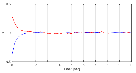
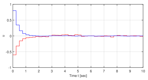
Figure 2: Trajectories of $x,u$ in the simulation of Example 1.

Example 2.

Consider the following dynamical model of the single-link robot arm given in [8]:

$$\dot{x}_{1}=x_{2},\;\dot{x}_{2}=-\sin(x_{1})+u+w,\;y=x_{1}.$$

The system can be written in the form of (47) with $A\!=\!\begin{pmatrix}0&1\\ 0&0\end{pmatrix}$, $B\!=\!\begin{pmatrix}0\\ 1\end{pmatrix}$, $C\!=\!(1,0)$, $E\!=\!\begin{pmatrix}0\\ -1\end{pmatrix}$, $E_{w}\!=\!\begin{pmatrix}0\\ 1\end{pmatrix}$, $q\!=\!x_{1}$, $C_{q}\!=\!(1,0)$, $p(q)\!=\!\sin(q)$. The nonlinearity $p$ is globally Lipschitz and satisfies the incremental quadratic constraint (48) with $M=\begin{pmatrix}1&0\\ 0&-1\end{pmatrix}$. Consider the configuration in Fig.1 (b). Assume that the continuous-time observer is (52) and the control input is (53). By the results of [30], $K_{1}=(-7.3936,-3.9937)$, $K_{2}=1$, $L_{1}=-1$, $L_{2}=\begin{pmatrix}-5.1294\\ -18.0352\end{pmatrix}$ can be chosen. By letting $\alpha=1.1$, the LMI (4.2) in Theorem 4 is solved, which yields the values of $a_{1},a_{2},b_{1},b_{2},\mu_{1},\mu_{2},d,\gamma_{1},\gamma_{2},c_{1},c_{2}$, from which $\mathcal{T}(\mu_{1},\gamma_{1})=0.0751,\mathcal{T}(\mu_{2},\gamma_{2})=0.0639$. Then, solve the LMI (58) to obtain the matrices $P_{1}=0.1462$ and $P_{2}=\begin{pmatrix}0.6307&0.1195\\ 0.1195&0.1434\end{pmatrix}$. Choose $h=0.02,s=0.02,\lambda_{1}=0.627,\lambda_{2}=0.575,\alpha_{0}=1$. By Theorem 4, the triggering functions are chosen as $\Gamma_{y}(y,y_{e})=0.9554\|y_{e}\|^{2}-0.02y^{\top}P_{1}y,\Gamma_{u}(\hat{x},x_{e})=1.1526\|x_{e}\|^{2}-0.02\hat{x}^{\top}P_{2}\hat{x}.$ Choose the initial state as $x_{1}(0)=-0.2,x_{2}(0)=0.6,\hat{x}_{1}(0)=-0.3,\hat{x}_{2}(0)=0.7$, and let the disturbance be randomly generated and satisfies $\|w\|_{\infty}\leq 0.05$. The simulation results are shown in Fig. 3, where the trajectories of $x$, $\hat{e}$ and $u$ are plotted. It can be seen that $x_{1},x_{2},\hat{e}$ all eventually go to a neighborhood of the origin in the presence of disturbances.

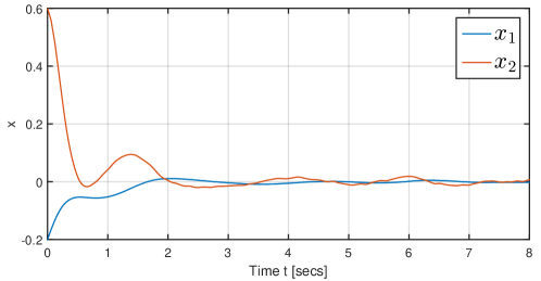
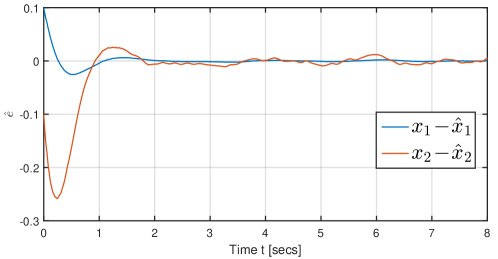
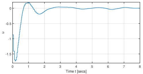
Figure 3: Trajectories of $x,\hat{x},u$ in the simulation of Example 2.

6 Conclusion

This paper investigated periodic event-triggered control design for nonlinear systems subject to disturbances using the impulsive system approach. Sufficient conditions were proposed to ensure the resulting closed-loop system input-to-state stable using state feedback and observer-based output feedback controllers, respectively. LMI-based sufficient conditions for the PETC design of incrementally quadratic nonlinear systems were also proposed. For all the cases considered, the sampling period and the triggering functions were given explicitly.

References

- [1] W. Heemels, K. H. Johansson, and P. Tabuada, “An introduction to event-triggered and self-triggered control,” in IEEE Conf. on Decision and Control, 2012, pp. 3270–3285.
- [2] P. Tabuada, “Event-triggered real-time scheduling of stabilizing control tasks,” IEEE Transactions on Automatic Control, vol. 52, no. 9, pp. 1680–1685, 2007.
- [3] Y. Shoukry and P. Tabuada, “Event-triggered state observers for sparse sensor noise/attacks,” IEEE Transactions on Automatic Control, vol. 61, no. 8, pp. 2079–2091, 2016.
- [4] X. Wang and M. D. Lemmon, “Event-triggering in distributed networked control systems,” IEEE Transactions on Automatic Control, vol. 56, no. 3, pp. 586–601, 2011.
- [5] E. Garcia and P. J. Antsaklis, “Model-based event-triggered control for systems with quantization and time-varying network delays,” IEEE Transactions on Automatic Control, vol. 58, no. 2, pp. 422–434, 2013.
- [6] D. Borgers and W. M. Heemels, “Event-separation properties of event-triggered control systems,” IEEE Transactions on Automatic Control, vol. 59, no. 10, pp. 2644–2656, 2014.
- [7] M. Donkers and W. Heemels, “Output-based event-triggered control with guaranteed -gain and improved and decentralized event-triggering,” IEEE Transactions on Automatic Control, vol. 57, no. 6, pp. 1362–1376, 2012.
- [8] M. Abdelrahim, R. Postoyan, J. Daafouz, and D. Nešić, “Robust event-triggered output feedback controllers for nonlinear systems,” Automatica, vol. 75, pp. 96–108, 2017.
- [9] ——, “Stabilization of nonlinear systems using event-triggered output feedback controllers,” IEEE Transactions on Automatic Control, vol. 61, no. 9, pp. 2682–2687, 2016.
- [10] W. H. Heemels, M. Donkers, and A. R. Teel, “Periodic event-triggered control for linear systems,” IEEE Transactions on Automatic Control, vol. 58, no. 4, pp. 847–861, 2013.
- [11] W. Heemels and M. Donkers, “Model-based periodic event-triggered control for linear systems,” Automatica, vol. 49, no. 3, pp. 698–711, 2013.
- [12] W. Heemels, R. Postoyan, M. Donkers, A. R. Teel, A. Anta, P. Tabuada, and D. Nešic, “Periodic event-triggered control,” Event-based control and signal processing, pp. 105–120, 2015.
- [13] A. Eqtami, D. V. Dimarogonas, and K. J. Kyriakopoulos, “Event-triggered control for discrete-time systems,” in American Control Conference, 2010, pp. 4719–4724.
- [14] S. Linsenmayer, D. V. Dimarogonas, and F. Allgöwer, “Periodic event-triggered control for networked control systems based on non-monotonic lyapunov functions,” Automatica, vol. 106, pp. 35–46, 2019.
- [15] L. Etienne, S. Di Gennaro, and J.-P. Barbot, “Periodic event-triggered observation and control for nonlinear lipschitz systems using impulsive observers,” International Journal Of Robust And Nonlinear Control, vol. 27, no. 18, pp. 4363–4380, 2017.
- [16] D. Borgers, R. Postoyan, A. Anta, P. Tabuada, D. Nešić, and W. Heemels, “Periodic event-triggered control of nonlinear systems using overapproximation techniques,” Automatica, vol. 94, pp. 81–87, 2018.
- [17] W. Wang, R. Postoyan, D. Nešić, and W. M. H. Heemels, “Stabilization of nonlinear systems using state-feedback periodic event-triggered controllers,” in IEEE Conf. on Decision and Control, 2016, pp. 6808–6813.
- [18] E. Aranda-Escolástico, M. Abdelrahim, M. Guinaldo, S. Dormido, and W. Heemels, “Design of periodic event-triggered control for polynomial systems: a delay system approach,” IFAC-PapersOnLine, vol. 50, no. 1, pp. 7887–7892, 2017.
- [19] J. Yang, J. Sun, W. X. Zheng, and S. Li, “Periodic event-triggered robust output feedback control for nonlinear uncertain systems with time-varying disturbance,” Automatica, vol. 94, pp. 324–333, 2018.
- [20] W. Wang, R. Postoyan, D. Nešsić, and W. Heemels, “Periodic event-triggered output feedback control of nonlinear systems,” in IEEE Conf. on Decision and Control, 2018, pp. 957–962.
- [21] W. Wang, R. Postoyan, D. Nesic, and W. Heemels, “Periodic event-triggered control for nonlinear networked control systems,” IEEE Transactions on Automatic Control, vol. 65, no. 2, pp. 620–635, 2020.
- [22] H. Khalil, Noninear Systems (3rd Edition). Prentice Hall, 2002.
- [23] J. P. Hespanha, D. Liberzon, and A. R. Teel, “Lyapunov conditions for input-to-state stability of impulsive systems,” Automatica, vol. 44, no. 11, pp. 2735–2744, 2008.
- [24] Y. Lin, E. Sontag, and Y. Wang, “Various results concerning set input-to-state stability,” in IEEE Conf. on Decision and Control, 1995, pp. 1330–1335.
- [25] S. Dashkovskiy and A. Mironchenko, “Input-to-state stability of nonlinear impulsive systems,” SIAM Journal on Control and Optimization, vol. 51, no. 3, pp. 1962–1987, 2013.
- [26] D. Carnevale, A. R. Teel, and D. Nesic, “A Lyapunov proof of an improved maximum allowable transfer interval for networked control systems,” IEEE Transactions on Automatic Control, vol. 52, no. 5, pp. 892–897, 2007.
- [27] D. Nesić, A. Teel, and D. Carnevale, “Explicit computation of the sampling period in emulation of controllers for nonlinear sampled-data systems,” IEEE Transactions on Automatic Control, vol. 54, no. 3, pp. 619–624, 2009.
- [28] E. D. Sontag, “Input to state stability: Basic concepts and results,” in Nonlinear and optimal control theory. Springer, 2008, pp. 163–220.
- [29] B. Açıkmeşe and M. Corless, “Observers for systems with nonlinearities satisfying incremental quadratic constraints,” Automatica, vol. 47, no. 7, pp. 1339–1348, 2011.
- [30] X. Xu, B. Açıkmeşe, and M. Corless, “Observer-based controllers for incrementally quadratic nonlinear systems with disturbances,” IEEE Transactions on Automatic Control, 2020. [Online]. Available: https://ieeexplore.ieee.org/document/9099370
- [31] A. Papachristodoulou, J. Anderson, G. Valmorbida, S. Prajna, P. Seiler, and P. Parrilo, “SOSTOOLS version 3.00 Sum of Squares optimization toolbox for Matlab,” arXiv:1310.4716, 2013. [Online]. Available: http://arxiv.org/abs/1310.4716