Automatised matching between two scalar sectors at the one-loop level

Abstract

Nowadays, one needs to consider seriously the possibility that a large separation between the scale of new physics and the electroweak scale exists. Nevertheless, there are still observables in this scenario, in particular the Higgs mass, which are sensitive to the properties of the UV theory. In order to obtain reliable predictions for a model which involves very heavy degrees of freedom, the precise matching to an effective theory is necessary. While this has been so far only studied for a few selected examples, we present an extension of the Mathematica package SARAH to perform automatically the matching between two scalar sectors at the full one-loop level for general models. We show that we can reproduce all important results for commonly studied models like split- or high-scale supersymmetry. One can now easily go beyond that and study new ideas involving very heavy states, where the effective model can either be just the standard model or an extension of it. Also scenarios with several matching scales can be easily considered. We provide model files for the MSSM with seven different mass hierarchies as well as two high-scale versions of the NMSSM. Moreover, it is explained how new models are implemented.

1 Introduction

The Standard Model (SM) of particle physics is a very successful theory which has been completed with the discovery of the Higgs boson at the Large Hadron Collider (LHC) Aad:2012tfa ; Chatrchyan:2012xdj . On the other side, there are observations like dark matter for which no viable candidate exists within the SM. While it has been expected that solutions to the open problems of the SM, like e.g. supersymmetry (SUSY), exist close to the electroweak scale, the LHC has not found any direct signal for new physics so far. Therefore, the possibility of a large gap between the electroweak (EW) and the scale of new physics has been studied more intensively in the recent years. The most prominent idea in this direction is ’split supersymmetry’ (split-SUSY) in which the SUSY scalars are much heavier than the SM particles and the SUSY fermions ArkaniHamed:2004fb ; Giudice:2004tc ; ArkaniHamed:2004yi . In this setup, most of the appealing properties of SUSY like gauge coupling unification and a dark matter candidate are kept, but the coloured particles are too heavy to be produced at the LHC. Mechanisms have been proposed how split-SUSY could arise from string theory Antoniadis:2006eb ; Antoniadis:2005em , and also the question of naturalness has been discussed Bhattacharyya:2012ct . Moreover, the ansatz of high-scale SUSY, i.e. that all SUSY particles are much heavier than the EW scale, is taken seriously nowadays Giudice:2011cg ; Bagnaschi:2014rsa . While it is widely believed that these models suffer from a large fine-tuning, it has pointed out that large SUSY scales can be combined with the relaxion mechanism to solve the big and the small hierarchy problem simultaneously Batell:2015fma . The idea of SUSY with very large mass scales is not restricted to the Minimal Supersymmetric extension of the SM (MSSM), but has also been applied to other SUSY models like the Next-to-MSSM (NMSSM) Zarate:2016jch or models with Dirac gauginos Unwin:2012fj ; Benakli:2013msa ; Dudas:2013gga ; Fox:2014moa ; Benakli:2015ioa .

Even if states beyond the SM (BSM) are too heavy to be produced at current colliders, they often still have an in-print in experimental results, see e.g. Refs. Arvanitaki:2005fa ; Ibe:2013oha . The precise measurement of the Higgs boson mass of $m_{h}=125.09$ GeV Aad:2015zhl at the LHC has added another very important constraint in this direction. Consequently, large efforts were put in a precise Higgs boson mass calculation in split- or high-scale SUSY Bernal:2007uv ; Arvanitaki:2012ps ; Giudice:2011cg ; Bagnaschi:2014rsa ; Vega:2015fna . The reason for this endeavour is that the commonly used fixed order calculations of the Higgs boson mass in SUSY models should only be applied in the case of a small separation between the EW scale and the SUSY scale. Otherwise, the presence of large logarithms introduces a large uncertainty in the prediction of the numerical value of $m_{h}$ Vega:2015fna ; Athron:2016fuq ; Staub:2017jnp ; Allanach:2018fif . This can be resolved either by the standard ansatz of an effective field theory (EFT) in which the heavy states are integrated out Sasaki:1991qu ; Carena:1995bx ; Haber:1990aw ; Haber:1996fp ; Carena:2000dp ; Carena:2000yi ; Carena:2001fw ; Espinosa:2001mm ; Gorbahn:2009pp ; Lee:2015uza , or by a hybrid method in which the fixed-order calculation is combined with the higher-order leading logarithms extracted from an EFT Hahn:2013ria ; Bahl:2017aev ; Bahl:2016brp ; Bahl:2018jom . In both cases, one needs to know how the couplings among the light states depend on the full theory. In terms of the EFT ansatz this means that the full model involving heavy and light states must be matched to an effective theory at the scale at which the heavy degrees of freedom are integrated out. The matching at leading order is straight-forward and the relations often can be read off from the tree-level Lagrangians of both models. However, tree-level relations are usually not sufficient to obtain the necessary precision in the Higgs boson mass prediction. Therefore, higher-order corrections are needed. Of course, the matching procedure at the full one-loop level is already much more time-consuming. Depending on the details of the full and effective model also several subtleties like infra-red divergences can occur as discussed in Ref. Braathen:2018htl .

In order to facilitate these studies, we have developed an automatised process to perform the matching between the scalar sectors of two renormalisable theories. This feature has been implemented in the Mathematica package SARAH Staub:2008uz ; Staub:2009bi ; Staub:2010jh ; Staub:2012pb ; Staub:2013tta and provides the functionality to obtain analytical expressions for the matching conditions at the one-loop level. Also the interface between SARAH and SPheno Porod:2003um ; Porod:2011nf has been extended to include the matching between an EFT and a UV-complete theory. In that way, one can obtain very quickly numerical predictions for the Higgs boson mass but also for all kind of other observables that concern the Higgs boson. It is worth to stress that this functionality is not restricted to split- or high-scale versions of the MSSM. A large variety of SUSY, but also non-SUSY models, with large BSM scales can be studied with the presented tool-chain. Also the considered EFT need not be the SM, but could be a singlet extension, a Two-Higgs-Doublet-Model (THDM), or an even more complicated model. Concerning the nature of the heavy states, we restrict our attention to heavy fermions and scalars. The implementation of integrating out heavy vector bosons at the one-loop level is reserved for future work. However, the low-energy EFT can still contain an extended gauge sector which is also matched at the one-loop level. Nevertheless, we will mainly concentrate in the given examples on the established MSSM scenarios because they offer the possibility to compare our generic approach with results available in the literature.

This paper is organised as follows. In Sec. 2 we explain our generic matching procedure. In Sec. 3 the new routines in SARAH are explained while a comparison with the literature is done in Sec. 4. We summarise in Sec. 5

2 Generic Matching between Two Scalar Sectors

2.1 General Ansatz

We consider a general, renormalisable gauge theory with a set of scalars $\{\phi_{i}\}$ and fermions $\{\psi_{i}\}$ charged under unspecified (sub-)sets of the theories gauge group. Without loss of generality, one can always assume that the scalars are real. The Lagrangian can be written as

$$\mathcal{L}_{UV}= \frac{1}{2}D_{\mu}\phi_{a}D^{\mu}\phi_{a}+\psi^{\dagger}_{a}\not{D}_{\mu}\psi_{a}+\mbox{Tr}\left(F_{\mu\nu,a}F^{\mu\nu}_{a}\right)$$

$$\hskip 28.45274pt-\frac{1}{4!}\lambda_{abcd}\phi_{a}\phi_{b}\phi_{c}\phi_{d}-\frac{1}{3!}\kappa_{abc}\phi_{a}\phi_{b}\phi_{c}-\frac{1}{2}m^{2}_{ab}\phi_{a}\phi_{b}-(M_{ab}\psi_{a}\psi_{b}+Y_{abc}\psi_{a}\psi_{b}\phi_{c}+\text{h.c.})\,,$$ (1)

where all gauge and representation indices have been suppressed. The covariant derivative $D^{\mu}$ and the gauge fields are chosen such that the field strength tensors $\{F^{\mu\nu}_{a}\}$ form diagonal kinetic terms (in case of multiple gauged U(1) groups). In the following it is always assumed that all gauge groups are broken near the scale of EW symmetry breaking. If particles with very different masses appear in such a theory, one can categorise the particle content into light fields ($\{\phi_{i}^{L}\},\{\psi_{i}^{L}\}$) and heavy fields ($\{\phi_{i}^{H}\},\{\psi_{i}^{H}\})$. The Lagrangian becomes

$$\mathcal{L}_{UV}=\mathcal{L}_{L}(\phi_{i}^{L},\psi_{i}^{L})+\mathcal{L}_{\rm mix}(\phi_{i}^{L},\psi_{i}^{L},\phi_{i}^{H},\psi_{i}^{H})+\mathcal{L}_{H}(\phi_{i}^{H},\psi_{i}^{H})\,.$$ (2)

Integrating out all heavy fields leads to an effective theory which contains only light degrees of freedom

$$\mathcal{L}_{EFT}= \frac{1}{2}D_{\mu}\phi^{L}_{a}D^{\mu}\phi^{L}_{a}+\psi^{L,\dagger}_{a}\not{D}_{\mu}\psi^{L}_{a}+\mbox{Tr}\left(F_{\mu\nu,a}F^{\mu\nu}_{a}\right)$$ (3)

$$-\frac{1}{4!}\tilde{\lambda}_{abcd}\phi^{L}_{a}\phi^{L}_{b}\phi^{L}_{c}\phi^{L}_{d}-\frac{1}{3!}\tilde{\kappa}_{abc}\phi^{L}_{a}\phi^{L}_{b}\phi^{L}_{c}-\frac{1}{2}\ \tilde{m}^{2}_{ab}\phi^{L}_{a}\phi^{L}_{b}$$

$$-(\tilde{M}_{ab}\psi^{L}_{a}\psi^{L}_{b}+\tilde{Y}_{abc}\psi^{L}_{a}\psi^{L}_{b}\phi^{L}_{c}+\text{h.c.})$$

$$+\mathcal{L}_{EFT}^{d>4}\,,$$

where the last line contains operators with dimension greater than four. Concerning a precise prediction of Higgs boson masses, only purely scalar operators with ascending dimensionality may be of interest for the matching. However, for $d>4$, their influence on the scalar potential is of the order $\nicefrac{{v_{i}}}{{M_{j}}}$, where $v_{i}$ is the vacuum expectation value (VEV) of a light and $M_{j}$ the mass of a heavy field, $v_{i}\ll M_{j}$. Supposed that the fundamental theory is renormalisable, it follows from the decoupling theorem, that the higher-dimensional operators become unimportant if $M_{j}\rightarrow\infty$. The question arises, at which scale the $\nicefrac{{v_{i}}}{{M_{j}}}$ terms are no longer relevant for a precise Higgs boson mass calculation. The impact of dimension-six terms, compared to ordinary threshold corrections ($d\leq 4$), on the Higgs boson mass in a matching of the SM to the MSSM was studied in Ref. Bagnaschi:2017xid . It was found that for $500\,\mathrm{GeV}<M_{j}<1000\,\mathrm{GeV}$, a two-loop matching of these operators yields corrections on $m_{h}$ in the sub-GeV range, which rapidly drop for $M_{j}>1\,\mathrm{TeV}$. Since the focus of this work is on BSM scenarios with $M_{j}\geqslant 1\,\mathrm{TeV}$, we neglect all $\nicefrac{{v_{i}}}{{M_{j}}}$ contributions during the matching. Thus, we assume that all VEVs responsible for the breaking of a low-energy gauge theory can be neglected compared to the masses of the heavy states. In particular, this means that all gauge bosons as well as chiral fermions are treated as massless in the computation of the matching conditions.

All information about the heavy states is encoded in the effective couplings and masses $\tilde{\lambda}$, $\tilde{\kappa}$, $\tilde{m}^{2}$, $\tilde{M}$ and $\tilde{Y}$. The purely scalar interactions $\tilde{\lambda}$, $\tilde{\kappa}$ and mass squared $\tilde{m}^{2}$ contain the crucial information about the scalar sector of the EFT, hence, they have the biggest impact on the properties of the light scalars. We know today, that (at least) one of these light scalars must have couplings comparable to the predictions of an SM-like Higgs boson and the mass must be about 125 GeV. Thus, even if the mass scale of the heavy fields is well above the reach of the LHC, we can test if the fundamental UV theory is consistent with the Higgs boson mass measurements through a precise calculation of the effective couplings at the matching scale and the Higgs properties at the weak scale. In order to determine the effective couplings in terms of parameters of the UV-theory, one assumes the matching condition that the $n$-loop $m$-point amplitudes involving the same external (light) states must yield the same result in the infra-red (IR) regime of the UV-theory (i.e. the scale where the heavy fields are integrated out) and the EFT,

$$\mathcal{M}^{(n)}(\phi^{L}_{a},\dots,\phi^{L}_{m})^{UV}=\mathcal{M}^{(n)}(\phi^{L}_{a},\dots,\phi^{L}_{m})^{EFT}\,.$$ (4)

Note, that the external fields in the two theories to be matched must be treated equally. Thus, additional wave-function renormalisations involing internal heavy fields may contribute to Eq. 4 by also matching the first derivative of the 2-point function w.r.t the external momentum of the light fields.

$$\begin{aligned} \includegraphics{FeynMF/FM_MatchTree1.pdf}\end{aligned}+\left(\begin{aligned} \includegraphics{FeynMF/FM_MatchTree2.pdf}\end{aligned}+t+u\right)$$

$$=\begin{aligned} \includegraphics{FeynMF/FM_MatchTree3.pdf}\end{aligned}+\left(\begin{aligned} \includegraphics{FeynMF/FM_MatchTree2.pdf}\end{aligned}+t+u\right)+\left(\begin{aligned} \includegraphics{FeynMF/FM_MatchTree4.pdf}\end{aligned}+t+u\right)$$

Figure 1: Matching of quartic couplings at tree-level. Light scalars are drawn with a single dashed line, heavy scalars with a double dashed line.

In this paper, we are going to calculate $\mathcal{M}$ using the Feynman diagrammatic approach neglecting all external momenta. The tree-level matching condition for a quartic coupling,

$$\tilde{\lambda}_{abcd}-\sum_{x\in\{\phi^{L}\}}\left(\frac{\tilde{\kappa}_{abx}\tilde{\kappa}_{xcd}}{m_{x}^{2}\to 0}+\frac{\tilde{\kappa}_{acx}\tilde{\kappa}_{xbd}}{m_{x}^{2}\to 0}+\frac{\tilde{\kappa}_{adx}\tilde{\kappa}_{xcb}}{m_{x}^{2}\to 0}\right) =\lambda_{abcd}$$

$$-\sum_{x\in\{\phi^{L}\}}\left(\frac{{\kappa}_{abx}{\kappa}_{xcd}}{m_{x}^{2}\to 0}+\frac{{\kappa}_{acx}{\kappa}_{xbd}}{m_{x}^{2}\to 0}+\frac{{\kappa}_{adx}{\kappa}_{xcb}}{m_{x}^{2}\to 0}\right)$$

$$-\sum_{x\in\{\phi^{H}\}}\left(\frac{{\kappa}_{abx}{\kappa}_{xcd}}{M_{x}^{2}}+\frac{{\kappa}_{acx}{\kappa}_{xbd}}{M_{x}^{2}}+\frac{{\kappa}_{adx}{\kappa}_{xcb}}{M_{x}^{2}}\right)\,,$$ (5)

is depicted in Fig. 1. Due to the assumption of vanishing external momenta and vanishing light masses, infra-red divergences appear on both sides of Eq. 5. Since the tree-level matching for cubic couplings is trivial,

$$\tilde{\kappa}_{abc}=\kappa_{abc}\,,$$ (6)

the divergences cancel exactly. Thus, the effective quartic couplings $\tilde{\lambda}_{abcd}$ are given by

$$\tilde{\lambda}_{abcd}= \lambda_{abcd}-\sum_{x\in\{\phi^{H}\}}\left(\frac{{\kappa}_{abx}{\kappa}_{xcd}}{M_{x}^{2}}+\frac{{\kappa}_{acx}{\kappa}_{xbd}}{M_{x}^{2}}+\frac{{\kappa}_{adx}{\kappa}_{xcb}}{M_{x}^{2}}\right)\,.$$ (7)

As already mentioned, the matching at tree level is not sufficient for a precise prediction of the properties of the scalar sector at the low-energy scale. Thus, one needs to include loop corrections changing the matching conditions to

$$\tilde{\kappa}_{abc}+\delta\tilde{\kappa}_{abc}(\phi^{L},\psi^{L})=\kappa_{abc}+\delta\kappa_{abc}(\phi^{L},\phi^{H},\psi^{L},\psi^{H})$$ (8)

$$\tilde{\lambda}_{abcd}-\sum_{x\in\{\phi^{L}\}}\sum_{\rm s,t,u}\frac{\tilde{\kappa}_{abx}\tilde{\kappa}_{xcd}}{m_{x}^{2}\to 0}+\delta\tilde{\lambda}_{abcd}(\phi^{L},\psi^{L}) =\lambda_{abcd}-\sum_{\rm s,t,u}\left(\sum_{x\in\{\phi^{L}\}}\frac{{\kappa}_{abx}{\kappa}_{xcd}}{m_{x}^{2}\to 0}+\sum_{x\in\{\phi^{H}\}}\frac{{\kappa}_{abx}{\kappa}_{xcd}}{M_{x}^{2}}\right)$$

$$\quad+\delta\lambda_{abcd}(\phi^{L},\phi^{H},\psi^{L},\psi^{H})\,,$$ (9)

where $\delta X(\phi^{L},\phi^{H},\psi^{L},\psi^{H})$, with $X=\lambda,\kappa$, denote the sum of all one-loop contributions that contain only light fields, mixed heavy and light fields as well as only heavy fields in the loop. Likewise $\delta\tilde{\lambda}$ can only arise from diagrams involving light fields in the loop since there are no heavy states present in the EFT. All generic diagrams which can contribute to tree-level and one-loop amplitudes of any renormalisable scalar operator are given in Appendix A. Again, IR divergences caused by light fields are present on both sides which need to cancel in the matching conditions. A detailed discussion on these cancellations is beyond the scope of this paper but was recently discussed in Ref. Braathen:2018htl . In summary, the matching condition can be expressed in terms of IR-finite pieces

$$\tilde{\kappa}_{abc} =\kappa_{abc}+\overline{\delta}\kappa_{abc}(\phi^{L},\phi^{H},\psi^{L},\psi^{H})$$ (10)

$$\tilde{\lambda}_{abcd} =\lambda_{abcd}-\sum_{x\in\{\phi^{H}\}}\sum_{\rm s,t,u}\left(\frac{{\kappa}_{abx}{\kappa}_{xcd}}{M_{x}^{2}}\right)+\overline{\delta}\lambda_{abcd}(\phi^{L},\phi^{H},\psi^{L},\psi^{H})\,,$$ (11)

where the one-loop contributions $\overline{\delta}X$ are computed using modified loop integrals where the IR divergent pieces have been subtracted. For instance, the scalar two-point integral $B_{0}$ with vanishing external momentum (for simplicity we omit the vanishing external momentum in the argument of all loop function) and vanishing masses suffers from a logarithmic IR divergence

$$B_{0}(m^{2},m^{2})|_{m^{2}\to 0}=\left.\log\left(\frac{Q^{2}}{m^{2}}\right)\right|_{m^{2}\to 0}\,$$ (12)

which will necessarily cancel in the matching condition Eq. 4. Thus, the replacement of the $B_{0}$ with the modified loop function

$$\left.\overline{B_{0}}(m^{2},m^{2})\right|_{m^{2}\to 0}=\left[B_{0}(m^{2},m^{2})-\log\left(\frac{Q^{2}}{m^{2}}\right)\right]_{m^{2}\to 0}$$ (13)

makes this cancellation manifest without the need to compute the corresponding IR-divergent diagrams in the EFT. Thus, the calculation of the matching conditions can be performed in a straight-forward way by using the IR-safe loop functions $\overline{B}_{0}$, $\overline{B}_{1}$, $\overline{C}_{0}$, $\overline{D}_{0}$, $\dot{\overline{B}}_{0}$ and $\dot{\overline{B}}_{1}$ defined in Appendix B.

2.2 Renormalisation Scheme

A simple renormalisation scheme which is applicable to a wide range of models is the $\overline{\text{MS}}$/$\overline{\text{DR}}$ scheme. Therefore, we are going to stick mainly to this scheme. The only exception is the treatment of the off-diagonal wave-function renormalisation (WFR) of the scalar fields. It has been proposed in Ref. Bagnaschi:2014rsa that these contributions can be dropped by assuming finite counter-terms for some input parameters. For instance, in the high-scale MSSM one could assume a counter-term for $\tan\beta$ which exactly cancels the off-diagonal WFR contributions. This approach is a more economic calculation and can lead to performance improvements in the runtime. However, it depends on the considered model and the chosen input parameters if such a scheme is possible. Therefore, we provide the possibility to include or exclude the one-loop contributions from off-diagonal WFR constants during the calculation.
For an appropriate choice of the WFR treatment it is worth to mention the equivalence between excluding the off-diagonal WFR constants and the extraction of effective quartic couplings from a pole-mass matching Braathen:2018htl ; Athron:2016fuq . Thus, for the comparison with tools that use a pole-mass matching, the inclusion of off-diagonal WFR constants should be disabled in the calculation.

2.3 Parametrisation of the Results at the Matching Scale

Figure 2: One-loop diagram contributing to the shift from $\overline{\text{MS}}$–$\overline{\text{DR}}$ conversion.

Using matching conditions to calculate the effective couplings yields solutions that are functions of the parameters of the UV theory. However, in some cases it might be better to (at least partially) give their dependence on the EFT parameters. This is especially the case for the SM gauge and Yukawa couplings because their values are known very precisely. Therefore, one also needs to match these couplings at a suitable loop-level. Concerning the matching of the scalar sector, the EFT parameters that enter the scalar matching conditions at tree-level need to be matched at the one-loop level (and re-inserted into the scalar tree-level matching). For all other parameters, a tree-level matching is sufficient as long as we stick to a one-loop matching of the scalar couplings. For non-supersymmetric models the scalar parameters which we want to match are free parameters, i.e. in these cases a matching of the SM parameters at tree-level is always sufficient. This is different for supersymmetric models because the scalar couplings are related to the other couplings through $F$- and $D$-terms. We concentrate on the $D$-term contributions, i.e. the matching of the gauge couplings, because this is the part important for the matching of scalars that could – at least in principle – provide a SM-like Higgs boson. The matching of the gauge couplings is parametrised by

$$g_{i}\to g_{i}+\delta g_{i}$$ (14)

and receives two different contributions:

1. Thresholds from heavy fields:

   $$\delta g_{i}=\sum_{\phi^{H}}\frac{1}{16\pi^{2}}\frac{C^{i}(\phi^{H})}{12}I_{2}^{i}(\phi^{H})g_{i}^{3}\log\frac{M_{\phi_{H}}^{2}}{Q^{2}}+\sum_{\psi^{H}}\frac{1}{16\pi^{2}}\frac{C^{i}(\psi^{H})}{3}I_{2}^{i}(\psi^{H})g_{i}^{3}\log\frac{M_{\psi_{H}}^{2}}{Q^{2}}\,,$$ (15)

   where $g_{i}$ is the gauge coupling with respect to the gauge group $i$, $I_{2}^{i}(x)$ is the Dynkin index of the field $x$ with respect to the gauge group $i$, and $C^{i}(x)$ is a multiplicity factor taking into account the charges under non-Abelian gauge groups others than $i$, i.e. in the case of the SM gauge group, this counts the colour and isospin multiplicity in the loop.

2. $\overline{\text{MS}}$–$\overline{\text{DR}}$ conversion: required if an $\overline{\text{MS}}$ and a $\overline{\text{DR}}$ renormalised quantity are to be matched. This is e.g. the case if non-SUSY models are matched onto SUSY ones. There are two different contributions which affect the quartic couplings:

   • The finite shifts of the gauge couplings for an $SU(N)$ group are Martin:1993yx

     $$\delta g_{i}=\frac{1}{16\pi^{2}}g_{i}^{3}\frac{N}{6}\,.$$ (16)

   • Quartic vertices receive an additional shift from $\overline{\text{MS}}$–$\overline{\text{DR}}$ conversion from the diagrams shown in Fig. 2. The amplitude difference of this diagram between the two schemes is

     $$\mathcal{M}=c_{1}c_{2}\,,$$ (17)

     where $c_{1}$ and $c_{2}$ are the two involved vertices between two scalars and two vector bosons.

The calculation of the two different contributions was implemented in SARAH and are automatically included in the matching procedure.

2.4 Above and Below the Matching Scale: Threshold Corrections to Fermionic Couplings

So far, we have concentrated on scenarios where the running above the matching scale can be neglected and the threshold corrections to fermionic couplings do not play an important role. Of course, there are plenty of situations where it is necessary to go beyond that. The simplest case is a high-scale SUSY scenario which is connected to a common SUSY breaking mechanism like minimal supergravity (mSugra). Such a SUSY breaking predicts that the masses of the sparticles are degenerate at the scale of grand unification (GUT), but not necessarily at the matching scale. Thus, finite differences between the running masses are present below the GUT scale. In such cases, one needs to consider the running above the matching scale up to the GUT scale. Since two-loop renormalisation group equations (RGEs) are commonly used for that running, it is necessary to include the threshold corrections to the SM gauge and Yukawa couplings. While the threshold corrections to the gauge couplings are given by Eq. 15 and Eq. 16, some more work is needed to compute the shifts to the Yukawa couplings. The general ansatz to calculate these shifts is the same as for the scalar couplings, i.e. imposing that the $n$-loop amplitudes of corresponding fields are identical at the matching scale $M_{M}$. Once again, all IR divergences must cancel at $M_{M}$, i.e. one determines the Yukawa couplings above the threshold scale via

$$Y_{abc}=\tilde{Y}_{abc}-\overline{\delta}Y_{abc}\;,$$ (18)

where $Y_{abc}$ is for instance a running SM Yukawa coupling and $\overline{\delta}Y_{abc}$ contains corrections from diagrams containing heavy fields, which are obtained with IR-safe loop functions, as well as $\overline{\text{MS}}$–$\overline{\text{DR}}$ conversion if necessary.
If the EFT is not the SM but an extension with additional fermions, also new Yukawa-like couplings are present below the matching scale. A good example for such a scenario is for instance split-SUSY with effective gaugino–Higgsino–Higgs couplings. Of course, the one-loop relation to calculate these couplings is just given by inverting Eq. 18, i.e.

$$\tilde{Y}_{abc}=Y_{abc}+\overline{\delta}Y_{abc}\;.$$ (19)

Thus, in a generic approach, both types of Yukawa coupling corrections, above (SM-like) and below (BSM-like) the matching scale are obtained simultaneously. Necessary ingredients are the one-loop diagrams depicted in Fig. 3 together with the wave-function corrections of the external states.

Figure 3: Irreducible one-loop diagrams contributing to the threshold corrections to scalar-fermion couplings. The diagram on the right only shows up for $\overline{\text{MS}}$–$\overline{\text{DR}}$ conversion.

3 Implementation in SARAH and SPheno

In the last section all necessary ingredients for a matching of two arbitrary renormalisable scalar sectors at the one-loop level were introduced. In this section we describe the implementation as well as the usage in the computer programs SARAH and SPheno.

3.1 General Information about SARAH and SPheno

SARAH is a Mathematica package optimised for an easy, fast and exhaustive study of BSM models. For a given model, which is defined in form of three input files, SARAH derives all tree-level properties, i.e. mass matrices, tadpole equations and vertices. Moreover, the analytical calculations of one-loop self-energies and tadpoles as well as of two-loop renormalisation group equations (RGEs) are fully automatised in SARAH based on generic results given in literature Machacek:1983tz ; Machacek:1983fi ; Machacek:1984zw ; Martin:1993zk ; Luo:2002ti ; Fonseca:2011vn ; Goodsell:2012fm ; Fonseca:2013bua ; Sperling:2013eva ; Sperling:2013xqa ; Schienbein:2018fsw . With version 3, SARAH became the first ’spectrum-generator-generator’: all analytical information derived by SARAH can be exported to Fortran code which provides a fully-fledged spectrum generator based on SPheno. A SARAH generated SPheno version calculates all masses at the full one-loop level, and includes the dominant two-loop corrections for neutral scalars Goodsell:2014bna ; Goodsell:2015ira ; Braathen:2017izn . Beyond that, SPheno makes predictions for two- and three-body decays, flavour and precision observables Goodsell:2017pdq ; Porod:2014xia , and the EW fine-tuning. In order to define the properties of the generated SPheno version, SARAH needs an additional input file usually called SPheno.m. This input contains the following information:

• The input parameters of the model

• The choice for the renormalisation scale

• The boundary conditions at the electroweak scale, at the renormalisation scale and at the GUT scale

• Optional: a condition to dynamically determine the GUT scale, e.g. $g_{1}(m_{\rm GUT})=g_{2}(m_{\rm GUT})$

• A list of particles for which the two- and three body decays should be calculated

Since the SPheno.m file will be important for the discussion in the following, we give an example in Appendix C how such a file may look like. For more details, we refer to the manual as well as the SARAH wiki page. In the following section, we discuss various aspects that arise in an automatised matching between two models and how they have been considered through the implementation of two independent approaches.

3.2 Available Options to Perform the Matching

The matching of two scalar sectors can be motivated by a precise investigation of very different properties of the theories to be matched. The largest contributions to threshold corrections often have their origin in one common sector of the heavy spectrum. It can be of particular interest to track this origin down in order to learn more about which parts of a given UV-theory are essential for the predictions in an EFT framework. For this purpose an analytical evaluation of threshold corrections is preferred. The analytical solutions can also easily be ported to other computer programs which is a key feature of many existing SARAH routines.

As already discussed, the matching of an EFT onto a UV-complete model does not only influence many low-energy observables but also enters the RGE running and other predictions above the matching scale. Considering the whole picture of the matching procedure and its numerical influence in all sectors of the theories to be matched, a numerical calculation of threshold corrections is preferred because it can easily be embedded into existing routines of the generated SPheno code.

With SARAH version 4.14.0 we provide two different possibilities to perform the matching between two arbitrary scalar sectors:

1. An analytical calculation within Mathematica

2. A fully numerical calculation using only the SPheno interface

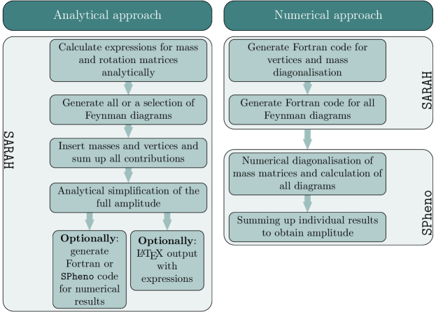
Figure 4: Schematic procedure for the two options to calculate matching conditions with SARAH/SPheno.

It is important to stress that both options are not based on the same routines, but have been implemented independently. Thus, they offer the possibility to double check the obtained results. A schematic comparison of the two approaches is given in Fig. 4. A summary of the description given here is also available at the SARAH wiki page.

For the analytical calculation it is necessary that all mass matrices in the model can be diagonalised analytically. Thus, it is usually necessary to work with a set of assumptions which simplify the most general mass matrices in a given model. In theories with spontaneous symmetry breaking, a high degree of different mixing patterns is introduced through the presence of VEVs. It has already been argued that, if these VEVs are responsible for the generation of masses in the EFT, i.e. if the low-energy Lagrangian is invariant under the symmetries broken by these VEVs, a common assumption is to neglect all small VEVs. In addition, flavour violating effects are usually negligible. The only exception are scenarios in which large contributions to flavour violation occur in the new physics sector. This could for instance happen in the MSSM with large off-diagonal trilinear soft-terms which can have a big effect on the Higgs boson mass Goodsell:2015yca . Thus, if any of these assumptions is not justified, it is necessary to switch to the purely numerical calculation.

Although the focus of the Mathematica interface is on the derivation of analytical expressions for the matching conditions, additional routines have been implemented to make these results easily usable in numerical calculations. This has the advantage that the obtained code for numerical evaluations can be much faster than the fully numerical interface because many simplifications can be performed on the analytical level. In addition, the obtained results can be exported into LaTeX files which makes a evaluation of the expressions in a human readable format possible. On the other hand, the fully numerical implementation has several advantages: (i) the RGE running above the matching scale can be performed, (ii) shifts to fermionic couplings can be included, (iii) several EFTs appearing in models with more than one matching scale can be automatically linked (iv) flavour violating effects can be included.

Before describing the user interface of the new routines, we want to comment on a few subtleties to provide a better understanding on the importance of certain user inputs.

1. Model files: in principle, one can set up specific model files for the UV theory where for instance EW VEVs are dropped from the very beginning. However, this complicates further studies of the UV theory. Thus, we are going to work in the following with the default model files delivered with SARAH. For instance, we use the MSSM implementation which includes EW VEVs and apply the simplifying assumption to neglect these VEVs during the matching procedure. However, the considered EFT may require the development of further model files. For instance, various split-SUSY models that contain only the fermionic degrees of freedom of their corresponding SUSY models already have been implemented in the new SARAH version.

2. Normalisation of couplings: in many models studied in literature, the coefficients in front of the scalar couplings are often chosen differently from Eq. 1. For instance, a common convention for the SM Lagrangian reads

   $$\mathcal{L}_{SM}=\left(D_{\mu}H\right)\left(D^{\mu}H\right)^{\dagger}+\sum_{f}\bar{f}\not{D}f-\left(\frac{1}{2}\lambda_{SM}|H|^{4}+\mu^{2}|H|^{2}\right)-\left(Y_{d}H^{\dagger}\bar{d}q+Y_{e}H^{\dagger}\bar{e}l-Y_{u}H\bar{u}q+\text{h.c.}\right)$$ (20)

   Thus, after replacing $H^{0}\to\frac{1}{\sqrt{2}}\left(h+iG+v\right)$ the vertex in Eq. 1 between four Higgs fields $h$ is

   $$\tilde{\kappa}_{hhhh}=-3\lambda_{SM}\,.$$ (21)

   Therefore, the correct matching condition to calculate $\lambda_{SM}$ becomes

   $$\lambda_{SM}=-\frac{1}{3}\left(\kappa_{hhhh}+\bar{\delta}\kappa_{hhhh}+\sum_{s,t,u}\,\sum_{x\in\{\phi^{H}\}}\frac{\left(\kappa_{hhx}\right)^{2}}{M_{x}^{2}}\right)\,,$$ (22)

   where $\kappa_{i}$ denotes tree-level vertices in the UV theory while $\bar{\delta}$ are the corresponding one-loop shifts. The relative normalizations between operators in the considered UV and the effective theory, such as for example the factor $-\nicefrac{{1}}{{3}}$ in Eq. 22, have to be provided by the user.

3. Superposition of fields: when matching a scalar sector involving multiple (light) scalar fields with identical quantum numbers, often linear combinations of external fields contribute to the matching of different parameters. For instance, consider the couplings $\lambda_{4}$ and $\lambda_{5}$ in a THDM:

   $$\mathcal{L}_{THDM}=\dots-\lambda_{4}|H_{1}^{\dagger}H_{2}|^{2}-\frac{1}{2}\left(\lambda_{5}(H_{1}^{\dagger}H_{2})^{2}+\text{h.c.}\right)\,,$$ (23)

   where the two $SU(2)$ doublets $H_{1}$ and $H_{2}$ have the same hypercharge. We find that any vertex involving $\lambda_{4}$ receives also contributions from $\lambda_{5}$ and vice versa. For instance consider the couplings

   $$\kappa_{h_{1}h_{2}H_{1}^{+}H_{2}^{-}}=-\frac{1}{2}\left(\lambda_{4}+\lambda_{5}\right)\,,$$ (24)

   $$\kappa_{h_{1}A_{2}H_{1}^{+}H_{2}^{-}}=\frac{1}{2}i\left(\lambda_{4}-\lambda_{5}\right)\,,$$ (25)

   after splitting the two doublets into their charged ($H^{\pm}_{1,2}$), CP-even ($h_{1,2}$) and CP-odd ($A_{1,2}$) components (note that the gauge eigenstates introduced here also correspond to the mass eigenstates as we assume vanishing VEVs). For simplicity, we assume real parameters . Thus, to obtain the matching conditions for $\lambda_{4}$ and $\lambda_{5}$ separately, it is necessary to calculate the superpositions

   $$\lambda_{4}=-\left(\mathcal{M}(h_{1}h_{2}H_{1}^{+}H_{2}^{-})+i\mathcal{M}(h_{1}A_{2}H_{1}^{+}H_{2}^{-})\right)\,,$$ (26)

   $$\lambda_{5}=-\left(\mathcal{M}(h_{1}h_{2}H_{1}^{+}H_{2}^{-})-i\mathcal{M}(h_{1}A_{2}H_{1}^{+}H_{2}^{-})\right)\,.$$ (27)

   These conditions are user input as well.

3.3 Analytical Approach

In order to use the Mathematica interface to obtain analytical expressions for the matching conditions, one needs to initialize a Mathematica kernel, load SARAH and start the considered high-scale model. This can be done by opening a new Mathematica notebook and entering the commands

⬇

In[1]Start["<Model>"]

where <Model> could be for instance MSSM or NMSSM. In the next step, there are two possibilities to obtain the matching conditions analytically:

1. one can calculate individual effective couplings in an interactive mode or

2. use a batch mode to calculate several matching conditions at once and to optionally obtain LaTeX , Fortran and SPheno outputs.

We are going to give details about both options which are based on the new command

⬇

InitMatching[Options]

where possible options are

• Parametrisation -> $LIST

  • Default: {}

  • Description: list of specific parametrisations of selected model parameters

  • Example: {vu -> v Sin[ArcTan[TanBeta]], ...}

• Assumptions -> $LIST

  • Default: {}

  • Description: list of assumptions for parameters in the model in order to simplify the expressions

  • Example: {TanBeta>0}

• SolveTadpoles -> $LIST

  • Default: {}

  • Description: list of parameters which are obtained by the tadpole equations

  • Example: {mHu2,mHd2}

• ReadLists -> $BOOL

  • Default: False

  • Description: if set to True, the calculation of vertices is skipped, but results stored in a previous session are used. This can be a significant performance boost.

• InputFile -> $FileName

  • Default: False

  • Description: can be used to define an input file containing all necessary information

A short description of this command can be obtained within a SARAH session by invoking the command ?InitMatching.

If the interactive mode is demanded, the option InputFile has to be omitted while values for Parametrisation, Assumptions and SolveTadpoles should be provided to allow for an analytical diagonalization of all mass matrices. The usage of the batch mode requires only the option InputFile and serves a high reproducibility of the obtained results by providing only one single input file.

The provided assumptions and parametrisations are used to calculate analytical expressions for all masses and rotation matrices. If this is not possible, because Mathematica cannot diagonalize the mass matrices analytically (using the build-in functions Eigensystem and SingularValueDecomposition), one can either use the purely numerical interface explained in Sec. 3.4 or choose appropriate simplifying assumptions.

3.3.1 Interactive Mode: Calculating Individual Matching Conditions

Initializing the matching routines using the InitMatching function with the options described in the previous paragraph while not specifying the option InputFile enables the interactive mode. The necessary vertices of the high-scale theory are calculated or loaded from a previous session and the masses/rotation matrices are derived. However, no further calculations are performed at this point.

Example initialization: consider a high-scale MSSM scenario where all SUSY particles have a degenerate mass MSUSY while only the SM Higgs remains light. A possible parametrisation may look like

⬇

In[3]MyParametrisation = {
vd -> v Cos[ArcTan[TanBeta]],
vu -> v Sin[ArcTan[TanBeta]],
v -> epsUV,
g1 -> g1Q,
g2 -> g2Q,
g3 -> g3Q,
Yu[a_,b_] :> 1/Sin[ArcTan[TanBeta]]*Delta[3,b]Delta[a,3]YuQ[a,b],
Yd[a_,b_] :> 1/Cos[ArcTan[TanBeta]]*Delta[3,b]Delta[a,3]YdQ[a,b],
Ye[a_,b_] :> 1/Cos[ArcTan[TanBeta]]*Delta[3,b]Delta[a,3]YeQ[a,b],
T[Yu][a__] :> Delta[a] At Yu[a],
T[Yd][a__] :> Delta[a] Ab Yd[a],
T[Ye][a__] :> Delta[a] Ae Ye[a],
mq2[a__] :> Delta[a] MSUSY^2,
mu2[a__] :> Delta[a] MSUSY^2,
md2[a__] :> Delta[a] MSUSY^2,
me2[a__] :> Delta[a] MSUSY^2,
ml2[a__] :> Delta[a] MSUSY^2,
conj[x_] -> x,
MassB -> MSUSY,
MassWB -> MSUSY,
MassG -> MSUSY,
\[Mu] -> MSUSY,
B[\[Mu]] -> MSUSY^2
};

Note that the symbols MSUSY, At, Ab, Ae and TanBeta are not defined in the MSSM model file. Thus, additional information about these symbols must be provided using the Assumptions option, otherwise they are assumed to be arbitrary complex numbers. The initialization is invoked by

⬇

In[4]InitMatching[Parametrisation->MyParametrisation,
SolveTadpoles->{mHd2,mHu2},
Assumptions -> {TanBeta > 0, MSUSY > 0, At>0, Ab>0, Ae>0}]

There are a few important comments concerning the parametrisation which we have used in this example:

• The symbol epsUV is used to indicate dimensionful parameters X which are to be neglected in the UV theory. One should always use this parameter instead of the simpler rule X->0 to avoid problems caused by a division by 0.

• It is recommended to express all matching conditions in terms of the running parameters of the effective theory, see Sec. 2.3. Therefore, we express the MSSM gauge and Yukawa couplings by the SM ones using the suffix Q which marks the running parameters (instead of g1 we e.g. specify it to be g1Q). For these parameters, only the tree-level matching conditions are required. The one-loop matching conditions for the gauge couplings, discussed in Sec. 2.3, are automatically derived.

• Delta[a,b] is the SARAH internal symbol for the Kronecker delta $\delta_{ab}$. We use it here to include only contributions from third generation Yukawa couplings, and to force diagonal soft masses for the sfermions.

• In order to simplify the analytical calculation, we assume that all parameters are real. This is translated by conj[x_]->x. The object conj is the SARAH internal command for complex conjugation.

When all calculations are finished, it is possible to validate if the obtained mass spectrum at the matching scale is as expected

⬇

In[5]?M

which yields the result

⬇

Out[5]      M[Ah]={0,MSUSY}
M[Cha]={MSUSY,MSUSY}
M[Chi]={-MSUSY,MSUSY,MSUSY,MSUSY}
M[Fd]={0,0,0}
M[Fe]={0,0,0}
M[Fu]={0,0,0}
M[Glu]=MSUSY
M[hh]={0,MSUSY}
M[Hpm]={0,MSUSY}
M[Sd]={MSUSY,MSUSY,MSUSY,MSUSY,MSUSY,MSUSY}
M[Se]={MSUSY,MSUSY,MSUSY,MSUSY,MSUSY,MSUSY}
M[Su]={MSUSY,MSUSY,MSUSY,MSUSY,MSUSY,MSUSY}
M[Sv]={MSUSY,MSUSY,MSUSY}

As expected, the spectrum at the matching scale contains one massless CP-even Higgs boson which corresponds to the SM-like Higgs boson. Also all SM-like fermions remain massless while the heavy fields are degenerate in the mass parameter MSUSY.
The rotation matrices are stored in the array ReplacementRotationMatrices and read in our example

⬇

{ZD[a__Integer] -> {{1, 0, 0, 0, 0, 0}, {0, 1, 0, 0, 0, 0}, {0, 0, 1, 0, 0, 0}, {0, 0, 0, 1, 0, 0}, {0, 0, 0, 0, 1, 0}, {0, 0, 0, 0, 0, 1}}[[a]],

...

ZH[a__Integer] -> {{1/Sqrt[1 + TanBeta^2], 1/Sqrt[1 + TanBeta^(-2)]}, {-(TanBeta/Sqrt[1 + TanBeta^2]), 1/Sqrt[1 + TanBeta^2]}}[[a]],

ZA[a__Integer] -> {{-(1/Sqrt[1 + TanBeta^2]), 1/Sqrt[1 + TanBeta^(-2)]}, {TanBeta/Sqrt[1 + TanBeta^2], 1/Sqrt[1 + TanBeta^2]}}[[a]],

ZP[a__Integer] -> {{-(1/Sqrt[1 + TanBeta^2]), 1/Sqrt[1 + TanBeta^(-2)]}, {TanBeta/Sqrt[1 + TanBeta^2], 1/Sqrt[1 + TanBeta^2]}}[[a]],

ZN[a__Integer] -> {{0, 0, 1/Sqrt[2], 1/Sqrt[2]}, {0, 0, -(1/Sqrt[2]), 1/Sqrt[2]}, {0, 1, 0, 0}, {1, 0, 0, 0}}[[a]],

...}

Let us now continue with the description of the analytical interface. After the successful initialization and calculation of all mass and rotation matrices, one can compute the leading order (LO) and next-to leading order (NLO) corrections to an amplitude with the external fields given in the list fieldlist

⬇

EFTcoupLO[fieldlist, Options]

EFTcoupNLO[fieldlist, Options]

The fieldslist can contain two, three or four scalar fields including their generation indices to obtain effective mass parameters and cubic or quartic couplings. Note that the matching of effective mass parameters is only demanded if no spontaneous symmetry breaking occurs in this sector of the theory. The possible options for the function EFTcoupNLO are

• Topologies -> $LIST

  • Default: {}

  • Description: list of topologies to include into the calculation. If empty, all topologies are used. Topologies are denoted as in Appendix A.

  • Example: {B[4][1],B[4][2][1], B[4][2][2]} or equivalently {B[4]}.

• ExcludeTopologies -> $LIST

  • Default: {OffdiagonalWFRs}

  • Description: list of topologies to be excluded from the calculation. The filtering of ExcludeTopologies is also applied on the topology groups given in the Topologies option, e.g. if {B[4]} is given in the Topologies list but B[4][2][2] in the ExcludeTopologies list, then only B[4][1] and B[4][2][1] are computed.

  • Example: {OffdiagonalWFRs, DiagonalWFRS} to exclude all contributions on external legs.

• ExcludeFields -> $LIST

  • Default: {}

  • Description: list of fields to be excluded when appearing as internal fields.

  • Example: {Cha,Chi} e.g. to exclude electroweakinos within a split SUSY scenario.

• InternalPatterns -> $LIST

  • Default: {}

  • Description: compute only diagrams with certain internal field-type patterns. For an empty list all patterns are computed.

  • Example: {S,SS,SSS,SSSS} computes corrections from heavy scalars only while {FF} computes diagrams that contain exactly two internal fermions.

• GaugeThresholds->$BOOL

  • Default: True

  • Description: whether to include the contributions from one-loop gauge coupling thresholds to the tree-level amplitude or not

• ShiftMSDR-> 0/1/2/Automatic

  • Default: Automatic

  • Description: whether to include the $\overline{\text{MS}}-\overline{\text{DR}}$ conversion factors. 0: no, 1: inclusive, 2: exclusive, Automatic: decide between 1 and 0 depending on the type of considered model (SUSY or non-SUSY). exclusive means that only the conversion factor is calculated while inclusive gives the full result plus conversion factor (default for SUSY models).

• Debug -> $BOOL

  • Default: False

  • Description: multiplies each amplitude with a debug variable marking its topology and field insertion

  • Example: the term debug[C[4][1]][hh[2],hh[2],hh[2]] may be multiplied with the expression of the amplitude of the triangle diagram (C[4][1], see Eq. 56) with three heavy internal Higgs bosons (hh[2],hh[2],hh[2]).

• SimplifyResults -> $BOOL

  • Default: True

  • Description: whether to simplify the results using the given assumptions or not.

• LoopReplace -> $FUNCTION

  • Default: AnalyticLoopFunctions

  • Description: the amplitudes contain loop functions in the FormCalc notation (e.g. a $B_{0}(0,m_{1}^{2},m_{2}^{2})$ function is denoted by B0i[bb0,0,m1^2,m2^2]). The function AnalyticLoopFunctions replaces them with the IR-save loop functions defined in Appendix B. However, for a better readability one may set this to the Identity function.

  • Example: Identity

To view a short description of the options within a SARAH session one can invoke the commands ?EFTcoupNLO and Options[EFTcoupNLO]. The function EFTcoupLO only provides the options SimplifyResults, Debug and ExcludeFields.

Example calculation: proceeding with the high-scale MSSM example i.e. the MSSM $\to$ SM matching we can use the introduced functions to calculate the expressions for the effective quartic coupling $\lambda_{SM}$ of the SM Higgs boson at the matching scale. The tree-level matching condition is calculated as follows

⬇

In[7]-1/3 EFTcoupLO[{hh[1],hh[1],hh[1],hh[1]}]

the output reads

⬇

Out[7](((g1Q^2 + g2Q^2) (-1 + TanBeta^2)^2)/(4 (1 + TanBeta^2)^2))

where the number in the square brackets denotes the generation index of the Higgs field hh. Note the coefficient $-\frac{1}{3}$, which we have included to get the value for $\lambda_{SM}$ as explained at the end of Sec. 3.2. Thus, we found at leading order

$$\lambda^{(\rm LO)}_{SM}=\frac{1}{4}(g_{1}^{2}+g_{2}^{2})\frac{(\tan^{2}\beta-1)^{2}}{(\tan^{2}\beta+1)^{2}}\,.$$ (28)

The full expression at the one-loop order is rather lengthy. Therefore, we make a few approximations and include only the terms involving the top quark Yukawa coupling. This can be achieved by setting all other couplings to zero. The command

⬇

In[8]-1/3 EFTcoupNLO[{hh[1],hh[1],hh[1],hh[1]}]//.{g1Q->0, g2Q->0, YeQ[3,3]->0, YdQ[3,3]->0, At -> (Xt + MSUSY/TanBeta)}

where we have introduced the stop mixing parameter $X_{t}=A_{t}-\mu\tan^{-1}\beta$, yields

⬇

Out[8]((12 MSUSY^2 Xt^2 - Xt^4 -12 MSUSY^4 Log[UVscaleQ^2/MSUSY^2]) YuQ[3,3]^4)/(32 MSUSY^4 Pi^2)

where the symbol UVscaleQ is the name for the renormalisation scale used in the loop functions. Note, because of the assumption $g_{i}\to 0$ this corresponds only to the leading one-loop shift but not to the full NLO expression (including the tree-level contributions), i.e. we found

$$\delta\lambda^{(\rm NLO)}_{SM}=\frac{Y_{t}^{4}}{32\pi^{2}}\left(\frac{12X_{t}^{2}}{M_{\rm SUSY}^{2}}-\frac{X_{t}^{4}}{M_{\rm SUSY}^{4}}\right)-\frac{3Y_{t}^{4}}{8\pi^{2}}\log\frac{Q_{match}^{2}}{M_{\rm SUSY}^{2}}\,,$$ (29)

which is the well-known leading one-loop shift maximized for $X_{t}=\sqrt{6}M_{\rm SUSY}$.

Advanced Examples: the root directory of the new SARAH version includes the file

Example_Matching.nb

which contains already evaluated Cells that describe the example usage of all possible Options of EFTcoupNLO (e.g. the selection of specific topologies or debugging) within the high-scale MSSM.

3.3.2 Batch Mode

The complexity of the calculation requires a high degree of reproducibility of the results. For this purpose it is possible to write input files that contain all necessary information for the matching to a given EFT model. This includes all information already discussed in the interactive mode. In addition, the correspondence between effective couplings in the low-energy model and amplitudes in the UV model, as it was demonstrated for the THDM matching, have to be defined.

The batch mode is invoked during the initialisation by specifying the input file <FileName> located in the directory of the loaded SARAH model

⬇

InitMatching[InputFile-><FileName>]

The mandatory content of the input file is

Matching.m

⬇

1$NameUV= "STRING" ;

2$ParametrisationUV = { … };

3$AssumptionsMatching={ … }

4$SolveTadpolesUV = { … };

5$MatchingConditions = {

6 {Parameter1, coefficient field1.field2.field3.field4},

7 …

8 {Parameter2, coefficient field1.field2.field3}

9 }

The purpose of the different keywords is

• $NameUV: defines a name for the current setup. This also determines the name of the output directory in which the results are saved into as well as the file name of the SPheno binary.

• $ParametrisationUV: the parametrisation in the UV. This is equivalent to option Parametrisation when running InitMatching without an input file.

• $SimplificationsMatching: a list of simplifications which are only applied at the matching scale.

• $AssumptionsMatching: a list of assumptions at the matching scale equivalent to the Assumptions option when running InitMatching without input file.

• $SolveTadpolesUV: the equivalent to the option SolveTadpoles of InitMatching.

• $MatchingConditions: a list of matching conditions which relates a parameter in the EFT to amplitudes in the high-scale model containing light external fields only, similar to Eqs. 26 and 27.

Up to $NameUV and $MatchingConditions this is the same information which is otherwise passed to InitMatching and EFTcoupLO/EFTcoupNLO in the interactive mode. In addition, one can define options to control the generation of LaTeX or SPheno output. This is described in more detail below. First, consider an input file example which defines a high-scale SUSY scenario

Matching_SimpleHighScaleSUSY.m

⬇

1$NameUV="SimpleHighScaleSUSY";

2

3$ParametrisationUV = {

4 vd -> v Cos[ArcTan[TanBeta]],

5 vu -> v Sin[ArcTan[TanBeta]],

6 v -> epsUV,

7 … (* as in the interactive mode *)

8 \[Mu]->MSUSY

9 };

10

11$SimplificationsMatching={

12 UVscaleQ->MSUSY,

13 conj[x_] :> x

14};

15

16$AssumptionsMatching={

17 TanBeta>0,

18 MSUSY>0

19}

20

21$SolveTadpolesUV = {mHd2, mHu2};

22

23$MatchingConditions = {

24 \[Lambda] -> -1/3 hh[1].hh[1].hh[1].hh[1]

25 };

Here, we skipped most of the lines for $ParametrisationUV because they are similar to the definition of MyParametrisation in the last subsection. For simplicity, we set here all trilinear sfermion couplings as well as the matching scale UVscaleQ equal to MSUSY.

If the option InputFile->"Matching_SimpleHighScaleSUSY.m" is given to InitMatching, SARAH will calculate all matching conditions defined in $MatchingConditions. The information is stored in the arrays

⬇

SA‘MatchingResultsLO

SA‘MatchingResultsNLO

and is also written to the destination directory

$SARAH_Directory/Output/$Model/EWSB/Matching/$NameUV

Thus, one can work with the results within other Mathematica sessions as well.

LaTeX  Output

One can use the batch mode to obtain LaTeX files which give information about calculated masses, rotation matrices and matching conditions in a human readable format. In order to produce this output, the input file must contain additional information which maps the additional symbols onto LaTeX symbols

Matching.m

⬇

11$EFTcouplingsToTeX = True;

12$AdditionalTeXsymbols={ … };

The meaning of these lines is

• $EFTcouplingsToTeX: if set to True, all information obtained during the matching is exported into a LaTeX file ready to be compiled by standard LaTeX compilers.

• $AdditionalTeXsymbols: a list containing replacement rules that define the correspondence between LaTeX and Mathematica  expressions which are for instance used in the defined parametrisation. This will improve the readability of the LaTeX document significantly.

Thus, for our chosen example, the entries might read

Matching_SimpleHighScaleSUSY.m

⬇

26$EFTcouplingsToTeX=True;

27$AdditionalTeXsymbols={

28 {\[Lambda], "\\lambda"},

29 {TanBeta, "t_{\\beta}"},

30 {MSUSY, "M_{\\text{SUSY}}"},

31 {g1Q, "g_1^{\\rm MS}"},

32 {g2Q, "g_2^{\\rm MS}"},

33 {g23, "g_3^{\\rm MS}"},

34 {YuQ[3,3], "Y_t^{\\rm MS}"},

35 {YdQ[3,3], "Y_b^{\\rm MS}"},

36 {YeQ[3,3], "Y_\\tau^{\\rm MS}"}

37};

where the additional backslash is a necessary escape character. The LaTeX files are saved in the same directory $SARAH_Directory/Output/$Model/EWSB/Matching/$NameUV as the other outputs.

SPheno output

With little effort, it is also possible to generate a SPheno version which includes the analytical matching conditions to be used within an iterative running between the matching and the EW scale. In order to do so, two steps are necessary:

1. Export the Mathematica expressions into Fortran code and write a corresponding SPheno.m file

2. Run the EFT model using this SPheno.m

The first step is again steered through the input file of InitMatching by adding the following information

Matching_SimpleHighScaleSUSY.m

⬇

38$ExportToSPheno=True;

39$SPhenoEFTmodel="SM";

40$SPhenoMINPAR={

41 {1, MSUSY},

42 {2, TanBeta}};

43$SPhenoBoundaryHighScale={};

44$SPhenoBoundaryRenScale={};

45$SPhenoTadpoles={mu2};

46$SPhenoMatchingScale={MSUSY};

47$SPhenoRenScale=173.;

48$SPhenoMatchingEWSB=Default[OHDM];

The export into SPheno routines is enabled with the first line. This option is sufficient to obtain Fortran routines for all matching conditions at the one-loop level. All other information must be given to automatically generate a suitable SPheno.m for the EFT model. Most variables have a 1:1 correspondence to the standard variables (without the $SPheno prefix) used in SPheno.m files discussed in Appendix C. The new option is $SPhenoMatchingScale which defines at which scale the matching should be performed.
Running InitMatching with an input file containing these lines, produces two outputs:

• The file EFTcoupling1_SPhenoEFT_MSSM_SimpleHighScaleSUSY.f90, located in the output directory of the MSSM model, which contains the matching conditions in Fortran format

  ⬇

  1Real(dp) Function EFTcoupling1(g1Q,g2Q,TanBeta,YdQ,YeQ,YuQ,UVscaleQ)

  2Implicit None

  3Complex(dp),Intent(in) :: YdQ(:,:),YeQ(:,:),YuQ(:,:)

  4Real(dp),Intent(in) :: g1Q,g2Q,TanBeta,UVscaleQ

  5

  6EFTcoupling1=-(-2*g2Q**4*TanBeta**4 + … &

  7 & )/(192._dp*Pi**2*TanBeta**4*(1 + TanBeta**2)**2)

  8

  9End Function EFTcoupling1

  where most of the terms in the sum have been omitted as they are not important for the discussion.
  

• a Mathematica file named SPhenoEFT_MSSM_SimpleHighScaleSUSY.m which is located in the model directory of the SM. This file may look like

  ⬇

  1ModelName = "SimpleHighScaleSUSY";

  2OnlyLowEnergySPheno = False;

  3MINPAR={{1, MSUSY}, {2, TanBeta}}

  4ParametersToSolveTadpoles={mu2}

  5UseParameterAsGUTscale = {{MSUSY}};

  6

  7RenormalizationScaleFirstGuess = 173.^2;

  8RenormalizationScale = 173.;

  9

  10DEFINITION[MatchingConditions]= Default[OHDM];

  11BoundaryHighScale = {};

  12BoundaryRenScale = {};

  13

  14BoundaryMatchingUV = {

  15{\[Lambda],EFTcoupling1[g1,g2,TanBeta,Yd,Ye,Yu,mGUT]}

  16};

  17

  18ListDecayParticles = Automatic;

  19ListDecayParticles3B = Automatic;

  20

  21RealParameters = {MSUSY, TanBeta};

  22

  23SelfDefinedFunctions = {

  24 ReadString["$SARAH_Directory/Output/MSSM/EWSB/Matching/SimpleHighScaleSUSY/\

  25 EFTcoupling1_SPhenoEFT_MSSM_SimpleHighScaleSUSY.f90"]

  26};

  One can see that this file contains the information given to InitMatching (line 1-12). In addition, the information about the matching and the corresponding Fortran routines (using parameter without the Q prefix) have been automatically added by SARAH (line 14-16 and 21-26).

The second step to generate a numerical code that includes the computed matching conditions is to run a new Mathematica kernel and call the SARAH routine MakeSPheno using the generated SPheno.m, i.e.

⬇

In[1]Start["SM"];

In[2]MakeSPheno[InputFile->"SPhenoEFT_MSSM_HighScaleSUSY.m"]

This generates all necessary Fortran routines for the high-scale SUSY implementation. The code is compiled in the same way as other SARAH generated SPheno modules:

1. Copy the SARAH output to a new sub-directory of your SPheno installation

2. Copy the code to a new SPheno sub-directory

   ⬇

   1 > cp -r $SARAH_Directory/Output/SM/EWSB/SPheno $SPheno_Directory/SimpleHighScaleSUSY/

3. Compile the code

   ⬇

   2 > cd $SPheno_Directory

   3 > make Model=SimpleHighScaleSUSY

4. Run SPheno

   ⬇

   4 > ./bin/SPhenoSimpleHighScaleSUSY

For the last step, a Les Houches input file Allanach:2008qq must be provided which includes the numerical values for $M_{\rm SUSY}$ and $\tan\beta$ as well as settings for SPheno. SARAH generates also a template for such a file which is located in

$SARAH_Directory/Output/SM/EWSB/SPheno/Input_Files/.

The actual behaviour of the compiled SPheno code is described and compared with the fully numerical approach in the next section.

3.3.3 Matching at two scales

The analytical matching procedure discussed so far supports the derivation of effective scalar couplings from a high-scale theory at a single matching scale. Thus, towers of effective theories where the different sets of RGEs are needed between the different matching scales are not a priori possible in this approach. On the other side, SPheno always provides the possibility to perform a pole-mass matching between a given BSM model and the SM as described in detail in Ref. Staub:2017jnp . Thus, the functionality can be used to obtain precise prediction for scenarios like

$$\text{BSM}_{2}\quad\xrightarrow{\text{analytical matching}}\quad\text{BSM}_{1}\quad\xrightarrow{\text{pole-mass matching}}\quad\text{SM}$$

where large scale separations between the two BSM models as well as the SM exist. This is for instance the case for split-SUSY where the electroweakinos are in the multi-TeV range. Thus, such scenarios are already fully covered. An even more general implementation to allow for an arbitrary number of matching scales and an RGE running in-between is only possible with the numerical approach which we discuss next. A schematic overview about the numerical evaluation of a parameter point when using the analytical calculation of matching conditions is shown in Fig. 5.

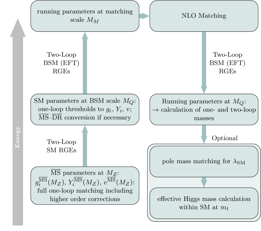
Figure 5: Schematic procedure of the numerical evaluation of a parameter point with SPheno when using the analytical setup to calculate matching conditions and implement them in SPheno

.

3.4 Numerical Approach

The second option to generate a SPheno version for an effective model including the matching conditions to a UV theory is to set up a suitable SPheno.m for the EFT from the very beginning. This file must include the following information in addition to the standard information which is usually defined in the SPheno.m files, see Appendix C:

SPheno.m

⬇

1MatchingToModel= { $MODELNAME };

2MatchingScale= { $LIST_OF_PARAMETERS };

3

4IncludeParticlesInThresholds={ $LIST_OF_FIELDS };

5

6AssumptionsMatchingScale={ $LIST };

7BoundaryMatchingScaleUp={ $LIST };

8BoundaryMatchingScaleDown={ $LIST };

9

10ParametersToSolveTadpoleMatchingScale={ $LIST_OF_PARAMETERS};

Note, this ansatz is not restricted to a single matching scale. Therefore, all entries are arrays of the dimension of the number of matching scales. The purpose of the different entries is

1. MatchingToModel is used to define the UV model(s), i.e. the model directory in SARAH.

2. IncludeParticlesInThresholds defines the list of particles which are included in the loop calculations.

3. AssumptionsMatchingScale is used to define simplifying assumptions at the matching scale. A common choice is to neglect the contributions from EW VEVs or other small parameters.

4. BoundaryMatchingScaleUp defines the boundary conditions to relate the parameters of the UV theory to the running parameters of the EFT when the RGEs run from low to high scales.

5. BoundaryMatchingScaleDown defines the boundary conditions to relate the parameters of the UV theory to the running parameters of the EFT when the RGEs run from high to low scales.

6. ParametersToSolveTadpoleMatchingScale defines the parameters that are fixed by the tadpole equations in the full theory.

Also one-loop matching conditions for fermionic interactions are available in the numerical approach. The full one-loop coupling is also indicated by using EFTcoupNLO, i.e.

⬇

1EFTcoupNLO[F1.F2.S][PL]

2EFTcoupNLO[F1.F2.S][PR]

where F1 and F2 are the involved fermions and S is the involved scalar. Yukawa-like interactions are chiral couplings. Therefore, the main difference to purely scalar couplings is the second argument containing PL/PR (for $P_{L,R}=\frac{1}{2}(1\pm\gamma_{5})$) to define which part of the coupling is meant. Moreover, the keyword ShiftCoupNLO can be used just to obtain the one-loop shift to a coupling, e.g.

⬇

1ShiftCoupNLO[F1.F2.S][PL]

2ShiftCoupNLO[F1.F2.S][PR]

Several examples for the usage of these options are given below.

3.4.1 One Matching Scale Without RGE Running Above

We start again with the simplest example of high-scale SUSY without any RGE running above the matching scale. Thus, the produced SPheno code will generate the same results as the one with the analytical approach in the last section. In order to set up a high-scale SUSY version with degenerate SUSY masses at the matching scale, the corresponding lines in the SPheno.m located in the model directory of the EFT, i.e. Models/HighScaleSUSY/MSSM/SPheno.m, must read

SPheno.m

⬇

1MatchingToModel= {"MSSM"};

2MatchingScale = {m0};

3

4UseParameterAsGUTscale = {m0};

5

6IncludeParticlesInThresholds={

7 {hh,Ah,Hpm,Su,Sd,Se,Sv,Chi,Cha}

8};

9

10AssumptionsHighScale={

11 {

12 {vd,epsUV*Cos[ArcTan[TanBeta]]},

13 {vu,epsUV*Sin[ArcTan[TanBeta]]}

14 }

15};

16

17BoundaryMatchingScaleUp={

18{

19 {Yu, Sqrt[1+TanBeta^2]/TanBeta*Yu},

20 {Yd, Sqrt[1+TanBeta^2]*Yd},

21 {Ye, Sqrt[1+TanBeta^2]*Ye}

22 }

23};

24

25BoundaryMatchingScaleDown={

26{

27 {\[Lambda], -1/3 EFTcoupNLO[hh[1].hh[1].hh[1].hh[1]]}

28 }

29};

30

31ParametersToSolveTadpoleMatchingScale={

32 {mHd2,mHu2}

33};

Note that for simple high-scale theories, without additional light fields, the SPheno.m could also be stored in the SM model directory as the two models are technically the same. The newly introduced models are described in Sec. 3.5.

The definitions are very similar to the analytical approach: the symbol epsUV again has been used to neglect specific parameters at the matching scale. An important difference is that we have not singled out the contributions from only third generation Yukawas because this would not give any performance improvement for the numerical calculation. Note, that it is also not necessary to define the matching for the Yukawas when running down. Moreover, we have used the option to define the scale where the RGE running should stop as function of an input parameter (UseParameterAsGUTscale = {m0}). Thus, SPheno will run the RGEs only to that scale and evaluate the SUSY boundary conditions.

The process to generate the SPheno output and to compile the Fortran code is identical to the final steps for the analytical approach:

1. Run MakeSPheno of SARAH with the new input file

   ⬇

   In[1]Start["HighScaleSUSY/MSSM"]

   In[2]MakeSPheno[]

2. Copy the files and compile SPheno

   ⬇

   1 > cp -r $SARAH_Directory/Output/SM/EWSB/SPheno $SPheno_Directory/HighScaleSUSY/

   2 > cd $SPheno_Directory

   3 > make Model=HighScaleSUSY

For a SPheno version generated in that way, two additional flags are available in the Les Houches input file to have some control over the calculations:

LesHouches.in

⬇

1Block SPhenoInput # SPheno specific input

2 201 1 # Turn on/off one-loop contributions in the matching

3 202 0 # Turn on/off contributions from off-diagonal wave-function renormalisation

Thus, these flags can be used to:

1. Turn on/off all one-loop contributions to the matching. By default, they are turned on. This might be helpful to check the size and importance of the one-loop corrections.

2. Turn on/off the contributions from the off-diagonal wave-function renormalisation. By default, they are turned off. See Sec. 2.2 for more details.

3.4.2 Running Above the Matching Scale

We can modify the last example easily to include also the running above the matching scale. This might be for instance necessary if one wants to apply the SUSY boundary conditions at the scale where the gauge couplings do unify but not at the matching scale. In order to do so, one needs to remove UseParameterAsGUTscale = {m0} from the last example and put instead

SPheno.m.GUT

⬇

4ConditionGUTscale = g1 == g2;

Thus, SPheno stops the running once the condition $g_{1}(Q)=g_{2}(Q)$ is fulfilled.
In addition, the matching conditions for the Yukawas are changed to

SPheno.m.GUT

⬇

17BoundaryMatchingScaleUp={

18 {

19 {Yu, Sqrt[1+TanBeta^2]/TanBeta*Yu - Sqrt[2]*ShiftCoupNLO[bar[Fu].Fu.hh[1]][PL]/ZH[1,2]},

20 {Yd, Sqrt[1+TanBeta^2]*Yd - Sqrt[2]*ShiftCoupNLO[bar[Fd].Fd.hh[1]][PL]/ZH[1,1]},

21 {Ye, Sqrt[1+TanBeta^2]*Ye - Sqrt[2]*ShiftCoupNLO[bar[Fe].Fe.hh[1]][PL]/ZH[1,1]}

22 }

23};

The need for the normalization onto the tree-level rotation matrix elements ZH is described in the next section. In that way, we can include the one-loop shifts to all Yukawa couplings which are necessary to have a consistent RGE running with two-loop SUSY RGEs between the matching and GUT scale, see also the discussion in Sec. 2.4. Note, we did not consider any generation indices for the involved fermions, i.e. the result of ShiftCoupNLO is a $3\times 3$ matrix. If one wants to safe program run-time it is possible to consider the one-loop shifts to the top Yukawa couplings only.

SPheno.m.GUT

⬇

18{…,

19 {Yu, Sqrt[1+TanBeta^2]/TanBeta*Yu},

20 {Yu[3,3], Yu[3,3] - Sqrt[2]*ShiftCoupNLO[bar[Fu[3]].Fu[3].hh[1]][PL]/ZH[1,2]},

21 …

22}

Moreover, the shifts for the gauge couplings are applied automatically.

3.4.3 Several Matching Scales

With the above settings one can now implement an arbitrary number of matching scales. However, as we have noted already in Sec. 3.3.3, the pole-mass matching to the SM is automatically included in the SPheno output. Thus, if a second matching scale, which is not too far away from the EW scale, is needed, one can simply rely on that. However, if more than two matching scales are needed, or if the matching to the SM should take place at such a high scale where the pole-mass matching might suffer from numerical problems, one can now start to build up towers of EFTs by defining more matching scales in SPheno.m. For instance, the full input to define the tower

SM  $\to$  THDM  $\to$  THDM + electroweakinos  $\to$  MSSM

is given in Appendix D. In this example we also make use of the functionality to calculate new fermionic couplings at the one-loop level below a matching scale:

SPheno.m

⬇

142BoundaryMatchingScaleDown={

143…

144 {g1u,-2*(EFTcoupNLO[Chi[fB].Chi[FHu0].hh[2]][PL])},

145 {g2u,2*(EFTcoupNLO[Chi[fW0].Chi[FHu0].hh[2]][PL])},

146 {g1d,2*(EFTcoupNLO[Chi[fB].Chi[FHd0].hh[1]][PL])},

147 {g2d,-2*(EFTcoupNLO[Chi[fW0].Chi[FHd0].hh[1]][PL])},

148…

149}

Here, $g_{1,2}^{u,d}$ are the split-SUSY couplings between the Higgs boson and a Higgsino-Gaugino pair, see e.g. Ref. Bagnaschi:2014rsa . We include these corrections by considering the one-loop amplitude between the Higgs boson and a pair of neutralinos. In this example we have also used another feature: we have not explicitly defined the generation indices of the involved neutralinos. The reason for this is: even if the neutralino mass matrix contains only zero’s under the given approximations ($\mu,M_{i}\ll M_{\rm SUSY}$), it is not clear how the mass eigenstates are ordered in the numerical run. Therefore, we have used the name of the gauge eigenstates. By doing that, SPheno checks during the numerical evaluation which of the mass eigenstates has the biggest contribution of the given gauge eigenstate. Of course, if the rotation matrix for the neutralinos is not equivalent to the unit matrix, i.e. if some mixing appears for instance because of effects of non-vanishing $\mu$, one needs to define

SPheno.m

⬇

142BoundaryMatchingScaleDown={

143…

144 {g1u,-2*(EFTcoupNLO[Chi[fB].Chi[FHu0].hh[2]][PL]/(ZN[fB,1]*ZN[FHu0,4]))},

145 …

146…

147}

Thus, the rotation to mass eigenstates, which should take place just at the weak scale, is divided out.

3.4.4 Summary

A summary of the numerical evaluation of a parameter point with SPheno which includes several matching scales $M_{M_{n}}$ and optionally also the running to the GUT scale $M_{G}$ is given in Fig. 6.

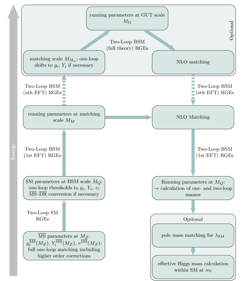
Figure 6: Schematic procedure of the numerical evaluation of a parameter point with SPheno when using the numerical setup to calculate matching conditions and implement them in SPheno.

3.5 Included Models and Input Files in SARAH

Several models which make use of the new functionality have already been implemented and are part of the publicly available SARAH version. All hierarchies considered for the MSSM so far are summarised in Fig. 7. Also for the NMSSM with very heavy particles two models exist: the high-scale NMSSM, where all SUSY fields are integrated out and a split-NMSSM, where the singlet and the SUSY fermions are kept.

Figure 7: Hierarchies for the MSSM so far included in SARAH. For the NMSSM versions similar to (a) and (c) exist as well. The zigzag line represent a large energy gap which is bridged with two-loop RGEs. The fields of the different mass symbols are explained in Sec. 4.

The names of the new models that make use of the numerical approach are listed in Tab. 1. Also for the analytical approach several input files are now included in SARAH. Those are summarised in Tab. 2. Based on these examples and by the explanations in this section, it is now straight-forward for the users to implement their own scenarios.

Model Name	EFT	UV model(s)	hierarchy
HighScaleSUSY/MSSM	SM	MSSM	(a)
HighScaleSUSY/NMSSM	SM	NMSSM	(a)
HighScaleSUSY/MSSMlowMA	THDM	MSSM	(b)
SplitSUSY/MSSM	SM+EWkinos	MSSM	(c)
SplitSUSY/NMSSM	SM+singlet+EWkinos	SMSSM	$\sim$(c)
SplitSUSY/MSSMlowMA	THDM+EWkinos	MSSM	(d)
SplitSUSY/MSSM_2scale	SM	MSSM $\to$ SM+EWkinos	(e)
SplitSUSY/MSSM_3scale	SM	MSSM $\to$ THDM+EWkinos $\to$ THDM	(f)

Table 1: The names of the new models which are part of SARAH 4.14.0. The hierarchy in the last column refers to Fig. 7. For the split-NMSSM also a light singlet is present, i.e. the hierarchy is similar to $(c)$, but not identical.

File Name	EFT	UV model	hierarchy
MSSM/Matching_HighScaleSUSY.m	SM	MSSM	(a)
NMSSM/Matching_HighScaleSUSY.m	SM	NMSSM	(a)
MSSM/Matching_SplitSUSY.m	SM+EWkinos	NMSSM	$\sim$(c)
MSSM/Matching_THDM.m	THDM	MSSM	(b)
SMSSM/Matching_SplitSUSY.m	SM+singlet+EWkinos	SMSSM	(c)

Table 2: Input files for the analytical approach which are now delivered with SARAH. The hierarchy in the last column refers to Fig. 7. For the split-NMSSM also a light singlet is present, i.e. the hierarchy is similar to $(c)$, but not identical.

4 Examples, Self-Consistency Checks and Comparisons with Other Codes

The following section describes realistic examples of practical applications of the presented framework. We consider different high-scale SUSY scenarios which were already studied intensively in literature. In particular comparisons between predictions for the SM Higgs boson mass derived with our generic setup against dedicated tools and calculations are made. In this context, we demonstrate also the perfect agreement between the two available options to use SARAH/SPheno for numerical studies. Finally, we also show that one can easily obtain precise results for other high-scale extensions for which no other tool existed so far.

4.1 Low-Energy Limits of the MSSM

In the introduction it was already mentioned that SUSY models with a SUSY breaking scale well above the electroweak scale became more popular in the recent years. While in these scenarios the direct observation of SUSY states is difficult or even impossible, these models are severely constrained by the Higgs boson mass measurements. For instance, if the masses of all superpartners are degenerate, the highest possible SUSY breaking scale in the MSSM is about $10^{10}$ GeV Bagnaschi:2014rsa . For higher scales, the predicted $m_{h}$ always becomes too large. Since the Higgs boson mass in these models is the crucial observable, a precise calculation is mandatory and specialised codes have been developed to get reliable predictions. We are going to consider three different cases: (i) split-SUSY in which all SUSY scalars are very heavy, but electroweakinos might stay moderately light, (ii) high-scale SUSY in which all SUSY masses and the additional Higgs boson masses are large and degenerate, (iii) high-scale SUSY with a second light(ish) Higgs doublet. In all three cases we work with the following reduced set of input parameters

$$m_{0},\,M_{\chi},\,M_{A},\,A_{0}\,\,\,\text{and}\,\,\,\tan\beta\,,$$ (30)

with

$$m_{\tilde{u}}^{2}=m_{\tilde{d}}^{2}=m_{\tilde{q}}^{2}=m_{\tilde{l}}^{2}=m_{\tilde{e}}^{2}\equiv{\bf 1}m_{0}^{2}\,,$$ (31)

$$M_{1}=M_{2}=M_{3}=\mu\equiv M_{\chi}\,,$$ (32)

$$B_{\mu}\equiv M_{A}^{2}\frac{\tan\beta}{1+\tan^{2}\beta}\,,$$ (33)

$$T_{i}\equiv A_{0}Y_{i}\hskip 17.07182pt\text{and}\hskip 17.07182pti=\{e,d,u\}\,.$$ (34)

Here, $m^{2}_{\tilde{f}}$ are the soft masses squared for all chiral superfields, $M_{A}$ is the mass of the heavy Higgs doublet, $M_{i}$ are the soft gaugino masses, $\mu$ is the Higgsino mass term in the superpotential, and $B_{\mu}$, $T_{i}$ are the soft-breaking equivalents of the $\mu$-term and the Yukawa couplings in the superpotential.

4.1.1 Split-SUSY: MSSM $\to$ SM & Electroweakinos & Gluinos

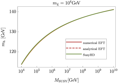
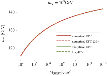
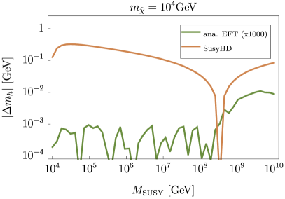
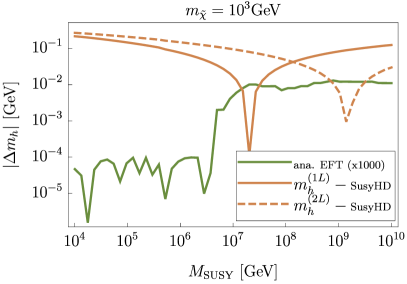
Figure 8: Prediction for the SM Higgs boson mass $m_{h}$ in split-SUSY as function of $M_{\rm SUSY}$, which is the mass scale of all SUSY scalars, and for two different values of $M_{\chi}$, which is the mass scale of all SUSY fermions. In addition, we used here $\tan\beta=3$. The blue and purple lines show the results of SPheno using the analytical or numerical approach to obtain the matching conditions at $M_{\rm SUSY}$, while the green line corresponds to the results of SusyHD. For SPheno and $M_{\chi}=1$ TeV, we show also the result when turning on the two-loop corrections at the low scale. The first row shows the calculated values for $m_{h}$, while the second give the differences between the calculations compared to the numerical approach.

Split-SUSY with very heavy SUSY scalars but significantly lighter SUSY fermions keeps most of the nice SUSY properties like gauge coupling unification and provides a viable dark matter candidate. In this setup, the full MSSM is matched to the SM extended by additional fermions. The Lagrangian of the effective theory reads

$$\mathcal{L}_{\rm EFT}= \mathcal{L}_{\rm SM}-\left(\frac{1}{2}M_{3}\tilde{g}^{\alpha}\tilde{g}^{\alpha}+\frac{1}{2}M_{2}\tilde{W}^{a}\tilde{W}^{a}+\frac{1}{2}M_{B}\tilde{B}\tilde{B}+\mu\tilde{H}_{u}^{T}\epsilon\tilde{H}_{d}\,+\,\text{h.c.}\right)$$

$$-\left[\frac{1}{\sqrt{2}}H^{\dagger}\left(\tilde{g}_{2u}\sigma^{a}\tilde{W}^{a}+\tilde{g}_{1u}\tilde{B}\right)\tilde{H}_{u}+\frac{1}{\sqrt{2}}H^{T}\epsilon\left(-\tilde{g}_{2d}\sigma^{a}\tilde{W}^{a}+\tilde{g}_{1d}\tilde{B}\right)\tilde{H}_{d}\,+\,\text{h.c.}\right]\,,$$ (35)

where the Yukawa couplings $g_{1,2}^{u,d}$ are as in the example of Sec. 3.4.3, $\sigma^{a}$ are the pauli matrices and $\alpha=1,...,8$. In order to calculate the Higgs boson mass in this model, the common approach is to (i) decouple the SUSY scalars at the scale $M_{\rm SUSY}$ and calculate $\lambda_{SM}(M_{\rm SUSY})$ including important higher-order corrections, (ii) run the split-SUSY RGEs to the scale $M_{\chi}$ of the remaining SUSY states and calculate the shift in $\lambda_{SM}(M_{\chi})$, (iii) run the SM RGEs to $m_{t}$ and calculate $m_{h}(m_{t})$ at the two-loop level. The full results for the one-loop matching conditions at $M_{\rm SUSY}$ and $M_{\chi}$ were given in Ref. Bagnaschi:2014rsa . Also the dominant two-loop corrections to $\lambda_{SM}$ of order $O(\alpha_{t}^{2}\alpha_{s})$ have been included in this reference. These results were implemented into the code SusyHD Vega:2015fna and also FlexibleSUSY Athron:2014yba ; Athron:2017fvs uses the matching conditions from literature.

We have compared the analytical expressions of Ref. Bagnaschi:2014rsa for the one-loop thresholds with the results of SARAH and found perfect agreement. Thus, we can immediately go to the discussion of the comparison of the numerical results of SPheno and SusyHD. Even if the expressions for the thresholds agree, there are many other ingredients which enter the Higgs mass prediction. Most importantly, the determination of the top Yukawa coupling which affects all comparisons shown here. Also higher-order corrections for high-scale SUSY scenarios are implemented to some extent in other codes which are not (yet) available in our generic setup. The corresponding model in SARAH which we have set up for this scenario is

SplitSUSY/MSSM

We show in Fig. 8 the calculated Higgs boson mass by SusyHD and SPheno as function of $M_{\rm SUSY}$ for two different choices of $M_{\chi}$. First of all, one can see that the overall agreement is very good between all calculations: for the two calculations implemented in SARAH/SPheno we find agreement up to the numerical precision, while the biggest difference between SPheno and SusyHD is well below one GeV for all considered values of $M_{\rm SUSY}$.

For the case of electroweakino masses of 1 TeV we show also the SPheno result when using a two-loop fixed-order calculation in the EFT. We see, in agreement with a previous study in Ref. Braathen:2017izn , that the two-loop contributions of the additional fermions have only a mild effect on the SM-like Higgs boson mass.

4.1.2 High-scale SUSY: MSSM $\to$ SM

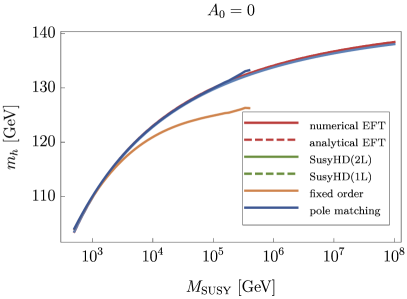
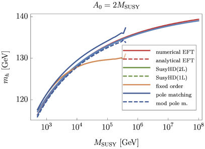
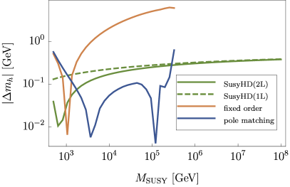
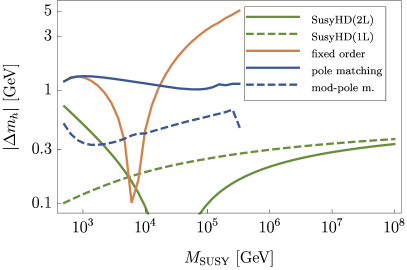
Figure 9: Comparison between SPheno and SusyHD for high-scale SUSY as function of the SUSY scale $M_{\rm SUSY}=m_{0}=M_{\chi}=M_{A}$. Here, we used $\tan\beta=10$ and two different values of $A_{0}$. For SPheno we give the results using the analytical and numerical approach to perform the matching at the SUSY scale. Also the results of a fixed-order calculation and using a pole-mass matching are included. For SusyHD the results with and without the two-loop corrections in the matching of $\lambda_{SM}$ are depicted. The first row shows the calculated Higgs boson mass of all codes, while the second row gives the differences between the different calculations w.r.t. the numerical approach.

An even more extreme setup than split-SUSY is high-scale SUSY in which all SUSY partners are very heavy. Thus, the effective model is just the SM, i.e.

$$\mathcal{L}_{\rm EFT}=\mathcal{L}_{\rm SM}\,,$$ (36)

and the only visible impact of SUSY is the prediction of $\lambda_{SM}$ at the matching scale $M_{\rm SUSY}\simeq M_{\chi}\simeq M_{A}$. The matching conditions at the SUSY scale are just the combination of the two matching conditions for split-SUSY applied at a single matching. Thus, it is obvious that also for this case a full agreement between our analytical results and those of Ref. Bagnaschi:2014rsa exists. However, Ref. Bagnaschi:2014rsa includes also the dominant two-loop corrections in the case of high-scale SUSY which also entered the code SusyHD. Therefore, it’s worth to discuss also the numerical differences between SPheno and SusyHD for the case of high-scale SUSY. The model implemenation in SARAH is called

HighScaleSUSY/MSSM

The results are summarised in Fig. 9. In addition to the comparison to SusyHD we also compare the results to two other calculations: a standard fixed-order calculation as well as an EFT calculation based on the pole-mass matching Staub:2017jnp . In the pole-mass matching, the quartic coupling $\lambda_{SM}$ is calculated from the condition

$$m_{h}^{2,\rm pole\ SM}(M_{\rm SUSY})\equiv m_{h}^{2,\rm pole\ MSSM}(M_{\rm SUSY})$$ (37)

which can be translated into

$$\lambda_{SM}(M_{\rm SUSY})=\frac{1}{v^{2}(M_{\rm SUSY})}\left(m_{h}^{2,\rm pole\ MSSM}(M_{\rm SUSY})-\Pi_{h}^{\rm SM}(M_{\rm SUSY})\right)\,,$$ (38)

where $\Pi^{\rm SM}_{h}$ are the loop corrections to $m_{h}$ known from the SM. The pole-mass matching has the advantage that also terms $\frac{v}{M_{\rm SUSY}}$ are included and that only two-point functions need to be calculated instead of four-point functions, see Ref. Athron:2016fuq for more details. On the other side, this approach has also some drawbacks. It is mainly restricted to the SM as EFT, but it is not straightforward to be used in models with several light scalars. Also a consistent matching at the two-loop level needs some fiddling with the running parameters which enter the different parts of Eq. 38, see Ref. Athron:2017fvs . While SPheno by default used $\overline{\text{MS}}$ parameters to calculate $\Pi_{h}^{\rm SM}$ and $\overline{\text{DR}}$ SUSY parameters in the calculation of $m_{h}^{2,\rm pole\ MSSM}(M_{\rm SUSY})$, we also give the results for using $Y_{t}^{\overline{\text{MS}}}$ in both calculations. This is called ’modified pole-mass matching’ in the left plot of Fig. 9. The difference between both results is a two-loop effect and could be taken as estimate of the remaining uncertainty in the one-loop pole-mass matching.

Moreover, we find that the pole-mass matching becomes also numerically unstable –at least in SPheno– once $M_{\rm SUSY}\gg v$ is used because the loop functions used for the pole-mass calculations are not optimised for these cases: we see in Fig. 9 that the pole-mass matching breaks down at $M_{\rm SUSY}\simeq 5\cdot 10^{5}$ GeV. Nevertheless, we find that the agreement between the pole-mass matching and the direct matching procedure presented here is very good for SUSY scales up to 100 TeV. One finds also that the fixed-order calculation agrees perfectly with the pole-mass matching for $M_{\rm SUSY}$ below 1 TeV. Of course, for larger SUSY scales, the discrepancy between the fixed-order calculation and all EFT calculations grows very rapidly.

We come back to the comparison with SusyHD: we see that the agreement between SPheno and SusyHD is also very good and the differences are always of the level of 1 GeV or below. The 1 GeV differences appear only for the choice $A_{0}=2M_{\rm SUSY}$ and $M_{\rm SUSY}$ around the TeV scale. In that case, the two-loop corrections missing in SPheno play some role. However, for larger $M_{\rm SUSY}$ or smaller trilinear terms, these two-loop corrections cause only a moderate shift – or become even completely negligible. Thus, we think that it is not a substantial drawback of our setup that ’only’ one-loop corrections are included so far.

4.1.3 High-scale SUSY with intermediate $M_{A}$: MSSM $\to$ THDM

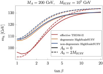
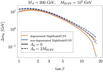
Figure 10: The Higgs boson mass prediction as function of $\tan\beta$ for a high-scale SUSY scenario with low $M_{A}$ and two different values of $A_{0}$. The blue lines show the results for a proper matching of the MSSM to the THDM-II. The green lines correspond to the matching of the MSSM to the SM where either all scalars, including the additional Higgs states, are assumed to be degenerate, or in which the actual value of $M_{A}$ has been used. The figure on the right show the difference between the matching to the THDM and to the SM.

In the last example we have assumed that all BSM particles are very heavy and degenerate. An important deviation of this ansatz is the possibility that the second Higgs doublet remains light, i.e. only fields with negative $R$-parity are very heavy. In this case, the low-energy theory of the MSSM is a Two-Higgs-Doublet-Model type-II. The Lagrangian of the EFT is

$$-\mathcal{L}_{\rm EFT}= m_{1}^{2}|H_{1}|^{2}+m_{2}^{2}|H_{2}|^{2}+\lambda_{1}|H_{1}|^{4}+\lambda_{2}|H_{2}|^{4}+\lambda_{3}|H_{1}|^{2}|H_{2}|^{2}+\lambda_{4}|H_{2}^{\dagger}H_{1}|^{2}$$

$$+\left(m_{12}H_{1}^{\dagger}H_{2}+\frac{1}{2}\lambda_{5}(H_{2}^{\dagger}H_{1})^{2}+\lambda_{6}|H_{1}|^{2}H_{1}^{\dagger}H_{2}+\lambda_{7}|H_{2}|^{2}H_{1}^{\dagger}H_{2}+\text{c.c.}\right)$$

$$+\left(Y_{d}H_{1}^{\dagger}\bar{d}q+Y_{e}H_{1}^{\dagger}\bar{e}l-Y_{u}H_{2}\bar{u}q+\text{h.c.}\right)\,.$$ (39)

One can make the following association between fields at the SUSY scale to calculate the matching conditions

$$H_{1}\equiv-i\sigma_{2}H_{d}^{*}\quad\text{and}\quad H_{2}\equiv H_{u}\,.$$ (40)

However, this choice is not unique as there is no preferred basis of Higgs doublets in a general THDM, i.e. one could also interchange $H_{1}$ and $H_{2}$ or take any linear combination of them. With the common choice made in Eq. 40, one can simultaneously apply a rotation into the mass basis on ($H_{1},H_{2}$) and ($H_{u}$,$-i\sigma_{2}H_{d}^{*}$) so that the tree-level mixing angle $\tan\beta$ of the MSSM coincides with the effective THDM.

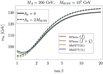
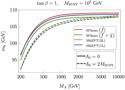
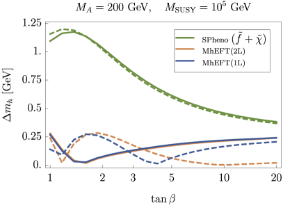
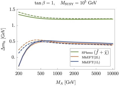
Figure 11: Comparison between MhEFT and SPheno for a variation of $\tan\beta$ (left) or $M_{A}$ (right). All SUSY masses are assumed to be degenerate and identical to $M_{\rm SUSY}$, and the results for two different values of $A_{0}$ are shown.

The dominant threshold corrections to $\lambda_{1}$ – $\lambda_{7}$ involving third generation Yukawa couplings are available in literature Haber:1990aw . We have double checked the analytical expressions derived by SARAH and found full agreement.

The importance of the proper matching to the THDM for the case $M_{A}\ll M_{\rm SUSY}$ has been pointed out in Ref. Lee:2015uza . It was found that in particular for small $\tan\beta$ very large difference to a one-scale matching appear. In order to demonstrate that, we compare in Fig. 10 the Higgs boson mass prediction using the proper matching of the MSSM to the THDM against the simplified ansatz of decoupling the second Higgs doublet together with all other BSM states at $M_{\rm SUSY}$. First of all, one can check that the results for the matching to the SM change only moderately when using the actual value of $M_{A}$ in the one-scale matching compared to the fully degenerate case $M_{A}=m_{0}=M_{\rm SUSY}$. This only causes a shift of at most $\sim$1 GeV for $\tan\beta=1$. On the other side, there are big difference showing up when performing the matching to the THDM. For values of $\tan\beta$ close to 1, the discrepancy can be as large as 10 GeV, while it rapidly decreases with increasing $\tan\beta$. For $\tan\beta=10$, the differences between both matching approaches are about 1 GeV.

Since we have demonstrated the importance of performing the matching to the THDM properly for the case of a light second Higgs doublet, it is clear that codes were developed to include these effects. The first tool in this direction was MhEFT which uses a purely EFT ansatz Lee:2015uza . In a recent update of FeynHiggs a hybrid ansatz combining the fixed-order calculation with higher-order terms was implemented Bahl:2018jom .The overall agreement between both codes turned out to be good once a careful translation between the parameters in both renormalisation schemes was done. Since MhEFT is much closer to the ansatz of SARAH/SPheno we are going to compare our results with this tool. For this purpose, we have set up the model

HighScaleSUSY/MSSMlowMA

in SARAH. We show in Fig. 11 the results of MhEFT and SPheno when varying $\tan\beta$ or $M_{A}$ for a fixed SUSY scale of 100 TeV. The agreement between both codes is always good. The maximal difference for comparable calculations is about 0.5 GeV and can be even smaller for $M_{A}$ below 500 GeV and arbitrary values of $\tan\beta$. The differences are due to the three-loop RGEs which are included in MhEFT in the running between $m_{t}$ and $M_{A}$ while SPheno uses always two-loop RGEs. This explains the flattening of the difference as the top quark Yukawa coupling runs fastest near the weak scale. One can also see that the impact of the additional two-loop corrections implemented in MhEFT is very moderate. Thus the main source of the difference is the determination of the running top Yukawa coupling. In contrast, the additional one-loop corrections due to gauginos, which were presented very recently also in Ref. Bahl:2018jom , can be easily included in SPheno using the numerical matching interface. For the considered choice of parameters these have numerically a bigger effect than the two-loop corrections and cause a shift of 1–1.5 GeV.

4.2 High-scale NMSSM

Up to now we have only discussed examples of models involving very heavy BSM particles which could already be studied with public tools like SusyHD, MhEFT, FlexibleSUSY or FeynHiggs. These are just different low-energy limits of the MSSM. However, our framework is not restricted to this case and in principle any SUSY or non-SUSY model could be considered as high-scale theory. We show that crucial differences compared to the MSSM show already up in the case of the NMSSM. The NMSSM involves an additional gauge singlet superfield $\hat{S}$ which leads to the following superpotential after imposing a $Z_{3}$ symmetry to forbid all dimensionful parameters

$$W_{\rm NMSSM}=\lambda_{S}\hat{S}\hat{H}_{d}\hat{H}_{u}+\frac{1}{3}\kappa\hat{S}^{3}+W_{Y}\,,$$ (41)

where $W_{Y}$ represents the terms involving Yukawa couplings that are identical to the MSSM. The NMSSM-specific soft-SUSY breaking parameters are

$$-\mathcal{L}_{\rm SB,\ NMSSM}=m_{S}^{2}|S|^{2}+(T_{\lambda}SH_{d}H_{u}+\frac{1}{3}T_{\kappa}S^{3}+c.c.)\,.$$ (42)

The scalar singlet $S$ can receive a VEV even without EWSB

$$\langle S\rangle=\frac{1}{\sqrt{2}}v_{S}$$ (43)

which causes an effective Higgsino mass term

$$\mu_{\rm eff}=\frac{1}{\sqrt{2}}\lambda_{S}v_{S}\,.$$ (44)

We can now study what the impact of the additional gauge singlet in a high-scale SUSY scenario is. For this purpose, we impose the following relation among the parameters

$$\kappa= \frac{1}{2}\lambda_{S}$$ (45)

$$\mu_{\rm eff}= m_{0}$$ (46)

$$T_{\kappa}= -\frac{1}{3}\lambda_{S}m_{0}$$ (47)

$$T_{\lambda}= \frac{1}{2}\lambda_{S}m_{0}\left(\sin(2\beta)-1\right)\,.$$ (48)

This leads to a nearly degenerate spectrum of SUSY fields with masses of $m_{0}$ apart from one CP-even singlet which has a mass of $\sqrt{\frac{2}{3}}m_{0}$. Thus, the EFT model is again the SM, i.e.

$$\mathcal{L}_{\rm EFT}=\mathcal{L}_{\rm SM}$$ (49)

The full high-scale model has three free parameters

$$m_{0},\quad\lambda_{S},\quad\tan\beta\,.$$ (50)

The MSSM limit is obtained for $\lambda_{S}\to 0$. We have implemented this model in SARAH as

HighScaleSUSY/NMSSM

The predicted mass for the SM-like Higgs boson as function of the SUSY scale $M_{\rm SUSY}$ is shown in Fig. 12 for different values of $\lambda_{S}$. Thus, one can see that there are significant shifts in the Higgs boson mass already for values of $\lambda_{S}$ of 0.2 or 0.3. In general, one finds that the Higgs boson mass decreases with increasing $\lambda_{S}$. The main reason for this are tree-level contributions proportional to $\frac{T_{\lambda}^{2}}{m_{S}^{2}}\simeq\frac{1}{4}\lambda_{S}^{2}$ which dominate for small $\tan\beta$ over the D-term contributions. Thus, the conclusion that the maximal possible SUSY scale in agreement with $m_{h}$ is about $10^{10}$ GeV only holds for the MSSM, while in the NMSSM one can push $M_{\rm SUSY}$ towards the Planck scale without being in conflict with Higgs boson mass measurements.

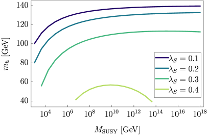
Figure 12: The Higgs boson mass in a high-scale SUSY scenario based on the NMSSM with fixed $\tan\beta=4$. All SUSY fields including the singlets are (nearly) degenerate with a mass of $M_{\rm SUSY}$. The given values of $\lambda_{S}$ determine the coupling strength of the gauge singlet and the two Higgs doublets in the NMSSM at the matching scale.

Of course, one could now start to consider also other low-energy limits of the NMSSM. However, this is beyond the scope of this paper here and interesting applications are given elsewhere SplitNMSSM .

5 Summary

We have presented an extension of the Mathematica package SARAH which derives the one-loop matching conditions for effective scalar couplings based on a UV theory. Two different approaches exists, which are based on either an analytical or fully numerical calculation. The full agreement between both calculations and analytical results available in literature has been pointed out. Furthermore, good agreement with specialised codes to study Split- or High-scale SUSY like SusyHD or MhEFT was shown. Since our approach is completely general, it can be used to study UV completions of a large variety of BSM models with and without an extended Higgs sector.

Appendix A Generic Diagrams

In this appendix we provide a complete list of all possible one-loop diagrams with 2, 3 and 4 external scalars and internal fermions or scalars. The results were obtained in the limit of vanishing external momenta using the computer programs FeynArts and FormCalc Hahn:2000kx ; Hahn:2009bf .

We distinguish between topologies, where neither the statistical nature (spin=0,1,$\nicefrac{{1}}{{2}}$) nor the mass (light or heavy i.e. zero or non-zero) of internal fields is specified and generic diagrams, where the spin of all fields is specified but not their mass hierarchies. This is still a model-independent graph but gives the possibility to write down a model-independent generic amplitude. Couplings and masses appearing in the expression of a generic amplitude are seen as generic couplings that do not have any relation to parameters used in other generic amplitudes.

As already mentioned in Sec. 3, SARAH’s analytical matching interface does not only compute the full one-loop contribution but is also able to compute a subset of diagrams based on e.g. a choice of topologies. For this reason, a notation with a successive structure is introduced. A topology is described by a string consisting of maximum four characters. It starts with the specification of the diagram type which can be tree-level (T), self-energy (S), WFR (W) or ordinary one-loop diagram (blank) followed by a letter specifying the type of the involved loop integral defined in Appendix B. In the next digit, the number of external fields is specified. If the diagram contains an internal single propagator additional to a loop (2) or a loop only (1) is denoted by the next digit (blank means that no diagrams with additional internal lines exist). The last digit is a counting index (blank means only one diagram of that type exists). An example explanation of the notation is given in Fig. 13. The Topologies options of the matching routines can either select certain topologies, like {B[4][2][1],B[4][2][2]} , or successively select topology groups, like {B[4][2]} or just {B[4]}. All possible topologies and groups are stored in the list TopoNotation. In the following, we list the analytical expressions for all generic amplitudes as well as the topologies they belong to in the format used in the SARAH matching routines.

(a)

(b) B[4][2][1]

Figure 13: Notation on topologies appearing in generic one-loop diagrams. The example expression explained in (a) corresponds for instance to the diagram shown in (b).

A.1 Tree-Level Contributions

A.1.1 Quartic Couplings

There are two tree-level topologies with four external scalars. The first one is a local quartic coupling which could for example be given by supersymmetric D-terms and/or F-terms while the second one has one internal propagator, necessarily heavy and of bosonic nature. Thus, fermions can only enter one-loop and higher-order corrections.

$${\displaystyle\text{\leavevmode\lstinline{{\lst@@@set@language\lst@@@set@numbers\lst@@@set@frame\lst@@@set@rulecolor\lst@@@set@numbers\small{\@listingGroup{ltx_lst_identifier}{T}}[4][1]}}}}\equiv\begin{aligned} \includegraphics{FeynMF/FM_Tree1}\end{aligned} \mathcal{M}=c$$ (51)

$${\displaystyle\text{\leavevmode\lstinline{{\lst@@@set@language\lst@@@set@numbers\lst@@@set@frame\lst@@@set@rulecolor\lst@@@set@numbers\small{\@listingGroup{ltx_lst_identifier}{T}}[4][2]}}}}\equiv\begin{aligned} \includegraphics{FeynMF/FM_Tree2}\end{aligned} \mathcal{M}=-\frac{c_{1}c_{2}}{m_{1}^{2}}$$ (52)

A.1.2 Cubic Couplings

Since there is only one three-point topology, the matching of trilinear couplings at tree level is trivial.

$${\displaystyle\text{\leavevmode\lstinline{{\lst@@@set@language\lst@@@set@numbers\lst@@@set@frame\lst@@@set@rulecolor\lst@@@set@numbers\small{\@listingGroup{ltx_lst_identifier}{T}}[3]}}}}\equiv\begin{aligned} \includegraphics{FeynMF/FM_TreeC}\end{aligned} \mathcal{M}=c$$ (53)

A.1.3 Bilinear Parameters

The two-point function is necessary for the matching of scalar sectors that involve non-Higgs scalar fields i.e. scalars that do not develop a VEV. In this case the scalar masses and couplings are independent parameters and have to be matched separately.

$${\displaystyle\text{\leavevmode\lstinline{{\lst@@@set@language\lst@@@set@numbers\lst@@@set@frame\lst@@@set@rulecolor\lst@@@set@numbers\small{\@listingGroup{ltx_lst_identifier}{T}}[2]}}}}\equiv\begin{aligned} \includegraphics{FeynMF/FM_TreeBi}\end{aligned} \mathcal{M}=m^{2}$$ (54)

A.2 One-Loop Contributions

At the one-loop order, we distinguish between irreducible diagrams and reducible diagrams which contain an additional internal propagator line.

A.2.1 Irreducible Diagrams

Quartic Couplings

Since we consider renormalisable theories, fermions can only enter the one-loop corrections to quartic couplings in box diagrams (topology D, note that D[4] is not a valid topology as it is a reserved Mathematica symbol). The generic diagrams and amplitudes are

$${\displaystyle\text{\leavevmode\lstinline{{\lst@@@set@language\lst@@@set@numbers\lst@@@set@frame\lst@@@set@rulecolor\lst@@@set@numbers\small{\@listingGroup{ltx_lst_identifier}{B}}[4][1]}}}}\equiv\begin{aligned} \includegraphics{FeynMF/FM_B}\end{aligned} \mathcal{M}=\frac{1}{2}c_{1}c_{2}\overline{B}_{0}(m_{1}^{2},m_{2}^{2})$$ (55)

$${\displaystyle\text{\leavevmode\lstinline{{\lst@@@set@language\lst@@@set@numbers\lst@@@set@frame\lst@@@set@rulecolor\lst@@@set@numbers\small{\@listingGroup{ltx_lst_identifier}{C}}[4][1]}}}}\equiv\begin{aligned} \includegraphics{FeynMF/FM_Triangle}\end{aligned} \mathcal{M}=-c_{1}c_{2}c_{3}\overline{C}_{0}(m_{1}^{2},m_{2}^{2},m_{3}^{2})$$ (56)

$${\displaystyle\text{\leavevmode\lstinline{{\lst@@@set@language\lst@@@set@numbers\lst@@@set@frame\lst@@@set@rulecolor\lst@@@set@numbers\small{\@listingGroup{ltx_lst_identifier}{D}}}}}}\equiv\begin{aligned} \includegraphics{FeynMF/FM_BoxS}\end{aligned} \mathcal{M}=c_{1}c_{2}c_{3}c_{4}\overline{D}_{0}(m_{1}^{2},m_{2}^{2},m_{3}^{2},m_{4}^{2})$$ (57)

$${\displaystyle\text{\leavevmode\lstinline{{\lst@@@set@language\lst@@@set@numbers\lst@@@set@frame\lst@@@set@rulecolor\lst@@@set@numbers\small{\@listingGroup{ltx_lst_identifier}{D}}}}}}\equiv\begin{aligned} \includegraphics{FeynMF/FM_BoxF}\end{aligned} \mathcal{M}=\mathcal{M}_{F}^{4}$$ (58)

with

$$\mathcal{M}_{F}^{4}= \left(c_{1}^{R}c_{2}^{L}c_{3}^{R}c_{4}^{L}+c_{1}^{L}c_{2}^{R}c_{3}^{L}c_{4}^{R}\right)\overline{B}_{0}(m_{3}^{2},m_{4}^{2})+\Big{[}(c_{1}^{R}c_{2}^{L}c_{3}^{R}c_{4}^{L}+c_{1}^{L}c_{2}^{R}c_{3}^{L}c_{4}^{R})(m_{1}^{2}+m_{2}^{2})$$

$$+c_{4}^{L}(c_{1}^{L}m_{1}(c_{2}^{L}c_{3}^{R}m_{2}+c_{2}^{R}c_{3}^{R}m_{3}+c_{2}^{R}c_{3}^{L}m_{4})+c_{1}^{R}(c_{2}^{L}c_{3}^{L}m_{3}m_{4}+c_{2}^{R}m_{2}(c_{3}^{R}m_{3}+c_{3}^{L}m_{4})))+$$

$$c_{4}^{R}(c_{1}^{R}m_{1}(c_{2}^{R}c_{3}^{L}m_{2}+c_{2}^{L}c_{3}^{L}m_{3}+c_{2}^{L}c_{3}^{R}m_{4})+c_{1}^{L}(c_{2}^{R}c_{3}^{R}m_{3}m_{4}+c_{2}^{L}m_{2}(c_{3}^{L}m_{3}+c_{3}^{R}m_{4})))\Big{]}\overline{C}_{0}(m_{2}^{2},m_{3}^{2},m_{4}^{2})+$$

$$+ m_{1}\Big{[}c_{1}^{L}(c_{2}^{L}m_{2}(c_{3}^{L}m_{3}(c_{4}^{R}m_{1}+c_{4}^{L}m_{4})+c_{3}^{R}m_{1}(c_{4}^{L}m_{1}+c_{4}^{R}m_{4}))+c_{2}^{R}m_{1}(c_{3}^{L}m_{1}(c_{4}^{R}m_{1}+c_{4}^{L}m_{4})$$

$$+c_{3}^{R}m_{3}(c_{4}^{L}m_{1}+c_{4}^{R}m_{4})))+c_{1}^{R}(c_{2}^{L}m_{1}(c_{3}^{L}m_{3}(c_{4}^{R}m_{1}+c_{4}^{L}m_{4})+c_{3}^{R}m_{1}(c_{4}^{L}m_{1}+c_{4}^{R}m_{4}))$$

$$+c_{2}^{R}m_{2}(c_{3}^{L}m_{1}(c_{4}^{R}m_{1}+c_{4}^{L}m_{4})+c_{3}^{R}m_{3}(c_{4}^{L}m_{1}+c_{4}^{R}m_{4})))\Big{]}\overline{D}_{0}(m_{1}^{2},m_{2}^{2},m_{3}^{2},m_{4}^{2}\,,$$ (59)

where $c_{i}^{R,L}$ are the left- and right-handed fermion couplings corresponding to the vertices $c_{i}$ in (58).

Cubic Couplings

The effective trilinear couplings are

$${\displaystyle\text{\leavevmode\lstinline{{\lst@@@set@language\lst@@@set@numbers\lst@@@set@frame\lst@@@set@rulecolor\lst@@@set@numbers\small{\@listingGroup{ltx_lst_identifier}{B}}[3]}}}}\equiv\begin{aligned} \includegraphics{FeynMF/FM_Bcubic}\end{aligned} \mathcal{M}=\frac{1}{2}c_{1}c_{2}\overline{B}_{0}(m_{1}^{2},m_{2}^{2})$$ (60)

$${\displaystyle\text{\leavevmode\lstinline{{\lst@@@set@language\lst@@@set@numbers\lst@@@set@frame\lst@@@set@rulecolor\lst@@@set@numbers\small{\@listingGroup{ltx_lst_identifier}{C}}[3]}}}}\equiv\begin{aligned} \includegraphics{FeynMF/FM_TriangleC}\end{aligned} \mathcal{M}=-c_{1}c_{2}c_{3}\overline{C}_{0}(m_{1}^{2},m_{2}^{2},m_{3}^{2})$$ (61)

$${\displaystyle\text{\leavevmode\lstinline{{\lst@@@set@language\lst@@@set@numbers\lst@@@set@frame\lst@@@set@rulecolor\lst@@@set@numbers\small{\@listingGroup{ltx_lst_identifier}{C}}[3]}}}}\equiv\begin{aligned} \includegraphics{FeynMF/FM_TriangleCF}\end{aligned} \mathcal{M}=\mathcal{M}_{F}^{3}$$ (62)

with

$$\mathcal{M}_{3}^{F}= (-c_{1}^{R}(c_{2}^{L}c_{3}^{R}m_{1}+c_{2}^{R}c_{3}^{L}m_{2}+c_{2}^{L}c_{3}^{L}m_{3})-c_{1}^{L}(c_{2}^{R}c_{3}^{L}m_{1}+c_{2}^{L}c_{3}^{R}m_{2}+c_{2}^{R}c_{3}^{R}m_{3}))\overline{B}_{0}(m_{2}^{2},m_{3}^{2})$$

$$+\Big{[}-m_{1}(c_{1}^{L}(c_{2}^{L}m_{2}(c_{3}^{R}m_{1}+c_{3}^{L}m_{3})+c_{2}^{R}m_{1}(c_{3}^{L}m_{1}+c_{3}^{R}m_{3}))$$

$$\hskip 56.9055pt+c_{1}^{R}(c_{2}^{L}m_{1}(c_{3}^{R}m_{1}+c_{3}^{L}m_{3})+c_{2}^{R}m_{2}(c_{3}^{L}m_{1}+c_{3}^{R}m_{3})))\Big{]}\overline{C}_{0}(m_{1}^{2},m_{2}^{2},m_{3}^{2})\,.$$ (63)

Bilinear Parameters

Generic two-point amplitudes are computed with

$${\displaystyle\text{\leavevmode\lstinline{{\lst@@@set@language\lst@@@set@numbers\lst@@@set@frame\lst@@@set@rulecolor\lst@@@set@numbers\small{\@listingGroup{ltx_lst_identifier}{A}}[2]}}}}\equiv\begin{aligned} \includegraphics{FeynMF/FM_waveS2}\end{aligned} \mathcal{M}=cA_{0}(m_{1}^{2})$$ (64)

$${\displaystyle\text{\leavevmode\lstinline{{\lst@@@set@language\lst@@@set@numbers\lst@@@set@frame\lst@@@set@rulecolor\lst@@@set@numbers\small{\@listingGroup{ltx_lst_identifier}{B}}[2]}}}}\equiv\begin{aligned} \includegraphics{FeynMF/FM_waveS1}\end{aligned} \mathcal{M}=c_{1}c_{2}\overline{B}_{0}(m_{1}^{2},m_{2}^{2})$$ (65)

$${\displaystyle\text{\leavevmode\lstinline{{\lst@@@set@language\lst@@@set@numbers\lst@@@set@frame\lst@@@set@rulecolor\lst@@@set@numbers\small{\@listingGroup{ltx_lst_identifier}{B}}[2]}}}}\equiv\begin{aligned} \includegraphics{FeynMF/FM_waveF}\end{aligned} \mathcal{M}=\mathcal{M}_{2}^{F}$$ (66)

with

$$\mathcal{M}_{2}^{F}=\frac{1}{2}\left(c_{1}^{R}c_{2}^{L}+c_{1}^{L}c_{2}^{R}\right)\left(A_{0}(m_{1}^{2})+A_{0}(m_{2}^{2})+\left(m_{1}^{2}+m_{2}^{2}\right)\overline{B}_{0}(m_{1}^{2},m_{2}^{2})\right)$$

$$+m_{1}m_{2}\left(c_{1}^{L}c_{2}^{L}+c_{1}^{R}c_{2}^{R}\right)\overline{B}_{0}(m_{1}^{2},m_{2}^{2})\,.$$ (67)

A.2.2 Reducible Diagrams

The reducible diagrams are selected with a "2" in the second digit of the topology. Diagrams are skipped if the additional internal propagators are not heavy.

$${\displaystyle\text{\leavevmode\lstinline{{\lst@@@set@language\lst@@@set@numbers\lst@@@set@frame\lst@@@set@rulecolor\lst@@@set@numbers\small{\@listingGroup{ltx_lst_identifier}{B}}[4][2][1]}}}}\equiv\begin{aligned} \includegraphics{FeynMF/FM_Bprop}\end{aligned} \mathcal{M}=\frac{1}{m_{3}^{2}}c_{1}c_{2}c_{3}\overline{B}_{0}(m_{1}^{2},m_{2}^{2})$$ (68)

$${\displaystyle\text{\leavevmode\lstinline{{\lst@@@set@language\lst@@@set@numbers\lst@@@set@frame\lst@@@set@rulecolor\lst@@@set@numbers\small{\@listingGroup{ltx_lst_identifier}{B}}[4][2][2]}}}}\equiv\begin{aligned} \includegraphics{FeynMF/FM_Bprop2}\end{aligned} \mathcal{M}=\frac{1}{m_{3}^{2}}c_{1}c_{2}c_{3}\overline{B}_{0}(m_{1}^{2},m_{2}^{2})$$ (69)

$${\displaystyle\text{\leavevmode\lstinline{{\lst@@@set@language\lst@@@set@numbers\lst@@@set@frame\lst@@@set@rulecolor\lst@@@set@numbers\small{\@listingGroup{ltx_lst_identifier}{C}}[4][2]}}}}\equiv\begin{aligned} \includegraphics{FeynMF/FM_Cprop}\end{aligned} \mathcal{M}=-\frac{1}{m_{4}^{2}}c_{1}c_{2}c_{3}c_{4}\overline{C}_{0}(m_{1}^{2},m_{2}^{2},m_{3}^{2})$$ (70)

$${\displaystyle\text{\leavevmode\lstinline{{\lst@@@set@language\lst@@@set@numbers\lst@@@set@frame\lst@@@set@rulecolor\lst@@@set@numbers\small{\@listingGroup{ltx_lst_identifier}{C}}[4][2]}}}}\equiv\begin{aligned} \includegraphics{FeynMF/FM_CpropF}\end{aligned} \mathcal{M}=\mathcal{M}_{3^{\prime}}^{F}$$ (71)

$${\displaystyle\text{\leavevmode\lstinline{{\lst@@@set@language\lst@@@set@numbers\lst@@@set@frame\lst@@@set@rulecolor\lst@@@set@numbers\small{\@listingGroup{ltx_lst_identifier}{SB}}[4]}}}}\equiv\begin{aligned} \includegraphics{FeynMF/FM_SelfS}\end{aligned} \mathcal{M}=\frac{1}{2m_{3}^{2}m_{4}^{2}}c_{1}c_{2}c_{3}c_{4}\overline{B}_{0}(m_{1}^{2},m_{2}^{2})$$ (72)

$${\displaystyle\text{\leavevmode\lstinline{{\lst@@@set@language\lst@@@set@numbers\lst@@@set@frame\lst@@@set@rulecolor\lst@@@set@numbers\small{\@listingGroup{ltx_lst_identifier}{SB}}[4]}}}}\equiv\begin{aligned} \includegraphics{FeynMF/FM_SelfF}\end{aligned} \mathcal{M}=\mathcal{M}_{4}^{SF}$$ (73)

$${\displaystyle\text{\leavevmode\lstinline{{\lst@@@set@language\lst@@@set@numbers\lst@@@set@frame\lst@@@set@rulecolor\lst@@@set@numbers\small{\@listingGroup{ltx_lst_identifier}{SA}}[4]}}}}\equiv\begin{aligned} \includegraphics{FeynMF/FM_SelfSA}\end{aligned} \mathcal{M}=-\frac{1}{m_{2}^{2}m_{3}^{2}}c_{1}c_{2}c_{3}A_{0}(m_{1}^{2})$$ (74)

with

$$\mathcal{M}_{3^{\prime}}^{F}= \frac{-2c_{4}}{m_{4}^{2}}\Big{[}(-c_{1}^{R}(c_{2}^{L}c_{3}^{R}m_{1}+c_{2}^{R}c_{3}^{L}m_{2}+c_{2}^{L}c_{3}^{L}m_{3})-c_{1}^{L}(c_{2}^{R}c_{3}^{L}m_{1}+c_{2}^{L}c_{3}^{R}m_{2}+c_{2}^{R}c_{3}^{R}m_{3}))\overline{B}_{0}(m_{2}^{2},m_{3}^{2})$$

$$+\big{[}-m_{1}\big{(}c_{1}^{L}(c_{2}^{L}m_{2}(c_{3}^{R}m_{1}+c_{3}^{L}m_{3})+c_{2}^{R}m_{1}(c_{3}^{L}m_{1}+c_{3}^{R}m_{3}))$$

$$\hskip 28.45274pt+c_{1}^{R}(c_{2}^{L}m_{1}(c_{3}^{R}m_{1}+c_{3}^{L}m_{3})+c_{2}^{R}m_{2}(c_{3}^{L}m_{1}+c_{3}^{R}m_{3}))\big{)}\big{]}\overline{C}_{0}(m_{1}^{2},m_{2}^{2},m_{3}^{2})\Big{]}$$ (75)

and

$$\mathcal{M}_{4}^{SF}= -\frac{2c_{3}c_{4}}{m_{3}^{2}m_{4}^{2}}\Big{[}m_{1}m_{2}(c_{1}^{L}c_{2}^{L}+c_{1}^{R}c_{2}^{R})\overline{B}_{0}(m_{1}^{2},m_{2}^{2})$$

$$+\left(\frac{1}{2}(c_{1}^{R}c_{2}^{L}+c_{1}^{L}c_{2}^{R})(A_{0}(m_{1}^{2})+A_{0}(m_{2}^{2})+(m_{1}^{2}+m_{2}^{2})\overline{B}_{0}(m_{1}^{2},m_{2}^{2}))\right)\Big{]}\,.$$ (76)

A.2.3 Wave-Function Corrections

Contributions on external legs are divided into diagonal and off-diagonal WFR topologies named DiagonalWFRs and OffdiagonalWFRs. They consist of a Z-factor times the tree-level amplitude times a combinatorial factor. In the following, we give the analytical expressions for the Z factors.

$$\begin{aligned} \includegraphics{FeynMF/FM_waveS1}\end{aligned} Z=\left\{\begin{array}[]{cc}c_{1}c_{2}\dot{\overline{B}}_{0}(m_{1}^{2},m_{2}^{2})&i=j\\ \frac{c_{1}c_{2}}{m_{i}^{2}-m_{j}^{2}}\overline{B}_{0}(m_{1}^{2},m_{2}^{2})&i\neq j\end{array}\right.$$ (79)

$$\begin{aligned} \includegraphics{FeynMF/FM_waveF}\end{aligned} Z=\left\{\begin{array}[]{cc}Z_{F}^{\rm dia}&i=j\\ Z_{F}^{\rm off}&i\neq j\end{array}\right.$$ (82)

$$\begin{aligned} \includegraphics{FeynMF/FM_waveS2}\end{aligned} Z=\left\{\begin{array}[]{cc}0&i=j\\ \frac{c}{m_{i}^{2}-m_{j}^{2}}A_{0}(m_{1}^{2})&i\neq j\end{array}\right.$$ (85)

with

$$Z_{F}^{\rm dia}= \frac{1}{2}(c_{1}^{R}c_{2}^{L}+c_{1}^{L}c_{2}^{R})\left((-m_{1}^{2}-m_{2}^{2})\dot{\overline{B}}_{0}(m_{1}^{2},m_{2}^{2})+\overline{B}_{0}(m_{1}^{2},m_{2}^{2})\right)$$

$$-m_{1}m_{2}(c_{1}^{L}c_{2}^{L}+c_{1}^{R}c_{2}^{R})\dot{\overline{B}}_{0}(m_{1}^{2},m_{2}^{2})$$ (86)

$$Z_{F}^{\rm off}= -\frac{1}{m_{i}^{2}-m_{j}^{2}}\Big{(}\frac{1}{2}(c_{1}^{R}c_{2}^{L}+c_{1}^{L}c_{2}^{R})\left(A_{0}(m_{1}^{2})+A_{0}(m_{2}^{2})+(m_{1}^{2}+m_{2}^{2})\overline{B}_{0}(m_{1}^{2},m_{2}^{2})\right)$$

$$\hskip 56.9055pt+m_{1}m_{2}(c_{1}^{L}c_{2}^{L}+c_{1}^{R}c_{2}^{R})\overline{B}_{0}(m_{1}^{2},m_{2}^{2})\Big{)}\,,$$ (87)

where the dotted notation is introduced in Appendix B.

Appendix B IR-safe Loop-Functions

In this appendix we give analytical expressions for all loop functions used in the matching routines. In particular, we list the limits for all possible combinations of vanishing and equal masses as they are needed to provide numerical stability of the matching routines.
The common prefactor

$$\kappa_{D}=\frac{\left(2\pi Q\right)^{4-D}}{i\pi^{2}}$$ (88)

and the integrand $I_{n}$ with vanishing external momenta

$$I_{n}=\prod_{i=1}^{n}\left(q^{2}-m_{i}^{2}\right)^{-1}$$ (89)

simplify the definitions of the loop integrals

$$A_{0}(m^{2}) =\kappa_{D}\int d^{D}qI_{1}\,\,,$$ (90)

$$B_{0}(m_{1}^{2},m_{2}^{2}) =\kappa_{D}\int d^{D}qI_{2}\,\,,$$

$$C_{0}(m_{1}^{2},m_{2}^{2},m_{3}^{2}) =\kappa_{D}\int d^{D}qI_{3}\,\,,$$

$$D_{0}(m_{1}^{2},m_{2}^{2},m_{3}^{2},m_{4}^{2}) =\kappa_{D}\int d^{D}qI_{4}\,\,.$$

The integrand $I_{n}$ is symmetric w.r.t to the masses and thus also the loop functions are symmetric w.r.t. their arguments. One can reduce all integrals to the $A_{0}$ integral by using partial fractioning and integration by parts. We define the following abbreviations for finite logarithmic terms

$$t_{i}\equiv\log\frac{m_{i}^{2}}{Q^{2}}\,,\qquad t_{ij}\equiv\log\frac{m_{i}^{2}}{m_{j}^{2}},$$ (91)

as well as for diverging terms

$$\Delta_{t} \equiv\lim_{\epsilon_{UV}^{2}\to 0}\log\frac{\epsilon_{UV}^{2}}{Q^{2}},$$ (92)

$$\Delta_{\epsilon} \equiv\lim_{\epsilon_{UV}^{2}\to 0}\frac{1}{-\epsilon_{UV}^{2}}.$$

The IR-safe loop functions implemented in SARAH are obtained by

$$\overline{X}=\lim_{\Delta_{t}\to 0}\lim_{\Delta_{\epsilon}\to 0}X\,,\quad X=A_{0},B_{0},C_{0},D_{0},B_{1}\,,$$ (93)

as these divergences would cancel in the matching conditions.

B.1 One- and Two-Point Integrals

The tadpole integral $A_{0}$ is given by

$$A_{0}(m^{2}) =m^{2}(1-t)\,\,,$$ (94)

$$A_{0}(0) =0\,\,,$$ (95)

whereas the two-point integral $B_{0}$ is

$$B_{0}(m_{1}^{2},m_{2}^{2}) =\frac{A_{0}(m_{1}^{2})-A_{0}(m_{2}^{2})}{m_{1}^{2}-m_{2}^{2}}$$ (96)

$$=1-t_{2}-\frac{m_{1}^{2}}{m_{1}^{2}-m_{2}^{2}}\,t_{12}\,\,,$$ (97)

$$B_{0}(m^{2},0) =1-t\,\,,$$ (98)

$$B_{0}(m^{2},m^{2}) =-t\,\,,$$ (99)

$$B_{0}(0,0) =-\Delta_{t}\,\,.$$ (100)

In addition, the tensor integral

$$B_{1}(m_{1}^{2},m_{2}^{2})=\frac{1}{p^{2}}p^{\mu}B^{\mu}=\frac{\kappa_{D}}{p^{2}}\int d^{D}q\,\,pq\left[\left(q^{2}-m_{1}^{2}\right)\left(q+p\right)^{2}-m_{2}^{2}\right]^{-1}$$ (101)

in the limit of vanishing external momentum reads

$$B_{1}(m_{1}^{2},m_{2}^{2}) =-\frac{1}{4(m_{1}^{2}-m_{2}^{2})}\left[m_{1}^{2}+m^{2}_{2}-2m_{1}^{2}B_{0}(m_{1}^{2},0)\right.$$

$$\qquad\left.+(4m_{1}^{2}-2m_{2}^{2})B_{0}(m_{1}^{2},m_{2}^{2})\right]\,\,,$$ (102)

$$B_{1}(m^{2},0) =-\frac{1}{4}\left(1+2B_{0}(m_{1}^{2},0)\right)\,\,,$$ (103)

$$B_{1}(m^{2},m^{2}) =\frac{1}{2}t\,\,,$$ (104)

$$B_{1}(0,0) =\frac{1}{2}\Delta_{t}\,\,.$$ (105)

B.2 Triangle Integrals

The three-point function can be simplified with the definitions

$$q_{1}\equiv\frac{m_{2}^{2}}{m_{1}^{2}}\,,\qquad q_{2}\equiv\frac{m_{3}^{2}}{m_{1}^{2}},$$ (106)

which yields

$$C_{0}(m_{1}^{2},m_{2}^{2},m_{3}^{2}) =\frac{B_{0}(m_{1}^{2},m_{3}^{2})-B_{0}(m_{2}^{2},m_{3}^{2})}{m_{1}^{2}-m_{2}^{2}}$$ (107)

$$=-\frac{q_{1}\,t_{21}\,(q_{2}-1)+q_{2}\,t_{32}\,(1-q_{1})}{m_{1}^{2}\,(-1+q_{1})(q_{1}-q_{2})(-1+q_{2})}\,\,,$$ (108)

$$C_{0}(m_{1}^{2},m_{1}^{2},m_{2}^{2}) =\frac{m_{2}^{2}-m_{1}^{2}+m_{2}^{2}\,t_{12}}{\left(m_{1}^{2}-m_{2}^{2}\right)^{2}}\,\,,$$ (109)

$$C_{0}(m^{2},m^{2},m^{2}) =-\frac{1}{2m^{2}}\,\,,$$ (110)

$$C_{0}(m_{1}^{2},m_{2}^{2},0) =-\frac{t_{12}}{m_{1}^{2}-m_{2}^{2}}\,\,,$$ (111)

$$C_{0}(m^{2},m^{2},0) =-\frac{1}{m^{2}}\,\,,$$ (112)

$$C_{0}(m^{2},0,0) =\frac{1}{m^{2}}-\frac{t}{m^{2}}+\frac{\Delta_{t}}{m^{2}}\,\,,$$ (113)

$$C_{0}(0,0,0) =\frac{1}{2}\Delta_{\epsilon}\,\,.$$ (114)

B.3 Box Integrals

Analogously we compute the four-point integral in all mass combinations,

$$D_{0}(m_{1}^{2},m_{2}^{2},m_{3}^{2},m_{4}^{2}) =\frac{1}{m_{1}^{2}-m_{2}^{2}}\left(C_{0}(m_{1}^{2},m_{3}^{2},m_{4}^{2})-C_{0}(m_{2}^{2},m_{3}^{2},m_{4}^{2})\right)\,\,,$$ (115)

$$D_{0}(m_{1}^{2},m_{1}^{2},m_{2}^{2},m_{3}^{2}) =\frac{1}{m_{2}^{2}-m_{3}^{2}}\left(\frac{-m_{1}^{2}+m_{2}^{2}+m_{2}^{2}\,t_{12}}{\left(m_{2}^{2}-m_{1}^{2}\right)^{2}}+\frac{m_{1}^{2}-m_{3}^{2}-m_{3}^{2}\,t_{13}}{\left(m_{3}^{2}-m_{1}^{2}\right)^{2}}\right)\,\,,$$ (116)

$$D_{0}(m_{1}^{2},m_{1}^{2},m_{2}^{2},m_{2}^{2}) =\frac{1}{\left(m_{1}^{2}-m_{2}^{2}\right)^{3}}\left(-2m_{1}^{2}+2m_{2}^{2}+(m_{1}^{2}+m_{2}^{2})\,t_{12}\right)\,\,,$$ (117)

$$D_{0}(m_{1}^{2},m_{1}^{2},m_{1}^{2},m_{2}^{2}) =\frac{-m_{1}^{2}+m_{2}^{2}+2m_{1}^{2}\,m_{2}^{2}\,t_{12}}{2m_{1}^{2}\,\left(m_{2}^{2}-m_{1}^{2}\right)^{3}}\,\,,$$ (118)

$$D_{0}(m_{1}^{2},m_{1}^{2},m_{1}^{2},m_{1}^{2}) =\frac{1}{6m_{1}^{4}\,\,,}$$ (119)

and with at least one vanishing mass,

$$D_{0}(m_{1}^{2},m_{2}^{2},m_{3}^{2},0) =\frac{(m_{2}^{2}-m_{3}^{2})\,t_{31}+(m_{3}^{2}-m_{1}^{2})\,t_{32}}{(m_{1}^{2}-m_{2}^{2})(m_{1}^{2}-m_{3}^{2})(m_{2}^{2}-m_{3}^{2})}\,\,,$$ (121)

$$D_{0}(m_{1}^{2},m_{2}^{2},m_{2}^{2},0) =\frac{m_{1}^{2}-m_{2}^{2}+m_{2}^{2}\,t_{21}}{m_{2}^{2}\,\left(m_{1}^{2}-m_{2}^{2}\right)}\,\,,$$ (122)

$$D_{0}(m^{2},m^{2},m^{2},0) =\frac{1}{2m^{4}}\,\,,$$ (123)

$$D_{0}(m_{1}^{2},m_{2}^{2},0,0) =\frac{t_{2}}{m_{1}^{2}m_{2}^{2}}+\frac{t_{21}}{m_{1}^{2}(m_{1}^{2}-m_{2}^{2})}-\frac{\Delta_{t}}{m_{1}^{2}m_{2}^{2}}\,\,,$$ (124)

$$D_{0}(m^{2},m^{2},0,0) =-\frac{2}{m^{4}}+\frac{t}{m^{4}}-\frac{\Delta_{t}}{m^{4}}\,\,,$$ (125)

$$D_{0}(m^{2},0,0,0) =\frac{1}{m^{4}}-\frac{t}{m^{4}}+\frac{\Delta_{t}}{m^{4}}-\frac{\Delta_{\epsilon}}{2m^{2}}\,\,,$$ (126)

$$D_{0}(0,0,0,0) =\frac{1}{6}\Delta_{\epsilon}^{2}\,\,.$$ (127)

B.4 Derivatives of the Loop-Functions

$$\dot{B}_{0}(m_{1}^{2},m_{2}^{2}) =\kappa_{D}\partial_{p}^{2}\left.\int d^{D}q\left((q+p)^{2}-m_{2}^{2}\right)^{-1}\left(q^{2}-m_{1}^{2}\right)^{-1}\right|_{p^{2}\to 0}$$ (128)

$$=\frac{1}{2\left(m_{1}^{2}-m_{2}^{2}\right)^{2}}\left(m_{1}^{2}+m_{2}^{2}+\frac{2m_{1}^{2}m_{2}^{2}t_{21}}{m_{1}^{2}-m_{2}^{2}}\right)\,\,.$$ (129)

The different mass combinations read

$$\dot{B}_{0}(m^{2},m^{2}) =\frac{1}{6m^{2}}\,\,,$$ (130)

$$\dot{B}_{0}(m^{2},0) =\frac{1}{2m^{2}}\,\,,$$ (131)

$$\dot{B}_{0}(0,0) =-\frac{1}{6}\Delta_{\epsilon}\,\,,$$ (132)

and analogously for the tensor integral

$$\dot{B}_{1}(m_{1}^{2},m_{2}^{2})= \frac{-2m_{1}^{6}-3m_{1}^{4}m_{2}^{2}\left(2\log\frac{m_{2}^{2}}{m_{1}^{2}}+1\right)+6m_{1}^{2}m_{2}^{4}-m_{2}^{6}}{6(m_{1}^{2}-m_{2}^{2})^{4}}\,\,,$$ (133)

$$\dot{B}_{1}(m_{1}^{2},m_{1}^{2})= -\frac{1}{12m_{1}^{2}}\,\,,$$ (134)

$$\dot{B}_{1}(0,m_{2}^{2})= \frac{1}{6m_{2}^{2}}\,\,,$$ (135)

$$\dot{B}_{1}(m_{1}^{2},0)= \frac{1}{3m_{1}^{2}}\,\,,$$ (136)

$$\dot{B}_{1}(0,0)= \frac{\Delta_{\epsilon}}{12}\,\,.$$ (137)

Appendix C SPheno.m for the MSSM

A version of the SPheno.m file to set up the MSSM with CMSSM boundary conditions is

SPheno.m

⬇

1(*———————————-*)

2(* General information *)

3(*———————————-*)

4

5(* Matching conditions to the SM *)

6DEFINITION[MatchingConditions]=Default[THDMII];

7

8(* List for two- and three-body decays *)

9

10ListDecayParticles = Automatic;

11ListDecayParticles3B = Automatic;

12

13

14(*———————————-*)

15(* Information for High-Scale input *)

16(*———————————-*)

17

18(* CMSSM input parameters *)

19MINPAR = {{1,m0},

20 {2,m12},

21 {3,TanBeta},

22 {4,SignumMu},

23 {5,Azero}};

24

25ParametersToSolveTadpoles = {\[Mu],B[\[Mu]]};

26

27(* Choice for the renormalisation scale *)

28RenormalizationScaleFirstGuess = m0^2 + 4 m12^2;

29RenormalizationScale = Su[1]*Su[6];

30

31(* Condition to determine the GUT scale *)

32ConditionGUTscale = g1 == g2;

33

34(* GUT conditions *)

35BoundaryHighScale={

36{T[Ye], Azero*Ye},

37{T[Yd], Azero*Yd},

38{T[Yu], Azero*Yu},

39{mq2, DIAGONAL m0^2},

40{ml2, DIAGONAL m0^2},

41{md2, DIAGONAL m0^2},

42{mu2, DIAGONAL m0^2},

43{me2, DIAGONAL m0^2},

44{mHd2, m0^2},

45{mHu2, m0^2},

46{MassB, m12},

47{MassWB,m12},

48{MassG,m12}

49};

The content of the SPheno specific input file for SARAH is the following:

1. Input parameter (MINPAR, EXTPAR): a list of parameters which should be read by SPheno from the block MINPAR or EXTPAR in a LesHouches file. Note that there are no hard coded entries for MINPAR or EXTPAR. This makes it necessary to define these blocks also for models with already existing SLHA conventions. However, this also provides more freedom in varying the model and the free parameters.
   

2. RealParameters: By default, all parameters defined in MINPAR or EXTPAR are assumed to be complex, i.e. it is possible to use also the block IMMINPAR to define the imaginary part. However, some Fortran functions like sin cannot be used with complex numbers, therefore is is necessary to define parameters like $\tan\beta$ explicitly as real.

3. ParametersToSolveTadpoles: The set of parameters that are fixed by the tadpole equations.

4. RenormalizationScaleFirstGuess: For the first run of the RGEs, before any mass has been calculated by SPheno, one can define an approximate renormalisation scale.

5. RenormalizationScale: For all further runs, another renormalisation scale can be given which can be for instance the function of the calculated masses or running parameters.

6. A condition can be defined to obtain a dynamically adjusted GUT scale. Here, we defined that the GUT scale is the scale at which the EW gauge couplings are identical.

7. Boundary Condition: It is possible to define boundary conditions at different scales:

   • Electroweak scale: BoundaryEWSBScale

   • Renormalisation or SUSY scale: BoundarySUSYScale/BoundaryRenScale

   • GUT scale: BoundaryHighScale

8. Decays: One can tell SARAH that it should make use of the default conventions to write code to calculate two- and three-body decays with SPheno. This includes the decays for all BSM and Higgs states, but not for SM fermions and vector bosons.

Appendix D SPheno.m for an MSSM Version with Three Matching Scales

SPheno.m

⬇

1MINPAR={{ 1, m0},

2 { 2, mGaugino},

3 { 3, TanBeta},

4 { 5, Azero},

5 {23, Muinput},

6 {24, MAinput}

7 };

8

9RealParameters = {TanBeta,m0,MAinput};

10

11RenormalizationScaleFirstGuess = 100^2;

12RenormalizationScale = v^2;

13

14

15UseParameterAsGUTscale = {m0};

16

17BoundaryHighScale={

18 {T[Ye], Azero*Ye},

19 {T[Yd], Azero*Yd},

20 {T[Yu], Azero*Yu},

21 {mq2, DIAGONAL m0^2},

22 {ml2, DIAGONAL m0^2},

23 {md2, DIAGONAL m0^2},

24 {mu2, DIAGONAL m0^2},

25 {me2, DIAGONAL m0^2}

26};

27

28

29ParametersToSolveTadpoles = {m2};

30

31DEFINITION[MatchingConditions]=Default[OHDM];

32

33ListDecayParticles = Automatic;

34ListDecayParticles3B = Automatic;

35

36DefaultInputValues ={m0 -> 10^6, mGaugino -> 10^6, Azero -> 0, Muinput->10^6, MAinput->10^6, TanBeta->2};

37

38

39(*—————————————————*)

40(* information for matching to THDM – THDM + EWkinos – MSSM at three threshold scales *)

41(*—————————————————*)

42

43MatchingToModel= {"THDMnoZ2","THDM+EWkinos","MSSM"};

44MatchingScale = {MAinput,mGaugino,m0};

45

46IncludeParticlesInThresholds={

47 {hh,Ah,Hpm},

48 {Chi,Cha },

49 {Su,Sd,Se,Sv}

50};

51

52AssumptionsMatchingScale={

53 {

54 {v1,epsUV*Cos[ArcTan[TanBeta]]},

55 {v2,epsUV*Sin[ArcTan[TanBeta]]}

56 },

57 {

58 {vd,epsUV},

59 {vu,epsUV},

60 {M12,epsUV^2}

61 },

62 {

63 {vd,epsUV},

64 {vu,epsUV},

65 {B[\[Mu]],epsUV^2},

66 {\[Mu],epsUV},

67 {MassB,epsUV},

68 {MassWB,epsUV}

69 }

70};

71

72BoundaryMatchingScaleUp={

73 (* SM -> THDM *)

74{

75 {M12, -MAinput^2 TanBeta/(1+TanBeta^2)},

76 {Yu, Sqrt[1+TanBeta^2]/TanBeta*Yu - Sqrt[2]*ShiftCoupNLO[bar[Fu].Fu.hh[1]][PL]/ZH[1,2]},

77 {Yd, Sqrt[1+TanBeta^2]*Yd - Sqrt[2]*ShiftCoupNLO[bar[Fd].Fd.hh[1]][PL]/ZH[1,1]},

78 {Ye, Sqrt[1+TanBeta^2]*Ye - Sqrt[2]*ShiftCoupNLO[bar[Fe].Fe.hh[1]][PL]/ZH[1,1]}

79},

80 (* THDM -> THDM +EWkinos *)

81{

82 {Yu, (Yu - Sqrt[2]*ShiftCoupNLO[bar[Fu].Fu.hh[2]][PL])},

83 {Yd, (Yd - Sqrt[2]*ShiftCoupNLO[bar[Fd].Fd.hh[1]][PL])},

84 {Ye, (Ye - Sqrt[2]*ShiftCoupNLO[bar[Fe].Fe.hh[1]][PL])},

85 {MuSplit,MuInput},

86 {MG, mGaugino},

87 {MW, mGaugino},

88 {MB, mGaugino}

89},

90 (* THDM + EWkinos -> MSSM *)

91{

92 {Yu, (Yu - Sqrt[2]*ShiftCoupNLO[bar[Fu].Fu.hh[2]][PL])},

93 {Yd, (Yd - Sqrt[2]*ShiftCoupNLO[bar[Fd].Fd.hh[1]][PL])},

94 {Ye, (Ye - Sqrt[2]*ShiftCoupNLO[bar[Fe].Fe.hh[1]][PL])},

95 {B[\[Mu]], -M12},

96 {MassB, MB},

97 {MassWB, MW},

98 {MassG, MG}

99 }

100};

101

102BoundaryMatchingScaleDown={

103 (* THDM -> SM *)

104{

105 (* {M12, -MAinput^2 TanBeta/(1+TanBeta^2)}, *)

106 {lamSM, -1/3 EFTcoupNLO[hh[1].hh[1].hh[1].hh[1]]}

107},

108 (* THDM + EWkinos-> THDM *)

109{

110 (* {MuSplit,MuInput},

111 {MG, mGaugino},

112 {MW, mGaugino},

113 {MB, mGaugino}, *)

114 {Lambda1, -1/6 EFTcoupNLO[hh[1].hh[1].hh[1].hh[1]]},

115 {Lambda2, -1/6 EFTcoupNLO[hh[2].hh[2].hh[2].hh[2]]},

116 {Lambda3, -EFTcoupNLO[hh[1].hh[1].Hm[2].conj[Hm[2]]]},

117 {Lambda4, -EFTcoupNLO[hh[1].hh[2].conj[Hm[1]].Hm[2]] - I*EFTcoupNLO[hh[1].Ah[2].conj[Hm[2]].Hm[1]]},

118 {Lambda5, -EFTcoupNLO[hh[1].hh[2].conj[Hm[1]].Hm[2]] + I*EFTcoupNLO[hh[1].Ah[2].conj[Hm[2]].Hm[1]]},

119 {Lambda6, -EFTcoupNLO[hh[1].hh[2].Hm[1].conj[Hm[1]]]},

120 {Lambda7, -EFTcoupNLO[hh[1].hh[2].Hm[2].conj[Hm[2]]]}

121 },

122 (* MSSM -> THDM + EWkinos *)

123 {

124 {MG, MassG},

125 {MW, MassWB},

126 {MB, MassB},

127 {MuSplit,\[Mu]},

128 {M12, -B[\[Mu]]},

129 {g1u,-2*(EFTcoupNLO[Chi[fB].Chi[FHu0].hh[2]][PL])},

130 {g2u,2*(EFTcoupNLO[Chi[fW0].Chi[FHu0].hh[2]][PL])},

131 {g1d,2*(EFTcoupNLO[Chi[fB].Chi[FHd0].hh[1]][PL])},

132 {g2d,-2*(EFTcoupNLO[Chi[fW0].Chi[FHd0].hh[1]][PL])},

133 {Lew1, -1/6 EFTcoupNLO[hh[1].hh[1].hh[1].hh[1]]},

134 {Lew2, -1/6 EFTcoupNLO[hh[2].hh[2].hh[2].hh[2]]},

135 {Lew3, -EFTcoupNLO[hh[1].hh[1].Hpm[2].conj[Hpm[2]]]},

136 {Lew4, EFTcoupNLO[hh[1].hh[2].Hpm[2].conj[Hpm[1]]] + I*EFTcoupNLO[hh[1].Ah[2].Hpm[1].conj[Hpm[2]]]},

137 {Lew5, EFTcoupNLO[hh[1].hh[2].Hpm[2].conj[Hpm[1]]] - I*EFTcoupNLO[hh[1].Ah[2].Hpm[1].conj[Hpm[2]]]},

138 {Lew6, -EFTcoupNLO[hh[1].hh[2].Hpm[1].conj[Hpm[1]]]},

139 {Lew7, -EFTcoupNLO[hh[1].hh[2].Hpm[2].conj[Hpm[2]]]}

140 }

141};

142

143ParametersToSolveTadpoleMatchingScale={

144 {M112,M222},

145 {M112,M222},

146 {mHd2,mHu2}

147};

References

- (1) ATLAS, G. Aad et al., Phys. Lett. B716 (2012), 1–29, [1207.7214].
- (2) CMS, S. Chatrchyan et al., Phys. Lett. B716 (2012), 30–61, [1207.7235].
- (3) N. Arkani-Hamed and S. Dimopoulos, JHEP 06 (2005), 073, [hep-th/0405159].
- (4) G. F. Giudice and A. Romanino, Nucl. Phys. B699 (2004), 65–89, [hep-ph/0406088], [Erratum: Nucl. Phys.B706,487(2005)].
- (5) N. Arkani-Hamed, S. Dimopoulos, G. F. Giudice, and A. Romanino, Nucl. Phys. B709 (2005), 3–46, [hep-ph/0409232].
- (6) I. Antoniadis, K. Benakli, A. Delgado, M. Quiros, and M. Tuckmantel, Nucl. Phys. B744 (2006), 156–179, [hep-th/0601003].
- (7) I. Antoniadis, A. Delgado, K. Benakli, M. Quiros, and M. Tuckmantel, Phys. Lett. B634 (2006), 302–306, [hep-ph/0507192].
- (8) G. Bhattacharyya and T. S. Ray, JHEP 05 (2012), 022, [1201.1131].
- (9) G. F. Giudice and A. Strumia, Nucl. Phys. B858 (2012), 63–83, [1108.6077].
- (10) E. Bagnaschi, G. F. Giudice, P. Slavich, and A. Strumia, JHEP 09 (2014), 092, [1407.4081].
- (11) B. Batell, G. F. Giudice, and M. McCullough, JHEP 12 (2015), 162, [1509.00834].
- (12) L. Zarate, JHEP 07 (2016), 102, [1601.05946].
- (13) J. Unwin, Phys. Rev. D86 (2012), 095002, [1210.4936].
- (14) K. Benakli, L. Darmé, M. D. Goodsell, and P. Slavich, JHEP 05 (2014), 113, [1312.5220].
- (15) E. Dudas, M. Goodsell, L. Heurtier, and P. Tziveloglou, Nucl. Phys. B884 (2014), 632–671, [1312.2011].
- (16) P. J. Fox, G. D. Kribs, and A. Martin, Phys. Rev. D90 (2014), no. 7, 075006, [1405.3692].
- (17) K. Benakli, L. Darmé, and M. D. Goodsell, JHEP 11 (2015), 100, [1508.02534].
- (18) A. Arvanitaki, C. Davis, P. W. Graham, A. Pierce, and J. G. Wacker, Phys. Rev. D72 (2005), 075011, [hep-ph/0504210].
- (19) M. Ibe, T. T. Yanagida, and N. Yokozaki, JHEP 08 (2013), 067, [1303.6995].
- (20) ATLAS, CMS, G. Aad et al., Phys. Rev. Lett. 114 (2015), 191803, [1503.07589].
- (21) N. Bernal, A. Djouadi, and P. Slavich, JHEP 07 (2007), 016, [0705.1496].
- (22) A. Arvanitaki, N. Craig, S. Dimopoulos, and G. Villadoro, JHEP 02 (2013), 126, [1210.0555].
- (23) J. Pardo Vega and G. Villadoro, JHEP 07 (2015), 159, [1504.05200].
- (24) P. Athron, J.-h. Park, T. Steudtner, D. Stöckinger, and A. Voigt, JHEP 01 (2017), 079, [1609.00371].
- (25) F. Staub and W. Porod, Eur. Phys. J. C77 (2017), no. 5, 338, [1703.03267].
- (26) B. C. Allanach and A. Voigt, (2018), 1804.09410.
- (27) K. Sasaki, M. Carena, and C. E. M. Wagner, Nucl. Phys. B381 (1992), 66–86.
- (28) M. Carena, J. R. Espinosa, M. Quiros, and C. E. M. Wagner, Phys. Lett. B355 (1995), 209–221, [hep-ph/9504316].
- (29) H. E. Haber and R. Hempfling, Phys. Rev. Lett. 66 (1991), 1815–1818.
- (30) H. E. Haber, R. Hempfling, and A. H. Hoang, Z. Phys. C75 (1997), 539–554, [hep-ph/9609331].
- (31) M. Carena, H. E. Haber, S. Heinemeyer, W. Hollik, C. E. M. Wagner, and G. Weiglein, Nucl. Phys. B580 (2000), 29–57, [hep-ph/0001002].
- (32) M. Carena, J. R. Ellis, A. Pilaftsis, and C. E. M. Wagner, Nucl. Phys. B586 (2000), 92–140, [hep-ph/0003180].
- (33) M. Carena, J. R. Ellis, A. Pilaftsis, and C. E. M. Wagner, Nucl. Phys. B625 (2002), 345–371, [hep-ph/0111245].
- (34) J. R. Espinosa and I. Navarro, Nucl. Phys. B615 (2001), 82–116, [hep-ph/0104047].
- (35) M. Gorbahn, S. Jager, U. Nierste, and S. Trine, Phys. Rev. D84 (2011), 034030, [0901.2065].
- (36) G. Lee and C. E. M. Wagner, Phys. Rev. D92 (2015), no. 7, 075032, [1508.00576].
- (37) T. Hahn, S. Heinemeyer, W. Hollik, H. Rzehak, and G. Weiglein, Phys. Rev. Lett. 112 (2014), no. 14, 141801, [1312.4937].
- (38) H. Bahl, S. Heinemeyer, W. Hollik, and G. Weiglein, Eur. Phys. J. C78 (2018), no. 1, 57, [1706.00346].
- (39) H. Bahl and W. Hollik, Eur. Phys. J. C76 (2016), no. 9, 499, [1608.01880].
- (40) H. Bahl and W. Hollik, (2018), 1805.00867.
- (41) J. Braathen, M. D. Goodsell, and P. Slavich, (2018), 1810.09388.
- (42) F. Staub, (2008), 0806.0538.
- (43) F. Staub, Comput.Phys.Commun. 181 (2010), 1077–1086, [0909.2863].
- (44) F. Staub, Comput.Phys.Commun. 182 (2011), 808–833, [1002.0840].
- (45) F. Staub, (2012), 1207.0906.
- (46) F. Staub, Comput. Phys. Commun. 185 (2014), 1773–1790, [1309.7223].
- (47) W. Porod, Comput.Phys.Commun. 153 (2003), 275–315, [hep-ph/0301101].
- (48) W. Porod and F. Staub, (2011), 1104.1573.
- (49) E. Bagnaschi, J. Pardo Vega, and P. Slavich, Eur. Phys. J. C77 (2017), no. 5, 334, [1703.08166].
- (50) S. P. Martin and M. T. Vaughn, Phys. Lett. B318 (1993), 331–337, [hep-ph/9308222].
- (51) M. E. Machacek and M. T. Vaughn, Nucl. Phys. B222 (1983), 83–103.
- (52) M. E. Machacek and M. T. Vaughn, Nucl. Phys. B236 (1984), 221–232.
- (53) M. E. Machacek and M. T. Vaughn, Nucl. Phys. B249 (1985), 70–92.
- (54) S. P. Martin and M. T. Vaughn, Phys. Rev. D50 (1994), 2282, [hep-ph/9311340], [Erratum: Phys. Rev.D78,039903(2008)].
- (55) M.-x. Luo, H.-w. Wang, and Y. Xiao, Phys. Rev. D67 (2003), 065019, [hep-ph/0211440].
- (56) R. M. Fonseca, M. Malinsky, W. Porod, and F. Staub, Nucl. Phys. B854 (2012), 28–53, [1107.2670].
- (57) M. D. Goodsell, JHEP 01 (2013), 066, [1206.6697].
- (58) R. M. Fonseca, M. Malinský, and F. Staub, Phys. Lett. B726 (2013), 882–886, [1308.1674].
- (59) M. Sperling, D. Stöckinger, and A. Voigt, JHEP 07 (2013), 132, [1305.1548].
- (60) M. Sperling, D. Stöckinger, and A. Voigt, JHEP 01 (2014), 068, [1310.7629].
- (61) I. Schienbein, F. Staub, T. Steudtner, and K. Svirina, (2018), 1809.06797.
- (62) M. D. Goodsell, K. Nickel, and F. Staub, Eur. Phys. J. C75 (2015), no. 1, 32, [1411.0675].
- (63) M. Goodsell, K. Nickel, and F. Staub, Eur. Phys. J. C75 (2015), no. 6, 290, [1503.03098].
- (64) J. Braathen, M. D. Goodsell, and F. Staub, Eur. Phys. J. C77 (2017), no. 11, 757, [1706.05372].
- (65) M. D. Goodsell, S. Liebler, and F. Staub, Eur. Phys. J. C77 (2017), no. 11, 758, [1703.09237].
- (66) W. Porod, F. Staub, and A. Vicente, Eur. Phys. J. C74 (2014), no. 8, 2992, [1405.1434].
- (67) M. D. Goodsell, K. Nickel, and F. Staub, Phys. Lett. B758 (2016), 18–25, [1511.01904].
- (68) B. Allanach, C. Balazs, G. Belanger, M. Bernhardt, F. Boudjema, et al., Comput.Phys.Commun. 180 (2009), 8–25, [0801.0045].
- (69) P. Athron, J.-h. Park, D. Stöckinger, and A. Voigt, Comput. Phys. Commun. 190 (2015), 139–172, [1406.2319].
- (70) P. Athron, M. Bach, D. Harries, T. Kwasnitza, J.-h. Park, D. Stöckinger, A. Voigt, and J. Ziebell, Comput. Phys. Commun. 230 (2018), 145–217, [1710.03760].
- (71) M. Gabelmann, M. Mühlleitner, and F. Staub, in preparation.
- (72) T. Hahn, Comput. Phys. Commun. 140 (2001), 418–431, [hep-ph/0012260].
- (73) T. Hahn, PoS ACAT08 (2008), 121, [0901.1528].