Chemical Cartography with APOGEE: Multi-element abundance ratios

Abstract

We map the trends of elemental abundance ratios across the Galactic disk, spanning $R=3-15\,{\rm kpc}$ and midplane distance $|Z|=0-2\,{\rm kpc}$, for 15 elements in a sample of 20,485 stars measured by the SDSS/APOGEE survey (O, Na, Mg, Al, Si, P, S, K, Ca, V, Cr, Mn, Fe, Co, Ni). Adopting Mg rather than Fe as our reference element, and separating stars into two populations based on [Fe/Mg], we find that the median trends of [X/Mg] vs. [Mg/H] in each population are nearly independent of location in the Galaxy. The full multi-element cartography can be summarized by combining these nearly universal median sequences with our measured metallicity distribution functions and the relative proportions of the low-[Fe/Mg] (high-$\alpha$) and high-[Fe/Mg] (low-$\alpha$) populations, which depend strongly on $R$ and $|Z|$. We interpret the median sequences with a semi-empirical “2-process” model that describes both the ratio of core collapse and Type Ia supernova contributions to each element and the metallicity dependence of the supernova yields. These observationally inferred trends can provide strong tests of supernova nucleosynthesis calculations. Our results lead to a relatively simple picture of abundance ratio variations in the Milky Way, in which the trends at any location can be described as the sum of two components with relative contributions that change systematically and smoothly across the Galaxy. Deviations from this picture and future extensions to other elements can provide further insights into the physics of stellar nucleosynthesis and unusual events in the Galaxy’s history.

1 Introduction

In the present-day Galaxy, iron-peak elements are produced in approximately equal measure by core collapse supernovae (CCSN) and Type Ia supernovae (SNIa). Oxygen and magnesium production is dominated by CCSN, while heavier $\alpha$-elements such as silicon, sulfur, and calcium are expected to have significant contributions from SNIa (see, e.g., Timmes et al. 1995; Kobayashi et al. 2006; Nomoto et al. 2013; Andrews et al. 2017; Rybizki et al. 2017). The distribution of stars in the space of [$\alpha$/Fe]-[Fe/H] has long been one of the crucial diagnostics of chemical evolution, with [$\alpha$/Fe] providing a rough chemical “clock” because of the differing timescales of CCSN and SNIa enrichment (McWilliam, 1997). In the solar vicinity this distribution is bimodal, with populations of “high-$\alpha$” and “low-$\alpha$” stars at sub-solar [Fe/H]. The older, high-$\alpha$ population is kinematically hotter and geometrically thicker, allowing chemical separation of the the “thick” and “thin” disks (Fuhrmann, 1998; Prochaska et al., 2000; Bensby et al., 2003), though this identification is blurred in the outer Galaxy by disk flaring (Minchev et al., 2015, 2017; Bovy, 2016; Mackereth et al., 2017).

The Apache Point Observatory Galactic Evolution Experiment (APOGEE; Majewski et al. 2017) of the Sloan Digital Sky Survey (SDSS; York et al. 2000; Eisenstein et al. 2011; Blanton et al. 2017) has extended the maps of the [$\alpha$/Fe]-[Fe/H] distribution over a large range of the Milky Way disk (Anders et al. 2014; Nidever et al. 2014; Hayden et al. 2015, hereafter H15), spanning $R=3-15\,{\rm kpc}$ and vertical height $|Z|=0-2\,{\rm kpc}$. With a large sample and precise, well characterized abundance measurements, APOGEE data allow measurement of the intrinsic spread of [$\alpha$/Fe] in the thin and thick disk populations at a given [Fe/H] (Bertran de Lis et al., 2016). This paper extends “chemical cartography” of the Galactic disk to many of the other elements measured by APOGEE: O, Na, Mg, Al, Si, P, S, K, Ca, V, Cr, Mn, Co, and Ni. These elements trace a variety of nucleosynthetic pathways with different dependences on stellar mass and metallicity. Their relative abundances can teach us about both the nucleosynthetic processes themselves and the history of star formation and chemical enrichment across the Galaxy.

For practical reasons, previous studies of many elements for large stellar samples have usually focused on the solar neighborhood (e.g., Timmes et al. 1995; Reddy et al. 2003, 2006; Bensby et al. 2003, 2005, 2014; Kobayashi et al. 2006; Adibekyan et al. 2012). These studies show that the chemical dichotomy of the thick and thin disks can be traced through many individual $\alpha$ elements, that trends for iron-peak elements track those of iron as expected, that neutron capture elements ($r$- and $s$-process) frequently show distinctive behavior with metallicity and age, and that multiple principal components are needed to represent the distribution of local stars in the multi-dimensional abundance space (Ting et al., 2012; Andrews et al., 2017). Analogous to H15, this paper extends such analyses to span the Galactic disk, taking advantage of APOGEE’s much larger survey volume and sample size. We defer discussion of C and N to a separate paper (S. Hasselquist et al., submitted) because their abundances in the evolved stars observed by APOGEE are strongly affected by internal mixing on the red giant branch rather than reflecting birth abundances. One consequence of our choice is that the elements discussed in this paper are ones whose production is likely dominated by CCSN and SNIa. Future studies that combine APOGEE measurements with abundances from optical surveys such as Gaia-ESO (Gilmore et al., 2012), LAMOST (Luo et al., 2015), and GALAH (De Silva et al., 2015) can probe elements produced in intermediate mass stars or by exotic mechanisms such as neutron star mergers.

H15’s examination of metallicity distribution functions (MDFs) and [$\alpha$/Fe] ratios showed that the bimodality between high-$\alpha$ and low-$\alpha$ populations persists across much of the disk, but that the relative fraction of stars in the two populations depends strongly on Galactic location. The high-$\alpha$ stars trace a locus in [$\alpha$/Fe]-[Fe/H] space that is nearly independent of location and resembles the evolutionary track of simple chemical evolution models. The universality of this locus limits the variation of star formation efficiency during the formation of the high-$\alpha$ population (Nidever et al., 2014). The distribution of stars along the low-$\alpha$ locus shifts towards lower [Fe/H] at larger radii, in accord with standard descriptions of the disk’s stellar metallicity gradient (Cheng et al., 2012b). The skewness of the MDF changes systematically with radius in the way expected if it has been shaped by radial mixing of stars across the disk (Schönrich & Binney 2009; Minchev & Famaey 2010; H15). Most stars in the inner Galaxy lie along the high-$\alpha$ sequence, but the distribution of stars along this sequence shifts to higher [Fe/H] at lower $|Z|$ in a way that suggests “upside-down” formation of the inner disk from a gas layer that gets thinner over time (Freudenburg et al., 2017). The fraction of high-$\alpha$ stars decreases drastically in the outer Galaxy even at large $|Z|$, as suggested by earlier results (Bensby et al., 2011; Cheng et al., 2012a).

For Mg and Fe abundance distributions, this paper confirms and further quantifies the trends found in APOGEE data by Anders et al. (2014), Nidever et al. (2014), and H15 and in Gaia-ESO data by Mikolaitis et al. (2014). For other elements we find that the “cartography” is relatively simple: once we separate the high-$\alpha$ and low-$\alpha$ populations and adopt Mg as our reference element, the median sequences of [X/Mg] vs. [Mg/H] are nearly independent of Galactic location. These sequences encode important constraints on supernova nucleosynthesis, and they appear to do so in a way that is insensitive to local variations in chemical enrichment history. We interpret these sequences using a semi-empirical, “2-process” nucleosynthesis model that describes the element abundances in a given star as the sum of IMF-averaged CCSN and SNIa contributions (IMF = initial mass function). This model proves quite successful in describing our observed trends, though this success and the position-independence of median sequences may not extend to elements that have larger contributions from other enrichment channels.

After describing our data sample in §2, we turn in §3 to maps of abundance ratio trends in zones of $R$ and $|Z|$. Finding that these trends are nearly independent of location, we examine them more closely using a high signal-to-noise ratio (SNR) subset of the full disk sample in §4. In §5 we define the 2-process model and apply it to the interpretation of the observed median trends. In §6 we present MDFs and relative normalizations of the high- and low-$\alpha$ populations as a function of Galactic position, which in combination with our abundance ratio trends provides an approximate description of the full multi-element cartography for the elements examined here. We summarize our conclusions and discuss directions for future work in §7.

2 Data

We use data from the fourteenth data release (DR14; Abolfathi et al. 2018) of the SDSS/APOGEE survey (Majewski et al., 2017). Targeting for the APOGEE survey is described by Zasowski et al. (2013), Zasowski et al. (2017), and the DR14 paper. Roughly speaking, the APOGEE disk sample consists of evolved stars with 2MASS (Skrutskie et al., 2006) magnitudes $7<H<13.8$ sampled on a grid of sightlines accessible from the northern hemisphere at Galactic latitudes $b=-8^{\circ},-4^{\circ},0^{\circ},+4^{\circ},+8^{\circ}$ over a wide range of Galactic longitudes. $H$-band spectra are obtained with the 300-fiber APOGEE spectrograph (J. C. Wilson et al., submitted) on the Sloan Foundation 2.5m telescope (Gunn et al., 2006) at Apache Point Observatory. Nidever et al. (2015) describe the APOGEE data processing pipeline, which provides the input to the APOGEE Stellar Parameters and Chemical Abundances Pipeline (ASPCAP;García Pérez et al. 2016; Holtzman et al. 2015), which fits effective temperatures, surface gravities, and elemental abundances using a grid of synthetic spectral models (Mészáros et al., 2012; Zamora et al., 2015) and a linelist described by Shetrone et al. (2015). Further details related to the DR14 data set, including the empirical calibration of abundance scales, are described by Holtzman et al. (2018). Jönsson et al. (2018) discuss comparisons between ASPCAP DR14 abundances and measurements from optical spectra observed for the same stars in other surveys. We refer to results of these comparisons at several points in the paper.

To minimize the possibility of systematic issues with abundances with effective temperature and/or surface gravity, we restrict the analysis to stars with 1$<$$\log{g}$$<$2, roughly corresponding to $3700\,{\rm K}<T_{\rm eff}<4600\,{\rm K}$. This surface gravity cut eliminates red clump (core helium burning) stars, leaving only stars on the upper giant branch. It also ensures that the stars in our sample can be observed by APOGEE over most of the distance range considered in this paper, minimizing distance-dependent changes in the population being analyzed. As data quality cuts, we require a signal-to-noise ratio of SNR$>80$ per pixel in the apStar combined spectra ($\approx 0.22$Å), and we require that no “ASPCAP bad” flags are set. For the analyses in §4 we apply a higher SNR threshold of 200. Like H15, we focus on Galactic disk stars, with radial cuts $3\,{\rm kpc}<R<15\,{\rm kpc}$ and vertical cuts $|Z|<2\,{\rm kpc}$. We use spectrophotometric distance determinations similar to those used by H15; these compare well with other distance estimates, e.g., from Queiroz et al. (2018) and Wang et al. (2016). We use only stars targeted as part of the main APOGEE survey (flag EXTRATARG=0) to avoid any selection biases associated with special target classes. These cuts leave us with 20,485 stars, of which 13,350 have SNR$>200$.

Figure 1 shows the distribution of our sample stars in the familiar $[{\rm Mg/Fe}]-[{\rm Fe/H}]$ plane, displaying the usual bimodality of $[{\rm Mg/Fe}]$ at sub-solar $[{\rm Fe/H}]$. As shown by H15 and below, the location of the high-$\alpha$ and low-$\alpha$ sequences is nearly independent of position within the Galactic disk, though the relative number of stars on these sequences depends strongly on position. The white line on Figure 1 indicate the boundary we will use to separate these two populations:

$$\begin{cases}[{\rm Mg/Fe}]>0.12-0.13[{\rm Fe/H}],&[{\rm Fe/H}]<0\cr[{\rm Mg/Fe}]>0.12,&[{\rm Fe/H}]>0.\cr\end{cases}$$ (1)

While the two sequences converge at $[{\rm Fe/H}]\gtrsim 0$, making the distinction of two populations ambiguous in this regime, our boundary follows a shallow valley in the 2-d distribution, and it is useful to separate high-metallicity stars with different fractions of SNIa enrichment even if the distribution is not clearly bimodal.

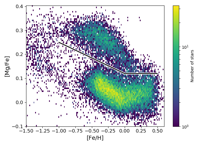
Figure 1: Density in the $[{\rm Mg/Fe}]$ vs. $[{\rm Fe/H}]$ plane for our full sample of 20,485 stars. The black line marks our adopted division between “high-$\alpha$” and “low-$\alpha$” populations. Recognizing that the physical distinction between these populations is the amount of iron enrichment from SNIa, we refer to them through most of the paper as “low-[Fe/Mg]” and “high-[Fe/Mg],” respectively.

3 Abundance ratio maps

3.1 Abundances relative to Mg

Many studies of multi-element stellar abundances examine distributions of [X/Fe] vs. [Fe/H]. Here we choose Mg as our reference element instead of Fe, so our basic diagrams are [X/Mg] vs. [Mg/H]. Because Mg is produced almost entirely by CCSN, it is a simpler tracer of chemical enrichment than Fe, and it has the same meaning (total enrichment from CCSN) on both the high-$\alpha$ and low-$\alpha$ sequences. While oxygen would also be a suitable reference element, we choose Mg because it is more robustly measured in APOGEE (where O measurements come largely from OH and CO lines and are more sensitive to $T_{\rm eff}$) and because it is more accessible to optical surveys. Jönsson et al. (2018) find that Mg is APOGEE’s most accurately measured $\alpha$ element relative to external measurements. Other authors have used Mg as a reference element in abundance ratio studies with similar motivation (e.g., Wheeler et al. 1989; Timmes et al. 1995; Fuhrmann 1998; Cayrel et al. 2004). In a similar spirit, we refer to the high-$\alpha$ and low-$\alpha$ populations hereafter as low-[Fe/Mg] and high-[Fe/Mg], respectively, since the physical distinction between them arises from the absence or prevalence of SNIa iron enrichment rather than an enhancement of $\alpha$ elements relative to CCSN iron. (One could more simply say low-iron and high-iron, but it is the iron relative to $\alpha$-elements that matters for our purposes, so we adopt the more specific terms to avoid confusion.) We examine median abundance ratio trends separately for these two populations, and we find that the combination of this practice and our choice of reference element greatly simplifies the description of abundance trends as a function of Galactic position.

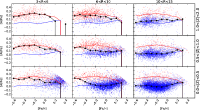
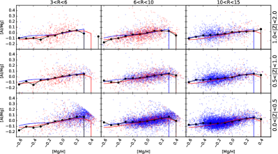
Figure 2: (Left) Distribution of sample stars in [Al/Fe] vs. [Fe/H] in nine Galactic zones, with radial ranges $R/\,{\rm kpc}=3-6$ (left column), $6-10$ (middle column), $10-15$ (right column) and vertical positions $|Z|/\,{\rm kpc}=0-0.5$ (bottom row), $0.5-1$ (middle row), $1-2$ (top row). Red and blue points show stars in the low-[Fe/Mg] (high-$\alpha$) and high-[Fe/Mg](low-$\alpha$) populations, respectively, based on the division marked in Figure 1. Large points connected by the black solid line show the median [Al/Fe] in bins of [Fe/H] in each Galactic zone. Red and blue curves show the median trends for the two populations in the full sample; these curves are the same in all panels. (Right) Same as the left panels, but with Mg rather than Fe as the reference element.

Figure 2 illustrates this simplification for the case of Al. The left half of the figure shows [Al/Fe] vs. [Fe/H] for all sample stars in nine zones of $R,|Z|$, with red and blue points marking stars in the low-[Fe/Mg] (high-$\alpha$) and high-[Fe/Mg] (low-$\alpha$) populations, respectively. Large points connected by the black line show the median abundance ratio of all stars in bins of [Fe/H]. This median trend changes shape with Galactic position, and its shape has no obvious physical interpretation. The scatter about the median trend is large at all locations. However, the median trends for the low-[Fe/Mg] and high-[Fe/Mg] populations individually (red and blue curves) are nearly independent of location, and the scatter about the median trend within each population is fairly small. The changing shape of full sample median reflects the changing ratio of low-[Fe/Mg] to high-[Fe/Mg] stars as a function of Galactic position and metallicity. Put simply, thin-disk stars have low [Al/Fe] at a given [Fe/H] because they have extra Fe from SNIa enrichment, and the median [Al/Fe] vs. [Fe/H] is therefore shaped by the ratio of thin-disk to thick-disk stars.

The right half of the figure plots [Al/Mg] vs. [Mg/H] for the same stars in the same zones. With Mg rather than Fe as reference element, the median trends are nearly identical for low-[Fe/Mg] and high-[Fe/Mg] stars, which is expected because Al production is dominated by CCSN and thus unaffected by the presence of SNIa iron. The full sample median, shown by the large points and black line, is nearly independent of position. The trend is physically sensible for an odd-$Z$ element such as Al: the [Al/Mg] ratio rises with increasing [Mg/H] because the yield of odd-$Z$ elements increases with metallicity. Some other elements exhibit significantly different trends in the two populations because of differing SNIa contributions, but the near independence of Galactic position continues to hold.

3.2 Dual chemical sequences in [Fe/Mg]

Figure 3 plots the distribution of stars in [Fe/Mg] and [Mg/H], now in six radial zones and the same three vertical zones. Small points show stars in the low-[Fe/Mg] population (red) and high-[Fe/Mg] population (blue). In each zone, large points show the median [Fe/Mg] in bins of [Mg/H] for the two populations. Points are plotted only if a bin contains at least 15 stars in a given population. Red and blue curves (the same in each panel) show median relations for the entire sample.

This figure is similar to figure 4 of H15, but our choice of Mg as reference element inverts the $y$-axis and rescales the $x$-axis. Numerous studies show that the low-[Fe/Mg] population is more prominent at small $R$ and large $|Z|$ — i.e., the chemically defined thick disk has a smaller scale length and larger scale height (Bensby et al. 2011; Bovy et al. 2012; Cheng et al. 2012a; Mikolaitis et al. 2014; Nidever et al. 2014; H15). In the high-[Fe/Mg] (thin-disk) population, the mode of [Mg/H] shifts from roughly $+0.3$ in the inner Galaxy to roughly $-0.3$ in the outer Galaxy (see Fig. 22 below), reflecting the stellar metallicity gradient. Radial trends in the low-[Fe/Mg] population are weaker, though in the inner disk the $[{\rm Mg}/{\rm H}]$ distribution shifts to higher metallicity with decreasing $|Z|$. Most importantly from the point of view this paper, the median trends of $[{\rm Fe}/{\rm Mg}]$ with $[{\rm Mg}/{\rm H}]$ for the two populations are nearly constant throughout the disk, as shown by the close agreement between the points in each zone and the corresponding curves. This constancy of the low-[Fe/Mg] and high-[Fe/Mg] locus confirms similar findings by Nidever et al. (2014) and H15 with the larger sample and improved measurements of the DR14 data set. There are small shifts in the median locus of high-[Fe/Mg] stars at $|Z|=1-2\,{\rm kpc}$, a point we discuss further in §5.6 below.

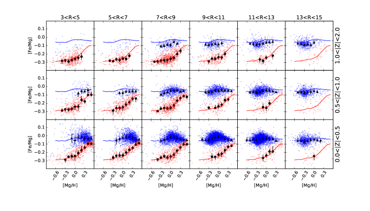
Figure 3: [Fe/Mg] vs [Mg/H] for 18 Galactic zones: from left to right, $R/\,{\rm kpc}=$3-5, 5-7, 7-9, 9-11, 11-13, 13-15; from top to bottom, $|Z|/\,{\rm kpc}=$1-2, 0.5-1, 0-0.5. Red and blue points show stars in the low-[Fe/Mg] and high-[Fe/Mg] populations, respectively. Large black points show the median [Fe/Mg] in 0.1-dex bins of [Mg/H] for each population in each zone, with triangles showing the high-[Fe/Mg] population and circles the low-[Fe/Mg] population; red and blue curves show corresponding median relations for the full sample. For each zone, points are plotted only if an [Mg/H] bin has at least 15 stars. Error bars denote the interquartile range of [Fe/Mg] for the stars in each bin. The statistical errors in the median are much smaller than this range (by $\sim\sqrt{N_{\rm stars}}$).

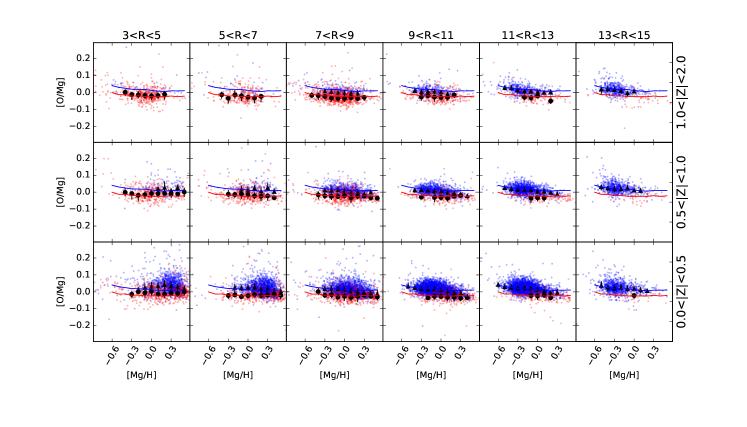
Figure 4: Same as Figure 3, but for [O/Mg].

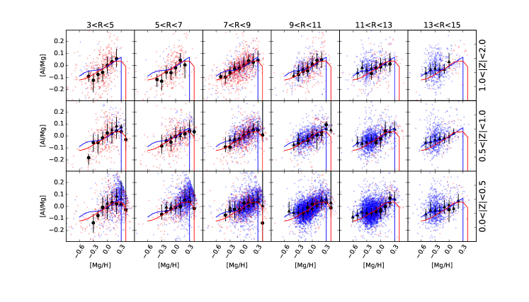
Figure 5: Same as Figure 3, but for [Al/Mg].

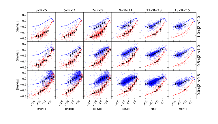
Figure 6: Same as Figure 3, but for [Mn/Mg].

Figure 4 shows a similar map of abundance ratio trends for [O/Mg] vs. [Mg/H]. Like Mg, O is an $\alpha$-element whose production should be dominated by CCSN. The behavior is remarkably simple: for both low-[Fe/Mg] and high-[Fe/Mg] populations, median trends are nearly flat at $[{\rm O/Mg}]=0$ at all Galactic positions. This flatness indicates that IMF-averaged yields of Mg and O are independent of metallicity over the range investigated here, or at least that any metallicity dependence is the same for the two elements. In the full-sample median, the trend for low-[Fe/Mg] stars is offset from that of high-[Fe/Mg] stars by about $-0.02\,$dex in [O/Mg]. We cannot be certain that this small offset is not an artifact of abundance measurement systematics that differ in the two populations. The abundance of oxygen is determined largely from OH lines and its value is sensitive to $T_{\rm eff}$; Jönsson et al. (2018) discuss possible metallicity dependent systematics in $T_{\rm eff}$. However, we have checked that the distributions of $T_{\rm eff}$ and $\log g$ are nearly identical for the low-[Fe/Mg] and high-[Fe/Mg] subsets of our sample, so there is no obvious reason for $T_{\rm eff}$-dependent systematics to produce an offset in [O/Mg] between the populations.

Figure 5 shows results for [Al/Mg] in the same format, while Figure 6 shows results for Mn, an odd-$Z$ element near the iron peak. As seen previously in Figure 2, the median trends for Al show an increasing [Al/Mg] towards higher [Mg/H] as expected for an element whose yield increases with metallicity. The trends for low-[Fe/Mg] and high-[Fe/Mg] stars are nearly identical, consistent with Al having no significant SNIa contribution, and they are independent of Galactic position within the statistical noise of our sample. For Mn, on the other hand, the metallicity dependence is stronger and the trends for low-[Fe/Mg] and high-[Fe/Mg] stars are offset and have different slopes. The higher [Mn/Mg] in high-[Fe/Mg] stars is a sign that a substantial fraction of Mn is produced in SNIa, again consistent with theoretical expectations (see further discussion below). The trends within each population are again nearly independent of Galactic position. At high $|Z|$ the [Mn/Mg] trend of the high-[Fe/Mg] population lies below the global median trend by 0.05-0.1 dex, a larger difference than seen for Fe, O, or Al, but small compared to the separation from the low-[Fe/Mg] trend.

For the other elements considered, median trends are also nearly independent of Galactic position. In §5.6 we will discuss the small deviations from this universal behavior, but we turn first to a discussion and characterization of the global median trends and their interpretation.

4 Global trends and their implications

Given the approximate constancy of the median sequences, we investigate the nucleosynthetic trends by combining all of the data from different zones into single diagrams. To maximize the accuracy, we restrict this combined sample to stars with ${\rm SNR}>200$ per pixel; an advantage of large samples is the ability to choose stars with the highest quality data. This high-SNR subsample still spans the full range of $R$ and $|Z|$, though relative to the full sample it has a smaller fraction of stars at small and large $R$. As an additional check for systematic effects in the abundance measurements, we have examined the trends for the coolest stars in our high-SNR subsample ($T_{\rm eff}<4000\,{\rm K}$, approximately 13% of the total) and for the hottest stars ($T_{\rm eff}>4400\,{\rm K}$, approximately 9% of the total). In general we find no significant difference in global trends for these coolest and hottest subsets, with the exception of Al and V, discussed in §4.2 and §4.3, respectively.

Our discussion of nucleosynthetic sources for different elements is based on that of Andrews et al. (2017, see their §4.2 and Appendix B), which is in turn derived from CCSN yields of Chieffi & Limongi (2004) and Limongi & Chieffi (2006), SNIa yields from the W70 model of Iwamoto et al. (1999), and AGB yields from Karakas (2010). As a useful intuitive reference, we show in Figure 7 a version of the periodic table constructed by J. Johnson and I. Ivans, in which individual elements are color-coded according to their production mechanisms. This coding is informed by both theoretical predictions and empirical data, but it is necessarily uncertain; for example, the attribution of heavy $r$-process elements to neutron star mergers remains a conjecture, strengthened by the spectroscopic observations of the neutron star merger event GW170817 (Pian et al., 2017). For the elements examined in this paper, one can see from the figure that O, Na, Mg, and Al are thought to originate almost entirely from CCSN, that Si, P, S, K, and Ca are thought to come predominantly from CCSN but with significant SNIa contributions, and that V, Cr, Mn, Fe, Co, and Ni are thought to come at least 50% from SNIa, though with significant CCSN contributions in each case. These characterizations apply to solar system abundances; at low metallicity, the relative contributions of SNIa would be lower, and contributions could be different in a galaxy or stellar population with a different IMF or a radically different star formation history. The more detailed calculations presented by Andrews et al. (2017) present a similar picture and show predictions as a function of [Fe/H]. Figure 13 of Rybizki et al. (2017) is another useful reference for relative CCSN, SNIa, and AGB contributions to different elements, with two different yield sets.

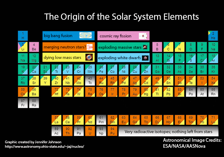
Figure 7: Periodic table of elements color-coded by nucleosynthetic origin, for solar system abundance ratios. Green and light blue represent contributions from CCSN and SNIa, respectively, which dominate the production of elements considered in this paper. Yellow represents contribution from AGB stars. Heavy $r$-process elements are here attributed to merging neutron stars, though the extent to which these dominate $r$-process production remains uncertain. Elements in gray have short radioactive decay times, so terrestrial incidence of these elements does not originate in stellar sources. B, Be, and some Li are produced by cosmic ray spallation. Essentially all H, most He, and some Li originate in the hot early universe.

4.1 $\alpha$-elements

Figure 8 plots [X/Mg] vs. [Mg/H] for the $\alpha$-elements O, Si, S, and Ca. For an element produced purely by CCSN with metallicity-independent IMF-averaged yield, the [X/Mg] ratio is expected to be independent of [Mg/H], and it should be the same for low-[Fe/Mg] and high-[Fe/Mg] stars (see further discussion at the end of §5.5). This is nearly the case for O, though there is a slight offset between the two sequences and a slightly elevated [O/Mg] at low metallicities. For Si the metallicity trend is stronger and more continuous, and the separation of the two sequences is larger, consistent with the moderate SNIa contribution expected for Si. However, while the expected SNIa contribution (relative to CCSN) is larger for S than for Si, we find no separation between the two [S/Mg] sequences. Ca is expected to have the largest SNIa contribution among these elements, and it shows the largest separation between the low-[Fe/Mg] and high-[Fe/Mg] populations. We quantify the relative CCSN vs. SNIa contributions and the metallicity dependence of these contributions in §5 below.

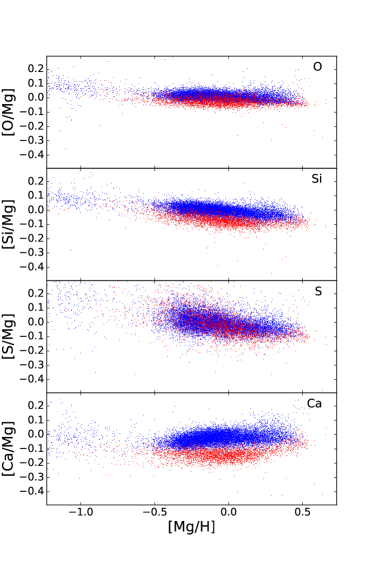
Figure 8: [X/Mg] vs. [Mg/H] for $\alpha$-elements, for all sample stars with ${\rm SNR}>200$. Red and blue points show the low-[Fe/Mg] and high-[Fe/Mg] populations, containing 2038 and 11,311 stars, respectively.

The possibility of systematics in APOGEE oxygen measurements was mentioned in §3.2. For Si, S, and Ca, Jönsson et al. (2018) show that the APOGEE measurements are in fairly good agreement with independent estimates from optical spectra of the same stars, and that the global loci of [X/Fe] vs [Fe/H]  for these elements are in generally good agreement with loci determined independently in local samples.

For a more direct comparison to our [X/Mg]-[Mg/H] distributions, we have used the samples of Adibekyan et al. (2012) and Bensby et al. (2014) and applied the [Mg/Fe] criterion of Equation (1) to define two populations. Figure 9 plots individual stars from the two optical samples over contours that show the density of stars in our full APOGEE DR14 disk sample. In contrast to the Jönsson et al. (2018) star-by-star comparisons, the stars in the optical samples are different from those in the APOGEE data. The Adibekyan et al. (2012) data do not include oxygen abundances, and neither data set includes sulfur abundances.

The Bensby et al. (2014) data show a sloped trend of [O/Mg] vs. [Mg/H], in contrast to the flat trends found in the APOGEE data set. Given the challenges of inferring oxygen abundances from either optical spectra (principally non-LTE corrections) or near-IR spectra (principally the impact of $T_{\rm eff}$ on OH molecular abundances), we cannot be sure which of these trends is more accurate. The APOGEE trend is much easier to understand physically, since Mg and O are both produced mainly during hydrostatic evolution in high mass progenitors of CCSN, and it is not clear what mechanism could create a metallicity-dependent [O/Mg] ratio.

For [Si/Mg] the APOGEE data are in good agreement with the Adibekyan et al. (2012) sample and fair agreement with the Bensby et al. (2014) sample. Without separating the two populations, either of the optical samples might suggest a rising trend of [Si/Mg] with [Mg/H], but the APOGEE data show that the trends are slightly falling within each population. In the solar neighborhood optical samples, the low-[Fe/Mg] stars are preferentially lower [Mg/H], leading to the net rising trend. A trend of [Si/Fe] vs. [Fe/H] would be further complicated by the differing [Fe/Mg] ratios of the two populations.

For [Ca/Mg] the APOGEE data are in good agreement with the Bensby et al. (2014) data. The Adibekyan et al. (2012) data show slightly higher [Ca/Mg] for the low-[Fe/Mg] population and an extension to high [Ca/Mg] for lower metallicity stars in the high-[Fe/Mg] population.

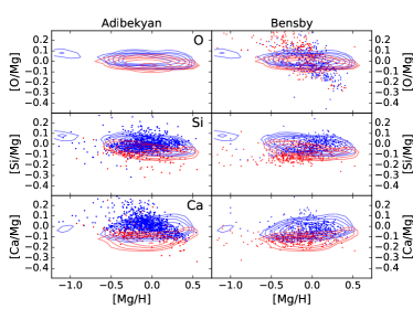
Figure 9: Comparison of APOGEE loci in [X/Mg] vs. [Mg/H] to optical abundance measurements of solar neighborhood stars from Adibekyan et al. (2012) and Bensby et al. (2014), for O, Si, and Ca. Logarithmically spaced red and blue contours show the density of low-[Fe/Mg] and high-[Fe/Mg] stars, respectively, from the APOGEE disk sample. Points show individual stars from the optical samples, with the same color coding. The Adibekyan et al. (2012) data set does not have O abundances, and neither data set has S abundances.

4.2 Light odd-$Z$ elements

Figure 10 plots [X/Mg] vs. [Mg/H] for Na, Al, P, and K, elements with odd atomic number whose production is dominated by CCSN. Predicted yields for these light odd-$Z$ elements increase with stellar metallicity because their production requires a neutron excess, and this excess requires elements heavier than H and He (Truran & Arnett, 1971; Timmes et al., 1995; Woosley et al., 2002). Specifically, higher initial CNO abundances in CCSN progenitors lead to more ${}^{14}{\rm N}$ production during hydrogen burning, the ${}^{14}{\rm N}$ is converted to ${}^{22}{\rm Ne}$ during helium burning, and destruction of ${}^{22}{\rm Ne}$ by $\alpha$-captures becomes a source of free neutrons.

Our results for Al are in qualitative agreement with expectations, with [Al/Mg] increasing with [Mg/H] and similar trends for low-[Fe/Mg] and high-[Fe/Mg] populations. Trends for [K/Mg] are nearly flat, though slightly increasing. For both Na and P we find large differences in [X/Mg] for the low-[Fe/Mg] and high-[Fe/Mg] populations, counter to expectations if production of these elements is dominated by CCSN. We caution that our typical abundance errors for these elements are relatively large even for these ${\rm SNR}>200$ spectra, ranging from 0.05 to 0.2 dex for Na and 0.05 to 0.1 dex for P depending on $T_{\rm eff}$ and [M/H].

There is an obvious artifact in the $[{\rm Na/Mg}]-[{\rm Mg}/{\rm H}]$ diagram: a diagonal gap that corresponds to a narrow but sharp minimum in the [Na/H] distribution at $[{\rm Na/H}]\approx 0-0.1$, which is most pronounced for stars with $\log g<1.5$. This feature is not present in APOGEE DR12 or DR13 [Na/H] abundances; stars with $[{\rm Na/H}]$ in this range in DR12 or DR13 are assigned systematically higher $[{\rm Na/H}]$ in DR14. Despite an extensive investigation, we do not fully understand the origin of this artifact, but it highlights the fact that APOGEE sodium abundance measurements rely on two fairly weak lines, one of which is significantly blended with a CO feature.

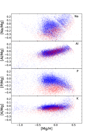
Figure 10: Same as Figure 8 for light odd-$Z$ elements.

As discussed by Jönsson et al. (2018), the APOGEE measurements for Na and Al are generally in good agreement with independent optical measurements for the same stars, and the loci in [Na/Fe]-[Fe/H] and [Al/Fe]-[Fe/H] are similar to those found in local studies. Figure 11 shows [Na/Mg] and [Al/Mg] comparisons to the Adibekyan et al. (2012) and Bensby et al. (2014) samples, indicating reasonable agreement, somewhat better for Bensby et al. (2014) than for Adibekyan et al. (2012). P is relatively unstudied, so there is little in the way of external validation. For K, Jönsson et al. (2018) find substantial systematic differences with measurements made from optical spectra, so our K results should be interpreted with caution.

For Al specifically, we find that the coolest stars in our sample ($T_{\rm eff}<4000\,{\rm K}$) imply a steeper trend of [Al/Mg] vs. [Mg/H]; the median [Al/Mg] of these stars matches that of the full sample near $[{\rm Mg}/{\rm H}]=0$, but it is slightly higher at high-[Mg/H] and lower by about 0.05 dex at $[{\rm Mg}/{\rm H}]\approx-0.3$. The visually estimated trend slope through the main locus of points is about 0.20 for the full sample and about 0.35 for the coolest stars (precise numbers depend on binning and trimming of outliers, especially for the smaller cool, subset). The hottest stars ($T_{\rm eff}>4400\,{\rm K}$) have slightly higher median [Al/Mg] (by about 0.05 dex) at $[{\rm Mg}/{\rm H}]\approx-0.3$; it is difficult to translate this difference into a trend slope because there are few hot stars in our sample with $[{\rm Mg}/{\rm H}]>0$. Neither the coolest nor hottest subsamples show an offset of [Al/Mg] between the low-[Fe/Mg] and high-[Fe/Mg] populations, so the inference that Al production is dominated by CCSN remains robust.

For the other $\alpha$-elements and light odd-$Z$ elements, we find no clear differences in median trends for the coolest or hottest stars in the sample, within the limits set by sample size and scatter in the abundance ratios.

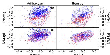
Figure 11: Same as Figure 9 but for Na and Al. The Adibekyan et al. (2012) and Bensby et al. (2014) data sets do not include P or K measurements.

4.3 Iron-peak elements

Figure 12 plots [X/Mg] vs. [Mg/H] for V, Cr, Mn, Fe, Co, and Ni, all “iron-peak” elements for which SNIa are expected to contribute much of the enrichment. Starting with [Fe/Mg], we see the familiar two sequences and the gap between them at sub-solar [Mg/H], though the perfect separation of red and blue points is a consequence of our defining the boundary between the two populations in this plane. The plateau of the low-[Fe/Mg] sequence is at $[{\rm Fe}/{\rm Mg}]\approx-0.3$. The median trend of the high-[Fe/Mg] sequence is almost flat, though here as in other studies (e.g., Casagrande et al. 2011) we find a “banana-shaped” boundary in which the highest [Fe/Mg] stars are concentrated at solar or slightly sub-solar [Mg/H], and the upper envelope of the population falls slightly at higher and lower [Mg/H]. Trends for Ni are similar to those for Fe, but the separation of the two populations is smaller, suggesting a larger relative CCSN contribution for Ni (see further discussion in §5).

V, Mn, and Co have odd atomic numbers, and all three of these elements show increasing [X/Mg] with increasing [Mg/H]. The metallicity-dependence is strongest and the separation of the two populations largest for Mn, while Co has the weakest dependence and smallest population separation. It is not obvious that classic CCSN nucleosynthesis models predict a metallicity dependence for odd-$Z$ iron group elements (see §VIII.D of Woosley et al. 2002). Cr is an even-$Z$ element, and the [Cr/Mg] tracks are for the most part similar to the [Fe/Mg] tracks. However, there is a significant downturn of [Cr/Mg] at super-solar [Mg/H], suggesting that yields become metallicity-dependent in this regime.

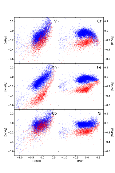
Figure 12: Same as Figure 8 for iron-peak elements. Elements in the left column have odd atomic numbers; those in the right column have even atomic numbers.

APOGEE abundances for V, Cr, and Ni are generally consistent with independent optical analyses of the same stars (Jönsson et al., 2018), and they exhibit similar [X/Fe]-[Fe/H] trends to those in local samples. APOGEE performs an internal calibration designed to remove abundance trends with $T_{\rm eff}$ in open clusters. This $T_{\rm eff}$ correction is relatively large for Co, leaving more room for systematic errors in Co abundances induced by metallicity-dependent systematics in $T_{\rm eff}$. APOGEE [Co/H] ratios also have significant scatter and a weak metallicity trend relative to optical measurements. For Mn, APOGEE measurements agree with independent analyses using similar methodology. However, applying non-LTE corrections to Mn abundances flattens the observed trend of [Mn/Fe] with [Fe/H] by boosting Mn at lower metallicity (Bergemann & Gehren, 2008; Battistini & Bensby, 2015). APOGEE measurements match the optical measurements without non-LTE corrections.

Figure 13 shows [X/Mg]-[Mg/H] comparisons to the Adibekyan et al. (2012) and Bensby et al. (2014) samples for iron-peak elements. For V, Mn, and Co, we take values from Battistini & Bensby (2015), who present measurements for a subset of the Bensby et al. (2014) stars. Agreement for the iron-peak elements is generally good, with the most significant difference being the lowest [Ni/Mg] values in the Bensby et al. (2014) sample. The separation between the low-[Fe/Mg] and high-[Fe/Mg] populations in [V/Mg] and [Mn/Mg] is also smaller for the Battistini & Bensby (2015) data than for the APOGEE data.

For the coolest stars in the sample ($T_{\rm eff}<4000\,{\rm K}$), we find that the [V/Mg]-[Mg/H] trends are shifted upward by about 0.1 dex relative to that of the full sample. The slopes of these trends and the separation between the low-[Fe/Mg] and high-[Fe/Mg] populations remain similar. For other iron-peak elements, the trends for the coolest stars show no obvious offsets or slope differences relative to the full sample. The hottest stars ($T_{\rm eff}>4400\,{\rm K}$) have slightly higher ($\sim 0.05-0.1$ dex) [V/Mg] at $[{\rm Mg}/{\rm H}]\approx-0.3$ but show no other obvious offsets or slope differences.

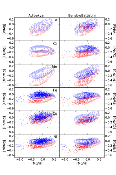
Figure 13: Same as Figure 9 but for iron-peak elements. The Adibekyan et al. (2012) data set does not include V, Cr, or Mn. In the right column, results for V, Co, and Mn come from Battistini & Bensby (2015).

5 A semi-empirical model of element yields

5.1 Model definition

As a semi-empirical description of our observed trends that incorporates basic physical expectations about the origin of these elements, we adopt a “2-process model” in which each star’s abundances are represented as the sum of a “core collapse process” with amplitude $A_{\rm cc}$ and an “SNIa process” with amplitude $A_{\rm Ia}$, with these amplitudes multiplying coefficients $p^{X}$ that are specific to each element. The abundance of element $X$ is

$$\left({{\rm X}\over{\rm H}}\right)=A_{\rm cc}p_{\rm cc}^{X}(Z)+A_{\rm Ia}p_{\rm Ia}^{X}(Z)~{}.$$ (2)

The dependence of each process $p_{\rm cc}^{X}$ and $p_{\rm Ia}^{X}$ on $Z$ allows for metallicity-dependent IMF-averaged yields of element X. The model makes no specific assumption about the chemical evolution history that leads to a given star’s value of $A_{\rm cc}$ and $A_{\rm Ia}$ (see further discussion in §5.5). Our comments about theoretical expectations throughout this section are again based on the references discussed at the beginning of §4.

We normalize $A_{\rm cc}=1$ at solar abundance, so

$$p_{\rm cc,\odot}^{X}\equiv p_{\rm cc}^{X}(Z_{\odot})=\left({{\rm X}\over{\rm H}}\right)_{{\rm cc},\odot}$$ (3)

is the contribution of core collapse supernovae to the solar abundance ratio of element X. With this normalization, one can take $({\rm X}/{\rm H})$ to represent either a number density ratio or a mass-fraction ratio. We assume (1) that Mg is a pure CCSN element with an IMF-averaged yield that is independent of metallicity, (2) that the IMF-averaged CCSN and SNIa iron yields are independent of metallicity, and (3) that the observed high-$\alpha$ plateau at $[{\rm Mg/Fe}]=+0.3$ corresponds to pure CCSN enrichment. One can therefore infer $A_{\rm cc}$ and $A_{\rm Ia}$ for a given star from its Mg abundance and its [Mg/Fe] ratio:

$$A_{\rm cc}=10^{[{\rm Mg}/{\rm H}]}~{},$$ (4)

$${A_{\rm cc}\over A_{\rm cc}+A_{\rm Ia}}=10^{[{\rm Mg/Fe}]-0.3}~{},$$ (5)

or equivalently

$${A_{\rm Ia}\over A_{\rm cc}}=10^{0.3-[{\rm Mg/Fe}]}-1~{}.$$ (6)

Since $10^{0.3}\approx 2$, Equation (6) implies that $A_{\rm Ia}\approx A_{\rm cc}=1$ for a star with solar abundances.

In principle one can generalize this model to allow metallicity-dependent Mg or Fe yields or a different plateau value of [Mg/Fe], but we will not do so here. For other elements we do allow metallicity dependence, which for simplicity we model as power laws of slopes $\alpha_{\rm cc}$ and $\alpha_{\rm Ia}$ between abundance and (Mg/H):

$$p_{\rm cc}^{X}(Z) = p_{\rm cc,\odot}^{X}\cdot 10^{\alpha_{\rm cc}[{\rm Mg}/{\rm H}]}$$ (7)

$$p_{\rm Ia}^{X}(Z) = p_{\rm Ia,\odot}^{X}\cdot 10^{\alpha_{\rm Ia}[{\rm Mg}/{\rm H}]}~{}.$$ (8)

For each element, there are three model parameters: the slopes $\alpha_{\rm cc}$ and $\alpha_{\rm Ia}$ and the relative SNIa contribution at solar metallicity, described by the ratio

$$R^{X}_{\rm Ia}\equiv\frac{p_{\rm Ia,\odot}^{X}}{p_{\rm cc,\odot}^{X}}~{}.$$ (9)

The normalization convention of Equation (3) together with $A_{{\rm Ia},\odot}=A_{{\rm cc},\odot}=1$ implies

$$p_{\rm cc,\odot}^{X}+p_{\rm Ia,\odot}^{X}=\left({{\rm X}\over{\rm H}}\right)_{\odot}~{}.$$ (10)

The ratio $A_{\rm Ia}/A_{\rm cc}$ (eq. 6) describes the relative contribution of the SNIa and CCSN processes to a given star, while $R^{X}_{\rm Ia}$ describes the relative contribution of these two processes to a given element X at solar [Mg/H]. Our model assumptions (1) and (2) correspond to parameter values $R_{\rm Ia}^{{\rm Mg}}=\alpha_{\rm cc}^{{\rm Mg}}=\alpha_{\rm Ia}^{{\rm Mg}}=0$ and $\alpha_{\rm cc}^{{\rm Fe}}=\alpha_{\rm Ia}^{{\rm Fe}}=0$, respectively, while assumption (3) implies $R_{\rm Ia}^{{\rm Fe}}=1$. The metallicity dependence of an $[{\rm X/Mg}]-[{\rm Mg}/{\rm H}]$ trend is related to but not the same as the implied metallicity dependence of the yield of element $X$, a point we discuss further in §5.5.

Once the model parameters are determined, one can use a star’s measured [Mg/H] and [Mg/Fe] to predict the abundances of other elements. Specifically, because $p^{\rm Mg}_{\rm Ia}=\alpha_{\rm cc}^{{\rm Mg}}=0$, one has a relation for the ratio

$$\left({X\over{\rm Mg}}\right)={A_{\rm cc}p_{\rm cc}^{X}(Z)+A_{\rm Ia}p_{\rm Ia}^{X}(Z)\over A_{\rm cc}p^{\rm Mg}_{\rm cc}}~{}.$$ (11)

Scaling to solar abundances and using $(A_{\rm cc}/A_{\rm Ia})_{\odot}=1$ gives

$${({\rm X}/{\rm Mg})\over({\rm X}/{\rm Mg})_{\odot}} ={p_{\rm cc}^{X}(Z)+(A_{\rm Ia}/A_{\rm cc})p_{\rm Ia}^{X}(Z)\over p_{\rm cc}^{X}(Z_{\odot})+p_{\rm Ia}^{X}(Z_{\odot})}$$ (12)

$$={p_{\rm cc}^{X}(Z)\over p_{\rm cc}^{X}(Z_{\odot})}\times{1+(A_{\rm Ia}/A_{\rm cc})p_{\rm Ia}^{X}(Z)/p_{\rm cc}^{X}(Z)\over 1+p_{\rm Ia}^{X}(Z_{\odot})/p_{\rm cc}^{X}(Z_{\odot})}~{}.$$ (13)

One can combine this result with the definitions (7)-(9) to obtain

$$[{\rm X}/{\rm Mg}] =\alpha_{\rm cc}[{\rm Mg}/{\rm H}]$$

$$+\log\left[{1+R^{X}_{\rm Ia}(A_{\rm Ia}/A_{\rm cc})\cdot 10^{(\alpha_{\rm Ia}-\alpha_{\rm cc})[{\rm Mg}/{\rm H}]}\over 1+R^{X}_{\rm Ia}}\right]~{},$$ (14)

where the value of $A_{\rm Ia}/A_{\rm cc}$ is inferred from the [Mg/Fe] ratio via Equation (6).

For a pure CCSN element, with $R^{X}_{\rm Ia}=0$, Equation (14) implies $[{\rm X/Mg}]=\alpha_{\rm cc}[{\rm Mg}/{\rm H}]$. If the metallicity dependence is also $\alpha_{\rm cc}=0$, the element simply tracks Mg, with $[{\rm X/Mg}]=0$ for all stars regardless of their SNIa enrichment. For any element with metallicity-independent yields, Equation (14) simplifies to

$$[{\rm X}/{\rm Mg}]=\log\left[{{1+R^{X}_{\rm Ia}(A_{\rm Ia}/A_{\rm cc})}\over{1+R^{X}_{\rm Ia}}}\right]~{},$$ (15)

which leads to $[{\rm X/Mg}]=-\log(1+R^{X}_{\rm Ia})$ for a “plateau” star with no SNIa enrichment and $[{\rm X/Mg}]=0$ for any star with equal SNIa and CCSN amplitudes ($A_{\rm Ia}/A_{\rm cc}=1$). For example, Fe has $R^{X}_{\rm Ia}=1$, and Equation (15) implies $[{\rm Fe}/{\rm Mg}]=-0.3$ for pure CCSN enrichment and $[{\rm Fe}/{\rm Mg}]=0$ for equal SNIa and CCSN contributions.

5.2 $\alpha$-elements

The parameters of the 2-process model, different for each element, can in principle be fit to the entire sample of stars, without dividing them into low-[Fe/Mg] and high-[Fe/Mg] populations. Here, however, we fit the model to the median sequences of the two populations, i.e., to the median [X/Mg] values of ${\rm SNR}>200$ stars in 0.1-dex bins of [Mg/H] over the range $-0.8\leq[{\rm Mg}/{\rm H}]\leq+0.5$. The median sequences themselves are listed in Tables 1-6. We perform unweighted least-squares fits; since the model is simple and the (tiny) statistical errors on the median abundance ratios are smaller than systematic errors, a weighted $\chi^{2}$ fit is unwarranted. All of the model fits are poor in a formal $\chi^{2}$ sense. We perform one set of fits with the SNIa metallicity index set to $\alpha_{\rm Ia}=0$ so that there are only two parameters, and a second set of fits with free $\alpha_{\rm Ia}$. We find best-fit parameters by a simple grid search with steps of 0.01 in each free parameter, and we do not infer parameter errors because the fits are formally poor and we do not expect the model to be a complete description of the data.

Table 1: Median sequences, $\alpha$-elements, low-[Fe/Mg] stars

[Mg/H]	[O/Mg]	[Si/Mg]	[S/Mg]	[Ca/Mg]
-0.744	0.037	0.061	0.074	-0.108
-0.639	0.010	0.000	0.043	-0.130
-0.541	-0.015	-0.021	0.051	-0.137
-0.437	-0.017	-0.032	0.072	-0.128
-0.349	-0.019	-0.034	0.020	-0.132
-0.254	-0.024	-0.047	0.027	-0.132
-0.146	-0.028	-0.065	0.006	-0.142
-0.050	-0.026	-0.072	-0.032	-0.142
0.044	-0.029	-0.082	-0.046	-0.144
0.146	-0.028	-0.090	-0.073	-0.138
0.237	-0.030	-0.096	-0.089	-0.125
0.346	-0.043	-0.102	-0.108	-0.115
0.448	-0.030	-0.095	-0.099	-0.100

Table 2: Median sequences, $\alpha$-elements, high-[Fe/Mg] stars

[Mg/H]	[O/Mg]	[Si/Mg]	[S/Mg]	[Ca/Mg]
-0.744	0.064	0.051	0.134	-0.042
-0.639	0.036	0.023	0.089	-0.057
-0.541	0.026	0.037	0.051	-0.060
-0.437	0.023	0.029	0.036	-0.055
-0.349	0.019	0.018	0.030	-0.048
-0.254	0.018	0.011	0.015	-0.037
-0.146	0.017	0.006	0.002	-0.022
-0.050	0.015	0.000	-0.008	-0.014
0.044	0.009	-0.011	-0.024	-0.015
0.146	0.002	-0.022	-0.035	-0.018
0.237	-0.000	-0.029	-0.041	-0.017
0.346	-0.011	-0.037	-0.051	-0.015
0.448	-0.024	-0.058	-0.067	-0.033

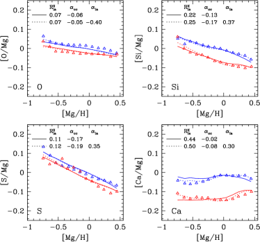
Figure 14: Median sequences and the 2-process model for $\alpha$-elements. Triangles show the median [X/Mg] of stars in 0.1-dex bins of [Mg/H] in the low-[Fe/Mg] (red) and high-[Fe/Mg] (blue) populations, respectively. These sequences are derived from the same set of stars plotted in Figure 8. Solid curves show fits of the 2-process model to the median sequences with the metallicity-dependence of the SNIa contribution set to zero. Dotted curves show fits in which the index $\alpha_{\rm Ia}$ of the SNIa metallicity dependence is free. The fitted values of $R^{X}_{\rm Ia}$, the ratio of amplitudes of the SNIa process to the CCSN process at $[{\rm Mg}/{\rm H}]=0$, are listed in each panel, together with the fitted metallicity slopes $\alpha_{\rm cc}$ and $\alpha_{\rm Ia}$ (see eqs. 7-9). Of these elements, Ca has the largest relative SNIa contribution, and Si and S have the strongest metallicity dependence.

Figure 14 shows results for the $\alpha$-elements, for which the full $[{\rm X/Mg}]-[{\rm Mg}/{\rm H}]$ distributions were shown previously in Figure 8. The small separation of the two [O/Mg] median sequences leads to a small but non-zero value of $R^{X}_{\rm Ia}=0.07$. Even this level of SNIa contribution is higher than theoretically expected. The sequence separation and inferred $R^{X}_{\rm Ia}$ could represent a contribution to O from some other source, such as AGB stars, that has a delayed enrichment time profile resembling that of SNIa. Alternatively, the separation could arise from a systematic error in our oxygen abundance determinations that is correlated with [Fe/Mg], such that we systematically underestimate [O/Mg] in low-[Fe/Mg] stars, though we have not identified a systematic that would lead to this behavior (see previous discussion in §4.1). The median trends show a small but clear metallicity dependence at $[{\rm Mg}/{\rm H}]<-0.3$, but this dependence is not well described by a power law over the full [Mg/H] range so our model does not fit it well.

For Si our fit implies a larger but still sub-dominant SNIa contribution, $R^{X}_{\rm Ia}=0.22-0.25$, qualitatively consistent with expectations. There is a significant trend of decreasing [Si/Mg] with increasing [Mg/H]. The fit with free $\alpha_{\rm Ia}$ better describes the full locus of the high-[Fe/Mg] sequence, but only at the 0.04-dex level, and given the uncertainties of the data and the simplicity of the power-law model it is not clear that this improvement is physically significant. The decreasing yield for CCSN appears more robust, and the inferred slope $\alpha_{\rm cc}$ is similar whether or not $\alpha_{\rm Ia}$ is forced to zero ($-0.13$ vs. $-0.17$). We emphasize again that our model assumes a metallicity-independent yield for Mg by construction, and one should more accurately view the value of $\alpha_{\rm cc}$ as reflecting the metallicity dependence relative to that of Mg.

As previously noted, the similar [S/Mg] of the two populations implies, at face value, very little SNIa contribution to sulfur enrichment; our model fits yield $R^{X}_{\rm Ia}=0.11$ or 0.12. This result runs somewhat counter to theoretical yield models, which predict that the relative SNIa contribution increases, or at least does not decrease, for heavier $\alpha$-elements. The inferred metallicity dependence, $\alpha_{\rm cc}=-0.17$ or $-0.19$, is similar to that for Si. For Ca we infer a larger $R^{X}_{\rm Ia}=0.44-0.50$, as expected for this heavier element, and weaker metallicity dependence. In this case, allowing free $\alpha_{\rm Ia}$ produces a qualitatively better fit for both sequences across the full [Mg/H] range, with inferred $\alpha_{\rm Ia}=0.30$.

O and Mg are produced primarily during the hydrostatic evolution of massive stars, before they explode as CCSN, and their expected yields increase rapidly with progenitor mass. Si and Ca, on the other hand, are produced mainly by explosive nucleosynthesis during the CCSN event itself, and their expected yields are less mass-dependent. The hydrostatic/explosive element ratio can therefore provide a diagnostic of the stellar IMF; for example, McWilliam et al. (2013), Vincenzo et al. (2015), and Carlin et al. (2018) have used this ratio to argue that the IMF in the Sagittarius dwarf galaxy was deficient in high mass stars relative to the Milky Way disk. In principle, the offsets found here for Si and Ca could arise from a change in the IMF between the low-[Fe/Mg] and high-[Fe/Mg] populations. However, given the constancy of these trends through the disk and the clear dependence on [Fe/Mg], it is more natural to associate them with SNIa contributions to these elements, which are theoretically expected in any case. These SNIa contributions should be accounted for when using the hydrostatic/explosive ratio to test for IMF variations, and our 2-process model fits provide a convenient way to do so.

Table 3: Median sequences, odd-$Z$ elements, low-[Fe/Mg] stars

[Mg/H]	[Na/Mg]	[Al/Mg]	[P/Mg]	[K/Mg]
-0.744	…….	-0.156	-0.458	-0.164
-0.639	…….	-0.108	-0.303	-0.120
-0.541	-0.388	-0.122	-0.333	-0.118
-0.437	-0.344	-0.111	-0.285	-0.104
-0.349	-0.329	-0.101	-0.281	-0.101
-0.254	-0.301	-0.065	-0.266	-0.087
-0.146	-0.280	-0.059	-0.284	-0.087
-0.050	-0.226	-0.029	-0.280	-0.077
0.044	-0.230	0.008	-0.274	-0.066
0.146	-0.297	0.024	-0.262	-0.071
0.237	-0.161	0.029	-0.263	-0.062
0.346	-0.110	0.055	-0.279	-0.063
0.448	0.010	……	-0.387	-0.024

Table 4: Median sequences, odd-$Z$ elements, high-[Fe/Mg] stars

[Mg/H]	[Na/Mg]	[Al/Mg]	[P/Mg]	[K/Mg]
-0.744	-0.143	-0.269	0.068	-0.082
-0.639	-0.174	-0.149	-0.013	-0.041
-0.541	-0.137	-0.077	0.019	-0.047
-0.437	-0.112	-0.081	-0.022	-0.054
-0.349	-0.106	-0.059	-0.036	-0.044
-0.254	-0.099	-0.052	-0.040	-0.038
-0.146	-0.091	-0.042	-0.038	-0.030
-0.050	-0.099	-0.025	-0.044	-0.027
0.044	-0.107	0.001	-0.070	-0.028
0.146	0.011	0.024	-0.111	-0.025
0.237	0.069	0.049	-0.148	-0.011
0.346	0.067	0.069	-0.200	0.001
0.448	-0.017	……	-0.256	0.014

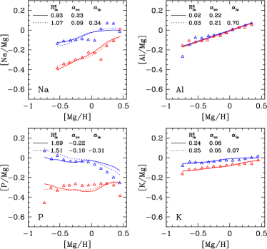
Figure 15: Same as Figure 14 but for light odd-$Z$ elements. The unusual feature in the observed median trend for [Na/Mg] is caused by the analysis artifact discussed in §4.2. Na and P exhibit a large sequence separation implying a large SNIa contribution, contrary to theoretical expectations. Al and K have small inferred SNIa contributions and slowly rising metallicity trends.

5.3 Light odd-$Z$ elements

Figure 15 presents similar median sequences and model fits for the light odd-$Z$ elements. Note that the [X/Mg] axis-range is expanded on these plots relative to the $\alpha$-element plots. For sodium the large gap in [Na/Mg] between the low-[Fe/Mg] and high-[Fe/Mg] sequences implies, in the context of our model, a large SNIa contribution, with inferred $R^{X}_{\rm Ia}=0.93-1.07$. These values imply that slightly over half of the sodium in solar metallicity stars would come from SNIa, in strong disagreement with supernova models. Some Na production from AGB stars is expected (Ventura & D’Antona, 2005; Karakas, 2010), but at least in the calculations of Andrews et al. (2017) and Rybizki et al. (2017) these predicted contributions are much smaller than the CCSN contribution. The broad trend of increasing [Na/Mg] with increasing [Mg/H] is expected for an odd-$Z$ element. The sharp changes of slope near $[{\rm Mg}/{\rm H}]=0$ on both sequences are affected by the previously discussed abundance artifact evident in Figure 10. Unsurprisingly, the power-law metallicity dependence of the model is a poor fit to these median sequences, and the values of $\alpha_{\rm cc}$ and $\alpha_{\rm Ia}$ should be considered unreliable. Statistical errors for the Na abundances are large (mean of 0.068 dex) because the Na lines in the APOGEE spectral range are weak. However, there is no obvious systematic error that would cause a difference of [Na/Mg] for stars in the low-[Fe/Mg] and high-[Fe/Mg] populations, so the implication of a substantial non-CCSN contribution to sodium enrichment appears more robust.

For aluminum we find a low SNIa contribution, with best fit $R^{X}_{\rm Ia}=0.02$, and an increasing metallicity trend with $\alpha_{\rm cc}=0.22$. The temperature effects discussed in §4.2 imply some systematic uncertainty in $\alpha_{\rm cc}$, as the slope for the coolest stars in our sample is steeper than that of the full sample. For potassium we find a larger but sub-dominant SNIa contribution, $R^{X}_{\rm Ia}=0.24$, and a positive but weak metallicity trend, with $\alpha_{\rm cc}=0.06$. Existing supernova yield calculations underpredict observed potassium abundances by a substantial factor (see, e.g., fig. 9 of Andrews et al. 2017 or fig. 14 of Rybizki et al. 2017).

For phosphorous, as for sodium, the large gap between the two median sequences implies a large SNIa contribution in the context of our model, with $R^{X}_{\rm Ia}\approx 1.6$. This is again surprising relative to model predictions (Rybizki et al., 2017), in which CCSN contributions dominate over SNIa and AGB production. The metallicity dependence of the high-[Fe/Mg] sequence is curved and not well fit by our power-law model, even with $\alpha_{\rm cc}$ and $\alpha_{\rm Ia}$ both free to vary. As with sodium, statistical errors (mean of 0.076 dex) and potential systematic errors are large, so we are cautious about drawing physical conclusions from the phosphorous results. However, there is no obvious systematic that would lead to different [P/Mg] ratios for the low-[Fe/Mg] and high-[Fe/Mg] populations.

Table 5: Median sequences, iron-peak elements, low-[Fe/Mg] stars

[Mg/H]	[V/Mg]	[Cr/Mg]	[Mn/Mg]	[Fe/Mg]	[Co/Mg]	[Ni/Mg]
-0.744	-0.403	-0.277	-0.615	-0.298	-0.389	-0.260
-0.639	-0.374	-0.292	-0.566	-0.292	-0.282	-0.215
-0.541	-0.363	-0.303	-0.536	-0.295	-0.244	-0.203
-0.437	-0.355	-0.261	-0.523	-0.285	-0.194	-0.191
-0.349	-0.336	-0.268	-0.499	-0.281	-0.177	-0.182
-0.254	-0.307	-0.257	-0.468	-0.266	-0.136	-0.174
-0.146	-0.273	-0.249	-0.443	-0.263	-0.096	-0.175
-0.050	-0.225	-0.240	-0.402	-0.253	-0.072	-0.171
0.044	-0.193	-0.231	-0.351	-0.236	-0.058	-0.168
0.146	-0.155	-0.215	-0.273	-0.203	-0.052	-0.161
0.237	-0.116	-0.209	-0.206	-0.171	-0.045	-0.146
0.346	-0.044	-0.205	-0.143	-0.151	-0.020	-0.132
0.448	……	-0.233	-0.074	-0.146	0.066	-0.129

Table 6: Median sequences, iron-peak elements, high-[Fe/Mg] stars

[Mg/H]	[V/Mg]	[Cr/Mg]	[Mn/Mg]	[Fe/Mg]	[Co/Mg]	[Ni/Mg]
-0.744	-0.163	-0.123	-0.224	-0.054	-0.221	-0.035
-0.639	-0.194	-0.072	-0.209	-0.067	-0.167	-0.014
-0.541	-0.222	-0.044	-0.178	-0.058	-0.090	0.002
-0.437	-0.204	-0.058	-0.176	-0.062	-0.071	-0.011
-0.349	-0.175	-0.059	-0.164	-0.061	-0.047	-0.018
-0.254	-0.149	-0.049	-0.140	-0.053	-0.037	-0.024
-0.146	-0.125	-0.036	-0.102	-0.037	-0.036	-0.027
-0.050	-0.090	-0.033	-0.063	-0.023	-0.030	-0.026
0.044	-0.051	-0.043	-0.025	-0.022	-0.004	-0.019
0.146	0.007	-0.065	0.010	-0.028	0.031	-0.009
0.237	0.047	-0.096	0.047	-0.035	0.076	-0.004
0.346	-0.034	-0.129	0.082	-0.046	0.125	0.001
0.448	……	-0.165	0.057	-0.066	0.111	-0.018

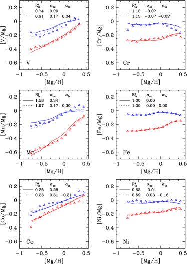
Figure 16: Same as Figure 14 but for iron-peak elements. With the exception of Co, all elements show substantial SNIa contributions, with $R^{X}_{\rm Ia}>0.5$. The odd-$Z$ elements (left column) show strong metallicity trends while the even-$Z$ elements (right column) do not.

5.4 Iron-peak elements

Figure 16 shows median sequences for iron-peak elements, with the odd-$Z$ elements V, Mn, Co, on the left and the even-$Z$ elements Cr, Fe, Ni on the right. By construction the model for Fe has $R^{X}_{\rm Ia}=1.0$, $\alpha_{\rm cc}=\alpha_{\rm Ia}=0.0$, and fits the observed median sequences perfectly. For Cr the inferred process ratio is $R^{X}_{\rm Ia}=1.12$; the metallicity trend is mostly flat, but there is a downturn of [Cr/Mg] at super-solar [Mg/H] in the high-[Fe/Mg] population, similar to the behavior for P. For Ni the inferred $R^{X}_{\rm Ia}=0.63$, implying a larger CCSN contribution. The inferred metallicity dependence is again weak. Note that the median sequence for the low-[Fe/Mg] stars (red points) turns up at high [Mg/H] even with $\alpha_{\rm cc}=\alpha_{\rm Ia}=0$ because the value of [Fe/Mg] is higher, i.e., the upturn reflects the larger contribution of SNIa elements at the high-metallicity end of the low-[Fe/Mg] sequence.

All of the odd-$Z$ iron-peak elements show clear metallicity trends, steeper than those of the light odd-$Z$ elements. The large separation of the median sequences for Mn implies a large SNIa contribution, larger than that of any other element considered here, with $R^{X}_{\rm Ia}=1.58$ (1.97) for the fit with $\alpha_{\rm Ia}=0$ ($\alpha_{\rm Ia}$ free). The inferred $R^{X}_{\rm Ia}$ for V and Co are 0.74 and 0.25, respectively (for $\alpha_{\rm Ia}=0$). In the case of Mn, allowing a metallicity trend for the SNIa process noticeably improves the fit to the observations. For V and Co the improvement is less clear, though the inference of a metallicity-dependent CCSN process is robust.

Battistini & Bensby (2015) have examined [X/Fe] trends for V, Mn, and Co in the local Galactic disk, in comparison to bulge, halo, and globular cluster samples. For Mn they find a significant rise of [Mn/Fe] with increasing [Fe/H], qualitatively similar to our results for [Mn/Mg]. However, the trend largely disappears if they include non-LTE corrections in their Mn abundance determinations. Their trends for V and Co are closer to those of $\alpha$-elements, with decreasing [X/Fe] over the range $-0.8>[{\rm Fe/H}]>0$. In light of our results, it seems that the different behavior of V and Co relative to Mn might be explained by the combination of a lower SNIa fraction and a weaker metallicity dependence. This combination allows an underlying positive metallicity trend to be masked by the trend of higher SNIa iron contribution at higher [Fe/H], analogous to our results for [Al/Fe] shown in Figure 2. However, all three of these element abundances are challenging to measure, so further investigation using both optical and near-IR samples is warranted.

5.5 Relation of median sequences to metallicity-dependent yields

Figs. 14-16 suggest metallicity-dependent yields for some elements, especially the odd-$Z$ elements below and near the iron peak. However, the trend of an element ratio with $[{\rm Mg}/{\rm H}]$ depends on the chemical evolution history as well as on the yield metallicity-dependence itself, because the metals present in the interstellar medium (ISM) at a given time come from stars that formed over a range of previous times, when the composition of the ISM (and thus of newly forming stars) may have been different. Thus, even if the stellar IMF and nucleosynthetic processes within stars remain constant throughout the Galactic disk, one might expect location-dependent trends of [X/Mg] with [Mg/H] because of differences in star formation history, accretion, or outflows. To address this issue, we use one-zone chemical evolution models similar to those of Weinberg et al. (2017); we compute their evolution numerically instead of analytically so that we can include a hypothetical element with a metal-dependent yield. In these models, the predicted [X/Mg]-[Mg/H] trends prove insensitive to details of the evolutionary history, which makes the relation of observed trends to IMF-averaged yields straightforward to interpret and largely explains why we find median sequences that are constant throughout the Galactic disk.

The top row of Figure 17 shows results for four models, each of which assumes a constant star formation efficiency timescale $\tau_{*}\equiv M_{\rm gas}/\dot{M}_{*}=2\,{\rm Gyr}$ and an exponential star formation history $\dot{M}_{*}(t)\propto e^{-t/\tau_{\rm sfh}}$ with $\tau_{\rm sfh}=6\,{\rm Gyr}$. Star formation drives an outflow with mass loading factor $\eta=\dot{M}_{\rm out}/\dot{M}_{*}=5$, 2.5, 1.5, or 0.5, which ejects gas at the current ISM metallicity. We adopt a $t^{-1.1}$ power-law delay time distribution for SNIa (Maoz & Mannucci, 2012; Maoz et al., 2012) with a minimum delay time of $0.15\,{\rm Gyr}$. The left panel shows evolutionary tracks in the $[{\rm Mg/Fe}]-[{\rm Fe/H}]$ plane. As discussed by Andrews et al. (2017) and Weinberg et al. (2017), the abundances of one-zone models with constant parameters typically approach late-time equilibrium values that depend primarily on the element yield and the outflow parameter $\eta$.

The top right panel shows model tracks of $[{\rm X/Mg}]$ vs. $[{\rm Mg}/{\rm H}]$ for an element with IMF-averaged yield

$$y_{\rm X}=y_{\rm Mg}\left(Z_{{\rm X},\odot}/Z_{{\rm Mg},\odot}\right)\times 10^{\alpha_{\rm cc}[{\rm Mg}/{\rm H}]}~{},$$ (16)

where $Z_{{\rm X},\odot}$ is the solar abundance of element X and we have adopted $\alpha_{\rm cc}=0.2$ for this example. We assume that element X is produced entirely by CCSN, so results in this panel are independent of the adopted iron yields and SNIa delay time distribution. At early times the ratio $Z_{\rm X}/Z_{\rm Mg}$ of newly forming stars is lower than the yield ratio $y_{\rm X}/y_{\rm Mg}$, shown by the circles, because much of the ISM enrichment came from stars with metallicity lower than the current ISM value. However, once the $[{\rm Mg}/{\rm H}]$ ratio approaches its equilibrium value, the $[{\rm X/Mg}]$ track bends slightly upward and settles at the value implied by the yield ratio. The $[{\rm X/Mg}]-[{\rm Mg}/{\rm H}]$ tracks are therefore not pure power-laws, and their effective slopes are steeper than those of the yield trend itself. Models with exponential star formation history and a yield slope of 0.20 produce a trend slope of $\alpha_{\rm cc}\approx 0.35$, similar to that inferred for Mn (see Figure 16). The model tracks end at different $[{\rm Mg}/{\rm H}]$ because of the different values of $\eta$, but where they overlap they are nearly identical.

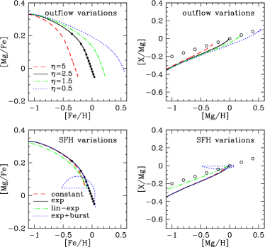
Figure 17: Evolutionary tracks of $[{\rm Mg/Fe}]$ vs. $[{\rm Fe/H}]$ (left panels) and $[{\rm X/Mg}]$ vs. $[{\rm Mg}/{\rm H}]$ (right panels) for a hypothetical CCSN element with a metallicity-dependent yield (eq. 16). Upper panels show models with $\dot{M}_{*}(t)\propto e^{-t/\tau_{\rm sfh}}$, all with $\tau_{\rm sfh}=6\,{\rm Gyr}$ but with four different values of the outflow mass-loading parameter $\eta$ as marked. Circles on the $\eta=2.5$ track in the left panel mark $1\,{\rm Gyr}$ intervals ($t_{\rm max}=12\,{\rm Gyr}$). Circles in the right panel show the value of $[{\rm X/Mg}]$ corresponding to the yield ratio $y_{\rm X}/y_{\rm Mg}$. Models in the lower panels have $\eta=2.5$ and four different star formation histories: constant, exponential with $\tau_{\rm sfh}=6\,{\rm Gyr}$, linear-exponential ($\dot{M}_{*}(t)\propto te^{-t/\tau_{\rm sfh}}$) with the same $\tau_{\rm sfh}$, or exponential with a gas influx and subsequent burst of star formation at $t=6\,{\rm Gyr}$. The predicted trend of [X/Mg] with [Mg/H] is only weakly dependent on the outflow rate or star formation history, and it is close to but steeper than the trend of $y_{\rm X}/y_{\rm Mg}$ with $[{\rm Mg}/{\rm H}]$.

The lower panels of Fig 17 show tracks for four models that have $\eta=2.5$, $\tau_{*}=2\,{\rm Gyr}$, and $\alpha_{\rm cc}=0.2$ but four different star formation histories. The tracks for a constant SFR are nearly identical to those for an exponentially declining SFR except that they terminate at a slightly lower equilibrium metallicity. We have experimented with shorter $\tau_{\rm sfh}$ and different values of $\tau_{*}$ and again find almost no difference in the $[{\rm X/Mg}]$ vs. $[{\rm Mg}/{\rm H}]$ tracks except for changes in endpoint. The green dot-dashed curve shows a model with a star formation history $\dot{M}_{*}(t)\propto te^{-t/\tau_{\rm sfh}}$ that rises linearly at early times and declines exponentially at late times, peaking at $t=\tau_{\rm sfh}=6\,{\rm Gyr}$. With a rising SFR, the track of $[{\rm X/Mg}]$ vs. $[{\rm Mg}/{\rm H}]$ is closer to the yield ratio because most of the ISM enrichment at a given time comes from stars near the current ISM metallicity. The blue dotted curve shows a model that is identical to the fiducial exponential model at early times but experiences an influx of pristine gas at $t=6\,{\rm Gyr}$, which doubles the gas mass and lowers all abundances by a factor of two. The doubled gas supply induces a burst of star formation that temporarily enhances $[{\rm Mg/Fe}]$ by boosting the CCSN rate relative to the SNIa rate. In the $[{\rm X/Mg}]$ vs. $[{\rm Mg}/{\rm H}]$ diagram, the primary effect is an instantaneous excursion to lower $[{\rm Mg}/{\rm H}]$ at fixed $[{\rm X/Mg}]$, with a return track that loops downward because the lower metallicity reduces the yield $y_{\rm X}$. Gas inflows and bursts of star formation are thus a potential source of scatter in element ratios, but even this fairly strong inflow/burst has a moderate impact on the $[{\rm X/Mg}]-[{\rm Mg}/{\rm H}]$ track, and it will affect only those stars formed during the burst.

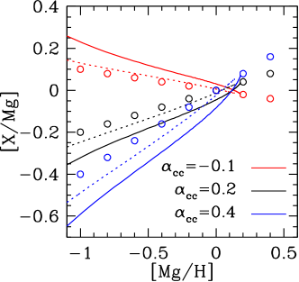
Figure 18: Tracks of $[{\rm X/Mg}]$ vs. $[{\rm Mg}/{\rm H}]$ for three different values of the yield index $\alpha_{\rm cc}=-0.1$ (red), 0.2 (black), and 0.4 (blue). Solid and dotted curves show models with exponential and linear-exponential star formation histories, respectively, all with $\tau_{\rm sfh}=6\,{\rm Gyr}$, $\tau_{*}=2\,{\rm Gyr}$, and $\eta=1.5$. Circles show the values of $[{\rm X/Mg}]$ corresponding to the yield ratio.

Figure 18 shows $[{\rm X/Mg}]-[{\rm Mg}/{\rm H}]$ tracks for three different choices of the yield index and an exponential or linear-exponential star formation history. In each case the track for a linear-exponential history is just slightly steeper than the yield metallicity-dependence. The track for an exponential history is steeper by about 0.1, with effective slopes of approximately 0.55, 0.30, $-0.20$ for $\alpha_{\rm cc}=0.4$, 0.2, and $-0.1$.

From these numerical experiments we conclude (1) that the $[{\rm X/Mg}]-[{\rm Mg}/{\rm H}]$ track for a given metallicity-dependent yield is only weakly sensitive to the chemical enrichment history, and (2) that the $[{\rm X/Mg}]-[{\rm Mg}/{\rm H}]$ track is moderately steeper than the actual metallicity dependence of the yield. The first conclusion largely explains why median sequences are nearly independent of Galactic position even for elements with metallicity-dependent yields. The second conclusion implies that the results of our 2-process model can be used as a first-cut empirical guide to the metallicity dependence of nucleosynthetic yields for the elements examined in this paper, though to test an ab initio yield model it would be better to predict median sequences directly and compare to our measurements. We have also not examined the relation of $\alpha_{\rm Ia}$ to the yield metallicity dependence for SNIa. Our median sequences run from about $[{\rm Mg}/{\rm H}]=-0.8$ to $[{\rm Mg}/{\rm H}]=0.45$, and the metallicity dependence in this regime cannot necessarily be extrapolated to much lower metallicities, where the stellar physics or nucleosynthesis physics could change in important ways.

Our inferences apply to IMF-averaged yields. For some elements, the CCSN yield is expected to depend directly on metallicity at a given supernova progenitor mass. For essentially all elements, the expected CCSN yield at a given metallicity depends strongly on the supernova progenitor mass. Even if the metallicity dependence at fixed progenitor mass is weak, the IMF-averaged yield can depend on metallicity if the IMF changes with metallicity or if the boundary between which stars explode as supernovae and which collapse directly to black holes (Pejcha & Thompson, 2015; Sukhbold et al., 2016) changes with metallicity. The success of our model in explaining the observed APOGEE sequences for even-$Z$ elements, with small inferred values of $\alpha_{\rm cc}$, provides qualitative evidence against changes in the IMF or in the mass ranges of exploding stars over the lifetime and metallicity range of the disk. However, specific scenarios for such changes should be tested directly against the observations.

5.6 Offsets of median trends

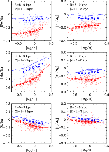
Figure 19: Offsets of median sequences at high $|Z|$ and interpretation of these offsets in terms of the 2-process model. (Top left:) Light blue and red points show [Fe/Mg] vs. [Mg/H] for ${\rm SNR}>80$ stars at $R=5-9\,{\rm kpc}$ and $|Z|=1-2\,{\rm kpc}$ in the high-[Fe/Mg] and low-[Fe/Mg] populations, respectively. Large filled circles show the median [Fe/Mg] in 0.1-dex bins of [Mg/H] for bins with at least 15 stars. Solid lines show the median trends derived from the full disk sample of ${\rm SNR}>200$ stars; at large $|Z|$, stars in the high-[Fe/Mg] population have systematically lower [Fe/Mg] than stars near the midplane, while the low-[Fe/Mg] sequence is nearly unchanged. (Top right:) Similar results for [Ni/Mg]. Open squares and connecting dashed lines show the median trend predicted by applying the 2-process model to the median [Fe/Mg] values for the high-$|Z|$ stars. (Other panels:) Similar results for Mn, Ca, Si, and O. Good agreement between the open squares and the filled circles shows that the offsets of median [X/Mg] sequences at high $|Z|$, where they are seen, can be explained by the lower median SNIa/CCSN ratio of these stars.

As noted in §3, some elements show small offsets in the median sequence for high-[Fe/Mg] stars far from the plane. Figure 19 examines this behavior more closely, comparing the median sequences of ${\rm SNR}>80$ stars with $R=5-9\,{\rm kpc}$ and $|Z|=1-2\,{\rm kpc}$ to the global median trends derived from the full disk sample of ${\rm SNR}>200$ stars. For [Fe/Mg] (top left panel), the median locus of the high-[Fe/Mg] population (blue points) is displaced downward by 0.03-0.07 dex, as seen previously in Figure 3. The low-[Fe/Mg] locus is only slightly shifted, with most points showing displacement less than 0.02 dex. The top right panel shows similar behavior for [Ni/Mg]. Open squares show the predictions of the 2-process model, with parameters inferred by fitting the full sample median sequences, applied to the median [Fe/Mg] values of this high-$|Z|$ sample. They fit the observed median sequences almost perfectly, implying that the slightly lower [Ni/Mg] values for high-$|Z|$ stars arise because these stars have a lower average SNIa/CCSN ratio even within the high-[Fe/Mg] population. The predicted (and observed) displacements are smaller than those for [Fe/Mg] because the SNIa contribution to Ni is smaller, with $R^{X}_{\rm Ia}=0.59$ instead of 1.0. Predicted (and observed) displacements are much smaller for the low-[Fe/Mg] population because the $[{\rm Fe}/{\rm Mg}]-[{\rm Mg}/{\rm H}]$ locus is itself nearly unchanged.

The middle left panel shows similar results for [Mn/Mg]. Here the 2-process model explains most of the displacement of the high-$|Z|$ median sequence, but it still slightly overpredicts the [Mn/Mg] values. The remaining panels show results for three $\alpha$-elements: Ca, Si, and O. The model fits imply that Ca has the largest SNIa contribution, so it has the largest predicted displacements of the high-$|Z|$ [X/Mg] locus, in good agreement with the data. The model also successfully predicts the smaller offset for [Si/Mg]. Even the tiny ($0.01-0.02$ dex) drop in the [O/Mg] locus accords with the small but non-zero $R^{X}_{\rm Ia}=0.07$ found for oxygen in the full sample fits.

Martig et al. (2016) find that within the high-[Fe/Mg] (low $\alpha/{\rm M}$) population, higher $\alpha/{\rm M}$ ratios correlate with older stellar ages (see their fig. 5). It is plausible that these older stars have a larger scale height because of the longer time available for dynamical heating, so that they are preferentially represented in a high-$|Z|$ sample. Relative to their mid-plane peers, the systematically smaller SNIa element fraction for these stars lowers their [Fe/Mg] ratios, and our results show that it also explains the offsets in median sequences at high $|Z|$ for other elements. The smaller the SNIa contribution to a given element, the smaller the offset.

The ability of the 2-process model to explain the systematic offsets of high-$|Z|$ sequences is a reassuring sign that it is representing the underlying physics that governs abundance ratios, not merely fitting a data set with empirical parameters. For well measured elements, we also find that the dispersion of abundance ratios relative to the star-by-star prediction of the 2-process model is smaller than the dispersion relative to the median abundance ratio of stars in the same population. For example, for ${\rm SNR}>200$ stars, the rms scatter of [Ni/Mg] ratios relative to the median sequences is 0.038 dex, while the rms scatter relative to the 2-process model predictions is 0.030 dex, a 37% reduction of variance. In physical terms, the dispersion of $[{\rm Fe}/{\rm Mg}]$ ratios at fixed [Mg/H] within a given population represents a dispersion of SNIa vs. CCSN enrichment, and other element ratios respond accordingly. Quantifying the intrinsic scatter of abundance ratios relative to the 2-process model (or median trends) requires careful assessment of the contribution of measurement errors to the observed scatter; we defer this task to a future paper.

6 Sequence fractions, MDFs, and metallicity gradients

Because the median trends we find are nearly independent of location, our full multi-element cartography can be summarized approximately by the combination of these global trends, the relative contributions of low-[Fe/Mg] and high-[Fe/Mg] populations as a function of Galactic position, and the distribution of [Mg/H] for each population as a function of Galactic position. In this section we turn our attention to the second and third of these components. While sample selection should have minimal impact on the sequences of [X/Mg] at a given [Mg/H], they can have a larger and more model-dependent effect in shaping these popuation statistics. Specifically, for a given star formation history and enrichment history, the MDF of an evolved star sample can differ from the MDF of long-lived main sequence stars because the ratio of red giants to main sequence stars changes with the age of the stellar population. Modeling the inner Galaxy population of H15, Freudenburg et al. (2017) find that the net impact on the MDF is small, but in general one should forward-model the sample selection to test a scenario of Galactic chemical enrichment. Our statistics here should be taken as those of $1<\log g<2$ stars.

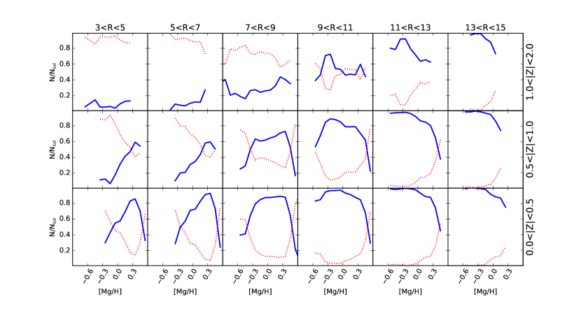
Figure 20: Fraction of stars in the low-[Fe/Mg] population (red dashed) and high-[Fe/Mg] population (blue solid) in 0.1-dex bins of [Mg/H] in the same Galactic zones used in Figs. 3-6. Low-[Fe/Mg] (“chemical thick-disk”) stars are more prevalent at high $|Z|$, small $R$, and low [Mg/H]. Data are shown only where the total number of stars per bin exceeds 30.

Figure 20 shows the fraction of low-[Fe/Mg] and high-[Fe/Mg] stars in bins of [Mg/H] in each of our 18 Galactic zones. As expected, the low-[Fe/Mg] (“chemical thick-disk”) population dominates at high-$|Z|$, small $R$, and low-[Mg/H]. For $R>5\,{\rm kpc}$ the high-[Fe/Mg] (“chemical thin-disk”) population dominates near the midplane at nearly all [Mg/H]. In the outer Galaxy, $R>11\,{\rm kpc}$, the “chemical thin-disk” population flares, and high-[Fe/Mg] stars dominate even at $|Z|=1-2\,{\rm kpc}$ (Minchev et al., 2015, 2017; Bovy, 2016; Mackereth et al., 2017). The high-[Fe/Mg] population usually dominates at super-solar [Mg/H], but our division at $[{\rm Mg/Fe}]=+0.12$ in this regime is somewhat arbitrary (see Figure 1), and the population fractions at $[{\rm Mg}/{\rm H}]>0$ are sensitive to this choice.

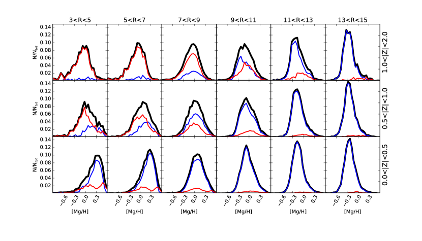
Figure 21: Distributions of [Mg/H] for all sample stars (black), low-[Fe/Mg] stars (red) and high-[Fe/Mg] stars (blue) in the same 18 Galactic zones shown in Figure 20. Distributions are computed in bins of 0.1 dex in [Mg/H], but they are plotted as curves rather than histograms for visual clarity. Near the midplane, the full sample distribution shifts from negatively skewed at small $R$ to positively skewed at large $R$, a trend that is present but weaker at high $|Z|$ (see Figure 22 below).

Figure 21 shows the [Mg/H] MDFs in each of our 18 zones, for the full sample and for the low-[Fe/Mg] and high-[Fe/Mg] populations individually. Our results are similar to those of H15, who showed distributions of [Fe/H] and [$\alpha$/H] in the same zones. Most strikingly, the midplane MDF changes shape from negatively skewed in the inner Galaxy to approximately symmetric at the solar annulus to positively skewed in the outer Galaxy. As discussed by H15, the inner Galaxy form resembles the prediction of generic one-zone evolution models, and the symmetric or positively skewed forms in the outer Galaxy can arise if radial migration from smaller $R$ is responsible for populating the high-metallicity tails. The MDF at $|Z|=1-2\,{\rm kpc}$ is roughly symmetric for $R<9\,{\rm kpc}$, though it too is positively skewed at larger $R$. For the low-[Fe/Mg] population, the change of shape is much less pronounced than for the high-[Fe/Mg] population.

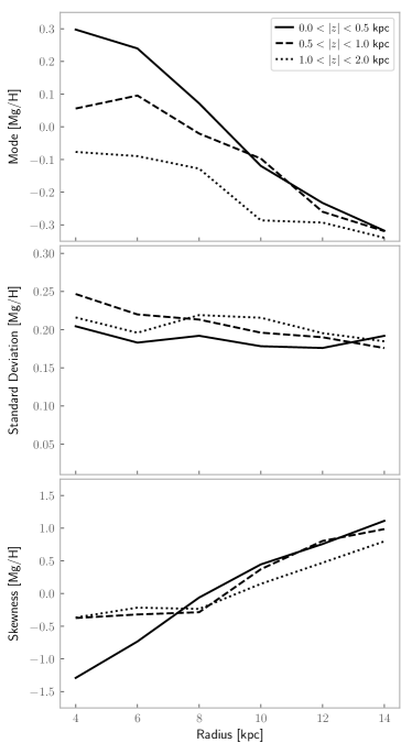
Figure 22: Mode (top panel), dispersion (middle panel), and skewness (bottom panel) of the [Mg/H] MDF as a function of Galactocentric radius, for the all-star distributions (black histograms) of Figure 21. Solid, dashed, and dotted lines show results for $|Z|/\,{\rm kpc}=0-0.5$, $0.5-1$, and $1-2$, respectively.

Figure 22 summarizes and quantifies these trends by plotting the mode, dispersion, and skewness of the [Mg/H] distribution as a function of radius, for all ${\rm SNR}>80$ stars with $[{\rm Mg}/{\rm H}]>-0.8$ in each of the three $|Z|$ bins. To reduce noise in the estimates, the mode is computed after applying kernel density estimation to create a smoothed histogram from a fine-grained [Mg/H] distribution; the dispersion and skewness are computed directly from the central moments of the stellar distribution with no binning or smoothing. Near the midplane, the modal metallicity declines from $[{\rm Mg}/{\rm H}]=+0.3$ at $R=4\,{\rm kpc}$ to $[{\rm Mg}/{\rm H}]=-0.3$ at $R=14\,{\rm kpc}$, exhibiting a roughly constant gradient of $-0.06\,{\rm dex}\,{\rm kpc}^{-1}$. Gradients are shallower at large $|Z|$ because the modal [Mg/H] is smaller in the inner Galaxy. The dispersion of the MDF is approximately constant with radius, with $\sigma_{[{\rm Mg}/{\rm H}]}\approx 0.2-0.25\,$dex for $|Z|<0.5\,{\rm kpc}$ and a slightly higher $\sigma_{[{\rm Mg}/{\rm H}]}\approx 0.25-0.3\,$dex for $|Z|=1-2\,{\rm kpc}$. The skewness plot shows the reversal of the midplane MDF shape between $R=6\,{\rm kpc}$ and $R=12\,{\rm kpc}$, with skewness changing from $-1.3$ to $+1.0$. At $|Z|=0.5-2\,{\rm kpc}$ the skewness is roughly flat at $\approx-0.4$ out to $R=8\,{\rm kpc}$, then rises steadily to $\approx+0.7$ at $R=14\,{\rm kpc}$. The values of the skewness are sensitive to the adopted lower cutoff at $[{\rm Mg}/{\rm H}]=-0.8$; including lower metallicity stars reduces the skewness values, though it does not change the qualitative trends.

Because the MDF shape changes with radius, the derived metallicity gradient depends on what statistic one uses to characterize the stellar metallicity. The mode is arguably the best choice, because it likely corresponds to the typical metallicity of stars formed in situ at each radius, while the tails of the MDF, and thus the mean of the distribution, will be more affected by radial migration of stars. Our mode gradient of $-0.06\,{\rm dex}\,{\rm kpc}^{-1}$ is comparable to that derived from Cepheid stars, approximately $-0.045\,{\rm dex}\,{\rm kpc}^{-1}$ for [Mg/H] (Genovali et al., 2015) and $-0.05\,{\rm dex}\,{\rm kpc}^{-1}$ for [Fe/H] (Luck, 2018). Gas phase oxygen abundances of HII regions yield similar estimates of radial gradients, e.g., $-0.06\,{\rm dex}\,{\rm kpc}^{-1}$ from (Rudolph et al., 2006). In principle, the median or mean metallicity gradient of the full stellar population could differ significantly from that of gas and young stars, but the metallicity gradients found in the Gaia-ESO survey by Mikolaitis et al. (2014) are at most slightly shallower, $-0.045\,{\rm dex}\,{\rm kpc}^{-1}$ for [M/H].

7 Conclusions and Prospects

Extending earlier work on “chemical cartography” of the Galactic disk with APOGEE (Hayden et al. 2014; Nidever et al. 2014; H15), we have examined the distribution of stellar abundance ratios as a function of Galactocentric radius $R$ and midplane distance $|Z|$, using 20,485 evolved stars selected from the SDSS DR14 APOGEE data set. For the elements considered in this paper, we find that the description of multi-element cartography in the Milky Way disk is approximately separable. The proportion of stars on the low-$[{\rm Fe}/{\rm Mg}]$ (“high-$\alpha$”) and high-$[{\rm Fe}/{\rm Mg}]$ (“low-$\alpha$”) sequences varies strongly with $R$, $|Z|$, and $[{\rm Mg}/{\rm H}]$. However, along each sequence the median $[{\rm X/Mg}]$ ratio depends only on $[{\rm Mg}/{\rm H}]$, with at most subtle dependence on Galactic position. The position-dependent distribution in the $[{\rm Fe}/{\rm Mg}]-[{\rm Mg}/{\rm H}]$ plane constrains the history of chemical enrichment and stellar radial migration across the disk. The nearly universal $[{\rm X/Mg}]-[{\rm Mg}/{\rm H}]$ trends provide insights on nucleosynthesis by core collapse and Type Ia supernovae.

7.1 Mg as a reference element

This separability of multi-element cartography is not evident if one simply plots $[{\rm X/Fe}]-[{\rm Fe/H}]$ distributions in different Galactic zones. The relation appears in our analysis because we adopt a pure CCSN element, Mg, as our reference, and because we separately examine trends in the low-[Fe/Mg] and high-[Fe/Mg] populations. These choices suppress misleading trends that would otherwise arise because of the changing SNIa contribution to [Fe/H]. We would obtain similar results if we used O, or a weighted mix of $\alpha$-elements, in place of Mg, but we have chosen Mg as our reference to allow simpler examination of trends within the $\alpha$-elements and straightforward comparison to other surveys (which usually measure Mg more accurately than O). Standard nucleosynthesis calculations predict that Mg is produced almost entirely by CCSN and that its IMF-averaged yield is nearly independent of metallicity (Andrews et al., 2017).

7.2 Position-dependent [Fe/Mg]-[Mg/H] distributions

For the [Fe/Mg]-[Mg/H] distributions (summarized in Figs. 20-22), our results are qualitatively similar to those of H15, who used the DR12 APOGEE data set and the [$\alpha$/M] and [M/H] ratios. Like H15 and Nidever et al. (2014) we find that the locus traced by low-[Fe/Mg] (high-[$\alpha$/M]) stars is nearly constant in all Galactic zones where we have enough stars to measure it. The fraction of low-[Fe/Mg] stars increases with $|Z|$ at fixed $R$ — the well-known “chemical thick-disk” (Bensby et al., 2003). At fixed $|Z|$, the low-[Fe/Mg] fraction is highest in the inner Galaxy and decreases outward. For the inner Galaxy, the mode of the MDF shifts to higher metallicity when moving from high $|Z|$ to the midplane, a result interpreted by Freudenburg et al. (2017) as a sign of “upside down” disk formation (Bird et al., 2013). Near the midplane, the mode of the MDF moves to lower [Mg/H] with increasing $R$, the well known radial metallicity gradient. The gradient is progressively weaker, though still present, at larger $|Z|$, as predicted in chemical evolution models where the high-$|Z|$ population is comprised of older stars (Minchev et al. 2014, see their fig. 10). The rms width of the MDF is roughly independent of position, but the shape changes from negatively skewed at small $R$ to positively skewed at large $R$, a trend that is most obvious near the midplane. H15 interpret this change of shape as a sign of stellar radial migration — in particular, the high metallicity tail of the MDF at large $R$ is comprised of stars that formed in the inner Galaxy (see, e.g., Minchev et al. 2013, fig. 3). These results provide rich and informative tests for Galactic chemical evolution models and hydrodynamic cosmological simulations. Recent simulation studies suggest that explaining the Milky Way’s observed bimodal [$\alpha$/Fe]-[Fe/H] distributions is a significant challenge (Grand et al., 2018; Mackereth et al., 2018).

7.3 Implications for nucleosynthetic yields

The approximate constancy of the median $[{\rm X/Mg}]-[{\rm Mg}/{\rm H}]$ sequences allows us to combine the full disk red giant sample and select only those stars with ${\rm SNR}>200$ spectra, yielding the distributions shown in Figs. 8-12 and the median sequences tabulated in Tables 1-6. To interpret these sequences we have developed a semi-empirical “2-process” nucleosynthesis model that assumes (a) Mg is produced purely by CCSN with a metallicity-independent IMF-averaged yield, (b) Fe is produced by CCSN and SNIa with a metallicity-independent yield, (c) other elements are the sum of a CCSN process and an SNIa process, each of which may have a power-law dependence of (X/Mg) on (Mg/H), with a relative amplitude $R^{X}_{\rm Ia}$ at solar [Mg/H]. The fits of this model to the observed median sequences are shown in Figs. 14-16. As shown in Figs. 17-18, the derived power-law slope $\alpha_{\rm cc}$ can be interpreted approximately as the implied metallicity dependence of the IMF-averaged CCSN yield in the sample range $-0.8\leq[{\rm Mg}/{\rm H}]\leq+0.4$, though the observed slope is somewhat steeper than the true yield slope by an amount that depends, slightly, on the star formation history. Constraints on the SNIa slope $\alpha_{\rm Ia}$ are often weak, and they are sensitive to the assumption of a power-law form for the CCSN dependence, so predictions of metallicity dependent SNIa yields should be tested by constructing a full forward model and allowing for uncertainties in star formation history and in the CCSN yield model. The measurement of the relative amplitude $R^{X}_{\rm Ia}$ is more robust, as it follows directly from the separation of the low-[Fe/Mg] and high-[Fe/Mg] sequences in the $[{\rm X/Mg}]-[{\rm Mg}/{\rm H}]$ diagram.

Our median sequences and 2-process fits provide a trove of quantitative constraints for supernova nucleosynthesis models. Many of the results are as expected. Among the $\alpha$-elements, O shows little SNIa contribution, while Si and Ca show progressively larger SNIa components. Among light odd-$Z$ elements, Al and K are dominated by CCSN, with a positive metallicity-dependent yield. The iron-peak elements show large SNIa contributions, with minimal metallicity dependence for the even-$Z$ elements (Cr, Fe, Ni) and strong metallicity dependence for the odd-$Z$ elements (V, Mn, Co). Of the elements considered in this paper, Mn has the largest SNIa contribution and the strongest metallicity dependence of the median sequences.

Some of our results are more surprising. The two median sequences for [S/Mg] are nearly identical, implying almost no SNIa contribution to sulfur abundances. The implied metallicity dependence of Si yields is perhaps unexpectedly strong, while that of K is perhaps unexpectedly weak. Both [Na/Mg] and [P/Mg] show large separations of the low-[Fe/Mg] and high-[Fe/Mg] sequences, implying large SNIa contributions to these elements. Our inferred SNIa contribution to Ni is substantially lower than for Fe, with $R_{\rm Ia}^{\rm Ni}=0.6$ vs. $R_{\rm Ia}^{\rm Fe}=1.0$.

7.4 Extensions and applications of the 2-process model

Our model does not allow for contributions from other nucleosynthetic sources, such as AGB stars. To the extent that the time delay distribution for AGB enrichment mimics that of SNIa enrichment, an AGB contribution could masquerade as an SNIa contribution in our model. However, the AGB contribution to the elements considered here is expected to be small. The small offset in [O/Mg] between the low-[Fe/Mg] and high-[Fe/Mg] sequences could plausibly represent an AGB contribution to oxygen, though it could also arise from model-dependent systematics in the APOGEE oxygen measurements. We have not considered more exotic scenarios in which, e.g., the stellar IMF or the mass range of CCSN progenitors or the properties of SNIa explosions change substantially with time or metallicity. The success of our simple model provides some generic evidence against such scenarios — for example, a change in the high-mass IMF would be expected to change the ratios of explosive nucleosynthesis elements (Si, S, Ca) to the hydrostatic elements O and Mg (McWilliam et al., 2013; Vincenzo et al., 2015; Carlin et al., 2018). However, any specific model must be tested for its ability to reproduce the trends observed here.

The 2-process model can be applied to individual stars as well as median sequences, predicting a star’s [X/Mg] ratios given only its [Mg/H] and [Fe/Mg] measurements. Specifically, one uses Equation (6) to infer the star’s relative SNIa enrichment contribution $A_{\rm Ia}/A_{\rm cc}$, then uses Equation (14) to predict [X/Mg]; the predicted value of [X/H] can be obtained by adding the measured [Mg/H]. In future work we will examine both the scatter in [Fe/Mg] at fixed [Mg/H] (see Bertran de Lis et al. 2016 for a recent study of [O/Fe] scatter) and correlated star-by-star deviations from the predictions of the 2-process model. The former provides constraints on the stochasticity of star formation in the galaxy, since bursts or oscillations in the star formation rate drive variations in the ratio of CCSN to SNIa enrichment (Weinberg et al. 2017; J.W. Johnson et al., in prep.). The latter could reveal signatures of additional nucleosynthesis channels beyond the IMF-averaged CCSN and SNIa processes in the current model. By removing two known strong effects on elemental abundance patterns — the ratio of CCSN to SNIa enrichment and the metallicity-dependent yields of some elements — the deviation-from-model approach may allow one to tease information from subtler observational clues.

In the longer term we aim to apply these methods to a wider range of elemental abundances and thus probe a larger set of nucleosynthesis channels. This can include APOGEE C and N abundances for main sequence or sub-giant stars that are not affected by mixing on the giant branch, the $s$-process elements Nd and Ce that are detectable in APOGEE spectra (Hasselquist et al., 2016; Cunha et al., 2017), and the many elements accessible in optical spectroscopic samples. We also plan to investigate whether bulge and halo star samples show the same supernova nucleosynthesis patterns found here for disk stars, or instead exhibit differences that could be a sign of changing IMFs or radically different yields at low metallicity.

A basic challenge of chemical evolution modeling is that abundance patterns depend on both the enrichment history of the host galaxy and on nucleosynthetic yields that are difficult to predict robustly from first principles. The approximate separability found here suggests one way to make progress, by analyzing abundance distributions in a way that isolates empirical constraints on nucleosynthesis from the broad-brush effects of galactic-scale evolution. To the extent that we can decompose star-by-star abundance patterns into sums of individual processes, the amplitudes of these processes may themselves be the best quantities to use in future chemical cartography, charting the contributions of distinct enrichment channels in different zones of the Galaxy. Precise kinematic information from Gaia also makes it feasible to change mapping variables from present-day $R$ and $|Z|$ to more intrinsically informative quantities such as guiding center radius, orbital ellipticity, and vertical action. The continuing explosive growth of Galaxy-scale multi-element abundance surveys offers bright prospects for uncovering the physical origin of the elements and the history of the Milky Way.

References

- Abolfathi et al. (2018) Abolfathi, B., Aguado, D. S., Aguilar, G., et al. 2018, ApJS, 235, 42
- Adibekyan et al. (2012) Adibekyan, V. Z., Sousa, S. G., Santos, N. C., et al. 2012, A&A, 545, A32
- Anders et al. (2014) Anders, F., Chiappini, C., Santiago, B. X., et al. 2014, A&A, 564, A115
- Andrews et al. (2017) Andrews, B. H., Weinberg, D. H., Schönrich, R., & Johnson, J. A. 2017, ApJ, 835, 224