Legendrian large cables and new phenomenon for non-uniformly thick knots

Abstract.

We define the notion of a knot type having Legendrian large cables and show that having this property implies that the knot type is not uniformly thick. Moreover, there are solid tori in this knot type that do not thicken to a solid torus with integer sloped boundary torus, and that exhibit new phenomena; specifically, they have virtually overtwisted contact structures. We then show that there exists an infinite family of ribbon knots that have Legendrian large cables. These knots fail to be uniformly thick in several ways not previously seen. We also give a general construction of ribbon knots, and show when they give similar such examples.

1. Introduction

The contact width $w\left(K\right)$ of a knot $K\subset\left(S^{3},\xi_{std}\right)$ was defined in [EH1], more or less as the largest slope of a characteristic foliation on the boundary of a solid torus representing the knot type $K$. They also defined $K$ to have the uniform thickness property if any solid torus representing the knot type $\mathcal{K}$ can be thickened to a standard neighborhood of a Legendrian representative of $K$ and $w\left(K\right)$ is equal to the maximal Thurston-Bennequin invariant $\overline{tb}\left(K\right)$ of Legendrian representatives of $K$. The usefulness of this property became evident when Etnyre-Honda showed in the same work that, if $L\subset S^{3}$ is Legendrian simple and uniformly thick, then cables of $L$ are Legendrian simple as well. Recall that a knot type is Legendrian simple if Legendrian knots in this knot type are completely determined (up to Legendrian isotopy) by their Thurston-Bennequin invariant and rotation number. They also showed that, if the cables are sufficiently negative, then they too satisfy the uniform thickness property. This allows that certain iterated cables of Legendrian simple knots are Legendrian simple, for example.

Uniform thickness has become a key hypothesis in work since then. For example, generalizing the above work on cables, in [EV], Etnyre-Vertesi showed that given a companion knot $L\subset S^{3}$ which is both Legendrian simple and uniformly thick, and a pattern $P\subset S^{1}\times D^{2}$ satisfying certain symmetry hypothesis, the knots in the satellite knot type $P_{K}$ may be understood.

Broadly, if one wants to classify Legendrian knots in a satellite knot type with companion knot $K\subset S^{3}$, and a pattern $P\subset S^{1}\times D^{2}$, then as a first step one needs to understand,

1. contact structures on the complement of a neighborhood $N$ of $K$

2. contact structures on a neighborhood $N$ of $K$

3. a classification of Legendrian knots in the knot type of the pattern $P$ in the possible contact structures on $N$.

If $K$ is uniformly thick, then $N$ can always be taken to be a standard neighborhood of $K$ with dividing curves on the boundary of slope $\overline{tb}\left(K\right)$ (i.e. maximal Thurston-Bennequin invariant of $K$), which reduces the problem to items $(1)$ and $(3)$ above. Moreover, if $K$ is Legendrian simple and uniformly thick, then $(1)$ is more or less known as well. If $K$ is not uniformly thick, then understanding satellites is much more complicated.

Similarly, uniform thickness can be useful in understanding contact surgery constructions. A typical way to obtain a new contact 3-manifold is removing a solid torus in the knot type K, and gluing in some new contact solid torus. To understand the new manifold, one needs to understand items $(1)$ and $(2)$ above, and the gluing map defining the surgery. If $K$ is uniformly thick, then $N$ can always be taken to be a standard neighborhood of $K$ with dividing curves on the boundary of slope $\overline{tb}\left(K\right)$, which simplifies $(1)$ and $(2)$ considerably.

On the other hand, there are knot types that are not uniformly thick. For such knot types, it is important to understand in what ways they can fail to be uniformly thick.

1.1. New phenomenon for non-uniformly thick knots

Given a knot type $\mathcal{K}\subset S^{3}$, the contact width of $\mathcal{K}$ is

$$w\left(\mathcal{K}\right)=\sup\left\{slope\left(\varGamma_{\partial N}\right)\mid N\;solid\;torus\;representing\;\mathcal{K}\;with\;convex\;boundary\right\}.$$

We say a solid torus represents $\mathcal{K}$ if its core is in the knot type of $\mathcal{K}$. The contact width satisfies the inequality $\overline{tb}\left(\mathcal{K}\right)\leq w\left(\mathcal{K}\right)\leq\overline{tb}\left(\mathcal{K}\right)+1$ [EH1].

A word about slope conventions. If $\mu,\lambda$ are the meridional, respectively longitudinal, curves on a torus $T$ then $\left[\lambda\right]$, $\left[\mu\right]$ form a basis for $H_{1}\left(T\right)$. A $\left(p,q\right)$ curve, or a curve of slope $\nicefrac{{q}}{{p}}$, will refer to any simple closed curve in $T$ that is in the homology class of $p\left[\lambda\right]+q\left[\mu\right]$, where $p,q\in\mathbb{Z}$ are relatively prime. This is the opposite convention to the one used in several of the main references in this paper, which were some of the first works in convex surface theory. However, it is the convention that is standard in low-dimensional topology. We caution however that, when the phrase “integer slope” is used, it would correspond to the phrase “one over integer slope” in [H, EH1, EH2] among others.

We are now in position to define uniform thickness. We say that a knot type $\mathcal{K}$ has the uniform thickness property or is uniformly thick if

1. $\overline{tb}\left(\mathcal{K}\right)=w\left(\mathcal{K}\right)$, and

2. every solid torus representing $\mathcal{K}$ can be thickened to a standard neighborhood of a maximal $tb$ representative of $\mathcal{K}$.

By a standard neighborhood of a Legendrian knot $L$, we mean a solid torus neighborhood $N$ of $L$ with convex boundary, dividing set $\varGamma_{\partial N}$ consisting of two curves, with slope $tb\left(L\right)$.

In past work, a knot type $\mathcal{K}$ can fail to have the uniform thickness property in two ways. It can have neighborhoods whose slopes are larger than $\overline{tb}$, as is the case with the unknot $U$, which has $\overline{tb}\left(U\right)=-1$ and $w\left(U\right)=0$. It can also happen that there are neighborhoods with slope strictly less than $\overline{tb}$, but that do not thicken. The first and only such examples are in [EH1] and [ELT] where it is shown that all positive torus knots $T_{p,q}$ have tori $N$ with slopes satisfying $slope\left(\varGamma_{\partial N}\right)<\overline{tb}\left(T_{p,q}\right)$ but that do not thicken. Moreover, the contact structure on all of these $N$ is universally tight.

In what follows we will denote the set of Legendrian knots, up to isotopy, in the same topological knot type as $K$ by $\mathcal{L}\left(K\right)$. We also use the convention that for a pair of relatively prime integers $p$ and $q$, the $\left(p,q\right)$ cable of $K$, that is, the knot type of a curve of slope $\nicefrac{{q}}{{p}}$ on the boundary of a torus neighborhood of $K$, is denoted by $K_{p,q}$. Notice that if $p=\pm 1$, then $K_{p,q}$ is a trivial cable in the sense that it is isotopic to the underlying knot $K$. The following theorem of Etnyre-Honda motivates us to define some new terminology.

Theorem 1.1.

(Etnyre-Honda, [EH1]) If $K\subset S^{3}$ satisfies the uniform thickness property, then for $\left|p\right|>1$ and any $L\in\mathcal{L}\left(K_{p,q}\right)$ we have that $tb\left(L\right)\leq pq$.

We generalize this result in Lemma 3.3 below. Notice that if we have a uniformly thick knot $K$ and we fix a Legendrian representative $L\in\mathcal{L}\left(K\right)$ with $tb\left(L\right)=k$, then there is an isotopy of $K$ which arranges that $L$ is a trivial cable $L=K_{1,k-1}$. But then we have that $tb\left(K_{1,k-1}\right)=tb\left(L\right)=k\nleqq k-1$, so the inequality in Theorem 1.1 is not satisfied.

Definition 1.2.

Given $\left|p\right|>1$, we will say that a Legendrian cable $L\in\mathcal{L}\left(K_{p,q}\right)$ is large if $tb\left(L\right)>pq$, and call $K_{p,q}$ Legendrian large if there exists large $L\in\mathcal{L}\left(K_{p,q}\right)$. We will then say that $K$ has Legendrian large cables, or has the Legendrian large cable (LLC) property, if any of its non-trivial cables are Legendrian large.

Notice the example above indicates that if we allowed trivial cables, the LLC property would be vacuous. Our main theorem relates the LLC property to uniform thickness.

Theorem 1.3.

If $K$ has Legendrian large cables, then there exist solid tori $V=S^{1}\times D^{2}$ representing $K$ such that $\xi\mid_{V}$ is virtually overtwisted. Moreover, $V$ cannot be thickened to a standard neighborhood of a Legendrian knot, and $K$ is not uniformly thick.

Recall that the term universally tight refers to a contact structure that is tight, and that, when lifted to the universal cover, remains tight. If the lift becomes overtwisted, then we will refer the the contact structure as virtually overtwisted.

Theorem 1.4.

Given $K$, if there exists a slope $\nicefrac{{q}}{{p}}>\overline{tb}\left(K\right)$, $\left|p\right|>1$, such that $K_{p,q}$ is Legendrian large, then $w\left(K\right)>\overline{tb}\left(K\right)$.

Question: Are there knots $K$ and slopes $\nicefrac{{q}}{{p}}<\overline{tb}\left(K\right)$ such that $K_{p,q}$ is Legendrian large?

Question: If $\xi$ is a virtually overtwisted contact structure on $S=S^{1}\times D^{2}$, for which $p$ and $q$ is there a Legendrian $\left(p,q\right)$ knot $L$ in $S$ with $tw\left(L\right)>pq$?

The knots $K^{m}$ in Figure 1.1 have $\overline{tb}\left(K^{m}\right)=-1$. Building on the work of Yasui [Y], we observe that $K_{\left(-n,1\right)}^{m}$ is Legendrian large whenever $m\leq-5$ and $1<n\leq\left\lfloor\frac{3-m}{4}\right\rfloor$. This leads to the following theorem.

\begin{overpic}[unit=1mm,scale={1}]{figure22} \put(31.0,34.0){\hbox{\pagecolor{white}\parbox{28.45274pt}{$m-1$}}} \end{overpic}

Figure 1.1. The ribbon knots $K^{m}$. There are $m-1$ right handed full twists.

Theorem 1.5.

The knots $K^{m}$ in Figure 1.1 with $m\leq-5$, are not uniformly thick in $\left(S^{3},\xi_{std}\right)$, in particular, there are solid tori $T$ representing $K^{m}$ such that $slope\left(\varGamma_{\partial T}\right)>\overline{tb}\left(K^{m}\right)$ and $\xi\mid_{T}$ is tight, but virtually overtwisted.

Remark 1.6.

Previously, there were no known examples of $\mathcal{K}$ in $\left(S^{3},\xi_{std}\right)$ with $w\left(\mathcal{K}\right)>\overline{tb}\left(\mathcal{K}\right)$, except for the unknot. These are also the first examples of solid tori in $\left(S^{3},\xi_{std}\right)$ with virtually overtwisted contact structures.

It would be interesting to know what $w\left(K^{m}\right)$ is, and what the possible non-thickenable tori in the knot type of $K^{m}$ are. We have the following partial result, following from Theorem 1.5 and its proof.

Proposition 1.7.

For $m\leq-5$, the knots $K^{m}$ in Figure 1.1 have $w\left(K^{m}\right)\geq-\frac{1}{\left\lfloor\frac{3-m}{4}\right\rfloor}$.

The origin of the examples in Theorem 1.5 come from an interesting connection between contact structures and the famous cabling conjecture first observed in [LS]. Lidman-Sivek showed that for a knot $K$ with $\overline{tb}\left(K\right)>0$, Legendrian surgery on $K$ (i.e. $\left(tb\left(K\right)-1\right)$-surgery) never yields a reducible manifold. They conjectured that this might be true with no condition on $\overline{tb}\left(K\right)$. This is equivalent to the following conjecture for any $K$ in $S^{3}$.

Conjecture 1.8.

For a Legendrian representative in the knot type $L\in\mathcal{L}\left(K_{p,q}\right)$, $tb\left(L\right)\leq pq$.

If $tb\left(L\right)>pq$ for such an $L$, then there exists $L^{\prime}$ with $tb\left(L^{\prime}\right)=pq+1$ (we can always stabilize to achieve this). Legendrian surgery on this $L^{\prime}$ would then yield a reducible manifold. In [Y], Yasui gave some interesting examples of ribbon knots which we will denote $K^{m}$, shown in Figure 1.1. In what follows, we will be concerned with integers $m<0$.

Theorem 1.9.

(Yasui, [Y]) There exist infinitely many Legendrian knots in $\left(S^{3},\xi_{std}\right)$, Figure 1.1, each of which yields a reducible 3-manifold by a Legendrian surgery in the standard tight contact structure. Furthermore, $K$ can be chosen so that the surgery coefficient is arbitrarily less than $\overline{tb}\left(K\right)$.

Yasui shows that for infinitely many pairs of integers $m,n\in\mathbb{Z}$ with $m\leq-5$, Legendrian surgery on the cables $K_{n,-1}^{m}$ yields a reducible manifold. This shows Lidman-Sivek’s conjecture to be false, and stands in contrast with Theorem 1.1 of Etnyre-Honda.

We can now easily see that $K^{m}$, Figure 1.1, does not have the uniform thickness property.

Theorem 1.10.

For integers $m\leq-5$, the ribbon knots $K^{m}$ are not uniformly thick.

The interesting features of how $K^{m}$ fails to be uniformly thick given in Theorem 1.5 require much more work.

Proof.

In [Y], Yasui shows that for integers $n\leq\frac{3-m}{4}$, the cables $K_{n,-1}^{m}$ have the property that $\overline{tb}\left(K_{n,-1}^{m}\right)=-1$. But by Theorem 1.1, if $K^{m}$ is uniformly thick, then we must have that $\overline{tb}\left(K_{n,-1}^{m}\right)\leq-n$. So for any $m\leq-5$ and any $1<n\leq\left\lfloor\frac{3-m}{4}\right\rfloor$ we arrive at a contradiction. ∎

Theorem 1.10 can be used to address the following question.

Conjecture 1.11.

If $K\subset S^{3}$ is fibered, then $K$ is uniformly thick if and only if $\xi_{K}\neq\xi_{Std}$, where $\xi_{K}$ is the contact structure induced by an open book decomposition of $K$.

Building on our above work, Hyunki Min [Min] recognized that the $K^{m}$ are counterexamples. Min showed that the $K^{m}$ are all fibered. We also know that they are slice and non-strongly-quasipositive, which implies that $\xi_{K}\neq\xi_{Std}$ by a result of Matthew Hedden [Hed]. Theorem 1.10 tells us that $K^{m}$ are not uniformly thick however, and so at least one direction of this conjecture is false. The other direction remains an interesting open question.

1.2. Ribbon knots and Legendrian large cable examples

Yasui’s examples are all ribbon knots with Legendrian large cables, and can be generalized to other families of ribbon knots. We first observe a folk result that any ribbon knot can be described in a simple way.

Theorem 1.12.

Suppose $K\subset S^{3}$ is an arbitrary ribbon knot with $n\in\mathbb{N}$ ribbon singularities. Then there is an algorithm to construct a 2-handlebody for $D^{4}$ having $n-1$ or less 1-2 handle canceling pairs such that there is an unknot $U$ in the boundary of the 1-sub-handlebody which, after attaching the 2-handles, is isotopic to $K$.

A representation of a ribbon knot $K$ as in Theorem 1.12 will be called a handlebody picture for $K$. The proof of Theorem 1.12 will be given in Section $3$. Figure 1.2 gives an example ribbon knot and its image after running the algorithm.

Theorem 1.13.

Given an arbitrary ribbon knot $K$, we can associate to it a handlebody picture. If it is possible to Legendrian realize the attaching circles of the 2-handles so that the handle attachments are Stein (i.e. framings are all $tb-1$), and also Legendrian realize $K$ so that $tb\left(K\right)=-1$, then $K$ is a Legendrian ribbon knot that bounds a Lagrangian disk in $\left(B^{4},\omega_{Std}\right)$.

\begin{overpic}[unit=1mm,scale={1}]{figure17} \put(85.0,25.0){\hbox{\pagecolor{white}\parbox{8.5359pt}{$K$}}} \put(0.0,30.0){\hbox{\pagecolor{white}\parbox{8.5359pt}{$K$}}} \end{overpic}

Figure 1.2. An example ribbon knot before running the algorithm in Theorem 1.12 (left), and after running the algorithm (right).

Proof.

Given a handlebody picture for $K$, there is an unknot $U$ in the boundary of the 1-sub-handlebody which, by hypothesis, can be realized with $tb\left(U\right)=-1$. Such an unknot bounds a Lagrangian disk in the 1-sub-handlebody. Since the 2-handles are attached disjointly from this disk, $K$ bounds a Lagrangian disk after they are attached, that is, $K$ bounds a Lagrangian disk in $\left(B^{4},\omega_{Std}\right)$. ∎

Conway-Etnyre-Tosun [CET] make use of this fact to describe when contact surgery on a knot in $\left(S^{3},\xi_{Std}\right)$ preserves symplectic fillability.

\begin{overpic}[unit=1mm,scale={1}]{figure25} \put(37.0,40.0){\hbox{\pagecolor{white}\parbox{8.5359pt}{\color[rgb]{1,0,0}$\mathcal{N}$}}} \put(37.0,8.0){\hbox{\pagecolor{white}\parbox{8.5359pt}{\color[rgb]{0.5,0,0.5}$\mathcal{S}$}}} \put(62.0,28.0){\hbox{\pagecolor{white}\parbox{8.5359pt}{\color[rgb]{0,0.5,0}$\mathcal{E}$}}} \put(-2.0,28.0){\hbox{\pagecolor{white}\parbox{8.5359pt}{\color[rgb]{0,0,1}$\mathcal{W}$}}} \put(131.0,38.0){\hbox{\pagecolor{white}\parbox{8.5359pt}{\color[rgb]{1,0,0}$\mathcal{NE}$}}} \put(63.0,38.0){\hbox{\pagecolor{white}\parbox{8.5359pt}{\color[rgb]{1,0,0}$\mathcal{NW}$}}} \put(63.0,12.0){\hbox{\pagecolor{white}\parbox{8.5359pt}{\color[rgb]{1,0,0}$\mathcal{SW}$}}} \put(131.0,12.0){\hbox{\pagecolor{white}\parbox{8.5359pt}{\color[rgb]{1,0,0}$\mathcal{SE}$}}} \put(100.0,24.0){\hbox{\pagecolor{white}\parbox{8.5359pt}{$\mathcal{T}$}}} \put(30.0,3.0){\hbox{\pagecolor{white}\parbox{8.5359pt}{$(a)$}}} \put(99.0,3.0){\hbox{\pagecolor{white}\parbox{8.5359pt}{$(b)$}}} \end{overpic}

Figure 1.3. Possible examples of knots with Legendrian large cables. The ellipses are meant to indicate a finite number of strands bundled as shown, while $\mathcal{T}$ is an arbitrary Legendrian tangle.

Corollary 1.14.

Given an arbitrary ribbon knot $K$, we can associate to it a handlebody picture. If it is possible to Legendrian realize the attaching circles of the 2-handles so that the handle attachments are Stein, Legendrian realize $K$ so that $tb\left(K\right)=-1$, and also arrange the local picture of $K$ to be as in Figure 1.3 (a), then $K$ has Legendrian large cables.

Proof.

The proof is exactly the same as the proof of Yasui’s Theorem 1.3 ([Y], pp 7-13), when there are only strands of type $\mathcal{N}$, since everything in the arguments can be done locally. The rest of the cases follow by Legendrian isotopy of Figure 1.3 (a). For example, we can change all strands of type $\mathcal{S}$ into strands of type $\mathcal{N}$ by the Legendrian isotopy shown in Figure 1.4. We can also change all strands of types $\mathcal{E}$ and $\mathcal{W}$ into strands of type $\mathcal{N}$ by even easier isotopies. ∎

\begin{overpic}[unit=1mm,scale={1}]{figure28} \put(30.0,40.0){\hbox{\pagecolor{white}\parbox{8.5359pt}{$(a)$}}} \put(99.0,40.0){\hbox{\pagecolor{white}\parbox{8.5359pt}{$(b)$}}} \put(30.0,0.0){\hbox{\pagecolor{white}\parbox{8.5359pt}{$(c)$}}} \put(99.0,0.0){\hbox{\pagecolor{white}\parbox{8.5359pt}{$(d)$}}} \end{overpic}

Figure 1.4. Shows the steps in a Legendrian isotopy to change strands of type $\mathcal{S}$ into strands of type $\mathcal{N}$.

Remark 1.15.

If the framings of the 2-handles allow stabilizations, then there are more examples. Given an arbitrary ribbon knot $K$, we can associate to it a handlebody picture. If it is possible to Legendrian realize the attaching circles of the 2-handles so that the handle attachments are Stein, Legendrian realize $K$ so that $tb\left(K\right)=-1$, arrange the local picture of $K$ to be as in Figure 1.3 (a), and arrange that there is a stabilization on each of the strands of at least one group of strands $\mathcal{NE}$, $\mathcal{NW}$, $\mathcal{SE}$, or $\mathcal{SW}$, then $K$ has Legendrian large cables. This is true since we can isotop the stabilizations to have the form of Figure 1.5 (a), Legendrian isotop the tangle $\mathcal{T}$ off to the side as shown in Figure 1.5 (b), and then apply Corollary 1.14.

\begin{overpic}[unit=1mm,scale={1}]{figure29} \put(26.0,5.0){\hbox{\pagecolor{white}\parbox{8.5359pt}{$(a)$}}} \put(89.0,5.0){\hbox{\pagecolor{white}\parbox{8.5359pt}{$(b)$}}} \put(26.0,26.0){\hbox{\pagecolor{white}\parbox{8.5359pt}{$\mathcal{T}$}}} \put(124.0,19.0){\hbox{\pagecolor{white}\parbox{8.5359pt}{$\mathcal{T}$}}} \end{overpic}

Figure 1.5. Shows a Legendrian isotopy of the tangle $\mathcal{T}$. In this example, strands of type $\mathcal{NE}$ are assumed to have stabilizations.

Acknowledgments: The author would like to express profound gratitude to his advisor John B. Etnyre for his patience, encouragement, and many helpful comments and suggestions, without which this paper would not have been possible. He would also like to extend thanks to James Conway for making him aware of Conjecture 1.11, and to Sudipta Kolay, Hyunki Min, Surena Hozoori, and Peter Lambert Cole for many useful and productive conversations.

2. Background

We will assume that the reader is familiar with Legendrian knots and basic convex surface theory. Some excellent sources for this material are [H, G, K, EH2]. We will need to understand the twisting of a contact structure along a Legendrian curve with respect to two different framings. Suppose we are given a solid torus $S\subset\left(S^{3},\xi\right)$ with convex boundary which represents the knot $K$. This just means that $S=D^{2}\times S^{1}$ and $K=\left\{pt\right\}\times S^{1}$ for some point in $int\left(D^{2}\right)$. Further suppose that we are given a Legendrian $\left(p,q\right)$ curve $L$ in $S$. Since $L$ is null-homologous in $S^{3}$, there is a well defined framing on $L$ given by any Seifert surface $\Sigma$, and measuring the twisting of $\xi$ along $L$ with respect to this framing gives us $tw\left(L;\Sigma\right)=tb\left(L\right)$, that is, the Thurston-Bennequin invariant of $L$. We can also find a boundary parallel torus $T^{2}\subset S$ containing $L$, and measure the twisting of $\xi$ along $L$ with respect to the framing coming from $T^{2}$. We will denote this twisting by $tw\left(L;\partial S\right)$. The relationship between these twistings is given by the expression [EH1]

$$tw\left(L;\partial S\right)+pq=tb\left(L\right).$$

Consider a contact structure $\xi$ on $T^{2}\times I$ with convex boundary, let $T_{1},T_{2}$ be its two torus boundary components, and assume without loss of generality that $s_{1}=slope\left(\varGamma_{T_{1}}\right)\leq slope\left(\varGamma_{T_{2}}\right)=s_{2}$, where $\varGamma_{S}$ denotes the dividing curves on a convex surface $S$. Then we will say that $\xi$ is minimally twisting if every convex, boundary parallel torus $S\subset T^{2}\times I$ has $s_{1}\leq slope\left(\varGamma_{S}\right)\leq s_{2}$. This is the same notion of minimal twisting that Honda defined in [H]. We will also need to make use of his basic slices to decompose $T^{2}\times I$ into layers. Using the same notation as above, we will call $\left(T^{2}\times I,\xi\right)$ a basic slice if

1. $\xi$ is tight, and minimally twisting,

2. $T_{i}$ are convex, and $\#\varGamma_{T_{i}}=2$,

3. $s_{i}$ form an integral basis for $\mathbb{Z}^{2}$.

Honda showed that, up to isotopy fixing the boundary, there are exactly two tight contact structures on a basic slice, distinguished by their relative Euler classes in $H^{2}\left(T^{2}\times I,\partial\left(T^{2}\times I\right);\mathbb{Z}\right)$.

The Farey tessellation, Figure 2.1, gives a convenient way to describe curves on $T^{2}$.

\begin{overpic}[unit=1mm,scale={1}]{figure23} \put(6.0,26.0){\hbox{\pagecolor{white}\parbox{8.5359pt}{\footnotesize$-1$}}} \put(57.0,26.0){\hbox{\pagecolor{white}\parbox{8.5359pt}{\footnotesize$1$}}} \put(33.0,51.0){\hbox{\pagecolor{white}\parbox{8.5359pt}{\footnotesize$0$}}} \put(32.0,2.0){\hbox{\pagecolor{white}\parbox{8.5359pt}{\footnotesize$\infty$}}} \put(21.0,49.0){\hbox{\pagecolor{white}\parbox{8.5359pt}{\footnotesize$\nicefrac{{-1}}{{3}}$}}} \put(21.0,4.0){\hbox{\pagecolor{white}\parbox{8.5359pt}{\footnotesize$-3$}}} \put(13.0,44.0){\hbox{\pagecolor{white}\parbox{8.5359pt}{\footnotesize$\nicefrac{{-1}}{{2}}$}}} \put(13.0,9.0){\hbox{\pagecolor{white}\parbox{8.5359pt}{\footnotesize$-2$}}} \put(7.0,36.0){\hbox{\pagecolor{white}\parbox{8.5359pt}{\footnotesize$\nicefrac{{-2}}{{3}}$}}} \put(7.0,17.0){\hbox{\pagecolor{white}\parbox{8.5359pt}{\footnotesize$\nicefrac{{-3}}{{2}}$}}} \put(41.0,49.0){\hbox{\pagecolor{white}\parbox{8.5359pt}{\footnotesize$\nicefrac{{1}}{{3}}$}}} \put(41.0,4.0){\hbox{\pagecolor{white}\parbox{8.5359pt}{\footnotesize$3$}}} \put(49.0,44.0){\hbox{\pagecolor{white}\parbox{8.5359pt}{\footnotesize$\nicefrac{{1}}{{2}}$}}} \put(49.0,9.0){\hbox{\pagecolor{white}\parbox{8.5359pt}{\footnotesize$2$}}} \put(55.0,36.0){\hbox{\pagecolor{white}\parbox{8.5359pt}{\footnotesize$\nicefrac{{2}}{{3}}$}}} \put(55.0,17.0){\hbox{\pagecolor{white}\parbox{8.5359pt}{\footnotesize$\nicefrac{{3}}{{2}}$}}} \end{overpic}

Figure 2.1. Farey Tessellation

To construct the eastern half of the Farey tessellation, first label the north pole by $0=\frac{0}{1}$, the south pole by $\infty=\frac{1}{0}$, and connect them by an edge (by edge, we mean a hyperbolic geodesic). Next, label the eastern most point that is midway between $0$ and $\infty$ by $1=\frac{1}{1}$, as shown in Figure 2.1. Connect $1$ by edges to $0$ and $\infty$. For rational numbers on the tessellation with the same sign, we can define an addition on the Farey tessellation by $\frac{a}{b}+\frac{c}{d}=\frac{a+c}{b+d}$, locate $\frac{a+c}{b+d}$ midway between $\frac{a}{b}$ and $\frac{c}{d}$, and connect $\frac{a+c}{b+d}$ by edges with $\frac{a}{b}$ and $\frac{c}{d}$ respectively. Thus we can fill in the rest of the positive side of the Farey tessellation by iterating this addition. Notice that, if $\frac{a}{b},\frac{c}{d}$ are assumed to be an integral basis for $\mathbb{Z}^{2}$, then both $\begin{vmatrix}a&a+c\\ b&b+d\end{vmatrix}=ad-bc=\begin{vmatrix}a&c\\ b&d\end{vmatrix}=\pm 1$ and similarly, $\begin{vmatrix}a+c&c\\ b+d&d\end{vmatrix}=\pm 1$, so any two points connected by an edge are an integral basis for $\mathbb{Z}^{2}$. Also notice that, given two positive rational numbers $\frac{a}{b}>\frac{c}{d}$, there are exactly two other points with edges to both $\frac{a}{b}$ and $\frac{c}{d}$, namely $\frac{a+c}{b+d}$ and $\frac{a-c}{b-d}$.

To construct the western (negative) half of the Farey tessellation, first relabel the north pole by $0=\frac{0}{-1}$. Next, label the western most point that is midway between $0$ and $\infty$ by $-1=\frac{1}{-1}$, as shown in Figure 2.1. Connect $-1$ by edges to $0$ and $\infty$. Now using the same addition we defined above, we can iteratively build up the negative side of our Farey tessellation. Notice that the only point which was labeled twice was the north pole, which is now given by $\frac{0}{\pm 1}$.

For any two points $p_{1}$ and $p_{2}$ on the Farey tessellation, we define the interval $\left[p_{1},p_{2}\right]$ to be the set of all points encountered starting from $p_{1}$ and moving clockwise around the tessellation until reaching $p_{2}$. Given a clockwise sequence of three points connected by edges $p_{1}$, $p_{2}$ and $p_{3}$ on the Farey tessellation, we say that a jump from $p_{2}$ to $p_{3}$ is half maximal if $p_{3}$ is the half way point of the maximum possible clockwise jump one could make in the interval $\left(p_{2},p_{1}\right)$. We will consider only clockwise paths in the Farey tessellation, where a path is a sequence of jumps along edges. We call a path between two points $s_{1},s_{2}\in\mathbb{Q}$ a continued fraction block if, after the first jump, every jump is half maximal. Notice that, by construction, a path that is a continued fraction block cannot be shortened. We will also need to consider decorated paths (i.e. paths for which each jump gets a “$+$” or “$-$”). We can define an equivalence relation “$\sim$” on decorated paths in the Farey tessellation which says that any two paths with the same endpoints and which differ only by shuffling of signs within continued fraction blocks are in the same class. The following result, due to Honda [H], and in a different terminology Giroux [G], describes a relationship between contact structures on $T^{2}\times I$ and minimal decorated paths in the Farey tessellation. Given a manifold $M$ and a multicurve $\varGamma$ in $\partial M$, let $Tight\left(M,\varGamma\right)$ denote the set of isotopy classes of tight contact structures on $M$ with convex boundary, such that $\varGamma$ is a set of dividing curves for $\partial M$. Similarly, given $T^{2}\times I$ with boundary $T_{1}\sqcup T_{2}$, and two multicurves $\varGamma_{i}$ on $T_{i}$, let $Tight\left(T^{2}\times I,T_{1}\cup T_{2}\right)$ denote the set of tight, minimally twisting contact structures on $T^{2}\times I$ with convex boundary, such that $\varGamma_{i}$ is a set of dividing curves for $T_{i}$.

Theorem 2.1.

(Honda, [H]) Given $T^{2}\times I$ with boundary $T_{1}\sqcup T_{2}$, and two multicurves $\varGamma_{i}$ on $T_{i}$ with $\#\varGamma_{i}=2$ such that $s_{1}=slope\left(\varGamma_{1}\right)\leq slope\left(\varGamma_{2}\right)=s_{2}$, then

$$Tight\left(T^{2}\times I,\varGamma_{1}\cup\varGamma_{2}\right)\nicefrac{{\longleftrightarrow\begin{Bmatrix}minimal\;decorated\;paths\\ from\;s_{1}to\;s_{2}\end{Bmatrix}}}{{\sim}}.$$

Given $T^{2}\times I$ with a two component multicurve on each of its two torus boundary components, and with boundary slopes $s_{1},s_{2}\in\mathbb{Q}$, then any decorated path starting from $s_{1}$ and ending at $s_{2}$ describes a contact structure on $T^{2}\times I$. Each jump in the path describes a basic slice, and therefore has two possible contact structures distinguished by the relative Euler class. We then get $T^{2}\times I$ by concatenating together these basic slices. For more details, see [H]. It follows from Theorem 2.1 that within any continued fraction block, shuffling the signs of the jumps results in isotopic contact structures.

Suppose we have a decorated path which can be shortened, see Figure 2.2. It follows from Honda’s gluing theorem that if the two jumps which are being combined into a single jump have different signs, then the contact structure on $T^{2}\times I$ described by this path is overtwisted. If the signs agree, then the contact structure will be tight. For this reason, we say that a shortening is consistent if the signs of the smaller jumps agree, and make the following theorem owing to Honda.

Theorem 2.2.

Given a decorated path in the Farey tessellation from $s_{1}$ to $s_{2}$, the contact structure on $T^{2}\times I$ with convex boundary $T_{1}\sqcup T_{2}$, $\#\varGamma_{T_{i}}=2$, and $s_{1}=slope\left(\varGamma_{T_{1}}\right),\;slope\left(\varGamma_{T_{2}}\right)=s_{2}$ described by this path is tight if and only if every shortening is consistent.

To classify the tight contact structures on solid tori, we will consider a slightly different type of path. Let a truncated path be a decorated path, as defined above, with the sign of the first jump omitted from consideration. In other words, the first jump is not decorated. Suppose we have $S^{1}\times D^{2}$ with a two component multicurve on its torus boundary, and with boundary slope $s_{2}\in\mathbb{Q}$. If the meridian of $\partial\left(S^{1}\times D^{2}\right)$ has slope $s_{1}\in\mathbb{Q}$, then we have the following classification. Given $S^{1}\times D^{2}$ with boundary $T$, and a multicurve $\varGamma$ on $T$, let $Tight\left(S^{1}\times D^{2},\varGamma\right)$ denote the set of isotopy classes of tight, minimally twisting contact structures on $S^{1}\times D^{2}$ with convex boundary, such that $\varGamma$ is a set of dividing curves for $T$.

\begin{overpic}[unit=1mm,scale={1}]{figure24} \put(24.0,27.0){\hbox{\pagecolor{white}\parbox{2.84544pt}{\color[rgb]{1,0,0}\tiny$+$}}} \put(30.0,31.0){\hbox{\pagecolor{white}\parbox{2.84544pt}{\color[rgb]{1,0,0}\tiny$+$}}} \put(27.0,24.0){\hbox{\pagecolor{white}\parbox{2.84544pt}{\color[rgb]{1,0,0}\tiny$+$}}} \put(65.0,27.0){\hbox{\pagecolor{white}\parbox{2.84544pt}{\color[rgb]{1,0,0}\tiny$+$}}} \put(69.0,24.0){\hbox{\pagecolor{white}\parbox{2.84544pt}{\color[rgb]{1,0,0}\tiny$-$}}} \end{overpic}

Figure 2.2. On the left, a consistent shortening, while on the right a shortening which is not consistent.

Theorem 2.3.

(Honda, [H]) Given $S^{1}\times D^{2}$with boundary $T$, and a multicurve $\varGamma$ on $T$ with $\#\varGamma=2$ such that $s_{2}=slope\left(\varGamma\right)$, and $s_{1}=slope\left(\mu\right)$, where $\mu$ is a meridional curve for $T$, then

$$Tight\left(S^{1}\times D^{2},\varGamma\right)\nicefrac{{\longleftrightarrow\begin{Bmatrix}minimal\;truncated\;paths\\ from\;s_{1}\;to\;s_{2}\end{Bmatrix}}}{{\sim}}.$$

Theorem 2.4.

(Honda, [H]) (1) Given $T^{2}\times I$ with boundary $T_{1}\sqcup T_{2}$, and two multicurves $\varGamma_{i}$ on $T_{i}$ with $\#\varGamma_{i}=2$ such that $s_{1}=slope\left(\varGamma_{1}\right)\leq slope\left(\varGamma_{2}\right)=s_{2}$, there are exactly two tight contact structures on $T^{2}\times I$, and these contact structures are universally tight. The paths describing these two structures are the same, one decorated entirely by “$+$”, and the other decorated entirely by “$-$”.

(2) Given $S^{1}\times D^{2}$with boundary $T$, and a multicurve $\varGamma$ on $T$ with $\#\varGamma=2$ such that $s_{2}=slope\left(\varGamma\right)$, and $s_{1}=slope\left(\mu\right)$, where $\mu$ is a meridional curve for $T$, then, if $s_{1}\cdot s_{2}\neq\pm 1$, there are exactly two tight contact structures on $S^{1}\times D^{2}$, and these contact structure is universally tight. The paths describing these two structures are the same, one decorated entirely by “$+$”, and the other decorated entirely by “$-$”. If $s_{1}\cdot s_{2}=\pm 1$, then there exists a unique tight contact structure on $S^{1}\times D^{2}$, and this contact structure is universally tight.

It follows from Theorem 2.4 that if we have a path with a mixture of signs, then the contact structure described by this path on either $T^{2}\times I$, or on $S^{1}\times D^{2}$, must be virtually overtwisted.

3. Cables in Solid Tori

In this section, we will give the proof of Theorems 1.3,  1.4, and  1.5. We would like to record and make use of the following result.

Theorem 3.1.

(Etnyre-Honda, [EH1]) Any cable in a standard neighborhood of a Legendrian knot can be put on a convex torus.

Proposition 3.2.

If $\xi$ is a universally tight contact structure on a solid torus $S$ with convex boundary, then any Legendrian $\left(p,q\right)$ knot $L\subset S$ has $tw\left(L;\partial S\right)\leq 0$.

We delay the proof of Proposition 3.2 to the end of this section, but use it here to give proofs of our main theorems stated in the introduction.

Proof of Theorem 1.3

If $K$ has Legendrian large cables, then there exists $L\in\mathcal{L}\left(K_{p,q}\right)$ such that $tb\left(L\right)>pq$. Take a solid torus $S$ representing $K$ and containing $L$ as a $\left(p,q\right)$ curve. Perturb $S$ to have convex boundary. By hypothesis $tw\left(L;\partial S\right)>0$, so by Proposition 3.2, $\left.\xi\right|_{S}$ must be virtually overtwisted. Suppose that it were possible to thicken $S$ to a standard neighborhood $\widetilde{S}$ of $K$. Then $slope\left(\varGamma_{\partial\widetilde{S}}\right)\in\mathbb{Z}$ which implies by a result of Kanda [K], that $\left.\xi\right|_{\widetilde{S}}$ is the unique tight contact structure on $\widetilde{S}$, and moreover that $\left.\xi\right|_{\widetilde{S}}$ is universally tight. But this is a contradiction since $S\subset\widetilde{S}$ and $\left.\xi\right|_{S}$ is virtually overtwisted, so no such thickening exists. If $K$ were uniformly thick, then any neighborhood of $K$ would be thickenable to a $slope\left(\overline{tb}(K)\right)$ standard neighborhood of $K$, which we have just seen is not possible. □

Proof of Theorem 1.4

By assumption, there exists $L\in\mathcal{L}\left(K_{p,q}\right)$ such that $tb\left(L\right)>pq$. Stabilize $L$ to obtain $\widetilde{L}$ such that $tb\left(\widetilde{L}\right)=pq$. There is a solid torus $S$ representing $K$ for which $\widetilde{L}\subset\partial S$, and as discussed at beginning of Section $2$, we see that $tw\left(\widetilde{L};\partial S\right)=0$. We can therefore $C^{0}$ perturb a collar neighborhood $N$ of $\widetilde{L}$ in $\partial S$ to be convex, and then $C^{\infty}$ perturb $\partial S\setminus N$ to obtain a solid torus $\widetilde{S}$ representing $K$ with convex boundary. Since $tw\left(\widetilde{L};\partial\widetilde{S}\right)=0$, and since $slope\left(\widetilde{L}\right)=\frac{q}{p}$, we must have that $slope\left(\varGamma_{\partial\widetilde{S}}\right)=\frac{q}{p}$, owing to the fact that $tw\left(\widetilde{L};\widetilde{S}\right)=-\frac{1}{2}\left|\widetilde{L}\bullet\varGamma_{\partial\widetilde{S}}\right|$ where $C_{1}\bullet C_{2}$ denotes the geometric intersection number of two curves on a torus. But $\frac{q}{p}>\overline{tb}(K)$ by assumption, so $w\left(K\right)>\overline{tb}(K)$. □

Proof of Theorem 1.5

In [Y], Yasui shows that for integers $n\leq\frac{3-m}{4}$, the cables $K_{n,-1}^{m}$ have the property that $\overline{tb}\left(K_{n,-1}^{m}\right)=-1$. So for any $m\leq-5$ and any $1<n\leq\left\lfloor\frac{3-m}{4}\right\rfloor$ we see that $K^{m}$ has Legendrian large cables $L\in\mathcal{L}\left(K_{n,-1}^{m}\right)$. Then by Theorem 1.3 $K^{m}$ is not uniformly thick and has virtually overtwisted neighborhoods, and by Theorem 1.4 we have that $w\left(K^{m}\right)>\overline{tb}(K^{m})$ □

Proof of Proposition 1.7

The slope of the cable $K_{n,-1}^{m}$ is $slope\left(K_{n,-1}^{m}\right)=-\frac{1}{n}$. Whenever $n\leq\frac{3-m}{4}$, we know there exist $L\in\mathcal{L}\left(K_{n,-1}^{m}\right)$ which are Legendrian large. Stabilize $L$ to obtain $\widetilde{L}$ such that $tb\left(\widetilde{L}\right)=-n$. There is a solid torus $S$ representing $K^{m}$ for which $\widetilde{L}\subset\partial S$, and we have seen that $tw\left(\widetilde{L};\partial S\right)=0$. Using the strategy of the proof of Theorem 1.4, we can $C^{0}$ perturb a collar neighborhood $N$ of $\widetilde{L}$ in $\partial S$ to be convex, and then $C^{\infty}$ perturb $\partial S\setminus N$ to obtain a solid torus $\widetilde{S}$ representing $K^{m}$ with convex boundary. Since $tw\left(\widetilde{L};\partial\widetilde{S}\right)=0$, and since $slope\left(\widetilde{L}\right)=-\frac{1}{n}$, we must have that $slope\left(\varGamma_{\partial\widetilde{S}}\right)=-\frac{1}{n}$, and therefore that $w\left(K^{m}\right)\geq-\frac{1}{n}$. □

Now we will give a series of results leading to the proof of Proposition 3.2.

Lemma 3.3.

Let $S$ be a solid torus with convex boundary, $\left|\varGamma_{\partial S}\right|=2$, and $slope\left(\varGamma_{\partial S}\right)\in\mathbb{Z}$ with its unique tight contact structure $\xi$, then any Legendrian $\left(p,q\right)$ knot $L\subset S$ has $tw\left(L;\partial S\right)\leq 0$.

Proof.

Notice that this follows immediately from Theorem 3.1, since $S$ is a standard neighborhood, and any Legendrian curve $L$ on a convex torus $T$ must have $tw\left(L;T\right)=tw\left(L;\partial S\right)\leq 0$. Alternatively, we can reason in the following way. Recall that Kanda [K] showed that any solid torus with integer slope and two dividing curves has a unique tight contact structure. Suppose that $S$ is a solid torus with convex boundary, $\left|\varGamma_{\partial S}\right|=2$, and $slope\left(\varGamma_{\partial S}\right)=k\in\mathbb{Z}$ with its unique tight contact structure $\xi$, and that $L\subset S$ is a Legendrian $\left(p,q\right)$ knot. Then $S$ is a standard neighborhood of a Legendrian core curve $K$. Any two standard neighborhoods are contactomorphic, so we can find a neighborhood $N\subset\left(S^{3},\xi_{std}\right)$ of a Legendrian unknot $U\subset S^{3}$ with $tb\left(U\right)=-1$, and a contactomorphism $\varphi:S\rightarrow N$ which sends $\varphi\left(K\right)=U$. This contactomorphism sends torus knots to torus knots, so our $\left(p,q\right)$ knot $L$ is mapped to a $\left(p,q-p\left(k+1\right)\right)$ knot $\varphi\left(L\right)$ as one can easily check. But now $\varphi\left(L\right)$ is a torus knot in $\left(S^{3},\xi_{std}\right)$, and Etnyre and Honda have shown [EH2] that $tb\left(\varphi\left(L\right)\right)\leq p\left(q-p\left(k+1\right)\right)$. But we understand how to switch between the Seifert framing and the framing coming from the torus $\partial N$, that is, $tw\left(\varphi\left(L\right);\partial N\right)=tb\left(\varphi\left(L\right)\right)-p\left(q-\left(k+1\right)\right)\leq 0$. This implies that $tw\left(L;\partial S\right)\leq 0$, since $N$ and $S$ are contactomorphic. ∎

We can strengthen Lemma 3.3 slightly by dropping the assumption that $\left|\varGamma\right|=2$.

Lemma 3.4.

Let $S$ be a solid torus with convex boundary, and $slope\left(\varGamma_{\partial S}\right)\in\mathbb{Z}$ with any tight contact structure $\xi$, then any Legendrian $\left(p,q\right)$ knot $L\subset S$ has $tw\left(L;\partial S\right)\leq 0$.

Proof.

We will show that $\left(S,\xi\right)$ will embed in a tight contact structure $\left(\widetilde{S},\widetilde{\xi}\right)$ that satisfies the hypothesis of Lemma 3.3, and therefore show that $tw\left(L;\partial S\right)\leq 0$. To this end, we note that we can assume $slope\left(\varGamma_{\partial S}\right)=0$ by applying a diffeomorphism to $S$. Recall [H], that $\xi$ is completely determined by the dividing set $\varGamma_{D}$ on a meridional disk $D$ of $S$. We will build a model situation for $S$ in which we can construct $\left(\widetilde{S},\widetilde{\xi}\right)$. Since $\left|\varGamma_{\partial S}\right|>2$ we see that $\left|\varGamma_{D}\right|>1$. Suppose that we have a convex disk $D$ with an arbitrary collection of dividing curves $\varGamma$, as in Figure 3.1.

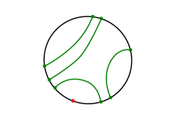
Figure 3.1. Arbitrary disk with arcs.

Let $v$ be a vector field on $D$ that guides the characteristic foliation. We can label the regions in $D\setminus\varGamma$ as either $\varSigma^{+}$ or $\varSigma^{-}$ so that no adjacent pair share the same label. There exists an area form $\omega$ on $D$ which satisfies that $\pm div_{\omega}v>0$ on $\varSigma^{\pm}$. Assign a 1-form $\lambda=\iota_{v}\omega$, then we know from Giroux [G] that there exists a function $u:D\rightarrow\mathbb{R}$ such that $udt+\lambda$ gives rise to a contact structure $\xi$ on $D\times\mathbb{R}$ that is invariant in the $\mathbb{R}$ direction. Moreover, we know from a theorem of Giroux that $\xi$ is tight, since there are no homotopically trivial dividing curves. This invariance means that we can mod out by $\mathbb{Z}$ to obtain a tight contact structure on a solid torus $\nicefrac{{D\times\mathbb{R}}}{{\mathbb{Z}}}=D\times S^{1}$. The solid torus and contact structure we obtain in this way are contactomorphic to our original $\left(S,\xi\right)$, that is, there exists $v,\omega$ and $u:D\rightarrow\mathbb{R}$ for which this construction exactly reproduces $\left(S,\xi\right)$.

Now suppose that the number of properly embedded arcs is greater than $1$. We would now like to reduce the number of dividing curves by taking a larger disk containing our original $D$. So we attach an annulus to $D$ to obtain $D_{ext}=D\cup_{\varphi}\left(S^{1}\times\left[0,1\right]\right)$ where $\varphi:S^{1}\times\left\{0\right\}\rightarrow\partial D$ is the gluing map. Denote the endpoints of the properly embedded arcs as $\left\{x_{1},\ldots,x_{2k}\right\}$. Notice that if we fix a point on $p\in\partial D$ and move counterclockwise from $p$ along $\partial D$, then it must happen that we encounter an $x_{i}$ followed by an $x_{i+1}$ which are not endpoints of the same curve. If this were not so, then there could only be one curve, which we have supposed not to be the case. Without loss of generality, assume that these two points are $x_{1}$ and $x_{2}$. Now connect these points by an arc in $S^{1}\times\left[0,1\right]$. Form arcs from the remaining points $\left\{x_{3},\ldots,x_{2k}\right\}$ to $\partial D_{ext}$ by using $\left\{x_{i}\right\}\times\left[0,1\right]$, as in Figure 3.2. Notice that $D_{ext}$ has one fewer embedded arcs than $D$. So we can iterate this procedure to obtain a disk $\widetilde{D}\supset D$ which has only $1$ properly embedded arc. Call this arc $\widetilde{\varGamma}$. Notice that we can arrange the gluing map $\varphi$ to be smooth and such that the extension of $\varGamma$ to $\widetilde{\varGamma}$ is smooth. We can also smoothly extend $\omega$ and $v$ to $\widetilde{D}$ so that the singular foliation on $\widetilde{D}$ guided by $v$ has $\widetilde{\varGamma}$ as a dividing curve. We can now build, just as we did above, a contact structure $\widetilde{\xi}$ on $\widetilde{D}\times S^{1}=\widetilde{S}$ having $\widetilde{D}$ as a convex meridional disk, with convex boundary. Since $\left|\varGamma_{\widetilde{D}}\right|=1$ we see that $tb\left(\partial\widetilde{D}\right)=-1$, which in turn implies that $\left|\varGamma_{\partial\widetilde{S}}\right|=2$. Notice that $\left.\widetilde{\xi}\right|_{S}=\xi$. Also notice that, by construction, the method of reducing the number of dividing curves on $\partial S$ yields $slope\left(\varGamma\right)=slope\left(\widetilde{\varGamma}\right)$. Now by Lemma 3.3, any Legendrian $\left(p,q\right)$ knot $L\subset S$ has $tw\left(L;\partial S\right)\leq 0$.

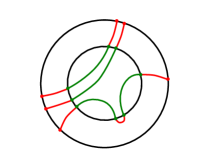
Figure 3.2. An annulus has been attached, and the number of curves has been reduced by one.

∎

Lemma 3.5.

If $\xi$ is a universally tight contact structure on a solid torus $S$ with convex boundary and $\left|\varGamma_{\partial S}\right|=2$, then any Legendrian $\left(p,q\right)$ knot $L\subset S$ has $tw\left(L;\partial S\right)\leq 0$.

Proof.

By a diffeomorphism of $S$, we can assume that $slope\left(\varGamma_{\partial S}\right)=-\nicefrac{{r}}{{s}}$ where $-\infty\leq-\nicefrac{{r}}{{s}}\leq-1$, and that the meridional slope is $-\infty$. Let $n=\left\lceil\nicefrac{{r}}{{s}}\right\rceil$. Then since $\xi$ is universally tight, we know that any path in the Farey tessellation, describing our contact structure has the property that each jump must be decorated with the same sign by Theorem 2.1. A portion of the Farey tessellation shows this in Figure 3.3. We can obtain a larger solid torus $\widetilde{S}\supset S$, convex, two dividing curves, and with $slope\left(\varGamma_{\partial\widetilde{S}}\right)=-n+1$ in the following way. Take a shortest path in the Farey tessellation from $-\nicefrac{{r}}{{s}}$ to $-n+1$, and decorate each jump with the sign which appears in the description of the contact structure on $S$. This describes a contact structure on $T^{2}\times I$ which extends $S$ to $\widetilde{S}$, and since the signs are all the same we know that $\widetilde{S}$ is tight by Theorem 2.2. Moreover, we see that $\widetilde{S}$ has integer slope giving it a unique tight contact structure. Now we have that $tw(K;\partial S)\leq 0$ by Lemma 3.3.

\begin{overpic}[unit=1mm,scale={1}]{figure21} \put(29.0,8.0){\hbox{\pagecolor{white}\parbox{2.84544pt}{$-n$}}} \put(3.0,29.0){\hbox{\pagecolor{white}\parbox{34.14322pt}{$-n+1$}}} \put(15.0,18.0){\hbox{\pagecolor{white}\parbox{2.84544pt}{$-\nicefrac{{r}}{{s}}$}}} \end{overpic}

Figure 3.3. Farey tessellation picture describing the contact structure on our solid torus. The original solid torus, $S$, is shown in blue, while the red indicates the $T^{2}\times I$ which is glued on to obtain the larger solid torus $\widetilde{S}$.

∎

Remark 3.6.

In the above proof, we are able to thicken $S$ to a larger solid torus $\widetilde{S}\supseteq S$ with $slope\left(\varGamma_{\partial\widetilde{S}}\right)=-n+1$ because we are thinking of $S=S^{1}\times D^{2}$ abstractly as a contact 3-manifold with convex boundary, and not embedded in any particular contact manifold. There is a shortest path in the standard Farey tessellation picture from any negative rational $-\nicefrac{{r}}{{s}}$ to $-n+1$ which describes our contact structure. We are not claiming that if $S$ is a solid torus representing a knot $K\subseteq S^{3}$ it must always be thickenable in $S^{3}$, for example, Etnyre, LaFountain, and Tosun have given examples of non-thickenable tori in [ELT].

Proposition 3.2 strengthens Lemma 3.5 slightly by dropping the assumption that $\left|\varGamma\right|=2$.

Proof of Proposition 3.2

Suppose we are given a solid torus $S$ with convex boundary, a universally tight contact structure $\xi$, and we have a Legendrian $\left(p,q\right)$ knot $L$ in $S$. Again, by a diffeomorphism of $S$, we can assume that $slope\left(\varGamma_{\partial S}\right)=-\nicefrac{{r}}{{s}}$ where $-\infty\leq-\nicefrac{{r}}{{s}}\leq-1$, that the meridional slope is $-\infty$. Let $n=\left\lceil\nicefrac{{r}}{{s}}\right\rceil$. If $\left|\varGamma_{\partial S}\right|=2k>2$, then we can attach a bypass to $\partial S$ along a Legendrian ruling curve to obtain a smaller solid torus $S^{\prime}\subset S$ which has $slope\left(\varGamma_{\partial S^{\prime}}\right)=-\nicefrac{{r}}{{s}}$ and $\left|\varGamma_{\partial S^{\prime}}\right|=2k-2$. We can repeat this procedure until we have a solid torus $\widetilde{S}\subset S$ which has $slope\left(\varGamma_{\partial\widetilde{S}}\right)=-\nicefrac{{r}}{{s}}$ and $\left|\varGamma_{\partial\widetilde{S}}\right|=2$. Notice that the contact structure on $\widetilde{S}$ is just $\left.\xi\right|_{\widetilde{S}}$. If we look at a meridional disk $D\subset S$, we know that along $\partial D$ there are $2sk$ intersection points with $\varGamma_{\partial S}$, however there exists a slope $\gamma$ for which, curves on $\partial S$ of slope $\gamma$ have exactly $2k$ intersection points with $\varGamma_{\partial S}$. For convenience, change coordinates on $S$ so that $slope\left(\gamma\right)\mapsto-\infty$ and $slope\left(\varGamma_{\partial S}\right)\mapsto 0$. Notice that we have a $T^{2}\times I$ layer $X=S\setminus\widetilde{S}$, and we can find a convex annulus $A$ in $X$ with Legendrian boundary of slope $\gamma$. We would like to show that the contact structure on $X$ is completely determined by the dividing curves on $A$. Since $\left|\varGamma_{\partial\widetilde{S}}\right|=2$, $\left|\varGamma_{\partial S}\right|=2k$, and $slope\left(\varGamma_{\partial\widetilde{S}}\right)=slope\left(\varGamma_{\partial S}\right)=0$, we know that the dividing curves on $A$ must have the form shown in Figure 3.4 (b) by the green arcs.

\begin{overpic}[unit=1mm,scale={1}]{figure26} \put(56.0,38.0){\hbox{\pagecolor{white}\parbox{2.84544pt}{$S$}}} \put(50.0,23.0){\hbox{\pagecolor{white}\parbox{2.84544pt}{$A$}}} \put(111.0,23.0){\hbox{\pagecolor{white}\parbox{2.84544pt}{$A$}}} \put(30.0,1.0){\hbox{\pagecolor{white}\parbox{2.84544pt}{$(a)$}}} \put(99.0,1.0){\hbox{\pagecolor{white}\parbox{39.83368pt}{$(b)$}}} \put(10.0,36.0){\hbox{\pagecolor{white}\parbox{2.84544pt}{\color[rgb]{1,0,0}$B$}}} \end{overpic}

Figure 3.4. On the left, $X=T^{2}\times I$, and on the right, the annulus $A$ and its dividing curves.

We know from Giroux [G] that the contact structure on a neighborhood of $A$ is determined by its dividing curves. If we cut $X$ along $A$, and round corners, we obtain a solid torus $Y$ with convex boundary. Using the edge rounding lemma [H], it is easy to see that $\left|\varGamma_{\partial Y}\right|=2$ and $slope\left(\varGamma_{\partial Y}\right)=-1$. Notice in Figure 3.4 (a) that we have a meridional disk $B$ of $Y$ which we have just seen has $tw\left(\partial B\right)=-1$, and which we can perturb to be convex. There is a unique choice of dividing curves on such a disk. Finally, if we cut $Y$ along $B$ and round corners, we obtain a $B^{3}$ with convex boundary, which has a unique tight contact structure from work of Eliashberg [Eliash]. So we have seen that the contact structure of $X$ is determined solely by the dividing curves on $A$.

Let $v$ be a vector field on $A$ that guides the characteristic foliation. We can label the regions in $A\setminus\varGamma$ as either $\varSigma^{+}$ or $\varSigma^{-}$ so that no adjacent pair share the same label. There exists an area form $\omega$ on $A$ which satisfies that $\pm div_{\omega}v>0$ on $\varSigma^{\pm}$. Assign a 1-form $\lambda=\iota_{v}\omega$, then we know from Giroux [G] that there exists a function $u:A\rightarrow\mathbb{R}$ such that $udt+\lambda$ gives rise to a contact structure $\xi$ on $A\times\mathbb{R}$ that is invariant in the $\mathbb{R}$ direction. Moreover, we know from a theorem of Giroux that $\xi$ is tight, since there are no homotopically trivial dividing curves. This invariance means that we can mod out by $\mathbb{Z}$ to obtain a tight contact structure on $\nicefrac{{A\times\mathbb{R}}}{{\mathbb{Z}}}=T^{2}\times I$. The $T^{2}\times I$ layer and contact structure we obtain in this way are contactomorphic to our original $\left(X,\xi\right)$, that is, there exists $v,\omega$ and $u:A\rightarrow\mathbb{R}$ for which this construction exactly reproduces $\left(X,\xi\right)$.

Now observe that we can smoothly extend $A$, abstractly, by an annulus $\widehat{A}$ causing the number of dividing curves to be reduced to $2$, just as we did with the disk in the proof of Lemma 3.4, see Figure 3.5.

\begin{overpic}[unit=1mm,scale={1}]{figure27} \put(42.0,23.0){\hbox{\pagecolor{white}\parbox{2.84544pt}{\footnotesize$A$}}} \put(111.0,23.0){\hbox{\pagecolor{white}\parbox{2.84544pt}{\footnotesize$A$}}} \put(119.0,23.0){\hbox{\pagecolor{white}\parbox{2.84544pt}{\footnotesize$\widehat{A}$}}} \end{overpic}

Figure 3.5. Reducing the number of dividing curves on $A$ by extending with an annulus $\widehat{A}$

We can arrange that the extension of $\varGamma_{A}$ to $\varGamma_{A\cup\widehat{A}}$ is smooth, and we can also smoothly extend $\omega$ and $v$ to a neighborhood of $\widehat{A}$ so that the singular foliation on $\widehat{A}$ guided by $v$ has $\varGamma_{A\cup\widehat{A}}$ as a set of dividing curves. We can now build, just as we did above, a contact structure $\widehat{\xi}$ on $\left(A\cup\widehat{A}\right)\times S^{1}=\widehat{X}$ with convex boundary. Since $\left|\varGamma_{A\cup\widehat{A}}\right|=2$ we see that $tb\left(\partial\widehat{A}\cap\partial\widehat{X}\right)=-1$, which implies that $\left|\varGamma_{\partial\widehat{X}}\right|=2$. Notice that $\left.\widehat{\xi}\right|_{X}=\xi$. Also notice that, by construction, the method of reducing the number of dividing curves on $\partial X$ yields $slope\left(\varGamma_{\partial X}\right)=slope\left(\varGamma_{\partial\widehat{X}}\right)$. But now we have a minimally twisting $T^{2}\times I$ layer $\widehat{X}$ whose boundary tori each have two dividing curves with slope $0$. Honda showed [H] that there are an integers worth of tight contact structures satisfying these boundary conditions, and that each one is $I$-invariant. Adding the $I$-invariant thickened torus $X\cup\widehat{X}$ to $\widetilde{S}$ we get a new solid torus with contact structure contactomorphic to $\left.\xi\right|_{\widetilde{S}}$, thus universally tight. Clearly $S$ is contained in this solid torus. Now by Lemma 3.5, $L$ has $tw\left(L;\partial S\right)=tw\left(L;\partial S^{\prime}\right)\leq 0$. □

4. Building Ribbon Knots from Canceling Handles

We are concerned here with ribbon knots, which we take to be the following:

A knot $K\subset S^{3}$ is a ribbon knot if there is an immersed disk $\varphi:D_{K}^{2}\rightarrow S^{3}$ such that

1. $\partial\varphi\left(D_{K}\right)=K$

2. all of the double points of $\varphi\left(D_{K}\right)=\widetilde{D}_{K}$ (we will use the symbol $\sim$ to denote image under $\varphi$) occur transversely along arcs $\gamma_{i}\subset S^{3}$ whose pre-image $\varphi^{-1}\left(\gamma_{i}\right)\subset D_{K}$ consists of exactly two arcs. One of these, $\alpha_{i}$, must be contained entirely in the interior, $\alpha_{i}\subset int\left(D_{K}\right)$, and the other, $\beta_{i}$ (meant to suggest boundary), must be a properly embedded arc in $D_{K}$ (i.e. $\partial\beta_{i}\subset\partial D_{K}$ and $int\left(\beta_{i}\right)\cap\partial D_{K}=\emptyset$).

An example ribbon disk and its image under $\varphi$ are shown in Figure 4.1.

\begin{overpic}[unit=1mm,scale={1}]{figure1} \put(4.0,31.0){\hbox{\pagecolor{white}\parbox{2.84544pt}{$D_{K}$}}} \put(47.0,33.0){\hbox{\pagecolor{white}\parbox{2.84544pt}{$\varphi$}}} \put(102.0,31.0){\hbox{\pagecolor{white}\parbox{39.83368pt}{$K\subset S^{3}$}}} \put(29.0,9.0){\hbox{\pagecolor{white}\parbox{2.84544pt}{\color[rgb]{1,0,0}$\alpha_{2}$}}} \put(0.0,20.0){\hbox{\pagecolor{white}\parbox{2.84544pt}{\color[rgb]{1,0,0}$\beta_{2}$}}} \put(91.0,24.0){\hbox{\pagecolor{white}\parbox{2.84544pt}{\color[rgb]{1,0,0}$\gamma_{2}$}}} \put(26.0,27.0){\hbox{\pagecolor{white}\parbox{2.84544pt}{\color[rgb]{0,0,1}$\alpha_{1}$}}} \put(2.0,9.0){\hbox{\pagecolor{white}\parbox{2.84544pt}{\color[rgb]{0,0,1}$\beta_{1}$}}} \put(68.0,14.0){\hbox{\pagecolor{white}\parbox{2.84544pt}{\color[rgb]{0,0,1}$\gamma_{1}$}}} \end{overpic}

Figure 4.1. The immersion of a ribbon disk $D_{K}$

Note that by transversality, the pre-images of the $\gamma_{i}^{\prime}s$ are 1-dimensional sub-manifolds of the compact manifold $D_{K}$, so there are only finitely many ribbon singularities $\gamma_{i}$.

We want to give a construction of an arbitrary ribbon knot using 1-2 handle canceling pairs. Given any ribbon knot $K\subset S^{3}$, it has a ribbon disk $D_{K}$ by the definition. Notice, every ribbon singularity, $\gamma_{i}$, must appear exactly twice on the ribbon disk, once as a properly embedded arc, and once as an arc contained entirely in the interior of $D_{K}$. We will use a common color when picturing these pairs. So a general ribbon disk might look something like the one seen in Figure 4.2.

Figure 4.2. A general ribbon disk example

We will want to make cuts, $c_{j}$, by pushing off two parallel copies of an arc in $D_{K}$ and removing a small $\epsilon$-strip. The result of this cut is shown in Figure 4.3.

\begin{overpic}[unit=1mm,scale={1}]{figure3} \put(46.0,34.0){\hbox{\pagecolor{white}\parbox{2.84544pt}{$\varphi$}}} \put(72.0,5.0){\hbox{\pagecolor{white}\parbox{2.84544pt}{\color[rgb]{0,0.5,0}$c_{j}$}}} \end{overpic}

Figure 4.3. Cutting a ribbon disk along an arc $c_{j}$

We also need to set up a tool for manipulating ribbon disks and their images. Suppose we have an arc $b\subset\partial D_{K}$ whose end-points are the end-points of one of our $\beta^{\prime}s$. Further suppose that the subdisk $D$ they bound contains no other singular points as in Figure 4.4.

\begin{overpic}[unit=1mm,scale={1}]{figure4} \put(46.0,32.0){\hbox{\pagecolor{white}\parbox{2.84544pt}{$\varphi$}}} \put(26.0,30.0){\hbox{\pagecolor{white}\parbox{2.84544pt}{$D_{K}$}}} \put(21.0,14.0){\hbox{\pagecolor{white}\parbox{2.84544pt}{$D$}}} \put(25.0,3.0){\hbox{\pagecolor{white}\parbox{2.84544pt}{\footnotesize$b$}}} \put(87.0,20.0){\hbox{\pagecolor{white}\parbox{2.84544pt}{\footnotesize$\varphi(b)$}}} \put(10.0,20.0){\hbox{\pagecolor{white}\parbox{2.84544pt}{\color[rgb]{0,0.5,0}$N$}}} \put(17.0,8.0){\hbox{\pagecolor{white}\parbox{2.84544pt}{\color[rgb]{0,0,1}\footnotesize$\beta$}}} \put(76.0,21.0){\hbox{\pagecolor{white}\parbox[t][0.28436pt][t]{0.28436pt}{\color[rgb]{0,0,1}\tiny$\varphi(\beta)$}}} \end{overpic}

Figure 4.4. A sub-disk and collar neighborhood, and its immersed image under $\varphi$.

Let $N=I\times\left[0,\epsilon\right]$ be a collar neighborhood of $\beta$ in $D_{K}$ such that $\left(t,0\right)=\beta$. We can form a new disk $D_{\epsilon}=D\cup N$ with boundary

$$\partial D_{\epsilon}=b\cup\left(0,s\right)\cup\left(1,s\right)\cup\left(t,\epsilon\right)$$

and notice that $int\left(\beta\right)\subset int\left(D_{\epsilon}\right)$. By choosing $\epsilon>0$ sufficiently small, we can assume that $\widetilde{D}_{\epsilon}$ is embedded. Then we can see that $D_{\epsilon}$ guides an isotopy, supported in a small neighborhood of $D_{K}$, taking $b$ to $\left(t,\epsilon\right)$ so that the disk $\overline{D_{K}-D_{\epsilon}}=D_{K}^{\prime}$ does not contain $\beta$. We will refer to such a move as a disk slide. Figure 4.5 shows a typical disk slide.

\begin{overpic}[unit=1mm,scale={1}]{figure5} \put(52.0,67.0){\hbox{\pagecolor{white}\parbox{2.84544pt}{$\varphi$}}} \put(52.0,32.0){\hbox{\pagecolor{white}\parbox{2.84544pt}{$\varphi$}}} \put(26.0,67.0){\hbox{\pagecolor{white}\parbox{2.84544pt}{$D_{K}$}}} \put(26.0,30.0){\hbox{\pagecolor{white}\parbox{2.84544pt}{$D_{K}$}}} \put(23.0,49.0){\hbox{\pagecolor{white}\parbox{2.84544pt}{$D$}}} \put(20.0,43.0){\hbox{\pagecolor{white}\parbox{2.84544pt}{\color[rgb]{0,0,1}\footnotesize$\beta$}}} \put(82.0,56.0){\hbox{\pagecolor{white}\parbox[t][0.28436pt][t]{0.28436pt}{\color[rgb]{0,0,1}\tiny$\varphi(\beta)$}}} \put(23.0,8.0){\hbox{\pagecolor{white}\parbox{2.84544pt}{\color[rgb]{0,0,1}\footnotesize$\beta$}}} \put(84.0,19.0){\hbox{\pagecolor{white}\parbox{2.84544pt}{\color[rgb]{0,0,1}\tiny$\varphi(\beta)$}}} \end{overpic}

Figure 4.5. An illustration of a disk slide.

Theorem 4.1.

Given an arbitrary ribbon knot $K\subset S^{3}$ with $n\in\mathbb{N}$ ribbon singularities, $\gamma_{i}$, we can make $n-1$ or less cuts, $c_{j}$, so that what remains of $K$ is an unlink, and what remains of $\widetilde{D}_{K}$ is, after $n$ or less disk slides, embedded. That is, it is a collection of disjoint disks.

To prove this we will need the following.

Lemma 4.2.

Given a ribbon knot $K$ with $n$ ribbon singularities, if we can find a subdisk $D\subset D_{K}$ such that

$$\partial D=\left(an\;arc\;in\;\partial D_{K}\right)\cup\beta_{i}$$

for one of our properly embedded arcs, $\beta_{i}$ , and $int\left(D\right)$ is disjoint from all $\alpha^{\prime}s$ and $\beta^{\prime}s$, then a disk slide gives an isotopy of $K$ supported in a small neighborhood of $D$ so that the new slicing disk $\widetilde{D}_{K}^{\prime}$ has $n-1$ ribbon singularities.

Proof.

For reference, let $b_{i}=\partial D\cap\partial D_{K}$ so that $\partial D=b_{i}\cup\beta_{i}$. Also, let $N=I\times\left[0,\epsilon\right]$ be a collar neighborhood of $\beta_{i}$ in $D_{K}$ such that $\left(t,0\right)=\beta_{i}$ similar to the one shown in Figure 4.4.

Then we can define a new subdisk $D_{\epsilon}=D\cup N$ with boundary $\partial D_{\epsilon}=b_{i}\cup\left(0,s\right)\cup\left(1,s\right)\cup\left(t,\epsilon\right)$ and notice that $int\left(\beta_{i}\right)\subset int\left(D_{\epsilon}\right)$. By choosing $\epsilon>0$ sufficiently small, we can assume that $\widetilde{D}_{\epsilon}$ is embedded. Then there is a disk slide taking $b_{i}$ to $\left(t,\epsilon\right)$ so that the disk $\overline{D_{K}-D_{\epsilon}}=D_{K}^{\prime}$ does not contain $\beta_{i}$. But then it also cannot contain $\alpha_{i}$, since the pre-images of singularities occur in pairs, and hence the singularity, $\gamma_{i}$, has been eliminated. We also have that the resulting knot, $\partial\widetilde{D}_{K}^{\prime}$, is isotopic to $K$. ∎

Notice that Lemma 4.2 says that if we see a boundary parallel arc in $D_{K}$ with no other singular points between that arc and some portion of $\partial D_{K}$, that we can eliminate that arc and its interior partner from the picture by an isotopy of $K$. Now back to our general picture and the proof of Theorem 4.1.

Proof of Theorem 4.1

We will assume that our ribbon disk is reduced in the sense that, if it were possible to simplify with a disk slide, then we have done so already. We will consider Figure 4.2 as our prototypical ribbon disk, and recall the convention that for each singularity $\gamma_{i}$, $\varphi^{-1}\left(\gamma_{i}\right)$ consists of $\alpha_{i}\cup\beta_{i}$ with $\beta_{i}$ properly embedded. Given an arbitrary ribbon knot $K\subset S^{3}$ with $n\in\mathbb{N}$ ribbon singularities, $\gamma_{i}$, and ribbon disk $\varphi:D_{K}\rightarrow S^{3}$, there will always be an “outermost” properly embedded arc, $\beta_{i}$. This means that in some subdisk, $D$, whose boundary is $\beta_{i}$ together with an arc $b_{i}\subset\partial D_{K}$, there are only interior singular points, $\alpha_{j}$, and no other properly embedded arcs. Figure 4.6 (a) shows one such case.

\begin{overpic}[unit=1mm,scale={1}]{figure7} \put(10.0,79.0){\hbox{\pagecolor{white}\parbox{2.84544pt}{$D_{K}$}}} \put(75.0,79.0){\hbox{\pagecolor{white}\parbox{2.84544pt}{$D_{K}$}}} \put(13.0,65.0){\hbox{\pagecolor{white}\parbox{2.84544pt}{$D$}}} \put(47.0,37.0){\hbox{\pagecolor{white}\parbox{2.84544pt}{$D_{K}^{\prime}$}}} \put(55.0,17.0){\hbox{\pagecolor{white}\parbox{2.84544pt}{$D^{\prime}$}}} \put(50.0,26.0){\hbox{\pagecolor{white}\parbox{2.84544pt}{$S$}}} \put(76.0,58.0){\hbox{\pagecolor{white}\parbox{2.84544pt}{\color[rgb]{0.6015625,0.6015625,0.6015625}\footnotesize$c$}}} \put(12.0,56.0){\hbox{\pagecolor{white}\parbox{2.84544pt}{\footnotesize$b_{i}$}}} \put(23.0,74.0){\hbox{\pagecolor{white}\parbox{2.84544pt}{\color[rgb]{0,0,1}\footnotesize$\beta_{i}$}}} \put(88.0,74.0){\hbox{\pagecolor{white}\parbox{2.84544pt}{\color[rgb]{0,0,1}\footnotesize$\beta_{i}$}}} \put(60.0,35.0){\hbox{\pagecolor{white}\parbox{2.84544pt}{\color[rgb]{0,0,1}\footnotesize$\beta_{i}$}}} \put(26.0,58.0){\hbox{\pagecolor{white}\parbox{2.84544pt}{\color[rgb]{1,0,0}\tiny$\alpha_{j}$}}} \put(91.0,58.0){\hbox{\pagecolor{white}\parbox{2.84544pt}{\color[rgb]{1,0,0}\tiny$\alpha_{j}$}}} \put(59.0,13.0){\hbox{\pagecolor{white}\parbox{2.84544pt}{\color[rgb]{1,0,0}\tiny$\alpha_{j}$}}} \put(22.0,47.0){\hbox{\pagecolor{white}\parbox{2.84544pt}{$(a)$}}} \put(88.0,47.0){\hbox{\pagecolor{white}\parbox{2.84544pt}{$(b)$}}} \put(59.0,0.0){\hbox{\pagecolor{white}\parbox{2.84544pt}{$(c)$}}} \end{overpic}

Figure 4.6. Cutting a ribbon disk

Let $c$ be a properly embedded arc in $D\subset D_{K}$ such that $c$ cuts $D$ into $D^{\prime}\cup S$ with $\beta_{i}\subset S$ and $D^{\prime}$ containing all arcs $\alpha_{j}\subset D$. We may cut $D_{K}$ along $c$ so that $\varphi$ is defined on $D_{K}^{\prime}=\overline{D_{K}-D^{\prime}}$ and $D^{\prime}$, and after a small isotopy of $\varphi\mid_{D^{\prime}}$ we have that $\varphi\left(D^{\prime}\right)$ and $\varphi\left(D_{K}^{\prime}\right)$ are disjoint as pictured in Figure 4.6 (c). Then a disk slide eliminates $\beta_{i}$ by Lemma 4.2. Notice that when we eliminate a particular $\beta_{i}$ using a disk slide, that automatically eliminates the corresponding $\alpha_{i}$ since they occur in pairs. Also notice, each cut eliminates at least one $\beta_{i}$, but could allow for the removal of more than one. But after at most $n-1$ cuts we have at most one $\beta_{j}$ and its corresponding $\alpha_{j}$. Since $\beta_{j}$ cuts the disk it sits on into two components, one of them contains no $\alpha$ curves, see Figure 4.7, and so $\beta_{j}$ can be removed with no further cuts. Thus we never need to make the $n^{th}$ cut since this last $\beta$ curve may be eliminated by a disk slide without making a cut. Then the image under $\varphi$ is now $n$ embedded disks whose boundary is an unlink. □

\begin{overpic}[unit=1mm,scale={1}]{figure9} \put(14.0,33.0){\hbox{\pagecolor{white}\parbox{2.84544pt}{$D_{K}^{\prime}$}}} \put(30.0,20.0){\hbox{\pagecolor{white}\parbox{2.84544pt}{\color[rgb]{1,0,0}$\alpha_{j}$}}} \put(10.0,14.0){\hbox{\pagecolor{white}\parbox{2.84544pt}{\color[rgb]{0,0,1}$\beta_{j}$}}} \end{overpic}

Figure 4.7. Final iteration

We remark that this gives an upper bound on the number of cuts needed, but there are certainly cases where this number is not optimal as the following example shows.

Example 4.3.

Consider the ribbon knot in Figure 4.8.

\begin{overpic}[unit=1mm,scale={1}]{figure10} \put(81.0,34.0){\hbox{\pagecolor{white}\parbox{34.14322pt}{\tiny$n-times$}}} \end{overpic}

Figure 4.8. An example ribbon knot with $n+2$ singularities for which a single cut suffices.

This knot has $n+2$ ribbon singularities for any $n\in\mathbb{N}$, and yet only one cut (shown in green) will reduce the picture to two disjoint disks.

Now we will introduce handles and obtain a Kirby picture in which our knot $K$ takes a particularly simple form. We assume that the reader is familiar with basic handlebody theory; an excellent reference for this material is [GS]. For every cut $c_{j}$, we will attach an arc $h_{j}$ seen in Figure 4.9. We will think of $h_{j}$ as a thin ribbon, which would recover $K$ if glued along. For this reason we will give the arc, $h_{j}$, a framing, by which we mean a parallel arc, and keep track of this framing through any isotopies of $K$. By a 1-sub-handlebody, we will mean the sub-handlebody consisting of the 0-handles and the 1-handles.

\begin{overpic}[unit=1mm,scale={1}]{figure11} \put(35.0,27.0){\hbox{\pagecolor{white}\parbox{2.84544pt}{$\varphi$}}} \put(54.0,3.0){\hbox{\pagecolor{white}\parbox{2.84544pt}{\color[rgb]{0,0.5,0}\tiny$c_{j}$}}} \put(61.0,11.0){\hbox{\pagecolor{white}\parbox{2.84544pt}{\color[rgb]{1,0,0}\tiny$h_{j}$}}} \end{overpic}

Figure 4.9. A 2-handle $h_{j}$ associated to a cut $c_{j}$

Proof of Theorem 1.12

Using Theorem 4.1, we can make $k<n$ cuts to the ribbon disk to obtain the unlink. So we have a diagram in which there are $k$ disjoint disks, and $k-1$ framed arcs $h_{j}$. We know that by taking a band sum along these arcs (paying attention to framings) we can recover our diagram for $K$. Let $K_{cut}$ be the union of the boundaries of these disks. Now in a small neighborhood of the end points of each $h_{j}$ we insert the attaching spheres of a $1-$handle, letting $h_{j}$ be the attaching circle of a $2-$handle as seen in Figure 4.10.

\begin{overpic}[unit=1mm,scale={1}]{figure12} \put(14.0,23.0){\hbox{\pagecolor{white}\parbox{2.84544pt}{\footnotesize$K_{cut}$}}} \put(70.0,23.0){\hbox{\pagecolor{white}\parbox{2.84544pt}{\footnotesize$K_{cut}$}}} \put(45.0,16.0){\hbox{\pagecolor{white}\parbox{2.84544pt}{\color[rgb]{1,0,0}\footnotesize$h_{j}$}}} \end{overpic}

Figure 4.10. A 1-2 handle canceling pair

This pair cancels by construction, and also has the effect of doing the band sum that recovers $K$ for the cut $c_{j}$ as seen in the movie in Figure 4.11. Notice that we make two handle slides that free $K_{cut}$ from the $1-$handle, and then cancel the pair. Also notice that this has exactly the same effect that a band sum of $K_{cut}$ along $h_{j}$ would have had.

\begin{overpic}[unit=1mm,scale={1}]{figure13} \put(9.0,60.0){\hbox{\pagecolor{white}\parbox{2.84544pt}{\tiny$K_{cut}$}}} \put(45.0,60.0){\hbox{\pagecolor{white}\parbox{2.84544pt}{\tiny$K_{cut}$}}} \put(29.0,60.0){\hbox{\pagecolor{white}\parbox{2.84544pt}{\color[rgb]{1,0,0}\tiny$h_{j}$}}} \put(85.0,60.0){\hbox{\pagecolor{white}\parbox{2.84544pt}{\color[rgb]{1,0,0}\tiny$h_{j}$}}} \put(29.0,38.0){\hbox{\pagecolor{white}\parbox{2.84544pt}{\color[rgb]{1,0,0}\tiny$h_{j}$}}} \put(85.0,38.0){\hbox{\pagecolor{white}\parbox{2.84544pt}{\color[rgb]{1,0,0}\tiny$h_{j}$}}} \put(26.0,3.0){\hbox{\pagecolor{white}\parbox{51.21504pt}{\tiny$h_{j}-framing$}}} \end{overpic}

Figure 4.11. An example handle cancellation to recover $K$.

There is no obstruction to this handle slide and cancellation caused by the possible presence of other handle pairs, since the double band sum shown on the left can be carried out in a small neighborhood of the attaching sphere on the left. So after $n-1$ or less iterations, we have recovered our diagram for $K$. It is worth noting that framings on 2-handles denote an even number of half twists, therefore the framings on the $h_{j}$ must be even. If our diagram for $K$ requires an odd number of half twists then we can accommodate this by inserting any number of half twists in one of the disks spanning $K_{cut}$ shown in figure Figure 4.12 for the case of a single half twist.

\begin{overpic}[unit=1mm,scale={1}]{figure13b} \put(10.0,46.0){\hbox{\pagecolor{white}\parbox{2.84544pt}{\footnotesize$K_{cut}$}}} \put(65.0,46.0){\hbox{\pagecolor{white}\parbox{2.84544pt}{\footnotesize$K_{cut}$}}} \put(9.0,20.0){\hbox{\pagecolor{white}\parbox{2.84544pt}{\footnotesize$K_{cut}$}}} \put(69.0,24.0){\hbox{\pagecolor{white}\parbox{2.84544pt}{\footnotesize$K_{cut}$}}} \put(29.0,43.0){\hbox{\pagecolor{white}\parbox{2.84544pt}{\color[rgb]{1,0,0}\footnotesize$h_{j}$}}} \put(29.0,18.0){\hbox{\pagecolor{white}\parbox{2.84544pt}{\color[rgb]{1,0,0}\footnotesize$h_{j}$}}} \end{overpic}

Figure 4.12. Framing adjustment

We would like to think of our diagram in which there are $k$ disjoint disks connected by $k-1$ arcs, $h_{j}$, abstractly as a graph in order to show that $K_{cut}$ can be pulled free of the 1-handles. To do this, we first work in the boundary of the 1-sub-handlebody. We think of each of our disjoint disks as a vertex, and put an edge between vertices if the corresponding disks are joined by a 1-handle. Notice $G$ embeds in $D_{K}$ as the “dual” graph to $D_{K}$ cut along $\varphi^{-1}\left(c_{j}\right)$, that is, there is a vertex in the center of each component of $D_{K}-\cup_{j=1}^{k-1}\varphi^{-1}\left(c_{j}\right)$ and an edge for each $\varphi^{-1}\left(c_{j}\right)$. Then $G$ is homotopy equivalent to $D_{K}$, and so we see that $\chi\left(G\right)=\chi\left(D_{K}\right)=1$. It is well known that the Euler characteristic of a connected graph is one if and only if that graph is a tree, so $G$ is a tree. Each uni-valent vertex of $G$ is now associated to a portion of our picture consisting of two disks connected by a $1-$handle, where, one disk might have many $1-$handle attaching spheres, but the other must have exactly one $1-$handle attaching sphere as shown in Figure 4.13. In the 1-sub-handlebody it is clear that $K_{cut}$ may be isotoped off this 1-handle. Notice that the effect of this isotopy on $G$ is to remove the corresponding edge and uni-valent vertex from the graph. Since $G$ is a tree, we can iterate this procedure revealing that $K_{cut}$ can be pulled completely free of the 1-handles. This may be seen in Figure 4.14 by simply ignoring the attaching circles of the 2-handles, $h_{j}$.

\begin{overpic}[unit=1mm,scale={1}]{figure14} \put(6.0,13.0){\hbox{\pagecolor{white}\parbox{2.84544pt}{\tiny$K_{cut}$}}} \put(43.0,13.0){\hbox{\pagecolor{white}\parbox{2.84544pt}{\tiny$K_{cut}$}}} \put(75.0,13.0){\hbox{\pagecolor{white}\parbox{2.84544pt}{\tiny$K_{cut}$}}} \end{overpic}

Figure 4.13. Handle picture corresponding to a uni-valent vertex of $G$.

The above iteration gives an isotopy of $K_{cut}$ which extends to an ambient isotopy of the boundary of the 1-sub-handlebody. This, in turn, induces an isotopy on the attaching circles of the 2-handles, $h_{j}$, resulting in a 2-handlebody as claimed in Theorem 1.12. See Figure 4.14. By construction, handle slides and cancellations gives us a knot isotopic to $K\subset S^{3}$. □

\begin{overpic}[unit=1mm,scale={1}]{figure16} \put(39.0,14.0){\hbox{\pagecolor{white}\parbox{2.84544pt}{$K$}}} \put(-7.0,23.0){\hbox{\pagecolor{white}\parbox{45.52458pt}{\color[rgb]{0,0,1}\tiny$n-1\;or\;less$}}} \end{overpic}

Figure 4.14. A 2-handlebody picture where $K$ appears as the unknot in the boundary of the 1-sub-handlebody.

So we have shown that any ribbon knot with $n$ ribbon singularities may be constructed by starting with the unknot in $\underset{k}{\#}S^{1}\times S^{2}$, where $k\leq n-1$, and attaching 2-handles to cancel each of the 1-handles in an appropriate manner.

Example 4.4.

It is an exercise in Kirby calculus to show that images in Figure 1.2 are two pictures of the same ribbon knot in $S^{3}$.

Corollary 4.5.

In Figure 4.14, if we replace the unknot in the 1-sub-handlebody with a dotted circle, then we obtain a picture of the 4-manifold which is the complement of the slicing disk in $D^{4}$, shown in Figure 4.15.

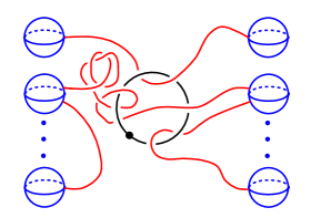
Figure 4.15. A 2-handlebody picture of the complement of the slice disk for $K$.

Proof.

The slicing disk can be seen in the picture as the disk filling the unknot that we have in the 1-sub-handlebody. This is since canceling the 1-2 handle pairs not only recovers $K$, but also recovers the ribbon disk $\widetilde{D}_{K}$. The definition of the dotted circle notation is that we remove a small neighborhood of the dotted unknot along with a small neighborhood of the disk after pushing it into $D^{4}$. And so this is exactly the complement of the slicing disk, $D^{4}-\widetilde{D}_{K}$. ∎

One nice fact is that, since disk slides, isotopies and handle cancellations can be done locally, and since ribbon knots always bound an immersed ribbon disk, this construction actually works in any 3-manifold. We did not rely on any special properties of $S^{3}$ during the process. One can create examples by combining a 2-handlebody picture for a ribbon knot $K\subset S^{3}$ as in the above construction with a Kirby picture of a 4-manifold $W$ whose boundary is the intended 3-manifold $M^{3}=\partial W$. When combining the two pictures, $K$ may be allowed to run across non-canceling 1-handles to form non-trivial examples as shown below. In Figure 4.16 we have a Kirby picture of a 4-manifold whose boundary is $S^{1}\times S^{2}$. We can see the ribbon disk for $K$ in the image on the left. The image on the right shows the result using the technique developed above.

\begin{overpic}[unit=1mm,scale={1}]{figure16b} \put(101.0,21.0){\hbox{\pagecolor{white}\parbox{2.84544pt}{$K$}}} \put(20.0,30.0){\hbox{\pagecolor{white}\parbox{2.84544pt}{$K$}}} \end{overpic}

Figure 4.16. An example ribbon knot in $S^{1}\times S^{2}$ and its decomposition.

References

- [EH1] J. B. Etnyre and K. Honda, Cabling and Transverse Simplicity, Annals of Math 162(2005), 1305-1333.
- [EH2] J. B. Etnyre and K. Honda, Knots and Contact Geometry, J. Symplectic Geom. 1 (2001), 63–120; math/0006112 .
- [ELT] J. B. Etnyre, D. J. LaFountain, B. Tosun, Legendrian and transverse cables of positive torus knots, Geometry & Topology 16 (2012) 1639–1689.
- [GS] R.E. Gompf and A.I. Stipsicz, 4-Manifolds and Kirby Calculus, American Mathematical Society. 1999.
- [H] K. Honda, On the Classification of Tight Contact Structures I, Geom. Topol. 4 (2000) 309-368.
- [Y] K.Yasui, Maximal Thurston-Bennequin Number and Reducible Legendrian Surgery, Compositio Mathematica, Volume 152, Issue 9, September 2016 , pp. 1899-1914.
- [K] Y. Kanda, The classification of tight contact structures on the 3-torus, Comm. Anal. Geom., 5 (1997), 413-438.
- [G] E. Giroux , Convexité en topologie de contact , Comm. Math. Helv. 66 (1991) 637–677.
- [EV] J. B. Etnyre and V. Vértesi, Legendrian Satellites, International Mathematics Research Notices, rnx106.
- [LS] T. Lidman and S. Sivek, Contact structures and reducible surgeries, Compositio Mathematica, Volume 152, Issue 1, January 2016, pp. 152-186.
- [CET] J. Conway, J. B. Etnyre, B. Tosun, Symplectic fillings, contact surgeries, and Lagrangian disks, arXiv:1712.07287 [math.GT].
- [Hed] M. Hedden, NOTIONS OF POSITIVITY AND THE OZSVÁTH-SZABÓ CONCORDANCE INVARIANT, Journal of Knot Theory Ramifications, 19, 617 (2010).
- [Eliash] Y Eliashberg , Classification of overtwisted contact structures on 3–manifolds , Invent. Math. 98 (1989) 623–637
- [Min] H. Min, Knots and uniform thickness property (work in progress).