Parallel loop cluster quantum Monte Carlo simulation of quantum magnets based on global union-find graph algorithm

Abstract

A large-scale parallel loop cluster quantum Monte Carlo simulation is presented. On 24,576 nodes of the K computer, one loop cluster Monte Carlo update of the world-line configuration of the $S=1/2$ antiferromagnetic Heisenberg chain with $2.6\times 10^{6}$ spins at inverse temperature $3.1\times 10^{5}$ is executed in about 8.62 seconds, in which global union-find cluster identification on a graph of about 1.1 trillion vertices and edges is performed. By combining the nonlocal global updates and the large-scale parallelization, we have virtually achieved about $10^{13}$-fold speed-up from the conventional local update Monte Carlo simulation performed on a single core. We have estimated successfully the antiferromagnetic correlation length and the magnitude of the first excitation gap of the $S=4$ antiferromagnetic Heisenberg chain for the first time as $\xi=1.040(7)\times 10^{4}$ and $\Delta=7.99(5)\times 10^{-4}$, respectively.

1 Introduction

The study of strongly-correlated quantum systems is the foremost area of research in contemporary statistical and condensed-matter physics [1], where the computational approaches are of increasing importance during recent years. From the viewpoint of the computational physics for the quantum lattice models, remaining challenges are: supersolid in frustrated spin/bosonic lattice models, where diagonal and offdiagonal long-range orders coexist [2]; cold atoms on optical lattice, in which one can compare experiments with computations directly [3]; deconfined criticality, a direct continuous quantum phase transition between long-range ordered phase with incompatible symmetries [4, 5, 6]; long-range and strongly anisotropic interactions, in which one observes effective reduction of spatial dimensions, exotic boundary effects, etc [7, 8, 9]. In order to tackle such fundamental and essential problems in strongly-correlated quantum systems, numerical simulations on large lattices are generally required, as the correlation length sometimes reaches millions of lattice constants and in many cases it indeed diverges due to strong fluctuations. Demands on unbiased and efficient simulation algorithms thus become stronger and stronger in recent years.

The quantum Monte Carlo method is one of the most promising tools as in principle it can simulate rather large lattices in any dimensions in statistically exact ways [10, 11, 12]. However, it is widely known that the conventional quantum Monte Carlo method based on local updates of world lines suffers from several drawbacks; ergodicity problem, fine-mesh slowing down, etc. Especially, in the vicinity of the criticality the autocorrelation time in the Markov chain diverges as $\xi^{z}$, where $\xi$ is the correlation length and $z\simeq 2$ is the dynamical exponent. This is called the critical slowing down. The loop algorithm invented in 1993 [13, 14] and its extensions solve (or at least reduce) most of the drawbacks in the conventional method [15, 16, 17].

The loop algorithm, which is a kind of cluster algorithm, realizes updates of world-line configuration by flipping nonlocal objects, called loops. It has been shown that it is fully ergodic and drastically reduces the autocorrelation time, often by orders of magnitude, especially at low temperatures. Furthermore, by using the continuous-time version of the algorithm, one can completely eliminate the discretization error originating from the Suzuki-Trotter decomposition; simulations can be performed directly in the so-called Trotter limit.

In high-performance computing, the importance of the non-floating-point operations (e.g., graph algorithms) has been widely realized these days, especially in the field of data-intensive applications [18]. Here, we present the world’s first peta-scale cluster algorithm quantum Monte Carlo simulation on the K computer based on global union-find algorithm on a graph of about 1.1 trillion vertices and edges, solving the fundamental problems in statistical and condensed-matter physics.

The organization of the present paper is as follows. After introducing the loop cluster algorithm, which is based on the nonlocal updates of world-line configuration by using the union-find graph algorithm, in Sec. 2, we discuss in detail how effectively the parallel graph algorithm is implemented using the OpenMP-MPI hybrid parallelization in Sec. 3. By using the highly parallelized loop cluster quantum Monte Carlo algorithm, we demonstrate in Sec. 4 that one Monte Carlo update of the world-line configuration of the $S=1/2$ antiferromagnetic Heisenberg chain with $2.6\times 10^{6}$ spins at inverse temperature $3.1\times 10^{5}$ is executed in about 8.62 seconds on 24,576 nodes of the K computer. By combining the nonlocal cluster updates and the large-scale parallelization on the K computer, we have virtually achieved about $10^{13}$-fold speed-up. In Sec. 5, we represent the result of the quantum Monte Carlo simulation of the $S=4$ antiferromagnetic Heisenberg chain. We have estimated successfully the antiferromagnetic correlation length and the magnitude of the first excitation gap for the first time as $1.040(7)\times 10^{4}$ and $7.99(5)\times 10^{-4}$, respectively. Finally, conclusions and some remarks are presented in Sec. 6.

2 The Loop Algorithm

We consider the antiferromagnetic Heisenberg model on a chain lattice of $L$ sites. The Hamiltonian is given by

$${\cal H}=J\sum_{j=1}^{L}{\bf S}_{j}\cdot{\bf S}_{j+1},$$ (1)

where the coupling constant $J>0$, and ${\bf S}_{j}=(S_{j}^{x},S_{j}^{y},S_{j}^{z})$ is the quantum spin operator at site $j$ with spin length $S$ satisfying the standard commutation relations, e.g., $[S_{j}^{x},S_{j}^{y}]=i\hbar S_{j}^{z}$. Hereafter, we set $J=1$ and assume periodic boundary conditions, ${\bf S}_{j+L}={\bf S}_{j}$. We consider the case with $S=1/2$ for a while. An extension to the higher-spin cases will be discussed in Sec. 5.

The expectation value of an observable $A$ is given by

$$\langle A\rangle={\rm Tr}\,A\exp(-\beta{\cal H})/Z,$$ (2)

where $Z$ is the partition function

$$Z={\rm Tr}\,\exp(-\beta{\cal H}),$$ (3)

$\beta=1/k_{\rm B}T$ the inverse temperature, $T$ the temperature, and $k_{\rm B}$ the Boltzmann constant. The density matrix $\exp(-\beta{\cal H})$ is regarded as an imaginary time evolution operator. Since the Hamiltonian ${\cal H}$ as well as the observable $A$ are $2^{L}\times 2^{L}$ matrices, the numerical diagonalization is feasible only for $L\lesssim 40$.

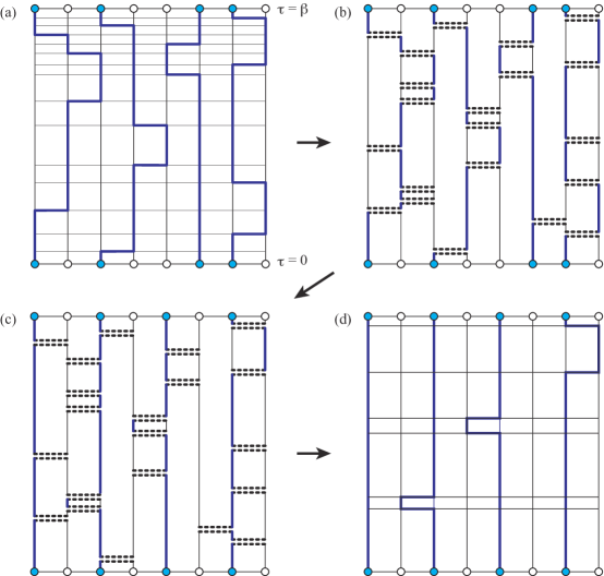
Figure 1: Example of one Monte Carlo step of the loop update for the antiferromagnetic Heisenberg chain with $L=8$. The horizontal and vertical axes correspond to the spatial and imaginary time directions, respectively. In (a) and (d), bold blue lines denote the world lines of up spins.

In the following, we work in a basis set $\{|\phi\rangle\}$ in which $S_{j}^{z}$ ($j=1\cdots L$) are diagonalized, i.e., $|\phi\rangle=|s_{1},\cdots s_{L}\rangle$ with $s_{j}=\uparrow,\downarrow$. We first split the density matrix into $M$ time slices:

$$Z={\rm Tr}\,[\exp(-\Delta_{\tau}{\cal H})]^{M}={\rm Tr}\,{\cal T}^{M}+{\cal O}(\beta^{2}/M),$$ (4)

where $\Delta_{\tau}=\beta/M$ and we have introduced the quantum transfer matrix ${\cal T}=1-\Delta_{\tau}{\cal H}$. After inserting ($M-1$) sums over a complete set of states, $\sum|\phi\rangle\langle\phi|=1$, between every ${\cal T}$, we obtain a path integral representation of the partition function:

$$Z \approx\!\!\sum_{\phi_{M},\cdots,\phi_{1}}\!\!\langle\phi_{1}|{\cal T}|\phi_{M}\rangle\langle\phi_{M}|{\cal T}|\phi_{M-1}\rangle\cdots\langle\phi_{2}|{\cal T}|\phi_{1}\rangle.$$ (5)

In the quantum Monte Carlo simulation, we sample the terms in the r.h.s. of Eq. (5) according to their magnitude. The matrix element $\langle\phi|{\cal T}|\phi^{\prime}\rangle$ is nonzero if and only if $|\phi\rangle=|\phi^{\prime}\rangle$, or they are identical except two neighboring spins that are swapped with one another, e.g., $|\phi\rangle=|\cdots\!\uparrow\downarrow\!\cdots\rangle$ and $|\phi^{\prime}\rangle=|\cdots\!\downarrow\uparrow\!\cdots\rangle$. These constraints for configurations can be depicted in terms of world lines [Fig. 1(a)]. Note that the diagonal elements in ${\cal T}$ are of ${\cal O}(1)$, while the nonzero offdiagonal elements are of ${\cal O}(\Delta_{\tau})$. Therefore, the number of jumps of world lines in the path integral representation remains finite even in the Trotter limit $M\rightarrow\infty$, and it is enough to store the spin configuration at $\tau=0$ and the space-time positions of jumps.

In the loop algorithm [13], given a world-line configuration, we first divide it into a set of closed loops as shown in Fig. 1(b). To be concrete, we assign local graphs according to the following rules: i) For an offdiagonal configuration, at which the world line jumps, a horizontal graph () is assigned with probability 1. ii) For a diagonal configuration with antiparallel spins ($\uparrow\downarrow$ or $\downarrow\uparrow$), a horizontal graph is assigned with probability $\Delta_{\tau}/2$, otherwise a vertical graph () is assigned. iii) For a diagonal configuration with parallel spins ($\uparrow\uparrow$ or $\downarrow\downarrow$), a vertical graph is assigned with probability 1. This procedure is called labeling or breakup.

Next, we flip each loop with probability 1/2. By this cluster flipping procedure, spins on each loop are flipped simultaneously from up to down or vice versa [Fig. 1(c)], and as a result a new world-line configuration is obtained [Fig. 1(d)]. It is straightforward to prove that the labeling procedure together with the cluster flipping procedure fulfills the balance condition as well as the ergodicity, so the Monte Carlo average of any physical quantities is guaranteed to converge to the correct value. Furthermore, the extent of loops corresponds directly to the antiferromagnetic spin correlation length in space-time. As a result, the correlations between successive world-line configurations are removed almost completely [15, 16, 17], and the autocorrelation time stays about few tens even for the largest systems we simulated below.

One should note that the labeling probability of a horizontal graph to the diagonal configuration is of ${\cal O}(\Delta_{\tau})$ and thus the total number of horizontal graphs also stays finite in the Trotter limit. In the practical implementation of the loop algorithm, therefore, we can work directly in the imaginary time continuum [19], which completely eliminates systematic errors due to the imaginary time discretization. To wrap up, one Monte Carlo step in the continuous imaginary time loop algorithm is as follows:

1. $\tau\leftarrow 0$ and $s\leftarrow(s_{1},s_{2},\cdots,s_{L}$) at $\tau=0$.

2. Draw a random number $r$ uniformly distributed in $(0,1]$, and $\tau^{\prime}\leftarrow\tau-(2/L)\log r$.

3. If there are offdiagonal operators between $\tau$ and $\tau^{\prime}$, assign a horizontal graph to them and update $s$ by flipping spins accordingly.

4. If $\tau^{\prime}>\beta$, go to step 7.

5. Draw a random integral number $l$ uniformly distributed in $(0,L]$, and insert a horizontal graph between sites $l$ and $l+1$ at imaginary time $\tau^{\prime}$, if $s_{l}\neq s_{l+1}$.

6. $\tau\leftarrow\tau^{\prime}$ and goto step 2.

7. Identify clusters, flip them independently with probability 1/2, and update spin configurations at $\tau=0$ and series of offdiagonal operators accordingly.

8. Perform measurement of physical quantities.

By inserting horizontal graphs in step 3 and 5, the space-time is decomposed into many small fragments of vertical lines [Fig. 1(b)]. Although each loop is a sequence of such fragments, it is more convenient to represent each loop by a rooted tree of segments instead of a sequential list. During step 2–6, trees are merged to build up loops by using the union-find algorithm [20]. It is proved that using two techniques, union-by-weight and path compression, any sequence of $m$ union and find operations on $n$ objects takes ${\cal O}(n\alpha(m,n))$ where $\alpha(m,n)$ is the inverse Ackerman function that grows extremely slow with increasing $m$ and $n$. In any practical applications, $\alpha(m,n)$ is less than 5 and one may regard it as a constant.

3 Parallelization of Loop Algorithm

The number of world-line jumps as well as the number of horizontal graphs are both proportional to $L\beta$, so is the total amount of the memory required to store the world-line configuration and the loop configuration. The number of operations required for one Monte Carlo sweep is also proportional to $L\beta$ as discussed in the last section. Since the autocorrelation time of the present loop algorithm is so short [$\sim{\cal O}(10)$] that the best parallelization strategy is running independent Markov chains with using different random number sequences on every node, as long as the memory requirement is not very strong. If $L\beta\gtrsim 10^{7}$, however, the world-line configuration no longer fits in the memory of one node, and parallelization of each Markov chain becomes unavoidable.

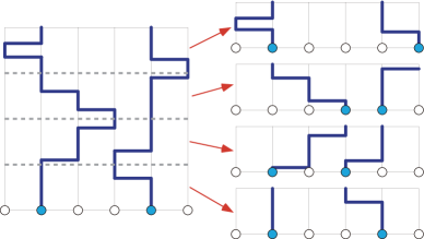
Figure 2: An example of MPI domain decomposition of world-line configuration for $L=6$ and 4 nodes. The horizontal and vertical axes are the spatial and imaginary time directions, respectively. The space-time is divided into slices of same thickness. Each node stores the spin directions at $\tau=\beta p/N_{\rm p}$ (circles) together with space-time positions of world-line jumps (horizontal blue lines) in its own time window.

3.1 Basic strategy

In general, parallelization of the loop algorithm is far from trivial, since a number of global objects, loops, are built up and flipped in every Monte Carlo step. The basic strategy for the nontrivial parallelization has been given in Refs. [21] and [22]. In order to parallelize the loop algorithm, first we have to determine how the information of world-line configuration is distributed to several nodes. In the continuous time loop algorithm for one-dimensional quantum spin systems, it is most natural to divide the (1+1)-dimensional space-time into $N_{\rm p}$ slices of thickness $\beta/N_{\rm p}$ in the imaginary time direction, where $N_{\rm p}$ is the number of nodes. Each node stores only the spin directions at imaginary time $\beta p/N_{\rm p}$, where $p$ is the processor index ($p=0,1,\cdots,N_{\rm p}-1$) together with space-time positions of world-line jumps in its own imaginary time window (Fig. 2). The same imaginary-time decomposition scheme can be used for higher-dimensional systems as well. One of the main advantages of this domain decomposition scheme is that the thickness of each slice can be chosen as the same regardless of the number of nodes or the network topology, as the system is continuous in the imaginary time direction. Another advantage of the present decomposition is that the algorithm does not depend on the dimensionality of the system.

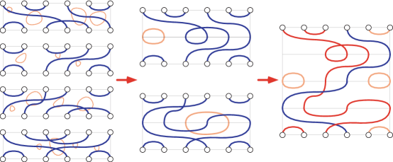
Figure 3: An example of the binary-tree global union-find procedure for $L=6$ and 4 nodes. Orange lines denote locally-closed loops, which can be ignored in the succeeding stages. In this case, one finally finds two global loops (red and blue loops in the rightmost figure) wrap around the whole system in the imaginary time direction.

By adopting the above domain decomposition scheme for the world-line configuration, the labeling procedure can be trivially parallelized and executed independently, since it requires local information only, i.e., the relative direction of two neighboring spins at the same imaginary time. No internode communication is required at this stage. On the other hand, identifying loops is nontrivial, since loops are global objects. We perform the global union-find procedure in the following two steps: (i) each node identifies loops in its own imaginary time window. In this step, a number of loops are closed in the time window. However, there remain $L$ unclosed loops, since they cross the imaginary-time boundaries between the nodes. This step requires no internode communication as the same as the labeling stage. Then, (ii) these unclosed loops are merged gradually by using a binary-tree algorithm as shown schematically in Fig. 3. Finally, the information on global loops is distributed back to all the nodes to determine the next world-line configuration. The number of operations required to the labeling process and the step (i) of the union-find process is proportional to $L\beta$ and these operations are ideally parallelized. On the other hand, the step (ii) of the union-find process can not be executed independently. The number of operations on the master node is proportional to $L\log_{2}N_{\rm p}$. Thus, the theoretical efficiency, $P(N_{\rm p})$, of the present parallelized loop algorithm is evaluated as

$$P(N_{\rm p})=\frac{\beta L}{N_{\rm p}}\Big{/}\Big{[}\frac{\beta L}{N_{\rm p}}+cL\log_{2}N_{\rm p}\Big{]}\simeq 1-c\frac{N_{\rm p}}{\beta}\log_{2}N_{\rm p}$$ (6)

for $\beta\gg N_{\rm p}$, where $c$ is a system-dependent constant.

Based on the above strategy, the parallel loop algorithm was first implemented using flat MPI, and it was confirmed that the code scales fairy well up to about $10^{3}$ nodes [21, 22]. In the environment with more than $10^{4}$ nodes ($10^{5}$ cores), however, it turns out that the overhead due to parallelization becomes non-negligible, and the simulation code does not scale any more. To overcome the difficulty, we have developed and implemented the following parallelization techniques.

3.2 Asynchronous wait-free union-find algorithm

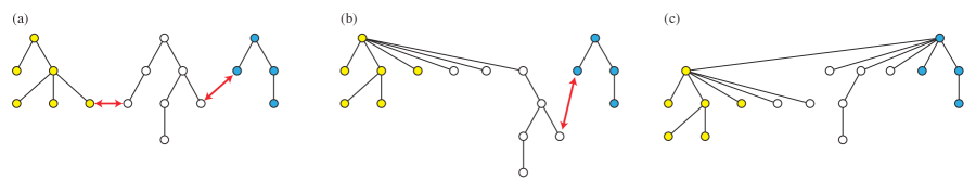
Figure 4: Example of a union-find procedure in which simultaneous update of trees can break the tree structures. The parent pointer of root vertex in the white tree can be rewritten simultaneously by two different threads.

The first improvement is the introduction of hybrid parallelization using OpenMP together with MPI. First of all, by introducing the MPI-OpenMP hybrid parallelization, the amount of memory used by the MPI library is reduced greatly compared with the case of using flat MPI parallelization. Second, introducing the parallelization with respect to another axis, the efficiency of parallelization can also be improved. In addition to the MPI process parallelization based on the domain decomposition in the imaginary time direction, we introduce OpenMP thread parallelization with respect to the real-space direction; the one-dimensional chain lattice is decomposed into domains with equal number of bonds (edges). Each thread maintains the list of operators on the bonds in its own domain, while the tree structure representing loops is shared globally by all threads in an MPI process. Since the union-find operations performed in each thread may alter the whole structure of trees, exclusive access control with high granularity must be introduced.

A union-find procedure of connecting two vertices A and B consists of the following steps:

1. Find the root vertex of A by tracking parent of vertices.

2. Find the root vertex of B by tracking parent of vertices.

3. Return if A and B belong to the same tree.

4. Compare the weight (number of vertices in each tree) of the root vertices, and choose a new root vertex.

5. Update the weight of the new root vertex.

6. Update the parent pointer of the other (new leaf) vertex.

7. Compress the path from vertices A and B to the new root vertex by rewriting the parent pointers of the vertices on the paths.

First, it should be noticed that in the union-find algorithm, once a vertex becomes a leaf vertex of a tree, then it never becomes back to a root vertex. Therefore, loops will never be created even if multiple threads try to alter the same tree simultaneously without access control. This guarantees that step 1–4 and 7 are already thread-safe, and we don’t need to modify these parts of the algorithm. On the other hand, we need to introduce some locking mechanism for step 5 and 6 to avoid breaking the tree structure by simultaneous updates of the parent pointer of the same root vertex by multiple threads (Fig. 4). The lock should be done vertex-wise so that the operation on different trees can be performed concurrently. At the same time, it should not require any extra memory, since the number of vertices are of ${\cal O}(L\beta)$. To this end, we have implemented the locking mechanism of each vertex by the inline assembler using the compare-and-swap atomic instruction (cmpxchgl in Intel64 architecture and cas in SPARC architecture). Thus, in the present thread-safe version of union-find algorithm, we modify step 5 and 6 as

1. Try to lock the two root vertices. If one or both lock trials fail, repeat from step 1.

2. Update the weight of the new root vertex.

3. Update the parent pointer of the other (new leaf) vertex.

4. Release the lock of the vertices.

This algorithm is thread-safe and wait-free. In practice, we implement this algorithm with no extra memory space by reusing the parent pointer (and weight) of each vertex as a lock object. Furthermore, the release of locks (in step 6’) will be done automatically by setting a new weight or the parent pointer in step 5 and 6. By this way, we can minimize the time window in which one or more vertices are in the locked state.

3.3 Butterfly-type global union-find algorithm

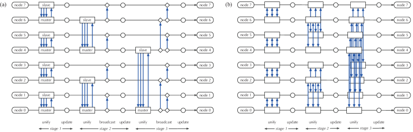
Figure 5: Patterns of communication in global union-find procedure using (a) binary-tree type and (b) butterfly type algorithms. In the former algorithm, the results of union-find at each stage have to be broadcasted to all the descendent nodes, which dominates the overall performance as the number of stages increases. On the other hand, in the latter algorithm combined with the majority-vote trick, the cost for each stage stays constant on hyper-torus networks.

The binary-tree global union-find algorithm described in Sec. 3.1 works fairy well up to $N_{\rm p}\simeq 10^{3}$ [21, 22, 23]. However, as the number of nodes is increased further, the overhead due to parallelization becomes non-negligible. The most dominant overhead is the cost for broadcasting the results of union-find procedure at each stage [Fig. 5(a)]. At each intermediate stage, $2L$ loop fragments are unified and as a result $L$ open loop fragments and a number of closed loops are obtained (Fig. 3). For the closed loops, we have to determine whether each of them will be flipped or not to generate the next world-line configuration, and broadcast the decision immediately to all the descendent nodes, since there is no memory space to store all the decisions until the whole union-find procedure is completed. Also, for the open loop fragments, we have to maintain the correspondence table between the original loop fragments to the new ones, and broadcast it to all the descendent nodes. For example, for $N_{\rm p}=24,576$, the total number of stages becomes 14 or 15, and at each stage we have to perform broadcast of the same order of depth.

In order to avoid the overhead of broadcast, we develop a butterfly-type global union-find algorithm. In this algorithm, the pattern of communication is modified as shown in Fig. 5(b), where instead of sending the loop fragment information from a slave to a master at each stage, two (or more) nodes exchange the loop fragment information with each other, then each of them performs the same union-find operations. By this way, broadcasting of the correspondence table is completely eliminated.

Note that in this butterfly-type algorithm, the union-find of loop fragments will be done out of order on each node. Accordingly, the tree structure built up on each node will also look completely different with each other, though final grouping of vertices (represented by trees) does not depend on the order of union-find operations and should be identical after the final stage has been completed. This fact makes it difficult for us to make globally consistent decisions on the loop flip, since the random number used for decisions generally depends on the execution order.

This difficulty is solved by introducing another technique, majority-vote trick. Instead of postponing the decision until loop fragments form a closed loop, we vote positive or negative on all loop fragments on each node in advance. The vote for each loop fragment is exchanged together with the other loop fragment information between nodes, and the number of positive and negative votes is counted in parallel with the union-find operation to make a final decision on the loop flip. Since the result of vote counting does not depend on its order, the decision for each loop will be globally consistent irrespective of the order of union-find operations. In practice, instead of counting positive and negative votes, we use XOR (exclusive-or) operations to tally the votes made for each loop in order to avoid ending in a draw accidentally.

3.4 Optimized process mapping on finite-dimensional torus

The butterfly-type global union-find algorithm works efficiently on a network with hypercube topology of dimension $\log_{2}N_{\rm p}$. On a lower-dimensional torus network, however, butterfly-type communication between distant nodes causes a network congestion in general, and the network transfer performance is often spoiled substantially. Moreover, if the linear extent of the torus network is not a power of 2, communications along different axes of the torus also interfere with each other. For example, the Tofu interconnect [24, 25] of the K computer logically provides a three-dimensional torus to users, and if a user wants to run a job by using the whole K computer, $48\times 54\times 32$ is the only possible shape of the three-dimensional torus, which is factored into $(2^{4}\times 3)\times(2\times 3^{3})\times 2^{5}$. In order to realize communication that is free from interference between different axes, one has to combine a pair-wise communication with three-point communication.

We have extended the global union-find algorithm, so that it works on generic virtual toruses of any dimensions, i.e., $\ell_{1}\times\ell_{2}\times\cdots\times\ell_{d}$ with any set of positive integers $(\ell_{1},\ell_{2},\cdots,\ell_{d})$. In $k$-th dimension of the virtual torus, which forms a set of periodic chains of length $\ell_{k}$, the union-find operations are repeated $\lfloor\ell_{k}/2\rfloor$ times (steps) by using only the two-sided nearest neighbor communication on that chain. In the above example, one can define the virtual torus as $(\ell_{1},\ell_{2},\ell_{3})=(48,54,32)$, in which we have no congestion but the total number of steps is relatively large ($24+27+16=67$). Another possibility is $(\ell_{1},\ell_{2},\cdots,\ell_{14})=((2,2,2,2,3),(2,3,3,3),(2,2,2,2,2))$, by which the total number of steps is minimized (14). There are many other possibilities between the extrema. There is a trade-off between the number of steps and severity of network congestion, and the optimal choice will depend on the system. Note that in the second example of the virtual torus, we introduce nested parentheses to emphasize that the product of lengths in each group is consistent with that of the original torus, and thus the inference between different axes of the original torus is avoided.

4 Performance Analysis

Based on the techniques presented in the last section, we have implemented the hybrid parallel version of the continuous time loop algorithm (ALPS/looper version 4 [26]) from the scratch by using the C++ programming language. The simulation code has been tested on 24,576 nodes (196,608 cores) of the K computer.

4.1 OpenMP thread parallelization

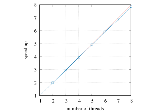
Figure 6: Strong scaling test of the asynchronous wait-free union-find algorithm in the Swendsen-Wang cluster algorithm for two-dimensional square lattice Ising model with $L=8,192$ and $K=K_{\rm c}=0.440686\cdots$. The red line indicates an ideal speed-up.

First, we test the efficiency of the asynchronous wait-free union-find algorithm, introduced in Sec. 3.2. As a benchmark test, we adopt the Swendsen-Wang cluster algorithm [27] for the two-dimensional square lattice Ising model. This algorithm is much simpler than the loop cluster algorithm, and thus more suitable for evaluating the performance the union-find algorithm directly. In the Ising model, we have classical spins $\sigma=\pm 1$ aligned to form an $L\times L$ two-dimensional array. In the Swendsen-Wang algorithm, the nearest neighbor sites are connected with probability $p=1-e^{-2K}$ if the spins on these sites have the same value. Then, the spins on each cluster are simultaneously flipped with probability 1/2. We choose the parameter $K$ as $K_{\rm c}=\ln(1+\sqrt{2})/2=0.440686\cdots$, the critical point of this model, where the average cluster size, which corresponds to the magnetic susceptibility diverges as $L^{7/4}$ with increasing the system size $L$ [28].

A benchmark test has been executed on a single node of the K computer. In Fig. 6, we show the result of the strong scaling test for $L=8,192$. We measure the execution time of the union-find operations during 128 Monte Carlo steps after discarding first 128 steps as burn-in time. The number of threads is 1, 2, 3, 4, 6, and 8. It takes about 0.097 second per Monte Carlo step in the single thread case. As one can see clearly in Fig. 6, almost perfect strong scaling has been achieved up to 8 threads. The parallelization efficiency is about 98.2% if one compares the 8-thread performance with the single thread case.

4.2 Network performance

Table 1: Network transfer performance on 12,288 nodes of the K computer. The shape of three-dimensional torus is $32\times 12\times 32$ and the shape of virtual lattice (transfer pattern) is chosen as $((2,2,2,2,2),(2,2,3),(2,2,2,2,2))$.

stage	$\ell_{k}$	transfer rate [GB/sec]	multiplicity	efficiency [%]
1	2	4.44	1	88.8
2	2	2.26	2	90.4
3	2	1.13	4	90.4
4	2	0.56	8	89.6
5	2	0.56	8	89.6
6	2	4.44	1	88.8
7	2	2.26	2	90.4
8	3	1.50	4	120.0
9	2	4.32	1	86.4
10	2	2.26	2	90.4
11	2	1.13	4	90.4
12	2	0.56	8	89.6
13	2	0.56	8	90.6

We demonstrate the effectiveness of the process mapping strategy introduced in Sec. 3.4 by using 12,288 nodes of the K computer. The shape of three-dimensional torus is $32\times 12\times 32$. We choose a 13-dimensional virtual lattice whose shape is given by $((2,2,2,2,2),(2,2,3),(2,2,2,2,2))$, so that there occurs no interference between different axes. In the benchmark program, a continuous data of 10 MB is transferred in each stage in both directions between nodes. In Table. 1, we summarize the network transfer performance at each stage. At stage 1, 6, 9, the data transfer is performed between adjacent nodes on the three-dimensional torus. In these cases the transfer rate is 4.32–4.44 GB/s which is about 86.4–88.8% of the theoretical peak bandwidth 5 GB/s. At stage 2, 7, 10, each link between the nodes is shared by two communications. Taking into account that the multiplicity of the link is 2, the efficiency is evaluated as 90.4%. The multiplicity of each stage is given by the product of lengths ($\ell_{k}$) of earlier stages in the current axis. In the final stage of each axis, if $\ell_{k}=2$, the multiplicity becomes half, since the other side of the periodic chain can be utilized simultaneously. For example, we estimate the multiplicity of stage 4 (13) is $2\times 2\times 2=8$ ($2\times 2\times 2\times 2\,/\,2=8$). Remarkably, the efficiency is not degraded even for the case with 8-fold multiplicity (stage 4, 5, 12, 13). The efficiency is as high as the case of adjacent communication, and there is absolutely no signs of network congestion.

We should point out that at stage 8, which has $\ell_{k}=3$ and 4-fold multiplicity according to the above rule, shows performance much higher than the theoretical peak. This unforeseen performance may owe to the physical structure of the Tofu network, i.e., 6-dimensional mesh/torus of $32^{3}\times 2\times 3\times 2$ [24, 25]. Indeed, by assuming 90 % of the theoretical peak, we can estimate the effective multiplicity as

$$5\times 0.9/1.50\simeq 3,$$ (7)

which manifests the existence of extra links hidden from the three-dimensional logical view of the torus.

4.3 Weak scaling property

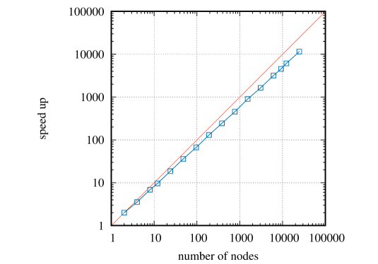
Figure 7: Weak scaling results for $N_{\rm p}=2$, 4, 8, 12, 24, 48, 96, 192, 384, 768, 1,536, 3,072, 6,144, 9,216, 12,288, and 24,576. The parallelization efficiency for $N_{\rm p}=24,576$ is about 46.9%. The red line denotes the ideal speed-up.

The efficiency of the present OpenMP-MPI hybrid parallelized continuous time loop algorithm is demonstrated by the weak scaling test up to 24,576 nodes (196,608 cores) of the K computer. In this weak scaling test, the system size is fixed to $L=2,621,440$ and the inverse temperature is increased in proportional to the number of nodes as $\beta=12.642N_{\rm p}$. The number of threads in each process is 8, and the number of nodes, which is the same as the number of processes, is tested starting from $N_{\rm p}=2$ up to 24,576. The overall speed-up as a function of $N_{\rm p}$ is shown in Fig. 7, where the speed-up at $N_{\rm p}=2$ is normalized to 2. With $N_{\rm p}=24,576$, we have achieved speed-up by a factor of $1.1\times 10^{4}$. The parallelization efficiency is thus about 46.9%.

The decline of the efficiency is mainly due to the overhead of global union-find operations. In Fig. 8, we show the $N_{\rm p}$-dependence of the cost of each section. One sees that the cost of global union-find operation as well as that of the communication grow in proportional to $\log_{2}N_{\rm p}$, while the cost of labeling and the local union-find operations stays constant irrespective of the number of nodes. This behavior is consistent with the theoretical estimation given in the last section [Eq. (6)].

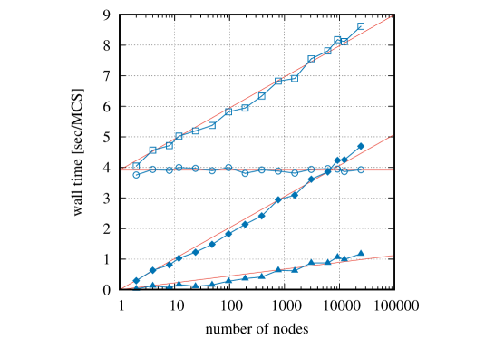
Figure 8: $N_{\rm p}$-dependence of the cost of each section: whole Monte Carlo step (squares), labeling and local union-find (circles), global union-find including communication (filled diamonds), communication (filled triangles). The cost for global union-find as well as that for communication is roughly proportional to $\log_{2}N_{\rm p}$.

Table 2: Cost distribution in one Monte Carlo step for 12,288 and 24,576 nodes on the K computer.

	12,288 nodes [sec]	24,576 nodes [sec]
1) random number generation in exponential distribution	0.53	0.54
2) insert/remove operators and local union-find operations	1.77	1.83
3) assignment of loop IDs	0.33	0.33
4) accumulation physical properties of loops	0.91	0.91
5) global union-find operations (except for communication)	3.26	3.52
6) pair-wise communication	0.91	1.09
7) three-point communication	0.08	0.09
8) update of spins and operators	0.32	0.32
5+6+7	4.25	4.69
total	8.12	8.62

The detailed comparison of the cost between the cases with $N_{\rm p}=12,288$ and 24,576 is given in Table 2. For $N_{\rm p}=12,288$, we choose the shape of three-dimensional torus as $16\times 24\times 32$ and that of virtual lattice as $((2,2,2,2),(2,2,2,3),(2,2,2,2,2))$. For $N_{\rm p}=24,576$ the length along the first axis of the torus is doubled and the shape of virtual lattice is chosen as $((2,2,2,2,2),(2,2,2,3),(2,2,2,2,2))$. We attribute the slight growth in section 2 to fluctuations between nodes due to some system noise. The growth of cost in section 6 (pair-wise communication), which is the summation of the communication cost of stages with $\ell_{k}=2$, should be explained based on the network performance analysis in the previous subsection. Taking into account that the length along the first axis of the torus is doubled from 16 to 32, the growth of the cost is estimated as

$$\frac{(1+2+4+8+8)+(1+2+4)+(1+2+4+8+8)}{(1+2+4+4)+(1+2+4)+(1+2+4+8+8)}\simeq 1.29,$$ (8)

which is consistent with the experiments, $1.09/0.91\simeq 1.20$. Similarly, the growth of cost in section 5 [global union-find (except for communication)] ($3.52/3.26\simeq 1.08$) can be explained by the increase of the number of stages ($14/13\simeq 1.08$).

4.4 Overall performance

With 24,576 nodes of the K computer, we simulate a chain with 2,621,440 spins at inverse temperature 310,690. The space-time volume is thus $L\beta\simeq 8.14\times 10^{11}$. The average number of operators (or horizontal graphs) is about $5.64\times 10^{11}$. One Monte Carlo step takes about 8.62 seconds. In each Monte Carlo steps, we generate a graph of $1.13\times 10^{12}$ vertices (world-line fragments) and $1.13\times 10^{12}$ edges, and identify clusters by performing union-find operations on such a huge graph, resulting $3.24\times 10^{11}$ clusters in average. Note that size of the largest cluster is of the same order as the space-time volume $\sim 10^{12}$ as the ground state of the present $S=1/2$ antiferromagnetic Heisenberg chain is critical and thus the correlation length is infinite in the thermodynamic limit.

Since the most time consuming part in the present algorithm is the union-find operations on the tree structure, the performance index concerning floating-point operations is not impressive. The overall performance using 24,576 nodes is 7.63 TFLOPS (tera floating-point operations per second) and 0.164 PIPS (peta instructions per second), which are 0.243% and 10.4% of the theoretical peak performance, 3.15 PFLOPS ($=10^{3}$ TFLOPS) and 1.57 PIPS, respectively.

Table 3: Ground-state energy density $E/L$, staggered susceptibility $\chi_{\rm s}$, spatial correlation length $\xi$, first excited gap $\Delta$ of $S=1$, 2, 3, 4 antiferromagnetic Heisenberg chains estimated by various numerical methods: MCPM (Monte Carlo Power Method), RSRG (Real Space Renormalization Group), QMC (Quantum Monte Carlo), DMRG (Density Matrix Renormalization Group), ND (Numerical Diagonalization).

$S$	$E/L$	$\chi_{\rm s}$	$\xi$	$\Delta$	method
1	-1.4015(5)			0.41	MCPM [29]
	-1.449724			0.368166	RSRG [30]
	-1.4021(5)			0.4097(5)	RSRG [31]
			6.25	0.425	QMC [32]
	-1.401484038971(4)		6.03(2)	0.41050(2)	DMRG [33]
	-1.401485(2)		6.2	0.41049(2)	ND [34]
	-1.401481(4)	18.4048(7)	6.0153(3)	0.41048(6)	QMC [23]
				0.41047777	ND (lower bound) [35]
				0.41048023	ND (upper bound) [35]
2			80	0.08	QMC [36]
			80	0.02	QMC [37]
	-4.7608		33	0.02	DMRG [38]
	-4.7545			0.05	QMC [39]
	-4.761248(1)		49(1)	0.085(5)	DMRG [40]
	-4.76125(5)			0.082(3)	DMRG [41]
	-4.761244(1)		54.3(2)	0.085(1)	DMRG [42]
		$1.16(1)\times 10^{3}$	50(1)	0.090(5)	QMC [43]
				0.0907(2)	DMRG [44]
				0.0876(13)	DMRG [45]
	-4.761249(6)	$1.1640(2)\times 10^{3}$	49.49(1)	0.08917(4)	QMC [23]
				0.0878	ND (lower bound) [35]
				0.0896	ND (upper bound) [35]
			49.6(1)	0.0891623(9)	DMRG [46]
				0.0884	ND (lower bound) [47]
				0.0896	ND (upper bound) [47]
3	-10.1239(1)	$1.580(3)\times 10^{5}$	637(1)	0.01002(3)	QMC [23]
				0.0082	ND (lower bound) [35]
				0.0102	ND (upper bound) [35]
4				$6.3\times 10^{-4}$	ND (lower bound) [35]
				$8.1\times 10^{-4}$	ND (upper bound) [35]
	-17.480(7)	$3.49(4)\times 10^{7}$	$1.040(7)\times 10^{4}$	$7.99(5)\times 10^{-4}$	QMC (present work)

5 Estimation of the Haldane Gap of $S=4$ Chain

The ground state of the $S=1/2$ antiferromagnetic Heisenberg chain [Eq. (1)] is known to be critical, where the antiferromagnetic correlation function decays algebraically as the distance increases, and above the ground state there are gapless excitations [48]. On the other hand, in the classical limit ($S\rightarrow\infty$), each spin behaves as a classical vector, and the ground state is the long-range ordered Néel state. It again has gapless spin-wave excitations.

In 1982, Haldane [49] made a striking conjecture that the antiferromagnetic Heisenberg chain with integer $S$ ($S=1,2,\cdots$) has a finite excitation gap $\Delta(S)$ above its unique ground state, and the antiferromagnetic spin correlation along the chain decays exponentially with a finite correlation length $\xi(S)$. For the $S=1$, 2, and 3, the finiteness of the first excitation gap as well as the correlation length has already been established numerically as listed in Table 3. Simulations of higher-spin systems, however, are much harder since the excitation gap (the correlation length) becomes exponentially small (large) as $S$ increases [49]. The main difficulty for measuring such a small gap is that the system behaves as if gapless (critical) so long as the temperature is not low enough compared to the gap. Similarly, the system size used in the simulation should be much larger than the correlation length to detect a finite correlation length. Thus we need to simulate extremely large systems at extremely low temperatures in order to access the low-energy properties of the higher-spin systems, and precise estimation of $\Delta(S)$ and $\xi(S)$ for $S=4$, 5, $\cdots$ is still being one of the most challenging problems in the computational statistical and condensed-matter physics.

Let us consider the antiferromagnetic Heisenberg chain (1) with $S=4$. In order to apply the continuous time loop algorithm to the this system, first we represent the $S=4$ system by an equivalent $S=1/2$ system; each $S=4$ spin is represented as a composition of 8 $S=1/2$ spins (subspins), and simultaneously each bond is transformed into 64 bonds of the same strength connecting subspins [50, 23]. The largest system we simulate is $L=73,728$ ($=2^{13}\times 3^{2}$), which is converted in advance into an equivalent $S=1/2$ system of $8\times 73,728$ sites and $64\times 73,728$ bonds. The inverse temperature is chosen as $\beta=L/(2S)=9216$.

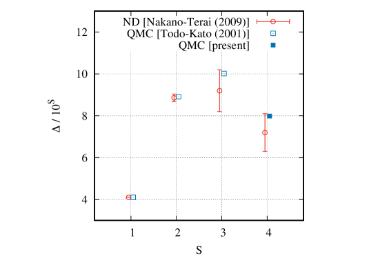
Figure 9: $S$-dependence of the first excitation gap of the spin-$S$ antiferromagnetic Heisenberg models calculated by the quantum Monte Carlo method (blue symbols) [23]. Note that $\Delta\times 10^{S}$ is plotted instead of $\Delta$ itself, since it decreases exponentially as $S$ increases. The error bar of each data point is smaller than the symbol size. A lower and upper bounds estimated by the numerical diagonalization (ND) are also indicated by red lines [35].

The simulation is performed by using 2,048 nodes. About 10 GB of memory is required per node ($\sim$ 20 TB in total) in order to store the world-line and loop configurations. The correlation length and the magnitude of the gap are calculated by means of the higher-order version of the moment estimators [23, 51]. The measurement is performed during 8,192 Monte Carlo steps after discarding first 1,024 steps as burn-in time. By the jackknife analysis, the mean values and their error bars (1$\sigma$) are finally evaluated as

$$\xi =1.040(7)\times 10^{4}$$ (9)

$$\Delta =7.99(5)\times 10^{-4}.$$ (10)

Since $\beta\Delta>6$ and $L/\xi>6$ are both satisfied, we can empirically regard the present estimates as those in the thermodynamic and the zero-temperature limits [23, 52]. The final estimate of $\Delta$ for $S=4$ is plotted in Fig. 9 together with those for $S=1$, 2, 3 obtained by the previous quantum Monte Carlo simulations [23]. It is clearly seen that $\Delta(S)$ decreases exponentially as $S$ increases. The present result for the gap can be compared with the lower and upper bounds for the gap obtained by means of the numerical diagonalization [35]. The present result is in between the lower and upper bounds, but it’s quite close to the upper bound. On the other hand, the result for the correlation length in the real-space direction is new to the best of our knowledge.

It should be emphasized that the present results are obtained without any extrapolation procedure; they are simply obtained by a single Monte Carlo run on the largest system at the lowest temperature. Thus, the highly parallelized continuous time loop algorithm is proved to be a sensitive numerical tool that can distinguish a system with extremely small excitation gap ($\sim 10^{-3}$) from a critical one, and will certainly be necessary in investigating the properties of novel quantum critical phenomena in future theoretical studies in the statistical and condensed-matter physics.

6 Conclusion

In the present paper, we discuss the parallel quantum Monte Carlo method that can simulate millions of spins at extremely low temperatures ($\sim 10^{-6}$). By using the nonlocal update scheme based on the union-find graph algorithm, one can simulate such a huge system without any convergence problem. We show that the global graph algorithm is performed very efficiently up to 24,576 nodes (196,608 cores) of the K computer by means of the OpenMP-MPI hybrid scheme combined with several new techniques; asynchronous wait-free union-find algorithm, butterfly-type global union-find algorithm, majority-vote trick, process mapping optimization, etc. In conclusion, we have achieved $8\,(\text{threads})\times 98.2\%\times 24,576\,(\text{nodes})\times 46.9\%\simeq 10^{5}$-fold speed-up by parallelization. Together with $\xi^{2}\simeq 10^{8}$-fold acceleration of the Monte Carlo dynamics by eliminating the critical slowing down by the nonlocal cluster updates, we have virtually achieved $10^{13}$-fold speed-up in total compared with the conventional local update quantum Monte Carlo updates performed on a single core. The present parallelization scheme can be extended to other models, such as the spin system with SU($N$) symmetry and the four-body interaction [5, 6], the transverse-field Ising model, etc.

References

- [1] A. Avella, F. Mancini (Eds.), Strongly Correlated Systems: Theoretical Methods, Springer-Verlag, Berlin, 2011.
- [2] K. Yamamoto, S. Todo, S. Miyashita, Successive phase transitions at finite temperatures toward the supersolid state in a three-dimensional extended Bose-Hubbard model, Phys. Rev. B 79 (2009) 094503. doi:10.1103/PhysRevB.79.094503.
- [3] J.-W. Huo, F.-C. Zhang, W. Chen, M. Troyer, U. Schollwöck, Trapped ultracold bosons in periodically modulated lattices, Phys. Rev. A 84 (2011) 043608. doi:10.1103/PhysRevA.84.043608.
- [4] T. Senthil, A. Vishwanath, L. Balents, S. Sachdev, M. P. A. Fisher, Deconfined quantum critical points, Science 303 (2004) 1490. doi:10.1126/science.1091806.
- [5] K. Harada, T. Suzuki, T. Okubo, H. Matsuo, J. Lou, H. Watanabe, S. Todo, N. Kawashima, Possibility of deconfined criticality in SU() Heisenberg models at small , Phys. Rev. B 88 (2013) 220408(R). doi:10.1103/PhysRevB.88.220408.
- [6] T. Suzuki, K. Harada, H. Matsuo, S. Todo, N. Kawashima, Thermal phase transition of generalized Heisenberg models for spins on square and honeycomb lattices, Phys. Rev. B 91 (2015) 094414. doi:10.1103/PhysRevB.91.094414.
- [7] C. Yasuda, S. Todo, K. Hukushima, F. Alet, M. Keller, M. Troyer, H. Takayama, Néel temperature of quasi-low-dimensional Heisenberg antiferromagnets, Phys. Rev. Lett. 94 (2005) 217201. doi:10.1103/PhysRevLett.94.217201.
- [8] S. Yasuda, H. Suwa, S. Todo, Stochastic approximation of dynamical exponent at quantum critical point, Phys. Rev. B 92 (2015) 104411. doi:10.1103/PhysRevB.92.104411.
- [9] T. Horita, H. Suwa, S. Todo, Upper and lower critical decay exponents of Ising ferromagnet with long-range interaction, Phys. Rev. E 95 (2017) 012143. doi:10.1103/PhysRevE.95.012143.
- [10] M. Suzuki (Ed.), Quantum Monte Carlo Methods in Condensed Matter Physics, World Scientific, Singapore, 1994.
- [11] D. P. Landau, K. Binder, A Guide to Monte Carlo Simulations in Statistical Physics, 4th Edition, Cambridge University Press, Cambridge, 2014.
- [12] J. Gubernatis, N. Kawashima, W. Philipp, Quantum Monte Carlo Methods: Algorithms for Lattice Models, Cambridge University Press, Cambridge, 2016.
- [13] H. G. Evertz, G. Lana, M. Marcu, Cluster algorithm for vertex models, Phys. Rev. Lett. 70 (1993) 875. doi:10.1103/PhysRevLett.70.875.
- [14] U.-J. Wiese, H.-P. Ying, A determination of the low energy parameters of the 2-d Heisenberg antiferromagnet, Z. Phys. B 93 (1994) 147. doi:10.1007/BF01316955.
- [15] H. G. Evertz, The loop algorithm, Adv. in Physics 52 (2003) 1. doi:10.1080/0001873021000049195.
- [16] N. Kawashima, K. Harada, Recent development of world-line Monte Carlo methods, J. Phys. Soc. Jpn. 73 (2004) 1379. doi:10.1143/JPSJ.73.1379.
- [17] S. Todo, Loop algorithm, in: A. Avella, F. Mancini (Eds.), Numerical Methods for Strongly Correlated Systems, Springer-Verlag, Berlin, 2012.
- [18] http://www.graph500.org/.
- [19] B. B. Beard, U. J. Wiese, Simulations of discrete quantum systems in continuous Euclidean time, Phys. Rev. Lett. 77 (1996) 5130.
- [20] T. H. Cormen, C. E. Leiserson, R. L. Rivest, C. Stein, Introduction to Algorithms, 2nd Edition, MIT Press, Cambridge, 2001.
- [21] S. Todo, Quantum cluster algorithm Monte Carlo method and its application to higher-spin Heisenberg antiferromagnets, Prog. Theor. Phys. Suppl. 145 (2002) 188. doi:10.1143/PTPS.145.188.
- [22] S. Todo, Parallel quantum Monte Carlo simulation of antiferromagnetic Heisenberg chain, in: D. P. Landau, S.-P. Lewis, H.-B. Schüttler (Eds.), Computer Simulation Studies in Condensed Matter Physics XV, Springer-Verlag, Berlin, 2003, p. 89.
- [23] S. Todo, K. Kato, Cluster algorithms for general- quantum spin systems, Phys. Rev. Lett. 87 (2001) 047203. doi:10.1103/PhysRevLett.87.047203.
- [24] Y. Ajima, S. Sumimono, S. Shimizu, Tofu: A 6D mesh/torus interconnect for exascale computers, IEEE Computer 42 (2009) 36. doi:10.1109/MC.2009.370.
- [25] T. Toyoshima, ICC: An interconnect controller for the Tofu interconnect architecture, HOT CHIPS 22 (2010).
- [26] https://github.com/wistaria/alps-looper.
- [27] R. H. Swendsen, J. S. Wang, Nonuniversal critical dynamics in Monte Carlo simulations, Phys. Rev. Lett. 58 (1987) 86. doi:10.1103/PhysRevLett.58.86.
- [28] N. Goldenfeld, Lectures on Phase Transitions and the Renormalization Group, Addison-Wesley, Reading, Massachusetts, 1992.
- [29] M. P. Nightingale, H. W. J. Blöte, Gap of the linear spin-1 Heisenberg antiferromagnet: A Monte Carlo calculation, Phys. Rev. B 33 (1986) 659. doi:10.1103/PhysRevB.33.659.
- [30] C. Y. Pan, X. Chen, Renormalization-group study of high-spin Heisenberg antiferromagnets, Phys. Rev. B 36 (1987) 8600. doi:10.1103/PhysRevB.36.8600.
- [31] Lin, H. Q., Pan, C. Y., Renormalization group study of the anisotropic and alternating Heisenberg antiferromagnets, J. Phys. Colloques 49 (1988) C8–1415. doi:10.1051/jphyscol:19888650.
- [32] K. Nomura, Spin correlation function of the antiferromagnetic Heisenberg chain by the large-cluster-decomposition Monte Carlo method, Phys. Rev. B 40 (1989) 2421. doi:10.1103/PhysRevB.40.2421.
- [33] S. R. White, D. A. Huse, Numerical renormalization-group study of low-lying eigenstates of the antiferromagnetic Heisenberg chain, Phys. Rev. B 48 (1993) 3844. doi:10.1103/PhysRevB.48.3844.
- [34] O. Golinelli, T. Jolicoeur, R. Lacaze, Finite-lattice extrapolations for a Haldane-gap antiferromagnet, Phys. Rev. B 50 (1994) 3037. doi:10.1103/PhysRevB.50.3037.
- [35] H. Nakano, A. Terai, Reexamination of finite-lattice extrapolation of Haldane gaps, J. Phys. Soc. Jpn. 78 (2009) 014003. doi:10.1143/JPSJ.78.014003.
- [36] J. Deisz, M. Jarrell, D. L. Cox, Dynamical properties of one-dimensional antiferromagnets: A Monte Carlo study, Phys. Rev. B 48 (1993) 10227. doi:10.1103/PhysRevB.48.10227.
- [37] N. Hatano, M. Suzuki, Correlation length of the antiferromagnetic Heisenberg chain, J. Phys. Soc. Jpn. 62 (1993) 1346. doi:10.1143/JPSJ.62.1346.
- [38] S. Qin, T.-K. Ng, Z.-B. Su, Edge states in open antiferromagnetic Heisenberg chains, Phys. Rev. B 52 (1995) 12844. doi:10.1103/PhysRevB.52.12844.
- [39] G. Sun, Numerical solution of the spin-2 Heisenberg antiferromagnetic chains using a projector method, Phys. Rev. B 51 (1995) 8370. doi:10.1103/PhysRevB.51.8370.
- [40] U. Schollwöck, T. Jolicoeur, Haldane gap and hidden order in the antiferromagnetic quantum spin chain, Europhys. Lett. 30 (1995) 493. doi:10.1209/0295-5075/30/8/009.
- [41] S. Qin, Y.-L. Liu, L. Yu, Finite-size scaling for low-energy excitations in integer Heisenberg spin chains, Phys. Rev. B 55 (1997) 2721. doi:10.1103/PhysRevB.55.2721.
- [42] S. Qin, X. Wang, L. Yu, Universality class of integer quantum spin chains: case study, Phys. Rev. B 56 (1997) R14251. doi:10.1103/PhysRevB.56.R14251.
- [43] Y. J. Kim, M. Greven, U.-J. Wiese, R. J. Birgeneau, Monte-Carlo study of correlations in quantum spin chains at non-zero temperature, Euro. Phys. J. B 4 (1998) 291. doi:10.1007/s100510050382.
- [44] U. Schollwöck, Marshall’s sign rule and density-matrix renormalization-group acceleration, Phys. Rev. B 58 (1998) 8194. doi:10.1103/PhysRevB.58.8194.
- [45] X. Wang, S. Qin, L. Yu, Haldane gap for the antiferromagnetic Heisenberg chain revisited, Phys. Rev. B 60 (1999) 14529. doi:10.1103/PhysRevB.60.14529.
- [46] H. Ueda, K. Kusakabe, Determination of boundary scattering, magnon-magnon scattering, and the Haldane gap in Heisenberg spin chains, Phys. Rev. B 84 (2011) 054446. doi:10.1103/PhysRevB.84.054446.
- [47] H. Nakano, T. Sakai, Precise estimation of the Haldane gap by numerical diagonalization, J. Phys. Soc. Jpn. 87 (2018) 105002. doi:10.7566/JPSJ.87.105002.
- [48] J. des Cloizaux, J. J. Pearson, Spin-wave spectrum of the antiferromagnetic linear chain, Phys. Rev. 128 (1962) 2131.
- [49] F. D. M. Haldane, Spontaneous dimerization in the Heisenberg antiferromagnetic chain with competing interactions, Phys. Rev. B 25 (1982) 4925. doi:10.1103/PhysRevB.25.4925.
- [50] K. Harada, M. Troyer, N. Kawashima, The two-dimensional quantum Heisenberg antiferromagnet at finite temperatures, J. Phys. Soc. Jpn. 67 (1998) 1130. doi:10.1143/JPSJ.67.1130.
- [51] H. Suwa, S. Todo, Generalized moment method for gap estimation and quantum Monte Carlo level spectroscopy, Phys. Rev. Lett. 115 (2015) 080601. doi:10.1103/PhysRevLett.115.080601.
- [52] S. Todo, M. Matsumoto, C. Yasuda, H. Takayama, Plaquette-singlet solid state and topological hidden order in a spin-1 antiferromagnetic Heisenberg ladder, Phys. Rev. B 64 (2001) 224412. doi:10.1103/PhysRevB.64.224412.
- [53] B. Bauer, L. D. Carr, H. G. Evertz, A. Feiguin, J. Freire, S. Fuchs, L. Gamper, J. Gukelberger, E. Gull, S. Guertler, A. Hehn, R. Igarashi, S. V. Isakov, D. Koop, P. N. Ma, P. Mates, H. Matsuo, O. Parcollet, G. Pawlowski, J. D. Picon, L. Pollet, E. Santos, V. W. Scarola, U. Schollwöck, C. Silva, B. Surer, S. Todo, S. Trebst, M. Troyer, M. L. Wall, P. Werner, S. Wessel, The ALPS project release 2.0: open source software for strongly correlated systems, J. Stat. Mech.: Theo. Exp. (2011) P05001doi:10.1088/1742-5468/2011/05/P05001.
- [54] http://alps.comp-phys.org/.