Theoretical and numerical studies on global stability of traveling waves with oscillations for time-delayed nonlocal dispersion equations

Abstract

This paper is concerned with the global stability of non-critical/critical traveling waves with oscillations for time-delayed nonlocal dispersion equations. We first theoretically prove that all traveling waves, especially the critical oscillatory traveling waves, are globally stable in a certain weighted space, where the convergence rates to the non-critical oscillatory traveling waves are time-exponential, and the convergence to the critical oscillatory traveling waves are time-algebraic. Both of the rates are optimal. The approach adopted is the weighted energy method with the fundamental solution theory for time-delayed equations. Secondly, we carry out numerical computations in different cases, which also confirm our theoretical results. Because of oscillations of the solutions and nonlocality of the equation, the numerical results obtained by the regular finite difference scheme are not stable, even worse to be blow-up. In order to overcome these obstacles, we propose a new finite difference scheme by adding artificial viscosities to both sides of the equation, and obtain the desired numerical results.

Keywords: Critical traveling waves, time-delay, global stability, nonlocal dispersion equation, oscillations.

AMS subject classifications. 35K57, 35B35, 35C07, 35K15, 35K58, 92D25

1 Introduction

In this paper, we consider the global stability of critical oscillatory traveling waves for a class of nonlocal dispersion equations with time-delay

$$\begin{cases}\displaystyle\frac{\partial v}{\partial t}-D(J*v-v)+d(v)=K*b(v(t-r,\cdot)),\quad&x\in\mathbb{R},~{}t>0,\\ v(s,x)=v_{0}(s,x),\quad&x\in\mathbb{R},~{}s\in[-r,0],\end{cases}$$ (1.1)

where the initial value satisfies

$$\lim_{x\to\pm\infty}v_{0}(s,x)=v_{\pm},~{}\text{uniformly in}~{}s\in[-r,0].$$

This model represents the spatial dynamics of a single-species population with age-structure and nonlocal diffusion such as the Australian blowflies population distribution [8, 9]. Here $v(t,x)$ denotes the total mature population of the species, the function $d(v)$ and $b(v)$ are the death and birth rates of the mature population respectively, $J(x)$ and $K(x)$ are non-negative, unit and symmetric kernels, $J(x)$ is the probability distribution of rates of dispersal over distance $x$. Then $J*v(x)$ is the rate at which individuals are arriving at position $x$ from all other locations, and $v(x)=\int_{\mathbb{R}}J(x,y)v(x)dy$ is the rate at which they are leaving location $x$ to travel to all other sites. Therefore, the expression $D(J*v-v)$ is the nonlocal dispersion due to long range dispersion mechanisms [5, 12], where the coefficient $D>0$ is the spatial diffusion rate.

The advantages of the nonlocal process governed by integral process over the classical dispersal process modelled by Laplacian lie in the fact that the nonlocal one accounts for interaction between individual in both short and long ranges, while the classical one accounts for only local interactions between the neighbor individuals. Moreover, the nonlocal operator for the initial value problem is not a smoothing operator. Discontinuities in the initial data are retained [5]. And the spatial decay rates of the traveling waves at infinity are different in the local and nonlocal cases [33].

From the classical Nicholson’s blow flies model [7] with the birth rate function $b(v)=pve^{-av}$ for $p>0$ and $a>0$ and the death rate function $d(v)=\delta v$ for $\delta>0$, and the Mackey-Glass model [17] with $b(v)=\frac{v}{1+av^{q}}$ for $a>0$ and $q>1$ and $d(v)=dv$ for $d>0$, throughout this paper, we assume the birth rate function, the death rate function, and the kernels to be:

(H1) There exist two constant equilibria of (1.1): $v_{-}=0$ is unstable and $v_{+}>0$ is stable, namely, $d(0)=b(0)=0$, $d(v_{+})=b(v_{+})$, $0\leq d^{\prime}(0)<b^{\prime}(0)$ and $d^{\prime}(v_{+})>b^{\prime}(v_{+})$;

(H2) Both $d(s)$ and $b(s)$ are non-negative, $C^{2}$-smooth functions with $d^{\prime}(s)\geq d^{\prime}(0)\geq 0$, $|b^{\prime}(s)|\leq b^{\prime}(0)$ for $s\in[0,+\infty)$, but $b(s)$ is non-monotone;

(H3) Both kernels $J(x)$ and $K(x)$ are nonnegative, symmetric and unit,

$$J(x)\geq 0,\quad J(-x)=J(x),\quad\int_{\mathbb{R}}J(x)dx=1,$$

$$K(x)\geq 0,\quad K(-x)=K(x),\quad\int_{\mathbb{R}}K(x)dx=1,$$

and satisfy

$$\int_{\mathbb{R}}|x|J(x)e^{-\eta x}dx<\infty\quad\text{and~{}}\int_{\mathbb{R}}|x|K(x)e^{-\eta x}dx<\infty\quad\text{for any}\quad\eta>0.$$

(H4) The Fourier transform of $J(x)$, denoted by $\hat{J}(\xi)$, satisfies that $\hat{J}(\xi)=1-\kappa|\xi|^{\alpha}+o(|\xi|^{\alpha})$ as $\xi\to 0$ with $\alpha\in(0,2]$ and $\kappa>0$, and $1-\hat{J}(\xi)\geq\omega(r)$ for all $|\xi|\geq r$ and any $r>0$ with some positive function $\omega(r)>0$.

A traveling wavefront of (1.1) is a special solution of the form $u(t,x)=\phi(x+ct)$, where $c$ is the wave speed. The existence and uniqueness (up to a shift) of traveling waves for the equation (1.1) were proved in [10, 37, 38]. The main purpose of this paper is to study the global stability of traveling wavefronts $\phi(x+ct)$ of (1.1), especially the case of the critical wave $\phi(x+c^{*}t)$. Here the number $c^{*}$ is called the critical speed (or the minimum speed) in the sense that a traveling wave exists if $c\geq c^{*}$, while no traveling wave $\phi(x+c^{*}t)$ exists if $0<c<c^{*}$. Let $\phi(x+ct)=\phi(\xi)$ be any given monotone or non-monotone traveling waves for (1.1) with wave speed $c\geq c^{*}$ connecting the two steady equilibria $v_{\pm}$, namely,

$$\begin{cases}\displaystyle c\phi^{\prime}(\xi)-D\Big{(}\int_{\mathbb{R}}J(y)\phi(\xi-y)dy-\phi(\xi)\Big{)}+d(\phi(\xi))\\ \displaystyle\qquad\qquad=\int_{\mathbb{R}}K(y)b(\phi(\xi-y-cr))dy,\qquad\xi\in\mathbb{R},\\ \phi(\pm\infty)=v_{\pm},\quad\phi(\xi)\geq 0,\qquad\xi\in\mathbb{R},\end{cases}$$ (1.2)

where $\xi=x+ct$, ${}^{\prime}=\frac{\partial}{\partial\xi}$. As summarized in [10], we obtain the following characteristic equation for the pair of $(c,\lambda)$:

$$c\lambda-D\int_{\mathbb{R}}J(y)e^{-\lambda y}dy+D+d^{\prime}(0)=b^{\prime}(0)e^{-\lambda cr}\int_{\mathbb{R}}K(y)e^{-\lambda y}dy.$$ (1.3)

The critical speed $c^{*}$ is uniquely determined by

$$b^{\prime}(0)e^{-\lambda_{*}cr}\int_{\mathbb{R}}K(y)e^{-\lambda_{*}y}dy=c^{*}\lambda_{*}-\int_{\mathbb{R}}J(y)e^{-\lambda_{*}y}dy+D+d^{\prime}(0),$$ (1.4)

$$-b^{\prime}(0)e^{-\lambda_{*}c^{*}r}\int_{\mathbb{R}}(y+c^{*}r)K(y)e^{-\lambda_{*}y}dy=c^{*}+D\int_{\mathbb{R}}yJ(y)e^{-\lambda_{*}y}dy.$$ (1.5)

and when $c>c^{*}$, there exist two numbers $\lambda_{2}>\lambda_{1}>0$ such that

$$b^{\prime}(0)e^{-\lambda_{i}cr}\int_{\mathbb{R}}K(y)e^{-\lambda_{i}y}dy=c^{*}\lambda_{i}-\int_{\mathbb{R}}J(y)e^{-\lambda_{i}y}dy+D+d^{\prime}(0)\quad\text{for}\quad i=1,2.$$ (1.6)

and

$$c^{*}\lambda-\int_{\mathbb{R}}J(y)e^{-\lambda y}dy+D+d^{\prime}(0)>b^{\prime}(0)e^{-\lambda cr}\int_{\mathbb{R}}K(y)e^{-\lambda y}dy\quad\text{for}\quad\lambda\in(\lambda_{1},\lambda_{2}).$$ (1.7)

As discussed in [3], when $b^{\prime}(v_{+})<0$ and $|b^{\prime}(v_{+})|\leq d^{\prime}(v_{+})$, the traveling waves may occur oscillations around $v_{+}$ for the time-delay $r>\underline{r}$, where $\underline{r}$, given by

$$|b^{\prime}(v+)|re^{d^{\prime}(v_{+})r+1}=1,$$

is the critical point for the solution to the delayed ODE

$$v^{\prime}(t)+d^{\prime}(v_{+})v(t)=b^{\prime}(v+)v(t-r)$$

and based on Hopf-bifurcation analysis, there will be no traveling waves if the time-delay $r\geq\overline{r}$, where $\overline{r}$ is the Hopf-bifurcation point:

$$\overline{r}:=\frac{\pi-\arctan(\sqrt{|b^{\prime}(v_{+})|^{2}-d^{\prime}(v_{+})^{2}}/d^{\prime}(v_{+}))}{\sqrt{|b^{\prime}(v_{+})|^{2}-d^{\prime}(v_{+})^{2}}}.$$ (1.8)

There have been extensive investigations on the stability of traveling waves for reaction-diffusion equations with and without time delay [3, 4, 6, 13, 16, 21, 22, 23, 24, 28, 29, 30, 34, 35]. For the reaction-diffusion equations with time-delay and local dispersal, the first work on the linear stability of the traveling wave for time-delayed reaction-diffusion equation was given by Schaaf [28] in 1987 based on spectral analysis. For the bistable case, Smith and Zhao [30] obtained the stability of traveling waves for local equations by the upper-lower solutions method. Later then, Wang-Li-Ruan [34] proved the existence and globally asymptotic stability of traveling wave fronts for equations with nonlocal delay.

Compared to the rich results for the local reaction-diffusion equations, limited theoretical results exist for the equations with nonlocal dispersion [18, 19, 37, 39, 40] . When the birth rate $b(v)$ is monotone, Pan-Lin-Lin [27] first showed the local stability for the monotone wave when the wave speed is sufficiently large $c\gg 1$ via upper and lower solutions method. Furthermore, Huang-Mei-Wang [10] proved that all noncritical and critical monotone wavefronts are globally stable by Fourier transform and the weighted energy method. When the birth rate $b(v)$ is non-monotone, the equation (1.1) losses monotonicity and the solution will be oscillating or even not exists for large time-delay $r$. In this case, Zhang [37] obtained the existence of traveling waves with $c>c^{*}$ by introducing two auxiliary nonlocal dispersal equations with quasi-monotonicity. Zhang-Ma [39] further proved that the traveling waves with sufficiently large speed $c\gg 1$ are locally stable, when the initial perturbation around the wave front is small. The asymptotic stability of non-critical oscillatory traveling waves with $c>c^{*}$ was proved by Huang-Mei-Zhang-Zhnag in [11]. Note that, their results still need the assumption of the small initial perturbations around the waves. The question whether these oscillatory traveling waves are globally stable for large perturbations is not clear at all.

However, the most interesting cases are for the slower wave speed $c\geq c^{*}$, especially for the critical waves. As mentioned in [15, 32, 39], the critical wave speed coincides with the asymptotic speed of propagation, and it is very important in the biological invasions. Zhang-Ma [39] established the existence of critical traveling wave solution with $c=c^{*}$ and proved the number $c^{*}$ is also the spreading speed of the corresponding initial value problem with compact support.

The stability for the critical oscillating traveling waves of the reaction-diffusion equation with nonlocal dispersion and time delay (1.1) with $c=c^{*}$ is open so far as we know. In fact, the study on stability of critical traveling waves is very limited and also very challenging. For local dispersion case, there are several works on stability of the critical waves of some typical reaction diffusion equations. In 1979, Moet [26] showed the algebraic stability of the critical waves for the classical Fisher-KPP equation by the Green function method. Later on, Gallay [6] improved the algebraic convergence rate via renormalization group method. For the local Nicholson’s blowflies equation, the global stability of critical traveling waves is obtained in [20], and the convergence rate to the critical wave is proved to be algebraic by the Green function method. Regarding the non-monotone traveling waves, Lin-Lin-Lin-Mei [16] first proved that all non-critical non-monotone traveling wave are time-exponentially stable when the initial perturbations around the waves are small enough. Furthermore, Chern-Mei-Yang-Zhang [3] proved that all critical non-monotone traveling waves are locally stable by the anti-weighted energy method, but, due to the technical reason, there is no convergence rate addressed. Very recently, Mei-Zhang-Zhang [25] developed a new method to prove the global stability of critical oscillating traveling waves. They based on some key observations for the structure of the govern equations establishing the boundedness estimate for the oscillating solutions. Inspired by their work, we intend to study the nonlocal dispersion equation with time-delay.

Our main purpose is to study the global stability of the reaction-diffusion equation (1.1) with nonlocal dispersion and time delay for all traveling waves, especially the critical traveling waves. Due to the lack of monotonicity, the bad effect of time delay and the nonlocality, we have to face some new challenges and look for a new strategy to solve the problem. The main approach adopted is the weighted energy method with some new developments. We prove that for all oscillatory traveling waves, including the critical traveling waves are globally stable, where the initial perturbations in a certain weighted Sobolev space can be arbitrarily big. The convergence to the non-critical traveling waves with $c>c^{*}$ is time-exponential, and the convergence to the critical traveling waves with $c=c^{*}$ is time-algebraic.

We define the uniformly continuous space $C_{\text{unif}}[-r,T]$ for $0<T\leq\infty$, by

$$C_{\text{unif}}[-r,T]:= \{v(t,x)\in C([-r,T]\times\mathbb{R})~{}\text{such that}$$

$$\lim_{x\to+\infty}v(t,x)~{}\text{exists uniformly in}~{}t\in[-r,T],\text{and}$$

$$\lim_{x\to+\infty}v_{x}(t,x)=0,\text{uniformly with respect to}\quad t\in[-r,T]\}.$$

For $c\geq c^{*}$, we define the following weight function

$$w(\xi)=\begin{cases}e^{-2\lambda\xi},~{}\xi\in\mathbb{R},\qquad&\text{for~{}}c>c^{*},\lambda\in(\lambda_{1},\lambda_{2}),\\ e^{-2\lambda^{*}\xi},~{}\xi\in\mathbb{R},\qquad&\text{for~{}}c=c^{*},\end{cases}$$ (1.9)

where $\lambda_{1}$ and $\lambda_{2}$ are specified in (1.6). Notice that for $c\geq c^{*}$, $\displaystyle\lim_{\xi\to-\infty}w(\xi)=+\infty$ and $\displaystyle\lim_{\xi\to-\infty}w(\xi)=0$, because $\lambda>0$ and $\lambda_{*}>0$. We denote the weighted Sobolev spaces $L_{w}^{1}(\mathbb{R})$ and $H_{w}^{1}(\mathbb{R})$ by

$$L_{w}^{1}(\mathbb{R})=\{u;wu\in L^{1}(\mathbb{R})\},$$

and

$$H_{w}^{1}(\mathbb{R})=\{u;\sqrt{w}u,\sqrt{w}u_{x}\in L^{2}(\mathbb{R})\}.$$

Our main stability theorems are as follows.

Theorem 1.1 (Global stability)

Assume that (H1)–(H4) hold. Let $b^{\prime}(v_{+})$ and $r$ satisfy, either $d^{\prime}(v_{+})\geq|b^{\prime}(v_{+})|$ with arbitrary $r>0$, or $d^{\prime}(v_{+})<|b^{\prime}(v_{+})|$ with $0<r<\overline{r}$, where $\overline{r}$ is defined in (1.8). Let $\phi(\xi)=\phi(x+ct)$ be any given traveling wave with $c\geq c^{*}$ and the initial perturbation be $v_{0}(s,x)-\phi(x+cs)\in C_{\text{unif}}[-r,0]\cap C([-r,0];L_{w}^{1}(\mathbb{R})\cap H_{w}^{1}(\mathbb{R}))$ and $\partial_{s}(v_{0}-\phi)\in C([-r,0];L_{w}^{1}(\mathbb{R})\cap H_{w}^{1}(\mathbb{R}))$. Then the global solution $v(t,x)$ of (1.1) satisfies

i) if $c>c^{*}$, then

$$\sup_{\mathbb{R}}|v(t,x)-\phi(x+ct)|\leq Ct^{-\frac{1}{\alpha}}e^{-\mu t}$$

for some positive constants $\mu>0$ and $C>0$;

ii) if $c=c^{*}$, then

$$\sup_{\mathbb{R}}|v(t,x)-\phi(x+ct)|\leq Ct^{-\frac{1}{\alpha}}$$

for some positive constant $C>0$.

This paper is organized as follows. In Section 2, we prove our main stability theorem. Then we shall carry out numerical simulations for Nicholson’s blowflies model with nonlocal diffusion in Section 3, which further numerically confirm our theoretical results.

2 Proof of the main results

Now we consider the perturbed solution $v(t,x)$ of (1.1) around any given traveling waves $\phi(x+ct)=\phi(\xi)$ of (1.2). Define

$$u(t,\xi):= v(t,x)-\phi(x+ct)=v(t,\xi-ct)-\phi(\xi),$$

$$u_{0}(s,\xi):= v_{0}(s,x)-\phi(x+cs)=v_{0}(s,\xi-cs)-\phi(\xi).$$

Then $u(t,\xi)$ satisfies

$$\begin{cases}\displaystyle\frac{\partial u}{\partial t}+c\frac{\partial u}{\partial\xi}-D\Big{(}\int_{\mathbb{R}}J(y)u(t,\xi-y)dy-u(t,\xi)\Big{)}+P[u](t,\xi)\\ \displaystyle\qquad\qquad=\int_{\mathbb{R}}K(y)Q[u](t-r,\xi-y-cr)dy,\quad\xi\in\mathbb{R},~{}t>0\\ u(s,\xi)=u_{0}(s,\xi),\quad\xi\in\mathbb{R},~{}s\in[-r,0],\end{cases}$$ (2.10)

where

$$\begin{cases}P[u](t,\xi):=d(\phi(\xi)+u(t,\xi))-d(\phi(\xi)),\\ Q[u](t,\xi):=b(\phi(\xi)+u(t,\xi))-b(\phi(\xi)).\end{cases}$$ (2.11)

We first show the existence and uniqueness of solution $u(t,\xi)$ to the initial value problem of time-delayed nonlocal dispersion equation (2.10) in the uniformly continuous space $C_{\text{unif}}[-r,+\infty)$.

Lemma 2.1

Assume (H1)-(H3) hold. If the initial perturbation $u_{0}\in C_{\text{unif}}[-r,0]$, then the perturbed problem (2.10) admits one unique global solution $u(t,\xi)$ in $C_{\text{unif}}[-r,+\infty)$.

Proof. First we solve the problem for $t\in[0,r]$. Since $t-r\in[-r,0]$ and $u(t-r,\xi)=u_{0}(t-r,\xi)$, (2.10) is reduced to

$$\begin{cases}\displaystyle\frac{\partial u}{\partial t}+c\frac{\partial u}{\partial\xi}-D\Big{(}\int_{\mathbb{R}}J(y)u(t,\xi-y)dy-u(t,\xi)\Big{)}+P[u](t,\xi)\\ \displaystyle\qquad\qquad=\int_{\mathbb{R}}K(y)Q[u_{0}](t-r,\xi-y-cr)dy,\quad\xi\in\mathbb{R},~{}t>0\\ u(0,\xi)=u_{0}(0,\xi),\quad\xi\in\mathbb{R},\end{cases}$$ (2.12)

Back to the original coordinates, that is, we make change of variable, $u(t,\xi)=u(t,x+ct)=\bar{u}(t,x)$, $\xi=x+ct$, the above problem (2.12) is equal to

$$\begin{cases}\displaystyle\frac{\partial\bar{u}}{\partial t}-D\Big{(}\int_{\mathbb{R}}J(y)\bar{u}(t,x-y)dy-\bar{u}(t,x)\Big{)}+P[\bar{u}](t,x)\\ \displaystyle\qquad\qquad=\int_{\mathbb{R}}K(y)Q[u_{0}](t-r,x-y)dy,\quad x\in\mathbb{R},~{}t>0\\ \bar{u}(0,x)=u_{0}(0,x),\quad x\in\mathbb{R},\end{cases}$$ (2.13)

The existence of solution to (2.13) follows from the semigroup theory of the convolution operators. In fact, from the textbook [1], it is known that (2.13) can be written in the integral form of

$$u(t,x)=S(t)\ast u_{0}-\int^{t}_{0}S(t-\tau)\ast P[u](s)ds+\int^{t}_{0}S(t-\tau)\ast Q[u_{0}](s)ds,$$ (2.14)

where $S(t,x)$ is the fundamental solution of the linear convolution equation:

$$\begin{cases}S_{t}-D\int_{-\infty}^{\infty}J(x-y)[S(y,t)-S(x,t)]dy=0,\\ S(0,x)=\delta(x),\mbox{ the Delta function},\end{cases}$$

with an explicit form of

$$S(t,x)=e^{-Dt}\delta(x)+K(t,x),$$

where $K(t,x)$ is a smooth function defined in Fourier variables by

$$\hat{K}(t,\xi)=e^{-Dt}(e^{D\hat{J}(\xi)t}-1).$$

Let us define an iteration to (2.14):

$$u^{(n+1)}(t,x)=S(t)\ast u_{0}-\int^{t}_{0}S(t-\tau)\ast P[u^{(n)}](s)ds+\int^{t}_{0}S(t-\tau)\ast Q[u_{0}](s)ds.$$ (2.15)

When $u^{(n)}\in C_{\text{unif}}[0,r]$, it is easy to see $u^{(n+1)}\in C_{\text{unif}}[0,r]$. Since $P[u]$ is Fréchet differentiable with respect to $u$ and $DP[u]=d^{\prime}(\phi+u)$ is a bounded and positive operator, by the existence and uniqueness theory for the convolution equations [1], we then prove that such an iteration is a Cauchy sequence with a unique limit:

$$\lim_{n\to\infty}u^{(n)}(t,x)=u(t,x),\ \mbox{ in }C_{unif}[-r,r],$$

in another word, the solution for (2.14) uniquely exists in $C_{\text{unif}}[-r,r]$.

Next step is to consider (2.10) for $t\in[r,2r]$. Since $t-r\in[0,r]$ and $u(t-r,\xi)$ has been solved already, thus $Q[u](t-r,\xi)$ is known function. As showed before, we can similarly prove the existence and uniqueness of the solution to (2.10) in $C_{unif}[r,2r]$, so then in $C_{\text{unif}}[-r,2r]$ By repeating this procedure for $t\in[nr,(n+1)r]$ with $n\in\mathbb{Z}^{+}$, we can prove that the perturbed problem (2.10) admits one unique global solution $u(t,\xi)$ in $C_{\text{unif}}[-r,+\infty)$. $\hfill\Box$

Lemma 2.2

There exist a large number $\xi_{0}\in\mathbb{R}$ and constants $\mu_{1}>0$, $C>0$, such that

$$\|u(t)\|_{L^{\infty}([\xi_{0},+\infty))}\leq Ce^{-\mu_{1}t}\|u_{0}\|_{L^{\infty}([-r,0]\times\mathbb{R})}.$$ (2.16)

Proof. This proof is similar to [11]. Here we omit it. $\hfill\Box$

Since $u_{-}=0$ is the unstable node of (2.10), heuristically, for a general initial data $u_{0}$, we cannot expect the convergence $u\to 0$ as $t\to\infty$. Inspired by [3], we expect the solution $u$ decay to zero when the initial perturbation is exponentially decay at the far field $\xi=-\infty$. Thus let us define

$$\tilde{u}(t,\xi):=|w(\xi)|^{1/2}u(t,\xi)=e^{-\lambda\xi}u(t,\xi),$$ (2.17)

where $\lambda\in(\lambda_{1},\lambda_{2})$ for $c>c^{*}$ and $\lambda=\lambda^{*}$ for $c=c^{*}$. Then we substitute $u(t,\xi)=e^{\lambda\xi}\tilde{u}(t,\xi)$ into (2.10) and derive the following problem

$$\begin{cases}\displaystyle\frac{\partial\tilde{u}}{\partial t}+c\frac{\partial\tilde{u}}{\partial\xi}+c\lambda\tilde{u}-D\Big{(}\int_{\mathbb{R}}J(y)e^{-\lambda y}\tilde{u}(t,\xi-y)dy-\tilde{u}(t,\xi)\Big{)}+e^{-\lambda\xi}P[e^{\lambda\xi}\tilde{u}](t,\xi)\\ \displaystyle\qquad\qquad=e^{-\lambda\xi}\int_{\mathbb{R}}K(y)Q[e^{\lambda\xi}\tilde{u}](t-r,\xi-y-cr)dy,\quad\xi\in\mathbb{R},~{}t>0\\ \tilde{u}(s,\xi)=e^{-\lambda\xi}u_{0}(s,\xi)=:\tilde{u}_{0}(s,\xi),\quad\xi\in\mathbb{R},~{}s\in[-r,0],\end{cases}$$ (2.18)

In order to derive the boundedness of oscillatory traveling waves, we compare it with the following linear delayed nonlocal dispersion equation

$$\begin{cases}\displaystyle\frac{\partial u^{+}}{\partial t}+c\frac{\partial u^{+}}{\partial\xi}-D\int_{\mathbb{R}}J(y)e^{-\lambda y}u^{+}(t,\xi-y)dy+(d^{\prime}(0)+c\lambda+D)u^{+}(t,\xi)\\ \displaystyle\qquad\qquad=b^{\prime}(0)\int_{\mathbb{R}}K(y)e^{-\lambda(y+cr)}u^{+}(t-r,\xi-y-cr)dy,\quad\xi\in\mathbb{R},~{}t>0\\ u^{+}(s,\xi)=u_{0}^{+}(s,\xi)\geq 0,\quad\xi\in\mathbb{R},~{}s\in[-r,0],\end{cases}$$ (2.19)

Lemma 2.3

For non-negative initial value $u_{0}^{+}(s,\xi)\geq 0$ on $[-r,0]\times\mathbb{R}$, (2.19) has a unique solution satisfying $u^{+}(t,\xi)\geq 0$ for all $(t,\xi)\in[-r,+\infty)\times\mathbb{R}$.

Proof. For $t\in[0,r]$, we see that $t-r\in[-r,0]$, and

$$\frac{\partial u^{+}}{\partial t}+c\frac{\partial u^{+}}{\partial\xi}-D\int_{\mathbb{R}}J(y)e^{-\lambda y}u^{+}(t,\xi-y)dy+(d^{\prime}(0)+c\lambda+D)u^{+}(t,\xi)$$

$$=b^{\prime}(0)\int_{\mathbb{R}}K(y)e^{-\lambda(y+cr)}u^{+}(t-r,\xi-y-cr)dy$$

$$=b^{\prime}(0)\int_{\mathbb{R}}K(y)e^{-\lambda(y+cr)}u_{0}^{+}(t-r,\xi-y-cr)dy\geq 0,\quad\xi\in\mathbb{R},~{}t>0.$$

Making change of variable, $u^{+}(t,\xi)=u^{+}(t,x+ct)=:\bar{u}^{+}(t,x)$,

$$\frac{\partial\bar{u}^{+}}{\partial t}-D\int_{\mathbb{R}}J(y)e^{-\lambda y}\bar{u}^{+}(t,x-y)dy+(d^{\prime}(0)+c\lambda+D)\bar{u}^{+}(t,x)\geq 0,\quad x\in\mathbb{R},~{}t>0.$$

As showed in the textbook [1] for nonlocal diffusion equations, the linear convolution equation (2.19) exists a unique solution satisfying $\bar{u}^{+}(t,x)\geq 0$ for all $x\in\mathbb{R}$ and $t\in[0,r]$. We can complete this proof step by step for $t\in[nr,(n+1)r]$ with $n\in\mathbb{Z}^{+}$. $\hfill\Box$

Lemma 2.4

Let $\tilde{u}(t,\xi)$ and $u^{+}(t,\xi)$ be the solutions of (2.18) and (2.19), respectively. Then

$$|\tilde{u}(t,\xi)|\leq u^{+}(t,\xi),\qquad(t,\xi)\in[0,+\infty)\times\mathbb{R},$$

provided that the initial value

$$|\tilde{u}_{0}(t,\xi)|\leq u_{0}^{+}(t,\xi),\qquad(t,\xi)\in[-r,0]\times\mathbb{R}.$$

Proof. For $t\in[0,r]$, let

$$U(t,\xi):=u^{+}(t,\xi)-\tilde{u}(t,\xi).$$

Since $t-r\in[-r,0]$, according to the initial condition, we have

$$|\tilde{u}(t-r,\xi)|=|\tilde{u}_{0}(t-r,\xi)|\leq u_{0}^{+}(t-r,\xi)=u^{+}(t-r,\xi),\quad t\in[0,r],~{}\xi\in\mathbb{R}.$$

Then $U(t,\xi)$ satisfies,

$$\frac{\partial U}{\partial t}+c\frac{\partial U}{\partial\xi}-D\int_{\mathbb{R}}J(y)e^{-\lambda y}U(t,\xi-y)dy+(d^{\prime}(0)+c\lambda+D)U(t,\xi)$$

$$= b^{\prime}(0)\int_{\mathbb{R}}K(y)e^{-\lambda(y+cr)}u^{+}(t-r,\xi-y-cr)dy$$

$$\qquad-e^{-\lambda\xi}\int_{\mathbb{R}}K(y)Q[e^{\lambda\xi}\tilde{u}](t-r,\xi-y-cr)dy$$

$$\qquad\qquad+e^{-\lambda\xi}P[e^{\lambda\xi}\tilde{u}](t,\xi)-d^{\prime}(0)\tilde{u}(t,\xi)$$

$$\geq b^{\prime}(0)\int_{\mathbb{R}}K(y)e^{-\lambda(y+cr)}u^{+}(t-r,\xi-y-cr)dy$$

$$\qquad-e^{-\lambda\xi}\int_{\mathbb{R}}K(y)b^{\prime}(0)e^{\lambda(\xi-y-cr)}\tilde{u}(t-r,\xi-y-cr)dy$$

$$\qquad\qquad+e^{-\lambda\xi}d^{\prime}(0)e^{\lambda\xi}\tilde{u}(t,\xi)-d^{\prime}(0)\tilde{u}(t,\xi)$$

$$= 0,\qquad\xi\in\mathbb{R},~{}t>0,$$

and the initial condition

$$U(s,\xi)=u_{0}^{+}(s,\xi)-\tilde{u}(s,\xi)\geq 0,\qquad\xi\in\mathbb{R},~{}s\in[-r,0].$$

Similar to Lemma 2.3, we can prove that $U(t,\xi)\geq 0$ (i.e. $u^{+}(t,\xi)\geq\tilde{u}(t,\xi)$) for all $t\in[0,r]$ and $\xi\in\mathbb{R}$. By replacing $U(t,\xi):=u^{+}(t,\xi)-\tilde{u}(t,\xi)$ with $U(t,\xi):=u^{+}(t,\xi)+\tilde{u}(t,\xi)$, we can similarly prove that $u^{+}(t,\xi)+\tilde{u}(t,\xi)\geq 0$ for all $t\in[0,r]$ and $\xi\in\mathbb{R}$. That is,

$$|\tilde{u}(t,\xi)|\leq u^{+}(t,\xi),\qquad(t,\xi)\in[0,r]\times\mathbb{R}.$$ (2.20)

Next, when $t\in[r,2r]$, namely, $t-r\in[0,r]$, based on (2.20) we can similarly prove

$$|\tilde{u}(t,\xi)|\leq u^{+}(t,\xi),\qquad(t,\xi)\in[r,2r]\times\mathbb{R}.$$

Repeating this procedure, we further complete this lemma. $\hfill\Box$

Now let us recall the fundamental solution theory for time-delayed equations.

Lemma 2.5 ([14])

Let $z(t)$ be the solution to the following linear time-delayed ODE with time-delay $r>0$ and two constants $k_{1}$ and $k_{2}$

$$\begin{cases}\displaystyle\frac{d}{dt}z(t)+k_{1}z(t)=k_{2}z(t-r),\\ z(s)=z_{0}(s),\quad s\in[-r,0].\end{cases}$$ (2.21)

Then

$$z(t)=e^{-k_{1}(t+r)}e_{r}^{\bar{k}_{2}t}z_{0}(-r)+\int_{-r}^{0}e^{-k_{1}(t-s)}e_{r}^{\bar{k}_{2}(t-r-s)}[z_{0}^{\prime}(s)+k_{1}z_{0}(s)]ds,$$ (2.22)

where $\bar{k}_{2}:=k_{2}e^{k_{1}r}$, and $e_{r}^{\bar{k}_{2}t}$ is the so-called delayed exponential function in the form

$$e_{r}^{\bar{k}_{2}t}=\begin{cases}0,\quad&-\infty<t<-r,\\ 1,\quad&-r\leq t<0,\\ 1+\frac{\bar{k}_{2}t}{1!},\quad&0\leq t<r,\\ 1+\frac{\bar{k}_{2}t}{1!}+\frac{\bar{k}_{2}^{2}(t-r)^{2}}{2!},\quad&r\leq t<2r,\\ \vdots\quad&\vdots\\ 1+\frac{\bar{k}_{2}t}{1!}+\frac{\bar{k}_{2}^{2}(t-r)^{2}}{2!}+\cdots+\frac{\bar{k}_{2}^{m}[t-(m-1)r]^{m}}{m!},\quad&(m-1)r\leq t<mr,\\ \vdots\quad&\vdots\end{cases}$$

and $e_{r}^{\bar{k}_{2}t}$ is the fundamental solution to

$$\begin{cases}\displaystyle\frac{d}{dt}z(t)=\bar{k}_{2}z(t-r),\\ z(s)\equiv 1,\quad s\in[-r,0].\end{cases}$$ (2.23)

The property of the solution to the delayed linear ODE (2.21) is well-known [23].

Lemma 2.6 ([23])

Let $k_{1}\geq 0$ and $k_{2}\geq 0$. Then the solution $z(t)$ to (2.21) (or equivalently the function $z(t)$ in (2.22)) satisfies

$$|z(t)|\leq C_{0}e^{-k_{1}t}e_{r}^{\bar{k}_{2}t},$$

where

$$C_{0}:=e^{-k_{1}r}|z_{0}(-r)|+\int_{-r}^{0}e^{k_{1}s}|z_{0}^{\prime}(s)+k_{1}z_{0}(s)|ds,$$

and the fundamental solution $e_{r}^{\bar{k}_{2}t}$ with $\bar{k}_{2}>0$ to (2.23) satisfies

$$e_{r}^{\bar{k}_{2}t}\leq C(1+t)^{-\gamma}e^{\bar{k}_{2}t},\quad t>0,$$

for arbitrary number $\gamma>0$. Furthermore, when $k_{1}\geq k_{2}\geq 0$, there exists a constant $0<\varepsilon_{1}<1$ such that

$$e^{-k_{1}t}e_{r}^{\bar{k}_{2}t}\leq Ce^{-\varepsilon(k_{1}-k_{2})t},\quad t>0,$$

and the solution $z(t)$ to (2.21) satisfies

$$|z(t)|\leq Ce^{-\varepsilon(k_{1}-k_{2})t},\quad t>0.$$

For the linear delayed nonlocal dispersion equation (2.19), we take Fourier transform of $u^{+}(t,\xi)$ and denote it by $\hat{u}^{+}(t,\eta)$ or $\mathscr{F}[u^{+}](t,\eta)$, then we have

$$\begin{cases}\displaystyle\frac{d}{dt}\hat{u}^{+}(t,\eta)+A(\eta)\hat{u}^{+}(t,\eta)=B(\eta)\hat{u}^{+}(t-r,\eta),\\ \hat{u}^{+}(s,\eta)=\hat{u}_{0}^{+}(s,\eta),\quad s\in[-r,0],~{}\eta\in\mathbb{R},\end{cases}$$ (2.24)

where

$$\begin{cases}A(\eta):=-D\mathscr{F}[J(y)e^{-\lambda y}](\eta)+(d^{\prime}(0)+c\lambda+D)+ic\eta,\\ B(\eta):=b^{\prime}(0)e^{icr\eta}\mathscr{F}[K(y)e^{-\lambda(y+cr)}](\eta),\end{cases}\quad c\geq c^{*}.$$ (2.25)

The liner delayed equation (2.24) can be solved by

$$\hat{u}^{+}(t,\eta)= e^{-A(\eta)(t+r)}e_{r}^{\bar{B}(\eta)t}\hat{u}_{0}^{+}(-r,\eta)$$

$$+\int_{-r}^{0}e^{-A(\eta)(t-s)}e_{r}^{\bar{B}(\eta)(t-r-s)}[\frac{d}{ds}u_{0}^{+}(s,\eta)+A(\eta)u_{0}^{+}(s,\eta)]ds,$$ (2.26)

where $\bar{B}(\eta):=B(\eta)e^{A(\eta)r}$. Then by taking the inverse Fourier transform, we get

$$u^{+}(t,x)= \frac{1}{2\pi}\int_{\mathbb{R}}e^{ix\cdot\eta}e^{-A(\eta)(t+r)}e_{r}^{\bar{B}(\eta)t}\hat{u}_{0}^{+}(-r,\eta)d\eta$$

$$+\int_{-r}^{0}\frac{1}{2\pi}\int_{\mathbb{R}}e^{ix\cdot\eta}e^{-A(\eta)(t-s)}e_{r}^{\bar{B}(\eta)(t-r-s)}[\frac{d}{ds}u_{0}^{+}(s,\eta)+A(\eta)u_{0}^{+}(s,\eta)]d\eta ds,$$ (2.27)

and its derivatives

$$\partial_{x}^{k}u^{+}(t,x)= \frac{1}{2\pi}\int_{\mathbb{R}}e^{ix\cdot\eta}(i\eta)^{k}e^{-A(\eta)(t+r)}e_{r}^{\bar{B}(\eta)t}\hat{u}_{0}^{+}(-r,\eta)d\eta$$

$$+\int_{-r}^{0}\frac{1}{2\pi}\int_{\mathbb{R}}e^{ix\cdot\eta}(i\eta)^{k}e^{-A(\eta)(t-s)}e_{r}^{\bar{B}(\eta)(t-r-s)}[\frac{d}{ds}u_{0}^{+}(s,\eta)+A(\eta)u_{0}^{+}(s,\eta)]d\eta ds,$$ (2.28)

for $k\in\mathbb{Z}^{+}$. For simplicity, we denote

$$I_{1}(t,\eta) :=(i\eta)^{k}e^{-A(\eta)(t+r)}e_{r}^{\bar{B}(\eta)t}\hat{u}_{0}^{+}(-r,\eta),$$ (2.29)

$$I_{2}(t-s,\eta) :=(i\eta)^{k}e^{-A(\eta)(t-s)}e_{r}^{\bar{B}(\eta)(t-r-s)}[\frac{d}{ds}u_{0}^{+}(s,\eta)+A(\eta)u_{0}^{+}(s,\eta)].$$ (2.30)

Next, we are going to estimate the decay rates for the solution $u^{+}(t,x)$.

Lemma 2.7

Suppose that $u_{0}^{+}\in C([-r,0];H^{m}(\mathbb{R})\cap L^{1}(\mathbb{R}))$ and $\partial_{s}u_{0}^{+}\in C([-r,0];H^{m}(\mathbb{R})\cap L^{1}(\mathbb{R}))$ for $m\geq 1$. Then there exist constants $C>0$ and $\varepsilon_{1}>0$ such that

$$\|\partial_{x}^{k}u^{+}(t,x)\|_{L^{2}(\mathbb{R})}\leq C\mathcal{E}^{k}e^{-\varepsilon_{1}\mu_{0}(c)t}t^{-\frac{1+2k}{2\alpha}},\quad t>0,$$

for $k=0,1,\cdots,[m]$, where $\mu_{0}(c)=G_{c}(\lambda)-H_{c}(\lambda)>0$ for $c>c^{*}$ and $\mu_{0}(c)=0$ for $c=c^{*}$, and

$$\mathcal{E}^{k}=\|u_{0}^{+}(-r)\|_{L^{1}(\mathbb{R})}+\|u_{0}^{+}(-r)\|_{H^{k}(\mathbb{R})}+\int_{-r}^{0}\Big{[}\|(u_{0}^{+},\frac{\partial}{\partial s}u_{0}^{+})(s)\|_{L^{1}(\mathbb{R})}+\|(u_{0}^{+},\frac{\partial}{\partial s}u_{0}^{+})(s)\|_{H^{k}(\mathbb{R})}\Big{]}ds.$$

Furthermore,

$$\|u^{+}(t,x)\|_{L^{\infty}(\mathbb{R})}\leq C\mathcal{E}^{1}e^{-\varepsilon_{1}\mu_{0}(c)t}t^{-\frac{1}{\alpha}},\quad t>0.$$

Proof. By using Parseval’s equality, we have

$$\|\partial_{x}^{k}u^{+}(t,x)\|_{L^{2}(\mathbb{R})}=\Big{\|}\mathscr{F}^{-1}[I_{1}](t,x)+\int_{-r}^{0}\mathscr{F}^{-1}[I_{2}](t-s,x)ds\Big{\|}_{L^{2}(\mathbb{R})}$$

$$\leq \|\mathscr{F}^{-1}[I_{1}](t,x)\|_{L^{2}(\mathbb{R})}+\int_{-r}^{0}\|\mathscr{F}^{-1}[I_{2}](t-s,x)\|_{L^{2}(\mathbb{R})}ds$$

$$= \|I_{1}(t,\eta)\|_{L^{2}(\mathbb{R})}+\int_{-r}^{0}\|I_{2}(t-s,\eta)\|_{L^{2}(\mathbb{R})}ds$$ (2.31)

We note that

$$|e^{-A(\eta)t}| =e^{-(d^{\prime}(0)+c\lambda+D)t}\Big{|}\exp\Big{(}tD\int_{\mathbb{R}}J(y)e^{-\lambda y}e^{-iy\cdot\eta}dy\Big{)}\Big{|}$$

$$=e^{-(d^{\prime}(0)+c\lambda+D)t}\exp\Big{(}tD\int_{\mathbb{R}}J(y)e^{-\lambda y}\cos(y\cdot\eta)dy\Big{)}$$

$$=\exp\Big{(}-t\big{(}d^{\prime}(0)+c\lambda+D-D\int_{\mathbb{R}}J(y)e^{-\lambda y}dy\big{)}\Big{)}$$

$$\qquad\cdot\exp\Big{(}-tD\int_{\mathbb{R}}J(y)e^{-\lambda y}(1-\cos(y\cdot\eta))dy\Big{)},$$

and since $J(y)$ is even and $\sin(y\cdot\eta)$ is odd, we have

$$\exp\Big{(}-tD\int_{\mathbb{R}}J(y)e^{-\lambda y}(1-\cos(y\cdot\eta))dy\Big{)}$$

$$= \exp\Big{(}-tD\int_{\mathbb{R}}J(y)\frac{e^{-\lambda y}+e^{\lambda y}}{2}(1-\cos(y\cdot\eta))dy\Big{)}$$

$$\leq \exp\Big{(}-tD\int_{\mathbb{R}}J(y)(1-\cos(y\cdot\eta))dy\Big{)}$$

$$= \exp\Big{(}-tD\int_{\mathbb{R}}J(y)(1-\cos(y\cdot\eta)-i\sin(y\cdot\eta))dy\Big{)}$$

$$= \exp(tD(\hat{J}(\eta)-1).$$

Therefore,

$$|e^{-A(\eta)t}|\leq\exp\Big{(}-t\big{(}d^{\prime}(0)+c\lambda+D-D\int_{\mathbb{R}}J(y)e^{-\lambda y}dy\big{)}\Big{)}\cdot\exp(tD(\hat{J}(\eta)-1)=:e^{-k_{1}t},$$

with

$$k_{1}=d^{\prime}(0)+c\lambda+D-D\int_{\mathbb{R}}J(y)e^{-\lambda y}dy+D(1-\hat{J}(\eta)).$$

Also, we have

$$|B(\eta)|=b^{\prime}(0)|\mathscr{F}[K(y)e^{-\lambda(y+cr)}](\eta)|\leq b^{\prime}(0)\int_{\mathbb{R}}K(y)e^{-\lambda(y+cr)}dy=:k_{2},$$

According to the assumption of the existence of traveling waves, there holds

$$G_{c}(\lambda):=c\lambda-D\int_{\mathbb{R}}J(y)e^{-\lambda y}dy+D+d^{\prime}(0)\geq b^{\prime}(0)\int_{\mathbb{R}}K(y)e^{-\lambda(y+cr)}dy=:H_{c}(\lambda),$$ (2.32)

for $\lambda\in(\lambda_{1},\lambda_{2})$ with $c>c^{*}$ or $\lambda=\lambda^{*}$ with $c=c^{*}$. Therefore,

$$k_{1}-k_{2}\geq G_{c}(\lambda)-H_{c}(\lambda)+D(1-\hat{J}(\eta))\geq\mu_{0}(c)+D(1-\hat{J}(\eta)),$$

where $\mu_{0}(c)=G_{c}(\lambda)-H_{c}(\lambda)>0$ for $c>c^{*}$ and $\mu_{0}(c)=0$ for $c=c^{*}$.

From the assumption, there exist constants $0<\kappa_{1}\leq\kappa_{2}$, $0<\delta<1$, and $\tilde{r}>0$, such that

$$\begin{cases}\kappa_{1}|\eta|^{\alpha}\leq 1-\hat{J}(\eta)\leq\kappa_{2}|\eta|^{\alpha},\quad&|\eta|\leq\tilde{r},\\ \delta\leq 1-\hat{J}(\eta)\leq 1,\quad&|\eta|>\tilde{r}.\end{cases}$$ (2.33)

Using the above estimates in Lemma 2.6 for time-delayed ODE, we obtain

$$\|I_{1}(t,\eta)\|_{L^{2}(\mathbb{R})}^{2}= \int_{\mathbb{R}}|e^{-A(\eta)(t+r)}e_{r}^{\bar{B}(\eta)t}|^{2}|\eta|^{2k}|\hat{u}_{0}^{+}(-r,\eta)|^{2}d\eta$$

$$\leq C\int_{\mathbb{R}}(e^{-k_{1}(t+r)}e_{r}^{\bar{k}_{2}t})^{2}|\eta|^{2k}|\hat{u}_{0}^{+}(-r,\eta)|^{2}d\eta$$

$$\leq C\int_{\mathbb{R}}(e^{-\varepsilon_{1}(k_{1}-k_{2})t})^{2}|\eta|^{2k}|\hat{u}_{0}^{+}(-r,\eta)|^{2}d\eta$$

$$\leq Ce^{-2\varepsilon_{1}\mu_{0}(c)t}\int_{\mathbb{R}}e^{-2\varepsilon_{1}D(1-\hat{J}(\eta))t}|\eta|^{2k}|\hat{u}_{0}^{+}(-r,\eta)|^{2}d\eta,$$

and furthermore

$$\int_{\mathbb{R}}e^{-2\varepsilon_{1}D(1-\hat{J}(\eta))t}|\eta|^{2k}|\hat{u}_{0}^{+}(-r,\eta)|^{2}d\eta$$

$$\leq \int_{|\eta|\leq\tilde{r}}e^{-2\varepsilon_{1}D(1-\hat{J}(\eta))t}|\eta|^{2k}|\hat{u}_{0}^{+}(-r,\eta)|^{2}d\eta+\int_{|\eta|>\tilde{r}}e^{-2\varepsilon_{1}D(1-\hat{J}(\eta))t}|\eta|^{2k}|\hat{u}_{0}^{+}(-r,\eta)|^{2}d\eta$$

$$\leq \int_{|\eta|\leq\tilde{r}}e^{-2\varepsilon_{1}D\kappa_{1}|\eta|^{\alpha}t}|\eta|^{2k}|\hat{u}_{0}^{+}(-r,\eta)|^{2}d\eta+\int_{|\eta|>\tilde{r}}e^{-2\varepsilon_{1}D\delta t}|\eta|^{2k}|\hat{u}_{0}^{+}(-r,\eta)|^{2}d\eta$$

$$\leq \|\hat{u}_{0}^{+}(-r,\eta)\|_{L^{\infty}(\mathbb{R})}^{2}t^{-\frac{1+2k}{\alpha}}\int_{|\eta|\leq\tilde{r}}e^{-2\varepsilon_{1}D\kappa_{1}|\eta t^{1/\alpha}|^{\alpha}}|\eta t^{1/\alpha}|^{2k}d(\eta t^{1/\alpha})$$

$$\qquad+e^{-2\varepsilon_{1}D\delta t}\int_{|\eta|>\tilde{r}}|\eta|^{2k}|\hat{u}_{0}^{+}(-r,\eta)|^{2}d\eta$$

$$\leq C(\|u_{0}^{+}(-r,x)\|_{L^{1}(\mathbb{R})}^{2}+\|u_{0}^{+}(-r,x)\|_{H^{k}(\mathbb{R})}^{2})t^{-\frac{1+2k}{\alpha}}.$$

Substitute it into the above inequality, we obtain

$$\|I_{1}(t,\eta)\|_{L^{2}(\mathbb{R})}\leq C(\|u_{0}^{+}(-r,x)\|_{L^{1}(\mathbb{R})}+\|u_{0}^{+}(-r,x)\|_{H^{k}(\mathbb{R})})e^{-\varepsilon_{1}\mu_{0}(c)t}t^{-\frac{1+2k}{2\alpha}}.$$

Thus, in a similar way, we can also prove

$$\|I_{2}(t-s,\eta)\|_{L^{2}(\mathbb{R})}$$

$$= \Big{(}\int_{\mathbb{R}}|\eta|^{2k}|e^{-A(\eta)(t-s)}e_{r}^{\bar{B}(\eta)(t-r-s)}|^{2}\big{|}\left[\frac{d}{ds}u_{0}^{+}(s,\eta)+A(\eta)u_{0}^{+}(s,\eta)\right]\big{|}^{2}d\eta\Big{)}^{\frac{1}{2}}$$

$$\leq Ce^{-\varepsilon_{1}\mu_{0}(c)t}\Big{(}\int_{\mathbb{R}}e^{-2\varepsilon_{1}D(1-\hat{J}(\eta))t}|\eta|^{2k}\big{|}\left[\frac{d}{ds}u_{0}^{+}(s,\eta)+A(\eta)u_{0}^{+}(s,\eta)\right]\big{|}^{2}d\eta\Big{)}^{\frac{1}{2}}$$

$$\leq C(\|u_{0}^{+}(s,x)\|_{L^{1}(\mathbb{R})}+\|\partial_{s}u_{0}^{+}(s,x)\|_{L^{1}(\mathbb{R})}+\|u_{0}^{+}(s,x)\|_{H^{k}(\mathbb{R})}+\|\partial_{s}u_{0}^{+}(s,x)\|_{H^{k}(\mathbb{R})})$$

$$\quad\cdot e^{-\varepsilon_{1}\mu_{0}(c)t}t^{-\frac{1+2k}{2\alpha}}.$$

The proof is completed. $\hfill\Box$

Lemma 2.8

When $\tilde{u}_{0}\in C([-r,0];H^{1}(\mathbb{R})\cap L^{1}(\mathbb{R}))$ and $\partial_{s}\tilde{u}_{0}\in C([-r,0];H^{1}(\mathbb{R})\cap L^{1}(\mathbb{R}))$. Then there exist constants $C>0$ and $\varepsilon_{1}>0$ such that

$$\|\tilde{u}(t,x)\|_{L^{\infty}(\mathbb{R})}\leq Ce^{-\varepsilon_{1}\mu_{0}(c)t}t^{-\frac{1}{\alpha}},\quad t>0,$$

where $\mu_{0}(c)=G_{c}(\lambda)-H_{c}(\lambda)>0$ for $c>c^{*}$ and $\mu_{0}(c)=0$ for $c=c^{*}$

Proof. We can choose $u_{0}^{+}\in C([-r,0];H^{1}(\mathbb{R})\cap L^{1}(\mathbb{R}))$ and $\partial_{s}u_{0}^{+}\in C([-r,0];H^{1}(\mathbb{R})\cap L^{1}(\mathbb{R}))$ such that $|\tilde{u}_{0}(s,\xi)\leq u_{0}^{+}(s,\xi)|$ for all $\xi\in\mathbb{R}$ and $s\in[-r,0]$. Combining the boundedness Lemma 2.4 and the decay estimate Lemma 2.8, we immediately get the convergence result. $\hfill\Box$

Proof of Theorem 1.1. Based on Lemma 2.2 and 2.8, we have the convergence rates of $u(t,x)$. $\hfill\Box$

3 Numerical Simulation of traveling waves

In this section, we numerically study the stability of travelling waves of (1.1) by using the finite-difference method and iteration technique. We consider the Nicholson’s blowflies equation with nonlocal diffusion by taking the kernels as the heat kernel

$$J(x)=\frac{1}{\sqrt{4\pi\alpha}}e^{-x^{2}/(4\alpha)}=:f_{\alpha}(x),\quad K(x)=\frac{1}{\sqrt{4\pi\beta}}e^{-x^{2}/(4\beta)}=:f_{\beta}(x).$$

And we choose the Nicholson’s type of birth rate and death rate

$$b(v)=pve^{-av},\qquad d(v)=\delta v.$$

They satisfies the hypotheses (H1)–(H2). This equation possesses two constant equilibria: $v_{-}=0$ and $v_{+}=\ln(p/\delta)/a$. The traveling wave equation (1.2) now reads

$$\begin{cases}c\phi^{\prime}-D(f_{\alpha}*\phi-\phi)+\delta\phi=pf_{\beta}*(\phi_{cr}e^{-a\phi_{cr}}),\\ \phi(-\infty)=0,\quad\phi(+\infty)=v_{+},\end{cases}$$ (3.34)

where $\phi_{cr}(\xi)=\phi(\xi-cr)$. The initial value problem (1.1) in the moving coordinates $(t,\xi)$ is

$$\begin{cases}\displaystyle\frac{\partial v}{\partial t}+c\frac{\partial v}{\partial\xi}-D(f_{\alpha}*v-v)+\delta v=pf_{\beta}*(v_{r}e^{-av_{r}}),\\ v(s,\xi)=v_{0}(s,\xi),\quad s\in[-r,0],~{}\xi\in\mathbb{R},\end{cases}$$ (3.35)

where $v_{r}(t,\xi)=v(t-r,\xi-cr)$.

The framework for the numerical simulation for local dispersion case can refer to [36]. Here we present a framework for nonlocal dispersion problem. The initial value problem (3.35) is required to be solved on $\mathbb{R}^{+}\times\mathbb{R}$, but numerically we have to impose a finite computational domain $(-M,M)$ for spatial variable $\xi$ and a finite time interval $(0,T)$ with some selected large numbers $M$ and $T$. Consider the following second order differential problem with artificial viscosities $-\mu\Delta$ on both sides of the equation

$$\begin{cases}\displaystyle\frac{\partial v}{\partial t}+c\frac{\partial v}{\partial\xi}-\mu\frac{\partial^{2}v}{\partial x^{2}}+(D+\delta)v=Df_{\alpha}*\widetilde{v}+pf_{\beta}*(\widetilde{v}_{r}e^{-a\widetilde{v}_{r}})-\mu\frac{\partial^{2}\widetilde{v}}{\partial x^{2}},\\ \qquad(t,x)\in(0,T)\times(-M,M),\\ v(t,-M)=0,\qquad v(t,M)=v_{+},\quad t\in(0,T),\\ v(s,\xi)=v_{0}(s,\xi),\quad s\in[-r,0],~{}\xi\in(-M,M),\end{cases}$$ (3.36)

where $\widetilde{v}\in C^{1,2}([-r,T]\times[-M,M])$, $\widetilde{v}(s,\xi)=v_{0}(s,\xi)$ for $s\in[-r,0]$, $\xi\in[-M,M]$, and $\widetilde{v}(t,-M)=0$, $\widetilde{v}(t,M)=K$, $\mu>0$ is the regularization parameter. The solution of (3.36) is denoted by $v=G(\widetilde{v})$. If the operator $G$ admits a fixed point $\phi$ such that $\phi=G(\phi)$, we may regard it as an approximate solution of (3.35). The nonhomogeneous linear problem (3.36) can be solved by the standard finite-difference method such as the backward difference scheme for any given $\widetilde{v}\in C^{2}([-r,T]\times[-M,M])$. The reason here we add an artificial viscosities $-\mu\varDelta$ on both sides is that our simulation without regularization seems not to be stable as its numerical solution blows up in finite time.

The traveling wave equation (3.34) can also be numerically simulated as follows. Consider the following second order ordinary differential problem with artificial viscosities $-\mu\varDelta$ on both sides

$$\begin{cases}c\phi^{\prime}-\mu\phi^{\prime\prime}+(D+\delta)\phi=Df_{\alpha}*\widetilde{\phi}+pf_{\beta}*(\widetilde{\phi}_{cr}e^{-a\widetilde{\phi}_{cr}})-\mu\widetilde{\phi}^{\prime\prime},\quad\xi\in(-M,M),\\ \phi(t,-M)=0,\qquad\phi(t,M)=v_{+},\end{cases}$$ (3.37)

where $\widetilde{\phi}\in C^{2}([-M,M])$, $\widetilde{\phi}(t,-M)=0$, $\widetilde{\phi}(t,M)=K$. For any given $\widetilde{\phi}$, (3.37) admits an unique solution denoted by $\phi=H(\widetilde{\phi})$. The fixed point of operator $H$ (if exists) can be regarded as the traveling wave solution of (3.34). We numerically solve (3.37) by starting from the initial profile $\widetilde{\phi}(\xi)=v_{+}e^{\lambda_{*}\xi}/(1+e^{\lambda_{*}\xi})$.

For simplicity, we choose $D=\delta=v_{+}=\mu=1$ (which means $a=\log(p/\delta)$) and leave $p,r$ and the initial data $v_{0}$ free. We also take $\alpha=\beta=1$ in the kernels $J$ and $K$. The critical traveling wave speed $c^{*}$ is uniquely determined by (1.4)-(1.5). From our stability theorem 1.1, let us choose the initial data of (1.1) satisfying

$$\lim_{x\to-\infty}v_{0}(s,x)=0,\quad\lim_{x\to\infty}v_{0}(s,x)=v_{+}\quad\text{uniformly in}\quad s\in[-r,0],$$

and

$$e^{-\lambda_{*}x}|v_{0}(s,x)-\phi(x+c^{*}s)|\to 0\quad\text{as}\quad x\to-\infty,\quad\text{uniformly in}\quad s\in[-r,0].$$

So we choose the initial data in the moving coordinates $(t,\xi)$ as

$$v_{0}(s,\xi)=\phi(\xi)+\varepsilon f_{\gamma}(\xi),\quad s\in[-r,0],~{}\xi\in\mathbb{R},$$

where $\phi$ is the traveling wave solution to (3.34). In simulation, we choose $\phi$ being the numerical solution to (3.37) corresponding to critical speed $c^{*}$, and $\varepsilon=1$, $\gamma=1$.

The results in [11, 31] shows that when $d^{\prime}(v_{+})<|b^{\prime}(v_{+})|$, the traveling wave exist for $0<r<\overline{r}$, and no traveling waves exist for $r\geq\overline{r}$, where

$$\overline{r}:=\frac{\pi-\arctan(\sqrt{|b^{\prime}(v_{+})|^{2}-d^{\prime}(v_{+})^{2}}/d^{\prime}(v_{+}))}{\sqrt{|b^{\prime}(v_{+})|^{2}-d^{\prime}(v+)^{2}}},$$ (3.38)

and when $d^{\prime}(v_{+})\geq|b^{\prime}(v_{+})|$, the traveling wave globally exists in time for any time delay $r$. Moreover, the traveling waves are monotone for $0<r<\underline{r}$ and it may be oscillatory for $r\geq\underline{r}$, where $\underline{r}$ is given by

$$|b^{\prime}(v_{+})|\underline{r}e^{d\underline{r}+1}=1.$$ (3.39)

The condition $d^{\prime}(v_{+})\geq|b^{\prime}(v_{+})|$ is equivalent to $e<p/\delta\leq e^{2}$, and $d^{\prime}(v_{+})<|b^{\prime}(v_{+})|$ is equivalent to $p/\delta>e^{2}$.

Next, we report the results in four cases, see Table 1 for the details.

Table 1: Different cases for selection of $p$, $r$

Case	$p$	$r$	Zone of $p/\delta$	Zone of $r$	$c^{*}$	$\lambda_{*}$	Behavior of $v$
1	5	0.2	$\frac{p}{d}\in(e,e^{2})$	$r<\underline{r}(0.403...)$	5.104…	0.780…	monotone
2	5	2	$\frac{p}{d}\in(e,e^{2})$	$r>\underline{r}$	1.310…	0.754…	oscillatory
3	10	0.2	$\frac{p}{d}>e^{2}$	$r<\underline{r}(0.225...)$	7.153…	0.931…	monotone
4	10	2	$\frac{p}{d}>e^{2}$	$\underline{r}<r<\overline{r}(2.930...)$	1.617…	0.858…	oscillatory

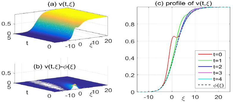
Figure 1: Case 1. $e<\frac{p}{d}\leq e^{2}$ with small time delay $r<\underline{r}$. (a) 3D-graphs of $v(t,\xi)$; (b) 3D-graphs of the error $v(t,\xi)-\phi(\xi)$; and (c) 2D-graphs of $v(t,\xi)$ at $t=0,1,2,3,4$ and the traveling wave $\phi(\xi)$.

Case 1. $e<\frac{p}{d}\leq e^{2}$ and $r<\underline{r}$ the solution converges to a monotone critical travelling wave $\phi(x+c^{*}t)$. We take $p=5$ and $r=0.2$. In this case, when $e<\frac{p}{d}\leq e^{2}$, the birth rate function $b(v)$ for $v\in[0,v_{+}]$ is non-monotone, where $v_{+}=\frac{1}{a}\ln\frac{p}{d}$. A direct calculation from (1.4), (1.5), and (3.39) gives $\underline{r}=0.4032979$, $c^{*}=5.1041202$, $\lambda_{*}=0.7801950$. Since $r<\underline{r}$, the critical wave $\phi(x+c^{*}t)$ is monotone. As numerically demonstrated in Figure 1, we can see that the solution behaves exactly like a monotone traveling wave, which are consistent with our stability Theorem 1.1.

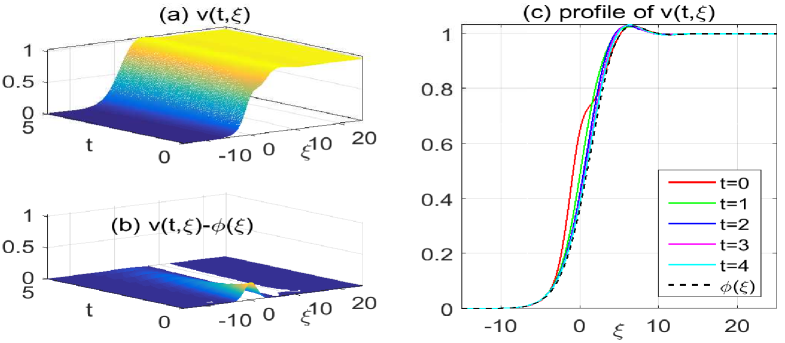
Figure 2: Case 2. $e<\frac{p}{d}\leq e^{2}$ with big time delay $r>\underline{r}$. (a) 3D-graphs of $v(t,\xi)$; (b) 3D-graphs of the error $v(t,\xi)-\phi(\xi)$; and (c) 2D-graphs of $v(t,\xi)$ at $t=0,1,2,3,4$ and the traveling wave $\phi(\xi)$.

Case 2. $e<\frac{p}{d}\leq e^{2}$ and $r>\underline{r}$ the solution converges to an oscillatory critical travelling wave $\phi(x+c^{*}t)$. We can choose $p=5$ and $r=2$. Similarly, we have $\underline{r}=0.4032979$, $c^{*}=1.3108958$, $\lambda_{*}=0.7548876$ from (1.4), (1.5), and (3.39). In this case, $r>\underline{r}$, the critical traveling wave may be oscillating. The numerical results are shown in Figure 2. Figure 2 shows that the solution $v(t,x)$ is oscillating, and it converges to the oscillatory critical traveling wave.

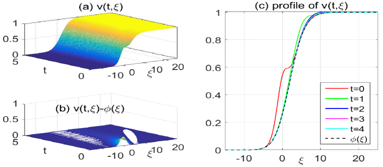
Figure 3: Case 3. $\frac{p}{d}>e^{2}$ with small time delay $r<\underline{r}$. (a) 3D-graphs of $v(t,\xi)$; (b) 3D-graphs of the error $v(t,\xi)-\phi(\xi)$; and (c) 2D-graphs of $v(t,\xi)$ at $t=0,1,2,3,4$ and the traveling wave $\phi(\xi)$.

Case 3. $\frac{p}{d}>e^{2}$ and $r<\underline{r}$ the solution converges to a monotone critical travelling wave $\phi(x+c^{*}t)$. We take $p=10$ and $r=0.2$ and get $\overline{r}=2.9304424$, $\underline{r}=0.2254235$, $c^{*}=7.1531405$, $\lambda_{*}=0.9315197$ from (1.4), (1.5), (3.38) and (3.39). Since $r<\underline{r}$, the critical wave $\phi(x+c^{*}t)$ is monotone. The numerical results showed in Figure 3 demonstrates that $v(t,x)$ behaves like the monotone critical traveling wave.

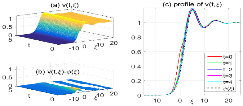
Figure 4: Case 4. $\frac{p}{d}>e^{2}$ with time delay $\underline{r}<r<\overline{r}$. (a) 3D-graphs of $v(t,\xi)$; (b) 3D-graphs of the error $v(t,\xi)-\phi(\xi)$; and (c) 2D-graphs of $v(t,\xi)$ at $t=0,1,2,3,4$ and the traveling wave $\phi(\xi)$.

Case 4. $\frac{p}{d}>e^{2}$ and $\underline{r}<r<\overline{r}$ the solution converges to an oscillatory critical travelling wave $\phi(x+c^{*}t)$. We take $p=10$ and $r=2$. A simple calculation from (1.4), (1.5), (3.38) and (3.39) gives $\overline{r}=2.9304424$, $\underline{r}=0.2254235$, $c^{*}=1.6178475$, $\lambda_{*}=0.8586847$. The numerical results given in Figure 4.

Acknowledgement. The research of S. Ji was supported by NSFC Grant No. 11701184, the Fundamental Research Funds for the Central Universities (No. 2017BQ109), and the China Postdoctoral Science Foundation (No. 2017M610517). The research of R. Huang was supported in part by NSFC Grants No. 11671155 and No. 11771155, NSF of Guangdong Grant No. 2016A030313418, and NSF of Guangzhou Grant No. 201607010207. The research of M. Mei was supported in part by NSERC Grant RGPIN 354724-16, and FRQNT Grant No. 2019-CO-256440. The research of J. Yin was supported in part by NSFC Grant No. 11771156.

References

[1]
F. Andreu-Vaillo, J. M. Mazn, J. D. Rossi, and J. J. Toledo-Melero,
Nonlocal Diffusion Problems,
Math. Surveys and Monographs, Vol. 165, Amer. Math. Soc., 2010.
[2]
C.-P. ,Cheng, W.-T. ,Li and Z.-C.,Wang
Asymptotic stability of traveling wavefronts in a delayed population model with stage structure on a two-dimensional spatial lattice.
Discrete Contin. Dyn. Syst. Ser. B
13(3): 559–575, 2010.
[3]
I-L. Chern, M. Mei, X. Yang, Q. Zhang,
Stability of non-monotone critical traveling waves for reaction-diffusion equations with time-delay,
J. Differential Equations
259(4):1503–1541,2015.
[4]
P. C. Fife and J. B. McLeod,
A phase plane discussion of convergence to travelling fronts
for nonlinear diffusion,
Arch. Ration. Mech. Anal.,
75: 281–314, 1980.
[5]
P. C. Fife,
Some nonclassical trends in parabolic and parabolic-like evolutions.
Trends in nonlinear analysis,
Springer, Berlin, 2003,153–191.
[6]
T. Gallay,
Local stability of critical fronts in nonlinear parabolic partial differential equations,
Nonlinearity,
7:741–764,1994.
[7]W. S. C. Gurney, S. P. Blythe, and R. M. Nisbet,
Nicholson’s blowflies revisited
Nature, 287 (1980), pp. 17–21.
[8]
S.A. Gourley, Y. Kuang,
Wavefronts and global stability in a time-delayed population model with stage structure,
Proc. R. Soc. Lond. Ser. A 459:1563–1579,2003.
[9]
S.A. Gourley, J. Wu,
Delayed nonlocal diffusive systems in biological invasion and disease spread,
in: Fields Inst. Commun., 48:137–200,2006.
[10]
R. Huang, M. Mei and Y. Wang,
Planar traveling waves for nonlocal dispersion equation with monostable nonlinearity
Discret. Contin. Dyn. Stst. A
32(10): 3621–3649, 2012.
[11]
R. Huang, M. Mei, K. J. Zhang and Q. F. Zhang,
Asymptotic stability of non-monotone traveling waves for time-delayed nonlocal dispersion equations.
Discret. Contin. Dyn. Stst.,
36(3):1331–1353, 2016.
[12]
V. Hutson, S. Martinez, K. Mischaikow, G.T. Vickers,
The evolutions of dispersal,
J. Math. Biol.,
47:483–517, 2003.
[13]
S.M. Ji, J.X. Yin, R. Huang.
Oscillatory traveling waves of ploytropic filtration equation with generalized
Fisher-KPP sources.
J. Math. Anal. Appl., 419:68–78, 2014.
[14]
D.Ya. Khusainov, A.F. Ivanov, I.V. Kovarzh,
Solution of one heat equation with delay,
Nonlinear Oscillasions,
12:260–282, 2009.
[15]
X. Liang and X.Q. Zhao.
Asymptotic speeds of spread and traveling waves for monotone
semiflows with applications.
Comm. Pure Appl. Math., 60:1-40, 2007.
[16]
C.-K. Lin, C.-T. Lin, Y. Lin, and M. Mei,
Exponential Stability of Nonmonotone Traveling Waves for Nicholson’s Blowflies Equation
SIAM J. Math. Anal., 46(2), 1053–1084, 2014.
[17] M. C. Mackey and L. Glass,
Oscillation and chaos in physiological control systems,
Science, 197(4300), 287-289, 1977.
[18]
M. Mei, C.-K. Lin, C.-T. Lin and J. W.-H. So,
Traveling wavefronts for time-delayed reactiondiffusion
equation. I. Local nonlinearity,
J. Differential Equations,
247:495–510, 2009.
[19]
M. Mei, C.-K. Lin, C.-T. Lin and J. W.-H. So,
Traveling wavefronts for time-delayed reactiondiffusion
equation. II. Nonlocal nonlinearity,
J. Differential Equations,
247:511–529,2009.
[20]
M. Mei, C. Ou, and X.Q. Zhao.
Global stability of monostable traveling waves for nonlocal
time-delayed reaction-diffusion equations.
SIAM J. Math. Anal., 42:2762–2790, 2010.
[21]
M. Mei, J. W.-H. So, M. Li, and S. Shen,
Asymptotic stability of traveling waves for the
Nicholson’s blowflies equation with diffusion,
Proc. Roy. Soc. Edinburgh Sect. A,
134:579–594,2004.
[22]
M. Mei and J. W.-H. So,
Stability of strong traveling waves for a nonlocal time-delayed
reaction-diffusion equation,
Proc. Roy. Soc. Edinburgh Sect. A, 138:551–568,2008.
[23]
M. Mei, Y. Wang,
Remark on stability of traveling waves for nonlocal Fisher-KPP equations,
Int. J. Numer. Anal. Model. Ser. B,
2:379-401,2011.
[24]
M. Mei and Y. S. Wong,
Novel stability results for traveling wavefronts in an age-structured
reaction-diffusion equations,
Math. Biosci. Engin.,
6:746–752, 2009.
[25]
M. Mei, K. Zhang and Q. Zhang,
Global stability of critical traveling waves with oscillations for
time-delayed reaction-diffusion equations.
preprint.
[26]
H. J. K. Moet,
A note on asymptotic behavior of solutions of the KPP equation,
SIAM J. Math. Anal., 10:728–732, 1979.
[27]
S. Pan, W.-T. Li and G. Lin,
Existence and stability of traveling wavefronts in a nonlocal diffusion equation with delay,
Nonlinear Anal.
72:3150–3158, 2010.
[28]
K. W. Schaaf,
Asymptotic behavior and traveling wave solutions for parabolic functional
differential equations,
Trans. Amer. Math. Soc., 302:587–615,1987.
[29]
W. Shen,
Traveling waves in time almost periodic structure governed by bistable nonlinearities,
I. Stability and uniqueness,
J. Differential Equations,
159:1–54, 1999.
[30]
H. L. Smith and X. Q. Zhao,
Global asymptotic stability of traveling waves in delayed reaction-diffusion equations,
SIAM J. Math. Anal., 31: 514–534,2000.
[31]
X. Tang, J. Shen,
Oscillation of delay differential equations with variable coefficients,
J. Math. Anal. Appl.
217:32–42, 1998.
[32]
H.R. Thieme and X.Q. Zhao,
Asymptotic speeds of spread and traveling waves for integral
equations and delayed reactioncdiffusion models.
J. Differential Equations,
195:430-470,
2003.
[33]
X. Wang,
Metastability and stability of patterns in a convolution model for phase
transitions,
J. Differential Equations,
183 434–461,2002.
[34]
Z.-C. Wang, W.-T. Li, and S. Ruan,
Existence and stability of traveling wave fronts in
reaction advection diffusion equations with nonlocal delay,
J. Differential Equations,
238:153–200,2008.
[35]
Y. Wu and X. Xing,
Stability of traveling waves with critical speeds for p-degree Fisher-type
equations,
Discrete Contin. Dyn. Syst.,
20:1123–1139, 2008.
[36]
T. Xu, S. Ji, M. Mei and J. Yin,
Traveling waves for time-delayed reaction diffusion equations with
degenerate diffusion,
preprint.
[37]
G.-B. Zhang,
Traveling waves in a nonlocal dispersal population model with
age-structure.
Nonlinear Anal. TMA ,74:5030–5047,2011.
[38]
G.-B. Zhang,
Non-monotone traveling waves and entire solutions for a delayed nonlocal dispersal equation,
Appl. Anal. 96 (2017) 1830?1866.
[39]
G.-B. Zhang and R. Ma,
Spreading speeds and traveling waves for a nonlocal dispersal equation
with convolution-type crossing-monostable nonlinearity,
Z. Ang. Math. Phys., 64:1643–1659,2013.
[40]
G.-B. Zhang, W.-T. Li and Z.-C. Wang
Spreading speeds and traveling waves for nonlocal dispersal equations with
degenerate monostable nonlinearity.
J. Differential Equations,
252:5096–5124 ,2012.