Fast likelihood evaluation for multivariate phylogenetic comparative methods: the PCMBase R package

Abstract

We introduce an R package, PCMBase, to rapidly calculate the likelihood for multivariate phylogenetic comparative methods. The package is not specific to particular models but offers the user the functionality to very easily implement a wide range of models where the transition along a branch is multivariate normal. We demonstrate the package’s possibilities on the now standard, multitrait Ornstein–Uhlenbeck process as well as the novel multivariate punctuated equilibrium model. The package can handle trees of various types (e.g. ultrametric, nonultrametric, polytomies, e.t.c.), as well as measurement error, missing measurements or non-existing traits for some of the species in the tree.

1 Introduction

Since Felsenstein (1985)’s work describing the independent contrasts algorithm, phylogenetic comparative methods (PCMs) have steadily been generalized with respect to available models and implementations of them. Following Felsenstein (1988)’s suggestion, Hansen (1997) described the Ornstein–Uhlenbeck (OU) process in the PCM setting. This led to the implementation of OU models in various packages such as ouch (Butler and King, 2004) or geiger (Harmon et al., 2008) to name a few, making it a standard model in the community alongside the Brownian motion (BM) process popularized in the community by Felsenstein (1985) but see also Edwards (1970); Lande (1976). For species being characterized by multiple traits, the multivariate OU processes was introduced by R packages such as ouch, slouch (Hansen et al., 2008), mvSLOUCH (Bartoszek et al., 2012), mvMORPH (Clavel et al., 2015), Rphylopars (Goolsby et al., 2016), again, to name a few. At the core of these methods, the likelihood of the model parameters and tree for given trait data is evaluated, meaning the probability density of the tip trait values given the parameters and tree is calculated.

From a statistical point of view, the development of phylogenetic comparative methods goes in two directions. The first direction is development of model classes beyond simple stochastic processes, such as BM and OU, and the second direction is the development of efficient likelihood evaluation methods. Considering the first direction, we briefly mention three recent proposals. Manceau et al. (2016) show (with implementation in RPANDA) that if one models the suite of traits by a linear stochastic differential equation (SDE, see the representation by Eq. (1) of Manceau et al., 2016) whose drift matrix (“deterministic part” of the SDE) is piecewise constant with respect to the phylogeny, and diffusion matrix (“random part”, sometimes referred to as “random drift part” in biological literature) does not depend on the trait, then the tip measurements are multivariate normal. The tip measurements’ mean vector and covariance matrix can be found by integrating (backwards along the tree) an appropriate collection of ordinary differential equations (ODEs), which in turn is required for the likelihood calculation. Landis et al. (2012); Duchen et al. (2017) went beyond the SDE world, represented through the equation,

$$\mathrm{d}\vec{X}_{t}=\mu(t,\vec{X}_{t})+\sigma(t,\vec{X}_{t})\mathrm{d}\vec{W}_{t},$$ (1)

where $\vec{W}_{t}$ is a standard multivariate Wiener process, into Lévy process models. These are highly relevant from a biological point of view as they allow for jumps in the trait at random time instances. Hence, they hold promise for attacking the longstanding question of whether “evolution is gradual or punctuated?”. Both approaches consider the transition densities, meaning the change of a trait between the start and the end of a branch, when quantifying trait evolution along a phylogeny. The third approach is to model the evolution of the traits’ density in time with a partial differential equation (PDE Boucher et al., 2018; Blomberg, 2017). E.g. in the simplest standard Wiener process case the PDEs are $\frac{\partial}{\partial t}f_{t}(x)=\frac{1}{2}\frac{\partial^{2}}{\partial x^{2}}f_{t}(x)$ with boundary condition $f_{0}(x)=\delta_{0}(x)$, i.e. Dirac $\delta$ at $0$.

The other direction is the development of efficient likelihood evaluation methods. Commonly, in PCMs, the model classes have the property that the joint distribution of the tip measurements is multivariate normal. Hence, there is a closed form for the likelihood—the multivariate normal density function, i.e. an algebraic expression in terms of the traits’ mean vector and the traits’ variance-covariance matrix $(\mathbf{V})$. Even though it is possible to obtain a conceptually simple equation, actually calculating the value of the likelihood is a computational challenge. If one has multiple correlated trait measurements per species, then $\mathbf{V}$ can have a very complicated formula (cf. Eqs (A.1, B.3, B.7) of Bartoszek et al., 2012). As Freckleton (2012) points out “First, the matrix has to be generated in the first place. This requires allocating enough memory to hold all of the entries of $\mathbf{V}$ and then initiating one traversal (i.e. successively visiting all the nodes) of the phylogeny per pair of species sharing an ancestor to measure the shared path lengths. Second $\mathbf{V}$ has to be inverted at one point in the analysis.”.

Hence, effort has been invested into reducing the memory and time complexity of the likelihood evaluation process. Inspired by Felsenstein (1973)’s approach, Freckleton (2012) proposed a linear (w.r.t. the number of tips of the phylogeny) way to obtain the likelihood for traits evolving as a Brownian motion. Freckleton (2012), further indicates that non–Brownian models can be quickly evaluated if one appropriately transforms the phylogeny. Then, Ho and Ané (2014) proposed a general method that takes advantage of the so–called $3$–point structure of the Brownian motion’s between–species–between–traits variance–covariance matrix (i.e. a matrix $\mathbf{S}$ has a $3$–point structure if it is symmetric, with non–negative entries and for all $i$, $j$, $k$ (possibly equal), the two smallest of $\mathbf{S}_{ij}$, $\mathbf{S}_{ik}$ and $\mathbf{S}_{jk}$ are equal Ho and Ané, 2014) and obtain the likelihood in linear (w.r.t. the number of tips of the phylogeny) time, without having to construct in quadratic time the matrix $\mathbf{V}$. Similarly, calculating the likelihood for non–Brownian models (like the univariate Ornstein–Uhlenbeck process) can be done in linear time, as long as their $\mathbf{V}$ satisfies a generalized $3$–point structure. Briefly, a covariance matrix satisfies the generalized $3$–point structure if there exist diagonal matrices $\mathbf{D}_{1}$ and $\mathbf{D}_{2}$ such that $\mathbf{D}_{1}\mathbf{V}\mathbf{D}_{2}$ satisfies the $3$–point structure. Goolsby et al. (2016) derives such a transformation to find the likelihood for traits under multivariate Ornstein–Uhlenbeck evolution in linear time. But in their implementation, only ultrametric trees and symmetric–positive–definite drift matrices are supported at the moment. For non–Gaussian models, a quasi–likelihood is defined and again the same approach (as long as the generalized $3$–point structure holds) can be used (Ho and Ané, 2014).

The speed–up for the Brownian motion’s $3$–point structure (or generalized 3-point structure) is based on the fact that the between–species–between–traits variance–covariance matrix has a nested structure. Therefore, appropriate linear algebra allows for rapid calculation of $\mathrm{det}(\mathbf{V})$ and quadratic forms like $\vec{x}\mathbf{V}^{-1}\vec{y}$ without the need to do the inversion $\mathbf{V}^{-1}$.

Even though linear–time likelihood evaluation based on the $3$–point structure is mathematically elegant, it is, due to the necessity of finding an appropriate transformation for non–Brownian motion, intrinsically complicated and may seem daunting for a non–algebraically oriented user or developer. FitzJohn (2012) indicated a probabilistically motivated way of quickly finding the likelihood (with implementation in the Diversitree R package). He noticed (in the Supporting Information), same as Pybus et al. (2012), that one can traverse the tree and successively integrate out the internal nodes. FitzJohn (2012)’s description was focused around the BM and univariate OU processes on ultrametric trees. Furthermore, FitzJohn (2012) writes that he proved correctness of his method for a three tip phylogeny and then for larger trees checked numerically.

The presence of two different approaches, namely the 3–point structure method and the tree traversal method, to quickly calculating the likelihood combined with a number of independent implementations, each with some given set of conditions, can easily cause confusion. In fact, it seems that this led Slater (2014) to write in his Correction (due to “$\ldots$ errors arose from use of branch length rescaling under the Ornstein–Uhlenbeck process, which I here show to be inappropriate for non–ultrametric trees”), that “$\ldots$, there is little, if any documentation in the literature or elsewhere highlighting that one of these approaches can be used while another cannot.”

In this paper we attempt to overcome the difficulties highlighted in the previous paragraph by proposing a fast method to obtain the likelihood which integrates over the internal node values. Our approach is appropriate for a large class of models, namely for all models where conditional on the ancestral trait, the descendant trait is normally distributed , the descendant’s expectation depends linearly on the ancestor, and the variance does not depend on the ancestral value. From a mathematical point of view, we provide an inductive proof of FitzJohn (2012)’s claim of method correctness for multiple traits and all kinds of trees. Pybus et al. (2012) point out that for such a method to work, it is needed “to keep track of partial” means and precisions. Here, we propose a very general, computationally effective, and developer friendly way of doing this by recursively updating the polynomial representation of the multivariate normal density function. In order to use our approach for some new model, one has to be able to calculate the variance of the transition along the branch, the shift in the mean along a branch, and the linear dependency (i.e. a matrix) on the ancestral state. Thus, in our probabilistic approach, one needs to understand only the dynamics of a single branch (lineage), something that is usually present at the model formulation stage. For OU based models, these quantities can be analytically calculated and we provide an implementation. For other models, a developer will have to do the calculations themselves, but this should be significantly less involved than finding the transformation for the $3$–point structure. In fact, for SDE–type models, Manceau et al. (2016) provide a general ODE method (Eqs. S2 and S3) to obtain the conditional mean and variance. Furthermore, our method can naturally handle measurement error (intra–species variability), missing data, and punctuated components (jumps), and allows for changes in parameters at arbitrary points along the tree. It is further appropriate for non–ultrametric, binary and multifurcating trees. All of such specifications can be provided by the user. In no case is any tree transformation required.

Our method encompasses a number of contemporary frameworks. In particular all OU type models (e.g. ouch, slouch, mvSLOUCH, mvMORPH) are covered by it. The RPANDA SDE framework (without interactions between lineages) is also covered as are current punctuated equilibrium models (OU along a branch with a normal jump, denoted JOU Bartoszek, 2014; Bokma, 2002). To the best of our knowledge, our implementation handles the widest class of BM– and OU–based models on the widest set of phylogenetic trees, including non–ultrametric and non–binary trees.

It is important to stress here one point about the presented methodology and accompanying package. Our aim is not to provide a complete inference framework. Rather we provide an efficient way to evaluate the likelihood for a phylogenetic comparative data set given a user–defined model. The user can then on top of our package optimize over the parameter space to find the maximum likelihood estimates or perform a Bayesian analysis. In Mitov et al. , we use the framework presented here to quantify the evolution of brain-body mass allometry in mammals.

The rest of the paper is organized as follows. In Section 2, we describe in detail our fast computational framework for phylogenetic comparative methods. In Section 3 we present the PCMBase R–package. Then, in Section 4 we describe how one can handle issues such as missing values, measurement error, punctuated components, trees with polytomies, as well as sequentially sampled data (such as fossil data) leading to non–ultrametric trees. Next, in Section 5, we discuss the standard Ornstein–Uhlenbeck setup and describe examples of model classes that are already provided within our package. Two widely used models—the multivariate Brownian motion and multivariate Ornstein–Uhlenbeck processes and a novel model— a multivariate Ornstein–Uhlenbeck model with jumps are provided. It should be noted that even though we call the BM and OU standard PCM models, our implementation goes beyond what can be usually found in implementations: First, we allow for non-ultrametric trees. Second, the only assumption that we make on the drift matrix (i.e. “deterministic part” of the SDE) is that it has to be eigendecomposable. This is in contrast to the assumption of this matrix being not only eigendecomposable but also non–singular (e.g. Rphylopars, mvMORPH, mvSLOUCH—but some exceptions to this are permitted). In Section 6 we report a technical validation test of the likelihood calculations and Section 7 is a discussion..

2 Fast phylogenetic computational framework

2.1 Phylogenetic notation

We assume that we are given a rooted phylogenetic tree $\mathbb{T}$ representing the ancestral relationship between $N$ species associated with the tips of the tree (fig. 1). We denote the tips of the tree by the numbers $1,\ldots,N$, the internal nodes by the numbers $N+1,\ldots,M-1$ (where $M$ is the total number of nodes in the tree) and the root-node by $0$. For any internal node $j$, we denote by $Desc(j)$ the set of its direct descendants. We denote by $\mathbb{T}_{j}$ the subtree rooted at node $j$. We denote by $t_{j}$ the known length of the branch in the tree leading to any tip or internal node $j$. By convention, we assume that time increases in the direction from the root to the tips of the tree, and $t_{j}$ are positive scalars.

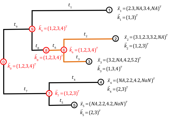
Figure 1: A phylogenetic tree with observations at the tips. Numbered circles in black indicate the tips with observed trait vectors $\vec{x}_{1},\ldots,\vec{x}_{N=5}$. Missing measurements are denoted as NA (Not Available), while non-existing traits are denoted as NaN (Not a Number). Numbered circles in red indicate the root, $0$, and the internal nodes $6,\ldots,9$, for which the trait vectors are unknown. The vectors, $\vec{k}_{i}$, denote the active coordinates for every node - for a tip-node these are all observed (neither NA nor NaN) coordinates; for an internal node, these are all the coordinates denoting traits that exist (are not NaN) for at least one of the tips descending from that node. The length of a branch leading to a tip or an internal node is known and denoted by $t_{i}$, $i=1,\ldots,9$. The change in branch color from black to orange at the internal node $8$ denotes the change to a different evolutionary regime. It is assumed that such a regime change occurs simultaneously for all traits.

The object of all phylogenetic models discussed here will be a suite of $k$ quantitative (real–valued) traits characterizing the $N$ species. Associated with each tip, $i$, there is a real $k$–vector, $\vec{x}_{i}$, of measured values for the $k$ traits. For some species, some trait measurements can be missing, reflecting two possible cases:

• the trait exists but was not measured for that species, denoted as NA (Not Available);

• the trait does not exist for that species denoted as NaN (Not a Number) (fig. 1).

We introduce algebraic notation that will hold for the rest of the paper. Scalars are denoted by lower case letters, e.g. $f$, vectors are indicated by the arrow notation, e.g. $\vec{\theta}$, while matrices are denoted as upper case bold letters, e.g. $\mathbf{H}$. An exception to this is $\mathbf{X}_{j}$, meaning the set of measurements at the tips descending from an internal node $j$ of the tree.

2.2 Phylogenetic models of continuous trait evolution

We assume that the trait values measured at the tips of the tree result from a continuous time continuous state–space Markovian process evolving on top of the branching pattern in the tree. By this we mean that along any given branch we have a trajectory following the law of the process. Then, at speciation, the process “splits” into two processes. Both processes inherit the last value of their parent process. After the branching points, there is no interaction between the processes. This entails that all the dependencies between the values at the tips come from the time between the origin of the tree and the most recent common ancestor for each pair of species. Exactly how this shared time of evolution is translated into a dependency depends on the assumed process. A widely used example of such trait process is the Ornstein–Uhlenbeck process illustrated in Fig. 2.

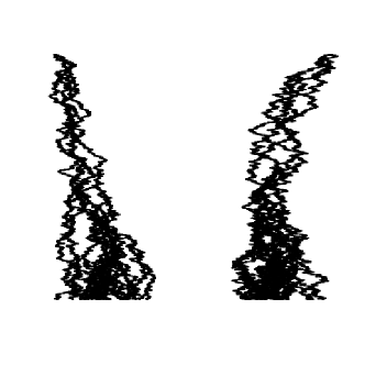
Figure 2: Simulation of a bivariate OU process on top of a pure birth tree with $30$ tips. The two traits are displayed on separate panels. The tree was simulated using the TreeSim package (Stadler, 2009, 2011), its height is $3.201$. The bivariate OU process was simulated using mvSLOUCH (Bartoszek et al., 2012) with parameters (matrices are represented by their rows) $\mathbf{H}=\{\{1,0.25\},\{0,2\}\},\leavevmode\nobreak\ \mathbf{\Sigma}_{x}=\{\{0.5,0.25\},\{0,0.5\}\},\leavevmode\nobreak\ \vec{\theta}=(1,-1)^{T}\leavevmode\nobreak\ \mathrm{and}\leavevmode\nobreak\ \vec{x}_{0}=(0,0)^{T}.$

Such stochastic processes are used as models of continuous trait evolution at the macro-evolutionary time scale, that is, when the time-units are in the order of hundreds to thousands of generations. Further in the text, we use the term “(trait evolutionary) model” to denote such kind of stochastic processes. We now turn to describing a family of models for which we will then provide an efficient way to calculate the likelihood of their parameters given the tree and the trait data observed at its tips.

2.3 The $\mathcal{G}_{LInv}$ family of models

The following definition specifies all requirements needed for a trait evolutionary model to be integrated within the fast computational framework:

Definition 1 (The $\mathcal{G}_{LInv}$ family).

We say that a trait evolutionary model belongs to the $\mathcal{G}_{LInv}$ family if it satisfies the following

1. after branching the traits evolve independently in all descending lineages,

2. the distribution of the trait vector at time $t$, $\vec{x}(t)$, conditional on the trait vector at time $s<t$, $\vec{x}(s)$, is Gaussian with the mean and variance satisfying

   1. $\operatorname{E}\left[\vec{x}(t)|\vec{x}(s)\right]=\vec{\omega}+\mathbf{\Phi}\vec{x}(s)$
      (the expectation is a linear function of the ancestral value),
      

   2. $\operatorname{Var}\left[\vec{x}(t)|\vec{x}(s)\right]=\mathbf{V}$
      (variance is invariant with respect to the ancestral value),

   for some vector $\vec{\omega}$ and matrices $\mathbf{\Phi}$, $\mathbf{V}$ which may depend on $s$ and $t$ but do not depend on the trait trajectory $\vec{x}(\cdot)$.

Later, in section 5, we show that the $\mathcal{G}_{LInv}$ family contains many well–known contemporary models such as BM, multivariate OU (where all traits are OU or some are BMs), BM or OU with normally distributed jumps. Now we derive an important property of the $\mathcal{G}_{LInv}$ family playing a key role for the fast likelihood calculation:

Theorem 1.

Let $\mathcal{M}$ be a trait model from the $\mathcal{G}_{LInv}$-family. Let $i$ be a tip or internal node and $j$ be its parent node in a tree $\mathbb{T}$, and let $\vec{x}_{i}\in\mathbb{R}^{k_{i}}$, $\vec{x}_{j}\in\mathbb{R}^{k_{j}}$ ($k_{i},k_{j}\in\mathbb{Z}^{+}$) be the trait–vectors at the nodes $i$ and $j$ under a realization of $\mathcal{M}$ on $\mathbb{T}$. Let $\vec{\omega}_{i}$, $\mathbf{\Phi}_{i}$ and $\mathbf{V}_{i}$ denote the terms $\vec{\omega}$, $\mathbf{\Phi}$ and $\mathbf{V}$ from definition 1 specific for node $i$. Then, the probability density function (pdf) of $\vec{x}_{i}$ conditioned on $\vec{x}_{j}$ can be expressed as the following exponential of a quadratic polynomial

$$pdf(\vec{x}_{i}|\vec{x}_{j})=\exp\bigg{[}\vec{x}_{i}^{T}\mathbf{A}_{i}\vec{x}_{i}+\vec{x}_{i}^{T}\vec{b}_{i}+\vec{x}_{j}^{T}\mathbf{C}_{i}\vec{x}_{j}+\vec{x}_{j}^{T}\vec{d}_{i}+\vec{x}_{j}^{T}\mathbf{E}_{i}\vec{x}_{i}+f_{i}\bigg{]},$$ (2)

where $\mathbf{A}_{i}$ is a symmetric negative-definite matrix, and all of the terms $\mathbf{A}_{i}$, $\vec{b}_{i}$, $\mathbf{C}_{i}$, $\vec{d}_{i}$, $\mathbf{E}_{i}$, $f_{i}$ are constants with respect to $\vec{x}_{j}$, specified by the equations:

$$\begin{array}[]{rcl}\mathbf{A}_{i}&=&-\frac{1}{2}\mathbf{V}_{i}^{-1}\in\mathbb{R}^{k_{i}\times k_{i}}\\ \vec{b}_{i}&=&\mathbf{V}_{i}^{-1}\vec{\omega}_{i}\in\mathbb{R}^{k_{i}}\\ \mathbf{C}_{i}&=&-\frac{1}{2}\mathbf{\Phi}_{i}^{T}\mathbf{V}_{i}^{-1}\mathbf{\Phi}_{i}\in\mathbb{R}^{k_{j}\times k_{j}}\\ \vec{d}_{i}&=&-\mathbf{\Phi}_{i}^{T}\mathbf{V}_{i}^{-1}\vec{\omega}_{i}\in\mathbb{R}^{k_{j}}\\ \mathbf{E}_{i}&=&\mathbf{\Phi}_{i}^{T}\mathbf{V}_{i}^{-1}\in\mathbb{R}^{k_{j}\times k_{i}}\\ f_{i}&=&-\frac{1}{2}\vec{\omega}_{i}^{T}\mathbf{V}_{i}^{-1}\vec{\omega}_{i}-\frac{k_{i}}{2}\log\left(2\pi\right)-\frac{1}{2}\log|\mathbf{V}_{i}|\in\mathbb{R}.\end{array}$$ (3)

Proof.

Substituting $\vec{\omega}_{i}+\mathbf{\Phi}_{i}\vec{x}_{j}$ and $\mathbf{V}_{i}$ for the mean and variance in the formula for the pdf of a multivariate Gaussian distribution, we obtain:

$$pdf(\vec{x}_{i}|\vec{x}_{j})=\exp\bigg{[}-\frac{1}{2}\left(\vec{x}_{i}-\left(\vec{\omega}_{i}+\mathbf{\Phi}_{i}\vec{x}_{j}\right)\right)^{T}\mathbf{V}_{i}^{-1}\left(\vec{x}_{i}-\left(\vec{\omega}_{i}+\mathbf{\Phi}_{i}\vec{x}_{j}\right)\right)-\frac{k_{i}}{2}\log\left(2\pi\right)-\frac{1}{2}\log|\mathbf{V}_{i}|\bigg{]}$$ (4)

By expanding and reordering the terms in parentheses, Eq. (4) can be rewritten as

$$\begin{array}[]{llll}pdf(\vec{x}_{i}|\vec{x}_{j})&=&\exp\bigg{[}&\vec{x}_{i}^{T}\big{(}-\frac{1}{2}\mathbf{V}_{i}^{-1}\big{)}\vec{x}_{i}+\\ &&&\vec{x}_{i}^{T}\big{(}\mathbf{V}_{i}^{-1}\vec{\omega}_{i}\big{)}+\\ &&&\vec{x}_{j}^{T}\big{(}-\frac{1}{2}\mathbf{\Phi}_{i}^{T}\mathbf{V}_{i}^{-1}\mathbf{\Phi}_{i}\big{)}\vec{x}_{j}+\\ &&&\vec{x}_{j}^{T}\big{(}-\mathbf{\Phi}_{i}^{T}\mathbf{V}_{i}^{-1}\vec{\omega}_{i}\big{)}+\\ &&&\vec{x}_{j}^{T}\big{(}\mathbf{\Phi}_{i}^{T}\mathbf{V}_{i}^{-1}\big{)}\vec{x}_{i}+\\ &&&\big{(}-\frac{1}{2}\vec{\omega}_{i}^{T}\mathbf{V}_{i}^{-1}\vec{\omega}_{i}-\frac{k_{i}}{2}\log\left(2\pi\right)-\frac{1}{2}\log|\mathbf{V}_{i}|\big{)}\bigg{]}.\end{array}$$ (5)

We can see the correspondence with the quadratic forms $\vec{x}_{i}^{T}(\ldots)\vec{x}_{i}$, $\vec{x}_{j}^{T}(\ldots)\vec{x}_{j}$ and the other terms in Eq. (2). Equation (3) follows immediately. Furthermore, $\mathbf{A}_{i}$ is a symmetric negative–definite matrix, because $\mathbf{V}_{i}$ is a symmetric positive–definite matrix as it is a variance–covariance matrix. Finally, all of the terms $\mathbf{A}_{i}$, $\vec{b}_{i}$, $\mathbf{C}_{i}$, $\vec{d}_{i}$, $\mathbf{E}_{i}$, $f_{i}$ are constant with respect to $\vec{x}_{j}$, because they are functions of $\vec{\omega}_{i}$, $\mathbf{\Phi}_{i}$ and $\mathbf{V}_{i}$ which are constants with respect to $\vec{x}_{j}$ by Def. 1. ∎

2.4 Calculating the likelihood of $\mathcal{G}_{LInv}$-models

Let $\mathcal{M}$ be a trait evolutionary model realized on a tree $\mathbb{T}$ and $\Theta$ denotes the parameters of $\mathcal{M}$. The likelihood of $\mathcal{M}$ for given trait data $\mathbf{X}$ associated with the tips of $\mathbb{T}$ is defined as the function $\ell(\Theta)=pdf(\mathbf{X}|\mathbb{T},\Theta)$. The representation of Eq. (2) allows for linear (in terms of the number of tips, $N$) calculation of the likelihood of any trait model in the $\mathcal{G}_{LInv}$-family, given a phylogeny and measured data at its tips. This follows from the next theorem.

Theorem 2.

Let $\mathcal{M}$ be a trait evolutionary model from the $\mathcal{G}_{LInv}$-family and $\mathbb{T}$ be a phylogenetic tree. Let $\Theta$ be the parameters of $\mathcal{M}$. For the root (0) or any internal node $j$ in $\mathbb{T}$, there exists a $k_{j}\times k_{j}$ matrix $\mathbf{L}_{j}$, a $k_{j}$–vector $\vec{m}_{j}$ and a scalar $r_{j}$, such that the likelihood of $\mathcal{M}$ for the data $\mathbf{X}_{j}$, conditioned on $\vec{x}_{j}\in\mathbb{R}^{k_{j}}$ and $\mathbb{T}$ is expressed as:

$$pdf(\mathbf{X}_{j}|\vec{x}_{j},\mathbb{T},\Theta)=\exp\left(\vec{x}_{j}^{T}\mathbf{L}_{j}\vec{x}_{j}+\vec{x}_{j}^{T}\vec{m}_{j}+r_{j}\right).$$ (6)

The parameters $\mathbf{L}_{j}$, $\vec{m}_{j}$, $r_{j}$ are functions of $\Theta$, the observed data $\mathbf{X}_{j}$, and the tree $\mathbb{T}$, namely, equations 9, 10, and 11.

Proof.

Following condition 1 of definition 1 we can factorize the conditional likelihood at any internal or root node $j$. Splitting $Desc(j)$, i.e. the set of nodes descending from node $j$, into tips and non–tips, denoted as $Desc(j)\cap\{1,...,N\}$ and $Desc(j)\setminus\{1,...,N\}$, we can write:

$$\begin{array}[]{rcl}pdf(\mathbf{X}_{j}|\vec{x}_{j},\mathbb{T},\Theta)&=&\left(\prod\limits_{i\in Desc(j)\cap\{1,...,N\}}pdf(\vec{x}_{i}|\vec{x}_{j},\mathbb{T},\Theta)\right)\times\\ &&\left(\prod\limits_{i\in Desc(j)\setminus\{1,...,N\}}\bigintss_{\mathbb{R}^{k}_{j}}pdf(\vec{x}_{i}|\vec{x}_{j},\mathbb{T},\Theta)\times pdf(\mathbf{X}_{i}|\vec{x}_{i},\mathbb{T},\Theta)\mathrm{d}\vec{x}_{i}\right).\end{array}$$ (7)

We first prove the Theorem for nodes where all descendants are tips. If all descendants of $j$ are tips (e.g. nodes 6 and 7 on Fig. 1), then, according to Eq. (2)

$$\begin{array}[]{rcl}pdf(\mathbf{X}_{j}|\vec{x}_{j},\mathbb{T},\Theta)&=&\prod\limits_{i\in Desc(j)}pdf(\vec{x}_{i}|\vec{x}_{j},\mathbb{T},\Theta)\\ &=&\exp\left(\sum\limits_{i\in Desc(j)}\vec{x}_{i}^{T}\mathbf{A}_{i}\vec{x}_{i}+\vec{x}_{i}^{T}\vec{b}_{i}+\vec{x}_{j}^{T}\mathbf{C}_{i}\vec{x}_{j}+\vec{x}_{j}^{T}\vec{d}_{i}+\vec{x}_{j}^{T}\mathbf{E}_{i}\vec{x}_{i}+f_{i}\right),\end{array}$$

resulting in

$$pdf(\mathbf{X}_{j}|\vec{x}_{j},\mathbb{T},\Theta)=\exp\left(\vec{x}_{j}^{T}(\sum\limits_{i\in Desc(j)}\mathbf{C}_{i})\vec{x}_{j}+\vec{x}_{j}^{T}(\sum\limits_{i\in Desc(j)}\vec{d}_{i}+\mathbf{E}_{i}\vec{x}_{i})+\sum\limits_{i\in Desc(j)}\vec{x}_{i}^{T}\mathbf{A}_{i}\vec{x}_{i}+\vec{x}_{i}^{T}\vec{b}_{i}+f_{i}\right)$$ (8)

Then, to obtain the representation from Eq. (6), we denote:

$$\begin{array}[]{rcl}\mathbf{L}_{j}&=&\sum\limits_{i\in Desc(j)}\mathbf{C}_{i}\\ \vec{m}_{j}&=&\sum\limits_{i\in Desc(j)}\vec{d}_{i}+\mathbf{E}_{i}\vec{x}_{i}\\ r_{j}&=&\sum\limits_{i\in Desc(j)}\vec{x}_{i}^{T}\mathbf{A}_{i}\vec{x}_{i}+\vec{x}_{i}^{T}\vec{b}_{i}+f_{i}\end{array}$$ (9)

If not all of $Desc(j)$ are tips, then, for the descendants which are tips, we define:

$$\begin{array}[]{rcl}\mathbf{L}_{j}^{tips}&=&\sum\limits_{i\in Desc(j)\cap\{1,...,N\}}\mathbf{C}_{i}\\ \vec{m}_{j}^{tips}&=&\sum\limits_{i\in Desc(j)\cap\{1,...,N\}}\vec{d}_{i}+\mathbf{E}_{i}\vec{x}_{i}\\ r_{j}^{tips}&=&\sum\limits_{i\in Desc(j)\cap\{1,...,N\}}\vec{x}_{i}^{T}\mathbf{A}_{i}\vec{x}_{i}+\vec{x}_{i}^{T}\vec{b}_{i}+f_{i}\end{array}$$ (10)

We perform mathematical induction to prove the Theorem for all nodes. We need to show that Eq. (6) holds for each non-tip descendant of $j$, that is, for each $i\in Desc(j)\setminus\{1,...,N\}$ there exists a $k_{i}\times k_{i}$ matrix $\mathbf{L}_{i}$, a $k_{i}$–vector $\vec{m}_{i}$ and a scalar $r_{i}$ such that $pdf(\mathbf{X}_{i}|\vec{x}_{i},\mathbb{T},\Theta)=\exp(\vec{x}_{i}^{T}\mathbf{L}_{i}\vec{x}_{i}+\vec{x}_{i}^{T}\vec{m}_{i}+r_{i})$. We proved the induction base case, namely, we proved above that the Eq. (6) holds for all nodes which have only tip–descendants. Then, the induction hypothesis is that for an internal node $j$, the statement of the theorem has been proven for all $i\in Desc(j)$. Now in the inductive step using Eq. (2) and the induction hypothesis, we can write the integral in Eq. (7) as

$$\int_{\mathbb{R}^{k_{i}}}pdf(\vec{x}_{i}|\vec{x}_{j},\mathbb{T},\Theta)\times pdf(\mathbf{X}_{i}|\vec{x}_{i},\mathbb{T},\Theta)\mathrm{d}\vec{x}_{i}\\ =\int_{\mathbb{R}^{k_{i}}}\exp\left(\vec{x}_{i}^{T}\mathbf{A}_{i}\vec{x}_{i}+\vec{x}_{i}^{T}\vec{b}_{i}+\vec{x}_{j}^{T}\mathbf{C}_{i}\vec{x}_{j}+\vec{x}_{j}^{T}\vec{d}_{i}+\vec{x}_{j}^{T}\mathbf{E}_{i}\vec{x}_{i}+f_{i}+\vec{x}_{i}^{T}\mathbf{L}_{i}\vec{x}_{i}+\vec{x}_{i}^{T}\vec{m}_{i}+r_{i}\right)\mathrm{d}\vec{x}_{i}\\ =\exp\left(\vec{x}_{j}^{T}\mathbf{C}_{i}\vec{x}_{j}+\vec{x}_{j}^{T}\vec{d}_{i}+f_{i}+r_{i}\right)\times\boxed{\int_{\mathbb{R}^{k_{i}}}\exp\left(\vec{x}_{i}^{T}(\mathbf{A}_{i}+\mathbf{L}_{i})\vec{x}_{i}+\vec{x}_{i}^{T}(\vec{b}_{i}+\vec{m}_{i}+\mathbf{E}_{i}^{T}\vec{x}_{j})\right)\mathrm{d}\vec{x}_{i}}\\ \stackrel{{\scriptstyle\bigstar}}{{=}}\exp\left(\vec{x}_{j}^{T}\mathbf{C}_{i}\vec{x}_{j}+\vec{x}_{j}^{T}\vec{d}_{i}+f_{i}+r_{i}\right)\left(\sqrt{2\pi}\right)^{k_{i}}\boxed{\left(\sqrt{|(-2)\left(\mathbf{A}_{i}+\mathbf{L}_{i}\right)|}\right)^{-1}}\\ \times\exp\left(-(1/4)\left(\vec{b}_{i}+\vec{m}_{i}+\mathbf{E}_{i}^{T}\vec{x}_{j}\right)^{T}\left(\mathbf{A}_{i}+\mathbf{L}_{i}\right)^{-1}\left(\vec{b}_{i}+\vec{m}_{i}+\mathbf{E}_{i}^{T}\vec{x}_{j}\right)\right)$$

$$=\exp\left(\vec{x}_{j}^{T}\mathbf{C}_{i}\vec{x}_{j}+\vec{x}_{j}^{T}\vec{d}_{i}+f_{i}+r_{i}\right)\left(\sqrt{2\pi}\right)^{k_{i}}\left(\sqrt{|(-2)\left(\mathbf{A}_{i}+\mathbf{L}_{i}\right)|}\right)^{-1}\\ \times\exp\left(-(1/4)\left(\vec{b}_{i}+\vec{m}_{i}\right)^{T}\left(\mathbf{A}_{i}+\mathbf{L}_{i}\right)^{-1}\left(\vec{b}_{i}+\vec{m}_{i}\right)-(1/2)\vec{x}_{j}^{T}\mathbf{E}_{i}\left(\mathbf{A}_{i}+\mathbf{L}_{i}\right)^{-1}\left(\vec{b}_{i}+\vec{m}_{i}\right)\right.\\ \left.-(1/4)\vec{x}_{j}^{T}\mathbf{E}_{i}\left(\mathbf{A}_{i}+\mathbf{L}_{i}\right)^{-1}\mathbf{E}_{i}^{T}\vec{x}_{j}\right)\\ =\exp\left(\vec{x}_{j}^{T}\left(\mathbf{C}_{i}-(1/4)\mathbf{E}_{i}\left(\mathbf{A}_{i}+\mathbf{L}_{i}\right)^{-1}\mathbf{E}_{i}^{T}\right)\vec{x}_{j}+\vec{x}_{j}^{T}\left(\vec{d}_{i}-(1/2)\mathbf{E}_{i}\left(\mathbf{A}_{i}+\mathbf{L}_{i}\right)^{-1}\left(\vec{b}_{i}+\vec{m}_{i}\right)\right)\right.\\ \left.+f_{i}+r_{i}+(k_{i}/2)\log(2\pi)-(1/2)\log(|(-2)\left(\mathbf{A}_{i}+\mathbf{L}_{i}\right)|)-(1/4)\left(\vec{b}_{i}+\vec{m}_{i}\right)^{T}\left(\mathbf{A}_{i}+\mathbf{L}_{i}\right)^{-1}\left(\vec{b}_{i}+\vec{m}_{i}\right)\right)$$

We can then see that for a non–tip node we can define

$$\begin{array}[]{rcl}\mathbf{L}_{j}^{non-tips}&=&\sum\limits_{i\in Desc(j)\setminus\{1,...,N\}}\left(\mathbf{C}_{i}-(1/4)\mathbf{E}_{i}\left(\mathbf{A}_{i}+\mathbf{L}_{i}\right)^{-1}\mathbf{E}_{i}^{T}\right)\\ \vec{m}_{j}^{non-tips}&=&\sum\limits_{i\in Desc(j)\setminus\{1,...,N\}}\left(\vec{d}_{i}-(1/2)\mathbf{E}_{i}\left(\mathbf{A}_{i}+\mathbf{L}_{i}\right)^{-1}\left(\vec{b}_{i}+\vec{m}_{i}\right)\right)\\ r_{j}^{non-tips}&=&\sum\limits_{i\in Desc(j)\setminus\{1,...,N\}}\left(f_{i}+r_{i}+(k_{i}/2)\log(2\pi)-(1/2)\log(|(-2)\left(\mathbf{A}_{i}+\mathbf{L}_{i}\right)|)\right.\\ &&\left.-(1/4)\left(\vec{b}_{i}+\vec{m}_{i}\right)^{T}\left(\mathbf{A}_{i}+\mathbf{L}_{i}\right)^{-1}\left(\vec{b}_{i}+\vec{m}_{i}\right)\right).\end{array}$$ (11)

The representation of $\mathbf{L}_{j}^{non-tips}$, $\vec{m}_{j}^{non-tips}$ and $r_{j}^{non-tips}$ in Eq. (11) immediately entails the existence of the $\mathbf{L}_{j}$, $\vec{m}_{j}$ and $r_{j}$ elements in Eq. (6) for internal or root nodes $j$, hence we obtain the claimed polynomial form in the inductive step and in consequence the theorem. ∎

The inductive proof of Thm. 2 defines a pruning–wise procedure for calculating $\mathbf{L}_{0}$, $\vec{m}_{0}$ and $r_{0}$ (we remind that $0$ stands for the root of the tree). In order to calculate the likelihood of the tree conditioned on $\vec{x}_{0}$, we use Thm 2 with $j$ being the root node. In order to be able to calculate the full likelihood, it now only remains to specify how to deal with the unknown trait value at the root of the tree, $\vec{x}_{0}$, i.e. the ancestral state. This is an implementation detail up to the user. Our implementation of the various models provided (sections 3 and 5) with the PCMbase package allow for maximizing the polynomial with respect to $\vec{x}_{0}$ or for treating it as a free parameter (like the elements of the parameter set $\Theta$) that the user provides.

2.5 Scope of the framework

We now investigate if there are other trait evolutionary models, beyond the $\mathcal{G}_{LInv}$–family, for which the likelihood can be calculated using the same recursive formulae, Eqs. (9), (10), and (11) First, since we calculate the likelihood in a recursive pruning fashion, we assume that evolution is independent across branches, meaning condition $1$ is a necessary condition. In Theorem 3, we prove that the condition $2$ in Def. 1 is also a necessary condition. In other words, we show that if the likelihood can be calculated via recursion based on Eqs. (3), (8), then the model is in the $\mathcal{G}_{LInv}$–family.

Theorem 3.

Let $\mathcal{M}$ be a trait model satisfying condition $1$ of Def. 1 and realized on a tree $\mathbb{T}$. If for every parent–child pair of nodes $<j,i>$ in $\mathbb{T}$, the trait–vector $\vec{x}_{i}\in\mathbb{R}^{k_{i}}$ ($k_{i}\in\mathbb{Z}^{+}$) has non–zero support on the whole of $\mathbb{R}^{k_{i}}$ and there exist a symmetric negative–definite matrix $\mathbf{A}_{i}\in\mathbb{R}^{k_{i}\times k_{i}}$ and components $\vec{b}_{i}\in\mathbb{R}^{k_{i}}$, $\mathbf{C}_{i}\in\mathbb{R}^{k_{j}\times k_{j}}$, $\vec{d}_{i}\in\mathbb{R}^{k_{j}}$, $\mathbf{E}_{i}\in\mathbb{R}^{k_{j}\times k_{i}}$, $f_{i}\in\mathbb{R}$, such that, for any vector of values at the parent node, $\vec{x}_{j}\in\mathbb{R}^{k_{j}}$ ($k_{j}\in\mathbb{Z}^{+}$), the pdf of $\vec{x}_{i}$ conditional on $\vec{x}_{j}$ can be expressed by Eq. (2), then $\mathcal{M}$ belongs to the ${G}_{LInv}$–family and the terms $\vec{\omega}_{i}$, $\mathbf{\Phi}_{i}$ and $\mathbf{V}_{i}$ denoting the terms $\vec{\omega}$, $\mathbf{\Phi}$ and $\mathbf{V}$ from Def. 1 specific for node $i$ satisfy Eq. (3).

Proof.

We rearrange the terms on the right–hand side of Eq. (2) as follows

$$\begin{array}[]{l}pdf(\vec{x}_{i}|\vec{x}_{j})=\exp\bigg{[}\vec{x}_{i}^{T}\mathbf{A}_{i}\vec{x}_{i}-2\vec{x}_{i}^{T}\mathbf{A}_{i}\left((-\frac{1}{2}\mathbf{A}_{i}^{-1})\left(\vec{b}_{i}+\mathbf{E}_{i}^{T}\vec{x}_{j}\right)\right)+\left(\vec{x}_{j}^{T}\mathbf{C}_{i}\vec{x}_{j}+\vec{x}_{j}^{T}\vec{d}_{i}+f_{i}\right)\bigg{]}\\ =\exp\bigg{[}\left(\vec{x}_{i}+\frac{1}{2}\mathbf{A}_{i}^{-1}\left(\vec{b}_{i}+\mathbf{E}_{i}^{T}\vec{x}_{j}\right)\right)^{T}\mathbf{A}_{i}\left(\vec{x}_{i}+\frac{1}{2}\mathbf{A}_{i}^{-1}\left(\vec{b}_{i}+\mathbf{E}_{i}^{T}\vec{x}_{j}\right)\right)-\frac{1}{4}\left(\vec{b}_{i}+\mathbf{E}_{i}^{T}\vec{x}_{j}\right)^{T}\mathbf{A}_{i}^{-1}\left(\vec{b}_{i}+\mathbf{E}_{i}^{T}\vec{x}_{j}\right)\\ +\left(\vec{x}_{j}^{T}\mathbf{C}_{i}\vec{x}_{j}+\vec{x}_{j}^{T}\vec{d}_{i}+f_{i}\right)\bigg{]}.\end{array}$$ (12)

As the above is by definition a density on $\mathbb{R}^{k_{i}}$, integrating over $\vec{x}_{i}$ equals $1$. Hence, after taking all constants with respect to $\vec{x}_{i}$ out of the integral and multiplying/dividing the integral by the constant $(\sqrt{|2\pi(-2)\mathbf{A}_{i}|})^{-1}$, we obtain:

$$\begin{array}[]{lcl}1&=&\underbrace{\bigintsss\limits_{\mathbb{R}^{k_{i}}}\frac{1}{\sqrt{|2\pi(-2)\mathbf{A}_{i}|}}\exp\bigg{[}-\frac{1}{2}\left(\vec{x}_{i}+\frac{1}{2}\mathbf{A}_{i}^{-1}\left(\vec{b}_{i}+\mathbf{E}_{i}^{T}\vec{x}_{j}\right)\right)^{T}\left(-2\mathbf{A}_{i}\right)\left(\vec{x}_{i}+\frac{1}{2}\mathbf{A}_{i}^{-1}\left(\vec{b}_{i}+\mathbf{E}_{i}^{T}\vec{x}_{j}\right)\right)\bigg{]}\mathrm{d}\vec{x}_{i}}_{=1}\\ &&\times\sqrt{|2\pi(-2)\mathbf{A}_{i}|}\times\exp\bigg{[}-\frac{1}{4}\left(\vec{b}_{i}+\mathbf{E}_{i}^{T}\vec{x}_{j}\right)^{T}\mathbf{A}_{i}^{-1}\left(\vec{b}_{i}+\mathbf{E}_{i}^{T}\vec{x}_{j}\right)+\left(\vec{x}_{j}^{T}\mathbf{C}_{i}\vec{x}_{j}+\vec{x}_{j}^{T}\vec{d}_{i}+f_{i}\right)\bigg{]}\\ &=&\exp\bigg{[}\frac{k_{i}}{2}\log(2\pi)+\frac{1}{2}\log|(-2)\mathbf{A}_{i}|\bigg{]}\times\exp\bigg{[}-\frac{1}{4}\left(\vec{b}_{i}+\mathbf{E}_{i}^{T}\vec{x}_{j}\right)^{T}\mathbf{A}_{i}^{-1}\left(\vec{b}_{i}+\mathbf{E}_{i}^{T}\vec{x}_{j}\right)+\left(\vec{x}_{j}^{T}\mathbf{C}_{i}\vec{x}_{j}+\vec{x}_{j}^{T}\vec{d}_{i}+f_{i}\right)\bigg{]}\\ &=&\exp\bigg{[}\vec{x}_{j}^{T}\left(\mathbf{C}_{i}-\frac{1}{4}\mathbf{E}_{i}\mathbf{A}_{i}^{-1}\mathbf{E}_{i}^{T}\right)\vec{x}_{j}+\vec{x}_{j}^{T}\left(\vec{d}_{i}-\frac{1}{2}\mathbf{E}_{i}\mathbf{A}_{i}^{-1}\vec{b}_{i}\right)+f_{i}+\frac{k_{i}}{2}\log(2\pi)+\frac{1}{2}\log\big{(}|(-2)\mathbf{A}_{i}|\big{)}-\frac{1}{4}\vec{b}_{i}^{T}\mathbf{A}_{i}^{-1}\vec{b}_{i}\bigg{]}.\end{array}$$ (13)

When calculating the integral in Eq. (13) above, we have used the fact that the matrix $(-2)\mathbf{A}_{i}$ is a symmetric positive–definite matrix as it is the negative of the symmetric negative–definite matrix $2\mathbf{A}_{i}$. Hence, the so constructed function below the integral in Eq. (13) is a $k_{i}$-variate Gaussian pdf with mean vector $-\frac{1}{2}\mathbf{A}_{i}^{-1}\left(\vec{b}_{i}+\mathbf{E}_{i}^{T}\vec{x}_{j}\right)$ and variance–covariance matrix $(-2)\mathbf{A}_{i}$.

By definition, $\mathbf{A}_{i}$, $\vec{b}_{i}$, $\mathbf{C}_{i}$, $\vec{d}_{i}$, $\mathbf{E}_{i}$, $f_{i}$ are constant with respect to $\vec{x}_{j}$. Therefore, Eq. 13 has to hold for all $\vec{x}_{j}$. This implies the relationships:

$$\begin{array}[]{rcl}\mathbf{C}_{i}&=&\mathbf{E}_{i}\mathbf{A}_{i}^{-T}\mathbf{E}_{i}^{T},\\ \vec{d}_{i}&=&2\mathbf{E}_{i}\mathbf{A}_{i}^{-1}\vec{b}_{i},\\ f_{i}&=&\frac{1}{4}b_{i}^{T}\mathbf{A}_{i}^{-1}b_{i}-\frac{k_{i}}{2}\log(2\pi)-\frac{1}{2}\log\big{(}|(-2)\mathbf{A}_{i}|\big{)}.\end{array}$$ (14)

Next, we define $\mathbf{V}_{i}:=(-\frac{1}{2})\mathbf{A}_{i}^{-1}$, $\vec{\omega}_{i}:=(-\frac{1}{2})\mathbf{A}_{i}^{-1}\vec{b}_{i}$ and $\mathbf{\Phi}_{i}:=(-\frac{1}{2})\mathbf{A}_{i}^{-1}\mathbf{E}_{i}^{T}$. Since $\mathbf{A}_{i}$ is symmetric negative–definite, $\mathbf{V}_{i}$ is symmetric positive–definite. Combining the above three definitions with Eq. (14) and expressing $\mathbf{A}_{i}$, $\vec{b}_{i}$, $\mathbf{C}_{i}$, $\vec{d}_{i}$, $\mathbf{E}_{i}$, $f_{i}$ in terms of $\vec{\omega}_{i}$, $\mathbf{\Phi}_{i}$ and $\mathbf{V}_{i}$, we obtain again Eq. (3). Then, we can follow the equivalences in backward direction (Eqs. (3)$\rightarrow$(5)$\rightarrow$(4)) to prove that the pdf defined in Eq. (2) is equivalent to the Gaussian pdf defined in terms of $\vec{\omega}_{i}$, $\mathbf{\Phi}_{i}$ and $\mathbf{V}_{i}$, Eq. (4). We note also that $\vec{\omega}_{i}$, $\mathbf{\Phi}_{i}$ and $\mathbf{V}_{i}$ defined above are constant with respect to $\vec{x}_{j}$, because they are defined in terms of $\mathbf{A}_{i}$, $\vec{b}_{i}$ and $\mathbf{E}_{i}$, which are constant with respect to $\vec{x}_{j}$ by definition. With that we proved condition $2$ of Def. 1. Since $\mathcal{M}$ satisfies condition $1$ of Def. 1 by the first sentence in the Theorem, it follows that $\mathcal{M}$ belongs to the $\mathcal{G}_{LInv}$–family. ∎

Remark 1.

In Eq. (2), it suffices to consider symmetric negative–definite matrices $\mathbf{A}$ only. We remind that, by definition, a matrix $\mathbf{A}$ is negative–definite iff $\vec{x}^{T}\mathbf{A}\vec{x}<0$ for every $\vec{x}\neq\vec{0}$. Considering non–symmetric negative–definite matrices $\mathbf{A}$ does not extend the family of pdfs represented by Eq. (2). In particular, for any square negative–definite matrix $\mathbf{Q}$, and (of appropriate size) vector $\vec{u}$, it holds that $\vec{u}^{T}\mathbf{Q}\vec{u}=\vec{u}^{T}\big{[}\frac{1}{2}(\mathbf{Q}+\mathbf{Q}^{T})\big{]}\vec{u}$ and the matrix $\big{[}\frac{1}{2}(\mathbf{Q}+\mathbf{Q}^{T})\big{]}$ is symmetric negative–definite. Hence if one took in Eq. (2) a non–symmetric $\mathbf{A}$, then the value of the pdf would be the same as if one had taken the symmetric negative–definite matrix $\big{[}\frac{1}{2}(\mathbf{A}+\mathbf{A}^{T})\big{]}$.

Based on the above theorem and remark, we conclude that the $\mathcal{G}_{LInv}$-family is identical with the scope of the fast likelihood computation framework. This implies that to define any new model within the framework, it is sufficient to define the functions $\vec{\omega}$, $\mathbf{\Phi}$ and $\mathbf{V}$ for each in the tree. This is the key idea in developing the R-package PCMBase described in the next section.

3 The PCMBase R package

The PCMBase package takes advantage of the fact that the quadratic polynomial representation of the likelihood function is valid for all models in the $\mathcal{G}_{LInv}$ family. Hence, once the analytical integration over the internal nodes has been implemented, the addition of a new $\mathcal{G}_{LInv}$ model to the framework boils down to defining the transition density in terms of the functions $\vec{\omega}$, $\mathbf{\Phi}$ and $\mathbf{V}$ (Def. 1). PCMBase implements this idea, based on the concept of inheritance between programming modules: Eqs. (3), (9), (10), (11) are implemented in a base module called “GaussianPCM”, which is abstract with respect to $\vec{\omega}$, $\mathbf{\Phi}$ and $\mathbf{V}$ (Fig. 3). These functions are provided in inheriting modules definable for each $\mathcal{G}_{LInv}$ model. This hierarchical design is presented in Fig. 3.

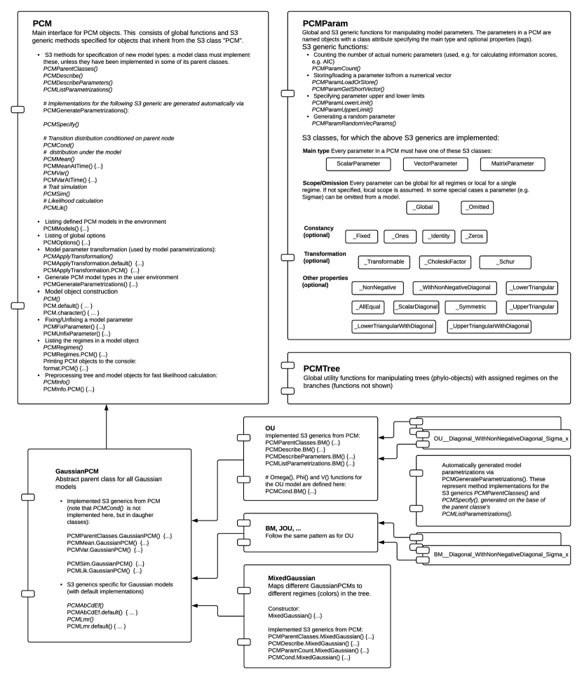
Figure 3: An overview of the PCMBase package. Each box represents a module. The modules “PCM”, “PCMParam” and “PCMTree” define the end-user interface. In particular, the module “PCM” defines the interface for adding model extensions. Function names written in italic style denote S3 generic declarations. These functions can be defined or overwritten by inheriting modules, to provide model-specific behavior. The module “GaussianPCM” implements the pruning-wise likelihood evaluation. The functions $\vec{\omega}$, $\mathbf{\Phi}$ and $\mathbf{V}$ for each model within the framework must be implemented in specifications of the S3 generic function “PCMCond”. It is possible to define parametrizations restricting particular model parameters, e.g. forcing a matrix parameter to be a diagonal matrix.

3.1 Extending PCMBase

Extending the PCMBase functionality can be achieved in two ways:

1. Adding a new model. It is possible to write a new module inheriting from the module “GaussianPCM” and implementing its own version of the functions $\vec{\omega}$, $\mathbf{\Phi}$ and $\mathbf{V}$;

2. Adding a parameterization. It is possible to restrict or apply a transformation to some of the parameters of an already defined model (Fig. 3).

3.2 Using the package

Figure 4 shows the runtime objects and use-cases currently implemented in the PCMBase package.

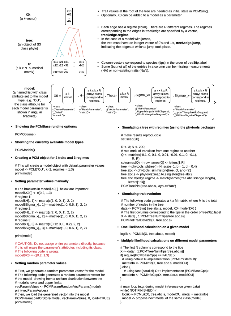
Figure 4: Using the PCMBase package The main runtime objects are depicted on the top of the figure, followed by coding examples for the specific use-cases.

Once the modules for the models of interest have been implemented, the PCMBase package can be used to:

• Creating a model object. The end-user function for creating a model object is PCM(). A model object represents an S3 object, that is, a named list with members corresponding to the model parameters, such as H, Sigma_x and Sigmae_x, and a class attribute equalling the model type, e.g. BM or OU.

• Simulating the evolution of a set of continuous traits along a tree, according to a model. The user level function for trait simulation is PCMSim(). Based on the S3 class of its model argument PCMSim() invokes an appropriate specification of the S3 generic function PCMCond(), which creates a random sampler from the trait distribution at the end of a branch, given the model, the branch length and the trait values at the beginning of the branch.

• Calculating the (log–)likelihood of a model, given a tree and trait values at its tips. The user level function for likelihood calculation is PCMLik(). This function is implemented in the “GaussianPCM” module and inherited by all of its daughter modules. The calculation proceeds in four steps:

  1. Initially, the model-specific functions $\vec{\omega}$, $\mathbf{\Phi}$ and $\mathbf{V}$ are calculated based on the model parameters $\Theta$ and the branch lengths $t_{i}$ (note that this operation does not need the trait values to be present at any tip or internal node in the tree).

  2. Then, the coefficients $\mathbf{A}_{i}$, $\vec{b}_{i}$, $\mathbf{C}_{i}$, $\vec{d}_{i}$, $\mathbf{E}_{i}$ and $f_{i}$ are calculated for each internal and tip node in the tree based on the values $\vec{\omega}$, $\mathbf{\Phi}$ and $\mathbf{V}$ calculated in the previous step. This calculation is done in the function PCMAbCdEf() within the module “GaussianPCM” which, again, is inherited by all model modules (see Fig. 3).

  3. Next, the coefficients $\mathbf{L}_{i}$, $\vec{m}_{i}$, $r_{i}$ are calculated based on the trait values at the tips, the values of $\mathbf{A}_{i}$, $\vec{b}_{i}$, $\mathbf{C}_{i}$, $\vec{d}_{i}$, $\mathbf{E}_{i}$ and $f_{i}$ calculated in the previous step, and the recursive procedure described in Section 2.4, Eqs. (9), (10) and (11).

  4. Finally, the (log–)likelihood value is calculated using the formula

     $$\ell(\Theta)=pdf(\mathbf{X}|\vec{x}_{0},\mathbb{T},\mathbf{\Theta})=\exp\left(\vec{x}_{0}^{T}\mathbf{L}_{0}\vec{x}_{0}+\vec{x}_{0}^{T}\vec{m}_{0}+r_{0}\right),$$ (15)

     where $\Theta$ denotes the set of model parameters and $\vec{x}_{0}$ is treated either as a parameter (specified as a member X0 in the model object) or as the optimum point of the above equation given by:

     $$\vec{x}_{0}=-0.5L_{0}^{-1}\vec{m}_{0}.$$ (16)

The PCMBase-package is licensed under the General Public Licence (GPL) version 3.0. The package and the documentation are accessible from https://github.com/venelin/PCMBase.

3.3 Parallel likelihood calculation with the PCMBaseCpp add–in

For faster likelihood calculation, it is possible to use multiple processor cores to perform the calculation of $\vec{\omega}$, $\mathbf{\Phi}$, $\mathbf{V}$, $\mathbf{A}_{i}$, $\vec{b}_{i}$, $\mathbf{C}_{i}$, $\vec{d}_{i}$, $\mathbf{E}_{i}$ and $f_{i}$ in parallel. This is possible, given the fact that these coefficients depend solely on the model parameters and on the branch lengths in the tree, see, e.g. Eqs. (19) and (20). The calculation of the coefficients $\mathbf{L}_{i}$, $\vec{m}_{i}$, $r_{i}$ is not fully parallelizable but can be divided in parallelizable steps (generations) using a parallel post–order traversal algorithm (Mitov and Stadler, 2017). We implemented this idea in the accompanying package PCMBaseCpp, built on top of the Armadillo template library for linear algebra (Sanderson and Curtin, 2016), the Rcpp package for seamless R and C++ integration (Eddelbuettel, 2013) and the SPLITT library for parallel tree traversal (Mitov and Stadler, 2017).

We compared the performance of the multivariate serial and parallel PCMBase implementation against other univariate and multivariate implementations in a separate work (Mitov and Stadler, 2017). As shown in (Mitov and Stadler, 2017), on contemporary multi-core CPUs, the parallel PCMBaseCpp implementation can speed up the likelihood calculation up to an order of magnitude starting with 2 traits and trees of 100 to 10’000 tips. For univariate OU models, it can be beneficial to implement stand-alone classes bypassing the complex $k\times k$ matrix operations involved in the multivariate case. As shown in (Mitov and Stadler, 2017), this can result in up to $100$ fold faster likelihood calculation in the stand-alone class implementation. The use of PCMBaseCpp as a C++ back-end is recommended even if not using multi-core parallelization, because serial C++ code execution is still nearly $100$ times faster than the equivalent implementation written in R (R–version at time of writing this article was $3.5$).

The PCMBaseCpp-package is licensed under the General Public Licence (GPL) version 3.0. The package is accessible from https://github.com/venelin/PCMBase.

4 Standard extensions

4.1 Missing values

The trait measurement data are the observations at the tips. If a tip is described by a suite of traits it can easily happen that some of them are missing, either due to missing measurement or because the corresponding trait does not exist for the species. Removing such a tip from any further analysis would be wasting information, i.e. the observed data for the tip. We notice that missing measurements for existing traits correspond to the marginal distribution of the observed measurements. In contrast, non-existing traits correspond to reduced dimensionality of the trait vector for the tip in question. Our computational framework keeps track of both of these cases by carefully accounting for the dimensionality of the trait vectors at the tips and the internal nodes and appropriately marginalizing during the integration part, as described below (see also Thm. 4 for examples). The input data is passed as a matrix (rows—trait measurements, columns—different species) the missing measurements have to be indicated as NAs, whereas the non-existing traits have to be indicated as NaNs (fig. 1).

We now turn to describing the technicalities of the mechanism taking care of the missing data. We use a vector of positive integers, $\vec{k}_{j}$, to denote the ordered set of active coordinates for a node $j$. If $j$ is a tip, then $\vec{k}_{j}$ gives the indices of all non–missing entries in the trait vector for $j$; for an internal (unmeasured) node this gives the possibility to make some trait inactive. The cardinality of a vector is denoted with $|\vec{k}|$. For a vector, the notation $\vec{\theta}[\vec{k}]$ means the vector of elements of $\vec{\theta}$ on the coordinates contained in $\vec{k}$, while for a matrix $\mathbf{H}[\vec{k}_{1},\vec{k}_{2}]$ means the matrix $\mathbf{H}$ with only the rows on the coordinates contained in $\vec{k}_{1}$ and columns contained in $\vec{k}_{2}$. For example take $\vec{\theta}=(10,11,12,13)$ and $\vec{k}=(1,3)$, then $\vec{\theta}[\vec{k}]=(10,12)$, while if $\vec{k}_{1}=(1,3)$, $\vec{k}_{2}=(2,4)$ and

$$\mathbf{H}=\left[\begin{array}[]{cccc}10&11&12&13\\ 14&15&16&17\\ 18&19&20&21\\ 22&23&24&25\end{array}\right],$$

then

$$\mathbf{H}[\vec{k}_{1},\vec{k}_{2}]=\left[\begin{array}[]{cccc}11&13\\ 19&21\\ \end{array}\right].$$

If a vector or matrix does not have any indication on which entries it is retained, then it means that we use the whole vector or matrix. All of the above notation is graphically represented in Fig. 1.

In our framework, we have the representation that $\vec{x}_{i}\in\mathbb{R}^{k_{i}}$ conditional on $\vec{x}_{j}\in\mathbb{R}^{k_{j}}$ is $\mathcal{N}(\vec{\omega}_{i}+\mathbf{\Phi}_{i}\vec{x}_{j},\mathbf{V}_{i})$ distributed. By default, PCMBase constructs the coordinate vectors $\vec{k}_{i}$ and $\vec{k}_{j}$ in the following way: for a tip-node, $i$, $\vec{k}_{i}$ contains all observed (neither NA nor NaN) coordinates; for an internal node, $i$ or $j$, the corresponding coordinate vector ($\vec{k}_{i}$ or $\vec{k}_{j}$) contains the coordinates denoting traits that exist (are not NaN) for at least one of the tips descending from that node (Fig. 1). Biologically, this treatment reflects a scenario where all of the traits with at least one non-NaN entry for at least one species (i.e. tip) in the tree must have existed for the root but some of the traits have subsequently disappeared on some lineages of the tree. In particular, if a trait exists for a given tip in the tree, it is assumed that it has existed for all of its ancestors up to the root of the tree. Conversely, if the trait does not exist for a tip, then it has not existed for any of its ancestors up to the first ancestor shared with a tip for which the trait does exist. Different biological scenarios are possible, e.g. assuming that some of the traits did not exist at the root-node but have appeared later for some on the lineages. These can be implemented by accordingly specifying the coordinate vectors.

During likelihood calculation for given trait data, a tree and a trait evolutionary model, the elements $\vec{\omega}_{i}$, $\mathbf{\Phi}_{i}$ and $\mathbf{V}_{i}$ of appropriate dimension are calculated for each non-root node $i$ in the tree. This is done in two steps:

1. The general rule of the model is used to calculate the elements $\tilde{\vec{\omega}}_{i}$, $\tilde{\mathbf{\Phi}}_{i}$, $\tilde{\mathbf{V}}_{i}$ of full dimensionality ($k$), i.e. assuming that all traits exist;

2. Denoting by $j$ the parent node of $i$, the elements $\vec{\omega}_{i}$, $\mathbf{\Phi}_{i}$ and $\mathbf{V}_{i}$ specific for the data in question are obtained as:

   $$\begin{array}[]{rcl}\vec{\omega}_{i}&=&\tilde{\vec{\omega}}_{i}[\vec{k}_{i}],\\ \mathbf{\Phi}_{i}&=&\tilde{\mathbf{\Phi}}_{i}[\vec{k}_{i},\vec{k}_{j}],\\ \mathbf{V}_{i}&=&\tilde{\mathbf{V}}_{i}[\vec{k}_{i},\vec{k}_{i}],\end{array}$$ (17)

   where $\vec{k}_{i}$ and $\vec{k}_{j}$ denote the corresponding coordinate vectors at nodes $i$ and $j$.

4.2 Measurement error

Commonly in PCMs the observed values at the tips are averages from a number of individuals of each species. Using just these average values does not take into account the intra–species variability. Ignoring this can have profound effects on any further estimation (see Hansen and Bartoszek, 2012). Following the PCM tradition, we call this intra–species variability a measurement error, but one should remember that it can be due to true biological variability. Including this variability in our framework is straightforward. One recognizes, which component of the quadratic polynomial representation corresponds to the variance of the tip and augments it by the measurement error variance matrix, see the formulae in Section 5. From the user interface point of view this is a bit more complicated. The measurement error variance matrix is specific to each tip. Therefore in this situation the user has to define for each tip a different regime, with a regime specific variance matrix (called Sigmae_x in the implemented by us classes). Of course other model parameters can also be regime specific, e.g. the deterministic optima (Theta in the implemented by us classes).

4.3 Non–ultrametric trees and multifurcations

If one has only measurements from contemporary species, then the phylogeny describing them is naturally an ultrametric one. However, if for some reason the phylogeny is not ultrametric, e.g. it contains extinct species, then the quadratic polynomial framework can be directly employed. Because each branch is treated separately, it does not matter whether the tree is or is not ultrametric. Therefore, there is no need to search for transformations as in the $3$–point structure based methods. This we believe should make the PCMBase package very straightforward to use. Furthermore, from the proof of Thm. 2 it is obvious that the tree does not need to be binary. Therefore, this adds even more flexibility to the user, they may use trees with polytomies.

4.4 Punctuated equilibrium

It is an ongoing debate in evolutionary biology whether the dominant mode of evolution is a gradual one or whether, during brief periods of time, species undergo rapid change. Any gradual model of evolution can be extended to have a punctuated component by including jumps. Jump mechanisms, like jumps at the start of specific lineages or common jumps for daughter lineages, have to be developed on a per model basis, see Section 5.2 for an example. One current restriction is that PCMBase assumes that lineages do not interact after speciation. It is not possible to implement a model class such that if one daughter lineage jumps the other does not (this is communication between lineages after speciation). Therefore, to have such a situation the user needs to by themselves code on which lineages a jump can take place and on which it cannot. This can be easily achieved using the jumps mechanism of PCMBase. The phylo phylogenetic tree object can be enhanced by a edge.jump binary vector. The length of this vector equals the number of edges in the tree. A $0$ entry indicates that no jump took place on the corresponding branch, while a $1$ entry that it did.

5 Ornstein–Uhlenbeck type models

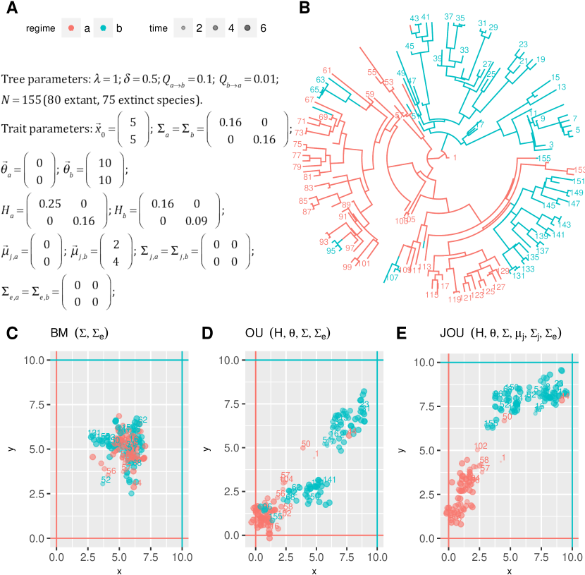
Figure 5: Simulations of trait evolution under four PCMs. A: parameters of the tree simulation ($\lambda$: speciation–rate; $\delta$: extinction–rate; $Q_{a\rightarrow b}$: migration rate from habitat “a” to habitat “b”; $Q_{b\rightarrow a}$: vice–versa of $Q_{a\rightarrow b}$. The other parameters are described in the text. B: A birth–death phylogenetic tree generated using the function pbtree() and sim.history() from the package phytools (Revell, 2011). C—E: scatter plots of the traits observed at the tips of the tree after random simulation using the function PCMSim() of the PCMBase package.

5.1 The phylogenetic Ornstein–Uhlenbeck process

Currently the Ornstein–Uhlenbeck process is the workhorse of the phylogenetic comparative methods framework. Since its introduction by Hansen (1997) it has been considered in detail with multiple software implementations (e.g. Bartoszek et al., 2012; Beaulieu et al., 2012; Butler and King, 2004; Clavel et al., 2015; FitzJohn, 2010; Goolsby et al., 2016; Hansen et al., 2008; Ho and Ané, 2014, to name a few)

In the most general form, the multivariate Ornstein–Uhlenbeck process describes the evolution of a $k$–dimensional suite of traits $\vec{x}\in\mathbb{R}^{k}$ over a period of time by the following stochastic differential equation

$$\mathrm{d}\vec{x}(t)=-\mathbf{H}\left(\vec{x}(t)-\vec{\theta}(t)\right)\mathrm{d}t+\mathbf{\Sigma}_{x}\mathrm{d}\vec{W}(t),$$ (18)

$\mathbf{H}\in\mathbb{R}^{k\times k}$, $\vec{\theta}(t)\in\mathbb{R}^{k}$ and $\mathbf{\Sigma}_{x}\in\mathbb{R}^{k\times k}$. Notice that when $\mathbf{H}=\mathbf{0}$, we obtain a Brownian motion model.

There is no current software package, in the case of phylogenetic OU models, that allows for an arbitrary form of the matrix $\mathbf{H}$. Except for the Brownian motion case, nearly all assume that $\mathbf{H}$ has to be symmetric–positive–definite (note that this encompasses the single trait case). mvMORPH (Clavel et al., 2015), SLOUCH (Hansen et al., 2008) and mvSLOUCH (Bartoszek et al., 2012) seem to be the only exceptions. mvMORPH and mvSLOUCH allow for a general invertible $\mathbf{H}$ (with options to restrict it to diagonal, triangular, symmetric positive–definite, positive eigenvalues, real eigenvalues or generally invertible). Furthermore, mvSLOUCH allows for a special singular structure of $\mathbf{H}$. The matrix has to have in the upper–left–hand corner an invertible matrix (SLOUCH, the univariate predecessor of mvSLOUCH has a scalar here), arbitrary values to the right and $\mathbf{0}$ below. This type of model is called an Ornstein–Uhlenbeck–Brownian motion (OUBM) model. In contrast, when $\mathbf{H}$ is non–singular the model is called an Ornstein–Uhlenbeck–Ornstein–Uhlenbeck (OUOU) one, some variables are labelled as predictors while the rest as responses.

It is of course not satisfactory to have restrictions on the form of $\mathbf{H}$. Different setups have different biological interpretations with regards to modelling causation (see Bartoszek et al., 2012; Reitan et al., 2012). In particular singular matrices will be interesting as they will correspond to certain linear combinations of traits under selection pressures while other linear combinations are free of this. The OUBM model is a special case where a pre–defined group of traits is assumed to evolve marginally as a Brownian motion. Of course a more general setup is desirable and actually, as we show in this work, possible.

Here the the only assumption we make on $\mathbf{H}$ is that it possesses an eigendecomposition, $\mathbf{H}=\mathbf{P}\mathbf{\Lambda}\mathbf{P}^{-1}$ ($\mathbf{\Lambda}$ is a diagonal matrix, and the $i$–th element of the diagonal is denoted as $\lambda_{i}$). In particular $\mathbf{\Lambda}$ can be singular, i.e. some eigenvalues are $0$ and furthermore the eigenvalues/eigenvectors are allowed to be complex.

In this work we assume that $\mathbf{\Sigma}_{x}$ is upper triangular (alternatively lower). Despite how it looks at first sight, this is not any sort of restriction, as in the likelihood we have only $\mathbf{\Sigma}:=\mathbf{\Sigma}_{x}\mathbf{\Sigma}_{x}^{T}$. We furthermore assume that $\mathbf{\Sigma}$ is non–singular, otherwise the whole model would be singular from a statistics point of view.

Most OU model implementations assume that the deterministic optimum $\vec{\theta}_{t}$ is constant along each branch. Different branches may have different levels of it but regime switches along a branch are not allowed (however, Bastide et al., 2018; Ingram and Mahler, 2013; Khabbazian et al., 2016, are exceptions as they attempt to infer points of switching). The PCMBase package does not make any inference but allows for regime switches inside a branch, in the sense that the user (or software using PCMBase’s functionality) has to split the branch into branches having constant regimes.

If we assume that the process starts at a value $\vec{x}(0)=\vec{x}_{0}$, then after evolution over time $t$ (assuming all parameters are constant on this interval) it will be normally distributed with mean vector and variance–covariance matrix (Eqs. (A.1, B.2) Bartoszek et al., 2012)

$$\begin{array}[]{rcl}\operatorname{E}\left[\vec{x}\right](t)&=&e^{-\mathbf{H}t}\vec{x}_{0}+\left(\mathbf{I}-e^{-\mathbf{H}t}\right)\vec{\theta}\in\mathbb{R}^{k}\\ \operatorname{Var}\left[\vec{x}\right](t)&=&\int_{0}^{t}e^{-\mathbf{H}v}\mathbf{\Sigma}e^{-\mathbf{H}^{T}v}\mathrm{d}v\\ &=&\mathbf{P}\left(\left[\frac{1}{\lambda_{i}+\lambda_{j}}\left(1-e^{-(\lambda_{i}+\lambda_{j})t}\right)\right]_{1\leq i,j\leq k}\odot\mathbf{P}^{-1}\mathbf{\Sigma}\mathbf{P}^{-T}\right)\mathbf{P}^{T}\equiv\mathbf{V}(t)\in\mathbb{R}^{k\times k},\end{array}$$ (19)

where $\mathbf{I}$ is the identity matrix of appropriate size. Notice that in the above, $\mathbf{H}$ only enters the moments, through its exponential. Therefore the moments can be calculated (and hence the distribution is well defined) for all $\mathbf{H}$, including defective ones. However, if $\mathbf{H}$ has (as we assumed) an eigendecomposition, then the exponential and in turn variance formula can be calculated effectively. If $\lambda_{i}=\lambda_{j}=0$, then the term in the variance has to be treated in the limiting sense $\lambda^{-1}(1-e^{-\lambda t})\to t$ with $\lambda\to 0$. Therefore, the variance matrix is always well defined and never singular for $t>0$.

We assumed that $\mathbf{H}$ has to have an eigendecomposition while the process is well defined for any $\mathbf{H}$, including defective ones. Calculation of the matrix exponential for a defective matrix can be done using Jordan block decomposition. However, we do not provide such functionality, as Jordan block decomposition is numerically unstable and in fact, we are not aware of any R implementation of it. Hence, defective matrices will result in errors. However, it is important to remember that defectiveness is the exception and not the rule for matrices. If checked for (by e.g. checking if the eigenvector matrix from eigen()’s output is non–singular, Corollary $7$.$1$.$8$., p. $353$ Golub and Van Loan, 2013) and handled before calling using our package, it should not cause major issues.

We now turn to showing how to construct the composite parameters found in the proof of Thm. 1 from the OU process representation of Eq. (18).

To simplify notation we denote the defined in Eq. (19) covariance matrix as $\tilde{\mathbf{V}}_{i}\equiv\mathbf{V}(t_{i})+\delta_{i\in\{\mathbb{T}_{0}^{\prime}s\leavevmode\nobreak\ tips\}}\mathbf{\Sigma}_{e}^{i}$, where the Kronecker $\delta$–symbol is defined as $\delta_{i\in\{\mathbb{T}_{0}^{\prime}s\leavevmode\nobreak\ tips\}}=1$ if $i$ is a tip of the tree and $\delta_{i\in\{\mathbb{T}_{0}^{\prime}s\leavevmode\nobreak\ tips\}}=0$. The matrix $\mathbf{\Sigma}_{e}^{i}$ is the measurement error or intra–species variability variance matrix for tip species $i$.

Theorem 4.

Let $\vec{k}_{i}$ be the vector of coordinates on which $\vec{x}_{i}$ is observed, $\vec{k}_{j}$ be the vector of coordinates for $\vec{x}_{j}$ and $\vec{k}$ the full vector of coordinates. Using the parameterization found in the proof of Thm. 1 a multivariate Ornstein–Uhlenbeck process of evolution can be represented as

$$\begin{array}[]{rcl}\mathbf{V}_{i}&=&\tilde{\mathbf{V}}_{i}[\vec{k}_{i},\vec{k}_{i}]\in\mathbb{R}^{|\vec{k}_{i}|\times|\vec{k}_{i}|},\\ \vec{\omega}_{i}&=&\left(\mathbf{I}[\vec{k}_{i},\vec{k}]-e^{-\mathbf{H}t_{i}}[\vec{k}_{i},\vec{k}]\right)\vec{\theta}_{i}[\vec{k}]\in\mathbb{R}^{|\vec{k}_{i}|},\\ \mathbf{\Phi}_{i}&=&e^{-\mathbf{H}t_{i}}[\vec{k}_{i},\vec{k}_{j}]\in\mathbb{R}^{|\vec{k}_{i}|\times|\vec{k}_{j}|}.\end{array}$$ (20)

Proof.

In the multivariate OU case, Eq. (2) will be

$$pdf(\vec{x}_{i}|\vec{x}_{j},t_{i})=\mathcal{N}\left(e^{-\mathbf{H}t_{i}}[\vec{k}_{i},\vec{k}_{j}]\vec{x}_{j}+\left(\mathbf{I}[\vec{k}_{i},\vec{k}]-e^{-\mathbf{H}t_{i}}[\vec{k}_{i},\vec{k}]\right)\vec{\theta}_{i}[\vec{k}],\mathbf{V}_{i}[\vec{k}_{i},\vec{k}_{i}]\right).$$

∎

These formulae do not depend on whether the eigenvalues of $\mathbf{H}$ are positive, negative or $0$. They will still be correct. The exponentiation of $\mathbf{H}$ will also not depend on this. Only with $\mathbf{V}_{i}$ will we need to take an appropriate limit as an eigenvalue is $0$, see comments after Eq. (19).

Corollary 1.

For a multivariate Brownian motion process of evolution, we have $\mathbf{H}=\mathbf{0}$ and $\tilde{\mathbf{V}}_{i}=t_{i}\mathbf{\Sigma}+\delta_{i\in\{\mathbb{T}_{0}^{\prime}s\leavevmode\nobreak\ tips\}}\mathbf{\Sigma}_{e}^{i}$. Hence, using the parametrization found in the proof of Thm. 1 one can represent it as

$$\begin{array}[]{rcl}\mathbf{V}_{i}&=&\tilde{\mathbf{V}}_{i}[\vec{k}_{i},\vec{k}_{i}]\in\mathbb{R}^{|\vec{k}_{i}|\times|\vec{k}_{i}|},\\ \vec{\omega}_{i}&=&\vec{0}[\vec{k}_{i}]\in\mathbb{R}^{|\vec{k}_{i}|},\\ \mathbf{\Phi}_{i}&=&\mathbf{I}[\vec{k}_{i},\vec{k}_{j}]\in\mathbb{R}^{|\vec{k}_{i}|\times|\vec{k}_{j}|}.\end{array}$$ (21)

In Fig. 5, panel C, one can see an example collection of tip observations resulting from simulating of a bivariate trait following a BM process on top of a phylogeny and in panel D following an OU process.

5.2 Multivariate Ornstein–Uhlenbeck with jumps

It is an ongoing debate in evolutionary biology at what time does evolutionary change take place. Change may take place either at times of speciation (punctuated equilibrium Eldredge and Gould, 1972; Gould and Eldredge, 1993) or gradually accumulate (phyletic gradualism, see references in Eldredge and Gould, 1972). There seems to be evidence for both types of evolution. For example, Bokma (2002) discusses that punctuated equilibrium is supported by fossil records (see Eldredge and Gould, 1972) but on the other hand Stebbins and Ayala (1981) also indicate experiments supporting phyletic gradualism.

At an internal node in the tree something happens that drives species apart and then “The further removed in time a species from the original speciation event that originated it, the more its genotype will have become stabilized and the more it is likely to resist change.” (Mayr, 1982). Between branching events (and jumps) we can have stasis—“fluctuations of little or no accumulated consequence” taking place (Gould and Eldredge, 1993). Therefore, one would want processes that incorporate both types of evolution and allow for testing if either of them dominates. Ornstein–Uhlenbeck with jumps models are a framework where this is possible. Shortly, along a branch the traits follows an OU process. But then, just after speciation, a jump in the traits’ values can take place. Whether such a jump takes place on a given, some or all daughter lineages is up to the specific implementation of the framework. From the perspective of the PCMBase package the location of the jumps has to be provided. It is in fact also possible in our implementation, to place jumps at arbitrary points inside a branch (this may be necessary if speciation events are missing due to unsampled extinct or extant species). Inferring of where jumps took place are at a different level of PCM modelling, then what PCMBase handles.

Ornstein–Uhlenbeck processes with jumps capture the key idea behind the theory of punctuated equilibrium. If the speed of convergence of the process is large enough, then the stationary distribution is approached rapidly and the stationary oscillations around the (constant) mean can be interpreted as stasis between jumps.

Corollary 2.

For a multivariate OU defined with jumps, jump distribution $\mathcal{N}(\vec{\mu}_{J},\mathbf{\Sigma}_{J})$ and denoting by the indicator $\xi_{i}$ (we assume that the jumps are known) if a jump took place at the start of the branch leading to node $i$, we have

$$\begin{array}[]{rcl}\tilde{\mathbf{V}}_{i}&=&\int\limits_{0}^{t_{i}}e^{-\mathbf{H}v}\mathbf{\Sigma}e^{-\mathbf{H}^{T}v}\mathrm{d}v+\xi_{i}e^{-\mathbf{H}t_{i}}\mathbf{\Sigma}_{J}e^{-\mathbf{H}^{T}t_{i}}+\delta_{i\in\{\mathbb{T}_{0}^{\prime}s\leavevmode\nobreak\ tips\}}\mathbf{\Sigma}_{e}^{i}.\end{array}$$ (22)

Using the parametrization found in the proof of Thm. 1 one can represent it as

$$\begin{array}[]{rcl}\mathbf{V}_{i}&=&\tilde{\mathbf{V}}_{i}[\vec{k}_{i},\vec{k}_{i}]\in\mathbb{R}^{|\vec{k}_{i}|\times|\vec{k}_{i}|},\\ \vec{\omega}_{i}&=&\xi_{i}e^{-\mathbf{H}t_{i}}[\vec{k}_{i},\vec{k}]\vec{\mu}_{J}[\vec{k}]+\left(\mathbf{I}[\vec{k}_{i},\vec{k}]-e^{-\mathbf{H}t_{i}}[\vec{k}_{i},\vec{k}]\right)\vec{\theta}_{i}[\vec{k}]\in\mathbb{R}^{|\vec{k}_{i}|},\\ \mathbf{\Phi}_{i}&=&e^{-\mathbf{H}t_{i}}[\vec{k}_{i},\vec{k}_{j}]\in\mathbb{R}^{|\vec{k}_{i}|\times|\vec{k}_{j}|}.\end{array}$$ (23)

The multivariate Brownian motion with jumps model follows as an immediate corollary $(\mathbf{H}\to\mathbf{0})$ .

Corollary 3.

For a multivariate Brownian motion with jumps (jumps defined the same as in Corollary 2) the variance at a node $i$ is $\tilde{\mathbf{V}}_{i}=t_{i}\mathbf{\Sigma}[\vec{k}_{i},\vec{k}_{i}]+\xi_{i}\mathbf{\Sigma}_{J}[\vec{k}_{i},\vec{k}_{i}]+\delta_{i\in\{\mathbb{T}_{0}^{\prime}s\leavevmode\nobreak\ tips\}}\mathbf{\Sigma}_{e}^{i}$. Using the parametrization found in the proof of Thm. 1 one can represent it as

$$\begin{array}[]{rcl}\mathbf{V}_{i}&=&\tilde{\mathbf{V}}_{i}[\vec{k}_{i},\vec{k}_{i}]\in\mathbb{R}^{|\vec{k}_{i}|\times|\vec{k}_{i}|},\\ \vec{\omega}_{i}&=&\xi_{i}\vec{\mu}_{J}[\vec{k}_{i}]\in\mathbb{R}^{|\vec{k}_{i}|},\\ \mathbf{\Phi}_{i}&=&\mathbf{I}[\vec{k}_{i},\vec{k}_{j}]\in\mathbb{R}^{|\vec{k}_{i}|\times|\vec{k}_{j}|}.\end{array}$$ (24)

In Fig. 5, panel E, one can see an example collection of tip observations resulting from simulating of a bivariate trait following an OU process with jumps on top of a phylogeny.

5.3 Beyond the Ornstein–Uhlenbeck process

There are a number of popular PCM models that do not fall into the above described OU framework despite appearing very similar. In particular we mean the BM with trend, drift, early burst/Accelerating–decelerating (EB/ACDC) or white noise (implemented in the geiger R package Harmon et al., 2008). With the exception of white noise, they all can be represented by the SDE (cf. Eq. (1) of Manceau et al., 2016)

$$\left\{\begin{array}[]{rcl}\mathrm{d}\vec{x}(t)&=&\left(\vec{h}(t)-\mathbf{H}\vec{x}(t)\right)\mathrm{d}t+\mathbf{\Gamma}(t)\mathrm{d}\vec{W}(t),\\ \vec{x}(0)&=&\vec{x}_{0}.\end{array}\right.$$ (25)

Notice that setting $\vec{h}(t)=\vec{\theta}$ and $\mathbf{\Gamma}(t)=\mathbf{\Sigma}_{x}$ to constants we recover the “usual” OU process, considered in Thm. 4. Manceau et al. (2016) provide the expectation and variance under the model, by slightly modifying their Eqs. (4a) and (4b),

$$\begin{array}[]{rcl}\operatorname{E}\left[\vec{x}_{i}|\vec{x}_{j}\right]&=&e^{-t_{i}\mathbf{H}_{i}}\vec{x}_{j}+\int\limits_{t_{i}^{s}}^{t_{i}^{e}}e^{(s-t_{i}^{e})\mathbf{H}_{i}}\vec{h}_{i}(s)\mathrm{d}s,\\ \operatorname{Var}\left[\vec{x}_{i}|\vec{x}_{j}\right]&=&\int\limits_{t_{i}^{s}}^{t_{i}^{e}}e^{(s-t_{i}^{e})\mathbf{H}_{i}}\mathbf{\Gamma}_{i}(s)\mathbf{\Gamma}_{i}^{T}(s)e^{(s-t_{i}^{e})\mathbf{H}_{i}^{T}}\mathrm{d}s,\end{array}$$ (26)

where $t_{i}^{s}$ is the time at the start of the branch and $t_{i}^{e}$ at the end (of course $t_{i}=t_{i}^{e}-t_{i}^{s}$). This corresponds in our framework to

$$\begin{array}[]{rcl}\vec{\omega}_{i}&=&\int\limits_{t_{i}^{s}}^{t_{i}^{e}}e^{(s-t_{i}^{e})\mathbf{H}_{i}}\vec{h}_{i}(s)\mathrm{d}s,\\ \mathbf{\Phi}_{i}&=&e^{-t_{i}\mathbf{H}_{i}},\\ \mathbf{V}_{i}&=&\int\limits_{t_{i}^{s}}^{t_{i}^{e}}e^{(s-t_{i}^{e})\mathbf{H}_{i}}\mathbf{\Gamma}_{i}(s)\mathbf{\Gamma}_{i}^{T}(s)e^{(s-t_{i}^{e})\mathbf{H}_{i}^{T}}\mathrm{d}s.\end{array}$$ (27)

Hence, in the subcase of non–interacting lineages, our framework covers Manceau et al. (2016)’s. As the initially mentioned models are subcases (cf. Tab. 1 of Manceau et al., 2016) they are available in our framework. To obtain the values of the $\vec{\omega}_{i}$, $\mathbf{\Phi}_{i}$ and $\mathbf{V}_{i}$ parameters in Eq. (27) one has to either analytically calculate the integrals for specific $\vec{h}_{i}(\cdot)$ and $\mathbf{\Gamma}(\cdot)$ functions or consider a general numerical integration scheme.

Apart from the previously considered OU model, for some other typical PCM models the integrals can be evaluated analytically.

1. ACDC model (after generalizing the one dimensional model presented by Blomberg et al., 2003; Harmon et al., 2010, to the multivariate case)

   $$\begin{array}[]{rcl}\vec{\omega}_{i}&=&\vec{0},\\ \mathbf{\Phi}_{i}&=&\mathbf{I},\\ \mathbf{V}_{i}&=&\int_{t_{i}^{s}}^{t_{i}^{e}}e^{s\mathbf{R}_{i}}\mathbf{\Sigma}_{i}\mathbf{\Sigma}_{i}^{T}e^{s\mathbf{R}_{i}^{T}}\mathrm{d}s.\end{array}$$ (28)

   See Eq. (19) for how to calculate the integral, for $\mathbf{V}_{i}$, when the matrix $\mathbf{R}$ is eigendecomposable.

2. BM with drift

   $$\begin{array}[]{rcl}\vec{\omega}_{i}&=&\vec{h}_{i}t_{i},\\ \mathbf{\Phi}_{i}&=&\mathbf{I},\\ \mathbf{V}_{i}&=&\mathbf{\Sigma}_{i}\mathbf{\Sigma}_{i}^{T}t_{i}.\end{array}$$ (29)

3. BM with trend—in the most general setup of a linear form under the integral for $\mathbf{V}_{i}$ (based on the Supporting Information of Harmon et al., 2010, in the one dimensional case)

   $$\begin{array}[]{rcl}\vec{\omega}_{i}&=&\vec{0},\\ \mathbf{\Phi}_{i}&=&\mathbf{I},\\ \mathbf{V}_{i}&=&\int^{t_{i}^{s}+t_{i}}_{t_{i}^{s}}\left(\mathbf{U}s+\mathbf{W}\right)\mathrm{d}s=\mathbf{U}\frac{t_{i}^{2}}{2}+\mathbf{W}t_{i}.\end{array}$$ (30)

4. The white noise process corresponds to a situation, where the phylogeny does not contribute to the covariance structure between the species, so that the all species are regarded as independent identically distributed observations of the same multivariate Gaussian distribution with global mean $\vec{x}_{0}=\vec{\mu}$ and same variance–covariance matrix $\mathbf{\Sigma_{e}}$.

Naturally everything should be appropriately (as described in Section 4.1) adjusted if missing values are present.

6 Technical correctness

Validating the technical correctness is an important but often neglected step in the development of likelihood calculation software. This step is particularly relevant for complex multivariate models, because logical errors can occur in many levels, such as the mathematical equations for the different terms involved in the likelihood, the programming code implementing these equations, the code responsible for the tree traversal, the parametrization of the model and the preprocessing of the input data. These logical errors add up to numerical errors caused by limited floating point precision, which can be extremely hard to identify. Ultimately, these errors lead to wrong likelihood values, false parameter inference and wrong analysis. All these concerns motivate for a systematic approach of testing the correctness of the software.

We implemented a technical correctness test of the three models currently implemented in PCMBase using the method of posterior quantiles proposed by Cook et al. (2006). The posterior quantiles method (Alg. 1) is a simulation based approach. It employs the fact that, for a fixed prior distribution of the model parameters, the sample of posterior quantiles of any model parameter, $\theta$ is uniform (see e.g. Cook et al., 2006; Mitov and Stadler, 2017, for details). Thus, any deviation from uniformity of the posterior quantile sample for any of the model parameters indicates the presence of an error, either in the simulation software, or in the likelihood calculator used to generate the posterior samples.

Algorithm 1 Posterior quantiles method

1:Sample “true” parameters $\Theta$ from the prior;

2:Simulate random data, $\mathbf{X}_{\Theta}$, under the model specified by $\Theta$;

3:Generate a sample $S_{\theta}$ from the posterior distribution $P_{\theta}=P(\theta|\mathbf{X}_{\Theta})$;

4:Calculate the empirical quantile of the “true” $\theta$ in $S_{\theta}$;

We used a fixed non–ultrametric tree of $N=515$ tips with two regimes “a” and “b”. The tree was generated using the functions pbtree() and sim.history() from the package phytools (Revell, 2011). We implemented the posterior quantile test using the BayesValidate R–package (Cook et al., 2006). For each model we set a parametrization and a prior distribution as follows:

• BM 3 parameters: $\Theta_{BM}=[\Sigma_{11},\Sigma_{12},\Sigma_{e,11}]$, such that

  $${\mathbf{\Sigma}_{a}}=\left({\begin{array}[]{*{20}{c}}{\Sigma_{11}}&{\Sigma_{12}}\\ {\Sigma_{12}}&{\Sigma_{11}}\end{array}}\right),\,{\mathbf{\Sigma}_{b}}=\left({\begin{array}[]{*{20}{c}}{\Sigma_{11}}&{0}\\ {0}&{\Sigma_{11}}\end{array}}\right),\,{\mathbf{\Sigma}_{e,a}}={\mathbf{\Sigma}_{e,b}}=\left({\begin{array}[]{*{20}{c}}{\Sigma_{e,11}}&{0}\\ {0}&{\Sigma_{e,11}}\end{array}}\right)$$

  prior: $\Sigma_{11}\sim\text{Exp}(1),\,\Sigma_{12}\sim\mathcal{U}(-0.9\Sigma_{11},\,0.9\Sigma_{11}),\,\Sigma_{e,11}\sim\text{Exp}(10)$.

• OU 8 parameters: $\Theta_{OU}=[\Theta_{BM},\theta_{b,1},\theta_{b,2},H_{b,11},H_{b,12},H_{b,22}]$, such that $\mathbf{\Sigma}_{a}$, $\mathbf{\Sigma}_{b}$, $\mathbf{\Sigma}_{e,a}$ and $\mathbf{\Sigma}_{e,b}$ are defined as for BM and

  $${\vec{\theta}_{a}}=\left({\begin{array}[]{*{20}{c}}{0}\\ {0}\end{array}}\right),\,{\vec{\theta}_{b}}=\left({\begin{array}[]{*{20}{c}}{\theta_{b,1}}\\ {\theta_{b,2}}\end{array}}\right),\,{\mathbf{H}_{a}}=\left({\begin{array}[]{*{20}{c}}{0}&{0}\\ {0}&{0}\end{array}}\right),\,{\mathbf{H}_{b}}=\left({\begin{array}[]{*{20}{c}}{H_{b,11}}&{H_{b,12}}\\ {H_{b,12}}&{H_{b,11}}\end{array}}\right)$$

  prior: for parameters in $\Theta_{BM}$ the same prior has been used as for the BM model; for the new parameters, the prior has been set as $\theta_{b,1}\sim\mathcal{N}(1,.25),\,\theta_{b,2}\sim\mathcal{N}(2,.5),\,H_{b,11}\sim\text{Exp}(1),\,H_{b,22}\sim\text{Exp}(1),\,H_{b,12}\sim\mathcal{U}(-0.9\sqrt{H_{b,11}H_{b,22}},\,0.9\sqrt{H_{b,11}H_{b,22}})$.

• JOU 9 parameters: $\Theta_{JOU}=[\Theta_{OU},\Sigma_{j,11}]$, such that $\mathbf{\Sigma}_{a}$, $\mathbf{\Sigma}_{b}$, $\mathbf{\Sigma}_{e,a}$, $\mathbf{\Sigma}_{e,b}$, $\vec{\theta}_{a}$, $\vec{\theta}_{b}$, $\mathbf{H}_{a}$, $\mathbf{H}_{b}$ are defined as for OU and

  $${\vec{\mu}_{j,a}}=\left({\begin{array}[]{*{20}{c}}{-\theta_{b,1}}\\ {-\theta_{b,2}}\end{array}}\right),\,{\vec{\mu}_{j,b}}=\left({\begin{array}[]{*{20}{c}}{\theta_{b,1}}\\ {\theta_{b,2}}\end{array}}\right),\,{\mathbf{\Sigma}_{j,a}}=\left({\begin{array}[]{*{20}{c}}{1}&{0}\\ {0}&{1}\end{array}}\right),\,{\mathbf{\Sigma}_{j,b}}=\left({\begin{array}[]{*{20}{c}}{\Sigma_{j,11}}&{0}\\ {0}&{\Sigma_{j,11}}\end{array}}\right)$$

  prior: for parameters in $\Theta_{OU}$ the same prior has been used as for the OU model; for the new parameter, the prior has been set as $\Sigma_{j,11}\sim\text{Exp}(10)$.

For each, model, we ran the function validate() from the BayesValidate package, setting the number of replications to $48$. The results are summarized in Fig. 6. All Bonferroni adjusted p–values of the absolute $Z_{\theta}$ statistics were above $0.2$, showing that the posterior quantiles did not deviate from uniformity (see Cook et al., 2006, for details on $Z_{\theta}$ statistic).

Figure 6: Absolute $Z_{\theta}$–statistics for the four posterior quantile tests. The $Z_{\theta}$ statistic is described by Cook et al. (2006). High values indicate deviation from uniformity of the posterior quantile distribution for an individual model parameter (circles) or a batch of several model parameters (bullets). The reported values, smaller than 3 for all parameters, had insignificant p-values as well as Bonferroni–adjusted p–values. The plots were generated using the package BayesValidate (Cook et al., 2006).

7 Discussion

Currently the mathematical frameworks proposed for PCMs are applied to situations that are very different from the original motivation of a between species analyses within a small clade of some quantitative trait. They are employed in many situations with a tree structure behind the measurements. For example, traits being gene expression levels (Bedford and Hartl, 2009; Rohlfs et al., 2013) or epidemiological measurements (the tree connects the epidemic’s outbursts Pybus et al., 2012) are analysed. With large and diverse clades, there is a need to vary the parameters of the models across different clades or epochs in the tree. Already e.g. Bartoszek et al. (2012); Butler and King (2004); Hansen (1997) showed the possibility of varying the deterministic optimum of OU processes. Beaulieu et al. (2012); Eastman et al. (2011); Manceau et al. (2016) went further to allow all parameters of the underlying SDE to vary over the tree. Estimating the time and branches for parameter changes has been proposed in Eastman et al. (2011), Ingram and Mahler (2013), Khabbazian et al. (2016) and Bastide et al. (2018) with implementations in AUTEUR, SURFACE, $l$1ou and PhylogeneticEM R respectively.

The situations mentioned above can easily require likelihood evaluations well beyond the amount of a “standard” optimization (e.g. an exponential number of regime patterns on the tree or reestimation to obtain the estimators’ distribution). Furthermore, the trees connected to such calculations to be analysed can be huge, going into thousands of tips such as HIV data analysed e.g. in (Hodcroft et al., 2014; Mitov and Stadler, 2018). Hence, being able to quickly evaluate the likelihood is crucial. The PCMBase package offers this possibility for fast likelihood calculation for all models in the $\mathcal{G}_{LInv}$-family, including mixed–type models, where different types of models are realized on different parts of the phylogenetic tree. Further, it is extremely flexible allowing the user to easily use it as a computational engine for their particular modelling setup/parametrization. PCMBase is able to handle multiple standard extensions, allowing the scientist to use all observed data. Finally, the package is written in such a way that it can be further developed to include more complex situations.

Some “standard extensions” from Section 4 deserve special mention. Firstly and briefly we remind the reader that PCMBase handles non–ultrametric (Section 4.3) trees. Thus it can directly use fossil data or pathogen data. In the same Section 4.3, we notice that from the perspective of PCMBase the out–degree of an internal node is irrelevant. This is as the likelihood is calculated as the product over all daughter clades. Therefore, our computational engine should be appreciated by users who have poorly resolved trees with polytomies.

PCMBase handles incomplete observations of traits, meaning partially measured fossils do not pose any problem. As mentioned in Section 4.1 PCMBase distinguishes two types of missingness, unobserved trait (NA) and non–existing trait (NaN). From the perspective of the user this might seem like a mere formality. However, from the perspective of the likelihood calculations it makes a profound difference. Unobserved traits are integrated over, meaning that first $\vec{\omega}_{i}$, $\mathbf{V}_{i}$, $\mathbf{\Phi}_{i}$ are calculated as if all $k$ traits were present and only afterwards are appropriate entries/rows and columns removed. The second case of non–existing traits is treated differently, $\vec{\omega}_{i}$, $\mathbf{V}_{i}$, $\mathbf{\Phi}_{i}$ are calculated taking into account that the trait vector at the given node is from a lower dimension (i.e. $\mathbf{A}_{i}$, $\vec{b}_{i}$, $\mathbf{C}_{i}$, $\vec{d}_{i}$ and $\mathbf{E}_{i}$ are taken from lower dimensions by removing appropriate entries/rows and columns).

Despite the generality, speed and easiness of use of the package the user has to be aware of a potential pitfall. Theorem 1 and the proof of Thm. 2 indicate a numerical weakness of our method. If a branch ending at node $i$ is extremely short, then the associated with it variance–covariance matrix, $\mathbf{V}_{i}$, can be computationally singular. Hence, calculating its inverse, a necessary step to obtain the likelihood, will not be possible. PCMBase catches such an error and returns it, pointing to the offending node. As an alternative, it is possible to tolerate such an error: if the branch is shorter than a user-specified threshold (runtime options PCMBase.Skip.Singular and PCMBase.Threshold.Skip.Singular), the whole branch can be treated as a $0$–length branch and skipped during the likelihood calculation.

All models above assume that the trait evolves on the tree structure, i.e. does not influence the branching pattern. However, there are tools such as diversitree which assume that the trait determines branching rates. Those approaches assume a single model and parameters across the whole tree though and it will be a future challenge to generalize them towards multiple regimes on a single tree, as we did here for the $\mathcal{G}_{LInv}$-models.

References

- Bartoszek (2014) Bartoszek, K., 2014. Quantifying the effects of anagenetic and cladogenetic evolution. Mathematical Biosciences 254, 42–57.
- Bartoszek et al. (2012) Bartoszek, K., Pienaar, J., Mostad, P., Andersson, S., Hansen, T.F., 2012. A phylogenetic comparative method for studying multivariate adaptation. Journal of Theoretical Biology 314, 204–215.
- Bastide et al. (2018) Bastide, P., Ané, C., Robin, S., Mariadassou, M., 2018. Inference of adaptive shifts for multivariate correlated traits. Systematic Biology 113, 2158–680.
- Beaulieu et al. (2012) Beaulieu, J.M., Jhwueng, D.C., Boettiger, C., O’Meara, B.C., 2012. Modeling stabilizing selection: expanding the Ornstein–Uhlenbeck model Of adaptive evolution. Evolution 66, 2369–2383.
- Bedford and Hartl (2009) Bedford, T., Hartl, D.L., 2009. Optimization of gene expression by natural selection, in: Proceedings of the National Academy of Sciences, Department of Organismic and Evolutionary Biology, Harvard University, 16 Divinity Avenue, Cambridge, MA 02138. National Academy of Sciences. pp. 1133–1138.
- Blomberg (2017) Blomberg, S.P., 2017. Beyond Brownian motion and the Ornstein-Uhlenbeck process: Stochastic diffusion models for the evolution of quantitative characters. bioRxiv , 067363.
- Blomberg et al. (2003) Blomberg, S.P., Garland, T.J., Ives, A.R., 2003. Testing for phylogenetic signal in comparative data: behavioral traits are more labile. Evolution 57, 717–745.
- Bokma (2002) Bokma, F., 2002. Detection of punctuated equilibrium from molecular phylogenies. Journal of Evolutionary Biology 15, 1048–1056.
- Boucher et al. (2018) Boucher, F.C., Démery, V., Conti, E., Harmon, L.J., Uyeda, J., 2018. A general model for estimating macroevolutionary landscapes. Systematic Biology 67, 304–319.
- Butler and King (2004) Butler, M.A., King, A.A., 2004. Phylogenetic comparative analysis: A modeling approach for adaptive evolution. American Naturalist 164, 683–695.
- Clavel et al. (2015) Clavel, J., Escarguel, G., Merceron, G., 2015. mvmorph: an R package for fitting multivariate evolutionary models to morphometric data. Methods in Ecology and Evolution 6, 1311–1319.
- Cook et al. (2006) Cook, S.R., Gelman, A., Rubin, D.B., 2006. Validation of software for Bayesian models using posterior quantiles. Journal of Computational and Graphical Statistics 15, 675–692.
- Duchen et al. (2017) Duchen, P., Leuenberger, C., Szilágyi, S.M., Harmon, L., Eastman, J., Schweizer, M., Wegmann, D., 2017. Inference of evolutionary jumps in large phylogenies using Lévy processes. Systematic Biology 66, 950–963.
- Eastman et al. (2011) Eastman, J.M., Alfaro, M.E., Joyce, P., Hipp, A.L., Harmon, L.J., 2011. A novel comparative method for identifying shifts in the rate of character evolution on trees. Evolution 65, 3578–3589.
- Eddelbuettel (2013) Eddelbuettel, D., 2013. Seamless R and C++ Integration with Rcpp. Springer Science & Business Media, New York, NY.
- Edwards (1970) Edwards, A.W.F., 1970. Estimation of the branch points of a branching diffusion process (With discussion). Journal of the Royal Statistical Society. Series B. Methodological 32, 155–174.
- Eldredge and Gould (1972) Eldredge, N., Gould, S.J., 1972. Punctuated equilibria: an alternative to phyletic gradualism, in: Schopf, T.J.M., Thomas, J.M. (Eds.), Models in Paleobiology. Freeman Cooper, San Francisco, pp. 82–115.
- Felsenstein (1973) Felsenstein, J., 1973. Maximum–likelihood estimation of evolutionary trees from continuous characters. American Journal of Human Genetics 25, 471–492.
- Felsenstein (1985) Felsenstein, J., 1985. Phylogenies and the comparative method. The American Naturalist 125, 1–15.
- Felsenstein (1988) Felsenstein, J., 1988. Phylogenies and quantitative characters. Annual Review of Ecology and Systematics 19, 445–471.
- FitzJohn (2010) FitzJohn, R.G., 2010. Quantitative traits and diversification. Systematic Biology 59, 619–633.
- FitzJohn (2012) FitzJohn, R.G., 2012. Diversitree: comparative phylogenetic analyses of diversification in R. Methods in Ecology and Evolution 3, 1084–1092.
- Freckleton (2012) Freckleton, R.P., 2012. Fast likelihood calculations for comparative analyses. Methods in Ecology and Evolution 3, 940–947.
- Golub and Van Loan (2013) Golub, G.H., Van Loan, C.F., 2013. Matrix Computations. The Johns Hopkins University Press, Baltimore.
- Goolsby et al. (2016) Goolsby, E.W., Bruggeman, J., Ané, C., 2016. Rphylopars: fast multivariate phylogenetic comparative methods for missing data and within–species variation. Methods in Ecology and Evolution 8, 22–27.
- Gould and Eldredge (1993) Gould, S.J., Eldredge, N., 1993. Punctuated equilibrium comes of age. Nature 366, 223–227.
- Hansen (1997) Hansen, T.F., 1997. Stabilizing selection and the comparative analysis of adaptation. Evolution 51, 1341–1351.
- Hansen and Bartoszek (2012) Hansen, T.F., Bartoszek, K., 2012. Interpreting the evolutionary regression: the interplay between observational and biological errors in phylogenetic comparative studies. Systematic Biology 61, 413–425.
- Hansen et al. (2008) Hansen, T.F., Pienaar, J., Orzack, S.H., 2008. A comparative method for studying adaptation to a randomly evolving environment. Evolution 62, 1965–1977.
- Harmon et al. (2010) Harmon, L.J., Losos, J.B., Jonathan Davies, T., Gillespie, R.G., Gittleman, J.L., Bryan Jennings, W., Kozak, K.H., McPeek, M.A., Moreno-Roark, F., Near, T.J., Purvis, A., Ricklefs, R.E., Schluter, D., Schulte II, J.A., Seehausen, O., Sidlauskas, B.L., Torres-Carvajal, O., Weir, J.T., Mooers, A.Ø., 2010. Early bursts of body size and shape evolution are rare in comparative data. Evolution 64, 2385–2396.
- Harmon et al. (2008) Harmon, L.J., Weir, J.T., Brock, C.D., Glor, R.E., Challenger, W., 2008. GEIGER: investigating evolutionary radiations. Bioinformatics 24, 129–131.
- Ho and Ané (2014) Ho, L.s.T., Ané, C., 2014. A linear–time algorithm for Gaussian and non-Gaussian trait evolution models. Systematic Biology 63, 397–408.
- Hodcroft et al. (2014) Hodcroft, E., Hadfield, J.D., Fearnhill, E., Phillips, A., Dunn, D., O’Shea, S., Pillay, D., Brown, A.J.L., 2014. The contribution of viral genotype to plasma viral set–point in HIV infection. PLoS Pathogens 10, e1004112.
- Ingram and Mahler (2013) Ingram, T., Mahler, D.L., 2013. SURFACE: detecting convergent evolution from comparative data by fitting Ornstein–Uhlenbeck models with stepwise Akaike Information Criterion. Methods in Ecology and Evolution 4, 416–425.
- Khabbazian et al. (2016) Khabbazian, M., Kriebel, R., Rohe, K., Ané, C., 2016. Fast and accurate detection of evolutionary shifts in Ornstein–Uhlenbeck models. Methods in Ecology and Evolution 7, 811–824.
- Lande (1976) Lande, R., 1976. Natural–selection and random genetic drift in phenotypic evolution. Evolution 30, 314–334.
- Landis et al. (2012) Landis, M.J., Schraiber, J.G., Liang, M., 2012. Phylogenetic analysis using Lévy processes: finding jumps in the evolution of continuous traits. Systematic Biology 62, 193–204.
- Manceau et al. (2016) Manceau, M., Lambert, A., Morlon, H., 2016. A unifying comparative phylogenetic framework including traits coevolving across interacting lineages. Systematic Biology 66, syw115–568.
- Mayr (1982) Mayr, E., 1982. Speciation and Macroevolution. Evolution 36, 1119–1132.
- (40) Mitov, V., Bartoszek, K., Stadler, T., . Automatic generation of evolutionary hypotheses using mixed Gaussian phylogenetic models. preprint .
- Mitov and Stadler (2017) Mitov, V., Stadler, T., 2017. Fast Bayesian inference of phylogenetic models Using parallel likelihood calculation and adaptive Metropolis sampling. preprint , 23573910.1101/235739.
- Mitov and Stadler (2018) Mitov, V., Stadler, T., 2018. A practical guide to estimating the heritability of pathogen traits. Molecular Biology and Evolution 6, e1001123.–msx328 VL – IS –.
- Pybus et al. (2012) Pybus, O.G., Suchard, M.A., Lemey, P., Bernardin, F.J., Rambaut, A., Crawford, F.W., Gray, R.R., Arinaminpathy, N., Stramer, S.L., Busch, M.P., Delwart, E.L., 2012. Unifying the spatial epidemiology and molecular evolution of emerging epidemics. PNAS 109, 15066–15071.
- Reitan et al. (2012) Reitan, T., Schweder, T., Henderiks, J., 2012. Phenotypic evolution studied by layered stochastic differential equations. The Annals of Applied Statistics 6, 1531–1551.
- Revell (2011) Revell, L.J., 2011. phytools: an R package for phylogenetic comparative biology (and other things). Methods in Ecology and Evolution 3, 217–223.
- Rohlfs et al. (2013) Rohlfs, R.V., Harrigan, P., Nielsen, R., 2013. Modeling gene expression evolution with an extended Ornstein–Uhlenbeck process accounting for within–species variation. Molecular Biology and Evolution 31, 201–211.
- Sanderson and Curtin (2016) Sanderson, C., Curtin, R., 2016. Armadillo: a template-based C++ library for linear algebra. Journal of Open Source Software 1.
- Slater (2014) Slater, G.J., 2014. Correction to ‘Phylogenetic evidence for a shift in the mode of Mammalian body size evolution at the Cretaceous-Palaeogene boundary’, and a note on fitting macroevolutionary models to comparative paleontological data sets. Methods in Ecology and Evolution 5, 714–718.
- Stadler (2009) Stadler, T., 2009. On incomplete sampling under birth-death models and connections to the sampling–based coalescent. Journal of Theoretical Biology 261, 58–66.
- Stadler (2011) Stadler, T., 2011. Simulating trees with a fixed number of extant species. Systematic Biology 60, 676–684.
- Stebbins and Ayala (1981) Stebbins, G.L., Ayala, F.J., 1981. Is a new evolutionary synthesis necessary? Science 213, 967–971.