Application of machine learning to viscoplastic flow modeling

Abstract

We present a method to construct reduced-order models for duct flows of Bingham media. Our method is based on proper orthogonal decomposition (POD) to find a low-dimensional approximation to the velocity and artificial neural network to approximate the coefficients of a given solution in the constructed POD basis. We use well-established augmented Lagrangian method and finite-element discretization in the “offline” stage. We show that the resulting approximation has a reasonable accuracy, but the evaluation of the approximate solution several orders of magnitude times faster.

I Introduction

Viscoplastic properties of materials play an important role for various technological processes related to development of hydrocarbon reservoirs Frigaard, Paso, and de Souza Mendes (2017). Examples of such processes are hydraulic fracturing Guo et al. (2017); Shojaei, Taleghani, and Li (2014); Osiptsov (2017) and flow diverters Bunger and Lecampion (2017); Li and Shojaei (2012). Real-time control in such processes is often required, and it is impossible without fast solvers.

Viscoplastic flow modeling is often computationally expensive, see recent reviews Saramito and Wachs (2017); Mitsoulis and Tsamopoulos (2017). In this paper we apply reduced order modeling and machine learning techniques to approximate the results of numerical simulations of viscoplastic media. The idea is that the physical system is described by a few number of input parameters (i.e. Bingham number), but the numerical simulation is computationally expensive. Our goal is to compute the approximation to the solution by learning from the results of numerical simulations for different values of parameters, describing the system.

The computation is split into two steps. At the first step (which is also called offline stage) we conduct numerical simulation for different values of parameters and collect solutions (so-called snapshots). This step is computationally expensive and is typically done using high-performance computing. Based on the result of numerical simulation we compute the approximant, which can be computed efficiently for any new value of parameters in the online stage. Although this is a standard framework in the field of reduced order modeling, application of these methods to numerical simulation of viscoplastic media faces several challenges which we address. The main challenge is that the equations are nonlinear, and even it is quite straightforward to reduce the dimensionality of the problem using proper orthogonal decomposition (POD), it is not simple to construct the approximant that is easy to evaluate for new parameter values. In order to solve this problem, we introduce an additional approximant, which is based on artificial neural networks (ANN) and is learned using standard backpropagation techniques. As an alternative to ANN other approximation schemes for multivariate functions can be used. One of the promising approaches is the proper generalized decomposition, which was succesfully applied to different computational rheology problems Ammar et al. (2006); Chinesta et al. (2011). The main difference with our approach is that the parametric dependencies in the considered problems are typically smooth, whereas ANN can approximate more general classes of functions, which are, for example, piecewise-smooth. To summarize, main contributions of our paper are:

• We propose a “black-box” approach to construct a reduced-order model for Bingham fluid flow in a channel based on POD to compute a low-dimensional projection, and ANN to approximate the coefficients of POD decomposition from the parameters.

• We show the accuracy of the proposed approximation for a single yield stress for different domains.

• We show the accuracy of the proposed approximation for piecewise-constant yield stress limit.

• Our method allows to achieve several orders of magnitude speedup for the considered examples.

II Test problem

II.1 Governing equations

The constitutive relations of viscoplastic Bingham medium connect the stress tensor $\tau$ to the rate-of-strain tensor $\dot{\mbox{\boldmath$\gamma$}}$ as follows:

$$\begin{split}&\dot{\mbox{\boldmath$\gamma$}}=0,\quad|\tau|\leq\tau_{s},\\ &\mbox{\boldmath$\tau$}=\left(\frac{\tau_{s}}{|\dot{\gamma}|}+\mu\right)\dot{\mbox{\boldmath$\gamma$}},\quad|\tau|>\tau_{s},\end{split}$$

where $\mu$ is the plastic viscosity, $\tau_{s}$ is the yield stress, $\mathbf{u}$ is the velocity vector, $\dot{\mbox{\boldmath$\gamma$}}=\frac{1}{2}\left(\nabla u+(\nabla u)^{\top}\right)$, and the norms of the tensors $\gamma$ and $\tau$ are defined by

$$|\dot{\mbox{\boldmath$\gamma$}}|=\sqrt{\dot{\mbox{\boldmath$\gamma$}}:\dot{\mbox{\boldmath$\gamma$}}},\quad|\mbox{\boldmath$\tau$}|=\sqrt{\mbox{\boldmath$\tau$}:\mbox{\boldmath$\tau$}}.$$

As a test problem, we consider well-known Mosolov problem Mosolov and Miasnikov (1965, 1966, 1967). It describes an isothermal steady laminar flow of an incompressible Bingham fluid in an infinitely long duct with a cross-section $\Omega\subset\mathbb{R}^{2}$ under the action of the pressure gradient. It is modeled by the following equation

$$-\mu\nabla^{2}u-\tau_{s}\nabla\cdot\left(\frac{\nabla u}{|\nabla u|}\right)=\textcolor{black}{\nabla p},\quad u_{\partial\Omega}=0,$$ (1)

which follows from mass and momentum conservation laws. We consider the no-slip (Dirichlet) boundary conditions. Here $u$ is the axial velocity ($\mathbf{u}=(0,0,u)$), $\textcolor{black}{\nabla p}$ is a pressure drop, $\textcolor{black}{\nabla u=\left(\frac{\partial u}{\partial x},\frac{\partial u}{\partial y}\right)}$.

After proper rescaling Huilgol and You (2005) $\textcolor{black}{\widehat{x}=\frac{x}{L},\quad\widehat{u}=\frac{L^{2}\nabla p}{\mu}u,\quad B=\frac{\tau_{s}}{L\nabla p}}$, black$L$ is a characteristic length of the cross-section, we can obtain the dimensionless form of the problem (1) with the Bingham number $B$ as a parameter:

$$\textcolor{black}{-\nabla^{2}\widehat{u}-B\nabla\cdot\left(\frac{\nabla\widehat{u}}{|\nabla\widehat{u}|}\right)=1,\quad\widehat{u}_{\partial\Omega}=0.}$$ (2)

From now on we will use the form (2) and omit caps in the notation.

This problem has been solved numerically in many papers (both for steady Saramito and Roquet (2001); Moyers-Gonzalez and A. (2004); Huilgol and You (2005); Muravleva (2009); Walton and Bittleston (1991); Szabo and Hassager (1992); Wachs (2007) and unsteady Muravleva and Muravleva (2009); Muravleva et al. (2010) cases). Wall slip boundary conditions were considered in Roquet and Saramito (2008); Damianou et al. (2014); Damianou and Georgiou (2014).

II.2 Numerical methodology

The solution of the Mosolov problem black(2) can be found from the minimization of the functional

$$J(u)=\int\left(\frac{1}{2}|\nabla u|^{2}+B|\nabla u|-u\right)dx\rightarrow\min_{u\in H^{1}_{0}(\Omega)}$$ (3)

One of the most widely-used approaches to solve (3) is the augmented Lagrangian method (ALM) Fortin and Glowinski (1983), which has the following form. First, we introduce an additional variable $\mathbf{q}=\nabla u$ and consider blackconstrained minimization problem

$$\min_{u,\mathbf{q}=\nabla u}J(u,\mathbf{q}),\quad J(u,\mathbf{q})=\int\left(\frac{1}{2}|\mathbf{q}|^{2}+B|\mathbf{q}|-u\right)dx.$$

To deal with the constraint, the Lagrange multiplier $\lambda$ is introduced, and also a penalty term is added, thus leading to the augmented Lagrangian

$$\mathcal{L}_{r}(u,\mathbf{q},\mbox{\boldmath$\lambda$})=\int\left(\frac{1}{2}|\mathbf{q}|^{2}+B|\mathbf{q}|-u\right)dx+\int\mbox{\boldmath$\lambda$}\cdot(\mathbf{q}-\nabla u)dx+\frac{r}{2}\int|\mathbf{q}-\nabla u|^{2}dx.$$ (4)

The original minimization problem (3) is equivalent to finding a saddle point of the functional (4)

$$\max_{\mbox{\boldmath$\lambda$}}\min_{u,\mathbf{q}}\mathcal{L}_{r}(u,\mathbf{q},\mbox{\boldmath$\lambda$}).$$

For finding the saddle point of (4) we use the ALG2 method Fortin and Glowinski (1983), which is an iterative algorithm. At each iteration, given $u^{(k)},\mathbf{q}^{k},\mbox{\boldmath$\lambda$}^{k}$ we compute the next approximation $u^{(k+1)}$, $\mathbf{q}^{(k+1)}$, $\mbox{\boldmath$\lambda$}^{(k+1)}$ by the following steps:

• (Update $u$) Solve

  $$-r\nabla^{2}u^{(k+1)}=1+\nabla\cdot(\mbox{\boldmath$\lambda$}^{k}-r\mathbf{q}^{k}).$$ (5)

• (Update $\mathbf{q}$)

  $$\mathbf{q}^{(k+1)}=\begin{cases}0,\mbox{if}\quad|\mbox{\boldmath$\lambda$}^{k}+r\nabla u^{(k+1)}|\leq B,\\ \frac{\mbox{\boldmath$\lambda$}^{k}+r\nabla u^{(k+1)}}{1+r}\left(1-\frac{B}{\left|\mbox{\boldmath$\lambda$}^{k}+r\nabla u^{(k+1)}\right|}\right),\quad\mbox{otherwise.}\end{cases}$$ (6)

• (Update $\lambda$)

  $$\mbox{\boldmath$\lambda$}^{(k+1)}=\mbox{\boldmath$\lambda$}^{(k)}+r\left(\mathbf{q}^{(k+1)}-\nabla u^{(k+1)}\right).$$ (7)

As an initial approximation, we choose $\mathbf{q}^{(0)}=0$, $\mbox{\boldmath$\lambda$}^{(0)}=0$. To implement (5), (6), (7) numerically, we use weak formulations for each of these problems and finite element method (FEM). We use FENICS package Logg, Mardal, and Wells (2012) for the implementation, where only weak formulation of the problem is necessary, and everything else (including unstructured mesh generation) is done automatically. We used standard finite element spaces: for velocity we used piecewise-linear functions, and for $\mathbf{q}$ and $\lambda$ – piecewise-constant functions. Given the solver (which consists of executing steps (5), (6), (7) until convergence), we can now focus on the main problem considered in this paper: the construction of the reduced model.

III Construction of the reduced model

ALG2 algorithm is time consuming, since it typically requires many iterations, and on each iteration a boundary value problem needs to be solved. We will refer to the ALG2 method as the full model. Our goal is to construct a reduced model which takes the same input parameters as the input, and computes the approximation to the solution obtained by the full model, but much faster. In order to construct the reduced order model we use a standard procedure. We first run the full model for a certain set of input parameters in the so-called offline stage, and then, using these results, construct the reduced order model that is able to compute approximation to the solution for any other parameter $B$ in the online stage. In this paper we are focusing on the reduced order model for the computation of the velocity $u$.

III.1 Dimensionality reduction

Let us describe the proposed approximation procedure more formally. The full model can be considered as a computation of the mapping $B\rightarrow u(B)$, which maps from the space of parameters to the space of solutions $u(B)\in\mathbb{R}^{N}$, where $N$ is the number of finite elements used. Our approximation procedure consists in two steps. First, we construct a low-dimensional subspace in $\mathbb{R}^{N}$ that approximates $u(B)$ for all $B$ of interest. Specifically, we look for the basis vectors $u_{1},\ldots,u_{m}$ of length $N$, where $m\ll N$ and organize them into an $N\times m$ matrix

$$U=\begin{bmatrix}u_{1}&\ldots&u_{m}\end{bmatrix}.$$

Then, for any $B$ we approximate $u(B)$ as

$$u(B)\approx Uc(B),\quad c(B)=\begin{bmatrix}c_{1}(B)&\ldots&c_{m}(B)\end{bmatrix}.$$ (8)

where $B\rightarrow c(B)$ is a mapping from the parameter space to $\mathbb{R}^{m}$. Representation (8) can be also written as

$$u(B)\approx\sum_{k=1}^{m}u_{k}c_{k}(B).$$

We need to solve two problems: construct the basis and compute coefficients for given $B$ in a fast way.

The construction of such low-dimensional basis is called linear dimensionality reduction Kunisch and Volkwein (2002); Peterson (1989); Lassila et al. (2014), and the representation (8) is called proper orthogonal decomposition (POD). POD is defined by the matrix $U$. The columns of $U$ are called POD modes. This matrix can be computed by using singular value decomposition of the so-called snapshot matrix. To construct this matrix, we select $M>m$ values of parameters $B_{1},\ldots,B_{M}$, compute the solutions using the full model $u(B_{1})\ldots u(B_{M})$ and put them as columns into an $N\times M$ snapshot matrix $S$. The POD modes are obtained as the first $m$ left singular vectors of this matrix. The number of modes $m$ can be estimated from the decay of singular values of $S$.

However, the dimensionality reduction is not enough, since in the online stage the coefficients $c(B)$ have to be computed. Thus, the second step is the approximation of $c(B)$ by another function $\widehat{c}(B)$ which we will be able to evaluate in a fast way. If such approximation is given, the computation of (8) is done by first evaluating the vector $\widehat{c}(B)$ and then computing the matrix-by-vector product $U\widehat{c}(B)$.

To compute $\widehat{c}(B)$ we can reuse the snapshots which were used for the construction of the basis. Given $u(B_{1}),\ldots,u(B_{M})$ and basis $U$ we compute

$$c(B_{k})=U^{\top}u(B_{k}),\quad k=1,\ldots,M.$$

Then we fix a set of mappings $B\rightarrow\widehat{c}(B)$ and find the one that minimizes the mean squared error:

$$\sum_{k=1}^{M}\left\|c(B_{k})-\widehat{c}(B_{k})\right\|^{2}\rightarrow\min,$$ (9)

where $\|\cdot\|$ is the Euclidean norm of the vector. As an approximation class of mappings $\widehat{c}(B)$, we will use artificial neural networks, which are very efficient for the approximation of multivariate functions.

III.2 Approximation of coefficients using artificial neural network

A detailed introduction of artificial neural networks is out of the scope of this paper, and can be found, for example, in Goodfellow, Bengio, and Courville (2016), but for the convenience we will provide basic definitions. Artificial neural network is a parametrized mapping from the input to the output, given as a superposition of simple functions. We use so-called deep feedforward fully-connected networks, which are defined as follows. Given an input vector $z$ of length $n_{1}$, we introduce a weight matrix $W_{1}$ of size $n_{2}\times n_{1}$, a bias vector $b_{1}$ of length $n_{2}$, select a nonlinear function $f$ that maps from $\mathbb{R}$ to $\mathbb{R}$ and compute

$$y_{i}=f\left(b_{i}+\sum_{j=1}^{n_{1}}W_{ij}z_{j}\right),\quad i=1,\ldots,n_{2}.$$

Function $f$ is a function of one variable and is called activation function. Typical choice for this function is a sigmoidal function, or so-called rectified linear unit (ReLU). For the simplicity we will use notation

$$y=f(Wz+b),$$

for such transformation, meaning that $f$ is applied elementwise to the vector $Wz+b$. This is a non-linear mapping, and corresponds to a one-layer neural network. A deep neural network is defined by taking a superposition of such transforms. We introduce matrices $W_{k}$ of size $n_{k+1}\times n_{k}$ and vectors $b_{k}$ of length $n_{k},\quad k=1,\ldots,K$. Using them, we define a $K$-layer neural network transformation from an input vector $z$ to an output vector $y$ as

$$y_{1}=f(W_{1}z+b_{1}),\quad y_{2}=f(W_{2}y_{1}+b_{2}),\quad\ldots,\quad y=y_{K}=f(W_{K}y_{K-1}+b_{K}).$$

The vectors $y_{k},\quad k=1,\ldots,K-1$ are outputs of hidden layers of a neural network. The size of the vector $y_{k}$ is called the width of the $k$-th layer. It is also very important that neural networks provide universal approximation: with sufficient width of the layers a good approximation can be obtained for any continious function Hornik, Stinchcombe, and White (1989). In practice, however, we are interested in smaller widths of the layers while maintaining the required accuracy. We first fix the neural network structure, i.e. define the number of hidden layers and their widths, and also select the function $f$. The weight matrices $W_{k}$ and vectors $b_{k}$, $k=1,\ldots,K$ are called parameters of a neural network model.

In our case the neural network takes $B$ as an input, and outputs a vector of coefficients of length $m$. An example network structure is shown on Figure 1.

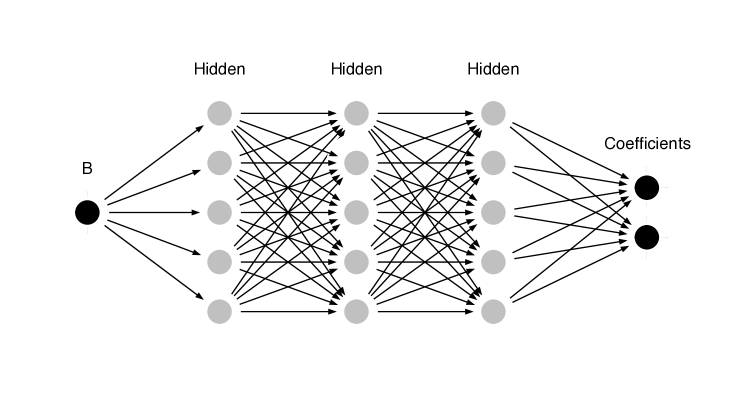
Figure 1: Three-layer neural network with one-dimensional input, hidden layer widths $5$, $5$, $5$ and output of length $2$.

Given the pairs $(B_{k},c(B_{k})),k=1,\ldots,M$, we minimize the functional (9) with respect to the parameters of the neural network. This is not a simple task, since it is a non-convex optimization problem. Fortunately, there are several standard methods for solving this optimization problem, based on stochastic gradient methods Goodfellow, Bengio, and Courville (2016), which are implemented in modern machine learning packages, like Tensorflow Abadi et al. (2015), and can be readily used. These methods have very good performance in practice. Among them, ADAM optimizer Kingma and Ba (2014) is one of the most efficient and we will use it.

IV Numerical results

IV.1 Single yield stress limit

As our first example, we consider a single-parameter case, namely, the parameter is the Bingham number $B$. We examine several types of cross-sections: square, rectangle, triangle, L-shaped domain. We randomly sample Bingham numbers from a uniform distribution on $[0,1]$ to obtain snapshots. Note that for all these domains the critical yield stress is smaller than $1$, so for $B>B_{crit}$ the velocity is equal to $0$, and snapshots, corresponding to these parameters do not provide any additional information. Such behavior is automatically captured by the proposed algorithm. For each domain, we collect the snapshot matrices, compute first POD basis functions, and corresponding coefficients. Singular values of the snapshot matrices decay very fast (see Figure 2), and $m=20$ provides very high accuracy of the approximation.

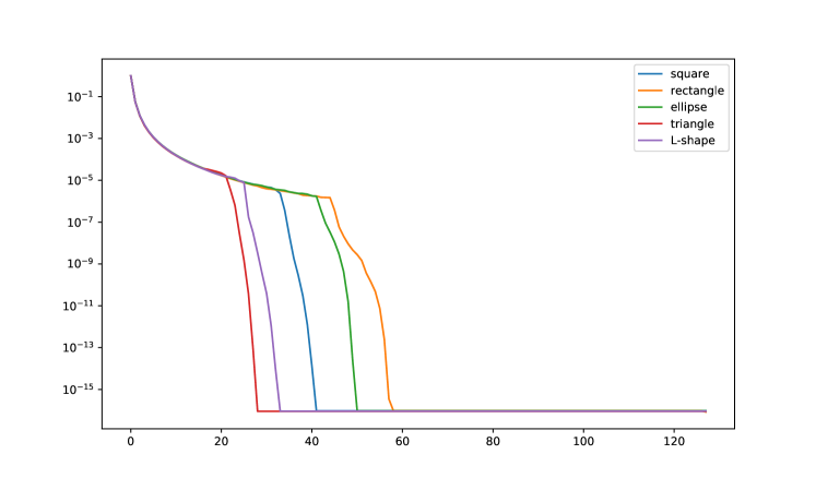
Figure 2: Decay of singular values of the snapshot matrices for different domains. Horizontal axis corresponds to the number of the singular value.

.

The first basis functions for different domains are shown on Figure 3.

As we see, the singular values decay very fast, thus it is sufficient to leave at most $m=20$ coefficients to get a good approximation. It is also interesting to look at the POD modes. The first $5$ POD modes and corresponding singular values are shown in Figure 3. Note that the first POD function has the structure “similar” to the typical flow pattern for each shape. This is an interesting topic for further research.

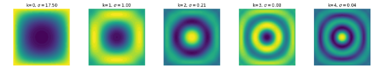
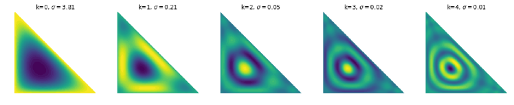
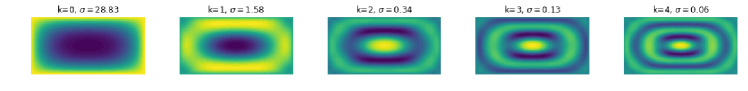
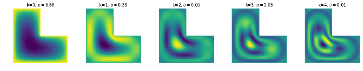
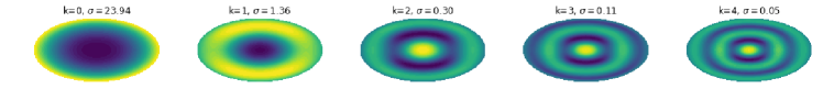
(a) (b) (c) (d) (e)

Figure 3: First 5 POD basis functions for different domains

To construct a neural network approximation for the mapping from $B$ to the first $K$ coefficients of the POD decomposition, we randomly split the dataset into test and train parts (33% test and 67% train), and learn a corresponding mapping. As an architecture of ANN we take $3$ hidden layers with $60,50,40$ hidden units, respectively and one output layer. As an optimizer, ADAM optimizer Kingma and Ba (2014) was used with default parameters. The relative error of approximation of coefficients on the test set for different domains is given in Table 1.

Domain	Relative error
square	0.006686
triangle	0.005700
L-shape	0.008667
rectangle	0.005344
ellipse	0.003489

Table 1: Relative error in the $L_{2}$ norm for the approximation of the first $K=200$ coefficients of the POD decomposition (test set).

IV.2 Non-homogenious yield stress limit

We consider the square case ($\Omega=[-\frac{1}{2},\frac{1}{2}]^{2}$), and a piecewise-constant yield stress limit. This corresponds to the flow of different fluids with different yield stress limits. This type of flows is rather common in practice: it includes such processes as lamination, coextrusion and deposition. For the model problem we consider a two-parameter problem with piecewise-constant $B(x_{1},x_{2})$:

$$B(x_{1},x_{2})=\begin{cases}B_{1}&x_{1}\leq 0,\\ B_{2}&x_{1}>0.\end{cases}$$

The parameters $B_{1}$ and $B_{2}$ vary from $0$ to $0.8$. For this problem we need to select more snapshots than for a single stress limit to get similar accuracy. We also have to sample two-dimensional points in the parameter space. To generate the POD basis, we compute $500$ snapshots with $B_{1}$ and $B_{2}$ generated using Halton quasi-random sequence generator Niederreiter (1992). The decay of singular values of the snapshot matrix is shown on Figure 4, and several first singular vectors are depicted on Figure 5.

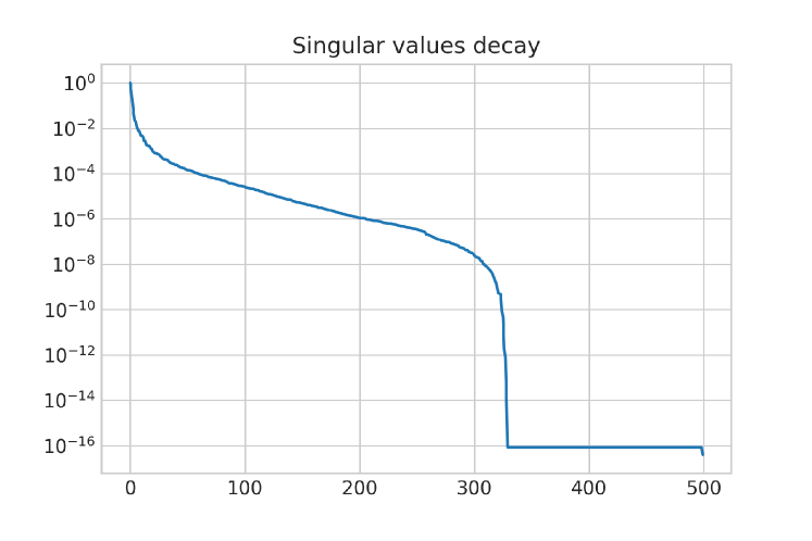
Figure 4: Decay of singular values for two-parameter problem

.

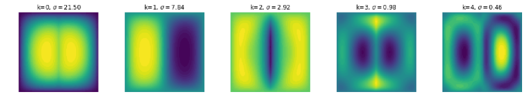
Figure 5: First five POD basis functions

.

Then we split the dataset randomly into training (67% points) and testing (33% points), and fit a fully connected ANN to map two input parameters ($B_{1}$ and $B_{2}$) to the first $20$ coefficients of the POD decomposition. As an architecture of ANN we take $3$ hidden layers with $60,50,40$ hidden units, respectively and one output layer.

As an optimizer we again use the Adam optimizer with default parameters. The relative error for the approximation on the test set is $0.008$.

The main benefit of using the reduced model is that computing the approximate solution for new $B_{1},B_{2}$ is very fast. The final model takes approximately 4 milliseconds to evaluate, whereas the full FEM model takes 45 seconds. The comparison of two solutions is given on Figure 6 for $B_{1}=0.25$ and $B_{2}=0.05$.

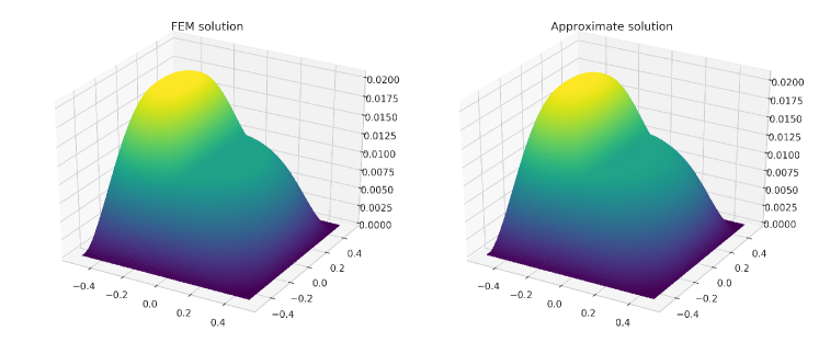
Figure 6: Comparison of FEM and approximate solution

.

IV.3 Flow rate vs pressure drop approximation

As an example of application of the reduced order model, we use it to compute the dependence of the flow rate on the pressure drop. To do that, we need to solve (1) for fixed $\tau_{s},\mu$ and varying pressure drop. This is equivalent to the computation of the solution of (2) with varying $B$. We can also compare the result computed from the approximant and the solution obtained from the full model. On Figure  7 the results are shown for different cross-sections and $B=0.1$, and on Figure 8 the results are shown for the non-homogenius yield stress case with different $B_{1}$ and $B_{2}$. The error behaviour is very similar to one-parameter case, so we omit it here.

It can be seen that in all cases the flow rate is approximated by the reduced model very accurately. The reduced order model is also much faster: the total computation time for $100$ different pressure drops was $0.05$ seconds for the reduced model, and $66$ seconds for the full model.

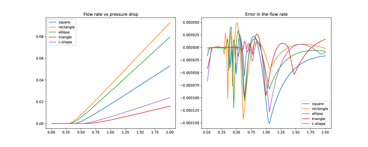
Figure 7: Flow rate vs pressure drop (left), difference between reduced and full model (right) for different cross-sections

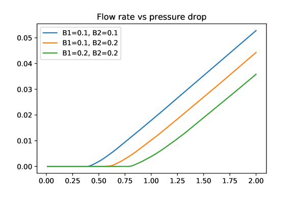
Figure 8: Flow rate vs pressure drop for non-homogenious case for different Bingham numbers

.

V Conclusions and future work

We have presented a general approach for the construction of reduced models of Bingham fluid flows in the simplest possible case — duct flow. Although being model, these flows share the main characteristics of more general cases. The proposed method is “easy to implement”: all the steps are automatic (generation of snapshots and fitting a neural network), but difficult to analyze: there is no guarantee that the approximated solution will share important properties of the original solution, such as positivity. This requires a separate study, as well as the application of the constructed reduced-order model to real-life design problems.

References

- Frigaard, Paso, and de Souza Mendes (2017) I. A. Frigaard, K. Paso, and P. de Souza Mendes, “Bingham’s model in the oil and gas industry,” Rheologica Acta 56, 259–282 (2017).
- Osiptsov (2017) A. Osiptsov, “Fluid mechanics of hydraulic fracturing: A review,” Journal of Petroleum Science and Engineering (2017).
- Guo et al. (2017) T. Guo, Z. Qu, F. Gong, and X. Wang, “Numerical simulation of hydraulic fracture propagation guided by single radial boreholes,” Energies 10, 1680 (2017).
- Shojaei, Taleghani, and Li (2014) A. Shojaei, A. Taleghani, and G. Li, “A continuum damage failure model for hydraulic fracturing of porous rocks,” International Journal of Plasticity 59, 199–212 (2014).
- Bunger and Lecampion (2017) A. Bunger and B. Lecampion, “Four critical issues for successful hydraulic fracturing applications,” Tech. Rep. (CRC Press, 2017).
- Li and Shojaei (2012) G. Li and A. Shojaei, “A viscoplastic theory of shape memory polymer fibres with application to self-healing materials,” Proc. R. Soc. A 468, 2319–2346 (2012).
- Saramito and Wachs (2017) P. Saramito and A. Wachs, “Progress in numerical simulation of yield stress fluid flows,” Rheologica Acta 56, 211–230 (2017).
- Mitsoulis and Tsamopoulos (2017) E. Mitsoulis and J. Tsamopoulos, “Numerical simulations of complex yield-stress fluid flows,” Rheologica Acta 56, 231–258 (2017).
- Ammar et al. (2006) A. Ammar, B. Mokdad, F. Chinesta, and R. Keunings, “A new family of solvers for some classes of multidimensional partial differential equations encountered in kinetic theory modeling of complex fluids,” Journal of Non-Newtonian Fluid Mechanics 139, 153–176 (2006).
- Chinesta et al. (2011) F. Chinesta, A. Ammar, A. Leygue, and R. Keunings, “An overview of the proper generalized decomposition with applications in computational rheology,” Journal of Non-Newtonian Fluid Mechanics 166, 578–592 (2011).
- Mosolov and Miasnikov (1965) P. Mosolov and V. Miasnikov, “Variational methods in the theory of the fluidity of a viscous-plastic medium,” Journal of Applied Mathematics and Mechanics 29, 545–577 (1965).
- Mosolov and Miasnikov (1966) P. Mosolov and V. Miasnikov, “On stagnant flow regions of a viscous-plastic medium in pipes,” Journal of Applied Mathematics and Mechanics 30, 841–854 (1966).
- Mosolov and Miasnikov (1967) P. Mosolov and V. Miasnikov, “On qualitative singularities of the flow of a viscoplastic medium in pipes,” Journal of Applied Mathematics and Mechanics 31, 609–613 (1967).
- Huilgol and You (2005) R. Huilgol and Z. You, “Application of the augmented Lagrangian method to steady pipe flows of Bingham, Casson and Herschel–Bulkley fluids,” Journal of Non-Newtonian Fluid Mechanics 128, 126–143 (2005).
- Saramito and Roquet (2001) P. Saramito and N. Roquet, “An adaptive finite element method for viscoplastic fluid flows in pipes,” Computer Methods in Applied Mechanics and Engineering 190, 5391–5412 (2001).
- Moyers-Gonzalez and A. (2004) M. A. Moyers-Gonzalez and F. I. A., “Numerical solution of duct flows of multiple visco-plastic fluids,” Journal of Non-Newtonian Fluid Mechanics 122, 227–241 (2004).
- Muravleva (2009) E. Muravleva, “Finite-difference schemes for the computation of viscoplastic medium flows in a channel,” Mathematical Models and Computer Simulations 1, 768–279 (2009).
- Walton and Bittleston (1991) I. C. Walton and S. H. Bittleston, “The axial flow of a Bingham plastic in a narrow eccentric annulus,” Journal of Fluid Mechanics 222, 39–60 (1991).
- Szabo and Hassager (1992) P. Szabo and O. Hassager, “Flow of viscoplastic fluids in eccentric annular geometries,” Journal of Non-Newtonian Fluid Mechanics 45, 149–169 (1992).
- Wachs (2007) A. Wachs, “Numerical simulation of steady Bingham flow through an eccentric annular cross-section by distributed Lagrange multiplier/fictitious domain and augmented Lagrangian methods,” Journal of Non-Newtonian Fluid Mechanics 142, 183–198 (2007).
- Muravleva and Muravleva (2009) E. A. Muravleva and L. V. Muravleva, “Unsteady flows of a viscoplastic medium in channels,” Mechanics of Solids 44, 792–812 (2009).
- Muravleva et al. (2010) L. Muravleva, E. Muravleva, G. Georgiou, and E. Mitsoulis, “Numerical simulations of cessation flows of a Bingham plastic with the augmented Lagrangian method,” Journal of Non-Newtonian Fluid Mechanics 164, 544–550 (2010).
- Roquet and Saramito (2008) N. Roquet and P. Saramito, “An adaptive finite element method for viscoplastic flows in a square pipe with stick–slip at the wall,” Journal of Non-Newtonian Fluid Mechanics 155, 101–115 (2008).
- Damianou et al. (2014) Y. Damianou, M. Philippou, G. Kaoullas, and G. Georgiou, “Cessation of viscoplastic Poiseuille flow with wall slip,” Journal of Non-Newtonian Fluid Mechanics 203, 24–37 (2014).
- Damianou and Georgiou (2014) Y. Damianou and G. Georgiou, “Viscoplastic Poiseuille flow in a rectangular duct with wall slip,” Journal of Non-Newtonian Fluid Mechanics 214, 88–105 (2014).
- Fortin and Glowinski (1983) M. Fortin and R. Glowinski, “The augmented Lagrangian method,” (1983).
- Logg, Mardal, and Wells (2012) A. Logg, K. Mardal, and G. Wells, Automated Solution of Differential Equations by the Finite Element Method (Springer, 2012).
- Kunisch and Volkwein (2002) K. Kunisch and S. Volkwein, “Galerkin proper orthogonal decomposition methods for a general equation in fluid dynamics,” SIAM Journal on Numerical analysis 40, 492–515 (2002).
- Peterson (1989) J. S. Peterson, “The reduced basis method for incompressible viscous flow calculations,” SIAM Journal on Scientific and Statistical Computing 10, 777–786 (1989).
- Lassila et al. (2014) T. Lassila, A. Manzoni, A. Quarteroni, and G. Rozza, “Model order reduction in fluid dynamics: challenges and perspectives,” in Reduced Order Methods for modeling and computational reduction (Springer, 2014) pp. 235–273.
- Goodfellow, Bengio, and Courville (2016) I. Goodfellow, Y. Bengio, and A. Courville, Deep Learning (MIT Press, 2016) http://www.deeplearningbook.org.
- Hornik, Stinchcombe, and White (1989) K. Hornik, M. Stinchcombe, and H. White, “Multilayer feedforward networks are universal approximators,” Neural networks 2, 359–366 (1989).
- Abadi et al. (2015) M. Abadi, A. Agarwal, P. Barham, E. Brevdo, Z. Chen, C. Citro, G. S. Corrado, A. Davis, J. Dean, M. Devin, S. Ghemawat, I. Goodfellow, A. Harp, G. Irving, M. Isard, Y. Jia, R. Jozefowicz, L. Kaiser, M. Kudlur, J. Levenberg, D. Mané, R. Monga, S. Moore, D. Murray, C. Olah, M. Schuster, J. Shlens, B. Steiner, I. Sutskever, K. Talwar, P. Tucker, V. Vanhoucke, V. Vasudevan, F. Viégas, O. Vinyals, P. Warden, M. Wattenberg, M. Wicke, Y. Yu, and X. Zheng, “TensorFlow: Large-scale machine learning on heterogeneous systems,” (2015), software available from tensorflow.org.
- Kingma and Ba (2014) D. Kingma and J. Ba, “ADAM: A method for stochastic optimization,” arXiv preprint arXiv:1412.6980 (2014).
- Niederreiter (1992) H. Niederreiter, Random number generation and quasi-Monte Carlo methods (SIAM, 1992).