Hyperfine-resolved rotation-vibration line list of ammonia (NH₃)

Abstract

A comprehensive, hyperfine-resolved rotation-vibration line list for the ammonia molecule (¹⁴NH₃) is presented. The line list, which considers hyperfine nuclear quadrupole coupling effects, has been computed using robust, first principles methodologies based on a highly accurate empirically refined potential energy surface. Transitions between levels with energies below $8000$ cm^-1 and total angular momentum $F\leq 14$ are considered. The line list shows excellent agreement with a range of experimental data and will significantly assist future high-resolution measurements of NH₃, both astronomically and in the laboratory.

1 Introduction

Ammonia (NH₃) has been detected in a wide variety of astrophysical environments and is an excellent molecular tracer because of its hyperfine structure. In local thermodynamic equilibrium (LTE) conditions, the relative line strengths of the hyperfine components provide a convenient way of deducing the optical depth (Mangum & Shirley, 2015), and subsequently characterizing the physical properties of molecular clouds (Ho & Townes, 1983). This approach avoids any of the complications associated with isotopologue comparisons, such as the assumption that one knows the isotopologue ratio, and there is no fractionation between the atomic ratio and molecular ratio. Anomalies between the observed and theoretically predicted hyperfine spectra are frequently observed in stellar cores, and whilst usually attributed to non-LTE conditions (Matsakis et al., 1977; Stutzki & Winnewisser, 1985) or systematic infall/outflow (Park, 2001), are still not well understood (Camarata et al., 2015). Accounting for hyperfine effects in spectroscopic observations is thus highly desirable and a detailed understanding of the underlying hyperfine patterns of rotation-vibration energy levels (Twagirayezu et al., 2016) can even benefit the interpretation of spectra measured with Doppler-limited resolution.

The hyperfine structure of the rovibrational energy levels is often described using effective Hamiltonian models (Hougen, 1972; Gordy & Cook, 1984), albeit even at 100 Hz precision (van Veldhoven et al., 2004), but the limited amount of hyperfine-resolved spectroscopic data means that these models become unreliable when extrapolating to spectral regions not sampled by the experimental data. More successful in their predictive power over extended frequency ranges are variational approaches, which intrinsically treat all resonant interactions between the rovibrational states. Such calculations are becoming increasingly useful in astronomical applications (Tennyson & Yurchenko, 2012; Tennyson et al., 2016), for example, variationally computed molecular line lists for methane (Yurchenko & Tennyson, 2014) and ammonia (Yurchenko et al., 2011a) were used to assign lines in the near-infrared spectra of late T dwarfs (Canty et al., 2015).

Recently, a generalized variational method for computing the nuclear quadrupole hyperfine effects in the rovibrational spectra of polyatomic molecules was reported by two of the authors (Yachmenev & Küpper, 2017). Utilizing this approach, we present a newly computed, hyperfine-resolved rotation-vibration line list for ¹⁴NH₃ applicable for high-resolution measurements in the microwave and near-infrared. Despite a reasonable amount of experimental and theoretical data on the quadrupole hyperfine structure of NH₃ having been reported in the literature, see Kukolich (1967); Dietiker et al. (2015); Augustovičová et al. (2016) and references therein, we are aware of only two extensive, hyperfine-resolved line lists (Coudert & Roueff, 2006; Yachmenev & Küpper, 2017). The work presented here is an improvement on both of these efforts and should greatly facilitate future measurements of NH₃, both astronomically and in the laboratory.

The paper is structured as follows: The line list calculations are described in Sec. 2 , including details on the potential energy surface (PES), dipole moment surface (DMS), electric field gradient (EFG) tensor surface, and variational nuclear motion computations. In Sec. 3 , the line list is presented along with comparisons against a range of experimental data. Concluding remarks are offered in Sec. 4 .

2 Line list calculations

Variational calculations employed the computer program TROVE (Yurchenko et al., 2007; Yachmenev & Yurchenko, 2015; Yurchenko et al., 2017) in conjunction with a recent implementation to treat hyperfine effects at the level of the nuclear quadrupole coupling (Yachmenev & Küpper, 2017), which is described by the interaction of the nuclear quadrupole moments with the electric field gradient (EFG) at the nuclei. Since the methodology of TROVE is well documented and hyperfine-resolved calculations on the rovibrational spectrum of NH₃ have been described (Yachmenev & Küpper, 2017), we summarize only the key details relevant for this work.

Initially, the spin-free rovibrational problem was solved for NH₃ to obtain the energies and wavefunctions for states up to $J=14$, where $J$ is the rotational angular momentum quantum number. The computational procedure for this stage is described in Yurchenko et al. (2011a), however, in this work we have used a new, highly accurate, empirically refined PES (Coles et al., 2018b). For solving the pure vibrational ($J=0$) problem, the size of the primitive vibrational basis set was truncated with the polyad number $P_{\mathrm{max}}=34$. The resulting basis of vibrational wavefunctions was then contracted to include states with energies up to $hc\cdot 20\,000$ cm^-1 ($h$ is the Planck constant and $c$ is the speed of light) relative to the zero-point energy. Multiplication with symmetry-adapted symmetric-top wavefunctions produced the final spin-free basis set for solving the $J>0$ rovibrational problem. The final rovibrational wavefunctions, combined with the nuclear spin functions, were used as a basis for solving the eigenvalue problem for the total spin-rovibrational Hamiltonian. The latter is composed of a sum of the diagonal representation of the pure rovibrational Hamiltonian and the non-diagonal matrix representation of the quadrupole coupling. The spin-rovibrational Hamiltonian is diagonal in $F$, the quantum number of the total angular momentum operator ${\bf F}={\bf J}+{\bf I}_{\rm N}$, which is the sum of the rovibrational ${\bf J}$ and the nuclear spin ${\bf I}_{\rm N}$ angular momentum operators.

Besides a PES, calculations require a dipole moment surface (DMS) for the computation of line strengths, and an EFG tensor surface. The ab initio EFG tensor surface at the quadrupolar nucleus ¹⁴N was generated on a grid of 4700 symmetry-independent molecular geometries of NH₃ using the coupled cluster method, CCSD(T), with all electrons correlated in conjunction with the augmented correlation-consistent core-valence basis set, aug-cc-pwCVQZ (Dunning, 1989; Kendall et al., 1992; Peterson & Dunning, 2002). Calculations utilized analytical coupled cluster energy derivatives (Scuseria, 1991) as implemented in the CFOUR program package (CFOUR, 2018). The elements of the EFG tensor were converted into a symmetry-adapted form in the D_3h(M) molecular symmetry group and represented by symmetry-adapted power series expansions up to sixth-order. Details of the representation and least-squares fitting procedure can be found in Yachmenev & Küpper (2017). Similarly, the ab initio DMS was calculated at the CCSD(T)/aug-cc-pCVQZ level of theory with all electrons correlated on the same grid of nuclear geometries as the EFG tensor. The least-squares fitting by analytical expansions was performed following the method described in Yurchenko et al. (2009) and Owens & Yachmenev (2018). A value of $eQ=20.44$ mb for the ¹⁴N nuclear quadrupole constant was used in calculations (Pyykkö, 2008). The optimized parameters of the EFG tensor surface along with the Fortran 90 functions to construct it are provided as supplementary material (Coles et al., 2018a).

The computed hyperfine-resolved rovibrational line list for ¹⁴NH₃ corresponds to wavelengths $\lambda>1.25$ µm and considers all transitions between states with energy $E\leq{}hc\cdot 8000$ cm^-1 relative to the zero-point level and $F\leq 14$, where $F=|J-I_{\mathrm{N}}|,\ldots,J+I_{\mathrm{N}}$ and $I_{\mathrm{N}}=1$. The format of the line list includes information on the initial and final rovibrational states involved in each transition such as its wavenumber in cm^-1, symmetry, and quantum numbers. The line list is provided as supplementary material (Coles et al., 2018a), along with programs to extract user-desired transition data.

3 Results

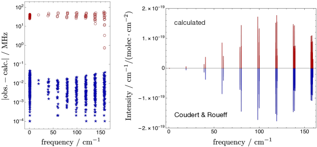
Figure 1: Discrepancies of the calculated transition frequencies of NH₃ relative to the experimental data for the ground $\nu_{0}$ vibrational state (Coudert & Roueff, 2006) (left panel) together with the calculated and observed spectrum (right panel). The errors in the rovibrational frequencies are plotted with red circles while the relative errors of the quadrupole splittings are plotted with blue stars.

Table 1: Discrepancies of the calculated transition frequencies (obs$-$calc) and intensities ($I$) with respect to the experimental data for the $\nu_{2}$ vibrational state of NH₃ (Belov et al., 1998). The relative errors (obs$-$calc/relative) are computed as quadrupole shifts with respect to the line with maximal intensity for each rovibrational band, i. e., lines with the same $J^{\prime\prime},k^{\prime\prime},\tau_{\text{inv}}^{\prime\prime}$ and $J^{\prime},k^{\prime},\tau_{\text{inv}}^{\prime}$, but different $F^{\prime\prime}$ and $F^{\prime}$. The calculated relative intensities (relative $I$/calc) are obtained by normalizing to the maximal observed intensity (relative $I$/obs) within each rovibrational band.

$J^{\prime}$	$k^{\prime}$	$\tau_{\text{inv}}^{\prime}$	$F^{\prime}$	$J^{\prime\prime}$	$k^{\prime\prime}$	$\tau_{\text{inv}}^{\prime\prime}$	$F^{\prime\prime}$	obs (MHz)	obs$-$calc (MHz)		relative $I$		absolute $I$
									absolute	relative	obs	calc
1	1	a	1	2	1	s	2	140140.794	606.842	-0.014	90.00	90.00	$7.532\times 10^{-25}$
1	1	a	1	2	1	s	1	140141.902	606.854	-0.003	30.00	30.00	$2.511\times 10^{-25}$
1	1	a	2	2	1	s	1	140142.163	606.478	-0.379	2.00	1.96	$1.637\times 10^{-26}$
1	1	a	2	2	1	s	3	140142.150	606.856	0.000	168.00	168.00	$1.406\times 10^{-24}$
1	1	a	2	2	1	s	2	140141.427	606.838	-0.018	30.00	30.00	$2.511\times 10^{-25}$
1	1	a	0	2	1	s	1	140143.503	606.862	0.006	40.00	40.00	$3.348\times 10^{-25}$
2	2	a	1	3	2	s	2	741789.155	595.343	0.000	252.00	252.00	$1.574\times 10^{-23}$
2	2	a	3	3	2	s	4	741788.397	595.343	0.000	540.00	540.00	$3.372\times 10^{-23}$
2	2	a	3	3	2	s	3	741788.399	595.344	0.001	46.67	46.67	$2.914\times 10^{-24}$
2	2	a	3	3	2	s	2	741788.403	595.349	0.006	1.33	1.18	$7.395\times 10^{-26}$
2	2	a	3	3	2	s	4	741788.398	595.344	0.001	540.00	540.00	$3.372\times 10^{-23}$
2	2	a	3	3	2	s	3	741788.388	595.333	-0.010	46.67	46.67	$2.914\times 10^{-24}$
2	2	a	3	3	2	s	2	741788.355	595.301	-0.042	1.33	1.18	$7.395\times 10^{-26}$
2	2	a	2	3	2	s	3	741787.015	595.324	-0.018	373.33	373.33	$2.331\times 10^{-23}$
2	2	a	2	3	2	s	2	741787.020	595.330	-0.012	46.67	46.67	$2.914\times 10^{-24}$
2	2	a	2	3	2	s	3	741787.019	595.328	-0.014	373.33	373.33	$2.331\times 10^{-23}$
2	2	a	2	3	2	s	2	741786.987	595.297	-0.045	46.67	46.67	$2.914\times 10^{-24}$
2	0	a	3	3	0	s	4	769710.287	576.907	0.000	540.00	540.00	$1.199\times 10^{-22}$
2	0	a	2	3	0	s	3	769710.281	576.932	0.026	373.33	373.35	$8.291\times 10^{-23}$
2	0	a	3	3	0	s	4	769710.289	576.909	0.002	540.00	540.00	$1.199\times 10^{-22}$
2	0	a	2	3	0	s	3	769710.277	576.928	0.022	373.33	373.35	$8.291\times 10^{-23}$
2	0	a	1	3	0	s	2	769710.000	576.890	-0.017	252.00	252.00	$5.596\times 10^{-23}$
2	0	a	3	3	0	s	3	769708.896	576.915	0.009	46.67	46.67	$1.036\times 10^{-23}$
2	0	a	3	3	0	s	2	769710.630	576.760	-0.147	1.33	1.18	$2.618\times 10^{-25}$
2	0	a	2	3	0	s	2	769712.123	576.885	-0.022	46.67	46.67	$1.036\times 10^{-23}$
2	1	a	3	3	1	s	3	762851.494	590.129	-0.037	46.67	21.78	$4.685\times 10^{-24}$
2	1	a	3	3	1	s	4	762852.624	590.166	0.000	252.00	252.00	$5.421\times 10^{-23}$
2	1	a	1	3	1	s	2	762852.624	590.163	-0.003	540.00	117.60	$2.530\times 10^{-23}$
2	1	a	3	3	1	s	2	762852.942	590.102	-0.064	1.33	0.55	$1.185\times 10^{-25}$
2	1	a	2	3	1	s	3	762852.209	590.160	-0.006	373.33	174.22	$3.748\times 10^{-23}$
2	1	a	2	3	1	s	2	762853.684	590.160	-0.006	46.67	21.78	$4.685\times 10^{-24}$
1	0	s	0	0	0	a	1	466243.620	-610.769	-0.007	4.00	4.31	$5.656\times 10^{-24}$
1	0	s	2	0	0	a	1	466245.605	-610.762	0.000	20.00	20.00	$2.625\times 10^{-23}$
1	0	s	1	0	0	a	1	466246.945	-610.740	0.022	12.00	12.93	$1.697\times 10^{-23}$

Table 2: Discrepancies of the calculated transition frequencies (obs$-$calc) with respect to the experimental data for the $\nu_{1}$, $\nu_{3}^{\pm 1}$, $2\nu_{4}^{0}$, $2\nu_{4}^{\pm 2}$ bands of NH₃ (Dietiker et al., 2015). The relative errors (obs$-$calc/relative) are computed as quadrupole shifts with respect to the line with maximal intensity for each rovibrational band, i. e., lines with the same $J^{\prime\prime},k^{\prime\prime},\tau_{\text{inv}}^{\prime\prime}$ and $J^{\prime},k^{\prime},\tau_{\text{inv}}^{\prime}$, but different $F^{\prime\prime}$ and $F^{\prime}$.

Vibr. level	$J^{\prime}$	$k^{\prime}$	$\tau_{\text{inv}}^{\prime}$	$F^{\prime}$	$J^{\prime\prime}$	$k^{\prime\prime}$	$\tau_{\text{inv}}^{\prime\prime}$	$F^{\prime\prime}$	obs (MHz)	obs$-$calc (MHz)		Intensity
										absolute	relative
$\nu_{1}$	1	1	a	1	2	1	s	2	101166502.618	-115.842	-0.009	$1.228\times 10^{-21}$
	1	1	a	2	2	1	s	2	101166503.217	-115.850	-0.016	$4.094\times 10^{-22}$
	1	1	a	1	2	1	s	1	101166503.787	-115.673	0.160	$4.094\times 10^{-22}$
	1	1	a	2	2	1	s	3	101166503.877	-115.833	0.000	$2.292\times 10^{-21}$
	1	1	a	0	2	1	s	1	101166505.196	-115.782	0.051	$5.458\times 10^{-22}$
	0	0	a	1	1	0	s	1	100580586.109	-76.131	-0.029	$2.249\times 10^{-21}$
	0	0	a	1	1	0	s	2	100580587.338	-76.102	0.000	$3.748\times 10^{-21}$
	0	0	a	1	1	0	s	0	100580589.137	-76.103	-0.001	$7.704\times 10^{-29}$
$\nu_{3}^{\pm 1}$	0	0	a	1	1	1	a	0	103686651.285	-279.126	-0.136	$2.231\times 10^{-29}$
	0	0	a	1	1	1	a	2	103686652.364	-278.989	0.000	$1.784\times 10^{-21}$
	0	0	a	1	1	1	a	1	103686652.874	-279.109	-0.119	$1.070\times 10^{-21}$
$2\nu_{4}^{0}$	0	0	a	1	1	0	s	1	97010274.474	148.905	0.164	$1.609\times 10^{-22}$
	0	0	a	1	1	0	s	0	97010277.532	148.929	0.188	$9.758\times 10^{-30}$
	0	0	a	1	1	0	s	2	97010275.524	148.741	0.000	$2.681\times 10^{-22}$
$2\nu_{4}^{\pm 2}$	0	0	a	1	1	1	a	0	97485902.014	670.652	-0.021	$1.194\times 10^{-29}$
	0	0	a	1	1	1	a	2	97485902.944	670.672	0.000	$3.540\times 10^{-22}$
	0	0	a	1	1	1	a	1	97485903.543	670.666	-0.006	$2.124\times 10^{-22}$

In Figure 1 , Table 1 and Table 2 , the predicted quadrupole hyperfine transition frequencies and intensities for NH₃ are compared with the available experimental data for the rotational transitions in the ground vibrational (Coudert & Roueff, 2006) and $\nu_{2}$ (Belov et al., 1998) states, and rovibrational transitions from the ground to the $\nu_{1}$, $\nu_{3}^{\pm 1}$, $2\nu_{4}^{0}$, and $2\nu_{4}^{\pm 2}$ vibrational states (Dietiker et al., 2015). A detailed survey of the available experimental and theoretical data for the quadrupole hyperfine structure of NH₃ can be found in Dietiker et al. (2015) and Augustovičová et al. (2016).

The absolute errors in the rovibrational frequencies are within the accuracy of the underlying PES (Coles et al., 2018b) and are reflective of what is achievable with variational nuclear motion calculations, i. e., sub-cm^-1 or better. To estimate the accuracy of the predicted quadrupole splittings and the underlying EFG surface, we have subtracted the respective error in the rovibrational frequency unperturbed from the quadrupole interaction effect for each transition. The resulting errors range from 0.1 to 46 kHz for the ground vibrational state (Figure 1 ) and from 1 to 64 kHz for the $\nu_{2}$ state (Table 1 ). Notably, two lines in Table 1 have inconsistently large deviations of 379 and 147 kHz from experiment, which do not correlate with the systematic errors of the calculation, but these lines have very small intensities and may have been misassigned. The root-mean-square errors for the ground vibrational and $\nu_{2}$ states are 9 kHz and 72 kHz, or 20 kHz if neglecting the two lines with irregular deviations, respectively. For other fundamental and overtone bands listed in Table 2 , the discrepancies are larger by up to 160 kHz, however, the estimated uncertainty of the experimental data is $\pm 100$ kHz (Dietiker et al., 2015), giving us confidence that the errors in our predictions are reasonably consistent. Overall, the agreement of the presented line list with experiment has improved in comparison to the previous theoretical study (Yachmenev & Küpper, 2017), which was based on an older PES (Yurchenko et al., 2011b) and an EFG tensor computed with a lower-level of ab initio theory.

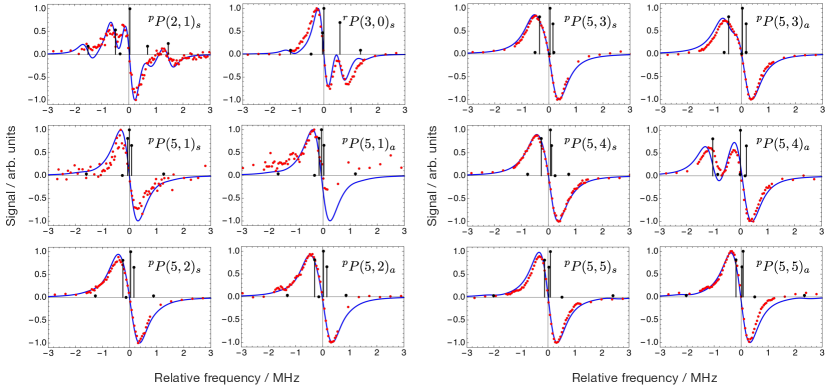
Figure 2: Comparison of the calculated (blue line) and observed (red dots) (Twagirayezu et al., 2016) saturation dip line shapes for the ${}^{\Delta K_{a}}\Delta J(J^{\prime\prime},K_{a}^{\prime\prime})_{\tau_{\text{inv}}^{\prime\prime}}$ transitions of the $\nu_{1}+\nu_{3}$ band of NH₃ ($\tau_{\text{inv}}^{\prime\prime}=s~{}\text{or}~{}a$ denotes symmetric or anti-symmetric inversion parity of the ground vibrational state, and ^′′ denotes the lower state). Black stems depict the calculated stick spectrum. The experimental and calculated intensities are normalized to the respective maximal values. The measured (calculated) zero-crossing wavenumbers, in cm^-1, are 6572.85349 (6572.81120) for ${}^{p}P(2,1)_{s}$, 6544.32154 (6544.28589) for ${}^{r}P(3,0)_{s}$, 6513.77250 (6513.73344) for ${}^{p}P(5,1)_{s}$, 6513.65575 (6513.59558) for ${}^{p}P(5,1)_{a}$, 6521.97101 (6521.93627) for ${}^{p}P(5,2)_{s}$, 6522.23374 (6522.25564) for ${}^{p}P(5,2)_{a}$, 6529.18969 (6529.18151) for ${}^{p}P(5,3)_{s}$, 6528.76857 (6528.74384) for ${}^{p}P(5,3)_{a}$, 6536.59280 (6536.55360) for ${}^{p}P(5,4)_{s}$, 6537.68063 (6538.22791) for ${}^{p}P(5,4)_{a}$, 6542.62402 (6542.63130) for ${}^{p}P(5,5)_{s}$, 6542.42400 (6542.44221) for ${}^{p}P(5,5)_{a}$.

Figure 2 shows comparisons with the sub-Doppler saturation dip spectroscopic measurements for the $\nu_{1}+\nu_{3}$ band of NH₃ (Twagirayezu et al., 2016; Sears, 2017). Saturation dip line shapes were calculated as the intensity-weighted sums of Lorentzian line shape derivatives (Axner et al., 2001) with a half-width-at-half-maximum (HWHM) of the absorption profile of 290 kHz and a HWHM-amplitude of the experimentally applied frequency-modulation dither of 150 kHz (Sears, 2017). A slightly larger HWHM was employed for the measured ${}^{p}P(5,K_{a}^{\prime\prime})$ transitions (Sears, 2017) and we have found a value of 500 kHz reproduces these line shapes well. Overall, the computed saturation dip profiles are in excellent agreement with experiment. Notably, in our previous theoretical study (Yachmenev & Küpper, 2017) we could not explain the observed double peak feature of the ${}^{p}P(5,4)_{a}$ transition and instead predicted a double peak structure in the ${}^{p}P(5,3)_{a}$ transition not seen in the experimental profile. This has now been rectified due to the use of a much improved and more reliable PES (Coles et al., 2018b) and the consideration of core-valence electron correlation in the calculation of the EFG tensor surface. Interestingly, the observed splitting in the ${}^{p}P(5,4)_{a}$ transition at 6777.63638 cm^-1 arises because the upper state is in fact a superposition of the three states $|J,k,\tau\rangle=|4,2,0\rangle$ of $\nu_{3}+\nu_{4}+3\nu_{2}$, $|4,3,1\rangle$ of $(\nu_{1}+\nu_{3})^{-}$ and $|4,3,0\rangle$ of $(\nu_{1}+\nu_{3})^{-}$ with approximately equal squared-coefficient contributions, where $\tau$ reflects the rotational parity defined as $(-1)^{\tau}$.

4 Conclusions

A new rotation-vibration line list for ¹⁴NH₃, which accounts for nuclear quadrupole hyperfine effects, has been presented. Comparisons with a range of experimental results showed excellent agreement, validating the computational approach taken. Notably, the new line list allowed to resolve line-shape discrepancies when compared with a previous hyperfine-resolved line list computed by two of the authors (Yachmenev & Küpper, 2017). Due to the variational approach taken, such improvements can be expected across the $0$–$8000$ cm^-1 region and can be attributed to the use of a highly accurate empirically refined PES and more rigorous electronic structure calculations for the EFG tensor surface. The line list contains detailed information, e. g., symmetry and quantum number labeling, for each transition, which will be extremely useful for future analysis of hyperfine-resolved ammonia spectra. Natural extensions to our calculations would be the consideration of a larger wavenumber range and higher energy level threshold, however, work in this direction will only be undertaken if there is a demand for such data.

The spectrum of ammonia is also of interest regarding a possible temporal or spatial variation of the proton-to-electron mass ratio $\mu$ (van Veldhoven et al., 2004). If any such variation has occurred, it would manifest as tiny but observable shifts in the frequencies of certain transitions. Constraints on a varying $\mu$ have been deduced using NH₃ in our Galaxy (Levshakov et al., 2010), in objects at high-redshift, for example, the system B0218$+$357 at redshift $z\sim 0.685$ (Flambaum & Kozlov, 2007; Murphy et al., 2008; Kanekar, 2011) or PKS1830$-$211 at $z\sim 0.886$ (Henkel et al., 2009), and are possible in high-precision laboratory setups (van Veldhoven et al., 2004; Cheng et al., 2016). Studying the mass sensitivity (Owens et al., 2015, 2016) of the hyperfine transitions could reveal promising spectral regions to guide future measurements of ammonia, ultimately leading to tighter constraints on drifting fundamental constants.

References

- Augustovičová et al. (2016) Augustovičová, L., Soldán, P., & Špirko, V. 2016, Astrophys. J., 824, 147, doi: 10.3847/0004-637x/824/2/147
- Axner et al. (2001) Axner, O., Kluczynski, P., & Lindberg, Å. M. 2001, J. Quant. Spectrosc. Radiat. Transfer, 68, 299, doi: 10.1016/s0022-4073(00)00032-7
- Belov et al. (1998) Belov, S., Urban, Š., & Winnewisser, G. 1998, J. Mol. Spectrosc., 189, 1, doi: 10.1006/jmsp.1997.7516
- Camarata et al. (2015) Camarata, M. A., Jackson, J. M., & Chambers, E. 2015, Astrophys. J., 806, 74, doi: 10.1088/0004-637x/806/1/74
- Canty et al. (2015) Canty, J. I., Lucas, P. W., Yurchenko, S. N., et al. 2015, Mon. Not. R. Astron. Soc., 450, 454, doi: 10.1093/mnras/stv586
- CFOUR (2018) CFOUR. 2018, Coupled-Cluster techniques for Computational Chemistry, a quantum chemical program package written by J. F. Stanton, J. Gauss, M. E. Harding, and P. G. Szalay with contributions from A. A. Auer, R. J. Bartlett, U. Benedikt, C. Berger, D. E. Bernholdt, Y. J. Bomble, L. Cheng, O. Christiansen, M. Heckert, O. Heun, C. Huber, T.-C. Jagau, D. Jonsson, J. Jusélius, K. Klein, W. J. Lauderdale, D. A. Matthews, T. Metzroth, L. A. Mück, D. P. O’Neill, D. R. Price, E. Prochnow, C. Puzzarini, K. Ruud, F. Schiffmann, W. Schwalbach, S. Stopkowicz, A. Tajti, J. Vázquez, F. Wang, J. D. Watts, and the integral packages MOLECULE (J. Almlöf and P. R. Taylor), PROPS (P. R. Taylor), ABACUS (T. Helgaker, H. J. Aa. Jensen, P. Jørgensen, and J. Olsen), and ECP routines by A. V. Mitin and C. van Wüllen. For the current version, see http://www.cfour.de.
- Cheng et al. (2016) Cheng, C., van der Poel, A. P. P., Jansen, P., et al. 2016, Phys. Rev. Lett., 117, 253201, doi: 10.1103/PhysRevLett.117.253201
- Coles et al. (2018a) Coles, P., Owens, A., Küpper, J., & Yachmenev, A. 2018a, Supplementary material: Hyperfine-resolved rotation-vibration line list of ammonia (NH3) [Data set], doi: 10.5281/zenodo.1414346. https://doi.org/10.5281/zenodo.1414346
- Coles et al. (2018b) Coles, P. A., Ovsyannikov, R. I., Polyansky, O. L., Yurchenko, S. N., & Tennyson, J. 2018b, J. Quant. Spectrosc. Radiat. Transf., 219, 199, doi: 10.1016/j.jqsrt.2018.07.022
- Coudert & Roueff (2006) Coudert, L. H., & Roueff, E. 2006, Astron. Astrophys., 449, 855, doi: 10.1051/0004-6361:20054136
- Dietiker et al. (2015) Dietiker, P., Miloglyadov, E., Quack, M., Schneider, A., & Seyfang, G. 2015, J. Chem. Phys., 143, 244305, doi: 10.1063/1.4936912
- Dunning (1989) Dunning, T. H. 1989, J. Chem. Phys., 90, 1007
- Flambaum & Kozlov (2007) Flambaum, V. V., & Kozlov, M. G. 2007, Phys. Rev. Lett., 98, 240801, doi: 10.1103/PhysRevLett.98.240801
- Gordy & Cook (1984) Gordy, W., & Cook, R. L. 1984, Microwave Molecular Spectra, 3rd edn. (New York, NY, USA: John Wiley & Sons)
- Henkel et al. (2009) Henkel, C., Menten, K. M., Murphy, M. T., et al. 2009, Astron. Astrophys., 500, 725, doi: 10.1051/0004-6361/200811475
- Ho & Townes (1983) Ho, P. T. P., & Townes, C. H. 1983, Ann. Rev. Astron. Astrophys., 21, 239
- Hougen (1972) Hougen, J. T. 1972, J. Chem. Phys., 57, 4207, doi: 10.1063/1.1678050
- Kanekar (2011) Kanekar, N. 2011, Astrophys. J. Lett., 728, L12, doi: 10.1088/2041-8205/728/1/l12
- Kendall et al. (1992) Kendall, R. A., Dunning, Jr., T. H., & Harrison, R. J. 1992, J. Chem. Phys., 96, 6796, doi: 10.1063/1.462569
- Kukolich (1967) Kukolich, S. G. 1967, Phys. Rev., 156, 83, doi: 10.1103/PhysRev.156.83
- Levshakov et al. (2010) Levshakov, S. A., Lapinov, A. V., Henkel, C., et al. 2010, Astron. Astrophys., 524, A32, doi: 10.1051/0004-6361/201015332
- Mangum & Shirley (2015) Mangum, J. G., & Shirley, Y. L. 2015, Publ. Astron. Soc. Pac., 127, 266, doi: 10.1086/680323
- Matsakis et al. (1977) Matsakis, D. N., Brandshaft, D., Chui, M. F., et al. 1977, Astrophys. J. Lett., 214, L67, doi: 10.1086/182445
- Murphy et al. (2008) Murphy, M. T., Flambaum, V. V., Muller, S., & Henkel, C. 2008, Science, 320, 1611, doi: 10.1126/science.1156352
- Owens & Yachmenev (2018) Owens, A., & Yachmenev, A. 2018, J. Chem. Phys., 148, 124102, doi: 10.1063/1.5023874
- Owens et al. (2016) Owens, A., Yurchenko, S. N., Thiel, W., & Špirko, V. 2016, Phys. Rev. A, 93, 052506, doi: 10.1103/PhysRevA.93.052506
- Owens et al. (2015) Owens, A., Yurchenko, S. N., Thiel, W., & Špirko, V. 2015, Mon. Not. R. Astron. Soc., 450, 3191, doi: 10.1093/mnras/stv869
- Park (2001) Park, Y.-S. 2001, Astron. Astrophys., 376, 348, doi: 10.1051/0004-6361:20010933
- Peterson & Dunning (2002) Peterson, K. A., & Dunning, T. H. 2002, J. Chem. Phys., 117, 10548, doi: 10.1063/1.1520138
- Pyykkö (2008) Pyykkö, P. 2008, Mol. Phys., 106, 1965, doi: 10.1080/00268970802018367
- Scuseria (1991) Scuseria, G. E. 1991, J. Chem. Phys., 94, 442, doi: 10.1063/1.460359
- Sears (2017) Sears, T. J. 2017, private communication
- Stutzki & Winnewisser (1985) Stutzki, J., & Winnewisser, G. 1985, Astron. Astrophys., 144, 13
- Tennyson & Yurchenko (2012) Tennyson, J., & Yurchenko, S. N. 2012, Mon. Not. R. Astron. Soc., 425, 21, doi: 10.1111/j.1365-2966.2012.21440.x
- Tennyson et al. (2016) Tennyson, J., Yurchenko, S. N., Al-Refaie, A. F., et al. 2016, J. Mol. Spectrosc., 327, 73, doi: 10.1016/j.jms.2016.05.002
- Twagirayezu et al. (2016) Twagirayezu, S., Hall, G. E., & Sears, T. J. 2016, J. Chem. Phys., 145, 144302, doi: 10.1063/1.4964484
- van Veldhoven et al. (2004) van Veldhoven, J., Küpper, J., Bethlem, H. L., et al. 2004, Eur. Phys. J. D, 31, 337, doi: 10.1140/epjd/e2004-00160-9
- Yachmenev & Küpper (2017) Yachmenev, A., & Küpper, J. 2017, J. Chem. Phys., 147, 141101, doi: 10.1063/1.5002533
- Yachmenev & Yurchenko (2015) Yachmenev, A., & Yurchenko, S. N. 2015, J. Chem. Phys., 143, 014105, doi: 10.1063/1.4923039
- Yurchenko et al. (2011a) Yurchenko, S. N., Barber, R. J., & Tennyson, J. 2011a, Mon. Not. R. Astron. Soc., 413, 1828, doi: 10.1111/j.1365-2966.2011.18261.x
- Yurchenko et al. (2011b) Yurchenko, S. N., Barber, R. J., Tennyson, J., Thiel, W., & Jensen, P. 2011b, J. Mol. Spectrosc., 268, 123, doi: 10.1016/j.jms.2011.04.005
- Yurchenko et al. (2009) Yurchenko, S. N., Barber, R. J., Yachmenev, A., et al. 2009, J. Phys. Chem. A, 113, 11845, doi: 10.1021/jp9029425
- Yurchenko & Tennyson (2014) Yurchenko, S. N., & Tennyson, J. 2014, Mon. Not. R. Astron. Soc., 440, 1649, doi: 10.1093/mnras/stu326
- Yurchenko et al. (2007) Yurchenko, S. N., Thiel, W., & Jensen, P. 2007, J. Mol. Spectrosc., 245, 126, doi: 10.1016/j.jms.2007.07.009
- Yurchenko et al. (2017) Yurchenko, S. N., Yachmenev, A., & Ovsyannikov, R. I. 2017, J. Chem. Theory Comput., 13, 4368, doi: 10.1021/acs.jctc.7b00506