Predictive Collective Variable Discovery with Deep Bayesian Models

Abstract

Preprint - accepted and published in The Journal of Chemical Physics 2019 150:2; https://doi.org/10.1063/1.5058063.
Extending spatio-temporal scale limitations of models for complex atomistic systems considered in biochemistry and materials science necessitates the development of enhanced sampling methods. The potential acceleration in exploring the configurational space by enhanced sampling methods depends on the choice of collective variables (CVs). In this work, we formulate the discovery of CVs as a Bayesian inference problem and consider the CVs as hidden generators of the full-atomistic trajectory. The ability to generate samples of the fine-scale atomistic configurations using limited training data allows us to compute estimates of observables as well as our probabilistic confidence on them. The methodology is based on emerging methodological advances in machine learning and variational inference. The discovered CVs are related to physicochemical properties which are essential for understanding mechanisms especially in unexplored complex systems. We provide a quantitative assessment of the CVs in terms of their predictive ability for alanine dipeptide (ALA-2) and ALA-15 peptide.

I Introduction

Molecular dynamics (MD) simulations, in combination with prevalent algorithmic enhancements and tremendous progress in computational resources, have contributed to new insights into mechanisms and processes present in physics, chemistry, biology and engineering. However, their applicability in systems of practical relevance poses insurmountable computational difficulties Perilla et al. (2015); Koutsourelakis, Zabaras, and Girolami (2016). For example, the simulation of $M=10^{5}$ atoms over a time horizon of a mere $T\approx 10^{-4}~{}\textnormal{s}$ with a time step of $\Delta t=10^{-15}~{}\textnormal{s}$ implies a computational time of one year Barducci, Bonomi, and Parrinello (2011a). A rugged free-energy surface and configurations separated by high free-energy barriers lead to unobserved conformations even in very long simulations.

Enhanced sampling methods Pietrucci and Andreoni (2011) provide a framework for accelerating the exploration of the configurational space Ferguson et al. (2011a); Zheng, Rohrdanz, and Clementi (2013); Valsson and Parrinello (2014); Chen and Ferguson (2018); Chen and Tuckerman (2018); Mitsutake, Mori, and Okamoto (2013); Bierig and Chernov (2016). Those methods rely on the existence of a lower-dimensional representation of the atomistic detail. Lower-dimensional system variables (reaction coordinates), capture the characteristics of the system, allow us to understand relevant processes and conformational changes Luque and Barril (2012), and can enable guided and enhanced MD simulations. Reaction coordinates provide quantitative understanding of macromolecular motion, whereas order parameters are of qualitative nature as discussed in [Rohrdanz, Zheng, and Clementi, 2013]. In the following, we use the term collective variables (CVs), combining the quantitative and qualitative properties of reaction coordinates and order parameters, respectively. Refs. [Pietrucci and Andreoni, 2011; Rohrdanz, Zheng, and Clementi, 2013] review the challenges in the exploration of the free-energy landscape and the identification of “good” collective variables.

Adding an appropriate biasing potential or force, based on CVs, results into an accelerated exploration of the configurational space Rohrdanz, Zheng, and Clementi (2013). Such algorithms might employ a constant bias term (e.g. umbrella sampling Torrie and Valleau (1977), hyperdynamics Voter (1997), accelerated MD Hamelberg, Mongan, and McCammon (2004), etc.) or a time-dependent one (e.g. local elevation Huber, Torda, and van Gunsteren (1994), conformational flooding Grubmüller (1995), metadynamics Laio and Parrinello (2002); Barducci, Bonomi, and Parrinello (2011b, a), adaptive biasing force Darve, Rodríguez-Gómez, and Pohorille (2008); Hénin et al. (2010), etc.). The crucial ingredient for almost all of the aforementioned algorithms is the right choice of the collective variables. The potential benefit and justification of enhanced sampling algorithms strongly depend on the quality of the collective variables as comprehensively elaborated in [Pietrucci, 2017; Pan et al., 2014; Fu, Oliveira, and Pfaendtner, 2017]. Physical intuition, experience gathered from previous simulation as well as quantitative methods for dimensionality reduction (e.g. by utilizing principal component analysis Hotelling (1933) (PCA)), potentially support the choice of reasonable collective variables. For complex materials-design problems and large-scale biochemical processes, complexity exceeds our intuition and the question of “good” collective variables remains unanswered. Enhanced sampling methods employing inappropriate collective variables can be outperformed by brute force MD simulations McGibbon, Husic, and Pande (2017). Thus, the identification of collective variables or reaction coordinates poses an important and difficult problem.

A systematic, robust, and general approach is needed for the discovery of lower-dimensional representations. Recent developments in dimensionality reduction methods provide a systematic strategy for discovering CVs Rohrdanz, Zheng, and Clementi (2013). For completeness, we give a brief overview of significant tools addressing CV discovery and dimensionality reduction in the context of molecular systems. An early study Amadei, Linssen, and Berendsen (1993) found a steep decay in the eigenvalues of peptide trajectories indicating the existence of a low-dimensional representation that is capable of capturing essential physics. This study is based on PCA Pearson (1901); Hotelling (1933) which identifies a linear coordinate transformation for best capturing the variance. However, the linear coordinate transformations employed merely describe local fluctuations in the context of peptide trajectories. Multidimensional scaling (MDS) Troyer and Cohen (1995); Härdle and Simar (2007) identifies a lower-dimensional embedding such that pairwise distances (e.g. root-mean-square deviation (RMSD)) between atomistic configurations are best preserved. Sketch-map Ceriotti, Tribello, and Parrinello (2011) focuses on preserving “middle” ranged RMSD between trajectory pairs. Middle ranged RMSD pairs are the most relevant for observing pertinent behavior of the system Ceriotti, Tribello, and Parrinello (2011). Isometric feature map or ISOMAP Tenenbaum, Silva, and Langford (2000) follows a similar idea of preserving geodesic distances. The aforementioned methods require dense sampling and encounter problems if the training data is non-uniformly distributed Rohrdanz et al. (2011); Balasubramanian and Schwartz (2002); Donoho and Grimes (2003). Furthermore, we note that those methods involve a mapping from the atomistic configurations to the CVs whereas predictive tasks require a generative mapping from the CVs to the atomistic configuration.

Another group of non-linear dimensionality reduction methods follows the idea of approximating the eigenfunctions of the backward Fokker-Plank operator Risken and Frank (1996) by identifying eigenvalues and eigenvectors of transition kernels. The employed kernels resemble transition probabilities between configurations that we aim to preserve. For example, the diffusion map Coifman et al. (2005a, b); Ferguson et al. (2011b) retains the diffusion distance by the identified coordinates for dynamic Nadler et al. (2006) and stochastic systems Coifman et al. (2008). A variation of diffusion maps exploits locally scaled diffusion maps (LSDMap) Rohrdanz et al. (2011) which calculate the transition probabilities between two configurations, utilizing the RMSD instead of an Euclidean distance. An additional local scale parameter, indicating the distance around a specific configuration presumably could be well approximated by a low-dimensional hyperplane tangent. LSDMap is applied in [A. Rohrdanz et al., 2014] and enhances the exploration of the configurational space as shown in [Zheng et al., 2013]. More recent approaches to collective variable discovery work under a common variational approach for conformation dynamics (VAC) Noé and Nüske (2013) and employ a combination of basis functions for defining the eigenfunctions to the backward Fokker-Planck operator. One approach under VAC was developed in the context of metadynamics Laio and Parrinello (2002) combining ideas from time-lagged independent component analysis and well-tempered metadynamics McCarty and Parrinello (2017). Further developments have focused on alternate distance metrics, relying either on a kinetic distance which measures how slowly configurations interconvert Noé and Clementi (2015), or on the commute distance Noé, Banisch, and Clementi (2016) which provides an extension (arising by integration) of the former.

Several methods rely on the estimation of the eigenvectors of transitions matrices which is an expensive task in terms of computational cost. The need for “large” training datasets (e.g. $10\,000$ datapoints are required for robustness of the results  Rohrdanz, Zheng, and Clementi (2013)) limits the applicability of these methods to less complex systems. We refer to [Duan et al., 2013] for a critical review and comparison of the various methodologies mentioned before.

In this work, we propose a data-driven reformulation of the identification of CVs under the paradigm of probabilistic (Bayesian) inference. The methodology implies a generative model, considering CVs as lower-dimensional (latent) generators Jordan (1999) of the full atomistic trajectory. The focus furthermore is on problems where limited atomistic training data are available that prohibit the accurate calculation of statistics for quantities of interest. Our approach is to compute an approximation of the underlying probabilistic distribution of the data. We then use this approximate distribution in a generative manner to perform accurate Monte Carlo estimation of the quantities of interest. To account for the limited information provided by small size training datasets, epistemic uncertainties on quantities of interest are also computed within the Bayesian paradigm.

In the context of coarse-graining atomistic systems, latent variable models have been introduced in [Schöberl, Zabaras, and Koutsourelakis, 2017; Felsberger and Koutsourelakis, 2018]. We optimize a flexible non-linear mapping between CVs and atomistic coordinates which implicitly specifies the meaning of the CVs. The identified CVs provide physical/chemical insight into the characteristics of the considered system. In the proposed model, the posterior distribution of the CVs for a given atomistic data point is computed. This posterior provides a pre-image of the atomistic representation in the lower-dimensional latent space. We utilize recent developments in machine learning and deep Bayesian modeling (Auto-Encoding Variational BayesKingma and Welling (2013); Rezende, Mohamed, and Wierstra (2014)). While typically deep learning models rely on huge amounts on data, we demonstrate the robustness of the proposed methodology considering only small and highly-variable datasets (e.g. $50$ data points compared to $10\,000$ as required in the aforementioned methods). The proposed strategy requires significantly less data as compared to MDS Troyer and Cohen (1995); Härdle and Simar (2007), ISOMAP Tenenbaum, Silva, and Langford (2000), and diffusion map Coifman et al. (2005a, b); Nadler et al. (2006) and simultaneously enables the quantification of uncertainties arising from limited data. We also discuss how additional datapoints can be readily incorporated by efficiently updating the previously trained model.

Apart from the possibility of utilizing the discovered CVs for dimensionality reduction and enhanced sampling, we exploit them for predictive purposes i.e. for generating new atomistic configurations and estimating macroscopic observables. One could draw similarities between the identification of CVs and the problem of identifying a good coarse-grained representation Kmiecik et al. (2016); Noid et al. (2007); Shell (2008); Peter and Kremer (2009); Trashorras and Tsagkarogiannis (2010); Kalligiannaki et al. (2012); Harmandaris et al. (2016); Bilionis and Zabaras (2013); Dama et al. (2013); Noid (2013); Foley, Shell, and Noid (2015); Schöberl, Zabaras, and Koutsourelakis (2017); Langenberg et al. (2018). In addition, rather than solely obtaining point estimates of observables, the Bayesian framework adopted provides whole distributions which capture the epistemic uncertainty. This uncertainty propagates in the form of error bars around the predicted observables.

Several recent publications focus on similar problems Hernández et al. (2017); Wehmeyer and Noé (2018); Sultan, Wayment-Steele, and Pande (2018). The present work clearly differs from [Sultan, Wayment-Steele, and Pande, 2018] where the data is provided in a pre-processed form of sine and cosine backbone dihedral angles, i.e. not as the full-atom configurations. The approach in [Wehmeyer and Noé, 2018] utilizes a pre-reduced representation of heavy atom positions as training data. While this is valid, it necessitates physical insight which might be not available for unexplored complex chemical compounds. In contrast, we rely on training data represented as Cartesian coordinates comprising all atoms of the considered system. We do not consider any physically- or chemically-motivated transformation nor do we perform any preprocessing of the dataset. Instead, we reveal, given the dimensionality of the CVs, important characteristics (i.e. dihedral angles, heavy atom positions) or less relevant fluctuations (noise) from the full atomistic picture. This work is also distinguished by following throughout a formalism based on Bayesian Learning. Instead of adopting or designing optimization objectives or loss functions, we consistently work within a Bayesian framework where the objective naturally arises. Furthermore, this readily allows us to make use of sparsisty-inducing priors which reveal parsimonious features. The work of [Chen and Ferguson, 2018] is based on auto-associative artificial neural networks (autoencoders) which allow the encoding and reconstruction of atomistic configurations given an input datum. Ref. [Chen and Ferguson, 2018] relies on reduced Cartesian coordinates in the form of backbone atoms which induces information loss. In addition, the focus in [Chen and Ferguson, 2018] is on CV discovery and enhanced sampling whereas we focus on CV discovery and obtaining a predictive model accounting for epistemic uncertainty.

The structure of the rest of the paper is as follows. Section II presents the basic model components, the use of Variational Autoencoders  (VAEsKingma and Welling (2013)) in the CV discovery, and provides details on the learning algorithms employed. Numerical evidence of the capabilities of the proposed framework is provided in Section III. We identify CVs for alanine dipeptide and show the correlation between the discovered CVs and the dihedral angles. We furthermore assess the predictive quality of the discovered CVs and estimate observables augmented by credible intervals. We show the dependence of credible intervals on the amount of training data. We also present the results of a similar analysis for a more complex and higher-dimensional molecule, i.e. the ALA-15 peptide. Finally, Section IV summarizes the key findings of this paper and provides a brief discussion on potential extensions.

II Methods

After introducing the main notational convention in the context of equilibrium statistical mechanics, this section is devoted to the key concepts of generative latent variable models and variational inference Beal (2003) with emphasis on the identification of collective variables in atomistic systems.

II.1 Equilibrium statistical mechanics

We denote the coordinates of atoms of a molecular ensemble as $\bm{x}\in\mathcal{M}_{\text{f}}\subset\mathbb{R}^{n_{\text{f}}}$, with $n_{\text{f}}=\dim(\bm{x})$. The coordinates $\bm{x}$ follow the Boltzmann-Gibbs density,

$$p_{\text{target}}(\bm{x})=\frac{1}{Z(\beta)}e^{-\beta U(\bm{x})},$$ (1)

with the interatomic potential $U(\bm{x})$, $\beta=\frac{1}{k_{b}T}$ where $k_{b}$ is the Boltzmann constant and $T$ the temperature. The normalization constant is given as $Z(\beta)=\int_{\mathcal{M}_{\text{f}}}\exp\{-\beta U(\bm{x})\}~{}d\bm{x}$. MD simulations Alder and Wainwright (1959), or Monte-Carlo-based methods Landau and Binder (2005) allow us to obtain samples from the distribution defined in Eq. (1). In the following, we assume that a dataset, $\bm{X}=\{\bm{x}^{(i)}\}_{i=1}^{N}$, has been collected, where $\bm{x}^{(i)}\sim p_{\text{target}}(\bm{x})$. $N$ denotes the amount of data points considered. The dataset $\bm{X}$ will be used for training the generative model to be introduced in the sequel. The underlying assumption in this work is that the size of the available training dataset $\bm{X}$ is small and not sufficient to compute directly statistics of observables. Our focus is thus on deriving an approximation to the distribution in Eq. (1) from which, in a computationally inexpensive manner, one can sample sufficient realizations of $\bm{x}$ to allow probabilistic estimates of observables.

As elaborated in [Rohrdanz, Zheng, and Clementi, 2013], the collection of a dataset $\bm{X}$ that sufficiently captures the configurational space constitutes a difficult problem of its own. Hampered by free-energy barriers, a MD simulation is not guaranteed to visit all conformations of an atomistic system within a finite simulation time. The discovery of CVs can facilitate the development of enhanced sampling methods Pietrucci (2017); Laio and Parrinello (2002); Barducci, Bonomi, and Parrinello (2011a) to address the efficient exploration of the configurational space.

This study considers systems in equilibrium for a given constant temperature $T$ and consequently constant $\beta$. Optimally, the CVs discovered should be suitable for a range of temperatures Fu, Oliveira, and Pfaendtner (2017).

II.2 Probabilistic generative models

Deep learning LeCun, Bengio, and Hinton (2015) integrated with probabilistic modeling Ghahramani (2015) has impacted many research areas von der Linden, Dose, and von Toussaint (2014). In this paper, we emphasize a subset of these models referred to as probabilistic generative models Jordan (1999); Ng and Jordan (2002).

The objective is to identify CVs associated with relevant configurational changes of the system of interest. We consider CVs as hidden (low-dimensional) generators, giving rise to the observed atomistic configurations $\bm{x}$ MacKay (2003). Extending the variable space of atomistic coordinates $\bm{x}$ by latent CVs denoted as $\bm{z}\in\mathcal{M}_{\text{CV}}\subset\mathbb{R}^{n_{\text{CV}}}$, with $n_{\text{CV}}=\dim(\bm{z})$ and $\dim(\bm{z})\ll\dim(\bm{x})$, allows us to define a joint distribution over the observed data $\bm{x}$ and latent CVs Jordan (1999); Bishop (1999) $p(\bm{x},\bm{z})$. The joint distribution $p(\bm{x},\bm{z})$ is written as,

$$p(\bm{x},\bm{z})=p(\bm{x}|\bm{z})~{}p(\bm{z}).$$ (2)

In Eq. (2), $p(\bm{z})$ prescribes the distribution of the CVs and $p(\bm{x}|\bm{z})$ represents the conditional probability of the full atomistic coordinates $\bm{x}$ given their latent representation $\bm{z}$. The probabilistic connection between the latent CVs $\bm{z}$ and the atomistic representation $\bm{x}$ implicitly defines the meaning of the CVs.

Marginalizing the joint representation of Eq. (2) with respect to the CVs leads to $p(\bm{x})$,

$$p(\bm{x})=\int_{\mathcal{M}_{\text{CV}}}p(\bm{x},\bm{z})~{}d\bm{z}=\int_{\mathcal{M}_{\text{CV}}}p(\bm{x}|\bm{z})~{}p(\bm{z})~{}d\bm{z}.$$ (3)

Equation (3) provides a generative model for the atomistic configurations $\bm{x}$ and will be utilized as an efficient estimator for observables of the atomistic system. Standard autoencoders in the context of CV discovery Chen and Ferguson (2018) do not yield a probabilistic, predictive model which is the focus of this work. With appropriate selection of $p(\bm{z})$ and $p(\bm{x}|\bm{z})$, the resulting predictive distribution $p(\bm{x})$ should resemble the atomistic reference $p_{\text{target}}(\bm{x})$ in Eq. (1). In order to quantify the closeness of the approximating distribution $p(\bm{x})$ and the actual distribution $p_{\text{target}}(\bm{x})$, a distance measure is employed. The KL-divergence is one possibility out of the family of $\alpha$-divergencesCichocki and Amari (2010); Cha (2007) measuring the similarity between ${{red}p_{\text{target}}}(\bm{x})$ and $p(\bm{x})$. The non-negative valued KL-divergence is zero if and only if the two distributions coincide, which leads to the minimization objective with respect to $p(\bm{x})$ of the following form:

$$D_{KL}(p_{\text{target}}(\bm{x})||p(\bm{x}))= -\int_{\mathcal{M}_{\text{f}}}p_{\text{target}}(\bm{x})\log\frac{p(\bm{x})}{p_{\text{target}}(\bm{x})}~{}d\bm{x}$$

$$= -\int_{\mathcal{M}_{\text{f}}}p_{\text{target}}(\bm{x})\log~{}p(\bm{x})~{}d\bm{x}$$

$$+\int_{\mathcal{M}_{\text{f}}}p_{\text{target}}(\bm{x})\log~{}p_{\text{target}}(\bm{x})~{}d\bm{x}.$$ (4)

We introduce a parametrization $\bm{\theta}$ of the approximating distribution as $p(\bm{x}|\bm{\theta})=\int_{\mathcal{M}_{\text{CV}}}p_{\bm{\theta}}(\bm{x}|\bm{z})p_{\bm{\theta}}(\bm{z})~{}d\bm{z}$. Instead of minimizing the KL-divergence with respect to $p(\bm{x})$, one can optimize the objective with respect to the parameters $\bm{\theta}$. We note that the minimization of Eq. (II.2) is equivalent to maximizing the expression $\int_{\mathcal{M}_{\text{f}}}p_{\text{target}}(\bm{x})\log~{}p(\bm{x})~{}d\bm{x}$. If we consider a data-driven approach where $p_{\text{target}}(\bm{x})$ is approximated by a finite-sized dataset $\bm{X}$, we can write the problem as the maximization of the marginal log-likelihood $\log p_{\bm{\theta}}(\bm{x}^{(i)},\cdots,\bm{x}^{(N)})$:

$$\log p(\bm{X}|\bm{\theta})= \sum_{i=1}^{N}\log p(\bm{x}^{(i)}|\bm{\theta})$$

$$= \sum_{i=1}^{N}\log\left(\int_{\mathcal{M}_{\text{CV}}}p_{\bm{\theta}}(\bm{x}^{(i)}|\bm{z}^{(i)})~{}p_{\bm{\theta}}(\bm{z}^{(i)})~{}d\bm{z}^{(i)}\right).$$ (5)

Maximizing Eq. (II.2) with respect to the model parameters $\bm{\theta}$ results into the maximum likelihood estimate (MLE) $\bm{\theta}_{\text{MLE}}$. By introducing a prior $p(\bm{\theta})$ on the parameters, one can augment this optimization problem to compute the Maximum a Posteriori (MAP) estimate MacKay (1992); John B. Carlin and Gelman (2014); Jaynes (2005) of $\bm{\theta}$ as follows:

$$\arg\max_{\bm{\theta}}\left\{\log p(\bm{X}|\bm{\theta})+\log p(\bm{\theta})\right\}.$$ (6)

The full posterior of the model parameters $\bm{\theta}$ could also be obtained by applying Bayes’ rule,

$$p(\bm{\theta}|\bm{X})=\frac{p(\bm{X}|\bm{\theta})p(\bm{\theta})}{p(\bm{X})}.$$ (7)

Quantifying uncertainties in $\bm{\theta}$ enables us to capture the epistemic uncertainty introduced from the limited training data. The discovery of CVs through Bayesian inference is elaborated in the sequel.

II.3 Inference and learning

This section focuses on the details of inference and parameter learning for the generative model introduced in Eq. (3). Both tasks are facilitated by approximate variational inference Hoffman et al. (2013) and stochastic backpropagation Ranganath, Gerrish, and Blei (2014); Rezende, Mohamed, and Wierstra (2014); Paisley, Blei, and Jordan (2012) which we discuss next.

Direct optimization of the marginal likelihood $p(\bm{x}|\bm{\theta})$ requires the evaluation of $p(\bm{x}|\bm{\theta})=\int_{\mathcal{M}_{\text{CV}}}p_{\bm{\theta}}(\bm{x}|\bm{z})p_{\bm{\theta}}(\bm{z})~{}d\bm{z}$ which constitutes an intractable integration over ${\mathcal{M}_{\text{CV}}}$. The posterior over the latent CVs, $p_{\bm{\theta}}(\bm{z}|\bm{x})=p_{\bm{\theta}}(\bm{x}|\bm{z})p_{\bm{\theta}}(\bm{z})/p(\bm{x}|\bm{\theta})$, is also computationally intractable. Therefore, direct application of Expectation-Maximization Dempster, Laird, and Rubin (1977); Neal and Hinton (1999) is not feasible. To that end, we reformulate the marginal log-likelihood for the dataset $\bm{X}=\{\bm{x}^{(i)}\}_{i=1}^{N}$ by introducing auxiliary densities $q_{\bm{\phi}}(\bm{z}^{(i)}|\bm{x}^{(i)})$ parametrized by $\bm{\phi}$. The meaning of $q_{\bm{\phi}}(\bm{z}^{(i)}|\bm{x}^{(i)})$ will be specified later in the text. The marginal log-likelihood follows,

$$\log\ p(\bm{X}|\bm{\theta}) =\sum_{i=1}^{N}\log p(\bm{x}^{(i)}|\bm{\theta})$$

$$=\sum_{i=1}^{N}\log\int_{\mathcal{M}_{\text{CV}}}p_{\bm{\theta}}(\bm{x}^{(i)}|\bm{z}^{(i)})p_{\bm{\theta}}(\bm{z}^{(i)})~{}d\bm{z}^{(i)}$$

$$=\sum_{i=1}^{N}\log\int_{\mathcal{M}_{\text{CV}}}q_{\bm{\phi}}(\bm{z}^{(i)}|\bm{x}^{(i)})\frac{p_{\bm{\theta}}(\bm{x}^{(i)}|\bm{z}^{(i)})p_{\bm{\theta}}(\bm{z}^{(i)})}{q_{\bm{\phi}}(\bm{z}^{(i)}|\bm{x}^{(i)})}~{}d\bm{z}^{(i)}$$

$$\geq\sum_{i=1}^{N}\underbrace{\int_{\mathcal{M}_{\text{CV}}}q_{\bm{\phi}}(\bm{z}^{(i)}|\bm{x}^{(i)})\log\frac{p_{\bm{\theta}}(\bm{x}^{(i)}|\bm{z}^{(i)})p_{\bm{\theta}}(\bm{z}^{(i)})}{q_{\bm{\phi}}(\bm{z}^{(i)}|\bm{x}^{(i)})}~{}d\bm{z}^{(i)}}_{\mathcal{L}(\bm{\theta},\bm{\phi};\bm{x}^{(i)})},$$ (8)

where in the last step we have made use of Jensen’s inequality. Note that for each data point $\bm{x}^{(i)}$, one latent CV $\bm{z}^{(i)}$ is assigned. The lower-bound of the marginal log-likelihood is:

$$\mathcal{L}(\bm{\theta},\bm{\phi};\bm{X})=\sum_{i=1}^{N}\mathcal{L}(\bm{\theta},\bm{\phi};\bm{x}^{(i)}),$$ (9)

and implicitly depends on $\bm{\phi}$ through the parametrization of $q_{\bm{\phi}}(\bm{z}|\bm{x})$. For each data point $\bm{x}^{(i)}$ and from the definition of $\mathcal{L}(\bm{\theta},\bm{\phi};\bm{x}^{(i)})$, one can rewrite the marginal log-likelihood $\log p(\bm{x}^{(i)}|\bm{\theta})$ as,

$$\log p(\bm{x}^{(i)}|\bm{\theta})=D_{KL}\left(q_{\bm{\phi}}(\bm{z}^{(i)}|\bm{x}^{(i)})||p_{\bm{\theta}}(\bm{z}^{(i)}|\bm{x}^{(i)})\right)+\mathcal{L}(\bm{\theta},\bm{\phi};\bm{x}^{(i)})\geq\mathcal{L}(\bm{\theta},\bm{\phi};\bm{x}^{(i)}).$$ (10)

Since the KL-divergence is always non-negative, the inequalities in Eq. (II.3) and Eq. (10) become equalities if and only if $q_{\bm{\theta}}(\bm{z}^{(i)}|\bm{x}^{(i)})=p_{\bm{\theta}}(\bm{z}^{(i)}|\bm{x}^{(i)})$ as in this case $D_{KL}\left(q_{\bm{\phi}}(\bm{z}^{(i)}|\bm{x}^{(i)})||p_{\bm{\theta}}(\bm{z}^{(i)}|\bm{x}^{(i)})\right)=0$. Thus $q_{\bm{\phi}}(\bm{z}^{(i)}|\bm{x}^{(i)})$ can be thought of as an approximation of the true posterior over the latent variables $\bm{z}$. If the lower-bound gets tight, $q_{\bm{\phi}}(\bm{z}^{(i)}|\bm{x}^{(i)})$ equals the exact posterior $p_{\bm{\theta}}(\bm{z}|\bm{x}^{(i)})$.

Equation (II.3) can also be written as follows,

$$\mathcal{L}(\bm{\theta},\bm{\phi};\bm{X})= \sum_{i=1}^{N}\mathbb{E}_{q_{\bm{\phi}}(\bm{z}^{(i)}|\bm{x}^{(i)})}[-\log q_{\bm{\phi}}(\bm{z}^{(i)}|\bm{x}^{(i)})+\log p_{\bm{\theta}}(\bm{x}^{(i)},\bm{z}^{(i)})]$$

$$= -\sum_{i=1}^{N}D_{KL}\left(q_{\bm{\phi}}(\bm{z}^{(i)}|\bm{x}^{(i)})||p_{\bm{\theta}}(\bm{z}^{(i)})\right)+\sum_{i=1}^{N}\mathbb{E}_{q_{\bm{\phi}}(\bm{z}^{(i)}|\bm{x}^{(i)})}[\log p_{\bm{\theta}}(\bm{x}^{(i)}|\bm{z}^{(i)})].$$ (11)

It is clear from Eq. (11) that the lower-bound balances the optimization of the following two objectives Kingma and Welling (2013):

1. Minimizing $\sum_{i=1}^{N}D_{KL}\left(q_{\bm{\phi}}(\bm{z}^{(i)}|\bm{x}^{(i)})||p_{\bm{\theta}}(\bm{z})\right)$ regularizes the approximate posterior $q_{\bm{\phi}}(\bm{z}^{(i)}|\bm{x}^{(i)})$ such that, on average over all data points $\bm{x}^{(i)}$, it resembles $p_{\bm{\theta}}(\bm{z})$. We expect highly probable atomistic configurations $\bm{x}^{(i)}$ to be encoded to CVs $\bm{z}^{(i)}$ located in regions with high probability mass in $p_{\bm{\theta}}(\bm{z})$. The approximate posterior $q_{\bm{\phi}}(\bm{z}^{(i)}|\bm{x}^{(i)})$ over the latent CVs $\bm{z}$ accounts for this and supports findings presented in [Wehmeyer and Noé, 2018].

2. $\mathbb{E}_{q_{\bm{\phi}}(\bm{z}^{(i)}|\bm{x}^{(i)})}[\log p_{\bm{\theta}}(\bm{x}^{(i)}|\bm{z}^{(i)})]$ is the negative expected reconstruction error employing the encoded pre-image of the atomistic configuration $\bm{x}^{(i)}$ in the latent CV space. For example assuming $p_{\bm{\theta}}(\bm{x}^{(i)}|\bm{z}^{(i)})$ to be a Gaussian with mean $\bm{\mu}(\bm{z}^{(i)})$ and variance $\bm{\sigma}^{2}$, one can rewrite $\mathbb{E}_{q_{\bm{\phi}}(\bm{z}^{(i)}|\bm{x}^{(i)})}[\log p_{\bm{\theta}}(\bm{x}^{(i)}|\bm{z}^{(i)})]$ as,

   $$\mathbb{E}_{q_{\bm{\phi}}(\bm{z}^{(i)}|\bm{x}^{(i)})}[\log p_{\bm{\theta}}(\bm{x}^{(i)}|\bm{z}^{(i)})] =\mathbb{E}_{q_{\bm{\phi}}(\bm{z}^{(i)}|\bm{x}^{(i)})}\left[-\frac{1}{2}\frac{\left(\bm{x}^{(i)}-\bm{\mu}(\bm{z}^{(i)})\right)^{2}}{\bm{\sigma}^{2}}\right]+\text{const.}$$

   $$\propto-\mathbb{E}_{q_{\bm{\phi}}(\bm{z}^{(i)}|\bm{x}^{(i)})}\left[\left(\bm{x}^{(i)}-\bm{\mu}(\bm{z}^{(i)})\right)^{2}\right]$$

   $$=-\int_{\mathcal{M}_{\text{CV}}}q_{\bm{\phi}}(\bm{z}^{(i)}|\bm{x}^{(i)})~{}\left(\bm{x}^{(i)}-\bm{\mu}(\bm{z}^{(i)})\right)^{2}~{}d\bm{z}^{(i)}.$$ (12)

   The second line of Eq. (12) is the negative expected error of reconstructing the atomistic configuration $\bm{x}^{(i)}$ through the decoder $p_{\bm{\theta}}(\bm{x}^{(i)}|\bm{z}^{(i)})$. The expectation (see last line in Eq. (12)) is evaluated with respect to $q_{\bm{\phi}}(\bm{z}^{(i)}|\bm{x}^{(i)})$ and therefore with respect to all CVs $\bm{z}^{(i)}$ probabilistically assigned to $\bm{x}^{(i)}$.

The approximate posterior $q_{\bm{\phi}}$ of the latent variables $\bm{z}$ serves as a recognition model and is called the encoder Kingma and Welling (2013). Atomistic configurations $\bm{x}$ can be mapped via $q_{\bm{\phi}}(\bm{z}|\bm{x})$ to their lower-dimensional representation $\bm{z}$ in the CV space. Hence, each $\bm{z}$ could be interpreted as a (latent) encoding of an $\bm{x}$. Its counterpart, the decoder $p_{\bm{\theta}}(\bm{x}|\bm{z})$, probabilistically maps CVs $\bm{z}$ to atomistic configurations $\bm{x}$. As it will be demonstrated in the sequel, $\bm{z}$ sampled from $p_{\bm{\theta}}(\bm{z})$ will be used to reconstruct atomistic configurations via $p_{\bm{\theta}}(\bm{x}|\bm{z})$. The corresponding graphical model is presented in Fig. 1. Note that we do not require any physicochemical meaning assigned to the latent CVs that are identified implicitly during the training process.

Figure 1: Probabilistic graphical model representation following [Kingma and Welling, 2013] with the latent CV representation $\bm{z}^{(i)}$ of each configuration $\bm{x}^{(i)}$ obtained by the approximate variational posterior $q_{\bm{\phi}}(\bm{z}^{(i)}|\bm{x}^{(i)})$ using the parametrization $\bm{\phi}$. The variational approximation is indicated with dashed edges and the generative model $p_{\bm{\theta}}(\bm{x}|\bm{z})p(\bm{z})$ with solid edges. $\bm{\theta}$ is the parametrization of the generative model.

The (approximate) inference task of $q_{\bm{\phi}}(\bm{z}|\bm{x})$ has been re-formulated as an optimization problem with respect to the parameters $\bm{\phi}$. These will be updated in combination with the parameters $\bm{\theta}$ as described in the following. At this point, we emphasize that the lower-bound $\mathcal{L}(\bm{\theta},\bm{\phi};\bm{x}^{(i)})$ on the marginal log-likelihood (unobserved CVs are marginalized out) of Eq. (11) has been used as a negative “loss” function in non-Bayesian applications of autoencoders in the context of atomistic simulations as in [Hernández et al., 2017; Sultan, Wayment-Steele, and Pande, 2018].

In order to carry out the optimization $\mathcal{L}(\bm{\phi},\bm{\theta};\bm{X})$ with respect to $\{\bm{\phi},\bm{\theta}\}$, first-order derivatives are needed of terms involving expectations with respect to $q_{\bm{\phi}}$ as it can be seen in Eq. (11). Consider in general a function $f(\bm{z})$ and the corresponding expectation $\mathbb{E}_{q_{\bm{\phi}}(\bm{z}|\bm{x})}[f(\bm{z})]$. Its gradient with respect to $\bm{\phi}$ can be expressed as

$$\nabla_{\bm{\phi}}\mathbb{E}_{q_{\bm{\phi}}(\bm{z}|\bm{x})}[f(\bm{z})]=\mathbb{E}_{q_{\bm{\phi}}(\bm{z}|\bm{x})}\left[f(\bm{z})\nabla_{q_{\bm{\phi}}(\bm{z}|\bm{x})}\log q_{\bm{\phi}}(\bm{z}|\bm{x})\right],$$ (13)

and the expectation $\mathbb{E}_{q_{\bm{\phi}}(\bm{z}|\bm{x})}[\cdot]$ on the right hand-side can be approximated via a Monte-Carlo (MC) estimate using samples of $\bm{z}$ drawn from $q_{\bm{\phi}}(\bm{z}|\bm{x})$. It is however known Ranganath, Gerrish, and Blei (2014) that the variance of such estimators can be very high which adversely affects the optimization process. The high variance of the estimator in Eq. (13) can be addressed with the so-called reparametrization trick Kingma and Welling (2013); Rezende, Mohamed, and Wierstra (2014). It is based on expressing $\bm{z}$ by auxiliary random variables $\bm{\epsilon}$ and a differentiable transformation $g_{\bm{\phi}}(\bm{\epsilon};\bm{x})$ as

$$\bm{z}=g_{\bm{\phi}}(\bm{\epsilon};\bm{x})~{}\text{with}~{}\bm{\epsilon}\sim p(\bm{\epsilon}).$$ (14)

Using the mapping, $g_{\bm{\phi}}:\bm{\epsilon}\rightarrow\bm{z}$, we can write the following for the densities $p(\bm{\epsilon})$ and $q_{\bm{\phi}}(\bm{z}|\bm{x})$:

$$q_{\bm{\phi}}(\bm{z}|\bm{x})=p\big{(}g_{\bm{\phi}}^{-1}(\bm{z};\bm{x})\big{)}\bigg{\lvert}\frac{\partial g_{\bm{\phi}}^{-1}(\bm{z};\bm{x})}{\partial\bm{z}}\bigg{\rvert}.$$ (15)

In Eq. (15), $g_{\bm{\phi}}^{-1}:\bm{z}\rightarrow\bm{\epsilon}$ denotes the inverse function of $g_{\bm{\phi}}$ which gives rise to $\bm{\epsilon}=g_{\bm{\phi}}^{-1}(\bm{z};\bm{x})$. Several such transformations have been documented for typical densities (e.g. Gaussians) Ruiz, Titsias RC AUEB, and Blei (2016). The change of variables leads to the following expression for the gradient,

$$\nabla_{\bm{\phi}}\mathbb{E}_{q_{\bm{\phi}}(\bm{z}|\bm{x})}[f(\bm{z})] =\mathbb{E}_{p(\bm{\epsilon})}[\nabla_{\bm{\phi}}f(g_{\bm{\phi}}(\bm{\epsilon};\bm{x}))]$$

$$=\mathbb{E}_{p(\bm{\epsilon})}\left[\frac{\partial f(g_{\bm{\phi}}(\bm{\epsilon};\bm{x}))}{\partial\bm{z}}\frac{\partial g_{\bm{\phi}}(\bm{\epsilon};\bm{x}))}{\partial\bm{\phi}}\right],$$ (16)

which can in turn be calculated by Monte Carlo using samples of $\bm{\epsilon}$ drawn from $p(\bm{\epsilon})$. Based on this, we define the following modified estimator for the lower-bound Kingma and Welling (2013),

$$\tilde{\mathcal{L}}(\bm{\phi},\bm{\theta};\bm{x}^{(i)})=-D_{KL}\left(q_{\bm{\phi}}(\bm{z}^{(i)}|\bm{x}^{(i)})||p_{\bm{\theta}}(\bm{z})\right)+\frac{1}{L}\sum_{l=1}^{L}\log p_{\bm{\theta}}(\bm{x}^{(i)}|\bm{z}^{(i,l)})$$

$$\text{with}~{}\bm{z}^{(i,l)}=g_{\bm{\phi}}(\bm{\epsilon}^{(l)};\bm{x}^{(i)})~{}\text{and}~{}\bm{\epsilon}^{(l)}\sim p(\bm{\epsilon}).$$ (17)

Note that for the particular forms of $q_{\bm{\phi}}(\bm{z}^{(i)}|\bm{x}^{(i)})$ and $p_{\bm{\theta}}(\bm{z})$ selected in Section III.1.2, $D_{KL}\left(q_{\bm{\phi}}(\bm{z}^{(i)}|\bm{x}^{(i)})||p_{\bm{\theta}}(\bm{z})\right)$ becomes an analytically tractable expression. In order to increase the computational efficiency, we work with a sub-sampled minibatch $\bm{X}^{M}$ comprising $M$ datapoints from $\bm{X}$, with $M<N$. This leads to $\lfloor N/M\rfloor$ minibatches, each uniformly sampled from $\bm{X}$. The corresponding estimator of the lower-bound on the marginal log-likelihood is then given as,

$$\mathcal{L}(\bm{\phi},\bm{\theta};\bm{X})\simeq\tilde{\mathcal{L}}^{M}(\bm{\theta},\bm{\phi};\bm{X}^{M})=\frac{N}{M}\sum_{i=1}^{M}\tilde{\mathcal{L}}(\bm{\theta},\bm{\phi};\bm{x}^{(i)}),$$ (18)

with $\tilde{\mathcal{L}}(\bm{\theta},\bm{\phi};\bm{x}^{(i)})$ computed in Eq. (17). The factor $N/M$ in Eq. (18) rescales $\sum_{i=1}^{M}\tilde{\mathcal{L}}(\bm{\theta},\bm{\phi};\bm{x}^{(i)})$ such that the lower-bound $\tilde{\mathcal{L}}^{M}(\bm{\theta},\bm{\phi};\bm{X}^{M})$ computed by $M<N$ datapoints approximates the actual lower-bound $\mathcal{L}(\bm{\phi},\bm{\theta};\bm{X})$ computed with $N$ datapoints Kingma and Welling (2013). However, note that using a subset of the datapoints unavoidably increases the variance in the stochastic gradient estimator Eq. (17). Strategies compensating this increase are presented in [Zhao and Zhang, 2014; Bottou, Curtis, and Nocedal, 2018] and a rigorous study of optimization techniques with enhancements in the context of coarse-graining is given in [Bilionis and Zabaras, 2013]. The overall inference procedure is summarized in Algorithm 1.

Algorithm 1 Stochastic Variational Inference Algorithm.

$\{\bm{\theta},\bm{\phi}\}\leftarrow$ Initialize parameters.

repeat

   $\bm{X}^{M}\leftarrow$ Random minibatch of $M$ datapoints drawn from dataset $\bm{X}$.

   $\bm{\epsilon}\leftarrow$ Random sample(s) from noise distribution $p(\bm{\epsilon})$.

   $\bm{g}\leftarrow\nabla_{\bm{\phi},\bm{\theta}}\tilde{\mathcal{L}}^{M}(\bm{\phi},\bm{\theta};\bm{X}^{M})$ Calculate gradients with the estimator in Eq. (18).

   $\{\bm{\phi},\bm{\theta}\}\leftarrow$ Update parameters with gradient $\bm{g}$ (e.g. employing ADAMKingma and Ba (2014)).

until Convergence of $\{\bm{\theta},\bm{\phi}\}$.

return $\{\bm{\theta},\bm{\phi}\}$.

We finally note that new data can be readily incorporated by augmenting accordingly the objective and initializing the algorithm with the optimal parameter values found up to that point. In fact this strategy was adopted in the results presented in the Section III and led to significant efficiency gains. One can envision running an all-atom simulation which sequentially generates new training data that are automatically and quickly ingested by the proposed coarse-grained model which is in turn used to produce predictive estimates as will be described in the sequel. In contrast, other dimensionality reduction methods based on the solution of an eigenvalue problem are required to solve a new system for the whole dataset when new data is presented.

II.4 Predicting atomistic configurations - Leveraging the exact likelihood

After training the model as described in Section II.3, we are interested in obtaining the predictive distribution $p(\bm{x}|\bm{\theta})=\int_{\mathcal{M}_{\text{CV}}}p_{\bm{\theta}}(\bm{x}|\bm{z})p_{\bm{\theta}}(\bm{z})~{}d\bm{z}$ (see Eq. (3)) which poses a demanding computational task. One approach for predicting configurations $\bm{x}$ distributed according to $p(\bm{x}|\bm{\theta})$ is ancestral sampling. Firstly, one can generate a sample $\bm{z}^{l}$ from $p_{\bm{\theta}}(\bm{z})$ and secondly sample $\bm{x}^{(k,l)}\sim p_{\bm{\theta}}(\bm{x}|\bm{z}^{l})$. The variance of such estimators significantly increases with increasing $\dim(\bm{z})$. Ancestral sampling does not account for training the model by employing an approximate posterior $q_{\bm{\phi}}(\bm{z}|\bm{x})$ instead of the actual posterior $p_{\bm{\theta}}(\bm{z}|\bm{x})$ of the CVs $\bm{z}$. The Metropolis-within-Gibbs sampling scheme Mattei and Frellsen (2018) accounts for grounding the optimization of the objective in Eq. (11) on a variational approximation. This approach builds upon findings in [Rezende, Mohamed, and Wierstra, 2014] and proposes that generated samples $\bar{\bm{x}}$ follow a Markov chain $(\bm{z}_{t},\bar{\bm{x}}_{t})$ for steps $t\geq 1$. Ref. [Mattei and Frellsen, 2018] proposes employing the following Metropolis Metropolis et al. (1953); Hastings (1970) update criterion $\rho_{t}$ reflecting a ratio of importance ratios,

$$\rho_{t}=\frac{\frac{p_{\bm{\theta}}(\bar{\bm{x}}_{t-1}|\tilde{\bm{z}}_{t})~{}p_{\bm{\theta}}(\bar{\bm{z}}_{t})}{p_{\bm{\theta}}(\bar{\bm{x}}_{t-1}|\bm{z}_{t-1})~{}p_{\bm{\theta}}(\bm{z}_{t-1})}}{\frac{q_{\bm{\phi}}(\tilde{\bm{z}}_{t}|\bar{\bm{x}}_{t-1})}{q_{\bm{\phi}}(\bm{z}_{t-1}|\bar{\bm{x}}_{t-1})}}.$$ (19)

Equation (19) provides the needed correction when using the approximate latent variable posterior $q_{\bm{\phi}}(\bm{z}|\bm{x})$. When the CV’s exact posterior is identified, i.e. when $D_{KL}\left(q_{\bm{\phi}}(\bm{z}|\bm{x})||p_{\bm{\theta}}(\bm{z}|\bm{x})\right)=0$, all proposals $\bm{z}_{t}$ in Algorithm 2 are accepted with $\rho_{t}=1$.

Algorithm 2 Metropolis-within-Gibbs Sampler [Mattei and Frellsen, 2018].

Trained model $p_{\bm{\theta}}(\bm{x}|\bm{z})p_{\bm{\theta}}(\bm{z})$ and approximate posterior $q_{\bm{\phi}}(\bm{z}|\bm{x})$. Total steps $T$.

$(\bm{z}_{0},\bar{\bm{x}}_{0})$.

for $t=1$ to T  do

   $\tilde{\bm{z}}_{t}\sim q_{\bm{\phi}}(\bm{z}|\bar{\bm{x}}_{t-1})$ Draw proposal $\tilde{\bm{z}}_{t}$ from the approximate posterior $q_{\bm{\phi}}(\bm{z}|\bar{\bm{x}}_{t-1})$.

   $\rho_{t}=\frac{p_{\bm{\theta}}(\bar{\bm{x}}_{t-1}|\tilde{\bm{z}}_{t})~{}p_{\bm{\theta}}(\bar{\bm{z}}_{t})}{p_{\bm{\theta}}(\bar{\bm{x}}_{t-1}|\bm{z}_{t-1})~{}p_{\bm{\theta}}(\bm{z}_{t-1})}\frac{q_{\bm{\phi}}(\bm{z}_{t-1}|\bar{\bm{x}}_{t-1})}{q_{\bm{\phi}}(\tilde{\bm{z}}_{t}|\bar{\bm{x}}_{t-1})}$ Estimate the Metropolis acceptance ratio, correcting for the use of the approximate posterior distribution $q_{\bm{\phi}}(\bm{z}|\bm{x})$.

   $\bm{z}_{t}=\begin{cases}\tilde{\bm{z}}_{t}&\text{with probability }\rho_{t}\\ \bm{z}_{t-1}&\text{with probability }1-\rho_{t}.\end{cases}$

   $\bar{\bm{x}}_{t}\sim p_{\bm{\theta}}(\bm{x}|\bm{z}_{t})$

end for

return $\bar{\bm{x}}_{1:T}$.

II.5 Prior specification

The recent work of [Mattei and Frellsen, 2018] discusses the pitfalls of overly expressive, deep, latent variable models which can yield infinite likelihoods and ill-posed optimization problemsCam (1990). We address these issues by regularizing the log-likelihood with functional priors West (2003); Figueiredo and Member (2003). The prior contribution is added as an additional component in the log-likelihood as indicated in Eq. (6). In addition to enhanced stability during training Mattei and Frellsen (2018), sparsity inducing priors alleviate the overparameterized nature of complex neural networks.

We adopt the Automatic Relevance Determination (ARD MacKay and Neal (1994)) model which consists of the following distributions:

$$p(\bm{\theta}|\bm{\tau})\equiv\prod_{k}\mathcal{N}(\theta_{k}|0,\tau_{k}^{-1}),\quad\tau_{k}\sim\mathrm{Gamma}(\tau_{k}|a_{0},b_{0}).$$ (20)

Equation (20) implies modeling each $\theta_{k}$ with an independent Gaussian distribution. The Gaussian distribution has zero-mean and an independent precision hyper-parameter $\tau_{k}$, modeled with a (conjugate) Gamma density. The resulting prior $p(\theta_{k})$ follows (by marginalizing the hyper-parameter $\tau_{k}$) a heavy-tailed Student’s $t-$distribution. This distribution favors a priori sparse solutions with $\theta_{k}$ close to zero. In order to compute derivatives of the log-prior, required for learning the parameters $\bm{\theta}$, we treat the $\tau_{k}$’s as latent variables in an inner-loop expectation-maximization scheme Tipping (2001) which consists of the following steps:

• E-step - evaluate:

  $$\left\langle\tau_{k}\right\rangle_{p(\tau_{k}|\theta_{k})}=\frac{a_{0}+\frac{1}{2}}{b_{0}+\frac{\theta_{k}^{2}}{2}}.$$ (21)

• M-step - evaluate:

  $$\frac{\partial\log p(\bm{\theta})}{\partial\theta_{k}}=-\mathbb{E}_{p(\tau_{k}|\theta_{k})}\left[\tau_{k}\right]\theta_{k}.$$ (22)

The second derivative of the log-prior with respect to $\bm{\theta}$ is obtained as:

$$\frac{\partial^{2}\log p(\bm{\theta})}{\partial\theta_{k}\partial\theta_{l}}=\left\{\begin{array}[]{cc}-\mathbb{E}_{p(\tau_{k}|\theta_{k})}\left[\tau_{k}\right],&\textrm{if $k=l$}\\ 0,&\textrm{ otherwise.}\end{array}\right.$$ (23)

The ARD choice of the hyper-parameters is $a_{0}=b_{0}=$1.0\text{\times}{10}^{-5}$$. In similar settings, e.g. coarse-graining of atomistic systems, the ARD prior identified the most salient features Schöberl, Zabaras, and Koutsourelakis (2017), whereas in this context it improves stability and turns off unnecessary parameters for describing the training data.

II.6 Approximate Bayesian inference for model parameters - Laplace’s approximation

This subsection addresses the calculation of an approximate posterior of the model parameters $\bm{\theta}$. Thus far, we have considered point estimates of the model parameters $\bm{\theta}$ (either MLE or MAP). A fully Bayesian treatment however requires the evaluation of the normalization constant of the exact posterior distribution $p(\bm{\theta}|\bm{X})$ of the model parameters $\bm{\theta}$, which is computationally impractical. We advocate an approximation to the posterior of $\bm{\theta}$ that is based on Laplace’s method MacKay (2003). The latter has been rediscovered as an efficient approximation for weight uncertainties in the context of neural networks in [Ritter, Botev, and Barber, 2018].

In Laplace’s approach, the exact posterior is approximated with a normal distribution with mean $\bm{\theta}_{\mathrm{MAP}}$ and covariance the inverse of the negative Hessian of the log-posterior at $\bm{\theta}_{\mathrm{MAP}}$. Here, we assume a Gaussian with diagonal covariance matrix $\bm{S}_{L}=\mathrm{diag}(\bm{\sigma}_{L}^{2})$ as follows,

$$p(\bm{\theta}|\bm{X})\approx\mathcal{N}\left(\bm{\mu}_{L},\bm{S}_{L}=\mathrm{diag}(\bm{\sigma}_{L}^{2})\right),$$ (24)

with,

$$\bm{\mu}_{L}=\bm{\theta}_{\text{MAP}},$$ (25)

and the diagonal entries of $\bm{S}_{L}^{-1}$,

$$\sigma_{L,k}^{-2}=-\frac{\partial^{2}\mathcal{L}(\bm{\phi},\bm{\theta};\bm{X})}{\partial\theta_{k}^{2}}\bigg{\rvert}_{\bm{\theta}_{\text{MAP}},\bm{\phi}_{\text{MAP}}}+\mathbb{E}_{p(\tau_{k}|\theta_{k})}[\tau_{k}],$$ (26)

where the term $\mathbb{E}_{p(\tau_{k}|\theta_{k})}[\tau_{k}]$ arises from the prior via Eq. (23). The quantities in Eqs. (25) and (26) are obtained at the last iteration (upon convergence) of the Auto-Encoding Variational Bayes algorithm. We summarize the procedure in Algorithm 3.

Algorithm 3 Predictive Collective Variable Discovery.

1:Dataset $\bm{X}$ with $N$ samples $\bm{x}^{(i)}\sim p_{\text{target}}(\bm{x})$.

2:$\{\bm{\theta},\bm{\phi}\}\leftarrow$ Specify the generative model $p_{\bm{\theta}}(\bm{z})$, $p_{\bm{\theta}}(\bm{x}|\bm{z})$ Eq. (3) and the approximate posterior of the latent CVs $q_{\bm{\phi}}(\bm{z}|\bm{x})$ introduced in Eq. (II.3) with the corresponding parameters $\bm{\theta}$ and $\bm{\phi}$, respectively.

3:$\{\bm{\theta}_{\text{MAP}},\bm{\phi}_{\text{MAP}}\}\leftarrow$ Maximize the lower-bound in Eq. (II.3) with stochastic variational inference, see Algorithm 1, and obtain the MAP estimates of the model parameters $\bm{\theta}$ and $\bm{\phi}$.

4:$p(\bm{\theta}|\bm{X})\leftarrow$ Perform approximate Bayesian inference for obtaining the posterior distribution of the parameters of the generative model $\bm{\theta}$. See Section II.6.

5:Predict the atomistic trajectory with Algorithm 2 for samples from the approximate posterior of the generative model parameters $\bm{\theta}^{j}\sim p(\bm{\theta}|\bm{X})$.

6:Estimate credible intervals of observables. This step is summarized in Algorithm 4.

7:Probabilistic estimates of observables accounting for epistemic uncertainty.

III Numerical illustrations

The following section is devoted to the application of the proposed procedure for identifying collective variables of alanine dipeptide (ALA-2 Smith (1999); Hermans (2011)) as well as of a longer peptide i.e. ALA-15. We discuss the performance and robustness of the proposed methodology in the presence of a small amount of training data and emphasize the predictive capabilities of the model by the Ramachandran plotRamachandran, Ramakrishnan, and Sasisekharan (1963) and the radius of gyration. The predictions are augmented by error bars capturing epistemic uncertainty. The source code and data needed to reproduce all results presented next are available at https://github.com/cics-nd/predictive-cvs.

III.1 ALA-2

III.1.1 Simulation of ALA-2

Alanine dipeptide consists of $22$ atoms leading to $\dim(\bm{x})=66$ in a Cartesian representation comprising the coordinates of all atoms which we will use later on as the model input. The actual degrees of freedom (DOF) are $60$ after removing rigid-body motion. It is well-known that ALA-2 exhibits distinct conformations which are categorized depending on the dihedral angles $(\phi,\psi)$ (as indicated in Fig. 2(a)) of the atomistic configuration. We label the three characteristic modes as $\alpha$, $\beta\textnormal{-}1$, and $\beta\textnormal{-}2$ in accordance with [Vargas et al., 2002] (see Fig. 2(b)).

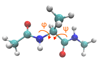
(a)  ALA-2 peptide with indicated dihedral angels.

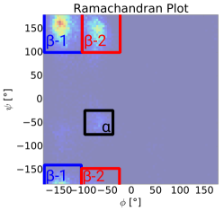
(b)  Characteristic conformations and their labelling as used in the sequel.

Figure 2: Definition of the dihedral angles and the labelling of characteristic modes as utilized in this paper.

The procedure for generating the training data for ALA-2 is similar to that in [Carmichael and Shell, 2012]. The atoms of the alanine dipeptide interact via the AMBER ff96 Sorin and Pande (2005); DePaul et al. (2010); Allen and Tildesley (1989) force field and we employ an implicit water model based on generalized Born/solvent accessible surface area model Onufriev, Bashford, and Case (2004); Still et al. (1990). However, we note that an explicit water model would better represent an experimental environment. We employ an Andersen thermostat and the simulations were carried out at constant temperature $T=$330\text{\,}\mathrm{K}$$ using Gromacs Berendsen, van der Spoel, and van Drunen (1995); Lindahl, Hess, and van der Spoel (2001); Spoel et al. (2005); Hess et al. (2008); Pronk et al. (2013); Páll et al. (2015); Abraham et al. (2015). The time step is taken as $\Delta t=$1\text{\,}\mathrm{f}\mathrm{s}$$ with an equilibration phase of $50\text{\,}\mathrm{n}\mathrm{s}$. The training dataset consisted of snapshots taken every $10\text{\,}\mathrm{p}\mathrm{s}$ after the equilibration phase. Rigid-body motions have been removed from the dataset.

For demonstrating the encoding into the latent CV space of atomistic configurations not contained in the training dataset, we used a test dataset selected so that the dihedral angles $(\phi,\psi)$ had values belonging to all three modes i.e. $\alpha$, $\beta\textnormal{-}1$, and $\beta\textnormal{-}2$ (defined in Fig. 2(b)).

III.1.2 Model specification

The model requires the specification of three components. Two components are needed to describe the generative model $p(\bm{x}|\bm{\theta})$: the probabilistic mapping $p_{\bm{\theta}}(\bm{x}|\bm{z})$ and the distribution of the CVs $p_{\bm{\theta}}(\bm{z})$. The third component is the approximate posterior $q_{\bm{\phi}}(\bm{z}|\bm{x})$ of the latent CVs as shown in Eq. (II.3).

Following [Kingma and Welling, 2013], the distribution of the CVs is taken to be a standard Gaussian,

$$p_{\bm{\theta}}(\bm{z})=p(\bm{z})=\mathcal{N}(\bm{z};\bm{0},\bm{I}).$$ (27)

The simplicity in the distribution in Eq. (27) is compensated by a flexible mapping from $\bm{z}$ to the atomistic coordinates $\bm{x}$. This probabilistic mapping (decoder) is given by a parametrized Gaussian as follows,

$$p_{\bm{\theta}}(\bm{x}|\bm{z})=\mathcal{N}(\bm{x};\bm{\mu}_{\bm{\theta}}(\bm{z}),\bm{S}_{\bm{\theta}}),$$ (28)

where,

$$\bm{\mu}_{\bm{\theta}}(\bm{z})=f_{\bm{\theta}}^{\bm{\mu}}(\bm{z}),$$ (29)

is a non-linear mapping $\bm{z}\mapsto f_{\bm{\theta}}^{\bm{\mu}}(\bm{z})$ ($f_{\bm{\theta}}^{\bm{\mu}}:\mathbb{R}^{n_{\text{CV}}}\mapsto\mathbb{R}^{n_{f}}$) parametrized by an expressive multilayer perceptron Rumelhart, Hinton, and Williams (1986); Van Der Malsburg (1986); Haykin (1998).

We consider a diagonal covariance matrix i.e. $\bm{S}_{\bm{\theta}}=\mathrm{diag}(\bm{\sigma}^{2}_{\bm{\theta}})$ Mattei and Frellsen (2018) where its entries $\sigma_{\bm{\theta},j}^{2}$ are treated as model parameters and do not depend on the latent CVs $\bm{z}$. In order to ensure the non-negativity of $\sigma^{2}_{\bm{\theta},j}>0$ while performing unconstrained optimization, we operate instead on $\log\sigma^{2}_{\bm{\theta},j}$.

The approximate posterior $q_{\bm{\phi}}(\bm{z}^{(i)}|\bm{x}^{(i)})$ of the latent variables (encoder, approximating $p_{\bm{\theta}}(\bm{z}^{(i)}|\bm{x}^{(i)})$) introduced in Eq. (II.3) is modeled by a Gaussian with flexible mean and variance represented by a neural network. For each pair of $\bm{x}^{(i)},\bm{z}^{(i)}$ (for notational simplicity, we drop the index $(i)$):

$$q_{\bm{\phi}}(\bm{z}|\bm{x})=\mathcal{N}(\bm{z};\bm{\mu}_{\bm{\phi}}(\bm{x}),\bm{S}_{\bm{\phi}}(\bm{x}))$$ (30)

where the covariance matrix is assumed to be diagonal i.e. $\bm{S}_{\bm{\phi}}(\bm{x})=\mathrm{diag}\left(\bm{\sigma}_{\bm{\phi}}^{2}(\bm{x})\right)$. Furthermore $\bm{\mu}_{\bm{\phi}}(\bm{x})$ and $\log\bm{\sigma}_{\bm{\phi}}^{2}(\bm{x})$ are taken as the outputs of the encoding neural networks $f^{\bm{\mu}}_{\bm{\phi}}(\bm{x})$ and $f^{\bm{\sigma}}_{\bm{\phi}}(\bm{x})$, respectively:

$$\bm{\mu}_{\bm{\phi}}(\bm{x})=f_{\bm{\phi}}^{\bm{\mu}}(\bm{x})\quad\text{and}\quad\log\bm{\sigma}_{\bm{\phi}}^{2}(\bm{x})=f_{\bm{\phi}}^{\bm{\sigma}}(\bm{x}).$$ (31)

We provide further details later in this section along with the structure of the employed networks. In our model, we assume a diagonal Gaussian approximation for $q_{\bm{\phi}}(\bm{z}|\bm{x})$.

We are aware that the actual, but intractable, posterior $p_{\bm{\theta}}(\bm{z}|\bm{x})$ could differ from a diagonal Gaussian and even from a multivariate normal distribution. However, the low variance $\bm{\sigma}_{\bm{\phi}}^{2}$ observed in test cases justifies the assumption of a diagonal Gaussian in this context. An enriched model for the approximate posterior $q_{\bm{\phi}}(\bm{z}|\bm{x})$ over the CVs could rely on e.g. normalizing flows Rezende and Mohamed (2015). Recent developments on autoregressive flows Kingma et al. (2016) overcome the practical restriction of normalizing flows to low-dimensional latent spaces. This discussion equally holds for the assumption of a Gaussian with diagonal covariance matrix for the generative distribution $p_{\bm{\theta}}(\bm{x}|\bm{z})$. In the latter case, the diagonal entries of the covariance matrix $\bm{S}_{\bm{\theta}}=\mathrm{diag}(\bm{\sigma}_{\bm{\theta}}^{2})$ were modeled as parameters independent of $\bm{z}$. Either using $\bm{S}_{\bm{\theta}}=\mathrm{diag}(\bm{\sigma}_{\bm{\theta}}^{2})$ or introducing a dependency on the latent CVs, $\bm{S}_{\bm{\theta}}(\bm{z})=\mathrm{diag}(\bm{\sigma}_{\bm{\theta}}^{2}(\bm{z}))$ does not influence the predictive quality in terms of observables and predicted atomistic configurations. This statement is particularly valid when an expressive model for the mean $\bm{\mu}_{\bm{\theta}}(\bm{z})$ in $p_{\bm{\theta}}(\bm{x}|\bm{z})$ (as in this work) is considered. It would be of interest employing more complex noise models for $p_{\bm{\theta}}(\bm{x}|\bm{z})$ which e.g. could be achieved by a Cholesky parametrization Pinheiro and Bates (1996). This might reveal structure correlations while reducing the need for higher complexity in $\bm{\mu}_{\bm{\theta}}(\bm{z})$.

As noted in Eq. (17), we employ the reparametrization trick by writing each random variable $\bm{z}^{(i,l)}\sim q_{\bm{\phi}}(\bm{z}^{(i)}|\bm{x}^{(i)})$ as

$$\bm{z}^{(i,l)}=g_{\bm{\phi}}(\bm{\epsilon}^{(l)};\bm{x}^{(i)})=\bm{\mu}_{\bm{\phi}}(\bm{x}^{(i)})+\bm{\sigma}_{\bm{\phi}}(\bm{x}^{(i)})\odot\bm{\epsilon}^{(l)},$$ (32)

and

$$\bm{\epsilon}^{(l)}\sim p(\bm{\epsilon})=\mathcal{N}(\bm{0},\bm{I}),$$ (33)

where $\odot$ denotes element-wise vector product.

We utilize the following structure for the decoding neural network $f_{\bm{\theta}}^{\bm{\mu}}(\bm{z})$:

$$f_{\bm{\theta}}^{\bm{\mu}}(\bm{z})=\left(l_{\bm{\theta}}^{(4)}\circ\tilde{a}^{(3)}\circ l_{\bm{\theta}}^{(3)}\circ\tilde{a}^{(2)}\circ l_{\bm{\theta}}^{(2)}\circ\tilde{a}^{(1)}\circ l_{\bm{\theta}}^{(1)}\right)(\bm{z}).$$ (34)

The encoding networks for obtaining $\bm{\mu}_{\bm{\phi}}(\bm{x})$ and $\bm{\sigma}^{2}_{\bm{\phi}}(\bm{x})$ of the approximate posterior $q_{\bm{\theta}}(\bm{z}|\bm{x})$ over the latent CVs share the structure,

$$f_{\bm{\phi}}(\bm{x})=\left(a^{(3)}\circ l_{\bm{\phi}}^{(3)}\circ a^{(2)}\circ l_{\bm{\phi}}^{(2)}\circ a^{(1)}\circ l_{\bm{\phi}}^{(1)}\right)(\bm{x}),$$ (35)

which gives rise to $f^{\bm{\mu}}_{\bm{\phi}}(\bm{x})$ and $f^{\bm{\sigma}}_{\bm{\phi}}(\bm{x})$ with,

$$f^{\bm{\mu}}_{\bm{\phi}}(\bm{x})=l_{\bm{\phi}}^{(4)}\left(f_{\bm{\phi}}(\bm{x})\right)\quad\text{and}\quad f^{\bm{\sigma}}_{\bm{\phi}}(\bm{x})=l_{\bm{\phi}}^{(5)}\left(f_{\bm{\phi}}(\bm{x})\right).$$ (36)

In Eqs. (34)-(36), we consider linear layers $l^{(i)}$ of a variable $\bm{y}$ with $l^{(i)}(\bm{y})=\bm{W}^{(i)}\bm{y}+\bm{b}^{(i)}$ and non-linear activation functions denoted with $a(\cdot)$. The indices $\bm{\phi}$ and $\bm{\theta}$ of the linear layers $l^{(i)}$ reflect correspondence to either the encoding or decoding network, respectively. $\bm{\phi}$ comprises all parameters of the encoding networks $f_{\bm{\phi}}^{\bm{\mu}}(\bm{x})$ and $f_{\bm{\phi}}^{\bm{\sigma}}(\bm{x})$, $\bm{\theta}$ all parameters of the decoding network $f_{\bm{\theta}}(\bm{z})$ including the parameters $\bm{\sigma}^{2}_{\bm{\theta}}$ discussed in Eq. (28). We differentiate the encoding and decoding activation functions by denoting them as $a^{(i)}$ and $\tilde{a}^{(i)}$, respectively. All layers considered were fully connected. The general architecture of the neural networks employed and how these affect the objective $\mathcal{L}(\bm{\theta},\bm{\phi};\bm{X})$ are depicted in Fig. 3.

Figure 3: Schematic of the AEVB depicting the employed network architecture. Fully connected linear layers are denoted with $l^{(i)}$ and non-linear activation functions with $a^{(i)}$. The indices $\bm{\phi}$ and $\bm{\theta}$ indicate encoding and decoding networks, respectively. The maximization of the lower-bound on the marginal log-likelihood $\mathcal{L}(\bm{\theta},\bm{\phi};\bm{X})$ in Eq. (11) simultaneously optimizes the parametrization of the encoder and decoder. The first term in $\mathcal{L}(\bm{\theta},\bm{\phi};\bm{X})$ accounts for the reconstruction of the training data $\bm{x}^{(i)}$ with $\bm{z}^{(i)}$ distributed according $q_{\bm{\phi}}(\bm{z}^{(i)}|\bm{x}^{(i)})$. The second term, in aggregation of all data $\bm{x}^{(i)}$, ensures that $q_{\bm{\phi}}(\bm{z}^{(i)}|\bm{x}^{(i)})$ is close to $p(\bm{z})$.

The optimization of the objective is carried out by a stochastic gradient ascent algorithm. In our case, we employ ADAM Kingma and Ba (2014) with the parameters chosen as $\alpha=0.001,\beta_{1}=0.9,\beta_{2}=0.999,\epsilon_{\text{ADAM}}=$1.0\text{\times}{10}^{-8}$$. Gradients of the lower-bound $\mathcal{L}(\bm{\theta},\bm{\phi};\bm{X})$ with respect to the model parametrization $\{\bm{\phi},\bm{\theta}\}$ are estimated by the backpropagation procedure Rumelhart, Hinton, and Williams (1986). The required gradients for optimizing the parameters $\bm{\sigma}^{2}_{\bm{\theta}}$ can be computed analytically. For an entry $\sigma_{j,\bm{\theta}}^{2}$, we can write the following:

$$\frac{\partial\mathcal{L}(\bm{\theta},\bm{\phi};\bm{x}^{(i)})}{\partial\log\sigma_{j,\bm{\theta}}^{2}} =\frac{\partial\log p_{\bm{\theta}}(\bm{x}^{(i)}|\bm{z})}{\partial\log\sigma_{j,\bm{\theta}}^{2}}$$

$$=\frac{\partial}{\partial\log\sigma_{j,\bm{\theta}}^{2}}\left(-\frac{1}{2}\sum_{j=1}^{\dim(\bm{x}^{(i)})}\frac{\left(x^{(i)}_{j}-\mu_{j,\bm{\theta}}(\bm{z})\right)^{2}}{\sigma_{j,\bm{\theta}}^{2}}\right)$$

$$=\frac{\partial}{\partial\log\sigma_{j,\bm{\theta}}^{2}}\left(-\frac{1}{2}\sum_{j=1}^{\dim(\bm{x}^{(i)})}\frac{\left(x^{(i)}_{j}-\mu_{j,\bm{\theta}}(\bm{z})\right)^{2}}{\exp\left(\log\left(\sigma_{j,\bm{\theta}}^{2}\right)\right)}\right)$$

$$=\frac{1}{2}\frac{\left(x^{(i)}_{j}-\mu_{j,\bm{\theta}}(\bm{z})\right)^{2}}{\sigma_{j,\bm{\theta}}^{2}}.$$ (37)

Linear layer	Input dimension	Output dimension	Activation layer	Activation function
$l_{\bm{\phi}}^{(1)}$	$\dim(\bm{x})$	$d_{1}$	$a^{(1)}$	SeLu
$l_{\bm{\phi}}^{(2)}$	$d_{1}$	$d_{2}$	$a^{(2)}$	SeLu
$l_{\bm{\phi}}^{(3)}$	$d_{2}$	$d_{3}$	$a^{(3)}$	Log Sigmoid
$l_{\bm{\phi}}^{(4)}$	$d_{3}$	$\dim(\bm{z})$	None	-
$l_{\bm{\phi}}^{(5)}$	$d_{3}$	$\dim(\bm{z})$	None	-

Table 1: Network specification of the encoding neural network with $d_{1}=50$, $d_{2}=100$, and $d_{3}=100$.

Linear layer	Input dimension	Output dimension	Activation layer	Activation function
$l_{\bm{\theta}}^{(1)}$	$\dim(\bm{z})$	$d_{3}$	$\tilde{a}^{(1)}$	Tanh
$l_{\bm{\theta}}^{(2)}$	$d_{3}$	$d_{2}$	$\tilde{a}^{(2)}$	Tanh
$l_{\bm{\theta}}^{(3)}$	$d_{2}$	$d_{1}$	$\tilde{a}^{(3)}$	Tanh
$l_{\bm{\theta}}^{(4)}$	$d_{1}$	$\dim(\bm{x})$	None	-

Table 2: Network specification of the decoding neural network with $d_{\{1,2,3\}}$ as defined in Table 1.

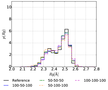
(a)  Varying dimensionality of the layers $l^{(i)}_{\{\bm{\theta},\bm{\phi}\}}$. The figure’s labels represent the dimensionality of the layers in the format $d_{1}$-$d_{2}$-$d_{3}$ as specified in Tables 1 and 2. We use the activation functions as denoted in the tables.

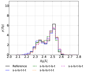
(b)  Testing different activation functions for $a^{(i)}$. The labels specify the utilized activation functions in the following manner: $a^{(1)}$-$a^{(2)}$-$a^{(3)}$-$\tilde{a}^{(1)}$-$\tilde{a}^{(2)}$-$\tilde{a}^{(3)}$. We use the abbreviations: t: Tanh, s: SeLu, ls: Log Sigmoid.

Figure 4: Prediction of the radius of gyration with differing networks, in terms of (a) the dimensionality of the layers and (b) regarding the type of activation functions used. Changes in the network specification lead to similar predictions. This model has been trained with a dataset of size $N=500$.

Studying different combinations of activation functions and layers for the encoding network $f^{\bm{\mu},\bm{\sigma}}_{\bm{\phi}}(\bm{x})$ and decoding network $f_{\bm{\theta}}^{\bm{\mu}}(\bm{z})$ led to the network architecture depicted in Tables 1 and 2, respectively. This network provided a repeatedly stable optimization during training. Variations of the given network architecture resulted into similar predictive capabilities as shown in Fig. 4. Stability is not limited to symmetric encoding and decoding activation functions. An automated approach for selecting or learning the best architecture is an active research area Ramachandran, Zoph, and Le (2017). Increasing the dimension of $\bm{z}$ did not improve the predictive capabilities as shown in Fig. 5. This implies that CVs with $\dim(\bm{z})=2$ suffice to capture the physics encapsulated in the ALA-2 dataset with $\dim(\bm{x})=66$ or $60$ DOF.

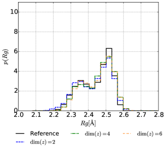
Figure 5: Predicted radius of gyration for models utilizing different $\dim(\bm{z})$. The predictions are based on a model as specified in Tables 1 and 2 with $N=500$.

III.1.3 Results

In the following illustrations, we trained the model by varying the number of snapshots $N$. We utilized a sub-sampled batch of size $M=64$ from the dataset of size $N$. In cases where $N<64$, we set $M=N$. The hyper parameters of the ARD prior in Eq. (20) are set to $a_{0}=b_{0}=$1.0\text{\times}{10}^{-5}$$. Other values for $a_{0},b_{0}$ in the range of $[$1.0\text{\times}{10}^{-8}$,$1.0\text{\times}{10}^{-4}$]$ were also employed without a significant effect on the obtained sparsity patterns or the predictive accuracy of the model.

Figure 6 depicts the $\bm{z}$-coordinates of $N=500$ training data as well as those of $1527$ test data which have been classified into the three modes based on the values of the dihedral angles (see Fig. 2(b)). In order to obtain the $\bm{z}$-coordinates of the test data, we made use of the mean $\bm{\mu}_{\bm{\phi}}(\bm{x}^{(i)})$ of the inferred approximate posterior $q_{\bm{\phi}}$ as obtained after training. The resulting picture essentially provides the pre-images of the atomistic configurations in the CV space. Interestingly, similar atomistic configurations, i.e. belonging to one of the three modes, $\alpha,\beta\textnormal{-}1,\beta\textnormal{-}2$, are recognized by $q_{\bm{\phi}}(\bm{z}|\bm{x})$ and mapped to clusters in the identified CV space. $\beta\textnormal{-}1$ configurations are encoded by $q_{\bm{\phi}}(\bm{z}|\bm{x})$ to regions with high probability mass in $p_{\bm{\theta}}(\bm{z})$, i.e. CVs $\bm{z}$ close to the center of $p_{\bm{\theta}}(\bm{z})=N(\bm{0},\bm{I})$ are assigned. This is in accordance with the reference Boltzmann distribution $p(\bm{x})$ where $\beta\textnormal{-}1$ is the most probable conformation.

Various dimensionality reduction methods are designed in order to keep similar $\bm{x}$ close in their embedding on the lower-dimensional CV manifold, e.g., multidimensional scaling Troyer and Cohen (1995) or ISOMAP Tenenbaum, Silva, and Langford (2000). In the presented scheme, the generative model learns that mapping similar $\bm{x}$ to similar $\bm{z}$ leads to an expressive (in terms of the marginal likelihood) lower-dimensional representation. This similarity is revealed by inferring the approximate latent variable posterior $q_{\bm{\phi}}(\bm{z}|\bm{x})$. Therefore, the desired similarity mentioned in [Rohrdanz, Zheng, and Clementi, 2013] between configurations in the atomistic representation $\bm{x}$ and via $q_{\bm{\phi}}(\bm{z}|\bm{x})$ in the assigned CVs $\bm{z}$ is achieved.

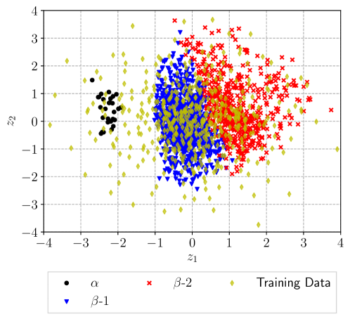
Figure 6: Representation of the $\bm{z}$-coordinates of the training data $\bm{X}$ with $N=500$ in the CV space (yellow diamonds). Using the trained model and the mean of $q_{\bm{\phi}}(\bm{z}|\bm{z})$ we computed the $\bm{z}$-coordinates of $1527$ test samples corresponding to different conformations of the alanine dipeptide to $\alpha$ (black), $\beta\textnormal{-}1$ (blue), and $\beta\textnormal{-}2$ (red). Without any prior physical information, the encoder yields three distinct clusters in the CV space.

In contrast to several other dimensionality reduction techniques (e.g. Isomap Tenenbaum, Silva, and Langford (2000) and Diffusion maps Coifman et al. (2005a, b); Nadler et al. (2006); Ferguson et al. (2011b)), which as mentioned in the introduction require large amounts of training data e.g. $N>$10\,000$$ Rohrdanz, Zheng, and Clementi (2013); Duan et al. (2013), the proposed method can perform well in the small data regime, e.g. for $N=50$ as shown in  Fig. 7. The latter depicts the Ramachandran plot in terms of the dihedral angles based on various amounts of training data $N$ and compares it with the one predicted by the trained model on the same $N$ as well as with the reference (obtained with $N=$10\,000$$). We note that the trained model yields Ramachandran plots that more closely resemble the reference as compared to the ones computed by the training data alone. The encoder, trained with $N=200$, is capable of generating atomistic configurations leading to $(\phi,\psi)$ tuples which are not included in the training data.

The ARD prior in Eq. (20) drives $58$% of the parameters $\bm{\theta}$ to zero (as a threshold, we consider a parameter to be inactive when its value drops below $1.0\text{\times}{10}^{-4}$). In contrast, all network parameters $\bm{\theta}$ remain active while optimizing the objective without the ARD prior. Apart from the qualitative advantage, the sparsity-inducing prior provides a strong regularization in the presence of limited data and yields superior predictive estimates. In addition to obtaining sparse solutions, the ARD prior facilitates the identification of physically meaningful latent representations for limited data (e.g. $N=50$) as shown in Fig. 8. Without the ARD prior, the data is encoded in a rather small region of the latent space.

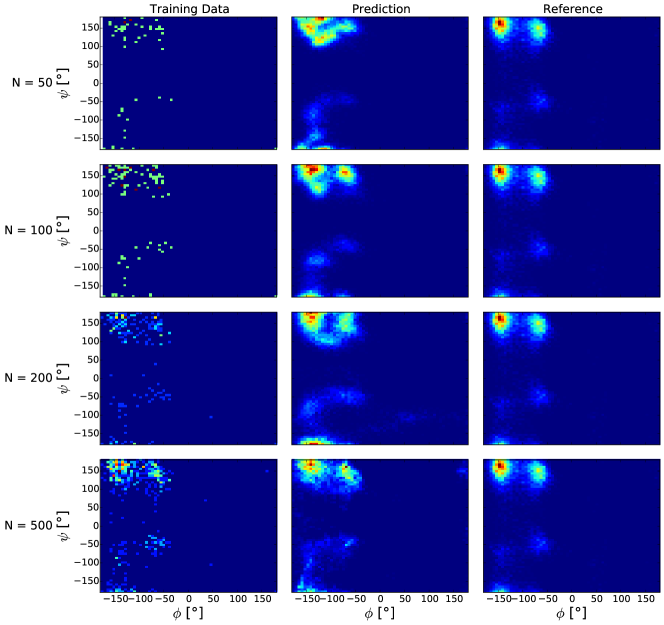
Figure 7: Ramachandran plots estimated with the training data $\bm{X}$ (left column), using predictions of the trained model (middle column), and the reference (right column, estimated with $N=$10\,000$$). Each row refers to different size $N$ of training datasets (the figure on the right column is repeated to allow easy comparison with the results on the first two columns). The represented predictions are obtained by applying Algorithm 2 with $T=$10\,000$$ samples. The generative nature of the model allows more accurate estimates than when using the training data alone. In addition, the Bayesian approach allows for predictions with their associated uncertainties as discussed subsequently.

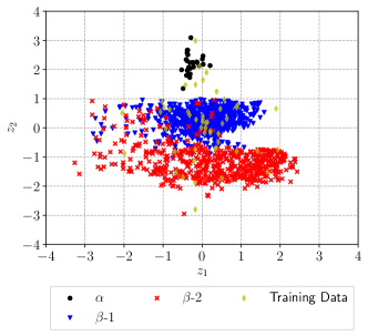
(a)  Active ARD prior.

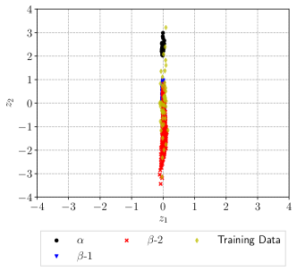
(b)  Without ARD prior.

Figure 8: Representation of the $\bm{z}$-coordinates of the training data $\bm{X}$ with $N=50$ in the CV space (yellow diamonds). Using the trained model and the mean of $q_{\bm{\phi}}(\bm{z}|\bm{z})$ we computed the $\bm{z}$-coordinates of $1527$ test samples corresponding to different conformations of the alanine dipeptide to $\alpha$ (black), $\beta\textnormal{-}1$ (blue), and $\beta\textnormal{-}2$ (red). In the case of limited training data, the ARD prior facilitates the identification of physically meaningful CVs (left) compared to the representation on the right obtained without the ARD prior. Note that the changed positioning of the conformations in the CV space compared to Fig. 6 is due to symmetries in $p_{\bm{\theta}}(\bm{z})$.

In Fig. 9, we attempt to provide insight on the physical meaning of the CVs $\bm{z}$ identified. In particular, we plot the atomistic configurations $\bm{x}$ corresponding to various values of the first CV $z_{1}$ while keeping $z_{2}=0$. The conformational transition in predicted atomistic configurations can be clearly recognized in the peptides of Fig. 9. We note that we start on the left ($z_{1}<0$) with $\alpha$ configurations, then move towards $\beta\textnormal{-}1$ (starting at $z_{1}\approx-1$), and finally obtain $\beta\textnormal{-}2$ configurations. For illustration purposes, the predictions in  Fig. 9 are based solely on the mean $\bm{\mu}_{\bm{\theta}}(\bm{z})$ of the probabilistic decoder $p_{\bm{\theta}}(\bm{x}|\bm{z})=\mathcal{N}(\bm{x};\bm{\mu}_{\bm{\theta}}(\bm{z}),\bm{S}_{\bm{\theta}}=\mathrm{diag}(\bm{\sigma}_{\bm{\theta}}^{2}))$. We note that for each value of the CVs $\bm{z}$ several atomistic realizations $\bm{x}$ can be drawn from $p_{\bm{\theta}}(\bm{x}|\bm{z})$ as depicted in Fig. 10. This figure reveals the characteristic and relevant movement of the backbone that is captured by the predictive mean $\bm{\mu}_{\bm{\theta}}(\bm{z})=f^{\bm{\mu}}_{\bm{\theta}}(\bm{z})$. Fluctuations of less relevant outer Hydrogen atoms (see Figs. 10(b)-10(d)) are recognized as noise of the decoder $p_{\bm{\theta}}(\bm{x}|\bm{z})=\mathcal{N}\left(\bm{\mu}(\bm{z}),\bm{S}_{\bm{\theta}}=\mathrm{diag}(\bm{\sigma}_{\bm{\theta}}^{2})\right)$ denoted in Eq. (28). We note also that the corresponding entries of $\bm{\sigma}_{\bm{\theta}}$ responsible for the outer Hydrogen atoms are five times larger compared to the remaining atoms. The proposed model can therefore in unsupervised fashion identify the central role of the backbone coordinates whereas this physical insight is pre-assumed in [Wehmeyer and Noé, 2018; Chen and Ferguson, 2018].

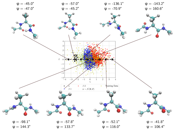
Figure 9: Predicted configurations $\bm{x}$ (including dihedral angle values) for $\{\bm{z}|z_{1}=\{-3.5,-2.5,\dots,3.5\},z_{2}=0\}$ with $\bm{\mu}_{\bm{\theta}}(\bm{z})$ of $p_{\bm{\theta}}(\bm{x}|\bm{z})$. As one moves along the $z_{1}$ axis, we obtain for the given CVs atomistic configurations $\bm{x}$ reflecting the conformations $\alpha$, $\beta\textnormal{-}1$, and $\beta\textnormal{-}2$. All rendered atomistic representations in this work are created by VMD Humphrey, Dalke, and Schulten (1996).

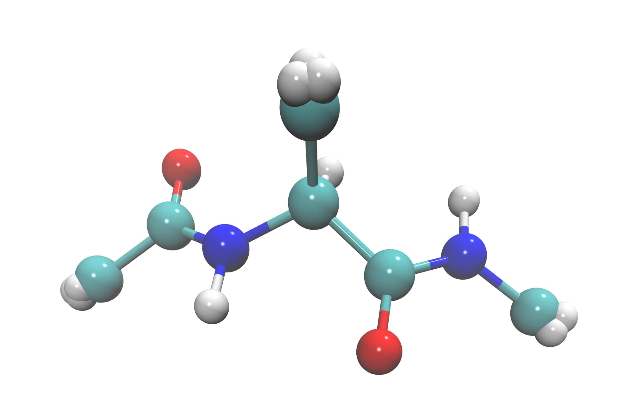
(a)  Mean prediction $\bm{\mu}_{\bm{\theta}}(\bm{z}^{0})$ for a sample $\bm{z}^{0}\sim p(\bm{z})$.

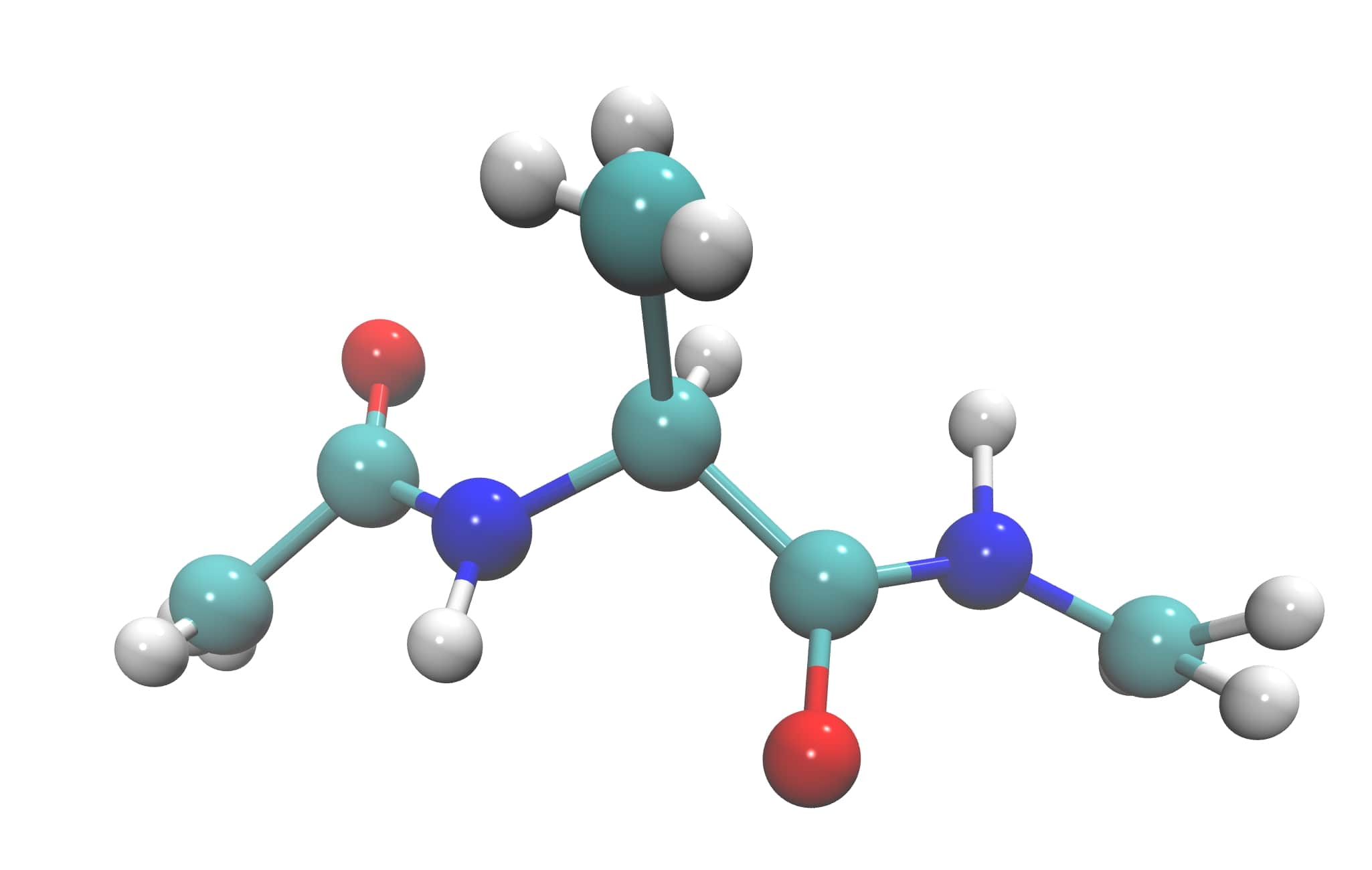
(b)  Realization $\bm{x}^{0,0}\sim p_{\bm{\theta}}(\bm{x}|\bm{\mu}_{\bm{\theta}}(\bm{z}^{0}),\bm{S}_{\bm{\theta}}=\mathrm{diag}(\bm{\sigma}_{\bm{\theta}}^{2}))$.

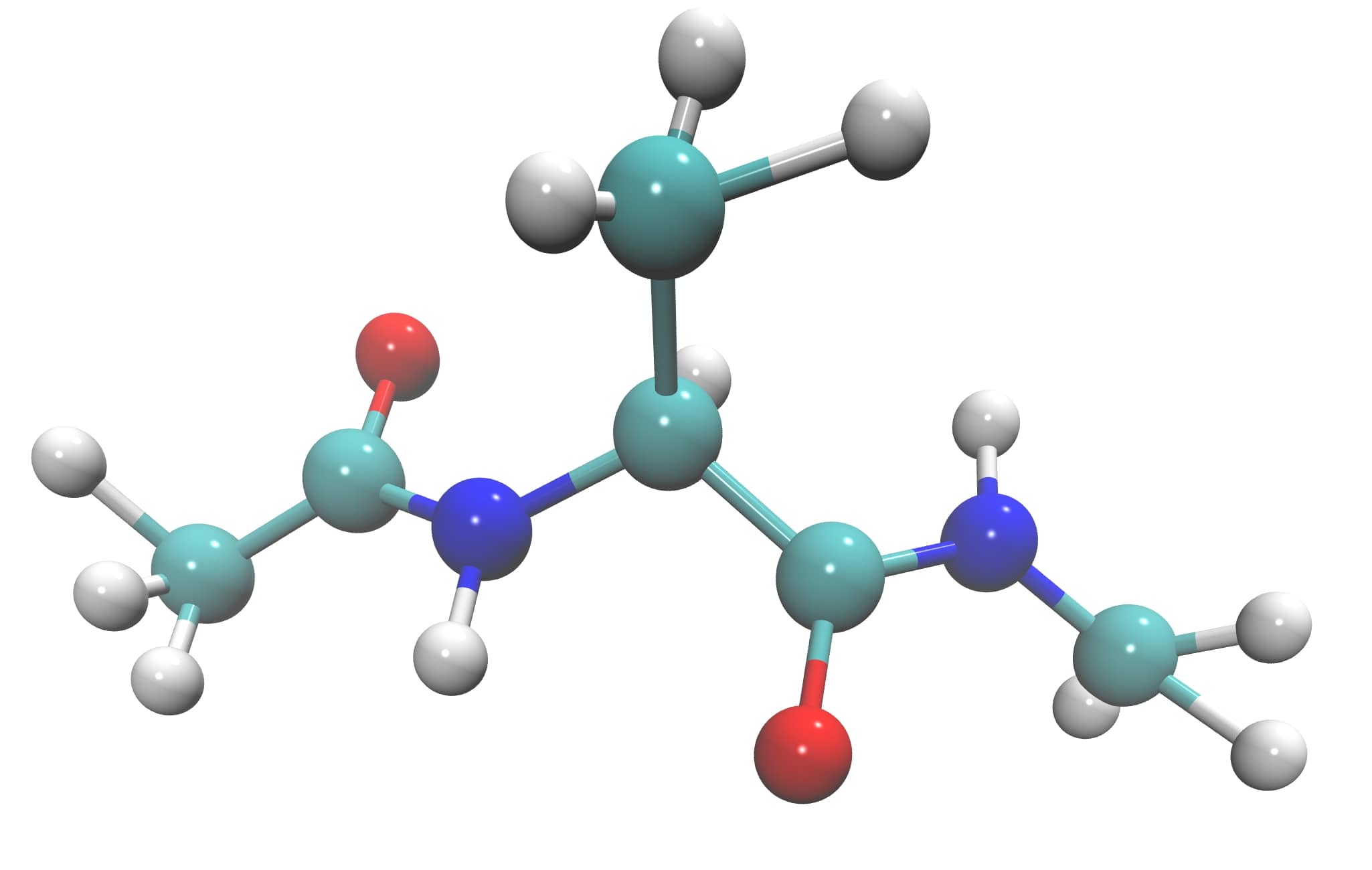
(c)  Realization $\bm{x}^{1,0}\sim p_{\bm{\theta}}(\bm{x}|\bm{\mu}_{\bm{\theta}}(\bm{z}^{0}),\bm{S}_{\bm{\theta}}=\mathrm{diag}(\bm{\sigma}_{\bm{\theta}}^{2}))$.

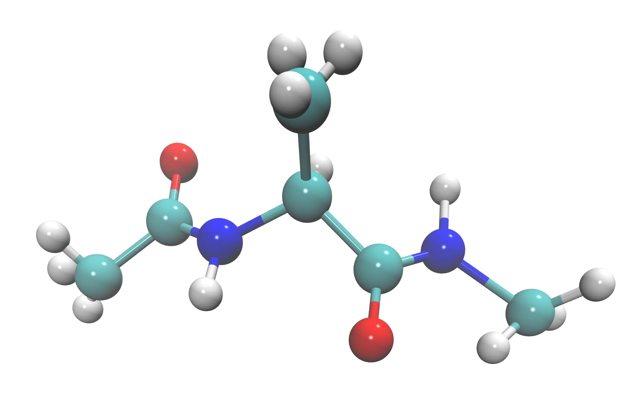
(d)  Realization $\bm{x}^{2,0}\sim p_{\bm{\theta}}(\bm{x}|\bm{\mu}_{\bm{\theta}}(\bm{z}^{0}),\bm{S}_{\bm{\theta}}=\mathrm{diag}(\bm{\sigma}_{\bm{\theta}}^{2}))$.

Figure 10: Visualization of the mean prediction (a) for a sample $\bm{z}^{0}\sim p(\bm{z})$, obtained from the decoding network $\bm{\mu}_{\bm{\theta}}(\bm{z}^{0})=f_{\bm{\theta}}(\bm{z}^{0})$, and realizations (b-d) $\bm{x}^{j,0}\sim p_{\bm{\theta}}(\bm{x}|\bm{z}^{0})$. Less relevant positions of the outer Hydrogen atoms are captured by the noise $\bm{\sigma}_{\bm{\theta}}$ of the model $p_{\bm{\theta}}(\bm{x}|\bm{z}^{0})=\mathcal{N}(\bm{\mu}(\bm{z}_{\bm{\theta}}^{0}),\bm{S}_{\bm{\theta}}=\mathrm{diag}(\bm{\sigma}_{\bm{\theta}}^{2}))$.

In order to gain further insight into the relation between the dihedral angles $\phi,\psi$ and the discovered CVs $\bm{z}$, we plot in Figs. 11 and 12 the corresponding maps for various combinations of $\bm{z}$-values. While it is clear that the map is not always bijective, the figures reveal the strong correlation between the two sets of variables. It should also be noted that in contrast to the dihedral angles, the $\bm{z}$ value for a given atomistic configuration $\bm{x}$ are not unique but rather there is a whole distribution as implied by $q_{\bm{\phi}}(\bm{z}|\bm{x})$. For the aforementioned plots we computed the $\bm{z}$ from the mean of this density, i.e. $\bm{\mu}_{\bm{\phi}}(\bm{x})$.

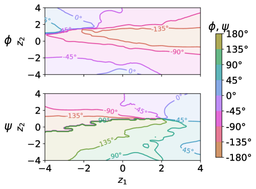
Figure 11: Predicted dihedral angles $(\phi,\psi)$ given the latent variables $\bm{z}\in[-4,4{]^{2}}$.

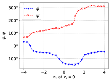
(a)  

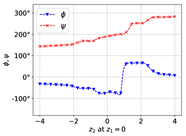
(b)  

Figure 12: Predicted dihedral angles $(\phi,\psi)$ given the latent variables (a) $\{z_{1},z_{2}|z_{1}\in[-4,4],z_{2}=0\}$ and (b) $\{z_{1},z_{2}|z_{1}=0,z_{2}\in[-4,4]\}$.

The trained model can also be employed in computing predictive estimates of observables $\int a(\bm{x})~{}p_{target}(\bm{x})~{}d\bm{x}$ by making use of $p_{\bm{\theta}}(\bm{x})$ and samples drawn from it as described in Section II.4. We illustrate this by computing the radius of gyration (Rg) Fluitt and de Pablo (2015); Carmichael and Shell (2012) given as,

$$a_{\text{Rg}}(\bm{x})=\sqrt{\frac{\sum_{p}m_{p}||\bm{x}_{p}-\bm{x}_{\text{COM}}||^{2}}{\sum_{p}m_{p}}}.$$ (38)

The sum in Eq. (38) considers all atoms $p=1,\ldots,P$ of the peptide, where $m_{p}$ and $\bm{x}_{p}$ denote the mass and the coordinates of each atom, respectively. $\bm{x}_{\text{COM}}$ denotes the center of mass of the peptide. The histogram of $a_{\text{Rg}}(\bm{x})$ reflects the distribution of the size of the peptide and is correlated with the various conformations Fluitt and de Pablo (2015).

In the estimates that we depict in Fig. 13, we have also employed the posterior approximation of the model parameters $\bm{\theta}$ obtained as described in Section II.6 in order to compute credible intervals for the observable. These credible intervals are estimated as described in Algorithm 4 utilizing $J=$3000$$ samples. We observe that the model’s predictive confidence increases with the size of the training data. This is reflected in shrinking credible intervals in Fig. 13 for increasing $N$.

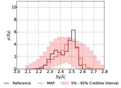
(a)  $N=50$.

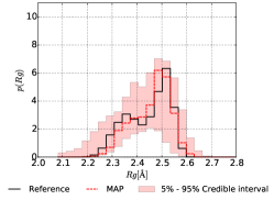
(b)  $N=200$.

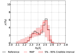
(c)  $N=500$.

Figure 13: Predicted radius of gyration with $\dim(\bm{z})=2$ for various sizes $N$ of the training dataset. The MAP estimate indicated in red is compared to the reference (black) solution. The latter is estimated by $N=$10\,000$$. The shaded area represents the 5%-95% credible interval, reflecting the induced epistemic uncertainty from the limited amount of training data.

Algorithm 4 Estimating Credible Intervals.

$J$ the number of samples to be drawn, optimal values of $\bm{\theta}=\bm{\theta}_{MAP}$ and $\bm{\phi}=\bm{\phi}_{MAP}$.

Compute Laplace’s approximation $\mathcal{N}(\bm{\mu}_{L},\bm{S}_{L}=\mathrm{diag}(\bm{\sigma}_{L}^{2}))$ to the posterior $p(\bm{\theta}|\bm{X})$ (Eq. (24)).

for $j=1$ to J  do

   Draw a posterior sample: $\bm{\theta}^{j}\sim\mathcal{N}(\bm{\mu}_{L},\bm{S}_{L}=\mathrm{diag}(\bm{\sigma}_{L}^{2}))$.

   Obtain a predictive trajectory $\bar{\bm{x}}_{1:T}^{j}$, given the parametrization $\bm{\theta}^{j}$ utilizing Algorithm 2.

   Estimate the observable $\hat{a}(\bm{\theta}^{j})=\frac{1}{T}\sum_{t=1}^{T}a(\bar{\bm{x}}^{j}_{t})$, given the trajectory $\bar{\bm{x}}_{1:T}^{j}$.

end for

Estimate the desired quantiles with $\hat{a}(\bm{\theta}^{1:J})$.

In summary for ALA-2, we note that the proposed methodology for identifying CVs (Fig. 6) and predicting observables (Figs. 7 and 13) works well with small size datasets, e.g. $N=\{50,200,500\}$.

III.2 ALA-15

III.2.1 Simulation of ALA-15 and model specification

The following example considers a larger alanine peptide with $15$ residues, ALA-15 which consists of $162$ atoms giving rise to $\dim(\bm{x})=486$ with $480$ DOF. The reference dataset $\bm{X}$ has been obtained in a similar manner as specified in Section III.1.1 with the only difference being that we utilize a replica-exchange molecular dynamics Sugita and Okamoto (1999) algorithm with $21$ temperature replicas distributed according to $T_{i}=T_{0}e^{\kappa\cdot i}$ ($T_{0}=$270\text{\,}\mathrm{K}$$, and $\kappa=0.04$). This leads to an analogous simulation setting as employed in [Carmichael and Shell, 2012]. The datasets are obtained as mentioned in the previous example. We consider here $N=\{300,$3000$,$5000$\}$. Using the same model specifications as in Section III.1.2, we present next a summary of the obtained results.

III.2.2 Results

For visualization purposes of the latent CV space, we assumed $\dim(\bm{z})=2$ in the following, even though the presence of 15 residues each requiring a pair of dihedral angles $(\phi,\psi)$ would potentially suggest a higher-dimensional representation. However, when considering test cases with $\dim(\bm{z})=\{15,30\}$, no significant differences were observed in the predictive capabilities. This is in agreement with [Marini and Dong, 2011] where it is argued based on density functional theory calculations that not all dihedral angles are equally relevant. The $(\phi,\psi)$ pairs within a peptide chain show high correlation. Mulitlayer neural networks provide the capability of transforming independent CVs (as considered in this study) to correlated ones by passing them through the subsequent network layers. This explains the reasonable predictive quality of the model using independent and low-dimensional CVs with $\dim(\bm{z})=2$. Considering more expressive $p_{\bm{\theta}}(\bm{z})$ than the standard Gaussian employed, could have accounted (in part) for such correlations. In this example, by employing the ARD prior, only $43$% of the decoder parameters $\bm{\theta}$ remained effective.

Figure 14 depicts the posterior means of the $N=$3000$$ training data in the CV space $\bm{z}$. Given that a peptide configuration contains residues from different conformations labelled here as $\alpha$, $\beta\textnormal{-}1$, and $\beta\textnormal{-}2$ and residues in intermediate $(\phi,\psi)$ states, we applied the following rule for labelling/coloring each datapoint. The assigned color in Fig. 14 is a mixture between the RGB colors black (for $\alpha$), blue (for $\beta\textnormal{-}1$), and red (for $\beta\textnormal{-}2$). The mixture weights of the assigned color are proportional to the number of residues belonging to the $\alpha$ (black), $\beta\textnormal{-}1$ (blue), and $\beta\textnormal{-}2$ (red) conformations, normalized by the total amount of residues which can be clearly assigned to $\alpha$, $\beta\textnormal{-}1$, and $\beta\textnormal{-}2$. Additionally, we visualize the amount of intermediate $(\phi,\psi)$ states of the residues by the opacity of the scatter points. The opacity reflects the amount of residues which are clearly assigned to the $\alpha$, $\beta\textnormal{-}1$, and $\beta\textnormal{-}2$ conformations compared to the total amount of residues in the peptide. For example, if all residues of a peptide configuration correspond to a specific mode, the opacity is taken as $100$%. If all residues are in non-classified intermediate states, the opacity is set to the minimal value which is here taken as $20$%.

We note that peptide configurations in which the majority of residues belong to $\beta\textnormal{-}1$ (blue) or in the $\beta\textnormal{-}2$ conformation (red), are clearly separated in the CV space from datapoints with residues predominantly in the $\alpha$ conformation (black). Nevertheless, we observe that the encoder has difficulties separating blue ($\beta\textnormal{-}1$) and red ($\beta\textnormal{-}2$) datapoints. We remark though that the related secondary structures Zhou et al. (2016) resulting from the assembly of residues in $\beta\textnormal{-}1$ and $\beta\textnormal{-}2$, such as the $\beta$-sheet and $\beta$-hairpin, share a similar atomistic representation $\bm{x}$ which explains the similarity in the CV space.

When one moves in the CV space $\bm{z}$ along the path indicated by a red dashed line in Fig. 15 and reconstructs the corresponding $\bm{x}$ using the mean function of the decoder $p_{\bm{\theta}}(\bm{x}|\bm{z})$, we obtain atomistic configurations of the ALA-15 partially consisting of the conformations $\alpha$, $\beta\textnormal{-}1$, and $\beta\textnormal{-}2$ which correspond to the aforementioned secondary structures i.e. $\beta$-sheet (top left), $\beta$-hairpin (top middle and right), and $\alpha$-helix (bottom row).

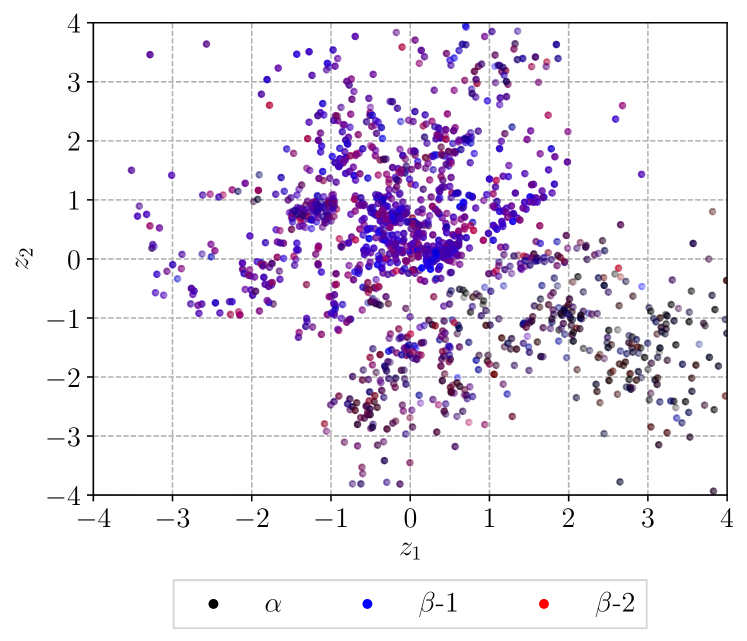
Figure 14: Representation of the training data $\bm{X}$ with $N=$3000$$ in the encoded collective variable space. The inferred approximate posterior $q_{\bm{\phi}}(\bm{z}|\bm{x})$ of the latent CVs separates residues mostly belonging to the $\beta$ conformations (mixture of red and blue) and peptide configurations containing largely residues in the $\alpha$ configuration (black). Here, the mean $\bm{\mu}_{\bm{\phi}}(\bm{x})$ of the approximate posterior $q_{\bm{\phi}}(\bm{z}|\bm{x})=\mathcal{N}(\bm{x};\bm{\mu}_{\bm{\phi}}(\bm{x}),\bm{S}_{\bm{\phi}}=\mathrm{diag}(\bm{\sigma}_{\bm{\phi}}^{2}(\bm{x})))$ is depicted.

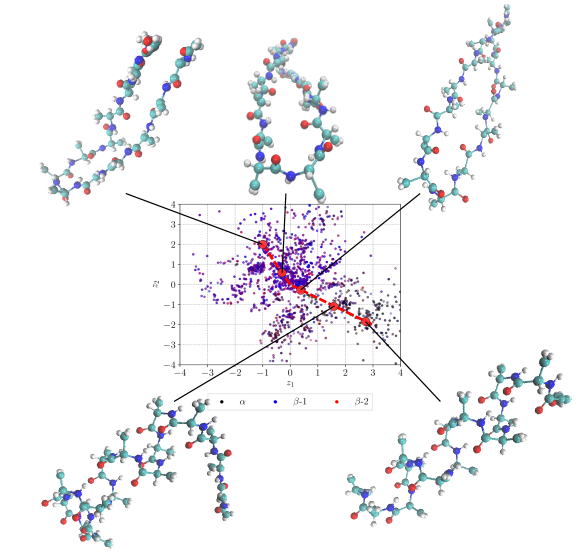
Figure 15: Predicted configurations $\bm{x}$ for decoding CVs indicated as red points on the dashed line in the plot. Depicted configurations have been produced by evaluating the mean $\bm{\mu}_{\bm{\theta}}(\bm{z})$ of $p_{\bm{\theta}}(\bm{x}|\bm{z})$. Moving along the path, we obtain atomistic configurations $\bm{x}$ partially consisting of the conformations $\alpha$, $\beta\textnormal{-}1$, and $\beta\textnormal{-}2$ in the ALA-15 peptide resulting into peptide secondary structures such as $\beta$-sheet (top left), $\beta$-hairpin (top middle and right), and $\alpha$-helix (bottom row).

The ambiguity between $\beta\textnormal{-}1$ and $\beta\textnormal{-}2$ states is also reflected in the predicted Ramachandran plot in Fig. 16.

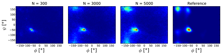
Figure 16: Predicted Ramachandran plots with $\dim(\bm{z})=2$ for various sizes $N$ of the training dataset (first three plots from the left). Depicted predictions are MAP estimates based on $T=$10\,000$$ samples. The plot on the right is the reference MD prediction with $N=$10\,000$$ configurations.

Nevertheless properties, independent of the explicit separation of configurations predominantly consisting of residues in $\beta\textnormal{-}1$ and $\beta\textnormal{-}2$ states, are predicted accurately by the framework. This is demonstrated with the computed radius of gyration in Fig. 17. The MAP estimate is complemented by the credible intervals which reflect the epistemic uncertainty and are able to envelop the reference profile. As in the previous example, the breadth of the credible intervals shrinks with increasing training data $N$.

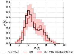
(a)  $N=300$.

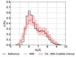
(b)  $N=$3000$$.

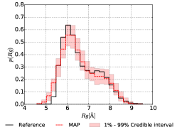
(c)  $N=$5000$$.

Figure 17: Predicted radius of gyration with $\dim(\bm{z})=2$ for various sizes $N$ of the training dataset. The MAP estimate indicated in red is compared to the reference (black) solution. The latter is estimated by $N=$10\,000$$. The shaded area represents the 1%-99% credible interval, reflecting the induced epistemic uncertainty from the limited amount of training data.

IV Conclusions

We presented an unsupervised learning scheme for discovering CVs of atomistic systems. We defined the CVs as latent generators of the atomistic configurations and formulated their identification as a Bayesian inference task. Inference of the posterior distribution of the latent CVs given the fine-scale atomistic training data identifies a probabilistic mapping from the space of atomistic configurations to the latent space. This posterior distribution resembles a dictionary translating atomistic configurations to the lower-dimensional CV space which is inferred during the training procedure. Compared to other dimensionality reduction methods, the proposed scheme is capable of performing well with comparably heterogeneous and small datasets.

We presented the capabilities of the model for the test case of an ALA-2 peptide (Section III). When the dimensionality of the CVs $\dim(\bm{z})$ was set to $2$, the model discovered variables that correlate strongly with the widely known dihedral angles $(\phi,\psi)$. Other dimensionality reduction methods Hotelling (1933); Troyer and Cohen (1995); Härdle and Simar (2007); Tenenbaum, Silva, and Langford (2000); Coifman et al. (2005a, b); Nadler et al. (2006) rely on an objective keeping small distances between configurations in the atomistic space also small in the latent space. Rather than enforcing this requirement directly, the proposed framework identifies a lower-dimensional representation that clusters configurations in the CV space which show similarities in the atomistic space. The Bayesian formulation presented allows for a rigorous quantification of the unavoidable uncertainties and their propagation in the predicted observables. The ARD prior chosen was shown to lead to on average $45\%$ less parameters compared to the optimization without it.

We presented an approach for approximating the intractable posterior of the decoding model parameters (Eq. (24)) and provided an algorithm (Algorithm 4) for estimating credible intervals. The uncertainty propagated to the observables captures the parameter uncertainty of the decoding neural network $f_{\bm{\theta}}^{\bm{\mu}}(\bm{z})$.

In addition to discovering CVs, the generative model employed is able to predict atomistic configurations by sampling the CV space with $p_{\bm{\theta}}(\bm{z})$ and mapping the CVs probabilistically via $p_{\bm{\theta}}(\bm{x}|\bm{z})$ to full atomistic configurations. We showed that the predictive mapping $p_{\bm{\theta}}(\bm{x}|\bm{z})$ recognizes essential backbone behavior of the peptide while it models fluctuations of the outer Hydrogen atoms with the noise of $p_{\bm{\theta}}(\bm{x}|\bm{z})$ (see Fig. 10). We use the model for predicting observables and quantifying the uncertainty arising from limited training data.

We emphasize that the whole work was based on data represented by Cartesian coordinates $\bm{x}$ of all the atoms of the ALA-2 ($\dim(\bm{x})=66$, and $60$ DOF adjusted by removing rigid-body motion) and ALA-15 ($\dim(\bm{x})=486$, and $480$ DOF adjusted by removing rigid-body motion) peptides. Considering a pre-processed dataset e.g. by considering solely coordinates of the backbone atoms, heavy atom positions, or a representation by dihedral angles assumes the availability of tremendous physical insight. The aim of this work was to reveal CVs with physicochemical meaning and the prediction of observables of complex systems without using any domain-specific physical notion.

Besides the framework proposed, generative adversarial networks (GANs) Goodfellow et al. (2014) and its Bayesian reformulation in [Saatci and Wilson, 2017] open an additional promising avenue in the context of CV discovery and enhanced sampling of atomistic systems. GANs are accompanied by a two player (generator and discriminator) min-max objective which poses known difficulties in training the model. The training of GANs is not as robust as the VAE employed here and Bayesian formulations are not well studied. In addition, one needs to address the mode collapse issue (see [Salimans et al., 2016]) which is critical for atomistic systems.

Future work involves the use of the CVs discovered in the context of enhanced sampling techniques that can lead to an accelerated exploration of the configurational space. In addition to identifying good CVs, a crucial step for enhanced sampling methods is the biasing potential for lifting deep free-energy wells. In contrast to the ideas e.g. presented in [Chen and Ferguson, 2018, Chen and Tuckerman, 2018, Galvelis and Sugita, 2017], we would advocate a formulation where the biasing potential is based on the lower-dimensional pre-image of the currently visited free-energy surface. To that end, we envision using the posterior distribution $q_{\bm{\phi}}(\bm{z}|\bm{x})$ to construct a locally optimal biasing potential defined in the CV space which gets updated on the fly as the simulations explore the configuration space. The biasing potential can be transformed by the probabilistic mapping of the generative model $p_{\bm{\theta}}(\bm{x}|\bm{z})$ to the atomistic description as follows,

$$U^{\bm{x}^{(i)}}_{\text{bias}}(\bm{x})\propto-\log\int_{\mathcal{M}_{CV}}p_{\bm{\theta}}(\bm{x}|\bm{z})q_{\bm{\phi}}(\bm{z}|\bm{x}^{(i)})~{}d\bm{z}.$$ (39)

Equation (39) is differentiable with respect to atomistic coordinates. Subtracting it from the atomistic potential could accelerate the simulation by “filling-in” the deep free-energy wells.

References

- Perilla et al. (2015) J. R. Perilla, B. C. Goh, C. K. Cassidy, B. Liu, R. C. Bernardi, T. Rudack, H. Yu, Z. Wu, and K. Schulten, Current Opinion in Structural Biology 31, 64 (2015).
- Koutsourelakis, Zabaras, and Girolami (2016) P. Koutsourelakis, N. Zabaras, and M. Girolami, Journal of Computational Physics 321, 1252 (2016).
- Barducci, Bonomi, and Parrinello (2011a) A. Barducci, M. Bonomi, and M. Parrinello, Wiley Interdisciplinary Reviews: Computational Molecular Science 1, 826 (2011a).
- Pietrucci and Andreoni (2011) F. Pietrucci and W. Andreoni, Phys. Rev. Lett. 107, 085504 (2011).
- Ferguson et al. (2011a) A. L. Ferguson, A. Z. Panagiotopoulos, P. G. Debenedetti, and I. G. Kevrekidis, The Journal of Chemical Physics 134, 135103 (2011a), https://doi.org/10.1063/1.3574394 .
- Zheng, Rohrdanz, and Clementi (2013) W. Zheng, M. A. Rohrdanz, and C. Clementi, The Journal of Physical Chemistry B 117, 12769 (2013), pMID: 23865517, https://doi.org/10.1021/jp401911h .
- Valsson and Parrinello (2014) O. Valsson and M. Parrinello, Phys. Rev. Lett. 113, 090601 (2014).
- Chen and Ferguson (2018) W. Chen and A. L. Ferguson, Journal of Computational Chemistry 39, 2079 (2018), https://onlinelibrary.wiley.com/doi/pdf/10.1002/jcc.25520 .
- Chen and Tuckerman (2018) P.-Y. Chen and M. E. Tuckerman, The Journal of Chemical Physics 148, 024106 (2018), https://doi.org/10.1063/1.4999447 .
- Mitsutake, Mori, and Okamoto (2013) A. Mitsutake, Y. Mori, and Y. Okamoto, “Enhanced sampling algorithms,” in Biomolecular Simulations: Methods and Protocols, edited by L. Monticelli and E. Salonen (Humana Press, Totowa, NJ, 2013) pp. 153–195.
- Bierig and Chernov (2016) C. Bierig and A. Chernov, Journal of Computational Physics 314, 661 (2016).
- Luque and Barril (2012) J. Luque and X. Barril, eds., Physico-Chemical and Computational Approaches to Drug Discovery, RSC Drug Discovery (The Royal Society of Chemistry, 2012) pp. FP001–418.
- Rohrdanz, Zheng, and Clementi (2013) M. A. Rohrdanz, W. Zheng, and C. Clementi, Annual Review of Physical Chemistry 64, 295 (2013), pMID: 23298245, https://doi.org/10.1146/annurev-physchem-040412-110006 .
- Torrie and Valleau (1977) G. Torrie and J. Valleau, Journal of Computational Physics 23, 187 (1977).
- Voter (1997) A. F. Voter, The Journal of Chemical Physics 106, 4665 (1997), https://doi.org/10.1063/1.473503 .
- Hamelberg, Mongan, and McCammon (2004) D. Hamelberg, J. Mongan, and J. A. McCammon, The Journal of Chemical Physics 120, 11919 (2004), https://doi.org/10.1063/1.1755656 .
- Huber, Torda, and van Gunsteren (1994) T. Huber, A. E. Torda, and W. F. van Gunsteren, Journal of Computer-Aided Molecular Design 8, 695 (1994).
- Grubmüller (1995) H. Grubmüller, Phys. Rev. E 52, 2893 (1995).
- Laio and Parrinello (2002) A. Laio and M. Parrinello, Proceedings of the National Academy of Sciences 99, 12562 (2002), http://www.pnas.org/content/99/20/12562.full.pdf .
- Barducci, Bonomi, and Parrinello (2011b) A. Barducci, M. Bonomi, and M. Parrinello, Wiley Interdisciplinary Reviews: Computational Molecular Science 1, 826 (2011b), https://onlinelibrary.wiley.com/doi/pdf/10.1002/wcms.31 .
- Darve, Rodríguez-Gómez, and Pohorille (2008) E. Darve, D. Rodríguez-Gómez, and A. Pohorille, The Journal of Chemical Physics 128, 144120 (2008), https://doi.org/10.1063/1.2829861 .
- Hénin et al. (2010) J. Hénin, G. Fiorin, C. Chipot, and M. L. Klein, Journal of Chemical Theory and Computation 6, 35 (2010), pMID: 26614317, https://doi.org/10.1021/ct9004432 .
- Pietrucci (2017) F. Pietrucci, Reviews in Physics 2, 32 (2017).
- Pan et al. (2014) A. C. Pan, T. M. Weinreich, Y. Shan, D. P. Scarpazza, and D. E. Shaw, Journal of Chemical Theory and Computation 10, 2860 (2014), pMID: 26586510, https://doi.org/10.1021/ct500223p .
- Fu, Oliveira, and Pfaendtner (2017) C. D. Fu, L. F. L. Oliveira, and J. Pfaendtner, Journal of Chemical Theory and Computation 13, 968 (2017), pMID: 28212010, https://doi.org/10.1021/acs.jctc.7b00038 .
- Hotelling (1933) H. Hotelling, J. Educ. Psych. 24 (1933).
- McGibbon, Husic, and Pande (2017) R. T. McGibbon, B. E. Husic, and V. S. Pande, The Journal of Chemical Physics 146, 044109 (2017), https://doi.org/10.1063/1.4974306 .
- Amadei, Linssen, and Berendsen (1993) A. Amadei, A. B. M. Linssen, and H. J. C. Berendsen, Proteins: Structure, Function, and Bioinformatics 17, 412 (1993), https://onlinelibrary.wiley.com/doi/pdf/10.1002/prot.340170408 .
- Pearson (1901) K. Pearson, The London, Edinburgh, and Dublin Philosophical Magazine and Journal of Science 2, 559 (1901), https://doi.org/10.1080/14786440109462720 .
- Troyer and Cohen (1995) J. M. Troyer and F. E. Cohen, Proteins: Structure, Function, and Bioinformatics 23, 97 (1995), https://onlinelibrary.wiley.com/doi/pdf/10.1002/prot.340230111 .
- Härdle and Simar (2007) W. Härdle and L. Simar, Applied Multivariate Statistical Analysis (Springer Berlin Heidelberg, 2007).
- Ceriotti, Tribello, and Parrinello (2011) M. Ceriotti, G. A. Tribello, and M. Parrinello, Proceedings of the National Academy of Sciences 108, 13023 (2011), http://www.pnas.org/content/108/32/13023.full.pdf .
- Tenenbaum, Silva, and Langford (2000) J. B. Tenenbaum, V. d. Silva, and J. C. Langford, Science 290, 2319 (2000), http://science.sciencemag.org/content/290/5500/2319.full.pdf .
- Rohrdanz et al. (2011) M. A. Rohrdanz, W. Zheng, M. Maggioni, and C. Clementi, The Journal of Chemical Physics 134, 124116 (2011), https://doi.org/10.1063/1.3569857 .
- Balasubramanian and Schwartz (2002) M. Balasubramanian and E. L. Schwartz, Science 295, 7 (2002), http://science.sciencemag.org/content/295/5552/7.full.pdf .
- Donoho and Grimes (2003) D. L. Donoho and C. Grimes, Proceedings of the National Academy of Sciences 100, 5591 (2003), http://www.pnas.org/content/100/10/5591.full.pdf .
- Risken and Frank (1996) H. Risken and T. Frank, The Fokker-Planck Equation: Methods of Solution and Applications (Springer Series in Synergetics) (Springer, 1996).
- Coifman et al. (2005a) R. R. Coifman, S. Lafon, A. B. Lee, M. Maggioni, B. Nadler, F. Warner, and S. W. Zucker, Proceedings of the National Academy of Sciences 102, 7426 (2005a), http://www.pnas.org/content/102/21/7426.full.pdf .
- Coifman et al. (2005b) R. R. Coifman, S. Lafon, A. B. Lee, M. Maggioni, B. Nadler, F. Warner, and S. W. Zucker, Proceedings of the National Academy of Sciences 102, 7432 (2005b), http://www.pnas.org/content/102/21/7432.full.pdf .
- Ferguson et al. (2011b) A. L. Ferguson, A. Z. Panagiotopoulos, I. G. Kevrekidis, and P. G. Debenedetti, Chemical Physics Letters 509, 1 (2011b).
- Nadler et al. (2006) B. Nadler, S. Lafon, R. R. Coifman, and I. G. Kevrekidis, Applied and Computational Harmonic Analysis 21, 113 (2006), special Issue: Diffusion Maps and Wavelets.
- Coifman et al. (2008) R. R. Coifman, I. G. Kevrekidis, S. Lafon, M. Maggioni, and B. Nadler, Multiscale Modeling & Simulation 7, 842 (2008), https://doi.org/10.1137/070696325 .
- A. Rohrdanz et al. (2014) M. A. Rohrdanz, W. Zheng, B. Lambeth, J. Vreede, and C. Clementi, PLOS Computational Biology 10, 1 (2014).
- Zheng et al. (2013) W. Zheng, A. V. Vargiu, M. A. Rohrdanz, P. Carloni, and C. Clementi, The Journal of Chemical Physics 139, 145102 (2013), https://doi.org/10.1063/1.4824106 .
- Noé and Nüske (2013) F. Noé and F. Nüske, Multiscale Modeling & Simulation 11, 635 (2013), https://doi.org/10.1137/110858616 .
- McCarty and Parrinello (2017) J. McCarty and M. Parrinello, The Journal of Chemical Physics 147, 204109 (2017), https://doi.org/10.1063/1.4998598 .
- Noé and Clementi (2015) F. Noé and C. Clementi, Journal of Chemical Theory and Computation 11, 5002 (2015), pMID: 26574285, https://doi.org/10.1021/acs.jctc.5b00553 .
- Noé, Banisch, and Clementi (2016) F. Noé, R. Banisch, and C. Clementi, Journal of Chemical Theory and Computation 12, 5620 (2016), pMID: 27696838, https://doi.org/10.1021/acs.jctc.6b00762 .
- Duan et al. (2013) M. Duan, J. Fan, M. Li, L. Han, and S. Huo, Journal of Chemical Theory and Computation 9, 2490 (2013).
- Jordan (1999) M. I. Jordan, ed., Learning in Graphical Models (MIT Press, Cambridge, MA, USA, 1999).
- Schöberl, Zabaras, and Koutsourelakis (2017) M. Schöberl, N. Zabaras, and P.-S. Koutsourelakis, Journal of Computational Physics 333, 49 (2017).
- Felsberger and Koutsourelakis (2018) L. Felsberger and P. Koutsourelakis, Communications in Computational Physics (accepted, 2018), arXiv:1802.03824 .
- Kingma and Welling (2013) D. P. Kingma and M. Welling, “Auto-encoding variational bayes,” (2013), arXiv:1312.6114 .
- Rezende, Mohamed, and Wierstra (2014) D. J. Rezende, S. Mohamed, and D. Wierstra, in Proceedings of the 31th International Conference on Machine Learning, ICML 2014, Beijing, China, 21-26 June 2014 (2014) pp. 1278–1286.
- Kmiecik et al. (2016) S. Kmiecik, D. Gront, M. Kolinski, L. Wieteska, A. E. Dawid, and A. Kolinski, Chemical Reviews 116, 7898 (2016), pMID: 27333362, https://doi.org/10.1021/acs.chemrev.6b00163 .
- Noid et al. (2007) W. G. Noid, J.-W. Chu, G. S. Ayton, and G. A. Voth, The Journal of Physical Chemistry B 111, 4116 (2007), pMID: 17394308, https://doi.org/10.1021/jp068549t .
- Shell (2008) M. S. Shell, The Journal of Chemical Physics 129, 144108 (2008), https://doi.org/10.1063/1.2992060 .
- Peter and Kremer (2009) C. Peter and K. Kremer, Soft Matter 5, 4357 (2009).
- Trashorras and Tsagkarogiannis (2010) J. Trashorras and D. Tsagkarogiannis, SIAM Journal on Numerical Analysis 48, 1647 (2010).
- Kalligiannaki et al. (2012) E. Kalligiannaki, M. A. Katsoulakis, P. Plecháč, and D. G. Vlachos, Journal of Computational Physics 231, 2599 (2012).
- Harmandaris et al. (2016) V. Harmandaris, E. Kalligiannaki, M. Katsoulakis, and P. Plecháč, Journal of Computational Physics 314, 355 (2016).
- Bilionis and Zabaras (2013) I. Bilionis and N. Zabaras, The Journal of Chemical Physics 138, 044313 (2013), https://doi.org/10.1063/1.4789308 .
- Dama et al. (2013) J. F. Dama, A. V. Sinitskiy, M. McCullagh, J. Weare, B. Roux, A. R. Dinner, and G. A. Voth, Journal of Chemical Theory and Computation 9, 2466 (2013), pMID: 26583735, https://doi.org/10.1021/ct4000444 .
- Noid (2013) W. G. Noid, The Journal of Chemical Physics 139, 090901 (2013), https://doi.org/10.1063/1.4818908 .
- Foley, Shell, and Noid (2015) T. T. Foley, M. S. Shell, and W. G. Noid, The Journal of Chemical Physics 143, 243104 (2015), https://doi.org/10.1063/1.4929836 .
- Langenberg et al. (2018) M. Langenberg, N. E. Jackson, J. J. de Pablo, and M. Müller, The Journal of Chemical Physics 148, 094112 (2018), https://doi.org/10.1063/1.5018178 .
- Hernández et al. (2017) C. X. Hernández, H. K. Wayment-Steele, M. M. Sultan, B. E. Husic, and V. S. Pande (2017).
- Wehmeyer and Noé (2018) C. Wehmeyer and F. Noé, The Journal of Chemical Physics 148, 241703 (2018), https://doi.org/10.1063/1.5011399 .
- Sultan, Wayment-Steele, and Pande (2018) M. M. Sultan, H. K. Wayment-Steele, and V. S. Pande, Journal of Chemical Theory and Computation 14, 1887 (2018), pMID: 29529369, https://doi.org/10.1021/acs.jctc.8b00025 .
- Beal (2003) M. J. Beal, Variational Algorithms for Approximate Bayesian Inference, Ph.D. thesis, Gatsby Computational Neuroscience Unit, University College London (2003).
- Alder and Wainwright (1959) B. J. Alder and T. E. Wainwright, The Journal of Chemical Physics 31, 459 (1959).
- Landau and Binder (2005) D. Landau and K. Binder, A Guide to Monte Carlo Simulations in Statistical Physics (Cambridge University Press, New York, NY, USA, 2005).
- LeCun, Bengio, and Hinton (2015) Y. LeCun, Y. Bengio, and G. Hinton, Nature 521, 436 EP (2015).
- Ghahramani (2015) Z. Ghahramani, Nature 521, 452 EP (2015).
- von der Linden, Dose, and von Toussaint (2014) W. von der Linden, V. Dose, and U. von Toussaint, Bayesian Probability Theory: Applications in the Physical Sciences (Cambridge University Press, 2014) p. 649.
- Ng and Jordan (2002) A. Y. Ng and M. I. Jordan, in Advances in Neural Information Processing Systems 14, edited by T. G. Dietterich, S. Becker, and Z. Ghahramani (MIT Press, 2002) pp. 841–848.
- MacKay (2003) D. J. C. MacKay, Information theory, inference, and learning algorithms (Cambridge University Press, 2003).
- Bishop (1999) C. Bishop, in Learning in Graphical Models (MIT Press, 1999) p. 371–403.
- Cichocki and Amari (2010) A. Cichocki and S.-i. Amari, Entropy 12, 1532 (2010).
- Cha (2007) S.-H. Cha, “Comprehensive survey on distance/similarity measures between probability density functions,” (2007).
- Note (1) Inference on the generalized -divergence is addressed in Ref. [\rev@citealpnumlobato2016].
- MacKay (1992) D. J. C. MacKay, Neural Comput. 4, 448 (1992).
- John B. Carlin and Gelman (2014) D. B. D. A. V. John B. Carlin, Hal S. Stern and D. B. R. A. Gelman, Bayesian Data Analysis, 3Rd Edn (T&F/Crc Press, 2014).
- Jaynes (2005) E. T. Jaynes, The Mathematical Intelligencer 27, 83 (2005).
- Hoffman et al. (2013) M. D. Hoffman, D. M. Blei, C. Wang, and J. Paisley, J. Mach. Learn. Res. 14, 1303 (2013).
- Ranganath, Gerrish, and Blei (2014) R. Ranganath, S. Gerrish, and D. Blei, in Proceedings of the Seventeenth International Conference on Artificial Intelligence and Statistics, Proceedings of Machine Learning Research, Vol. 33, edited by S. Kaski and J. Corander (PMLR, Reykjavik, Iceland, 2014) pp. 814–822.
- Paisley, Blei, and Jordan (2012) J. Paisley, D. M. Blei, and M. I. Jordan, in Proceedings of the 29th International Coference on International Conference on Machine Learning, ICML (Omnipress, USA, 2012) pp. 1363–1370.
- Dempster, Laird, and Rubin (1977) A. P. Dempster, N. M. Laird, and D. B. Rubin, Journal of the Royal Statistical Society. Series B (Methodological) 39, 1 (1977).
- Neal and Hinton (1999) R. M. Neal and G. E. Hinton (MIT Press, Cambridge, MA, USA, 1999) Chap. A View of the EM Algorithm That Justifies Incremental, Sparse, and Other Variants, pp. 355–368.
- Ruiz, Titsias RC AUEB, and Blei (2016) F. R. Ruiz, M. Titsias RC AUEB, and D. Blei, in Advances in Neural Information Processing Systems 29, edited by D. D. Lee, M. Sugiyama, U. V. Luxburg, I. Guyon, and R. Garnett (Curran Associates, Inc., 2016) pp. 460–468.
- Zhao and Zhang (2014) P. Zhao and T. Zhang, “Accelerating minibatch stochastic gradient descent using stratified sampling,” (2014), arXiv:1405.3080 .
- Bottou, Curtis, and Nocedal (2018) L. Bottou, F. Curtis, and J. Nocedal, SIAM Review 60, 223 (2018), https://doi.org/10.1137/16M1080173 .
- Kingma and Ba (2014) D. P. Kingma and J. Ba, “Adam: A method for stochastic optimization,” (2014), arXiv:1412.6980 .
- Mattei and Frellsen (2018) P.-A. Mattei and J. Frellsen, in Advances in Neural Information Processing Systems 31, edited by S. Bengio, H. Wallach, H. Larochelle, K. Grauman, N. Cesa-Bianchi, and R. Garnett (Curran Associates, Inc., 2018) pp. 3859–3870.
- Metropolis et al. (1953) N. Metropolis, A. W. Rosenbluth, M. N. Rosenbluth, A. H. Teller, and E. Teller, The Journal of Chemical Physics 21, 1087 (1953), https://doi.org/10.1063/1.1699114 .
- Hastings (1970) W. K. Hastings, Biometrika 57, 97 (1970).
- Cam (1990) L. L. Cam, International Statistical Review / Revue Internationale de Statistique 58, 153 (1990).
- West (2003) M. West, in Bayesian Statistics (Oxford University Press, 2003) pp. 723–732.
- Figueiredo and Member (2003) M. A. Figueiredo and S. Member, IEEE Transactions on Pattern Analysis and Machine Intelligence 25, 1150 (2003).
- MacKay and Neal (1994) D. J. C. MacKay and R. M. Neal, “Automatic relevance determination for neural networks,” Tech. Rep. (University of Cambridge, 1994).
- Tipping (2001) M. E. Tipping, J. Mach. Learn. Res. 1, 211 (2001).
- Ritter, Botev, and Barber (2018) H. Ritter, A. Botev, and D. Barber, in International Conference on Learning Representations (2018).
- Smith (1999) P. E. Smith, The Journal of Chemical Physics 111, 5568 (1999), https://doi.org/10.1063/1.479860 .
- Hermans (2011) J. Hermans, Proceedings of the National Academy of Sciences 108, 3095 (2011), http://www.pnas.org/content/108/8/3095.full.pdf .
- Ramachandran, Ramakrishnan, and Sasisekharan (1963) G. Ramachandran, C. Ramakrishnan, and V. Sasisekharan, Journal of Molecular Biology 7, 95 (1963).
- Vargas et al. (2002) R. Vargas, J. Garza, B. P. Hay, and D. A. Dixon, The Journal of Physical Chemistry A 106, 3213 (2002), https://doi.org/10.1021/jp013952f .
- Carmichael and Shell (2012) S. P. Carmichael and M. S. Shell, The Journal of Physical Chemistry B 116, 8383 (2012), pMID: 22300263, https://doi.org/10.1021/jp2114994 .
- Sorin and Pande (2005) E. J. Sorin and V. S. Pande, Biophys J 88, 2472 (2005).
- DePaul et al. (2010) A. J. DePaul, E. J. Thompson, S. S. Patel, K. Haldeman, and E. J. Sorin, Nucleic Acids Res 38, 4856 (2010).
- Allen and Tildesley (1989) M. P. Allen and D. J. Tildesley, Computer Simulation of Liquids (Clarendon Press, New York, NY, USA, 1989).
- Onufriev, Bashford, and Case (2004) A. Onufriev, D. Bashford, and D. A. Case, Proteins: Structure, Function, and Bioinformatics 55, 383 (2004), https://onlinelibrary.wiley.com/doi/pdf/10.1002/prot.20033 .
- Still et al. (1990) W. C. Still, A. Tempczyk, R. C. Hawley, and T. Hendrickson, Journal of the American Chemical Society 112, 6127 (1990).
- Berendsen, van der Spoel, and van Drunen (1995) H. Berendsen, D. van der Spoel, and R. van Drunen, Computer Physics Communications 91, 43 (1995).
- Lindahl, Hess, and van der Spoel (2001) E. Lindahl, B. Hess, and D. van der Spoel, Molecular modeling annual 7, 306 (2001).
- Spoel et al. (2005) D. V. D. Spoel, E. Lindahl, B. Hess, G. Groenhof, A. E. Mark, and H. J. C. Berendsen, Journal of Computational Chemistry 26, 1701 (2005), https://onlinelibrary.wiley.com/doi/pdf/10.1002/jcc.20291 .
- Hess et al. (2008) B. Hess, C. Kutzner, D. van der Spoel, and E. Lindahl, Journal of Chemical Theory and Computation 4, 435 (2008).
- Pronk et al. (2013) S. Pronk, S. Páll, R. Schulz, P. Larsson, P. Bjelkmar, R. Apostolov, M. R. Shirts, J. C. Smith, P. M. Kasson, D. van der Spoel, B. Hess, and E. Lindahl, Bioinformatics 29, 845 (2013).
- Páll et al. (2015) S. Páll, M. J. Abraham, C. Kutzner, B. Hess, and E. Lindahl, in Solving Software Challenges for Exascale, edited by S. Markidis and E. Laure (Springer International Publishing, Cham, 2015) pp. 3–27.
- Abraham et al. (2015) M. J. Abraham, T. Murtola, R. Schulz, S. Páll, J. C. Smith, B. Hess, and E. Lindahl, SoftwareX 1-2, 19 (2015).
- Rumelhart, Hinton, and Williams (1986) D. E. Rumelhart, G. E. Hinton, and R. J. Williams (MIT Press, Cambridge, MA, USA, 1986) Chap. Learning Internal Representations by Error Propagation, pp. 318–362.
- Van Der Malsburg (1986) C. Van Der Malsburg, in Brain Theory, edited by G. Palm and A. Aertsen (Springer Berlin Heidelberg, Berlin, Heidelberg, 1986) pp. 245–248.
- Haykin (1998) S. Haykin, Neural Networks: A Comprehensive Foundation, 2nd ed. (Prentice Hall PTR, Upper Saddle River, NJ, USA, 1998).
- Rezende and Mohamed (2015) D. Rezende and S. Mohamed, in Proceedings of the 32nd International Conference on Machine Learning, Proceedings of Machine Learning Research, Vol. 37, edited by F. Bach and D. Blei (PMLR, Lille, France, 2015) pp. 1530–1538.
- Kingma et al. (2016) D. P. Kingma, T. Salimans, R. Jozefowicz, X. Chen, I. Sutskever, and M. Welling, in Advances in Neural Information Processing Systems 29, edited by D. D. Lee, M. Sugiyama, U. V. Luxburg, I. Guyon, and R. Garnett (Curran Associates, Inc., 2016) pp. 4743–4751.
- Pinheiro and Bates (1996) J. C. Pinheiro and D. M. Bates, Statistics and Computing 6, 289 (1996).
- Klambauer et al. (2017) G. Klambauer, T. Unterthiner, A. Mayr, and S. Hochreiter, in Advances in Neural Information Processing Systems 30, edited by I. Guyon, U. V. Luxburg, S. Bengio, H. Wallach, R. Fergus, S. Vishwanathan, and R. Garnett (Curran Associates, Inc., 2017) pp. 971–980.
- Ramachandran, Zoph, and Le (2017) P. Ramachandran, B. Zoph, and Q. V. Le, ArXiv e-prints (2017), arXiv:1710.05941 .
- Humphrey, Dalke, and Schulten (1996) W. Humphrey, A. Dalke, and K. Schulten, Journal of Molecular Graphics 14, 33 (1996).
- Fluitt and de Pablo (2015) A. M. Fluitt and J. J. de Pablo, Biophysical Journal 109, 1009 (2015).
- Sugita and Okamoto (1999) Y. Sugita and Y. Okamoto, Chemical Physics Letters 314, 141 (1999).
- Marini and Dong (2011) A. Marini and R. Y. Dong, Phys. Rev. E 83, 041712 (2011).
- Zhou et al. (2016) Y. Zhou, A. Kloczkowski, E. Faraggi, and Y. Yang, Prediction of Protein Secondary Structure, Methods in Molecular Biology (Springer New York, 2016).
- Goodfellow et al. (2014) I. Goodfellow, J. Pouget-Abadie, M. Mirza, B. Xu, D. Warde-Farley, S. Ozair, A. Courville, and Y. Bengio, in Advances in Neural Information Processing Systems 27, edited by Z. Ghahramani, M. Welling, C. Cortes, N. D. Lawrence, and K. Q. Weinberger (Curran Associates, Inc., 2014) pp. 2672–2680.
- Saatci and Wilson (2017) Y. Saatci and A. G. Wilson, in Advances in Neural Information Processing Systems 30, edited by I. Guyon, U. V. Luxburg, S. Bengio, H. Wallach, R. Fergus, S. Vishwanathan, and R. Garnett (Curran Associates, Inc., 2017) pp. 3622–3631.
- Salimans et al. (2016) T. Salimans, I. Goodfellow, W. Zaremba, V. Cheung, A. Radford, X. Chen, and X. Chen, in Advances in Neural Information Processing Systems 29, edited by D. D. Lee, M. Sugiyama, U. V. Luxburg, I. Guyon, and R. Garnett (Curran Associates, Inc., 2016) pp. 2234–2242.
- Galvelis and Sugita (2017) R. Galvelis and Y. Sugita, Journal of Chemical Theory and Computation 13, 2489 (2017), pMID: 28437616, https://doi.org/10.1021/acs.jctc.7b00188 .