Automatic differentiation for error analysis of Monte Carlo data

Alberto Ramos

Abstract

  Automatic Differentiation (AD) allows to determine exactly the Taylor series of any function truncated at any order. Here we propose to use AD techniques for Monte Carlo data analysis. We discuss how to estimate errors of a general function of measured observables in different Monte Carlo simulations. Our proposal combines the $\Gamma$-method with Automatic differentiation, allowing exact error propagation in arbitrary observables, even those defined via iterative algorithms. The case of special interest where we estimate the error in fit parameters is discussed in detail. We also present a freely available fortran reference implementation of the ideas discussed in this work.

 

1 Introduction

Monte Carlo (MC) simulations are becoming a fundamental source of information for many research areas. In particular, obtaining first principle predictions from QCD at low energies requires to use Lattice QCD, which is based on the Monte Carlo sampling of the QCD action in Euclidean space. The main challenge when analyzing MC data is to assess the statistical and systematic errors of a general complicated function of the primary measured observables.

The autocorrelated nature of the MC measurements (i.e. subsequent MC measurements are not independent) makes error estimation difficult. The popular resampling methods (bootstrap and jackknife) deal with the autocorrelations of the data by first binning: blocks of data are averaged in bins. It is clear that bins of data are less correlated than the data itself, but the remaining correlations decrease slowly, only inversely proportional with the size of the bins [1]. The $\Gamma$-method [2, 1, 3] represents a step forward in the treatment of autocorrelations. Here the autocorrelation function of the data is determined explicitly and the truncation errors decay exponentially fast at asymptotic large MC times, instead of power-like [1].

In practice the situation is even more delicate. Large exponential autocorrelation times are common in many current state of the art lattice simulations and errors naively determined with either binning methods or the $\Gamma$-method might not even be in the asymptotic scaling region. The main difference between both approaches is that the $\Gamma$-method allows to explicitly include an estimate of the slow decay modes of the MC chain in the error estimates [3]. No similar techniques are available for the case of binning methods.

A second issue in data analysis is how to properly assess an error to a function of several MC observables, possibly coming from different ensembles. It is important to note that this “function” can be a very non-linear iterative procedure, like a fit or the solution of an iterative method. Linear error propagation is the tool to determine the error in these quantities, and requires the evaluation of the derivative of this complicated function. Resampling methods compute these derivatives stochastically by evaluating the non-linear function for each sample and determining the standard deviation between the samples of the function values. In the $\Gamma$-method one usually evaluates the derivative by some finite difference approximation. Both these approaches have some drawbacks. First, they might not be computationally the most efficient methods to propagate errors. More important is that all finite difference formulae are ill-conditioned. In resampling methods one might experience that the fit “does not converge” for some samples. In the case of the $\Gamma$-method some experience is required to choose the step size used for the numerical differentiation.

Alternatives to numerical differentiation are known. In particular Automatic Differentiation [4] (AD) provides a very convenient tool to perform the linear propagation of errors needed to apply the $\Gamma$-method to derived observables. In AD one determines the derivative of any given function exactly (up to machine precision). AD is based on the simple idea that any function (even an iterative algorithm like a fitting procedure), is just made of the basic operations and the evaluation of a few intrinsic functions ($\sin,\cos,\dots$). In AD the differentiation of each of these elementary operations and intrinsic functions is hard-coded. Differentiation of complicated functions follows from the decomposition in elementary differentials by the chain rule. As we will see, AD is just the perfect tool for error propagation, and for a robust and efficient implementation of the $\Gamma$-method for error analysis.

Much of the material presented here is hardly new. The $\Gamma$-method has been the error analysis tool in the ALPHA collaboration for quite some time and the details of the analysis of MC data have been published in works [1, 3, 5], lectures [6] and internal notes [7]. The use of AD in linear propagation of errors is also not new. For example the python package uncertainties [8] implements linear propagation of errors using AD.

But the existing literature does not consider the general (and fairly common) situation where Monte Carlo data from simulations with different parameters enter the determination of some quantity. Here we will consider this case, and also analyze in detail the case of error propagation in iterative algorithms. AD techniques allow to perform this task exactly and, as we will see, in some cases error propagation can be drastically simplified. The ubiquitous case of propagating errors to some fit parameters is one example: the second derivative of the $\chi^{2}$ function at the minima is all that is needed for error propagation. The numerical determination of this Hessian matrix by finite difference methods is delicate since least squares problems are very often close to ill-conditioned. We will see that with AD techniques the Hessian is determined exactly, up to machine precision, providing an exact and fast alternative (the minimization of the $\chi^{2}$ is only done once!) for error propagation in fit parameters.

The implementation of the $\Gamma$-method is in general more involved than the error propagation with resampling. In order to compute the autocorrelation function in an efficient way, the necessary convolution has to be done using the Fast Fourier Transform. The correct accounting of the correlation among different observables requires bookkeeping the fluctuations for each Monte Carlo chain. The available implementations [1, 3, 9] do not consider the general case of derived observables from simulations with different parameters. This might partially explain why this method is not very popular despite the superior treatment of autocorrelations. Here we present a freely available reference implementation [10], that we hope will serve to fill this gap.

The paper is organized as follows. In section 2 we present a small review on analysis techniques, with emphasis on the $\Gamma$-method and the advantages over methods based on binning and/or resampling. Section 3 covers the topic of automatic differentiation. We will explain how AD works, and focus on a particular implementation suitable for error analysis. In section 4.2 we explore the application of AD to the analysis of MC data using the $\Gamma$-method, with special emphasis on estimating errors in observables defined via iterative algorithms, like fit parameters. In section 5 we show the analysis of some Monte Carlo data with our techniques, compare it with the more classical tools of error analysis, and comment the strong points of the advocated approach. Appendix A contains some useful formulas on the exact error in a model where the autocorrelation function is a combination of decaying exponentials. We also give explicit formulas for the errors using binning techniques. Finally in appendix B we introduce a freely available implementation of the ideas discussed in this work.

2 Analysis of Monte Carlo data

In this section we provide a small summary on different analysis techniques for MC data, with special emphasis in the $\Gamma$-method. We follow closely the references [1, 5, 3, 7] with emphasis on the analysis of derived observables from different ensembles [5, 7]. The reader should note that the main purpose of this work is not to compare different analysis techniques. We will nevertheless comment on the advantages of the $\Gamma$-method over the popular methods based on binning and resampling.

2.1 Description of the problem

We are interested in the general situation where some primary observables $A_{i}^{\alpha}$ are measured in several Monte Carlo simulations. Here the index $\alpha$ labels the ensemble where the observable is measured, while the index $i=1,\dots,N_{\rm obs}^{\alpha}$ runs over the observables measured in the ensemble $\alpha$. Different ensembles are assumed to correspond to different physical simulation parameters (i.e. different values of the lattice spacing or pion mass in the case of lattice QCD, different values of the temperature for simulations of the Ising model, etc…).

There are two generic situations that are omitted from the discussion for the sake of the presentation (the notation easily becomes cumbersome). First there is the case where different ensembles simulate the same physical parameters but different algorithmic parameters. This case is easily taken into account with basically the same techniques as described here. Second, there is the case where simulations only differ in the seed of the random number generator (i.e. different replica). Replicas can be used to improve the statistical precision and the error determination along the lines described in [1]. We just point out that the available implementation [10] supports both cases.

A concrete example in the context of simulations of the Ising model would correspond to the following observables

$$A_{1}^{1}=\langle\epsilon\rangle_{T_{1}}; A_{2}^{1}=\langle m\rangle_{T_{1}}$$ (2.1)

$$A_{1}^{2}=\langle m\rangle_{T_{2}}\,,$$ (2.2)

where $\epsilon$ is the energy per spin and $m$ the magnetization per spin. The notation $\langle\cdot\rangle_{T}$ means that the expectation value is taken at temperature $T$.

In data analysis we are interested in determining the uncertainty in derived observables $F\equiv f(A_{i}^{\alpha})$ (i.e. functions of the primary observables). For the case presented above a simple example of a derived observable is

$$F=\frac{A_{2}^{1}-A_{1}^{2}}{A_{1}^{1}}=\frac{\langle m\rangle_{T_{1}}-\langle m\rangle_{T_{2}}}{\langle\epsilon\rangle_{T_{1}}}\,.$$ (2.3)

A more realistic example of a derived observable in lattice QCD is the value of the proton mass. This is a function of many measured primary observables (pion, kaon and proton masses and possibly decay constants measured in lattice units at several values of the lattice spacing and volume). The final result (the physical proton mass) is a function of these measured primary observables. Unlike the case of the example in eq. (2.3), this function cannot be written explicitly: it involves several fits to extrapolate the lattice data to the continuum, infinite volume and the physical point (physical values of the quark masses).

Any analysis technique for lattice QCD must properly deal with the correlations between the observables measured on the same ensembles (i.e. $A_{1}^{1}=\langle\epsilon\rangle_{T_{1}}$ and $A_{2}^{1}=\langle m\rangle_{T_{1}}$ in our first example), and with the autocorrelations of the samples produced by any MC simulation. At the same time the method has to be generic enough so that the error in complicated derived observables determined by a fit or by any other iterative procedure (like the example of the proton mass quoted above) can be properly estimated.

2.2 The $\Gamma$-method

In numerical applications we only have access to a finite set of MC measurements for each primary observable $A^{\alpha}_{i}$

$$a_{i}^{\alpha}(t)\,,\qquad t=1,\dots,N_{\alpha}\,,$$ (2.4)

where the argument $t$ labels the MC measurement, and the number of measurements available in ensemble $\alpha$ is labeled by $N_{\alpha}$ (notice that it is the same for all observables measured on the ensemble $\alpha$). As estimates for the values $A_{i}^{\alpha}$ we use the MC averages

$$\bar{a}_{i}^{\alpha}=\frac{1}{N_{\alpha}}\sum_{t=1}^{N_{\alpha}}a_{i}^{\alpha}(t)\,.$$ (2.5)

For every observable we define the fluctuations over the mean in each ensemble

$$\delta_{i}^{\alpha}(t)=a_{i}^{\alpha}(t)-\bar{a}_{i}^{\alpha}\,.$$ (2.6)

We are interested in determining the uncertainty in any derived observable (i.e. a generic function of the primary observables)

$$F\equiv f(A_{i}^{\alpha})\,.$$ (2.7)

The observable $F$ is estimated by

$$\bar{F}=f(\bar{a}_{i}^{\alpha})\,.$$ (2.8)

In order to compute its error, we use linear propagation of errors (i.e. a Taylor approximation of the function $f$ at $A_{i}^{\alpha}$)

$$f(A_{i}^{\alpha}+\epsilon_{i}^{\alpha})=F+f_{i}^{\alpha}\epsilon_{i}^{\alpha}+\mathcal{O}(\epsilon_{i}^{2})\,.$$ (2.9)

where

$$f_{i}^{\alpha}=\partial_{i}^{\alpha}f|_{A_{i}^{\alpha}}=\frac{\partial f}{\partial A_{i}^{\alpha}}\Big{|}_{A_{i}^{\alpha}}\,.$$ (2.10)

In practical situations these derivatives are evaluated at $\bar{a}_{i}^{\alpha}$

$$\bar{f}_{i}^{\alpha}=\partial_{i}^{\alpha}f\Big{|}_{\bar{a}_{i}^{\alpha}}\,.$$ (2.11)

We also need the autocorrelation function of the primary observables. When estimated from the own Monte Carlo data we use

$$\Gamma_{ij}^{\alpha\beta}(t)=\frac{\delta_{\alpha\beta}}{N_{\alpha}-t}\sum_{t^{\prime}=1}^{N_{\alpha}-t}\delta_{i}^{\alpha}(t+t^{\prime})\delta_{j}^{\alpha}(t^{\prime})\,.$$ (2.12)

Finally, the error estimate for $F$ is given in terms of the autocorrelation functions

$$\rho_{F}^{\alpha}(t)=\frac{\Gamma_{F}^{\alpha}(t)}{\Gamma_{F}^{\alpha}(0)}\,,\qquad\Gamma_{F}^{\alpha}(t)=\sum_{ij}\bar{f}_{i}^{\alpha}\bar{f}_{j}^{\alpha}\Gamma_{ij}^{\alpha\alpha}(t)\,,$$ (2.13)

that are used to define the (per-ensemble) variances $\sigma_{F}^{\alpha}(F)$ and integrated autocorrelation times $\tau_{\rm int}^{\alpha}(F)$ given by

$$(\sigma_{F}^{\alpha})^{2}=\Gamma_{F}^{\alpha}(0)\,,\qquad\tau_{\rm int}^{\alpha}(F)=\frac{1}{2}+\sum_{t=1}^{\infty}\frac{\Gamma_{F}^{\alpha}(t)}{\Gamma_{F}^{\alpha}(0)}\,.$$ (2.14)

Since different ensembles are statistically uncorrelated, the total error estimate comes from a combination in quadrature

$$(\delta\bar{F})^{2}=\sum_{\alpha}\frac{(\sigma_{F}^{\alpha})^{2}}{N_{\alpha}}2\tau_{\rm int}^{\alpha}(F)\,.$$ (2.15)

In the $\Gamma$-method each ensemble is treated independently, which allows to know how much each ensemble contributes to the error in $F$. The quantity

$$R_{\alpha}(F)=\frac{(\sigma_{F}^{\alpha})^{2}2\tau_{\rm int}^{\alpha}(F)}{N_{\alpha}(\delta\bar{F})^{2}}$$ (2.16)

represents the portion of the total squared error of $F$ coming from ensemble $\alpha$.

A crucial step is to perform a truncation of the infinite sum in eq. (2.14). In practice we use

$$\tau_{\rm int}^{\alpha}(F)=\frac{1}{2}+\sum_{t=1}^{W^{\alpha}_{F}}\frac{\Gamma_{F}^{\alpha}(t)}{\Gamma_{F}^{\alpha}(0)}\,.$$ (2.17)

Ideally $W^{\alpha}_{F}$ has to be large compared with the exponential autocorrelation time ($\tau_{\rm exp}^{\alpha}$) of the simulation (the slowest mode of the Markov operator). In this regime the truncation error is $\mathcal{O}(e^{-W^{\alpha}/\tau_{\rm exp}^{\alpha}})$. The problem is that the error in $\Gamma_{F}^{\alpha}(t)$ is approximately constant in $t$. At large MC times the signal for $\Gamma_{F}^{\alpha}(t)$ is small, and a too large summation window will just add noise to the determination of $\tau_{\rm int}^{\alpha}$.

In [1] a practical recipe to choose $W_{F}^{\alpha}$ is proposed based on minimizing the sum of the systematic error of the truncation and the statistical error. In this proposal it is assumed that $\tau_{\rm exp}^{\alpha}\approx S_{\tau}\tau_{\rm int}^{\alpha}$, where $S_{\tau}$ is a parameter that can be tuned by inspecting the data.

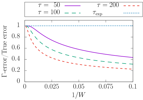
Figure 1: We show the approach to the true error in the $\Gamma$-method as a function of the summation window $W$ for three values of $\tau$. In all cases the autocorrelation function is assumed to follow a simple exponential decay $\Gamma(t)=e^{-|t|/\tau}$ (see appendix A). The asymptotic convergence is exponential, but in many practical situations we are far from this asymptotic behavior. As proposed in [3] we can account for the slow modes in the analysis using eq. (2.18) (corresponding to the line labeled $\tau_{\rm exp}$). In this very simple example (where the autocorrelation function has a single contribution) this procedure gives the correct error estimation for any window size and value of $\tau$.

Although this is a sensible choice, it has been noted [3] that in many practical situations in lattice computations $\tau_{\rm exp}^{\alpha}$ and $\tau_{\rm int}^{\alpha}$ are in fact very different. In these cases the summation window $W^{\alpha}_{F}$ cannot be taken much larger than $\tau^{\alpha}_{\rm exp}$, and one risks ending up underestimating the errors (see figure 1). An improved estimate for $\tau_{\rm int}^{\alpha}$ was proposed for these situations. First the autocorrelation function $\rho_{F}^{\alpha}(t)$ is summed explicitly up to $W_{F}^{\alpha}$. This value has to be large, but such that $\rho_{F}^{\alpha}(W_{F}^{\alpha})$ is statistically different from zero. For $t>W_{F}^{\alpha}$ we assume that the autocorrelation function is basically given by the slowest mode $\rho_{F}^{\alpha}(t)\sim\exp(-|t|/\tau_{\rm exp}^{\alpha})$ and explicitly add the remaining tail to the computation of $\tau_{\rm int}^{\alpha}$. The result of this operation can be summarized in the formula

$$\tau_{\rm int}^{\alpha}=\frac{1}{2}+\sum_{t=1}^{W^{\alpha}_{F}}\rho_{F}^{\alpha}(t)+\tau_{\rm exp}^{\alpha}\rho_{F}^{\alpha}(W_{F}^{\alpha}+1)\,.$$ (2.18)

The original proposal [3] consists in adding the tail to the autocorrelation function at a point where $\rho_{F}(t)$ is three standard deviations away from zero, and use the error estimate (2.18) as an upper bound on the error. On the other hand recent works of the ALPHA collaboration attach the tail when the signal in $\rho_{F}(t)$ is about to be lost (i.e. $\rho_{F}(t)$ is 1-2 standard deviations away from zero) and use eq. (2.18) as the error estimate (not as an upper bound). This last option seems more appealing to the author.

All these procedures require an estimate of $\tau_{\rm exp}^{\alpha}$. This is usually obtained by inspecting large statistics in cheaper simulations (pure gauge, coarser lattice spacing, …). The interested reader is invited to consult the original references [3, 5] for a full discussion.

2.2.1 Notes on the practical implementation of the $\Gamma$-method

In practical implementations of the $\Gamma$-method, as suggested in [1], it is convenient to store the mean and the projected fluctuations per ensemble of an observable

$$\bar{F}=f(\bar{a}_{i}^{\alpha})\,,\qquad\delta_{F}^{\alpha}(t)=\sum_{i}\bar{f}_{i}^{\alpha}\delta_{i}^{\alpha}(t)\,.$$ (2.19)

Note that observables that are functions of other derived observables are easily analyzed. For example, if we are interested in

$$G=g(f(A_{i}^{\alpha}))\,,$$ (2.20)

we first compute

$$\bar{F}=f(\bar{a}_{i}^{\alpha})\,,\qquad\delta_{F}^{\alpha}(t)=\sum_{i}\bar{f}_{i}^{\alpha}\delta_{i}^{\alpha}(t)\,.$$ (2.21)

Now to determine $G$ we only need an extra derivative $\bar{g}_{F}=\partial_{F}g\Big{|}_{\bar{F}}$, since

$$\bar{G}=g(\bar{F})=g(f(\bar{a}_{i}^{\alpha}))\,,\qquad\delta_{G}^{\alpha}(t)=\bar{g}_{F}\delta_{F}^{\alpha}(t)=\sum_{i}\bar{g}_{F}\bar{f}_{i}^{\alpha}\delta_{i}^{\alpha}(t)=\sum_{i}\bar{g}_{i}^{\alpha}\delta_{i}^{\alpha}(t)\,,$$ (2.22)

with $\bar{g}_{i}^{\alpha}=\partial_{i}^{\alpha}g|_{\bar{a}_{i}^{\alpha}}$.

At this point the difference between a primary and a derived observable is just convention: any primary observable can be considered a derived observable defined with some identity function. It is also clear that the means and the fluctuations are all that is needed to implement linear propagation of errors in the $\Gamma$-method.

Finally, we emphasize that computing derivatives of arbitrary functions lies at the core of the $\Gamma$-method. In [1, 3] a numerical evaluation of the derivatives is used. Here we propose to use AD techniques for reasons of efficiency and robustness, but before giving details on AD we will comment on the differences between the $\Gamma$-method and the popular methods based on binning and resampling.

2.3 Binning techniques

Figure 2: Blocks of data are averaged to produce a new data set with less autocorrelations. No matter how large the bins are, adjacent bins have always data that are very close in MC time.

Resampling methods (bootstrap, jackknife) usually rely on binning to reduce the autocorrelations of the data. One does not resample the data itself, but bins of data. The original measurements $a_{i}^{\alpha}(t)$ are first averaged in blocks of size $N_{B}$ (see figure 2)

$$b_{i}^{\alpha}(w)=\frac{1}{N_{B}}\sum_{t=1+(w-1)N_{B}}^{wN_{B}}a_{i}^{\alpha}(t)\,,\qquad(w=1,\dots,N_{\alpha}/N_{B})\,.$$ (2.23)

This blocked data is then treated like independent measurements and resampled, either with replacement in bootstrap techniques or by just leaving out each observation (jackknife).

How good is the assumption that blocks are independent? A way to measure this is to determine the autocorrelation function of the blocked data (see appendix A.1). In [1] it is shown that the leading term for large $N_{B}$ in the integrated autocorrelation time of the binned data is $\mathcal{O}(1/N_{B})$. The autocorrelation function decays exponentially at large MC time, but the fact that adjacent bins have always data that are very close in MC time (see fig. 3) transforms this expected exponential suppression in a power law.

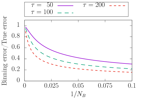
Figure 3: We show the approach to the true error by binning as a function of the bin size $N_{B}$ for three values of $\tau$. In all cases the autocorrelation function is assumed to follow a simple exponential decay $\Gamma(t)=e^{-|t|/\tau}$ (see appendix A). The asymptotic convergence is slow ($\mathcal{O}(1/N_{B})$). Moreover in many practical situations we are far from this asymptotic behavior.

In practice it is difficult to have bins of size much larger than the exponential autocorrelation times. In this situation one is far from the asymptotic $\mathcal{O}(1/N_{B})$ scaling and binning severely underestimates the errors. An instructive example is to just consider a data with simple autocorrelation function $\Gamma(t)=e^{-|t|/\tau}$ (see appendix A.1). Figure 3 shows the approach to the true error as a function of the bin size for different values of $\tau$.

This example should be understood as a warning, and not as an academic example: in state of the art lattice QCD simulations it is not uncommon to simulate at parameter values where $\tau_{\rm exp}\sim 100-200$, and it is fairly unusual to have statistics that allow for bins of sizes larger than 50-100. We end up commenting that the situation in the $\Gamma$-method is better for two reasons. First the truncation errors are exponential instead of power-like when enough data is available. Second (and more important), in the cases where the statistics is not much larger than the exponential autocorrelation times, an improved estimate like eq. (2.18) is only available for the $\Gamma$-method.

2.4 The $\Gamma$-bootstrap method

Conceptually there is no need to use binning techniques with resampling. Binning is only used to tame the autocorrelations in the data, and as we have seen due to the current characteristics of the lattice QCD simulations it seriously risks underestimating the errors.

Resampling is a tool for error propagation that automatically takes into account the correlations among different observables. A possible analysis strategy consist in using the $\Gamma$-method to determine the errors of the primary observables, and use resampling techniques for error propagation.

The $N_{\rm p}\times N_{\rm p}$ covariance matrix among the primary observables $A_{i}^{\alpha}$ can be estimated by

$${\rm cov}(A_{i}^{\alpha},A_{j}^{\beta})\approx\frac{1}{N_{\alpha}}\left[\Gamma_{ij}^{\alpha\beta}(0)+2\sum_{t=1}^{W^{\alpha}}\Gamma_{ij}^{\alpha\beta}(t)\right]\,.$$ (2.24)

The effect of large tails in the autocorrelation functions can also be accounted for in the determination of this covariance matrix by using

$${\rm cov}(A_{i}^{\alpha},A_{j}^{\beta})\approx\frac{1}{N_{\alpha}}\left[\Gamma_{ij}^{\alpha\beta}(0)+2\sum_{t=1}^{W^{\alpha}}\Gamma_{ij}^{\alpha\beta}(t)+2\tau_{\rm exp}^{\alpha}\Gamma_{ij}^{\alpha\beta}(W^{\alpha}+1)\right]\,.$$ (2.25)

In the previous formulas the window $W^{\alpha}$ can be chosen with similar criteria as described in section 2. Different diagonal entries $i=j$ might give different values for the window $W^{\alpha}_{i}$. For the case of eq. (2.24), the values $W_{i}^{\alpha}$ are chosen with the criteria described in [1], and conservative error estimates are obtained by using

$$W^{\alpha}=\max_{i}\{W_{i}^{\alpha}\}\,.$$ (2.26)

On the other hand for the case of eq. (2.25) we choose $W_{i}^{\alpha}$ according to the criteria discussed before eq. (2.18), and we use

$$W^{\alpha}=\min_{i}\{W_{i}^{\alpha}\}\,.$$ (2.27)

Once the covariance matrix is known, one can generate bootstrap samples following a multivariate Gaussian distribution with the mean of the observables $\bar{a}_{i}^{\alpha}$ as mean, and the covariance among observables as covariance. These bootstrap samples are used for the analysis as in any resampling analysis where the samples come from binning. We will refer to this analysis technique as $\Gamma$-bootstrap.

It is clear that if each primary observable is measured in a different ensemble the covariance matrix ${\rm cov}(A_{i}^{\alpha},A_{j}^{\beta})$ is diagonal (cf. equation (2.12)). In this case the bootstrap samples are generated by just generating independent random samples $\mathcal{N}(\bar{a}_{i}^{\alpha},\sigma^{2}(a_{i}^{\alpha}))$ for each observable. Moreover in this particular case the analysis of the data will give completely equivalent results as using the $\Gamma$-method. This is more clearly seen by looking at equation (2.22): any derived observable will have just the same set of autocorrelation functions except for a different scaling factor that enters the error determination in a trivial way.

				Binning error/True error
Observable	Value	$\lambda_{k}$	$\tau_{\rm int}$	$N_{B}=10$	$N_{B}=25$	$N_{B}=50$
$x$	2.00(7)	$(1.08,0.08,0.05,0.0)$	4.5	0.75	0.87	0.91
$y$	1.86(8)	$(1.00,0.15,0.0,0.05)$	6.1	0.65	0.76	0.82
$z=x/y$	1.075(14)	$(0.0025,-0.044,0.027,-0.029)$	56.1	0.25	0.36	0.48

Table 1: Large autocorrelation times can show up on derived observables even in cases where the primary observables have all small autocorrelations. The error in the column labeled “value” shows the exact value of the observable and an error computed assuming a sample of length 2000. The values of $\lambda_{k}$, together with $\tau_{k}=(4.0,100.0,2.0,3.0)$ give the autocorrelation functions $\Gamma(t)=\sum_{k}\lambda_{k}^{2}e^{-|t|/\tau_{k}}$ (see appendix A).

But when several observables determined on the same ensembles enter in the analysis, results based on this $\Gamma$-bootstrap approach are not equivalent to analysis based on the $\Gamma$-method. In resampling methods we loose all information on autocorrelations when we build the bootstrap samples. When combining different observables from the same ensembles the slow modes of the MC chain can be enhanced. Large autocorrelations may show up in derived observables even in cases when the primary observables have all small integrated autocorrelation times. Table 1 shows an example where the ratio of two primary observables shows large autocorrelation times ($\tau_{\rm int}=56$) even in the case where the two primary observables have relatively small autocorrelation times ($\tau_{\rm int}=4.5$ and $\tau_{\rm int}=6.1$). Note also that the derived observable is very precise (the error is 6 times smaller than those of the primary observables).

Once more this example should not be considered as an academic example. Profiting from the correlations among observables to obtain precise results lies at the heart of many state of the art computations. As examples we can consider the ratio of decay constants ($F_{K}/F_{\pi}$ plays a central role in constraining CKM matrix elements for example) or the determination of isospin breaking effects. In these cases there is always the danger that the precise derived observable shows larger autocorrelations than the primary observables.

While one loses information on the autocorrelations for derived observables (only a full analysis with the $\Gamma$-method has access to this information), the large truncation errors expected from binning are avoided by using a combination of the $\Gamma$-method and resampling techniques for error propagation. Therefore this analysis technique should always be preferred over analysis using binning techniques.

3 Automatic differentiation

At the heart of linear error propagation with the $\Gamma$-method lies the computation of derivatives of arbitrary functions (see eq. (2.22)). In this work we propose to use Automatic differentiation (AD) to compute these derivatives.

AD is a set of techniques to evaluate derivatives of functions. A delicate point in numerical differentiation is the choice of step size. If chosen too small, one will get large round-off errors. One can also incur in systematic errors if the step size used is too large. AD is free both of systematic and round-off errors: derivatives of arbitrary functions are computed to machine precision. At the core of the idea of using AD to compute derivatives lies the fact that any function, even complicated iterative algorithms, are just a series of fundamental operations and the evaluation of a few intrinsic functions. In AD the derivatives of these fundamental operations and few intrinsic functions are hard-coded, and the derivatives of complicated functions follow from recursively applying the basic rules.

In AD the decomposition of a derivative in derivatives of the elementary operations/functions is fundamental. A central role is played by the chain rule. If we imagine a simple composition of functions

$$y=f_{3}(f_{2}(f_{1}(x)))\,,$$ (3.1)

and we are interested in the derivative ${\rm d}y/{\rm d}x$ we can define the following intermediate variables

$$z_{0}=x,\quad z_{1}=f_{1}(x),\quad z_{2}=f_{2}(z_{1}),\quad z_{3}=f_{3}(z_{2})\,.$$ (3.2)

The chain rule gives for the derivative ${\rm d}y/{\rm d}x$ the following expression

$$\frac{{\rm d}y}{{\rm d}x}=\frac{{\rm d}y}{{\rm d}z_{2}}\frac{{\rm d}z_{2}}{{\rm d}z_{1}}\frac{{\rm d}z_{1}}{{\rm d}z_{0}}\,.$$ (3.3)

AD can be applied to compute the previous derivative by using two modes: reverse accumulation and forward accumulation. In reverse accumulation [11], one starts the chain rule with the variable that is being differentiated ($y$ in the previous example), and proceeds to compute the derivatives recursively. On the other hand, forward accumulation determines the derivatives with respect to the independent variable first ($x$ in our example). The reader interested in the details is invited to consult the literature on the subject [12].

Although more efficient for some particular problems, the implementation of reverse accumulation AD is usually involved (see [12] for a full discussion). On the other hand the implementation of forward accumulation is more straightforward and it is naturally implemented by overloading the fundamental operations and functions in languages that support such features. For the particular applications described in this work, most of the time of the analysis is spent in computing the projected fluctuations eq. (2.19) and in computing the autocorrelation function eq. (2.12), therefore the particular flavor of AD used does not influence the efficiency of the analysis code. With these general points in mind, in the following sections we will introduce a particularly convenient and simple implementation of forward accumulation AD [13], that is suitable for all the applications described in this work.

3.1 Forward accumulation AD and hyper-dual numbers

In forward accumulation, the order for evaluating derivatives corresponds to the natural order in which the expression is evaluated. This just asks to be implemented by extending the operations ($+,-,*,/,\dots$) and intrinsic functions ($\sin,\cos,\exp,\dots$) from the domain of the real numbers.

Hyper-dual numbers [13] are represented as 4-components vectors of real numbers $\tilde{x}=\bm{\langle\,}x_{1}\bm{,}\,x_{2}\bm{,}\,x_{3}\bm{,}\,x_{4}\bm{\,\rangle}$. They form a field with operations

$$\tilde{x}\pm\tilde{y} = \bm{\langle\,}x_{1}\pm y_{1}\bm{,}\,x_{2}\pm y_{2}\bm{,}\,x_{3}\pm y_{3}\bm{,}\,x_{4}\pm y_{4}\bm{\,\rangle}\,,$$ (3.4)

$$\tilde{x}\tilde{y} = \bm{\langle\,}x_{1}y_{1}\bm{,}\,x_{1}y_{2}+x_{2}y_{1}\bm{,}\,x_{1}y_{3}+x_{3}y_{1}\bm{,}\,x_{1}y_{4}+x_{4}y_{1}+x_{2}y_{3}+x_{3}y_{2}\bm{\,\rangle}\,,$$ (3.5)

$$\tilde{x}^{-1} = \bm{\langle\,}1/x_{1}\bm{,}\,-x_{2}/x_{1}^{2}\bm{,}\,-x_{3}/x_{1}^{2}\bm{,}\,2x_{2}x_{3}/x_{1}^{3}-x_{4}/x_{1}^{2}\bm{\,\rangle}\,.$$ (3.6)

Arbitrary real functions $f:\mathbb{R}\to\mathbb{R}$ are promoted to hyper-dual functions by the relation

$$\tilde{f}(\tilde{x})=\bm{\langle\,}f(x_{1})\bm{,}\,f^{\prime}(x_{1})x_{2}\bm{,}\,f^{\prime}(x_{1})x_{3}\bm{,}\,x_{4}f^{\prime}(x_{1})+x_{2}x_{3}f^{\prime\prime}(x_{1})\bm{\,\rangle}\,.$$ (3.7)

Note that the function and its derivatives are only evaluated at the first component of the hyper-dual argument $x_{1}$. In contrast with the techniques of symbolic differentiation, AD only gives the values of the derivatives of a function in one specific point. We also stress that the usual field for real numbers is recovered for hyper-real numbers of the form $\tilde{x}=\bm{\langle\,}x_{1}\bm{,}\,0\bm{,}\,0\bm{,}\,0\bm{\,\rangle}$ (i.e. the real numbers are a sub-field of the hyper-dual field).

Performing any series of operations in the hyper-dual field, the derivatives of any expression are automatically determined at the same time as the value of the expression itself. It is instructive to explicitly check the case of a simple function composition

$$y=f(g(x))\,.$$ (3.8)

If we evaluate this at the hyper-real argument $\tilde{x}$, it is straightforward to check that one gets

$$\tilde{z}=\tilde{g}(\tilde{x}) = \bm{\langle\,}g(x_{1})\bm{,}\,g^{\prime}(x_{1})x_{2}\bm{,}\,g^{\prime}(x_{1})x_{3}\bm{,}\,x_{4}g^{\prime}(x_{1})+x_{2}x_{3}g^{\prime\prime}(x_{1})\bm{\,\rangle}\,.$$ (3.9)

$$\tilde{y}=\tilde{f}(\tilde{z}) = \bm{\langle\,}f(z_{1})\bm{,}\,f^{\prime}(z_{1})z_{2}\bm{,}\,f^{\prime}(z_{1})z_{3}\bm{,}\,z_{4}f^{\prime}(z_{1})+z_{2}z_{3}f^{\prime\prime}(z_{1})\bm{\,\rangle}$$ (3.10)

$$= \bm{\langle\,}f(g(x_{1}))\bm{,}f^{\prime}(g(x_{1}))g^{\prime}(x_{1})x_{2}\bm{,}f^{\prime}(g(x_{1}))g^{\prime}(x_{1})x_{3}\bm{,}$$ (3.12)

$$f^{\prime}(g(x_{1}))(x_{4}g^{\prime}(x_{1})+x_{2}x_{3}g^{\prime\prime}(x_{1}))+g^{\prime 2}(x_{1})f^{\prime\prime}(g(x_{1}))x_{2}x_{3}\bm{\,\rangle}\,.$$

Now if we set $\tilde{x}=\bm{\langle\,}x_{1}\bm{,}\,1\bm{,}\,1\bm{,}\,0\bm{\,\rangle}$, we get $y^{\prime}$ as the second/third component of $\tilde{y}$, and $y^{\prime\prime}$ as the fourth component of $\tilde{y}$.

3.2 Functions of several variables

The extension to functions of several variables is straightforward. Each of the real arguments of the function is promoted to an hyper-dual number. The hyper-dual field allows the computation of the gradient and the Hessian of arbitrary functions.

For a function of several variables $f(\mathbf{x})$, after promoting all its arguments to the hyper-dual field we get the hyper-dual function $\tilde{f}(\tilde{\mathbf{x}})$. Partial derivatives of the original function $\partial_{i}f(\mathbf{x})$ and the Hessian $\partial_{i}\partial_{j}f(\mathbf{x})$ can be obtained using appropriate hyper-dual arguments (see table 2 for an explicit example with a function of two variables).

$\tilde{x}$	$\tilde{y}$	$\tilde{f}(\tilde{x},\tilde{y})$
$\bm{\langle\,}x_{1}\bm{,}\,1\bm{,}\,1\bm{,}\,0\bm{\,\rangle}$	$\bm{\langle\,}y_{1}\bm{,}\,0\bm{,}\,0\bm{,}\,0\bm{\,\rangle}$	$\bm{\langle\,}f\bm{,}\,\partial_{x}f\bm{,}\,\partial_{x}f\bm{,}\,\partial_{x}^{2}f\bm{\,\rangle}$
$\bm{\langle\,}x_{1}\bm{,}\,1\bm{,}\,0\bm{,}\,0\bm{\,\rangle}$	$\bm{\langle\,}y_{1}\bm{,}\,0\bm{,}\,1\bm{,}\,0\bm{\,\rangle}$	$\bm{\langle\,}f\bm{,}\,\partial_{x}f\bm{,}\,\partial_{y}f\bm{,}\,\partial_{x}\partial_{y}f\bm{\,\rangle}$
$\bm{\langle\,}x_{1}\bm{,}\,0\bm{,}\,0\bm{,}\,0\bm{\,\rangle}$	$\bm{\langle\,}y_{1}\bm{,}\,1\bm{,}\,1\bm{,}\,0\bm{\,\rangle}$	$\bm{\langle\,}f\bm{,}\,\partial_{y}f\bm{,}\,\partial_{y}f\bm{,}\,\partial_{y}^{2}f\bm{\,\rangle}$

Table 2: Example output for a function of two variables $f(x,y)$ after promoting the arguments to hyper-real numbers. In the third column the function and all derivatives are evaluated at $(x_{1},y_{1})$.

4 Applications of AD to the analysis of MC data

The common approach to error propagation in a generic function consists in examining how the function behaves when the input is modified within errors. For example in resampling techniques the target function is evaluated for each sample, and the spread in the function values is used as an estimate of the error in the value of the function. This approach is also used in cases where the function is a complicated iterative procedure. The main example being error propagation in fit parameters, that is usually performed by repeating the fit procedure for slightly modified values of the data points.

AD techniques propose an interesting alternative to this general procedure: just performing every operation in the field of hyper-dual numbers will give the derivatives necessary for error propagation exactly, even if we deal with a complicated iterative algorithm (section 5.1 contains an explicit example). This is relatively cheap numerically. For example in the case of functions of one variable the numerical cost is roughly two times the cost of evaluating the function if one is interested in the value of the function and its first derivative, and between three and four times if one is interested in the first and second derivatives. This has to be compared with the three evaluations that are needed to obtain the value of the function and an estimate of the first derivative using a symmetric finite difference, or the $\mathcal{O}(1000)$ evaluations that are used in a typical resampling approach.

In the rest of this section we will see that in many iterative algorithms error propagation can be simplified. The most interesting example concerns the case of error propagation in fit parameters: we will see that it is enough to compute the second derivative of the $\chi^{2}$ function at the minima. As a warm up example, we will consider the simpler (but also interesting) case of error propagation in the root of a non-linear function.

4.1 Error propagation in the determination of the root of a function

A simple example is finding a root of a non-linear function of one real variable. We are interested in the case when the function depends on some data $d_{a}\,(a=1,\dots,N_{\rm data})$ that are themselves Monte Carlo observables, $f(x;d_{a})$. In this case the error in the MC data $d_{a}$ propagates into an error of the root of the function. We assume that for the central values of the data $\bar{d}_{a}$ the root is located at $\bar{x}$

$$f(\bar{x};\bar{d}_{a})=0\,.$$ (4.1)

For error propagation we are interested in how much changes the position of the root when we change the data. This “derivative” can be easily computed. When we shift the data around its central value $\bar{d}_{a}\to\bar{d}_{a}+\delta d_{a}$, to leading order the function changes to

$$f(x;\bar{d}_{a}+\delta d_{a})=f(x;\bar{d}_{a})+\partial_{a}f\Big{|}_{(x;\bar{d}_{a})}\delta d_{a}\qquad(\partial_{a}\equiv\partial/\partial d_{a})\,.$$ (4.2)

This function will no longer vanish at $\bar{x}$, but at a slightly shifted value $x=\bar{x}+\delta x$. Again to leading order

$$f(\bar{x}+\delta x;\bar{d}_{a}+\delta d_{a})=f(\bar{x};\bar{d}_{a})+\partial_{x}f\Big{|}_{(\bar{x};\bar{d}_{a})}\delta x+\partial_{a}f\Big{|}_{(\bar{x};\bar{d}_{a})}\delta d_{a}=0\,.$$ (4.3)

This allows to obtain the derivative of the position of the root with respect to the data

$$\frac{\delta x}{\delta d_{a}}=-\frac{\partial_{a}f}{\partial_{x}f}\Big{|}_{(\bar{x};\bar{d}_{a})}\,.$$ (4.4)

That is the quantity needed for error propagation. Note that in practical applications the iterative procedure required to find the root (i.e. Newton’s method, bisection, …) is only used once (to find the position of the root). Error propagation only needs the derivatives of the target function at $(\bar{x},\bar{d}_{a})$.

4.2 Error propagation in fit parameters

In (non-linear) least squares one is usually interested in finding the values of some parameters $p_{i}\,(i=1,\dots,N_{\rm parm})$ that minimize the function

$$\chi^{2}(p_{i};d_{a})\,,\qquad p_{i}\,(i=1,\dots,N_{\rm parm})\,,\quad d_{a}\,(a=1,\dots,N_{\rm data})\,.$$ (4.5)

Here $d_{a}$ are the data that is fitted. In many cases the explicit form of the $\chi^{2}$ is

$$\chi^{2}=\sum_{a=1}^{N_{\rm data}}\left(\frac{f(x_{a};p_{i})-y_{a}}{\sigma(y_{a})}\right)^{2}\,,$$ (4.6)

where $f(x_{a};p_{i})$ is a function that depends on the parameters $p_{i}$, and $y_{a}$ are the data points (represented by $\{d_{a}\}$ in eq. (4.5)). The result of the fit is some parameters $\bar{p}_{i}$ that make $\chi^{2}(\bar{p}_{i};\bar{d}_{a})$ minimum for some fixed values of the data $\bar{d}_{a}$.

When propagating errors in a fit we are interested in how much the parameters change when we change the data. This “derivative” is defined by the implicit condition that the $\chi^{2}$ has to stay always at its minimum. If we shift the data $d_{a}\to\bar{d}_{a}+\delta d_{a}$ we have to leading order

$$\chi^{2}(p_{i};\bar{d}_{a}+\delta d_{a})=\chi^{2}(p_{i};\bar{d}_{a})+\partial_{a}\chi^{2}\Big{|}_{(p_{i};\bar{d}_{a})}\,\delta d_{a}\,,\qquad(\partial_{a}\equiv\partial/\partial d_{a})\,.$$ (4.7)

this function will no longer have its minimum at $\bar{p}_{i}$ but will be shifted by an amount $\delta p_{i}$. Minimizing with respect to $p_{i}$ and expanding at $p_{i}=\bar{p}_{i}$ to leading order one obtains the condition

$$\partial_{j}\partial_{i}\chi^{2}\Big{|}_{(\bar{p}_{i};\bar{d}_{a})}\delta p_{j}+\partial_{i}\partial_{a}\chi^{2}\Big{|}_{(\bar{p}_{i};\bar{d}_{a})}\,\delta d_{a}=0\,,\qquad(\partial_{i}\equiv\partial/\partial p_{i})\,.$$ (4.8)

Defining the Hessian of the $\chi^{2}$ at the minimum

$$H_{ij}=\partial_{j}\partial_{i}\chi^{2}\Big{|}_{(\bar{p}_{i};\bar{d}_{a})}\,,$$ (4.9)

we can obtain the derivative of the fit parameters with respect to the data 

$$\frac{\delta p_{i}}{\delta d_{a}}=-\sum_{j=1}^{N_{\rm parm}}(H^{-1})_{ij}\partial_{j}\partial_{a}\chi^{2}\Big{|}_{(\bar{p}_{i};\bar{d}_{a})}\,.$$ (4.10)

Once more the iterative procedure is only used one time (to find the central values of the fit parameters), and error propagation is performed by just evaluating derivatives of the $\chi^{2}$ function at $(\bar{p}_{i},\bar{d}_{a})$.

5 Worked out example

As an example of the analysis techniques described in the text we are going to study a simple non-linear fit. We want to describe the functional form $\tilde{y}(x)$ in the region $x\in[1,5]$. For this purpose we have measured five values of $\tilde{y}$ at five values of $x=1.0,2.0,3.0,4.0,5.0$ respectively. We are going to assume that the data is well described by the model

$$y=\log(n+x)+\sin(mx)\,,\qquad(\text{with }y=Z\tilde{y})\,.$$ (5.1)

The factor $Z$ is also part of the available measurements. Once the parameters $n$ and $m$ are determined by fitting our data $(x_{i},\tilde{y}_{i})$ we will have a parametrization of the function $\tilde{y}(x)$. Note that equation (5.1) describes a highly non-linear function, both in the fit parameters and the independent variable $x$.

In the terminology of section 2 we have six primary observables (the common factor $Z$ and the five $\tilde{y}_{i}$) measured each of them in a different ensemble

$$A_{1}^{1}=\tilde{y}_{1},\,A_{1}^{2}=\tilde{y}_{2},\,A_{1}^{3}=\tilde{y}_{3},\,A_{1}^{4}=\tilde{y}_{4},\,A_{1}^{5}=\tilde{y}_{5},\,A_{1}^{6}=Z\,.$$ (5.2)

The exact values of these primary observables together with the parameters used to generate the MC data are described in table 3. As examples of quantities of interest, we will focus on obtaining the values and uncertainties of

1. The fit parameters $n,m$.

2. The value of the fitted function at $x=3/2$

   $$I=\log\left(\frac{3}{2}+n\right)+\sin\left(\frac{3m}{2}\right)$$ (5.3)

Note that these quantities are derived observables in the terminology of section 2 (i.e. functions of the primary observables, defined via the fitting procedure).

	$\tilde{y}_{1}$	$\tilde{y}_{2}$	$\tilde{y}_{3}$	$\tilde{y}_{4}$	$\tilde{y}_{5}$	$Z$
Value	0.9021	1.5133	1.9319	2.1741	2.2508	1.2
$\tau$	2	4	6	8	10	100
$\lambda$	1	1	1	1	1	0.1
$\tau_{\rm int}$	2.0415	4.0208	6.0139	8.0104	10.008	100.00

Table 3: Primary observables of our worked out example. The row labeled Value shows the exact value of the observable. Rows $\tau$ and $\lambda$ show the values of the parameters used to generate the MC samples along the lines discussed in appendix A (the MC data follows a simple autocorrelation function $\sim e^{-|t|/\tau}$). Row $\tau_{\rm int}$ shows the exact value of the integrated autocorrelation time of the observable.

In order to estimate our derived observables, we have at our disposal 2000 MC measurements for each of the six primary observables. Table 4 shows the estimates of these six primary observables using different analysis techniques: on one hand the $\Gamma$-method, where we use the improved error estimate (eq (2.18)) with $\tau_{\rm exp}=100$ for the analysis of the observable $Z$, and the usual automatic window procedure described in [1] with $S_{\tau}=2.0$ for the five observables $\tilde{y}_{i}$. On the other hand we use the more common binning/resamplnig techniques with different bin sizes.

	$\Gamma$-method		Binning
			$N_{\rm bin}=10$	$N_{\rm bin}=25$	$N_{\rm bin}=50$
Obs.	$\tau_{\rm exp}$					Error
$\tilde{y}_{1}$	0	0.881(50)	0.881(43)	0.881(49)	0.881(54)	0.045
$\tilde{y}_{2}$	0	1.448(47)	1.448(47)	1.448(45)	1.448(46)	0.063
$\tilde{y}_{3}$	0	1.981(91)	1.981(62)	1.981(78)	1.981(85)	0.078
$\tilde{y}_{4}$	0	2.21(11)	2.206(57)	2.206(72)	2.206(93)	0.090
$\tilde{y}_{5}$	0	2.309(96)	2.309(58)	2.309(76)	2.309(75)	0.100
$Z$	100	$1.188(40)$	$1.1878(75)$	$1.188(12)$	$1.188(16)$	0.032

Table 4: Estimates of the values of the primary observables $\tilde{y}_{i},Z$ using different analysis techniques. The last column labeled “error” quotes the exact error of the observable assuming a sample of length 2000 (see appendix A). The analysis of the primary observables is performed with different techniques: the $\Gamma$-method, where the slow mode in observable $Z$ is taken into account as describd in eq. (2.18), and the more traditional binning/resampling where we have choosen different bin sizes.

The strategy to determine the derived observables $n,m,I$ is the usual one: we fit our data by minimizing the $\chi^{2}$ function

$$\chi^{2}=\sum_{a=1}^{5}\left(\frac{\log(n+x_{a})+\sin(mx_{a})-y_{a}}{\sigma(y_{a})}\right)^{2}\,,\qquad(y_{a}=Z\tilde{y}_{a})\,.$$ (5.4)

We will use different approaches to determine the fit parameters and $I$.

1. First we will use our proposal of section 4.2: We use any fitting routine, and once the minimum is found, the Hessian is determined with AD techniques and linear error propagation is performed. We will perform the analysis including the tail in the autocorrelations function of the slow observable $Z$ (with $\tau_{\rm exp}=100$). The tail will be added when $\rho(t)$ is 1.5 times its error. For the other observables we will just assume that we have enough data so that truncation effects have negligible systematics.

2. As is clear from the discussion in section 2.3 binning methods tend to underestimate the true error. In section 2.4 we detailed the $\Gamma$-bootstrap method, where errors of primary observables are computed with the $\Gamma$-method and resampling is used for error propagation. Since observable $Z$ is a primary observable we can add a tail to the autocorrelation function using $\tau_{\rm exp}=100$. The tail will be added when $\rho(t)$ is 1.5 times its error.

3. Finally we have used the more common binning and resampling approach. We use bins of size 10, 25, 50 so that we are left with 200, 80 and 40 measurement respectively. These measurements are resampled (we use 2000 samples) with replacement (bootstrap) in order to perform the usual error analysis.

We note however that comparing binning with the $\Gamma$-method is not the main purpose of this section. A detailed comparison requires to either push the approach outlined in appendix A to compare error determinations in this model, or to repeat the same analysis with several data sets that only differ in the random number seed. These comparisons are available in the literature [1, 3, 5]. Here we will focus on how to perform the analysis with the $\Gamma$-method when different ensembles enter our error determination and in the use of AD techniques.

The results of this small experiment are summarized in table 5. As the reader can see the $\Gamma$-method together with linear error propagation using AD techniques is much more efficient in terms of computer time. It also leads to conservative error estimates. Even in this mild case, where our primary measured observables have most of its contributions coming from fast Monte Carlo modes ($\tau\sim 2-10$), binning methods severely underestimate the errors unless one has access to very large bin sizes. This is of course expected on theoretical grounds [1] (see appendix A.1).

		$\Gamma$-method (AD)	$\Gamma$-bootstrap	Binning + bootstrap
Qauntity	Value	$\tau_{\rm exp}=100$		$N_{\rm bin}=10$	$N_{\rm bin}=25$	$N_{\rm bin}=50$
$n$	1.0	0.98(19)	0.98(21)	0.97(12)	0.97(15)	0.97(17)
$m$	0.4	0.365(45)	0.364(56)	0.372(32)	0.367(41)	0.365(44)
$I$	1.4809…	1.429(62)	1.428(61)	1.435(35)	1.429(39)	1.425(43)
Time		1	$\sim 250$

Table 5: Results for the derived observables $n,m$ and $I$ using different analysis methods. The column “Value” gives the exact value of the parameters. We show the estimates coming from different analysis techniques. Note that binning severely underestimates the errors unless one has access to very large bins of data. As expected for this case the mixed $\Gamma$-bootstrap approach for the error propagation shows no difference from the results obtained via the $\Gamma$-method (see the discussion on the text). Error propagation using AD techniques, where the fit is only performed once, is much more efficient in terms of computing time. (Times were measured by repeating the analysis 100-1000 times in a standard laptop. The timing does not pretend to be accurate, just to give an idea of the order of magnitude).

The $\Gamma$-bootstrap method (cf. section 2.4) is a safe alternative to the full analysis using the $\Gamma$-method in this case. Note that we have only one primary observable from each ensemble, and therefore there is no possibility of any cancelation that would uncover some large autocorrelations (see section 2.4). The $\Gamma$-method is still faster due to the fact that resampling methods have to perform the fit many times (2000 in the example above), while AD techniques allow to perform the error propagation with only a single minimization. On the other hand the $\Gamma$-method requires to keep track of all the fluctuations per ensemble (in the example above the fit parameters are derived observables with 2000 fluctuations for each of the 6 primary observables) and perform some FFTs to do the necessary convolutions needed to determine the autocorrelation function. Still the analysis with the $\Gamma$-method is around two orders of magnitude faster than resampling techniques.

One of the advantages of the $\Gamma$-method is that the fluctuations per ensemble are available even for complicated derived observables. This gives access to the contribution of each ensemble to the total error (see equation (2.16)), as well as to the the fluctuations of the derived observable with respect to any of the ensembles. Focusing our attention in observable $I$ we see (cf. table 6) that the largest contribution to the error comes from the observable $Z$, while ensembles 3, 4 and 5 contribute very little. Figure 4 shows the MC history of the fluctuations in $I$ for each Monte Carlo ensemble. The main source of error, has in fact fluctuations with a small amplitude, but the large exponential autocorrelation time in this ensemble makes it the main source of error in our determination of $I$.

	Contribution to error
Quantity	Ensemble 1	Ensemble 2	Ensemble 3	Ensemble 4	Ensemble 5	Ensemble $Z$
$n$	35.08 %	0.62 %	1.29 %	0.68 %	22.07 %	40.27 %
$m$	9.40 %	22.98 %	14.35 %	0.04 %	53.19 %	0.04 %
$I$	21.36 %	11.89 %	4.32 %	0.72 %	0.70 %	61.01 %

Table 6: Details of the analysis for the quantity that correspond to the interpolation of the fitted function at $x=3/2$. We observe that despite being an interpolation between the data of ensembles 1 and 2, the largest contribution to the error comes from the parameter $Z$ (Note that $Z$ has the smaller relative uncertainty in table 4).

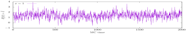
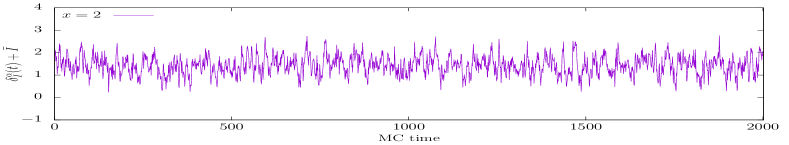
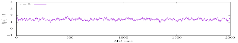
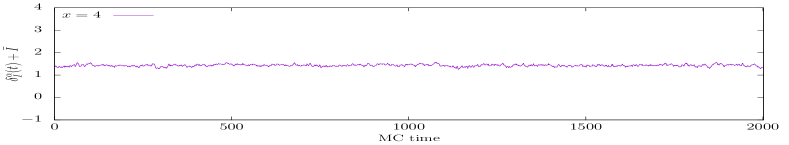
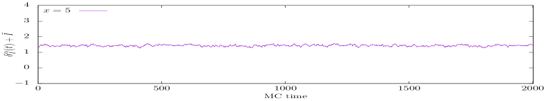
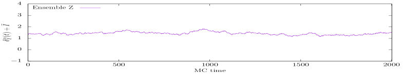
Figure 4: Fluctuations for the observable $I$ over the mean ($\delta_{I}^{\alpha}(t)+\bar{I}$) (see equation (2.22)) corresponding to each ensemble that contributes to its error ($\alpha=x_{i},Z$). Despite fluctations being small in amplitude, ensemble $Z$ contributes a 61% to the error in $I$ (the largest contribution).

5.1 Exact error propagation

In order to support our claim that AD techniques perform linear propagation of errors exactly, it is interesting to compare the result of the procedure described in section 4.2 (based on computing the Hessian at the minimum) with an implementation of the fitting procedure where all operations are performed in the hyper-dual field. For this last case we use a simple (and inefficient) minimizer: a simple gradient descent with a very small and constant damping parameter. We point out that our inefficient algorithm needs $\mathcal{O}(2000)$ iterations of the loop in algorithm 1 to converge to the solution.

Since each operation in the algorithm is performed in the hyper-dual field we are exactly evaluating the derivative of the fitting routine with respect to the data points that enter in the evaluation of the $\chi^{2}$. These derivatives are all that is needed to perform linear error propagation. All derivatives are computed to machine precision.

Being more explicit, if we define a function that performs one iteration of the gradient descent (see algorithm 1)

$$\mathbf{\mathcal{I}}(\mathbf{x})=\mathbf{x}-\gamma\mathbf{\nabla}\chi^{2}\Big{|}_{\mathbf{x}}\,,$$ (5.5)

we can define the function

$$\mathcal{M}=\underbrace{\mathcal{I}\circ\mathcal{I}\circ\cdots\circ\mathcal{I}}_{\text{2000 times!}}\,,$$ (5.6)

that returns the minima of the $\chi^{2}$ for any reasonable input. AD is computing the derivative of $\mathcal{M}$ with respect to the data that enter the evaluation of the $\chi^{2}$ exactly.

On the other hand the derivation of section 4.2 is also exact to leading order. Therefore both procedures should give the same errors, even if in one case we are computing the derivative just by making the derivative of every operation of the gradient descent algorithm, and in the other case we are exactly computing the Hessian of the $\chi^{2}$ function at the minima and using it for linear error propagation. The results of this small test confirm our expectations:

$$\textbf{Gradient:}\quad n=0.97959028626531608 \pm 0.193130534135\,80400\,.$$ (5.7)

$$\textbf{Hessian:}\quad n=0.97959028626531608 \pm 0.193130534135\,94974\,.$$ (5.8)

$$\textbf{Gradient:}\quad m=0.36501862665927676 \pm 4.4699145709\,887811\times 10^{-2}\,.$$ (5.9)

$$\textbf{Hessian:}\quad m=0.36501862665927676 \pm 4.4699145709\,956804\times 10^{-2}\,.$$ (5.10)

As the reader can see both errors agree with more than 12 decimal places. The critical reader can still argue that in fact the errors are not exactly the same. One might be tempted to say that the small difference is due to “higher orders terms” in the expansion performed in section 4.2, but this would be wrong (AD is an exact truncation up to some order). The reason of the difference are “lower order terms”. In the derivation of section 4.2 we have assumed that the $\chi^{2}$ is in the minimum. In fact, any minimization algorithm returns the minimum only up to some precision. This small deviation from the true minimum gives a residual gradient of the $\chi^{2}$ function that contaminates (the 14${}^{\underline{th}}$ significant digit!) of the errors in the fit parameters.

Algorithm 1 Gradient descent

1:$\gamma\leftarrow 0.0001$

2:$X_{i}^{(1)}\leftarrow 1.0$

3:$\epsilon\leftarrow 10^{-12}$

4:repeat

5:     $X_{i}^{(0)}\leftarrow X_{i}^{(1)}$

6:     $df_{i}\leftarrow{\partial\chi^{2}}/{\partial x_{i}}$

7:     $X_{i}^{(1)}\leftarrow X_{i}^{(0)}-\gamma*df_{i}$

8:until ($|df|<\epsilon)\,\textbf{and}\,(|X^{(1)}-X^{(0)}|<\epsilon)$

6 Conclusions

Lattice QCD is in a precision era. Input from lattice QCD is used to challenge the Standard Model in several key areas like flavor physics, CP violation or the anomalous moment of the muon to mention a few examples. It is very likely that if new physics is discovered in the next ten years, lattice QCD will be used as input. Error analysis of lattice data is a key ingredient in the task of providing this valuable input to the community.

The state of the art lattice simulations that provide this important input to the particle physics community require simulations at small lattice spacings and large physical volumes. It is well-known that these simulations in general (and specially if topology freezing [14] plays a role) have large exponential autocorrelation times. The field continues to push their simulations to smaller and smaller lattice spacings to be able to simulate relativistic charm and bottom quarks comfortably, making the issue of large autocorrelation times more severe.

There are good theoretical and practical reasons to use the $\Gamma$-method as tool for data analysis. Despite these arguments are known for more than ten years (see [1]), most of the treatment of autocorrelations in current state of the art computations use binning techniques, known to underestimate the errors, specially in the current situation of large autocorrelations. There are known solutions to these issues: the $\Gamma$-method [2, 1, 3] allows to study in detail the autocorrelations even of complicated derived observables, and to include in the error estimates the effect of the slow modes of the MC chain. The author does not know any other analysis technique that allow to estimate statistical uncertainties conservatively at the simulation parameters of current state of the art lattice QCD simulations.

In this work we have considered the analysis of general observables that depend on several MC simulations with the $\Gamma$-method. We have shown that linear error propagation can be performed exactly, even in arbitrarily complicated observables defined via iterative algorithms. Thanks to automatic differentiation we only need to extend the operations and evaluation of intrinsic fundamental functions to the field of hyper-dual numbers. Moreover error propagation in certain iterative procedures can be significantly simplified. In particular we have examined in detail the interesting case of fitting some Monte Carlo data and the case of error propagation in the determination of the root of a non-linear function. We have shown that error propagation in these cases only require to use AD once the fit parameters or the root of the function are known. Conveniently, AD techniques are not needed in the fitting or root finding algorithms and one can rely on external libraries to perform these tasks. By comparing these techniques with an implementation of a fitting algorithm where all operations are performed in the hyper-dual field we have explicitly checked that error propagation is performed exactly. In summary, AD techniques in conjunction with the $\Gamma$-method offer a flexible approach to error propagation in general observables.

Analysis of Monte Carlo data along the lines proposed in this work is robust in the sense that if in any analysis the central values of the parameters are computed correctly, the exact nature of the truncation performed in AD guarantees that errors will be correctly propagated. Although the focus in this work has been on the applications of AD to analysis of Lattice QCD data, the ideas described here might find its way to other research areas.

Implementing the $\Gamma$-method for data analysis is usually cumbersome: different MC chains have to be treated independently and an efficient computation of the autocorrelation functions requires to use the Fast Fourier Transform. We provide a portable, freely available implementation of an analysis code that handles the analysis of observables derived from measurements on any number of ensembles and any number of replicas. Error propagation, even in iterative algorithms, is exact thanks to AD [10]. We hope that future analysis in the field can either use it directly, or as a reference implementation for other robust and efficient analysis tools of MC data.

Appendix A A model to study analysis of autocorrelated data

In algorithms with detailed balance the autocorrelation function of any observable can be written as a sum of decaying exponential

$$\Gamma(t)=\sum_{k}\zeta_{k}e^{-|t|/\tau_{k}}\,,\qquad(\zeta_{k}>0)\,,$$ (A.1)

where the $\tau_{k}$ are related with the left eigenvectors of the Markov operator. They are universal in the sense that they are a property of the algorithm. Different observables decay with the same values $\tau_{k}$. On the other hand the “couplings” $\zeta_{k}$ are observable dependent.

As proposed in [1] one can simulate noisy autocorrelated data using Gaussian independent random numbers

$$\eta(t)\sim\mathcal{N}(0,1)\,,$$ (A.2)

just defining

$$\nu^{(k)}(t)=\sqrt{1-e^{-2/\tau_{k}}}\,\eta(t)+e^{-1/\tau_{k}}\nu(t-1)\,.$$ (A.3)

The autocorrelation function for the variable $\nu^{(k)}(t)$ is trivially computed to be $e^{-|t|/\tau_{k}}$. One can now construct a linear combination of such variables

$$x(t)=x_{\rm mean}+\sum_{k}\lambda_{k}\nu^{(k)}(t)\,,$$ (A.4)

that has an autocorrelation function of the type equation (A.1). A straightforward computation yields

$$\Gamma_{x}(t) = \langle x(0)x(t)\rangle=\sum_{k}\lambda_{k}^{2}e^{-|t|/\tau_{k}}\,,\qquad\left(\Gamma_{x}(0)=\sum_{k}\lambda_{k}^{2}\right)\,.$$ (A.5)

$$\rho_{x}(t) = \sum_{k}\frac{\lambda_{k}^{2}}{\Gamma_{x}(0)}e^{-|t|/\tau_{k}}\,.$$ (A.6)

$$\tau_{{\rm int},x} = \frac{1}{2}+\sum_{t=1}^{\infty}\rho_{x}(t)=\frac{1}{2}+\sum_{k}\frac{\lambda_{k}^{2}}{\Gamma_{x}(0)(e^{1/\tau_{k}}-1)}\,.$$ (A.7)

Finally the error for a sample of length $N$ is

$$(\delta x)^{2}=\frac{1}{N}\left(\Gamma_{x}(0)+2\sum_{k}\frac{\lambda_{k}^{2}}{e^{1/\tau_{k}}-1}\right)\,.$$ (A.8)

And if we decide to truncate the infinite sum in eq. (A.7) with a window of size $W$, we get

$$(\delta_{W}x)^{2}=\frac{1}{N}\left(\Gamma_{x}(0)+2\sum_{k}\frac{\lambda_{k}^{2}(1-e^{-W/\tau_{k}})}{e^{1/\tau_{k}}-1}\right)\,.$$ (A.9)

Adding the tail with the slowest mode $\tau_{\rm exp}=\max\{\tau_{k}\}$ after summing the autocorrelation function up to $W$ gives as result

$$(\delta_{\rm exp}x)^{2}=\frac{1}{N}\left(\Gamma_{x}(0)+2\sum_{k}\frac{\lambda_{k}^{2}(1-e^{-W/\tau_{k}})}{e^{1/\tau_{k}}-1}+2\tau_{\rm exp}e^{-(W+1)/\tau_{\rm exp}}\sum_{k}\lambda_{k}^{2}\right)\,.$$ (A.10)

A.1 Binning

Binning can also be studied exactly in this model. Bins of length $N_{B}$ are defined by block averaging

$$b(\alpha)=\frac{1}{N_{B}}\sum_{i=1}^{N_{B}}x((\alpha-1)N_{B}+i)\,.$$ (A.11)

The autocorrelation function of the binned data is given by

$$\Gamma_{b}(t) = \langle b(\alpha+t)b(\alpha)\rangle=\frac{1}{N_{B}^{2}}\sum_{i,j=1}^{N_{B}}\Gamma_{x}(tN_{B}+i-j)$$ (A.12)

$$= \frac{1-\delta_{t,0}}{N^{2}_{B}}\sum_{k}\lambda_{k}^{2}K(N_{B},\tau_{k})+\frac{\delta_{t,0}}{N^{2}_{B}}\sum_{k}\lambda_{k}^{2}H(N_{B},\tau_{k})\,,$$ (A.13)

where the functions $K(N,\tau)$ and $H(N,\tau)$ are given by

$$K(N,\tau) = \frac{1-\cosh(N/\tau)}{1-\cosh(1/\tau)}\,,$$ (A.14)

$$H(N,\tau) = N\left[1+2e^{-1/\tau}\frac{1-e^{-(N-1)/\tau}}{1-e^{-1/\tau}}\right]$$

$$- 2e^{-1/\tau}\frac{1-Ne^{-(N-1)/\tau}+(N-1)e^{-N/\tau}}{(1-e^{-1/\tau})^{2}}\,.$$

Now we can determine the normalized autocorrelation function and the integrated autocorrelation time of the binned data

$$\Delta = \sum_{k}\lambda_{k}^{2}H(N_{B},\tau_{k})\,,$$ (A.16)

$$\rho_{b}(t) = \Delta^{-1}\sum_{k}\lambda_{k}^{2}K(N_{B},\tau_{k})e^{-tN_{B}/\tau_{k}}\,,\qquad(t>0)\,.$$ (A.17)

$$\tau_{{\rm int},b} = \frac{1}{2}+\Delta^{-1}\sum_{k}\lambda_{k}^{2}\frac{K(N_{B},\tau_{k})}{e^{N_{B}/\tau_{k}}-1}\,.$$ (A.18)

Resampling techniques (bootstrap, jackknife) treat the bins as independent variables. Therefore the error estimate for a sample of length $N$ is

$$(\delta_{\rm binning}x)^{2}=\frac{\Delta}{NN_{B}^{2}}\,,$$ (A.19)

while the true error eq. (A.8) can conveniently be written as

$$(\delta x)^{2}=\frac{1}{NN_{B}^{2}}\left(\Delta+2\sum_{k}\lambda_{k}^{2}\frac{K(N_{B},\tau_{k})}{e^{N_{B}/\tau_{k}}-1}\right)\,,$$ (A.20)

Appendix B A free implementation of the $\Gamma$-method with AD error propagation

Here we present a freely available fortran 2008 library for data analysis using the $\Gamma$-method with AD for linear error propagation. The software is standard compliant and have no external dependencies beyond a fortran compiler that supports the modern standards. The code can handle the analysis of several replica and observables from different ensembles. For a detailed documentation and to obtain a copy of the software check [10].

B.1 A complete example

This is a complete commented example that shows most of the features of the code. This particular snippet is part of the distribution [10] (file test/complete.f90 (see B.1.1)). It uses the module simulator (test/simulator.f90) that generates autocorrelated data along the lines of appendix A. Here we give an overview on the package using a full example where we compute the error in the derived quantity

$$z=\frac{\sin x}{\cos y+1}\,.$$ (B.1)

The quantities $x$ and $y$ are generated using the procedure described in appendix A and are assumed to originate from simulations with completely different parameters. The line numbers correspond to the listing in section B.1.1.

lines 4-7

modules provided with the distribution [10].

lines 21-36

Use module simulator to produce measurements for two observables from different ensembles. On the first MC ensemble we have $\tau_{k}=[1.0,3.0,12.0,75.0]$ and the measurements data_x(:) correspond to couplings $\lambda_{k}=[1.0,0.70,0.40,0.40]$. For the second MC ensemble we have $\tau_{k}=[2.0,4.0,6.0,8.0]$ and the measurements data_y(:) have couplings $\lambda_{k}=[2.3,0.40,0.20,0.90]$. In the first case we have a sample of length 5000 in 4 replicas of sizes $1000,30,3070,900$. For the second MC chain we have a single replica of size 2500. See appendix A for analytic expressions of the error of both observables.

lines 42-45

Load measurements of the first observable in the variable x, and set the details of the analysis:

line 43

Set the ensemble ID to 1.

line 44

Set replica vector to $[1000,30,3070,900]$.

line 45

Set the exponential autocorrelation time ($\tau_{\rm exp}=75$).

lines 48-49

Load measurements of the second ensemble into y and set ensemble ID to 2. In this case we have only one replica (the default), and we choose not to add a tail to the autocorrelation function since the number of measurements (2500) is much larger than the exponential autocorrelation time $\tau_{\rm exp}=8$ of the second MC ensemble.

line 52

Computes the derived observable z.

lines 56-58

Details of the analysis for observable z:

line 56

Add the tail to the normalized autocorrelation function at the point where the signal $\rho(t)$ is equal to 1.0 times the error and the ensemble ID is 1.

line 58

Set the parameter $S_{\tau}=3$ for ensemble ID 2 to automatically choose the optimal window (see [1]).

line 60

Performs the error analysis in z.

lines 62-68

Prints estimate of the derived observable with the error. Also prints $\tau_{\rm int}$ for each ensemble and what portion of the final error in z comes from each ensemble ID.

lines 70-72

Prints in file history_z.log the details of the analysis: fluctuations per ensemble, normalized autocorrelation function and $\tau_{\rm int}$ as a function of the Window size. This allows to produce the plots in Fig. 5.

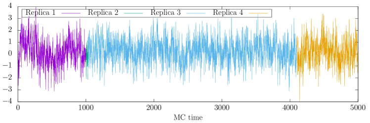
(a) MC history for ID 1

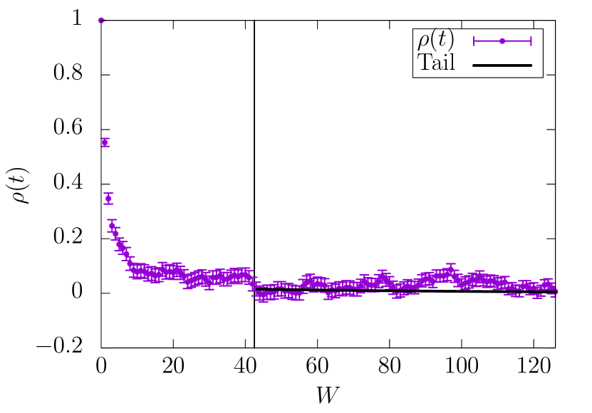
(b) Normalized autocorrelation function for ID 1

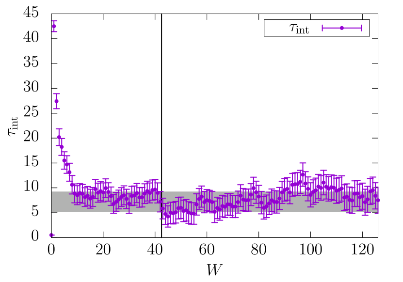
(c) $\tau_{\rm int}$ for ID 1

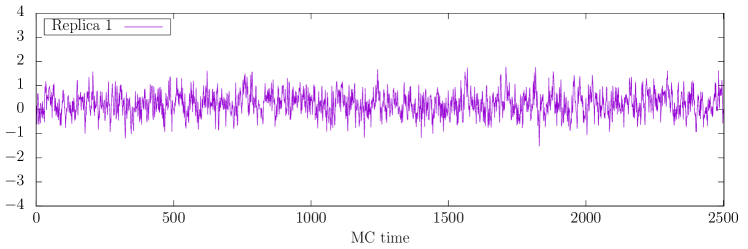
(d) MC history for ID 2

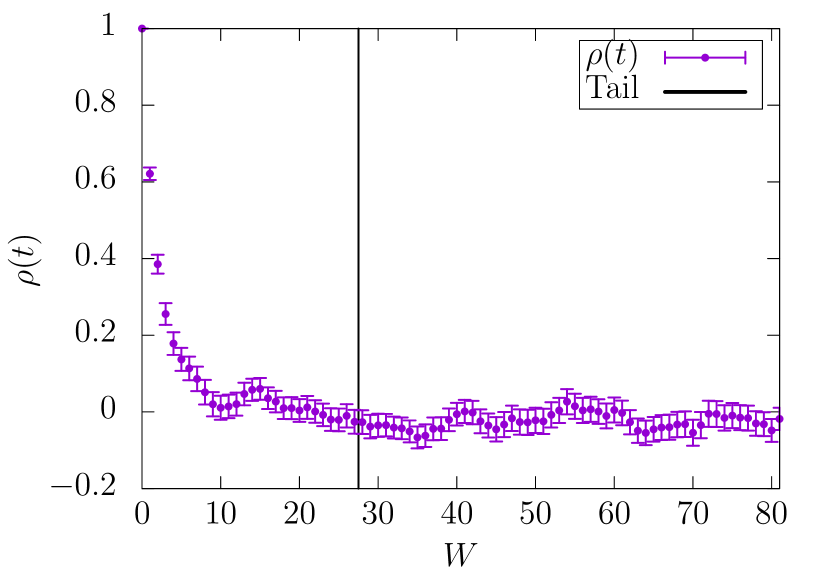
(e) Normalized autocorrelation function for ID 2

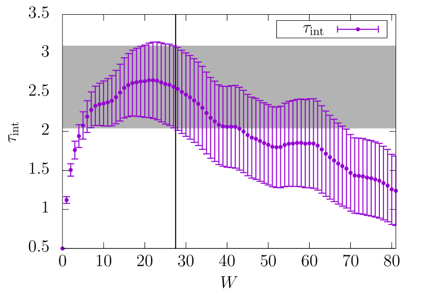
(f) $\tau_{\rm int}$ for ID 2

Figure 5: Histories, autocorrelation functions and $\tau_{\rm int}$ for the derived observable $z$ (eq. (B.1)).

Running the code produces the output

 Observable z:     0.24426076465139626       +/-    5.8791563778643217E-002
   Contribution to error from ensemble ID  1   86.57%  (tau int: 7.2020 +/-   2.0520)
   Contribution to error from ensemble ID  2   13.43%  (tau int: 2.5724 +/-   0.5268)

B.1.1 Example code listing

⬇

1program complete

2

3 use ISO_FORTRAN_ENV, Only : error_unit, output_unit

4 use numtypes

5 use constants

6 use aderrors

7 use simulator

8

9 implicit none

10

11 integer, parameter :: nd = 5000, nrep=4

12 type (uwreal) :: x, y, z

13 integer :: iflog, ivrep(nrep)=(/1000,30,3070,900/), i, is, ie

14 real (kind=DP) :: data_x(nd), data_y(nd/2), err, ti, texp

15 real (kind=DP) :: tau(4), &

16 lam_x(4)=(/1.0_DP, 0.70_DP, 0.40_DP, 0.40_DP/), &

17 lam_y(4)=(/2.3_DP, 0.40_DP, 0.20_DP, 0.90_DP/)

18 character (len=200) :: flog=’history_z.log’

19

20

21 ! Fill arrays data_x(:) with autocorrelated

22 ! data from the module simulator. Use nrep replica

23 tau = (/1.0_DP, 3.0_DP, 12.0_DP, 75.0_DP/)

24 texp = maxval(tau)

25

26 is = 1

27 do i = 1, nrep

28 ie = is + ivrep(i) - 1

29 call gen_series(data_x(is:ie), err, ti, tau, lam_x, 0.3_DP)

30 is = ie + 1

31 end do

32

33 ! Fill data_y(:) with different values of tau also using

34 ! module simulator

35 forall (i=1:4) tau(i) = real(2*i,kind=DP)

36 call gen_series(data_y, err, ti, tau, lam_y, 1.3_DP)

37

38

39 ! Load data_x(:) measurements in variable x.

40 ! Set replica vector, exponential autocorrelation time

41 ! and ensemble ID.

42 x = data_x

43 call x%set_id(1)

44 call x%set_replica(ivrep)

45 call x%set_texp(texp)

46

47 ! Load data_y(:) measurements in variable y

48 y = data_y

49 call y%set_id(2)

50

51 ! Exact, transparent error propagation

52 z = sin(x)/(cos(y) + 1.0_DP)

53

54 ! Attach tail in ensemble with ID 1 when signal in the

55 ! normalized auto-correlation function equals its error

56 call z%set_dsig(1.0_DP,1)

57 ! Set Stau=3 for automatic window in ensemble with ID 2

58 call z%set_stau(3.0_DP,2)

59 ! Perform error analysis (tails, optimal window,...)

60 call z%uwerr()

61

62 ! Print results and output details to flog

63 write(*,’(1A,1F8.5,1A,1F8.5)’)’** Observable z: ’, z%value(), " +/- ", z%error()

64 do i = 1, z%neid()

65 write(*,’(3X,1A,1I3,3X,1F5.2,"%")’,advance="no")’Contribution to error from ensemble ID’, &

66 z%eid(i), 100.0_DP*z%error_src(i)

67 write(*,’(2X,1A,1F0.4,1A,1F8.4,1A)’)’(tau int: ’, z%taui(i), " +/- ", z%dtaui(i), ")"

68 end do

69

70 open(newunit=iflog, file=trim(flog))

71 call z%print_hist(iflog)

72 close(iflog)

73

74 stop

75end program complete

References

- [1] ALPHA Collaboration, U. Wolff, “Monte Carlo errors with less errors,” Comput.Phys.Commun. 156 (2004) 143–153, arXiv:hep-lat/0306017 [hep-lat].
- [2] N. Madras and A. D. Sokal, “The pivot algorithm: A highly efficient monte carlo method for the self-avoiding walk,” Journal of Statistical Physics 50 no. 1, (Jan, 1988) 109–186. https://doi.org/10.1007/BF01022990.
- [3] ALPHA Collaboration, S. Schaefer, R. Sommer, and F. Virotta, “Critical slowing down and error analysis in lattice QCD simulations,” Nucl. Phys. B845 (2011) 93–119, arXiv:1009.5228 [hep-lat].
- [4] Wikipedia contributors, “Automatic differentiation — Wikipedia, the free encyclopedia,” 2018. https://en.wikipedia.org/wiki/Automatic_differentiation. [Online; accessed 22-June-2018].
- [5] F. Virotta, Critical slowing down and error analysis of lattice QCD simulations. PhD thesis, Humboldt-Universität zu Berlin, Mathematisch-Naturwissenschaftliche Fakultät I, 2012.
- [6] Lottini, S. and Sommer, R., “Data analysis – lattice practices,” 2014. https://indico.desy.de/indico/event/9420/. Theory and Practice of data analysis.
- [7] Hubert Simma and Rainer Sommer and Francesco Virotta, “General error computation in lattice gauge theory,” 2012-2014. Internal notes ALPHA collaboration.
- [8] Lebigot, Eric O., “Uncertainties: a python package for calculations with uncertainties,” 2018. http://pythonhosted.org/uncertainties/. Uncertainties in python.
- [9] B. De Palma, M. Erba, L. Mantovani, and N. Mosco, “A Python program for the implementation of the -method for Monte Carlo simulations,” arXiv:1703.02766 [hep-lat].
- [10] Ramos, Alberto, “aderrors: Error analysis of monte carlo data with automatic differentiation,” 2018. https://gitlab.ift.uam-csic.es/alberto/aderrors.
- [11] S. Linnainmaa, “Taylor expansion of the accumulated rounding error,” BIT Numerical Mathematics 16(2) (1976) 146–160.
- [12] A. Griewank, Evaluating derivatives : principles and techniques of algorithmic differentiation. Society for Industrial and Applied Mathematics, Philadelphia, PA, 2008.
- [13] J. A. Fike and J. J. Alonso, “The development of hyper-dual numbers for exact second-derivative calculations,” in AIAA paper 2011-886, 49th AIAA Aerospace Sciences Meeting. 2011.
- [14] L. Del Debbio, G. M. Manca, and E. Vicari, “Critical slowing down of topological modes,” Phys.Lett. B594 (2004) 315–323, arXiv:hep-lat/0403001 [hep-lat].