KMT-2017-BLG-0165Lb: A Super-Neptune mass planet Orbiting a Sun-like Host Star

Abstract

We report the discovery of a low mass-ratio planet $(q=1.3\times 10^{-4})$, i.e., 2.5 times higher than the Neptune/Sun ratio. The planetary system was discovered from the analysis of the KMT-2017-BLG-0165 microlensing event, which has an obvious short-term deviation from the underlying light curve produced by the host of the planet. Although the fit improvement with the microlens parallax effect is relatively low, one component of the parallax vector is strongly constrained from the light curve, making it possible to narrow down the uncertainties of the lens physical properties. A Bayesian analysis yields that the planet has a super-Neptune mass $(M_{2}=34_{-12}^{+15}~{}M_{\oplus})$ orbiting a Sun-like star $(M_{1}=0.76_{-0.27}^{+0.34}~{}M_{\odot})$ located at $4.5~{}{\rm kpc}$. The blended light is consistent with these host properties. The projected planet-host separation is $a_{\bot}={3.45_{-0.95}^{+0.98}}~{}{\rm AU}$, implying that the planet is located outside the snowline of the host, i.e., $a_{sl}\sim 2.1~{}{\rm AU}$. KMT-2017-BLG-0165Lb is the sixteenth microlensing planet with mass ratio $q<3\times 10^{-4}$. Using the fifteen of these planets with unambiguous mass-ratio measurements, we apply a likelihood analysis to investigate the form of the mass-ratio function in this regime. If we adopt a broken power law for the form of this function, then the break is at $q_{\rm br}\simeq 0.55\times 10^{-4}$, which is much lower than previously estimated. Moreover, the change of the power law slope, $\zeta>3.3$ is quite severe. Alternatively, the distribution is also suggestive of a “pile-up” of planets at Neptune-like mass ratios, below which there is a dramatic drop in frequency.

1 Introduction

Up to now, there have been many discoveries of planets via various detection methods, which are currently reaching about 4000 planets according to the NASA Exoplanet Archive . Most of these planets were discovered and characterized by the transit (e.g., Tenenbaum et al. 2014) and radial-velocity (e.g., Pepe et al. 2011) methods. These methods favor the detection of close-in planets around their hosts stars, and the majority of the hosts are Sun-like stars located in the solar neighborhood.

On the other hand, the microlensing method favors the detection of planets down to one Earth mass orbiting outside the snow line, where the temperature is cool enough for icy material to condense (Ida & Lin, 2004). Instead of looking for light from the host stars, microlensing uses the light of a background source refracted by the gravitational potential of an aligned foreground planetary system. This allows the method to detect planets around all types of stellar objects at Galactocentric distances and even free-floating planets, which may have been ejected from their host stars (Sumi et al., 2011; Mróz et al., 2017b, 2018). Hence, although the number of planets discovered by microlensing is relatively small ($\sim 60$ discoveries to date), the method can access a class of planets that are inaccessible to other detection methods, and help to expand our understanding of planet populations.

Based on microlensing planets, statistical works have been conducted to examine the properties of planets beyond the snow line. As presented in Mróz et al. (2017a), microlensing planets are nearly uniformly distributed in ${\rm log}~{}q$, where $q=M_{2}/M_{1}$ is the planet/host mass ratio. Because the probability for detecting planets increases with $q$, this implies that the planet frequency has a rising shape toward lower mass ratios. Sumi et al. (2010) investigated this distribution and found that the frequency can be described by a single power-law mass-ratio function, i.e., $dN/d{\rm log}~{}q\propto q^{n}$, where $n$ is the power-law index. However, Suzuki et al. (2016) argued that there exists a break in the power-law function at $q_{\rm br}\simeq 1.7\times 10^{-4}$. They found that the planet frequency rises rapidly toward lower mass ratios above the break, but falls off just as rapidly toward lower mass ratios below the break. Udalski et al. (2018) confirmed this turnover by refining the power-law index using seven microlensing planets in the $q<10^{-4}$ regime. This broken power law would imply that the planet/host mass ratio provides a strong constraint to planet formation beyond the snow line. Furthermore, considering that the mass ratio at the break corresponds to $\sim 20~{}M_{\oplus}$ for the median host mass of $0.6~{}M_{\odot}$, it also would suggest that Neptune-mass planets are the most common population of planets outside the snow line (Gould et al., 2006). However, the precise mass ratio at the break remains uncertain, and the nature of the rapid descent below the break is barely probed due to the insufficient sample in this regime. Hence, discovering microlensing planets whose mass ratios are located near or below the break is important to improve our understanding of planet abundances.

In this paper, we report the discovery of a super-Neptune mass planet hosted by a Sun-like star, i.e., with a mass ratio close to $q_{\rm br}$ as found by Suzuki et al. (2016). The planetary system was identified from the analysis of microlensing event KMT-2017-BLG-0165, which has an obvious short-term deviation from its underlying single-lens light curve (Paczyński, 1986). Despite the short duration, the deviation was clearly detected from the Korea Microlensing Telescope Network (KMTNet: Kim et al., 2016) high-cadence microlensing survey. We also investigate the value of $q_{\rm br}$ in more detail.

2 Observation

The lensing event KMT-2017-BLG-0165 occurred on a star located at $({\rm RA},{\rm Dec})_{\rm J2000}=$(17:58:35.92, $-28$:08:01.21) or $(l,b)=(2.14,-2.04)$ in Galactic coordinates. It was found by applying the KMTNet event-finder algorithm (Kim et al., 2018) to the 2017 KMTNet survey data from three 1.6 m telescopes distributed over three different sites, i.e., the Cerro Tololo Inter-American Observatory in Chile (KMTC), the South African Astronomical Observatory in South Africa (KMTS), and the Siding Spring Observatory in Australia (KMTA). The event is located in four overlapping fields (BLG02, BLG03, BLG42, and BLG43), monitored with a combined cadence of $8~{}{\rm hr}^{-1}$. KMTNet images were obtained primarily in $I$ band, while some $V$-band images were obtained solely to secure the colors of the source stars. All data for the light curve analysis were reduced using the pySIS method (Albrow et al., 2009), a variant of difference image analysis (DIA: Alard & Lupton, 1998).

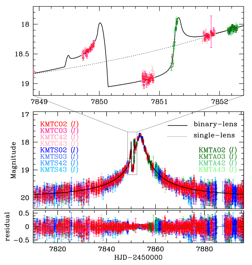
Figure 1: Light curve of KMT-2017-BLG-0165. The upper panel shows the zoom of the planetary perturbation centered at ${\rm HJD}^{\prime}\sim 7850.6$. The black curve is the model derived from the binary-lens interpretation, whereas the dotted grey curve is derived from the single-lens interpretation.

Figure 1 shows the light curve of KMT-2017-BLG-0165. Except for a deviation during the interval $7849<{\rm HJD}^{\prime}(={\rm HJD}-2450000)<7852$, the overall shape of the light curve resembles a standard single-lens curve with a moderate magnification $A_{\rm max}\sim 32$ at the peak. The most prominent feature of the deviation is a trough lying about 0.4 mag below the level of the single-lens curve. This trough is a characteristic feature of lensing systems with planet-host separations $s<1$ (in units of the angular Einstein radius, $\theta_{\rm E}$) and small mass ratios $q\ll 1$, i.e., planetary systems. In the underlying microlensing event, the host of a planet will split the source light into two magnified images, one inside (minor) and the other outside (major) the Einstein ring. Because the former image is highly unstable, it will be easily suppressed if the planet lies in or near the path of the image, thereby causing a trough in the light curve (Gaudi, 2012). Such troughs are always flanked by two triangular caustics centered on the host-planet axis. If the source passes very close to or over these caustics, the light curve would exhibit sharp breaks near the trough. Hence, from the form of the deviation at ${\rm HJD}^{\prime}\sim 7851.2$, it is suggested that there exists an interaction between the source and the triangular caustics.

3 Analysis

Considering that the light curve appears to be a planetary event, we model the event with the binary-lens interpretation. For a standard binary-lens model, one needs seven fitting parameters. Three of these parameters $(t_{0},u_{0},t_{\rm E})$ describe the source approach relative to the lens, and their definitions are the same as those for the Paczyński (1986) curve, i.e., the moment of closet approach, the impact parameter (in unit of $\theta_{\rm E}$), and the Einstein timescale. Another three parameters $(s,q,\alpha)$ describe the binary lens companion. As already described, $s$ and $q$ are the normalized separation and the mass ratio, whereas $\alpha$ is the angle of the source trajectory relative to the binary axis. The last parameter, $\rho_{*}$, is the source radius $\theta_{*}$ in units of $\theta_{\rm E}$.

For the case that planetary deviations can be regarded as perturbations, the light curve except the deviations follows the underlying standard single-lens curve. The fitting parameters can then be estimated heuristically from the location and duration of the deviation (Gould & Loeb, 1992). By excluding the perturbation in the light curve, we find that the single-lens fit yields $(t_{0},u_{0},t_{\rm E})=(7853.70,0.035,42.03~{}{\rm days})$, which corresponds to an effective timescale of $t_{\rm eff}\equiv u_{0}t_{\rm E}=1.47~{}{\rm days}$. The perturbation is centered at ${\delta}t=3.2$ days before the peak, implying that the trajectory angle is $\alpha={\rm tan}^{-1}(t_{\rm eff}/{\delta}t)=5.85$ rad. The normalized separation $s$ is then estimated by

$$s-{1\over s}=u_{0}\sqrt{1+\left({{\delta}t\over t_{\rm eff}}\right)^{2}},$$ (1)

which indicates $s=0.96$. Note that we exclude the other $(s>1)$ solution because it would produce a positive deviation. The mass ratio $q$ is related to the duration of the trough ${\Delta}t$ and the separation by

$$q={\eta_{c,-}^{2}\over 4(s^{2}-1)};~{}~{}~{}~{}~{}{\Delta}t=2t_{\rm E}\eta_{c,-}|{\rm sec}~{}\alpha|,$$ (2)

where $\eta_{c,-}$ is the vertical position of triangular-caustic-fold facing the trough (Han, 2006). From the light curve, we estimate ${\Delta}t\sim 0.8~{}{\rm days}$. Hence, the mass ratio is $q\sim 2.2\times 10^{-4}$.

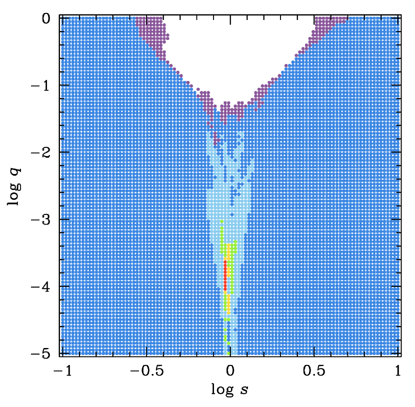
Figure 2: $\Delta\chi^{2}$ surface in $({\rm log}~{}s,{\rm log}~{}q)$ plane drawn from the grid search. The plane is color coded by $\Delta\chi^{2}$ $<(1\,n)^{2}$ (red), $<(2\,n)^{2}$ (yellow), $<(3\,n)^{2}$ (green), $<(4\,n)^{2}$ (light blue), $<(5\,n)^{2}$ (blue), and $<(6\,n)^{2}$ (purple) level from the initial best-fit solution, where $n=20$.

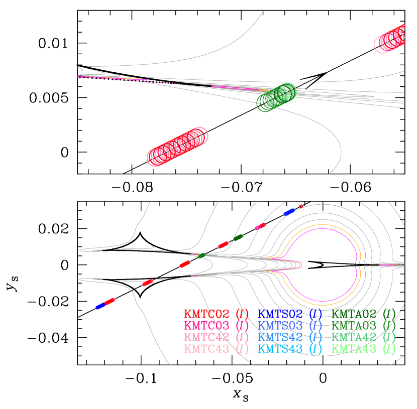
Figure 3: Caustic structure of KMT-2017-BLG-0165. The source passes over the trough flanked by the two triangular caustics, resulting from the minor image perturbation. The upper panel shows the zoom of the triangular caustic at the time of the source’s cusp approach. The open circles represent the source location at the times of observation, and their size is scaled by the source radius $\rho_{*}$ of the best-fit solution. The grey curves are the magnification contours of $A=(10,15,20,25,30,35,40)$, while the yellow and magenta curves are the contours of $A=45$ and $50$, respectively.

For precise measurements of the fitting parameters, we conduct a systematic analysis by adopting the method of Jung et al. (2015). First, we perform a grid search over $(s,q,\alpha)$ space, in which we fit the light curve using a downhill approach with a Markov Chain Monte Carlo (MCMC) algorithm. At each data point, we compute the magnification using inverse ray-shooting (Kayser et al., 1986; Schneider & Weiss, 1987) in the neighboring region around caustics and the semi-analytic multipole approximation (Pejcha & Heyrovský, 2009; Gould, 2008) elsewhere. Next, we investigate the local $\chi^{2}$ minima from the derived $\Delta\chi^{2}$ map in the $({\rm log}~{}s,~{}{\rm log}~{}q)$ space. From this, we find only one local minimum, which has a separation that is slightly lower than unity and a mass ratio that is in the range of $0.8\times 10^{-4}<q<3\times 10^{-4}$. These are very close to the predictions from the heuristic analysis (see Figure 2). To find the global solution, we then explore the local solution by optimizing all fitting parameters. The best-fit standard parameters are given in Table 1. In Figure 1, we present the model curve superposed on the data. The corresponding caustic structure is shown in Figure 3.

For some binary-lens events, the observed light curve can exhibit further deviations from the form expected from the standard model. This often occurs in long-timescale events for which the approximation that the source motion relative to the lens is rectilinear is no longer valid. There are two major effects that can cause such deviations, i.e., “microlens-parallax” and “lens-orbital” effects. The former is caused by the orbital acceleration of Earth (Gould, 1992), while the latter is caused by the orbital acceleration of the lens (Dominik, 1998; Jung et al., 2013). The parallax effect is described by two parameters $\mbox{\boldmath$\pi$}_{\rm E}=(\pi_{{\rm E},N},\pi_{{\rm E},E})$, which are the components of parallax vector, i.e.,

$$\mbox{\boldmath$\pi$}_{\rm E}\equiv\pi_{\rm E}{\mbox{\boldmath$\mu$}_{\rm geo}\over\mu_{\rm geo}};~{}~{}~{}~{}~{}\pi_{\rm E}={\pi_{\rm rel}\over\theta_{\rm E}},$$ (3)

where $\pi_{\rm rel}={\rm AU}(D_{\rm L}^{-1}-D_{\rm S}^{-1})$ is the relative lens-source parallax, and $D_{\rm L}$ and $D_{\rm S}$ are, respectively, the lens and source distances. Here $\mbox{\boldmath$\mu$}_{\rm geo}$ is the geocentric lens-source relative proper motion. The lens-orbital effect is described by two linearized parameters $\bm{\gamma}=[(ds/dt)/s,d\alpha/dt]$, which denote the instantaneous time derivatives of $\ln s$ and $\alpha$, respectively. These orbit parameters can be correlated with $\mbox{\boldmath$\pi$}_{\rm E}$, and thus they also should be included when incorporating the parallax parameters into the analysis (Batista et al., 2011; Skowron et al., 2011; Han et al., 2016). We note that if one has an estimate for both $\pi_{\rm E}$ and $\theta_{\rm E}$, the physical lens parameters (lens mass $M_{\rm tot}$ and $D_{\rm L}$) can be determined by

$$M_{\rm tot}={\theta_{\rm E}\over\kappa\pi_{\rm E}};~{}~{}~{}~{}~{}D_{\rm L}={{\rm AU}\over\pi_{\rm E}\theta_{\rm E}+\pi_{\rm S}},$$ (4)

where $\kappa=4G/(c^{2}{\rm AU})\sim 8.14~{}{\rm mas}~{}M_{\odot}^{-1}$ and $\pi_{\rm S}={\rm AU}/D_{\rm S}$.

The duration of the event is $t_{\rm d}=2(1-u_{0}^{2})^{1/2}t_{\rm E}\sim 85~{}{\rm days}$, which covers a significant portion of Earth’s orbit period. Hence, we additionally fit the light curve by introducing the above higher-order parameters to the standard model. In this modeling, we also test $u_{0}>0$ and $u_{0}<0$ solutions to account for the “ecliptic degeneracy” (Skowron et al., 2011). From the analysis, we find that the orbital parameters are poorly constrained. In particular, we find that some of the MCMC trials are in the regime of $\beta>1$. Here $\beta$ is the ratio of transverse kinetic to potential energy given by

$$\beta\equiv\left({{\rm KE}\over{\rm PE}}\right)_{\perp}={{\kappa}M_{\odot}{\rm yr}^{2}\over 8\pi^{2}}{\pi_{\rm E}\over\theta_{\rm E}}{s^{3}{\gamma}^{2}\over(\pi_{\rm E}+\pi_{\rm S}/\theta_{\rm E})^{3}},$$ (5)

where we adopt $\pi_{\rm S}=0.128$ mas for the calculation based on the clump distance in this direction (Nataf et al., 2013). We know a priori that this ratio must be less than unity, i.e., $\beta<1$, to be a bounded system (Dong et al., 2009). Hence, we exclude the trials that show $\beta>1$ as physically unrealistic solutions.

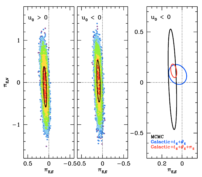
Figure 4: $\Delta\chi^{2}$ surfaces in $(\pi_{{\rm E},N},\pi_{{\rm E},E})$ plane. The left and middle distributions are drawn from the two solutions ($u_{0}>0$ and $u_{0}<0$). Except that $n=1$, the color coding is identical to that of Figure 2. In each panel, the black curve is the error contour $(\Delta\chi^{2}=1)$ extracted from the MCMC fit. The right panel shows the evolution of the parallax vector ($u_{0}<0$) depending on the priors. The blue curve is the posterior distribution $(-2\Delta\ln{\cal L}=1)$ derived from the timescale and angular Einstein radius constraints, while the red curve is based on the additional parallax constraint (see Section 4).

The results are presented in Table 1. We find that the fit improvement from these higher-order effects is $\Delta\chi^{2}\sim 9$, which has a Gaussian false probability (from four extra degrees of freedom) of just $(1+\Delta\chi^{2}/2)\exp(-\Delta\chi^{2}/2)=6\%$. This low level of improvement implies that it is difficult to directly determine the characteristics of the lens system from the microlensing fit parameters alone. Hence, we constrain the physical lens properties from a Bayesian analysis based on Galactic models. At this point, one might suggest that it is needless to introduce the measured higher-order effects to the analysis, but rather the lens system should be estimated only from the standard solution. However, this point of view is not always correct. As discussed in Han et al. (2016), we know a priori that all binary microlenses have both finite microlens parallax and finite lens orbital motion. This indicates that even in such low- or non-measurement cases, well-constrained higher-order parameters can include considerable information about the lens system. Hence, they can play an important role in constraining the physical lens properties from statistical analyses. In our case, we find that the east component of parallax vector $\pi_{{\rm E},E}$ is well constrained for both the $u_{0}>0$ and $u_{0}<0$ solutions, although the error of the north component $\pi_{{\rm E},N}$ is considerable (see Figure 4). In addition, we find that for both parallax solutions (as well as the standard, no-parallax solution), the seven standard parameters (except the sign of $u_{0}$) are consistent within $1\sigma$, which implies that the existence of multiple solutions does not significantly affect the statistical expectation of the lens system. Therefore, in what follows, we show results of the Bayesian analysis only for $u_{0}<0$ solution. However, we note that the results for the $u_{0}>0$ solution are nearly identical.

4 Physical Parameters

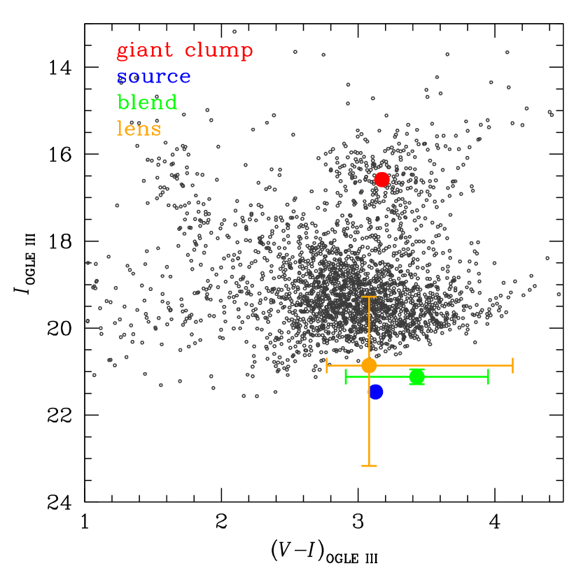
Figure 5: Calibrated color-magnitude diagram of field stars around KMT-2017-BLG-0165. The locations of microlensed source and giant clump centroid (GC) are marked by the blue and red points, respectively. The orange point shows the color and magnitude expected on the basis of the mass and distance derived from the Bayesian analysis. The green point indicates the position of the blended light estimated from the CFHT $r$- and $i$-band images. The astrometric position of the blend is well aligned with the source. See Figure 7. Hence it is plausible that the blended light is due to the lens. See text.

Our first step for constraining the physical lens parameters is to determine the angular Einstein radius $\theta_{\rm E}$. For this, we adopt the method of Yoo et al. (2004). We derive the source color $(V-I)_{\rm S}$ and brightness $I_{\rm S}$ from the model using the KMTNet star catalog calibrated to the OGLE-III photometry map (Szymański et al., 2011). We then measure the source offset from the giant clump centroid (GC) in the color-magnitude diagram (CMD): $\Delta(V-I,~{}I)=(V-I,~{}I)_{\rm S}-(V-I,~{}I)_{\rm GC}=(2.53\pm 0.04,~{}18.43\pm 0.02)-(2.58\pm 0.03,~{}13.54\pm 0.02)=(-0.05\pm 0.05,~{}4.89\pm 0.03)$. Figure 5 shows the positions of source and GC in the CMD. We find the dereddened source position as

$$(V-I,~{}I)_{0,{\rm S}}=\Delta(V-I,~{}I)+(V-I,~{}I)_{0,{\rm GC}}=(1.01\pm 0.09,~{}19.25\pm 0.09),$$ (6)

where $(V-I,~{}I)_{0,{\rm GC}}=(1.06\pm 0.07,14.37\pm 0.09)$ is the dereddened GC position adopted from Bensby et al. (2013) and Nataf et al. (2013), respectively. We convert our estimated $(V-I)_{0,{\rm S}}$ to $(V-K)_{0,{\rm S}}=2.30\pm 0.09$ using the $VIK$ relation (Bessell & Brett, 1988), and then derive the angular source radius

$$\theta_{*}=0.63\pm 0.06~{}\mu{\rm as}$$ (7)

using the $(V-K)-\theta_{*}$ relation (Kervella et al., 2004). Here, the error in $\theta_{*}$ is estimated from the uncertainty of the source color measurement (4%), centroiding the giant clump (7%), and the color-surface brightness conversion (5%). From the measured source radius $\rho_{*}$, we finally derive the angular Einstein radius

$$\theta_{\rm E}={\theta_{*}\over\rho_{*}}=0.80\pm 0.13~{}{\rm mas},$$ (8)

which corresponds to the geocentric lens-source relative proper motion

$$\mu_{\rm geo}={\theta_{\rm E}\over t_{\rm E}}=6.93\pm 1.15~{}{\rm mas~{}yr^{-1}}.$$ (9)

With the measured $t_{\rm E}$, $\theta_{\rm E}$, and $\pi_{\rm E}$ constraints, we conduct a Bayesian analysis by adopting the procedure and Galactic model of Jung et al. (2018). We first create a large sample of lensing events that are randomly drawn from the Galactic model. For each trial event, we then evaluate the likelihood of the microlensing parameters $(t_{\rm E},\theta_{\rm E},\pi_{{\rm E},N},\pi_{{\rm E},E})_{k}$ that are explicitly predicted by each combination of simulated lens and source properties. If all four of these parameters were uncorrelated, the likelihood of the event given the model could be estimated by a product of four Gaussian distributions. However, while the correlations between $(t_{\rm E},\theta_{\rm E})$, $(t_{\rm E},\mbox{\boldmath$\pi$}_{\rm E})$, and $(\theta_{\rm E},\mbox{\boldmath$\pi$}_{\rm E})$ are all quite weak, the correlation between $(\pi_{{\rm E},N},\pi_{{\rm E},E})$ can be quite strong (Gould, 2004). Therefore, we estimate the likelihood as the product of a bivariate Gaussian of $(\pi_{{\rm E},N},\pi_{{\rm E},E})$ with two univariate Gaussians of $t_{\rm E}$ and $\theta_{\rm E}$. For this, we evaluate the $\chi^{2}$ difference between the simulated and the measured values as

$$\chi_{{\rm gal},k}^{2}=\chi_{k}^{2}(t_{\rm E})+\chi_{k}^{2}(\theta_{\rm E})+\chi_{p,k}^{2};~{}~{}~{}~{}~{}\chi_{p,k}^{2}=\sum(a_{k}-a_{0})_{i}c_{ij}^{-1}(a_{k}-a_{0})_{j},$$ (10)

where $\mathbf{a}_{k}=\mbox{\boldmath$\pi$}_{{\rm E},k}=(\pi_{{\rm E},N},~{}\pi_{{\rm E},E})_{k}$, and $a_{0}$ and $c$ are the mean value of $\mbox{\boldmath$\pi$}_{\rm E}$ and its covariance matrix extracted from the MCMC, respectively. We then estimate the relative likelihood of the event by

$${\rm P}_{k}={\rm exp}(-\chi_{{\rm gal},k}^{2}/2)\times\Gamma_{k},$$ (11)

where $\Gamma_{k}\propto\theta_{{\rm E},k}\mu_{k}$ is the microlensing event rate. Finally, we explore the likelihood distributions of the lens properties from all trial events using ${\rm P}_{k}$ as a prior. We note that to show the contributions of individual constraints for estimating the physical lens properties, we additionally explore the distributions (1) with only the $t_{\rm E}$ constraint and (2) with the $t_{\rm E}$ and $\theta_{\rm E}$ constraints.

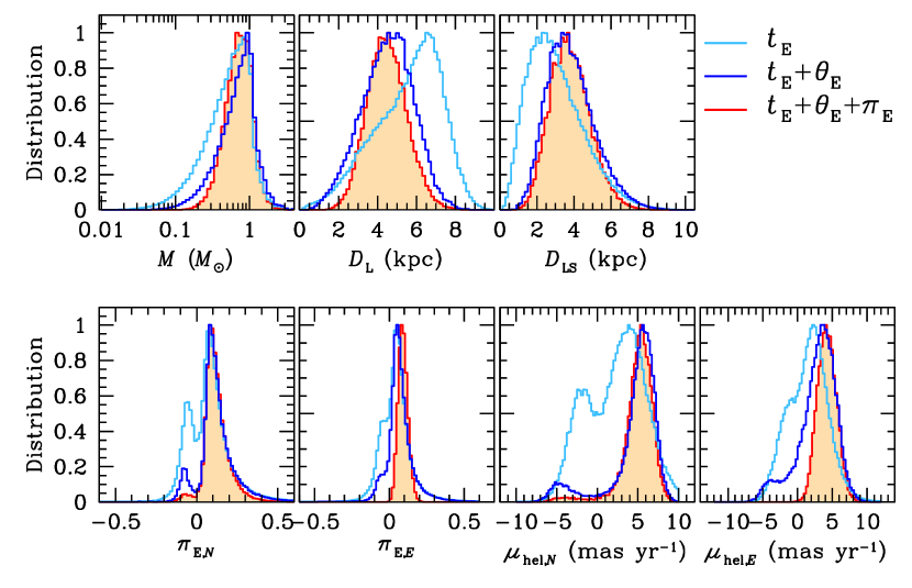
Figure 6: Likelihood distributions of the lens properties derived from the Bayesian analysis. In each panel, the three curves with light blue, blue, and red colors show the distributions derived from the timescale constraint, the timescale and angular Einstein constraints, and the additional parallax constraint, respectively. The distributions are for the $u_{0}<0$ solution, but those for the $u_{0}>0$ and no-parallax solutions are virtually identical.

The results are shown in Figure 6. We find that the measured $\pi_{\rm E}$ and $\theta_{\rm E}$ provide a strong constraint on the distributions (see the right panel in Figure 4). The median values of the lens host-mass $M_{1}$ and distance $D_{\rm L}$ with $68\%$ confidence intervals are

$$M_{1}={0.76}_{-0.27}^{+0.34}~{}M_{\odot},~{}~{}~{}~{}~{}D_{\rm L}={4.53}_{-0.98}^{+1.04}~{}{\rm kpc},$$ (12)

respectively. The corresponding heliocentric source proper motion relative to the lens are

$$\mu_{\rm hel}=\left|\mbox{\boldmath$\mu$}_{\rm geo}+{\mathbf{v}}_{\oplus,\perp}{\pi_{\rm rel}\over{\rm AU}}\right|=6.93_{-1.54}^{+1.38}~{}{\rm mas\,yr^{-1}},$$ (13)

where ${\mathbf{v}}_{\oplus,\perp}=(v_{\oplus,N},v_{\oplus,E})=(2.21,10.42)~{}{\rm km\,s^{-1}}$ is Earth’s projected velocity at $t_{0}$. Combined with the lens-source distance $D_{\rm LS}=3.80_{-1.00}^{+1.13}~{}{\rm kpc}$, these indicate that the lens host is a Sun-like star located in the Galactic disk. The mass of the planet and its projected separation from the host are then estimated by

$$M_{2}=qM_{1}=34_{-12}^{+15}~{}M_{\oplus},~{}~{}~{}~{}~{}a_{\bot}=s{D_{\rm L}}{\theta_{\rm E}}=3.45_{-0.95}^{+0.98}~{}{\rm AU}.$$ (14)

That is, the planet is a cold super-Neptune lying outside the snowline of the host, i.e., $a_{sl}=2.7\,{\rm AU}(M/M_{\odot})\sim 2.1\,{\rm AU}$. We summarize the estimated lens properties including the measured $\theta_{\rm E}$, $\mu_{\rm geo}$, and $\mbox{\boldmath$\mu$}_{\rm hel}$ in Table 2.

We now investigate whether these Bayesian estimates of the lens physical properties imply a lens flux that is consistent with the blended light at the position of the microlensed source. This comparison requires two distinct steps. First, we must place the lens-flux estimates on the calibrated CMD (Figure 5). Second, we must make a refined estimate of the blended light and place this estimate on the same calibrated CMD. Based on the lens host-mass, we first estimate the absolute brightness of the lens in $I$ band as $M_{I}=5.37_{-1.58}^{+2.31}$ (Pecaut & Mamajek, 2013). Because the lens distance is $D_{\rm L}\sim 4.5~{}{\rm kpc}$, it is expected that the lens is probably behind most of the dust in the disk. Hence, we assume that the lens experiences similar reddening and extinction to those of the microlensed source. The lens position in the CMD is then estimated by

$$(V-I,I)_{\rm L}=(V-I,I)_{0,\rm L}+(V-I,I)_{\rm GC}-(V-I,I)_{0,{\rm GC}}=(3.08_{-0.31}^{+1.05},20.86_{-1.58}^{+2.31}),$$ (15)

where $I_{0,{\rm L}}=M_{I}+5{\rm log}(D_{\rm L}/{\rm pc})-5$ and $(V-I)_{0,\rm L}=0.97_{-0.31}^{+1.05}$ is the intrinsic color of the lens adopted from Pecaut & Mamajek (2013).

The blended light cannot be accurately estimated either from the KMTNet reference image or from the source characteristics listed in the OGLE-III catalog (Szymański et al., 2011) that is used to identify microlensed sources by the KMTNet event-finder (Kim et al., 2018), because the source star is not resolved in either image. That is, the OGLE-III-based catalog star lies $0.6^{\prime\prime}$ from the microlensed source and thus this catalog star must be a blend of the source, the lens, as well as one or more stars that are substantially displaced from these objects. Similarly, there is no distinct “star” at the location of the event in the KMTNet reference image. However, we find that high-resolution images of KMT-2017-BLG-0165 were observed by the 2016 CFHT-K2C9 Multi-color Microlensing Survey (Zang et al., 2018), a special survey designed to measure the colors of microlensed sources for K2’s Campaign 9 microlensing survey (Henderson et al., 2016) with the $g$-, $r$-, and $i$-band filters of the Canada-France-Hawaii Telescope (CFHT) on Mauna Kea. Therefore, we make use of these $0.187^{\prime\prime}$ pixel images, which have FWHM $\sim 0.5^{\prime\prime}$.

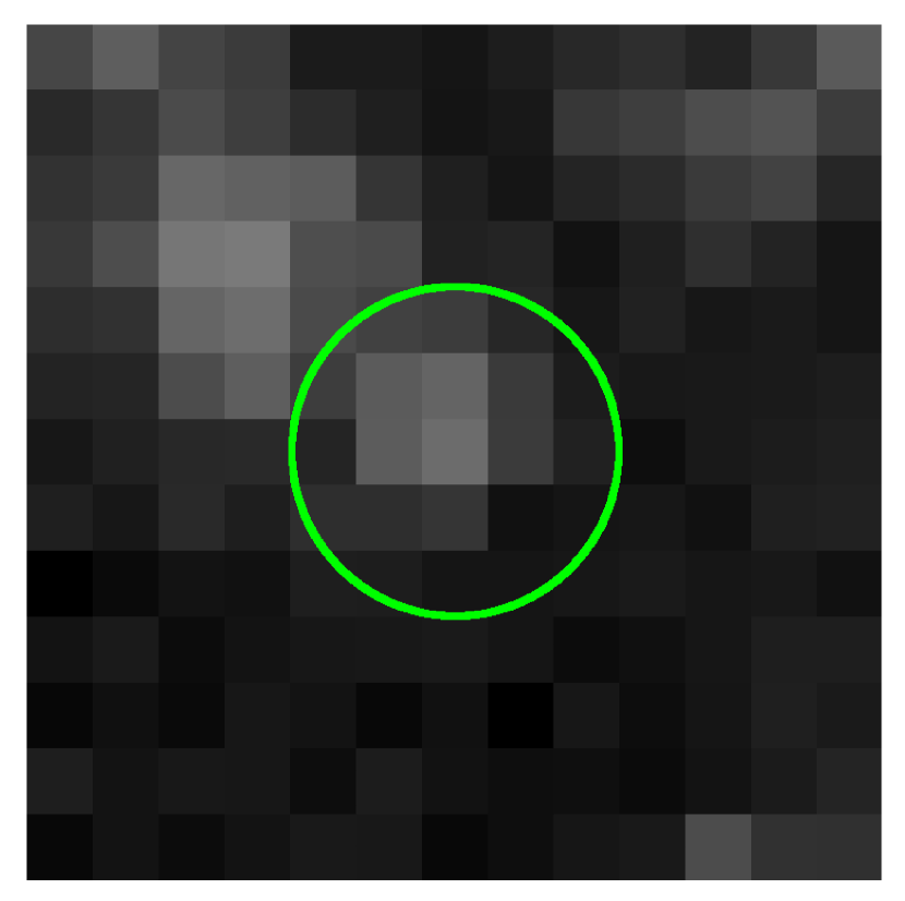
Figure 7: $i$-band CFHT image within $2.4^{\prime\prime}\times 2.4^{\prime\prime}$ around the event. The green circle indicates the source position derived from the astrometric transformation of a highly magnified KMTNet image.

To estimate the blended light, we first identify the source position in the CFHT images from an astrometric transformation of a highly magnified KMTNet image. Figure 7 shows one of these images together with the position of the source circled in green. We find that the “baseline object” associated with the source and lens (and possibly other stars) is clearly resolved in the $r$- and $i$-band images. We then perform aperture photometry and align it to the calibrated OGLE-III system shown in Figure 5. From this, we find $V_{\rm base}=23.82\pm 0.24$ and $I_{\rm base}=20.53\pm 0.09$. Subtracting the source flux (from the model fit) yields the $(V-I)$ color and $I$-band magnitude of the blended light as $(V-I,I)_{\rm b}=(3.43\pm 0.52,21.12\pm 0.17)$. We then plot this value in green on the CMD (see Figure 5). We see from Figure 5 that the blended flux (green) is quite consistent (within $1\sigma$) with the flux predicted for the lens (orange). The relation of the blended light to the lens could be further investigated using adaptive optics (AO) follow up.

5 Discussion

KMT-2017-BLG-0165Lb is a planet with a mass-ratio of $q=1.3\times 10^{-4}$, which is near the Suzuki et al. (2016) break, $q_{\rm br}=1.7\times 10^{-4}$. In this context, we investigate the location ($q_{\rm br}$) and strength ($\zeta$) of the mass-ratio break from the distribution of microlensing planets in the region of the break: $q\leq 3.0\times 10^{-4}$. For this, we first review the literature and find the planets whose mass ratios are securely measured (without any strong degeneracy) and lie below $q=3.0\times 10^{-4}$. We find 15 planets (including KMT-2017-BLG-0165Lb) that satisfy these criteria. Table 3 gives the main characteristics of these planets. We note that there is another planetary event, OGLE-2017-BLG-0173 (Hwang et al., 2018), whose mass ratio falls in the defined range. However, the event suffers from large uncertainties in the mass ratio measurement due to a discrete degeneracy between two classes of solutions, i.e., $q=(2.5,6.5)\times 10^{-5}$. Whenever two solutions with different mass ratios are roughly equally consistent with the data, including such planets in the analysis would mean that their role depends on the priors. In our case, however, we do not have independent (prior) knowledge of the mass-ratio function, and this is what we are trying to measure. Therefore, we exclude the event in order to obtain reliable independent results.

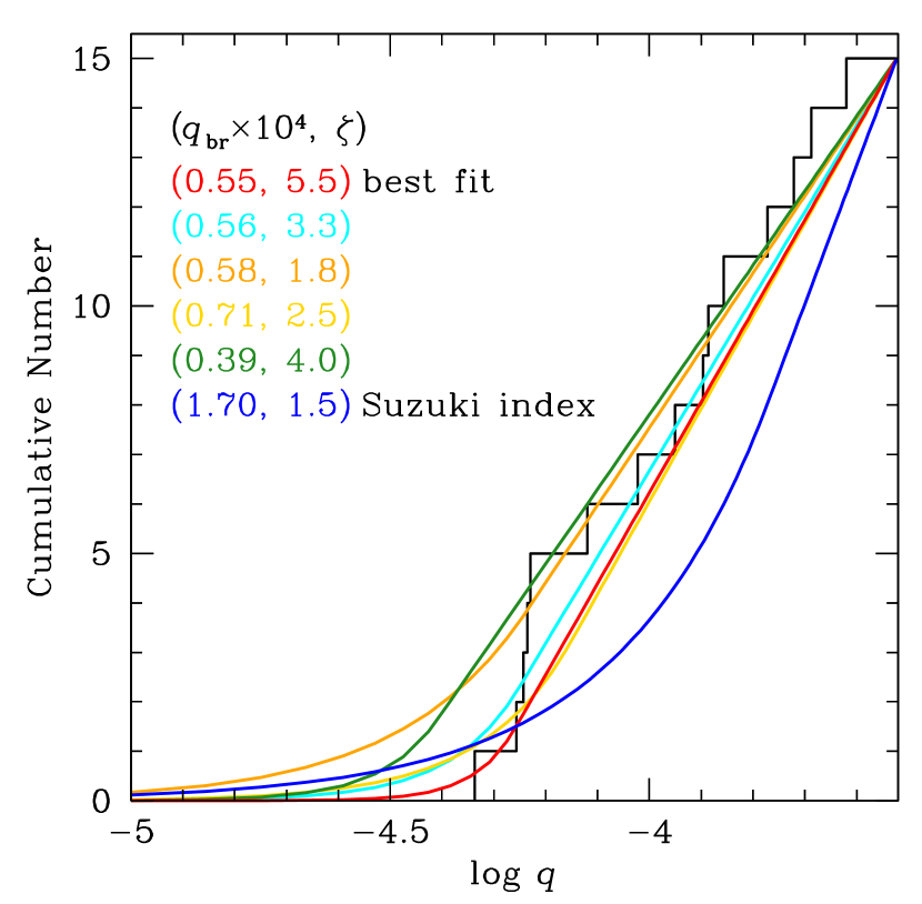
Figure 8: Cumulative distribution of the mass ratio $q$ in the regime of $q<3\times 10^{-4}$. The black curve is the actual cumulative distribution of fifteen microlensing planets. The blue curve is the predicted distribution based on the result of Suzuki et al. (2016), while the remaining curves are some representative (including the best fit) distributions derived from the likelihood ${\cal L}$ analysis.

We find that the cumulative distribution in our sample domain $(4\times 10^{-5}<q<3\times 10^{-4})$ is primarily characterized by a straight line, which corresponds to a uniform distribution in ${\rm log}~{}q$ over $\Delta\log q=0.875$ decades, i.e., $dN_{\rm obs}/d\log q={\rm const}$ (see Figure 8). The most notable feature within this overall trend is a “pile up” of four planets in the short interval ($\Delta\log q=0.030$ decades) at $5.5\times 10^{-5}<q<5.9\times 10^{-5}~{}(-4.26<{\rm log}~{}q<-4.23)$.

Next, we calculate the cumulative distribution for a broken power law. We begin by considering that the intrinsic occurrence rate of planets across the whole range that is being probed follows a power-law function $f_{0}({\rm log}~{}q)=dN_{0}/d{\rm log}~{}q\sim q^{\alpha}$. We must also consider the sensitivity of microlensing experiments to planets, which we assume is a power law. The observed planet frequency is then

$$f_{\rm obs}({\rm log}~{}q)={dN_{\rm obs}\over d{\rm log}~{}{q}}=f_{0}({\rm log}~{}q)S(q)\sim q^{\alpha+\beta}.$$ (16)

For our calculation, we adopt that the cumulative distribution is linear, i.e., constant number of detections in each bin of equal ${\rm log}~{}q$ (Mróz et al., 2017a). This means that the frequency is flat, i.e., $f_{\rm obs}({\rm log}~{}q)\sim q^{0}$. That is, $\alpha=-\beta$. We then apply the broken power-law function as a form of

$$g_{0}({\rm log}~{}q)=K\left({q\over q_{\rm br}}\right)^{\alpha}~{}(q>q_{\rm br});~{}~{}~{}~{}~{}g_{0}({\rm log}~{}q)=K\left({q\over q_{\rm br}}\right)^{\alpha+\zeta}~{}(q<q_{\rm br}),$$ (17)

where $K$ is a normalization constant. The observed planet frequency for the broken power-law $g_{\rm obs}({\rm log}~{}q)=g_{0}({\rm log}~{}q)S(q)$ is then given by

$$g_{\rm obs}({\rm log}~{}q)=K~{}(q>q_{\rm br});~{}~{}~{}~{}~{}g_{\rm obs}({\rm log}~{}q)=K\left({q\over q_{\rm br}}\right)^{\zeta}~{}(q<q_{\rm br}).$$ (18)

Finally, we derive the cumulative distribution function $G_{\rm obs}({\rm log}~{}q)=\int_{0}^{q}g_{\rm obs}({\rm log}~{}q^{\prime})d{\rm log}~{}q^{\prime}$ as

$$G_{\rm obs}({\rm log}~{}q)=K\left[{1\over\zeta}+{\rm ln}\left({q\over q_{\rm br}}\right)\right]~{}(q>q_{\rm br});~{}~{}~{}~{}~{}G_{\rm obs}({\rm log}~{}q)={K\over\zeta}\left({q\over q_{\rm br}}\right)^{\zeta}~{}(q<q_{\rm br}).$$ (19)

Here, we find the constant $K$ by matching this function to the actual cumulative distribution, i.e.,

$$K={G_{\rm max}\over 1/\zeta+{\rm ln}(q_{\rm max}/q_{\rm br})},$$ (20)

where $G_{\rm max}=G_{\rm obs}({\rm log}~{}q_{\rm max})=G_{\rm obs}[{\rm log}~{}(3\times 10^{-4})]=15$. Therefore, for a given mass ratio $q$, the predicted cumulative distribution $G_{\rm obs}({\rm log}~{}q)$ can be determined as a function of $\zeta$ and $q_{\rm br}$.

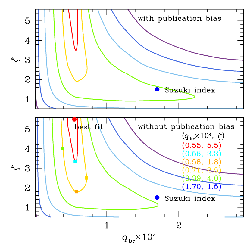
Figure 9: $-2\Delta\ln{\cal L}$ contour in $(q_{\rm br},~{}\zeta)$ plane. The lower and upper panels show the distributions derived without and with the “publication bias” adjustment, respectively. The red point is the location of best-fit model, while the blue point is the location of Suzuki et al. (2016) index. The squares with different colors are the positions of some representative models shown in Figure 8. The color coding is identical to that of Figure 2, except that $n=1$.

Next, we calculate the likelihood ${\cal L}$ of the observed 15 planets given model functions defined by two parameters $(q_{\rm br},\zeta)$. In Figure 9, we show the contours of the result according to $-2\Delta\ln{\cal L}=(1,4,9,16,25,36)$. The cumulative distributions for some representative models are also shown in Figure 8. The best fit $(q_{\rm br}\times 10^{4},\zeta)=(0.55,5.5)$ is shown as a red curve. Because $q_{\rm br}=0.55\times 10^{-4}$ is below all but two of the observed planets, this model matches the observed (flat) distribution quite well. We find that the model accounts for the absence of observed planets $q<4.6\times 10^{-4}$ by an extremely strong power-law break, $\zeta=5.5$. As shown in Figure 9, we also find that the probable (i.e., “$1\,\sigma$”) models all have this same break point $q_{\rm br}\simeq 0.55\times 10^{-4}$. The lowest strength for probable models is $\zeta=3.3$ (see the cyan curve in Figure 8). That is, all of these models require an extremely sharp power-law break, which corresponds approximately to a cut off just below $q_{\rm br}$.

We note that from our sample planets, we identify a bias, so-called “publication date” bias (Mróz et al., 2017a). We find that on average, the three planets with $q>1.7\times 10^{-4}$ show a five year delay for their publications relative to their discovery years, while the planets at lower $q$ show only a one-year delay. In order to check whether our result can be affected by this bias, we additionally calculate the likelihood distribution with the “publication bias” adjustment, for which we weight the counts of those three planets by a factor of 1.5 , i.e., $G_{\rm max}=16.5$. From this, we find that the derived distribution is virtually identical to that derived without the adjustment (see Figure 9).

Our result is quite different from that of Suzuki et al. (2016). First, the break is at much lower mass ratio than their best value: $q_{\rm br}=1.7\times 10^{-4}$. Second, the break is also much stronger than their adopted range $\zeta=1.5^{+0.5}_{-0.4}$. We find that both of these characteristics follow directly from the observed cumulative distribution shown in Figure 8. As noted above, the straight-line cumulative distribution corresponds to detections that are uniform in $\log q$, and these detections simply stop below the $x$-intercept of this straight line. This implies more of a “cut off” than a break in the power-law index. Within the context of broken-power-law models, this “cut off” is then mathematically manifested as a very steep break in the index just above the lowest-$q$ detection.

The slope we find is also different from the estimate by Udalski et al. (2018), who derived a value similar to that of Suzuki et al. (2016). This difference is due to the difference in the configuration used for the analysis. Instead of looking for the position of the break, Udalski et al. (2018) assumed that the break is placed above $q>10^{-4}$ and that the mass-ratio function below $q<10^{-4}$ has the form of a power law. With these assumptions, they only investigated the index of this power law using the seven planets in the $q<10^{-4}$ regime. By contrast, we seek to not only identify the position of the break in the power law but also find the change of the power-law slope between mass ratios above and below the break. As presented above, our estimated break is at $q_{\rm br}=0.55\times 10^{-4}$, corresponding to the middle of the Udalski et al. (2018) sample. This contradicts their assumption that the break occurs above $q>10^{-4}$. Therefore, it is inevitable that the conclusions are different.

In principle, the complete absence of detections for $q<0.4\times 10^{-4}$ could be due to a catastrophic decline in microlensing sensitivity to such low-mass-ratio planets. However, Udalski et al. (2018) studied the sensitivity of the seven events with $q<10^{-4}$, and found that microlensing studies can probe planets in the regime quite well, where (as shown in Figure 8) there are no actual detected planets. Hence, this suggests that the absence of detected planets in this mass-ratio regime reflects their paucity in nature.

We next ask: is the “pile up”of four planets within $\Delta\log q=0.03$, mentioned above, real? It is difficult to devise reliable statistical tests for such posteriori “features”. A simple Kolmogorov-Smirnov (KS) test ($D=0.2$ for an $n=15$ sample) yields a false probability of $p=12\%$. This is certainly not strong enough to reject the class of broken-power-law models. On the other hand, there is no a priori reason that the planet mass-ratio frequency should follow a broken power law. In particular, physically based models could plausibly account for a pile-up at Neptune-like mass ratios because this is near to the point that a rock/ice core can start to accumulate a gaseous envelop. Therefore, we suggest that the apparent “pile up” in Figure 8 may be real and warrants further investigation as more statistics are accumulated.

Table 1: Lensing Parameters

Parameters	Standard	Orbit+Parallax
		$u_{0}>0$	$u_{0}<0$
$\chi^{2}$/dof	30210.9/30182	30202.1/30178	30201.6/30178
$t_{0}$ (${\rm HJD^{\prime}}$)	7853.73$\pm$ 0.063	7853.72$\pm$ 0.065	7853.71 $\pm$ 0.067
$u_{0}$	0.034 $\pm$ 0.010	0.036 $\pm$ 0.011	-0.035 $\pm$ 0.011
$t_{\rm E}$ (days)	43.105 $\pm$ 0.771	41.775 $\pm$ 0.846	42.129 $\pm$ 0.932
$s$	0.951 $\pm$ 0.009	0.953 $\pm$ 0.012	0.953 $\pm$ 0.013
$q$ ($10^{-4}$)	1.392 $\pm$ 0.036	1.332 $\pm$ 0.086	1.348 $\pm$ 0.090
$\alpha$ (rad)	5.821 $\pm$ 0.029	5.817 $\pm$ 0.032	-5.821 $\pm$ 0.033
$\rho_{\ast}$ ($10^{-4}$)	7.863 $\pm$ 0.759	7.709 $\pm$ 1.029	7.834 $\pm$ 1.072
$\pi_{{\rm E},N}$	–	0.049 $\pm$ 0.457	-0.099 $\pm$ 0.471
$\pi_{{\rm E},E}$	–	0.088 $\pm$ 0.041	0.108 $\pm$ 0.040
$ds/dt$ (yr-1)	–	0.416 $\pm$ 1.183	-0.745 $\pm$ 1.204
$d\alpha/dt$ (yr-1)	–	0.369 $\pm$ 0.272	0.531 $\pm$ 0.276
$f_{\rm s}$	0.038 $\pm$ 0.003	0.040 $\pm$ 0.003	0.040 $\pm$ 0.003
$f_{\rm b}$	0.125 $\pm$ 0.009	0.124 $\pm$ 0.009	0.124 $\pm$ 0.009

Note. — ${\rm HJD}^{\prime}={\rm HJD}-2450000$

Table 2: Lens properties

Parameters	Values
$\theta_{\rm E}$ (mas)	0.80$\pm$0.13
$\mu_{\rm geo}$ $({\rm mas}\,{\rm yr}^{-1})$	6.93$\pm$1.15
$\mu_{\rm hel}$ $({\rm mas}\,{\rm yr}^{-1})$	$6.93_{-1.54}^{+1.38}$
$\mu_{{\rm hel},N}$ $({\rm mas}\,{\rm yr}^{-1})$	$5.41_{-1.65}^{+1.35}$
$\mu_{{\rm hel},E}$ $({\rm mas}\,{\rm yr}^{-1})$	$4.33_{-1.36}^{+1.42}$
$M_{1}$ $(M_{\odot})$	$0.76_{-0.27}^{+0.34}$
$M_{2}$ $(M_{\oplus})$	$34_{-12}^{+15}$
$D_{\rm L}$ (kpc)	$4.53_{-0.98}^{+1.04}$
$a_{\bot}$ (AU)	$3.45_{-0.95}^{+0.98}$

Table 3: Characterisitcs of planets

Event	$q(10^{-4})$	$s$	$M_{\rm p}/M_{\oplus}$	$M_{\rm h}/M_{\odot}$	$D_{\rm L}/{\rm kpc}$	$a_{\perp}/{\rm AU}$	Discovery paper
OGLE-2013-BLG-0341	0.46	0.81	2.00	0.15	1.16	0.88	Gould et al. (2014)
OGLE-2016-BLG-1195	0.55	0.98	1.43	0.08	3.91	1.16	Shvartzvald et al. (2017)
OGLE-2017-BLG-1434	0.57	0.98	4.48	0.23	0.87	1.18	Udalski et al. (2018)
MOA-2009-BLG-266	0.58	0.91	10.40	0.56	3.04	3.20	Muraki et al. (2011)
OGLE-2005-BLG-169	0.59	1.02	14.10	0.69	4.10	3.50	Gould et al. (2006)†
OGLE-2005-BLG-390	0.76	1.61	5.50	0.22	6.60	2.60	Beaulieu et al. (2006)
OGLE-2007-BLG-368	0.95	0.93	20.00	0.64	5.90	2.80	Sumi et al. (2010)
MOA-2007-BLG-192	1.20	1.12	3.30	0.06	1.00	0.62	Bennett et al. (2008)
MOA-2011-BLG-028	1.27	1.69	30.00	0.75	7.38	4.14	Skowron et al. (2016)
OGLE-2012-BLG-0026	1.30	1.03	46.07	1.06	4.02	4.00	Han et al. (2013)
KMT-2017-BLG-0165	1.35	0.95	34.00	0.76	4.53	3.45	this work
OGLE-2015-BLG-0966	1.69	1.12	21.00	0.38	2.50	2.10	Street et al. (2016)
OGLE-2012-BLG-0950	1.90	1.00	35.00	0.56	3.00	2.70	Koshimoto et al. (2017)
MOA-2012-BLG-505	2.05	1.13	6.70	0.10	7.21	0.91	Nagakane et al. (2017)
OGLE-2008-BLG-092	2.41	5.26	43.60	0.71	8.10	18.00	Poleski et al. (2014)

Note. — ^† For OGLE-2005-BLG-169, the values are obtained from Bennett et al. (2015), who refined the solution from follow-up observations of the lens and the source stars using the Hubble Space Telescope (HST) Wide Field Camera 3 (WFC3).

References

- Alard & Lupton (1998) Alard, C., & Lupton, Robert H. 1998, ApJ, 503, 325
- Albrow et al. (2009) Albrow, M. D., Horne, K., Bramich, D. M., et al. 2009, MNRAS, 397, 2099
- Batista et al. (2011) Batista, V., Gould, A., Dieters, S., et al. 2011, A&A, 529, 102
- Beaulieu et al. (2006) Beaulieu, J.-P., Bennett, D. P., & Fouqué, P. 2006, Nature, 439, 437
- Bennett et al. (2015) Bennett, D. P., Bhattacharya, A., Anderson, J., et al. 2015, ApJ, 808, 169
- Bennett et al. (2008) Bennett, D. P., Bond, I. A., Udalski, A., et al. 2008, ApJ, 684, 663
- Bensby et al. (2013) Bensby, T., Yee, J. C., Feltzing, S., et al. 2013, A&A, 549, 147
- Bessell & Brett (1988) Bessell, M. S., & Brett, J. M. 1988, PASP, 100, 1134
- Cassan et al. (2012) Cassan, A., Kubas, D., Beaulieu, J.-P., et al. 2012, Nature, 481, 167
- Dominik (1998) Dominik, M. 1998, A&A, 329, 361
- Dong et al. (2009) Dong, S., Gould, A., Udalski, A., et al. 2009, ApJ, 695, 970
- Gaudi (2012) Gaudi, B. S. 2012, ARA&A, 50, 411
- Gould (1992) Gould, A. 1992, ApJ, 392, 442
- Gould (2004) Gould, A. 2004, ApJ, 606, 319
- Gould (2008) Gould, A. 2008, ApJ, 681, 1593
- Gould & Loeb (1992) Gould, A., & Loeb, A. 1992 ApJ, 306, 104
- Gould et al. (2010) Gould, A., Dong, S., Gaudi, B. S., et al. 2010, ApJ, 720, 1073
- Gould et al. (2006) Gould, A., Udalski, A., An, D. 2006, ApJ, 644, L37
- Gould et al. (2014) Gould, A., Udalski, A., Shin, I.-G., et al. 2014, Sci, 345, 46
- Han (2006) Han, C. 2006, ApJ, 638, 1080
- Han et al. (2013) Han, C., Udalski, A., Choi, J.-Y., et al. 2013, ApJ, 762, L28
- Han et al. (2016) Han, C., Udalski, A., Gould, A., et al. 2016, ApJ, 828, 53
- Henderson et al. (2016) Henderson, C. B., Poleski, R., Penny, M., et al. 2016, PASP, 128, 124401
- Hwang et al. (2018) Hwang, K.-H., Udalski, A., Shvartzvald, Y., et al. 2018, AJ, 155, 20
- Ida & Lin (2004) Ida, S., & Lin, D. N. C. 2004, ApJ, 616, 567
- Jung et al. (2013) Jung, Y. K., Han, C., Gould, A., & Maoz, D. 2013, ApJ, 768, L7J
- Jung et al. (2018) Jung, Y. K., Udalski, A., Gould, A., et al. 2018, AJ, 155, 219
- Jung et al. (2015) Jung, Y. K., Udalski, A., Sumi, T., et al. 2015, ApJ, 798, 123
- Kayser et al. (1986) Kayser, R., Refsdal S., & Stabell, R. 1986, A&A, 166, 36
- Kervella et al. (2004) Kervella P., Thévenin F., Di Folco E., Ségransan D., 2004, A&A, 426, 297
- Kim et al. (2016) Kim, S.-L., Lee, C.-U., Park, B.-G., et al. 2016, JKAS, 49, 37
- Kim et al. (2018) Kim, D.-J., Kim, H.-W., Hwang, K.-H., et al. 2018, AJ, 155, 76
- Koshimoto et al. (2017) Koshimoto, N., Udalski, A., Beaulieu, J. P., et al. 2017, AJ, 153, 1
- Mróz et al. (2017a) Mróz, P., Han, C., Udalski, A., et al. 2017a, AJ, 153, 143
- Mróz et al. (2018) Mróz, P., Ryu, Y.-H., Skowron, J., et al. 2018, AJ, 155, 121
- Mróz et al. (2017b) Mróz, P., Udalski, A., Skowron, J. et al. 2017b, Nature, 548, 183
- Muraki et al. (2011) Muraki, Y., Han, C., Bennett, D. P., et al. 2011, ApJ, 741, 22
- Nagakane et al. (2017) Nagakane, M., Sumi, T., Koshimoto, N., et al. 2017, AJ, 154, 35
- Nataf et al. (2013) Nataf, D. M., Gould, A., Fouqué, P., et al. 2013, ApJ, 769, 88
- Paczyński (1986) Paczyński, B. 1986, ApJ, 304, 1
- Pecaut & Mamajek (2013) Pecaut, M. J., & Mamajek, E. E. 2013, ApJS, 208, 9
- Pejcha & Heyrovský (2009) Pejcha, O., & Heyrovský, D. 2009, ApJ, 690, 1772
- Pepe et al. (2011) Pepe, F., Lovis, C., & Ségransan, D. 2011, A&A, 534, A58
- Poleski et al. (2014) Poleski, R., Skowron, J., Udalski, A., et al. 2014, ApJ, 795, 42
- Schneider & Weiss (1987) Schneider, P., & Weiss, A. 1987, A&A, 171, 49
- Shvartzvald et al. (2017) Shvartzvald, Y., Yee, J. C., Calchi Novati, S., et al. 2017, ApJ, 840, L3
- Skowron et al. (2011) Skowron, J., Udalski, A., Gould, A., et al. 2011, ApJ, 738, 87
- Skowron et al. (2016) Skowron, J., Udalski, A., Poleski, R., et al. 2016, ApJ, 820, 4
- Street et al. (2016) Street, R. A., Udalski, A., Calchi Novati, S., et al. 2016, ApJ, 819, 93
- Sumi et al. (2010) Sumi, T., Bennett, D. P., Bond, I. A., et al. 2010, ApJ, 710, 1641
- Sumi et al. (2011) Sumi, T., Kamiya, K., Bennett, D. P., et al. 2011, Nature, 473, 349
- Suzuki et al. (2016) Suzuki, D., Bennett, D. P., Sumi, T., et al. 2016, ApJ, 833, 145
- Szymański et al. (2011) Szymański, M. K., Udalski, A., Soszyński, I., et al. 2011, AcA, 61, 83
- Tenenbaum et al. (2014) Tenenbaum, P., Jenkins, J. M., Seader, S., et al. 2014, ApJS, 211, 6
- Udalski et al. (2018) Udalski, A., Ryu, Y.-H., Sajadian, S., et al. 2018, AcA, 68, 1
- Yoo et al. (2004) Yoo, J., DePoy, D. L., Gal-Yam, A., et al. 2004, ApJ, 603, 139
- Zang et al. (2018) Zang, W., Penny, M. T., Zhu, W., et al. 2018, PASP, submitted, arXiv:1803.09184
- Zhu et al. (2017) Zhu, W., Udalski, A., Calchi Novati, S., et al. 2017, AJ, 154, 210