An Online Updating Approach for Testing the Proportional Hazards Assumption with Streams of Survival Data

Abstract

The Cox model, which remains as the first choice in analyzing time-to-event data even for large datasets, relies on the proportional hazards (PH) assumption. When survival data arrive sequentially in chunks, a fast and minimally storage intensive approach to test the PH assumption is desirable. We propose an online updating approach that updates the standard test statistic as each new block of data becomes available, and greatly lightens the computational burden. Under the null hypothesis of PH, the proposed statistic is shown to have the same asymptotic distribution as the standard version computed on the entire data stream with the data blocks pooled into one dataset. In simulation studies, the test and its variant based on most recent data blocks maintain their sizes when the PH assumption holds and have substantial power to detect different violations of the PH assumption. We also show in simulation that our approach can be used successfully with “big data” that exceed a single computer’s computational resources. The approach is illustrated with the survival analysis of patients with lymphoma cancer from the Surveillance, Epidemiology, and End Results Program. The proposed test promptly identified deviation from the PH assumption that was not captured by the test based on the entire data.

Keywords: Cox model; Diagnostics; Schoenfeld residuals.

1 Introduction

Recent advances in information technology have made available data that arrive in high velocity everyday. Online methods, such as the online updating estimation and inference presented in Schifano et al. (2016), are appealing as storage of historical data is not required which yields great savings in computing resources. Survival data, or time-to-event data, may also arrive sequentially, and the desire for online updated inferences in the survival setting is not uncommon. For example, flight information, such as delay time until take-off or cancellation, is available for more than 114,000 commercial flights scheduled daily around the world (Air Transport Action Group, 2018); real estate information, such as time on market until sold, is updated continuously for the over 6 million homes in the real-estate market (National Association of Realtors, 2018). As such events occur everyday at high frequency, observations also accumulate quickly.

The Cox model (Cox, 1972) is the most commonly used tool in analyzing survival data. A crucial step in fitting the popular Cox model is to check the proportional hazards (PH) assumption (e.g., Xue and Schifano, 2017). The standard approach, if new data becomes available along a stream, would be to pool all historical data together, fit a new Cox model, and use standard methods such as the test of Grambsch and Therneau (1994) to examine whether the PH assumption is appropriate. This, however, can pose a heavy computational burden and can be very time-consuming when the data size gets large. While efforts have been made in fitting Cox model using distributed computing and therefore reducing the computing time, such as in Wang et al. (2019), methods for checking the PH assumption in these settings have not been developed.

In this work, we propose a method to test the PH assumption in the online updating setting, which does not require storage or access to the historical data. Our approach is an application of the divide-and-conquer and online updating strategies (Lin and Xi, 2011; Schifano et al., 2016) to the streaming survival data setting. The data is assumed to arrive sequentially in blocks, an the test statistic is an appropriately aggregated version of the standard test statistic of Grambsch and Therneau (1994) computed from each block. blocks. The statistics can be adapted to be based on data in a moving window of certain size, which may be more useful in detecting local deviations from the null hypothesis. A byproduct of our method is a cumulatively updated estimating equation (CUEE) estimator for the regression coefficients if the PH assumption is not rejected.

When the null hypothesis of PH is true, our test statistic is shown to have the same asymptotic distribution as the standard (full data) statistic under certain regularity conditions. In simulation studies, under the null hypothesis, the proposed test holds its size and the CUEE estimator closely approximates the estimator based on the full data; when the null hypothesis is not true, the test has comparable or higher power than the standard statistic based on the full data. For a dataset that can be loaded into computer memory, our proposed statistic can be computed in significantly less time than the standard statistic. Our test can also successfully be used within a reasonable amount of time for big data that cannot (easily) be loaded into memory. The method is illustrated by analyzing the survival time of the lymphoma cancer patients in the Surveillance, Epidemiology, and End Results (SEER) Program. Interestingly, while the changes in parameters were not captured by using the standard (full data) test of Grambsch and Therneau (1994), they were promptly identified by our online updated version.

The rest of this article is organized as follows. In Section 2, we review the notation of the Cox model and the test statistic of Grambsch and Therneau (1994). In Section 3, we propose our online updating test statistics for the PH assumption. We present simulation results in Section 4, and illustrate the usage of the test with an application to the survival time of patients with lymphoma cancer from the SEER data in Section 5. A discussion concludes in Section 6. The proposed methods are all implemented in R based on functions from the survival package (Therneau, 2015), and the code can be found via GitHub (Xue, 2018).

2 Cox Proportional Hazards Model

2.1 Notation and Preliminaries

For completeness we review the Cox model and tests for the PH assumption. Let $T_{i}^{*}$ be the true event time and $C_{i}$ be the censoring time for subject $i$. Define $T_{i}=\min(T_{i}^{*},C_{i})$ and $\delta_{i}=I(T_{i}^{*}\leq C_{i})$. Suppose we observe independent copies of $(\delta_{i},T_{i},{\boldsymbol{X}}_{i})$, $i=1,\ldots,n$, where ${\boldsymbol{X}}_{i}$ is the $p$-dimensional vector of covariates of the $i$th subject. The Cox model specifies the hazard for individual $i$ as

$$\lambda_{i}(t)=\lambda_{0}(t)\exp\left({\boldsymbol{X}}_{i}^{\top}{\boldsymbol{\beta}}\right),$$ (1)

where $\lambda_{0}$ is an unspecified non-negative function of time called the baseline hazard, and ${\boldsymbol{\beta}}$ is a $p$-dimensional coefficient vector in a compact parameter space. Because the logarithm of the hazard ratio for two subjects with fixed covariate vectors ${\boldsymbol{X}}_{i}$ and ${\boldsymbol{X}}_{j}$, $({\boldsymbol{X}}_{i}-{\boldsymbol{X}}_{j})^{\top}{\boldsymbol{\beta}}$, is proportional to the difference in covariate values and is otherwise constant over time (${\boldsymbol{\beta}}$), the model is also known as the PH model. It has been later extended to incorporate time-dependent covariates. For the rest of the article, we use ${\boldsymbol{X}}_{i}(t)$ to indicate the possibility of covariates being time-dependent.

Cox (1972, 1975) formulated the partial likelihood approach to estimate ${\boldsymbol{\beta}}$. For untied failure time data, Fleming and Harrington (1991) expressed it under the counting process formulation to be

$$\mathrm{PL}({\boldsymbol{\beta}})=\prod_{i=1}^{n}\prod_{t\geq 0}\left[\frac{Y_{i}(t)\exp\left\{{\boldsymbol{X}}_{i}(t)^{\top}{\boldsymbol{\beta}}\right\}}{\sum_{j}Y_{j}(t)\exp\left\{{\boldsymbol{X}}_{j}(t)^{\top}{\boldsymbol{\beta}}\right\}}\right]^{\differential N_{i}(t)},$$ (2)

where $Y_{i}(t)=I(T_{i}\geq t)$ is the at-risk indicator of the $i$th subject, $N_{i}(t)$ is the number of events for subject $i$ at time $t$, and $\differential N_{i}(t)=I(T_{i}\in[t,t+\Delta),\,\delta_{i}=1)$, with $\Delta$ sufficiently small such that $\sum_{i=1}^{n}\differential N_{i}(t)\leq 1$ for any $t$. Taking the natural logarithm of (2) gives the log partial likelihood in the form of a summation:

$$pl({\boldsymbol{\beta}})=\sum_{i=1}^{n}\int_{0}^{\infty}\left[Y_{i}(t)\exp\left\{{\boldsymbol{X}}_{i}(t)^{\top}{\boldsymbol{\beta}}\right\}-\log\sum_{j=1}^{n}Y_{j}(t)\exp\left\{{\boldsymbol{X}}_{j}(t)^{\top}{\boldsymbol{\beta}}\right\}\right]\differential N_{i}(t).$$ (3)

We differentiate $pl({\boldsymbol{\beta}})$ with respect to ${\boldsymbol{\beta}}$ to obtain the $p\times 1$ score vector, ${\boldsymbol{U}}({\boldsymbol{\beta}})$:

$${\boldsymbol{U}}({\boldsymbol{\beta}})=\sum_{i=1}^{n}\int_{0}^{\infty}\left\{{\boldsymbol{X}}_{i}(t)-\overline{{\boldsymbol{X}}}({\boldsymbol{\beta}},t)\right\}\differential N_{i}(t),$$

where $\overline{{\boldsymbol{X}}}({\boldsymbol{\beta}},t)$ is a weighted mean of ${\boldsymbol{X}}_{i}$’s for those observations still at risk at time $t$ with the weights being their corresponding risk scores, $\exp\{{\boldsymbol{X}}_{i}(t)^{\top}{\boldsymbol{\beta}}\}$. Taking the negative second order derivative of $pl({\boldsymbol{\beta}})$ yields the observed information matrix ${\boldsymbol{\mathcal{I}}}_{n}({\boldsymbol{\beta}})=\sum_{i=1}^{n}\int_{0}^{\infty}{\boldsymbol{V}}({\boldsymbol{\beta}},t)\differential N_{i}(t)$, with ${\boldsymbol{V}}({\boldsymbol{\beta}},t)$ being the weighted variance of ${\boldsymbol{X}}$ at time $t$:

$${\boldsymbol{V}}({\boldsymbol{\beta}},t)=\frac{\sum_{i=1}^{n}Y_{i}(t)\exp\{{\boldsymbol{X}}_{i}(t)^{\top}{\boldsymbol{\beta}}\}\{{\boldsymbol{X}}_{i}(t)-\overline{{\boldsymbol{X}}}({\boldsymbol{\beta}},t)\}\{{\boldsymbol{X}}_{i}(t)-\overline{{\boldsymbol{X}}}({\boldsymbol{\beta}},t)\}^{\top}}{\sum_{i}Y_{i}(t)\exp\{{\boldsymbol{X}}_{i}(t)^{\top}{\boldsymbol{\beta}}\}}.$$

The maximum partial likelihood estimator $\widehat{{\boldsymbol{\beta}}}_{n}$ is obtained as the solution of ${\boldsymbol{U}}({\boldsymbol{\beta}})={\bf{{0}}}$. The solution $\widehat{{\boldsymbol{\beta}}}_{n}$ is consistent, and asymptotically normal. The inverse of the observed information, ${\boldsymbol{\mathcal{I}}}_{n}(\widehat{{\boldsymbol{\beta}}}_{n})$, is often used to approximate the asymptotic variance of $\widehat{{\boldsymbol{\beta}}}_{n}$.

2.2 Test Statistic for Entire Dataset

Following Grambsch and Therneau (1994), an alternative to PH in Model (1) is to allow time-varying coefficients, which can be characterized by

$$\beta_{j}(t)\equiv\beta_{j}+\theta_{j}g_{j}(t),~{}~{}j=1,\ldots,p,$$ (4)

where $g_{j}(t)$ is a function of time that varies around 0 and $\theta_{j}$ is a scalar. Common choices of $g(t)$ include the Kaplan–Meier (KM) transformation, which scales the horizontal axis by the left-continuous version of the KM survival curve, the identity function, and the natural logarithm function. Formulation (4) is rather general, as many tests fall within this framework for different choices of $g(t)$ (see, e.g., Xue and Schifano, 2017). Writing (4) in matrix notation yields

$$\lambda_{i}(t)=\lambda_{0}(t)\exp\left[{\boldsymbol{X}}_{i}(t)^{\top}\{{\boldsymbol{\beta}}+{\boldsymbol{G}}(t){\boldsymbol{\theta}}\}\right],~{}~{}i=1,\ldots,n,$$ (5)

where ${\boldsymbol{G}}(t)$ is a $p\times p$ diagonal matrix with the $j$th diagonal element being $g_{j}(t)$, and ${\boldsymbol{\theta}}=(\theta_{1},\ldots,\theta_{p})^{\top}$. Then the null hypothesis of ${\boldsymbol{\beta}}$ being time-invariant becomes $H_{0}:{\boldsymbol{\theta}}={\bf{{0}}}_{p\times 1}$.

The test of Grambsch and Therneau (1994) is based on Schoenfeld residuals. Assuming no tied event times and denoting them in increasing order as $t_{1},\ldots,t_{d}$, where $d$ is the total number of events among the $n$ observations, the Schoenfeld residuals are defined as

$${\boldsymbol{r}}_{\ell}({\boldsymbol{\beta}})={\boldsymbol{X}}_{(\ell)}-\overline{{\boldsymbol{X}}}({\boldsymbol{\beta}},t_{\ell}),$$

where ${\boldsymbol{X}}_{(\ell)}$ is the covariate vector corresponding to the $\ell$th event time. In practice, we use $\widehat{{\boldsymbol{\beta}}}_{n}$ and obtain $\widehat{{\boldsymbol{r}}}_{\ell}$ for $\ell=1,\ldots,d$. Let $\widehat{{\boldsymbol{V}}}_{\ell}={\boldsymbol{V}}(\widehat{{\boldsymbol{\beta}}}_{n},t_{\ell})$, ${\boldsymbol{G}}_{\ell}={\boldsymbol{G}}(t_{\ell})$, and ${\boldsymbol{H}}=\sum_{\ell=1}^{d}{\boldsymbol{G}}_{\ell}\widehat{{\boldsymbol{V}}}_{\ell}{\boldsymbol{G}}_{\ell}-\left(\sum_{\ell=1}^{d}{\boldsymbol{G}}_{\ell}\widehat{{\boldsymbol{V}}}_{\ell}\right)\left(\sum_{\ell=1}^{d}\widehat{{\boldsymbol{V}}}_{\ell}\right)^{-1}\left(\sum_{\ell=1}^{d}{\boldsymbol{G}}_{\ell}\widehat{{\boldsymbol{V}}}_{\ell}\right)^{\top}.$ Grambsch and Therneau (1994) proposed the statistic

$$T({\boldsymbol{G}})=\left(\sum_{\ell=1}^{d}{\boldsymbol{G}}_{\ell}\widehat{{\boldsymbol{r}}}_{\ell}\right)^{\top}{\boldsymbol{H}}^{-1}\left(\sum_{\ell=1}^{d}{\boldsymbol{G}}_{\ell}\widehat{{\boldsymbol{r}}}_{\ell}\right),$$ (6)

which, under the null hypothesis, has asymptotic distribution $\chi^{2}_{p}$.

For identifiability, $g(t)$ is assumed to vary around 0, so for data analysis ${\boldsymbol{G}}_{\ell}$, $\ell=1,\ldots,d$, need to be centered such that $\sum_{\ell=1}^{d}{\boldsymbol{G}}_{\ell}={\bf{{0}}}_{p\times p}$. As pointed out by Therneau and Grambsch (2000), $\widehat{{\boldsymbol{V}}}_{\ell}$ is rather stable for most datasets, and therefore $\sum_{\ell=1}^{d}{\boldsymbol{G}}_{\ell}\widehat{{\boldsymbol{V}}}_{\ell}$ is often small. Therefore, ${\boldsymbol{H}}$ is often replaced by $\sum_{\ell=1}^{d}{\boldsymbol{G}}_{\ell}\widehat{{\boldsymbol{V}}}_{\ell}{\boldsymbol{G}}_{\ell}$. The cox.zph() function in the survival package implements the test in (6) using this same centering technique. In the sequel, we will assume that all ${\boldsymbol{G}}$ matrices are centered prior to any calculation of the diagnostic statistics.

Tied events are common in practice and there are several methods to handle ties. We use the approximation of Efron (1977), which is the default option in the package survival and returns fairly accurate results (Therneau and Grambsch, 2000, Section 3.3).

3 Online Updated Test and its Variations

3.1 Cumulative Version

Instead of a given, complete dataset, we now consider a scenario in which survival data become available in blocks. Suppose that for each new arriving block $k$, we observed $d_{k}$ events among $n_{k}$ subjects, for $k=1,\ldots,K$, where $K$ is some terminal accumulation point of interest. With a given $g(t)$ we obtain $d_{k}$ centered $p\times p$ diagonal matrices ${\boldsymbol{G}}(t_{1}),\ldots,{\boldsymbol{G}}(t_{d_{k}})$ such that $\sum_{\ell=1}^{d_{k}}{\boldsymbol{G}}(t_{\ell})={\bf{{0}}}_{p\times p}$. Let ${\boldsymbol{G}}_{\ell k}$ and $\widehat{{\boldsymbol{r}}}_{\ell k}$, $\ell=1,\ldots,d_{k},$ be the $k$th block counterpart of previously defined ${\boldsymbol{G}}_{\ell}$ and Schoenfeld residual $\widehat{{\boldsymbol{r}}}_{\ell}$, respectively. Without loss of generality, we assume that there is at least one event in each block so that a Cox model can be fitted, and each block-wise observed information matrix ${\boldsymbol{\mathcal{I}}}_{n_{k},k},$ evaluated at some estimate of ${\boldsymbol{\beta}}$, is invertible. Let ${\boldsymbol{V}}_{\ell k}$ be the weighted variance-covariance matrix of the covariate matrix at the $\ell$th event time in the $k$th block. With the approximation that $\widehat{{\boldsymbol{V}}}_{\ell k}={\boldsymbol{\mathcal{I}}}_{n_{k},k}/d_{k}$, again where ${\boldsymbol{\mathcal{I}}}_{n_{k},k}$ is evaluated at some estimate of ${\boldsymbol{\beta}}$, we have $\sum_{\ell=1}^{d_{k}}{\boldsymbol{G}}_{\ell k}\widehat{{\boldsymbol{V}}}_{\ell k}={\bf{{0}}}_{p\times p}$. We will discuss the choice of estimate for ${\boldsymbol{\beta}}$ that will be used to evaluate ${\boldsymbol{\mathcal{I}}}_{n_{k},k}$, and also $\widehat{{\boldsymbol{r}}}_{\ell k}$, in Section 3.3.

We denote ${\boldsymbol{H}}_{d_{k},k}=(\sum_{\ell=1}^{d_{k}}{\boldsymbol{G}}_{\ell k}{\boldsymbol{\mathcal{I}}}_{n_{k},k}{\boldsymbol{G}}_{\ell k})/d_{k}$, and ${\boldsymbol{Q}}_{d_{k},k}=\sum_{\ell=1}^{d_{k}}{\boldsymbol{G}}_{\ell k}\widehat{{\boldsymbol{r}}}_{\ell k}$. Let ${\boldsymbol{H}}_{0}={\bf{{0}}}_{p\times p}$, ${\boldsymbol{H}}_{k-1}=\sum_{i=1}^{k-1}{\boldsymbol{H}}_{d_{i},i}$, ${\boldsymbol{Q}}_{0}={\bf{{0}}}_{p\times 1}$, and ${\boldsymbol{Q}}_{k-1}=\sum_{i=1}^{k-1}{\boldsymbol{Q}}_{d_{i},i}$. Then we have the online updating test statistic given by

$$T_{k}({\boldsymbol{G}})={\boldsymbol{Q}}_{k}^{\top}{\boldsymbol{H}}_{k}^{-1}{\boldsymbol{Q}}_{k}=({\boldsymbol{Q}}_{k-1}+{\boldsymbol{Q}}_{d_{k},k})^{\top}({\boldsymbol{H}}_{k-1}+{\boldsymbol{H}}_{d_{k},k})^{-1}({\boldsymbol{Q}}_{k-1}+{\boldsymbol{Q}}_{d_{k},k}).$$ (7)

At each accumulation point $k$, we need to store ${\boldsymbol{H}}_{k-1}$ and ${\boldsymbol{Q}}_{k-1}$ from previous calculations, and compute ${\boldsymbol{H}}_{d_{k},k}$ and ${\boldsymbol{Q}}_{d_{k},k}$ for the current block.

3.2 Window Version

The cumulative test statistic takes all historical blocks into consideration, one potential problem of which is that discrepancies from the PH assumption will accumulate and after a certain time period, the test will always reject the null hypothesis. This motivates us to focus on more recent blocks in some applications. At block $k$, we consider a window of width $w(\geq 1)$, which is tunable, and use summary statistics for all blocks in this window to construct the corresponding test statistic. With ${\boldsymbol{H}}_{d_{k},k}$ and ${\boldsymbol{Q}}_{d_{k},k}$ defined above, we again assume there is at least one event in each block of data. Denoting ${\boldsymbol{H}}^{w}_{k}=\sum_{i=k+1-w}^{k}{\boldsymbol{H}}_{d_{i},i}$, and ${\boldsymbol{Q}}^{w}_{k}=\sum_{i=k+1-w}^{k}{\boldsymbol{Q}}_{d_{i},i}$, the window version online updating test statistic for nonproportionality based on the most recent $w$ blocks is:

$$T^{w}_{k}({\boldsymbol{G}})=({\boldsymbol{Q}}^{w}_{k})^{\top}({\boldsymbol{H}}^{w}_{k})^{-1}{\boldsymbol{Q}}^{w}_{k}.$$ (8)

In implementation, we only need to store ${\boldsymbol{H}}_{d_{k},k}$ and ${\boldsymbol{Q}}_{d_{k},k}$ for all but the first block in the window, and compute these summary statistics for the current block to obtain the aggregated diagnostic statistic. Compared to the cumulative version statistic, which at each update requires storage of one $p\times 1$ vector ${\boldsymbol{Q}}_{k}$, one $p\times 1$ vector for an estimate of ${\boldsymbol{\beta}}$, one $p\times p$ matrix ${\boldsymbol{H}}_{k}$, and one $p\times p$ variance matrix of ${\boldsymbol{\beta}}$, the window version requires storage of these quantities for $w-1$ steps, which is still minimally storage intensive when $p\ll n_{k}$. In addition, as an auxiliary approach that provides an indication approximately where along the stream a violation has occurred, $w$ is generally chosen to not be large. This also makes the storage of these quantities affordable, and the handling of large blocks possible.

3.3 Where to Evaluate the Matrices and Residuals

The observed information matrix ${\boldsymbol{\mathcal{I}}}_{n_{k},k}$ and the residuals $\widehat{{\boldsymbol{r}}}_{\ell k}$ must be evaluated at a particular choice of ${\boldsymbol{\beta}}$. A straightforward choice would be $\widehat{{\boldsymbol{\beta}}}_{n_{k},k}$, the estimate of ${\boldsymbol{\beta}}$ using the $k$th block of data, $k=1,2,\ldots,K$. It may, however, be more advantageous to use an estimate that utilizes all relevant historical information.

Now let us consider the $k$th accumulation point. The score function for subset $k$ can be obtained as ${\boldsymbol{U}}_{n_{k},k}({\boldsymbol{\beta}})$, and we denote the solution to ${\boldsymbol{U}}_{n_{k},k}({\boldsymbol{\beta}})={\bf{{0}}}_{p\times 1}$ as $\widehat{{\boldsymbol{\beta}}}_{n_{k},k}$. A Taylor expansion of $-{\boldsymbol{U}}_{n_{k},k}({\boldsymbol{\beta}})$ at $\widehat{{\boldsymbol{\beta}}}_{n_{k},k}$ is given by

$$-{\boldsymbol{U}}_{n_{k},k}({\boldsymbol{\beta}})={\boldsymbol{\mathcal{I}}}_{n_{k},k}(\widehat{{\boldsymbol{\beta}}}_{n_{k},k})({\boldsymbol{\beta}}-\widehat{{\boldsymbol{\beta}}}_{n_{k},k})+{\boldsymbol{R}}_{n_{k},k}$$

as ${\boldsymbol{U}}_{n_{k},k}(\widehat{{\boldsymbol{\beta}}}_{n_{k},k})={\bf{{0}}}_{p\times 1}$ and ${\boldsymbol{R}}_{n_{k},k}$ is the remainder term. Again, without loss of generality, we assume that there is at least one event in each block, and each ${\boldsymbol{\mathcal{I}}}_{n_{k},k}$ is invertible.

Denote ${\boldsymbol{\mathcal{I}}}_{n_{k},k}(\widehat{{\boldsymbol{\beta}}}_{n_{k},k})$ as $\widehat{{\boldsymbol{\mathcal{I}}}}_{n_{k},k}$. Similar to the aggregated estimating equation (AEE) estimator of Lin and Xi (2011), which uses a weighted combination of the subset estimators, an AEE estimator under the Cox model framework may be given by

$$\widehat{{\boldsymbol{\beta}}}_{N}=\left(\sum_{k=1}^{K}\widehat{{\boldsymbol{\mathcal{I}}}}_{n_{k},k}\right)^{-1}\sum_{k=1}^{K}\widehat{{\boldsymbol{\mathcal{I}}}}_{n_{k},k}\widehat{{\boldsymbol{\beta}}}_{n_{k},k},$$ (9)

which is the solution to $\sum_{k=1}^{K}\widehat{{\boldsymbol{\mathcal{I}}}}_{n_{k},k}({\boldsymbol{\beta}}-\widehat{{\boldsymbol{\beta}}}_{n_{k},k})={\bf{{0}}}_{p\times 1}$, with $N$ being the total number of observations at the final accumulation point $K$. Schifano et al. (2016) provided the variance estimator for the original AEE estimator of Lin and Xi (2011), and under the Cox model framework it simplifies to $\widehat{{\boldsymbol{A}}}_{N}=\left(\sum_{k=1}^{K}\widehat{{\boldsymbol{\mathcal{I}}}}_{n_{k},k}\right)^{-1}$.

Following Schifano et al. (2016), a cumulative estimating equation (CEE) estimator for ${\boldsymbol{\beta}}$ at accumulation point $k$ under the Cox model framework is

$$\widehat{{\boldsymbol{\beta}}}_{k}=\left(\widehat{{\boldsymbol{\mathcal{I}}}}_{k-1}+\widehat{{\boldsymbol{\mathcal{I}}}}_{n_{k},k}\right)^{-1}\left(\widehat{{\boldsymbol{\mathcal{I}}}}_{k-1}\widehat{{\boldsymbol{\beta}}}_{k-1}+\widehat{{\boldsymbol{\mathcal{I}}}}_{n_{k},k}\widehat{{\boldsymbol{\beta}}}_{n_{k},k}\right)$$ (10)

for $k=1,2,\ldots$, where $\widehat{{\boldsymbol{\beta}}}_{0}={\bf{{0}}}_{p\times 1}$, $\widehat{{\boldsymbol{\mathcal{I}}}}_{0}={\bf{{0}}}_{p\times p}$, and $\widehat{{\boldsymbol{\mathcal{I}}}}_{k}=\sum_{i=1}^{k}\widehat{{\boldsymbol{\mathcal{I}}}}_{n_{i},i}=\widehat{{\boldsymbol{\mathcal{I}}}}_{k-1}+\widehat{{\boldsymbol{\mathcal{I}}}}_{n_{k},k}$. The variance estimator at the $k$th update simplifies to $\widehat{{\boldsymbol{A}}}_{k}=\left(\widehat{{\boldsymbol{\mathcal{I}}}}_{k-1}+\widehat{{\boldsymbol{\mathcal{I}}}}_{n_{k},k}\right)^{-1}.$ Note that for terminal $k=K$, the AEE estimators and CEE estimators coincide.

to Similar to Schifano et al. (2016), we propose a CUEE estimator framework to better approximate the maximum partial likelihood estimator (based on the entire sample) with less bias. Take the Taylor expansion of $-{\boldsymbol{U}}_{n_{k},k}({\boldsymbol{\beta}})$ around $\check{{\boldsymbol{\beta}}}_{n_{k},k}$, which will be defined later. We have

$$-{\boldsymbol{U}}_{n_{k},k}({\boldsymbol{\beta}})=-{\boldsymbol{U}}_{n_{k},k}(\check{{\boldsymbol{\beta}}}_{n_{k},k})+{\boldsymbol{\mathcal{I}}}_{n_{k},k}(\check{{\boldsymbol{\beta}}}_{n_{k},k})({\boldsymbol{\beta}}-\check{{\boldsymbol{\beta}}}_{n_{k},k})+\check{{\boldsymbol{R}}}_{n_{k},k},$$

where $\check{{\boldsymbol{R}}}_{n_{k},k}$ is the remainder term. Again for simplicity, we denote ${\boldsymbol{\mathcal{I}}}_{n_{k},k}(\check{{\boldsymbol{\beta}}}_{n_{k},k})$ as $\check{{\boldsymbol{\mathcal{I}}}}_{n_{k},k}$, and ${\boldsymbol{U}}(\check{{\boldsymbol{\beta}}}_{n_{k},k})$ as $\check{{\boldsymbol{U}}}_{n_{k},k}$. We now ignore the remainder term and sum the first order expansions for blocks $1,\ldots,K$, and set it equal to ${\bf{{0}}}_{p\times 1}$:

$$\sum_{k=1}^{K}-\check{{\boldsymbol{U}}}_{n_{k},k}+\sum_{k=1}^{K}\check{{\boldsymbol{\mathcal{I}}}}_{n_{k},k}\left({\boldsymbol{\beta}}-\check{{\boldsymbol{\beta}}}_{n_{k},k}\right)={\bf{{0}}}_{p\times 1}.$$ (11)

Then we have the solution to (11): $\widetilde{{\boldsymbol{\beta}}}_{K}=\left(\sum_{k=1}^{K}\check{{\boldsymbol{\mathcal{I}}}}_{n_{k},k}\right)^{-1}\left(\sum_{k=1}^{K}\check{{\boldsymbol{\mathcal{I}}}}_{n_{k},k}\check{{\boldsymbol{\beta}}}_{n_{k},k}+\sum_{k=1}^{K}\check{{\boldsymbol{U}}}_{n_{k},k}\right)$. The choice of $\check{{\boldsymbol{\beta}}}_{n_{k},k}$ is subjective. At accumulation point $k$, it is possible to utilize information at the previous accumulation point to define $\check{{\boldsymbol{\beta}}}_{n_{k},k}$. One candidate intermediary estimator is

$$\check{{\boldsymbol{\beta}}}_{n_{k},k}=\left(\check{{\boldsymbol{\mathcal{I}}}}_{k-1}+\widehat{{\boldsymbol{\mathcal{I}}}}_{n_{k},k}\right)^{-1}\left(\sum_{i=1}^{k-1}\check{{\boldsymbol{\mathcal{I}}}}_{n_{i},i}\check{{\boldsymbol{\beta}}}_{n_{i},i}+\widehat{{\boldsymbol{\mathcal{I}}}}_{n_{k},k}\widehat{{\boldsymbol{\beta}}}_{n_{k},k}\right)$$ (12)

for $k=1,2,\ldots$, $\check{{\boldsymbol{\mathcal{I}}}}_{0}={\bf{{0}}}_{p\times p}$, $\check{{\boldsymbol{\beta}}}_{n_{0},0}={\bf{{0}}}_{p\times 1}$, and $\check{{\boldsymbol{\mathcal{I}}}}_{k}=\sum_{i=1}^{k}\check{{\boldsymbol{\mathcal{I}}}}_{n_{i},i}$. Estimator (12) is the weighted combination of the previous intermediary estimators $\check{{\boldsymbol{\beta}}}_{n_{i},i},i=1,\ldots,k-1$ and the current subset estimator $\widehat{{\boldsymbol{\beta}}}_{n_{k},k}$. It results as the solution to the estimating equation $\sum_{i=1}^{k-1}\check{{\boldsymbol{\mathcal{I}}}}_{n_{i},i}\left({\boldsymbol{\beta}}-\check{{\boldsymbol{\beta}}}_{n_{i},i}\right)+\widehat{{\boldsymbol{\mathcal{I}}}}_{n_{k},k}\left({\boldsymbol{\beta}}-\widehat{{\boldsymbol{\beta}}}_{n_{k},k}\right)={\bf{{0}}}_{p\times 1}$, with $\widehat{{\boldsymbol{\mathcal{I}}}}_{n_{k},k}\left({\boldsymbol{\beta}}-\widehat{{\boldsymbol{\beta}}}_{n_{k},k}\right)$ being the bias correction term since $-\sum_{i=1}^{k-1}\check{{\boldsymbol{U}}}_{n_{i},i}$ has been omitted.

With $\check{{\boldsymbol{\beta}}}_{n_{k},k}$ given in (12), the CUEE estimator $\widetilde{{\boldsymbol{\beta}}}_{k}$ for the Cox model is

$$\widetilde{{\boldsymbol{\beta}}}_{k}=\left(\check{{\boldsymbol{\mathcal{I}}}}_{k-1}+\check{{\boldsymbol{\mathcal{I}}}}_{n_{k},k}\right)^{-1}\left({\boldsymbol{s}}_{k-1}+\check{{\boldsymbol{\mathcal{I}}}}_{n_{k},k}\check{{\boldsymbol{\beta}}}_{n_{k},k}+{\boldsymbol{\xi}}_{k-1}+\check{{\boldsymbol{U}}}_{n_{k},k}\right),$$

with ${\boldsymbol{s}}_{k}=\sum_{i=1}^{k}\check{{\boldsymbol{\mathcal{I}}}}_{n_{i},i}\check{{\boldsymbol{\beta}}}_{n_{i},i}=\check{{\boldsymbol{\mathcal{I}}}}_{n_{k},k}\check{{\boldsymbol{\beta}}}_{n_{k},k}+s_{k-1}$ and ${\boldsymbol{\xi}}_{k}=\sum_{i=1}^{k}\check{{\boldsymbol{U}}}_{n_{i},i}=\check{{\boldsymbol{U}}}_{n_{k},k}+{\boldsymbol{\xi}}_{k-1}$, where ${\boldsymbol{s}}_{0}={\boldsymbol{\xi}}_{0}={\bf{{0}}}_{p\times 1}$, and $k=1,2,\ldots$. For the variance of $\widetilde{{\boldsymbol{\beta}}}_{k}$, as ${\bf{{0}}}_{p\times 1}=-\widehat{{\boldsymbol{U}}}_{n_{k},k}\approx-\check{{\boldsymbol{U}}}_{n_{k},k}+\widehat{{\boldsymbol{\mathcal{I}}}}_{n_{k},k}\left(\widehat{{\boldsymbol{\beta}}}_{n_{k},k}-\check{{\boldsymbol{\beta}}}_{n_{k},k}\right)$, we have $\check{{\boldsymbol{\mathcal{I}}}}_{n_{k},k}\check{{\boldsymbol{\beta}}}_{n_{k},k}+\check{{\boldsymbol{U}}}_{n_{k},k}\approx\check{{\boldsymbol{\mathcal{I}}}}_{n_{k},k}\widehat{{\boldsymbol{\beta}}}_{n_{k},k}$. The estimated variance of $\widetilde{\boldsymbol{\beta}}_{k}$ is online updated by, in simplified form,

$$\widetilde{\mathrm{Var}}(\widetilde{\boldsymbol{\beta}}_{k})=\left(\check{{\boldsymbol{\mathcal{I}}}}_{k-1}+\check{{\boldsymbol{\mathcal{I}}}}_{n_{k},k}\right)^{-1}\left(\sum_{i=1}^{k}\check{{\boldsymbol{\mathcal{I}}}}_{n_{k},k}\widehat{{\boldsymbol{\mathcal{I}}}}_{n_{k},k}^{-1}\check{{\boldsymbol{\mathcal{I}}}}_{n_{k},k}^{\top}\right)\left\{\left(\check{{\boldsymbol{\mathcal{I}}}}_{k-1}+\check{{\boldsymbol{\mathcal{I}}}}_{n_{k},k}\right)^{-1}\right\}^{\top}.$$

Thus, for the cumulative version statistic, the matrices and Schoenfeld residuals are evaluated at $\widetilde{{\boldsymbol{\beta}}}_{k}$, the CUEE estimator, in our implementation. For the window version statistic, the matrices and Schoenfeld residuals are evaluated at the CEE estimator, as with a limited window size, there is little room for the bias of the CEE estimator to accumulate, and the difference between the CUEE estimator and the CEE estimator within a window is negligible for small $w$. Note that when $w=1$, both estimators are the same, and are equal to the parameter estimate for the current block, $\widehat{{\boldsymbol{\beta}}}_{n_{k},k}$.

3.4 Asymptotic Results

We now provide the asymptotic distribution of the test statistic $T_{k}({\boldsymbol{G}})$ given in Equation (7). For ease of presentation, we assume that all subsets of data are of equal size $n$, i.e., $n_{k}=n$.

Theorem 3.1

Under conditions C1-C5 in Web Appendix A, as $n\rightarrow\infty$, if $K=O(n^{\gamma})$ with $0<\gamma<\min\{1-2\alpha,4\alpha-1\}$, then for any $k\leq K$, the test statistic satisfies that

$$T_{k}({\boldsymbol{G}})\rightarrow\chi^{2}_{p},$$

in distribution when all data blocks follow the PH model with the same covariate parameters.

The proof is provided in Web Appendix A. The asymptotic distribution is valid for any stage of the updating process if each subset is not very small and the null hypothesis is true. This means that the type one error rate is always well maintained. As more data accumulate along the updating procedure, the test statistic gains more power. If the $n_{k}$’s are different, the asymptotic result is still valid under some mild condition, for example, $\max_{k}n_{k}/\min_{k}n_{k}=O(1)$. Note that the window version statistic $T_{k}^{w}({\boldsymbol{G}})$ is essentially the cumulative version statistic evaluated at the CEE with different starting blocks. Therefore, the asymptotic distribution is also valid for the window version statistic. In the special case of $w=1$, the proposed statistic reduces to the original $T({\boldsymbol{G}})$ on the most recent block, which has been shown to be $\chi^{2}_{p}$ by Grambsch and Therneau (1994).

4 Simulation Studies

Simulation studies were carried out to evaluate the empirical sizes and powers of both $T_{k}({\boldsymbol{G}})$ and $T_{k}^{w}({\boldsymbol{G}})$. When data were generated under the PH assumption, we also compared the empirical distribution of $T_{k}({\boldsymbol{G}})$ with that of the standard statistic computed using all data up to selective accumulation points $k$, denoted by $T_{1:k}({\boldsymbol{G}})$. While we look at the end of each stream to decide whether the entire stream of data satisfies the PH assumption or not, we also examine the results at each accumulation point to verify the performance of the proposed test statistics. Simulations have also been conducted to assess the savings in computing time and reduction in memory usage for the proposed statistics with big survival data. See Web Appendices B.1 and B.2.

4.1 Size

Event times were generated from Model (1) with three covariates $x_{ki[1]}\overset{\textrm{i.i.d.}}{\sim}N(0,1)$, $x_{ki[2]}\overset{\textrm{i.i.d.}}{\sim}\textrm{Bernoulli}(0.5)$, $x_{ki[3]}\overset{\textrm{i.i.d.}}{\sim}\textrm{Bernoulli}(0.1)$ for $i=1,\ldots,n_{k}$, making a $n_{k}\times 3$ covariate matrix. We set a vector of parameters ${\boldsymbol{\beta}}_{0}=(0.67,-0.26,0.36)^{\top}$, and baseline hazard $\lambda_{0}(t)=0.018$. Censoring times were generated independently from a mixture distribution: $\varepsilon\langle 60\rangle+(1-\varepsilon)\mathscr{U}(0,60)$, where $\langle 60\rangle$ represents a point mass at 60, and $\mathscr{U}(0,60)$ denotes the uniform distribution over (0, 60). Setting $\varepsilon=0.9$ gives approximately 40% censoring rate, and $\varepsilon=0.1$ gives approximately 60% censoring rate. For each censoring level, we generated $1,000$ independent streams of survival datasets, each of which had $N=200,000$ observations in $K=100$ blocks with $n_{k}=2,000$.

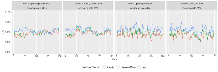
Figure 1: Empirical size (proportion of statistic values greater than $\chi^{2}_{3,0.95}$) calculated at each update using the identity, KM, and log transformations under the null hypothesis. This figure appears in color in the electronic version of this article.

Three choices of $g(t)$ were considered, the identity, KM, and log transformations, in the calculation of the test statistics. For each choice, we calculated both $T_{k}({\boldsymbol{G}})$ and $T_{k}^{w}({\boldsymbol{G}})$ with $w=5$ upon arrival of each block of simulated data. Figure 1 summarizes empirical sizes of the test with nominal level 0.05 at each accumulation point $k=1,\ldots,100$ for the two versions of the tests under two censoring levels. The empirical sizes for the three choices of $g(t)$ fluctuate closely around the nominal level 0.05 in all the scenarios. The log transformation, however, results in a slightly larger size, and its usage should therefore be treated with caution.

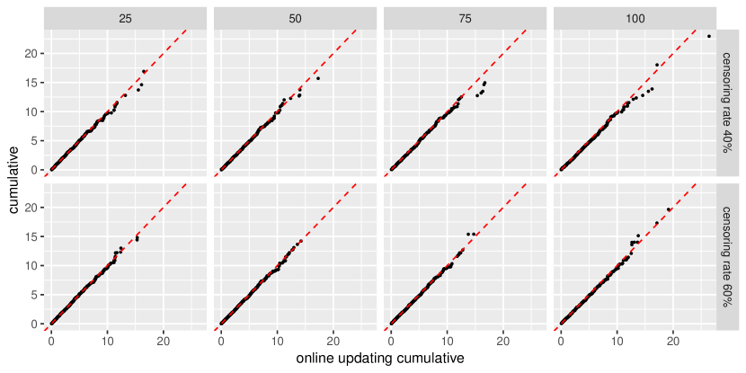
Figure 2: Empirical quantile-quantile plots of the online updating cumulative statistics $T_{k}(G)$ ($x$-axis) and $T_{1:k}(G)$ obtained using cumulative data ($y$-axis) with censoring rate 40% and 60%, taken at block $k\in\{25,50,75,100\}$, both calculated using the KM transformation on event times. This figure appears in color in the electronic version of this article.

To compare the empirical distribution of $T_{k}({\boldsymbol{G}})$ and the standard statistic $T_{1:k}({\boldsymbol{G}})$, we additionally computed $T_{1:k}({\boldsymbol{G}})$ at blocks $k\in\{25,50,75,100\}$ based on cumulative data up to those blocks. Figure 2 presents the quantile-quantile plots of the two statistics obtained with $g(t)$ being the KM transformation. The points line up closely on the 45 degree line, confirming that the online updating cumulative statistics $T_{k}({\boldsymbol{G}})$ follow the same asymptotic $\chi^{2}_{p}$ distribution under the null hypothesis as $T_{1:k}({\boldsymbol{G}})$.

Additional simulation results on the sizes for scenarios where $p\in\{10,20\}$ and where covariate coefficients are piecewise constant with respect to time (and accommodated in the PH model by including additional covariates to handle the pieces separately) are reported in Web Appendices B.3 and B.4. In both cases, the size was well-maintained.

4.2 Power

Continuing with the simulation setting from Section 4.1, two scenarios where the PH assumption is violated were considered to assess the power of the proposed tests.

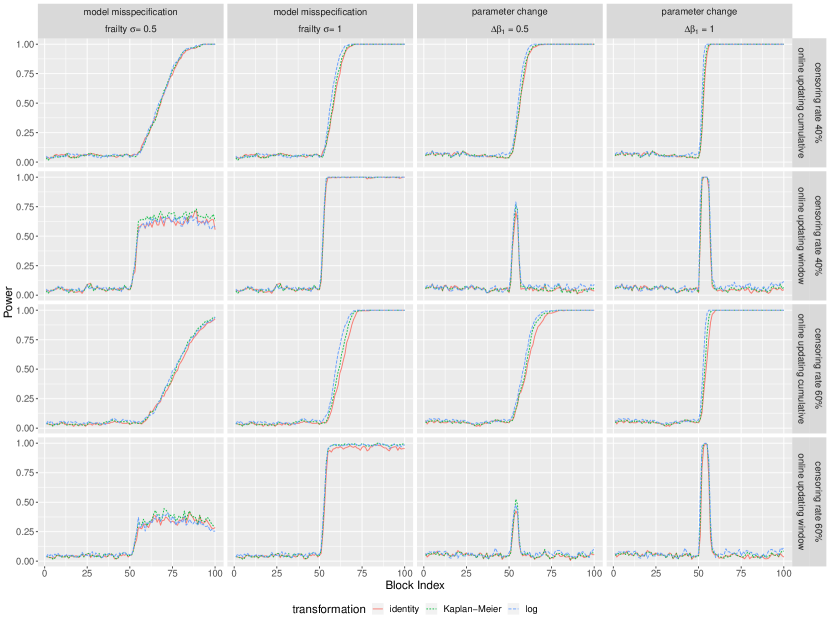
Figure 3: Empirical power (proportion of statistic values greater than $\chi^{2}_{3,0.95}$) for the online updating cumulative and window tests, calculated at each update using the identity, KM, and log transformations under the alternative hypotheses of model misspecification (left) and parameter change (right) under censoring rate $40\%$ (top) and $60\%$ (bottom). This figure appears in color in the electronic version of this article.

The first scenario breaks the PH assumption by a multiplicative frailty in the hazard function. Starting from the 51st block in each stream, the hazard function, instead of being (1), becomes $\lambda_{i}(t)=\lambda_{0}(t)\exp(X_{i}^{\top}{\boldsymbol{\beta}}+\epsilon_{i})$, where a normal frailty $\epsilon_{i}\sim N(0,\sigma^{2})$ is introduced. Two levels of $\sigma$ were considered, 0.5 and 1. Figure 3 shows the empirical rejection rates of the tests at level 0.05 from 1,000 replicates against accumulation point $k$. The tests have higher power under lower censoring rate or higher frailty standard deviation. At a given censoring rate and frailty standard deviation, $T_{k}^{w}({\boldsymbol{G}})$ picks up the change more rapidly than $T_{k}({\boldsymbol{G}})$ because it discards information from older blocks for which the PH assumption holds; the power remains at a certain level (less than 1) after all the blocks in the window contain data generated from the frailty model. While $T_{k}({\boldsymbol{G}})$ responds to the change more slowly, as the proportion of blocks with data generated from the frailty model increases, the power approaches 1 eventually. In all settings, tests based on the log and KM transformations seem to have higher power than that based on the identity transformation.

The second scenario breaks the PH assumption by a change in one of the covariate effects. Specifically, we considered an increase of 0.5 or 1 in $\beta_{1}$, the coefficient for the first covariate in data generation, starting from the 51st block. The empirical rejection rates of the tests with level 0.05 from 1,000 replicates are presented in Figure 3. Both versions of the tests have higher power when the censoring rate is lower or the change in $\beta_{1}$ is larger. At a given censoring rate and change in $\beta_{1}$, $T_{k}^{w}({\boldsymbol{G}})$ only has power to detect the change near the 51st block, where the blocks in the window contain data from two models. The cumulative version, $T_{k}({\boldsymbol{G}})$, picks up the change after the 51st block and the power increases quickly to 1.

A more comprehensive simulation study was conducted to compare the power of $T_{K}({\boldsymbol{G}})$ and the full data test statistic $T({\boldsymbol{G}})=T_{1:K}({\boldsymbol{G}})$ at the end of each data stream, and the results are presented in Web Appendix B.5. When there is a model change, the power of $T_{K}({\boldsymbol{G}})$ is comparable to the power of $T({\boldsymbol{G}})$; when there is a change in covariate effect, $T_{K}({\boldsymbol{G}})$ has significantly higher power than $T({\boldsymbol{G}})$.

5 Survival Analysis of SEER Lymphoma Patients

We consider analyzing the survival time of the lymphoma patients in the SEER program with the proposed methods. Among the 131,960 patients diagnosed with lymphoma between 1973 to 2007, 47,009 experienced an event within 60 months due to lymphoma, resulting in a censoring rate of 64.4%. The risk factors considered in our analysis were Age (centered and scaled), gender indicator (Female), African-American indicator (Black). There were 60,432 females, and 9,199 African-Americans. We wish to compare the performance of the standard statistic $T({\boldsymbol{G}})$ from Equation (6) with $T_{k}({\boldsymbol{G}})$ under a setting in which the PH assumption is judged to be satisfied based on the standard $T({\boldsymbol{G}})$ test. For online updating, the patients in the data were ordered by time of diagnosis, and partitioned by quarter of a year into 140 blocks. The average sample size per block was 943, but the block sizes and censoring rates increased over time; see Web Figure S4.

As a starting point, an initial model that included the three risk factors was fitted, and $T({\boldsymbol{G}})$ based on the full data as in Equation (6) was calculated to be 83.38, which indicated that the model does not satisfy the PH assumption. The online updating cumulative statistic $T_{k}({\boldsymbol{G}})$ was calculated to be 95.60. Due to the relatively high censoring rate, the KM transformation was chosen in calculation of the diagnostic statistics as it is more robust in such a scenario (e.g., Xue and Schifano, 2017). Diagnosis with function plot.cox.zph() in the survival package revealed that all the parameters are likely to be time-dependent; see Web Figure S5.

Techniques in Therneau et al. (2018) were used to allow the parameters to be piecewise-constant over time. Two cut-offs were chosen at 2 and 30 months based on the time-variation pattern of $\widehat{{\boldsymbol{\beta}}}(t)$ obtained from the naive model. A factor variable tgroup is defined to indicate on which intervals the corresponding observation contributes to estimation of ${\boldsymbol{\beta}}$. For example, a subject with survival time 25 and event 1 will now be represented separately on two intervals: one with time interval $(0,2]$, with event 0 and $\textsf{tgroup}=1$, and the other with time interval $(2,25]$, with event 1 and $\textsf{tgroup}=2$. The interaction of Age, Female and Black with the generated tgroup as strata gives the model more flexibility to fit to the data. The new model resulted in $T({\boldsymbol{G}})=T_{1:140}({\boldsymbol{G}})=5.75$ on 9 degrees of freedom with a $p$-value of 0.77, which indicates that the PH assumption for the revised model is appropriate based on the full data. Web Figure S6 presents time-variation plot of parameters for the revised model.

To evaluate the performance of the online updating parameter estimates and test statistics under the revised model, at each block $k,~{}k=1,\ldots,140$, we calculated the parameter estimates, $T_{k}({\boldsymbol{G}})$, $T_{k}^{w}({\boldsymbol{G}})$, and also $T_{1:k}({\boldsymbol{G}})$ based on the single large dataset consisting of all cumulative data up to block $k$. Two versions of $T_{k}({\boldsymbol{G}})$ were obtained, one using the CEE estimator $\widehat{{\boldsymbol{\beta}}}_{k}$ and the other using the CUEE estimator $\widetilde{{\boldsymbol{\beta}}}_{k}$. For $T_{k}^{w}({\boldsymbol{G}})$, the CEE estimator $\widehat{{\boldsymbol{\beta}}}_{k}$ was used as discussed previously, and two widths $w=1$ and $w=10$ were considered. The trajectories of different versions of the test statistics were plotted in the left panel of Figure 4. While the PH assumption seemed to be satisfied within each individual block ($w=1$), as well as in cumulative data up to each accumulation point, both online updating cumulative statistics $T_{k}({\boldsymbol{G}})$ resulted in a rejection of the null hypothesis, and $T_{k}^{w}({\boldsymbol{G}})$ when $w=10$ also resulted in a few rejections along the stream.

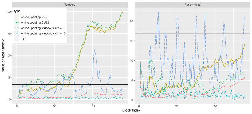
Figure 4: Test statistics for the PH assumption for lymphoma data, using temporally ordered (left) and randomly ordered (right) datasets. This figure appears in color in the electronic version of this article.

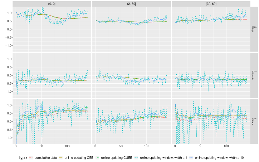
Figure 5: Parameter estimates for Age, Female and Black on intervals $(0,2]$, $(2,30]$ and $(30,60]$, given by different estimating schemes on the temporally ordered lymphoma dataset, plotted against block indices. The decreasing and then increasing trend in the first piece of $\widehat{\beta}_{Age}$ is clear. This figure appears in color in the electronic version of this article.

The trajectories of three parameter estimates $\widehat{\beta}_{\textsf{Age}}$, $\widehat{\beta}_{\textsf{Female}}$, and $\widehat{\beta}_{\textsf{Black}}$ on the three time intervals $(0,2]$, $(2,30]$ and $(30,60]$ (obtained from the covariate interactions with tgroup) were plotted with respect to block indices to investigate this apparent discrepancy; see Figure 5. Apparently, $\widehat{\beta}_{\textsf{Age}}$ on $(0,2]$ remained relatively stable for blocks 1 to 50, but started to first decrease and later increase. This change was captured by both $T_{k}^{w}({\boldsymbol{G}})$ and $T_{k}({\boldsymbol{G}})$, but not by $T_{1:k}({\boldsymbol{G}})$. This is explained by the fact that $T_{1:k}({\boldsymbol{G}})$ is based on a single estimator of ${\boldsymbol{\beta}}$, while in the online updating statistics, each block has its own estimate of ${\boldsymbol{\beta}}$. The temporal changes that are observed in the CUEE estimate of ${\boldsymbol{\beta}}$ get canceled in the calculation based on the full cumulative data.

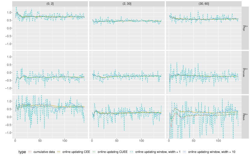
Figure 6: Parameter estimates for Age, Female and Black on intervals $(0,2]$, $(2,30]$ and $(30,60]$, given by different estimating schemes on the randomly ordered lymphoma dataset, plotted against block indices. While the blockwise parameter estimates (window version with $w=1$) are still volatile, there is no significant increasing or decreasing trend from older blocks to newer blocks. This figure appears in color in the electronic version of this article.

To confirm that the temporal change in parameter contributed to the highly significant online updating test statistics, we randomly permuted the order of the observations in the original dataset 1,000 times using the same block size as the original data. For each permutation, we applied the same techniques and cut-offs to allow for piecewise constant parameters over time as before. The histogram of the 1,000 CUEE-based $T_{k}({\boldsymbol{G}})$ is included in Web Figure S7. The empirical $p$-value based on these 1,000 permutations is 0.016, indicating that the particular order of blocks in the original temporally ordered data is indeed contributing to non-proportionality. Figure 6 presents the same diagnostic plots as Figure 5 except that they are for one random permutation. While the final cumulative data parameter estimates remain the same, the trajectories are much flatter, with no obvious temporal trend over blocks. The diagnostic statistics were also obtained under this random permutation, and plotted in the right panel of Figure 4. Each block again satisfies the PH assumption, and the performance of the online updating cumulative statistic based on CUEE is very close to $T({\boldsymbol{G}})$ computed on the entire dataset. The online updating window version ($w=10$), however, still identified a few neighborhoods where the variation is large, and this behavior persists across different choices of window size.

6 Discussion

We developed online updating test statistics for the PH assumption of the Cox model for streams of survival data. The test statistics were inspired by the divide and conquer approach (Lin and Xi, 2011) and the online updating approach for estimation and inference of regression parameters for estimating equations (Schifano et al., 2016). We proposed two versions of test statistics, $T_{k}({\boldsymbol{G}})$ using cumulative information from all historical data, and $T_{k}^{w}({\boldsymbol{G}})$ using information only from more recent data. Both statistics have an asymptotic $\chi^{2}_{p}$ distribution under the null hypothesis. In our simulation studies, the power of $T_{k}({\boldsymbol{G}})$ is comparable to or higher than the power of the standard test $T({\boldsymbol{G}})$ on the entire dataset, for scenarios of a model change or parameter change, respectively. In addition, when $T({\boldsymbol{G}})$ fails to detect violation of the null hypothesis on the whole dataset, $T_{k}({\boldsymbol{G}})$ may still identify the violation with high power. This was observed in our application to the SEER data, and also echoes the findings in Battey et al. (2018). This also suggests that, even when the dataset is not huge, it might be desirable to partition the data and examine the partitions for possibly masked violations of the null hypothesis. At the final block, the cumulative version test statistic will help us decide if the PH assumption has been satisfied. The window version, however, can be run at the same time, as it is sensitive to heterogeneity among a few blocks.

As with previous online updating approaches, $T_{k}({\boldsymbol{G}})$ and $T_{k}^{w}({\boldsymbol{G}})$ are computationally fast, and minimally storage intensive. As shown in the supporting information, the methods are also capable of handling large datasets of a few gigabyte’s size, and can return the estimation and diagnostic results within reasonable time limit. Compared to parallel computing for such datasets, the proposed approach reduces time needed for communication between nodes, and allows for bias correction of the parameter estimates.

A few issues beyond the scope of this paper are worth further investigation. The size of blocks should be chosen following general guidelines (e.g., Schoenfeld, 1983) so that the covariate effects can be sufficiently identified, and that the information matrices exist and are invertible. In practice, with a data stream, we can always choose to let the data accumulate until a certain number of events are observed. Then these observations can be grouped into one block, which can produce stable and valid results for test purposes. For $T_{k}^{w}({\boldsymbol{G}})$, the choice of $w$ may affect the test results and local parameter estimates. Possible influential factors include the size of data chunks, the censoring rate within each chunk, among others. Additionally, as we are more interested in local or current goodness-of-fit when using the window version, $w$ should generally be small. Also, as illustrated in Figure 3, $T_{k}^{w}({\boldsymbol{G}})$ can behave differently under different violations of the PH assumption, therefore, prior knowledge on what types of changes are likely to occur, if available, may also be taken into consideration. As we are more concerned with deciding whether the entire stream satisfies the PH assumption, this window version should be treated as of auxiliary purpose. Also, the test statistics and parameter estimates perform well when $p$ is small to moderate. When $p$ is high or ultra-high, singularity issues could arise, and appropriate penalization methods should be considered (e.g. Fan and Li, 2002; Zou, 2008; Mittal et al., 2014).

Finally, in this work we are only concerned with making a final decision regarding the PH assumption at the end of a data stream. There are scenarios, however, under which we may wish to make decisions alongside the data stream as the updating process progresses. This brings up the issue of multiple hypothesis testing. Hypothesis testing in the online updating framework is an interesting topic, and has been explored recently in Webb and Petitjean (2016) and Javanmard and Montanari (2018), and also in the statistical process control framework in, e.g., Lee and Jun (2010, 2012). Appropriate adjustment procedures in the online updating PH test context are areas devoted for future research.

References

- Air Transport Action Group (2018) Air Transport Action Group (2018). Aviation: Benefits beyond borders (2018) – global summary. https://www.atag.org/component/attachments/attachments.html?id=708. Online; accessed Dec 30, 2018.
- Battey et al. (2018) Battey, H., Fan, J., Liu, H., Lu, J., and Zhu, Z. (2018). Distributed testing and estimation under sparse high dimensional models. The Annals of Statistics 46, 1352–1382.
- Cox (1972) Cox, D. R. (1972). Regression models and life-tables. Journal of the Royal Statistical Society. Series B (Methodological) 34, 187–220.
- Cox (1975) Cox, D. R. (1975). Partial likelihood. Biometrika 62, 269–276.
- Efron (1977) Efron, B. (1977). The efficiency of Cox’s likelihood function for censored data. Journal of the American Statistical Association 72, 557–565.
- Fan and Li (2002) Fan, J. and Li, R. (2002). Variable selection for Cox’s proportional hazards model and frailty model. Annals of Statistics 30, 74–99.
- Fleming and Harrington (1991) Fleming, T. R. and Harrington, D. P. (1991). Counting Processes and Survival Analysis. New York: Wiley.
- Grambsch and Therneau (1994) Grambsch, P. M. and Therneau, T. M. (1994). Proportional hazards tests and diagnostics based on weighted residuals. Biometrika 81, 515–526.
- Javanmard and Montanari (2018) Javanmard, A. and Montanari, A. (2018). Online rules for control of false discovery rate and false discovery exceedance. The Annals of Statistics 46, 526–554.
- Lee and Jun (2010) Lee, S.-H. and Jun, C.-H. (2010). A new control scheme always better than X-bar chart. Communications in Statistics – Theory and Methods 39, 3492–3503.
- Lee and Jun (2012) Lee, S.-H. and Jun, C.-H. (2012). A process monitoring scheme controlling false discovery rate. Communications in Statistics – Simulation and Computation 41, 1912–1920.
- Lin and Xi (2011) Lin, N. and Xi, R. (2011). Aggregated estimating equation estimation. Statistics and its Interface 4, 73–83.
- Mittal et al. (2014) Mittal, S., Madigan, D., Burd, R. S., and Suchard, M. A. (2014). High-dimensional, massive sample-size Cox proportional hazards regression for survival analysis. Biostatistics 15, 207–221.
- National Association of Realtors (2018) National Association of Realtors (2018). Quick real estate statistics. https://www.nar.realtor/research-and-statistics/quick-real-estate-statistics. Online; accessed Dec 30, 2018.
- Schifano et al. (2016) Schifano, E. D., Wu, J., Wang, C., Yan, J., and Chen, M.-H. (2016). Online updating of statistical inference in the big data setting. Technometrics 58, 393–403.
- Schoenfeld (1983) Schoenfeld, D. A. (1983). Sample-size formula for the proportional-hazards regression model. Biometrics 39, 499–503.
- Therneau et al. (2018) Therneau, T., Crowson, C., and Atkinson, E. (2018). Using time dependent covariates and time dependent coefficients in the Cox model.
- Therneau (2015) Therneau, T. M. (2015). A Package for Survival Analysis in S. version 2.38.
- Therneau and Grambsch (2000) Therneau, T. M. and Grambsch, P. M. (2000). Modeling Survival Data: Extending the Cox Model. Springer-Verlag Inc, Berlin; New York.
- Wang et al. (2019) Wang, Y., Palmer, N., Di, Q., Schwartz, J., Kohane, I., and Cai, T. (2019). A fast divide-and-conquer sparse Cox regression. Biostatistics Forthcoming.
- Webb and Petitjean (2016) Webb, G. I. and Petitjean, F. (2016). A multiple test correction for streams and cascades of statistical hypothesis tests. In Proceedings of the 22nd ACM SIGKDD International Conference on Knowledge Discovery and Data Mining, KDD ’16, pages 1255–1264, New York, NY, USA. ACM.
- Xue (2018) Xue, Y. (2018). ys-xue/Code-for-Online-Updating-Proportional -Hazards-Test:First Release.
- Xue and Schifano (2017) Xue, Y. and Schifano, E. D. (2017). Diagnostics for the Cox model. Communications for Statistical Applications and Methods 24, 583–604.
- Zou (2008) Zou, H. (2008). A note on path-based variable selection in the penalized proportional hazards model. Biometrika 95, 241–247.