The JCMT Gould Belt Survey: SCUBA-2 Data-Reduction Methods and Gaussian Source Recovery Analysis

Helen Kirk NRC Herzberg Astronomy and Astrophysics Research Centre, 5071 West Saanich Rd, Victoria, BC, V9E 2E7, Canada Department of Physics and Astronomy, University of Victoria, 3800 Finnerty Road, Victoria, BC, Canada V8P 5C2 Jennifer Hatchell Physics and Astronomy, University of Exeter, Stocker Road, Exeter EX4 4QL, UK Doug Johnstone NRC Herzberg Astronomy and Astrophysics Research Centre, 5071 West Saanich Rd, Victoria, BC, V9E 2E7, Canada Department of Physics and Astronomy, University of Victoria, 3800 Finnerty Road, Victoria, BC, Canada V8P 5C2 David Berry East Asian Observatory, 660 N. A‘ohōkū Place, University Park, Hilo, Hawaii 96720, USA Tim Jenness Joint Astronomy Centre, 660 N. A‘ohōkū Place, University Park, Hilo, Hawaii 96720, USA LSST Project Office, 933 N. Cherry Ave, Tucson, AZ 85719, USA Jane Buckle Astrophysics Group, Cavendish Laboratory, J J Thomson Avenue, Cambridge, CB3 0HE, UK Kavli Institute for Cosmology, Institute of Astronomy, University of Cambridge, Madingley Road, Cambridge, CB3 0HA, UK Steve Mairs East Asian Observatory, 660 N. A‘ohōkū Place, University Park, Hilo, Hawaii 96720, USA Erik Rosolowsky Department of Physics, University of Alberta, Edmonton, AB T6G 2E1, Canada James Di Francesco NRC Herzberg Astronomy and Astrophysics Research Centre, 5071 West Saanich Rd, Victoria, BC, V9E 2E7, Canada Department of Physics and Astronomy, University of Victoria, 3800 Finnerty Road, Victoria, BC, Canada V8P 5C2 Sarah Sadavoy Harvard-Smithsonian Center for Astrophysics, 60 Garden Street, Cambridge, MA 02138, USA Malcolm Currie Joint Astronomy Centre, 660 N. A‘ohōkū Place, University Park, Hilo, Hawaii 96720, USA RAL Space, Rutherford Appleton Laboratory, Harwell Oxford, Didcot, Oxfordshire, OX11 0QX, UK Hannah Broekhoven-Fiene Department of Physics and Astronomy, University of Victoria, 3800 Finnerty Road, Victoria, BC, Canada V8P 5C2 Joseph C. Mottram Leiden Observatory, Leiden University, PO Box 9513, 2300 RA Leiden, The Netherlands Max-Planck Institute for Astronomy, Königstuhl 17, 69117 Heidelberg, Germany Kate Pattle Jeremiah Horrocks Institute, University of Central Lancashire, Preston, Lancashire, PR1 2HE, UK Institute of Astronomy and Department of Physics, National Tsing Hua University, Hsinchu 30013, Taiwan Brenda Matthews NRC Herzberg Astronomy and Astrophysics Research Centre, 5071 West Saanich Rd, Victoria, BC, V9E 2E7, Canada Department of Physics and Astronomy, University of Victoria, 3800 Finnerty Road, Victoria, BC, Canada V8P 5C2 Lewis B. G. Knee NRC Herzberg Astronomy and Astrophysics Research Centre, 5071 West Saanich Rd, Victoria, BC, V9E 2E7, Canada Gerald Moriarty-Schieven NRC Herzberg Astronomy and Astrophysics Research Centre, 5071 West Saanich Rd, Victoria, BC, V9E 2E7, Canada Ana Duarte-Cabral School of Physics and Astronomy, Cardiff University, The Parade, Cardiff, CF24 3AA, UK Sam Tisi Department of Physics and Astronomy, University of Waterloo, Waterloo, Ontario, Canada N2L 3G1 Derek Ward-Thompson Jeremiah Horrocks Institute, University of Central Lancashire, Preston, Lancashire, PR1 2HE, UK

Abstract

The JCMT Gould Belt Survey was one of the first Legacy Surveys with the James Clerk Maxwell Telescope in Hawaii, mapping 47 square degrees of nearby ( $<500$ pc) molecular clouds in both dust continuum emission at 850 $\mu$ m and 450 $\mu$ m, as well as a more-limited area in lines of various CO isotopologues. While molecular clouds and the material that forms stars have structures on many size scales, their larger-scale structures are difficult to observe reliably in the submillimetre regime using ground-based facilities. In this paper, we quantify the extent to which three subsequent data-reduction methods employed by the JCMT GBS accurately recover emission structures of various size scales, in particular, dense cores which are the focus of many GBS science goals. With our current best data-reduction procedure, we expect to recover $100$ % of structures with Gaussian $\sigma$ sizes of $\leq$ 30″ and intensity peaks of at least five times the local noise for isolated peaks of emission. The measured sizes and peak fluxes of these compact structures are reliable (within 15% of the input values), but source recovery and reliability both decrease significantly for larger emission structures and for fainter peaks. Additional factors such as source crowding have not been tested in our analysis. The most recent JCMT GBS data release includes pointing corrections, and we demonstrate that these tend to decrease the sizes and increase the peak intensities of compact sources in our dataset, mostly at a low level (several percent), but occasionally with notable improvement.

^†^†software: Starlink (Currie et al., 2014), CUPID (Berry et al., 2013), KAPPA (Currie & Berry, 2013), SMURF (Jenness et al., 2013; Chapin et al., 2013a), mpfit (Markwardt, 2009), IDL astronomy library, and Coyote Graphics

1 Introduction

The James Clerk Maxwell Telescope (JCMT) Gould Belt Survey (GBS; Ward-Thompson et al., 2007) is one of the initial set of JCMT Legacy Surveys, and has the goal of mapping and characterizing dense star-forming cores and their environments across all molecular clouds within $\sim$ 500 pc. The JCMT GBS included extensive maps of the dust continuum emission at 850 $\mu$ m and 450 $\mu$ m of all nearby molecular clouds observable from Maunakea using SCUBA-2 (Submillimetre Common User Bolometer Array-2; Holland et al., 2013), as well as more-limited spectral-line observations of various CO isotopologues using HARP (Heterodyne Array Receiver Program; Buckle et al., 2009). For this paper, we focus on the SCUBA-2 portion of the survey.

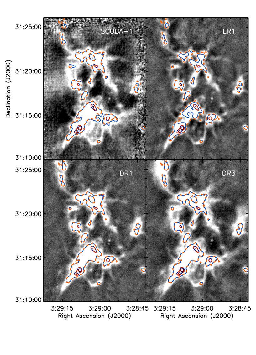
The SCUBA-2 instrument is an efficient and sensitive mapper of thermal emission from cold and compact dusty structures such as dense cores, the birthplace of future stars. One of the science goals of the JCMT GBS is to identify and characterize these dense cores, which includes estimating their sizes and total fluxes (masses). These are challenging observations to make from the ground, as the Earth’s atmosphere is bright and variable at submillimetre wavelengths. As such, all ground-based observations in the submillimetre regime use some form of filtering. Often this filtering is done in the form of ‘chopping’, where fluxes are measured in some differential form (see, e.g. Haig et al., 2004, and references therein). SCUBA-2, however, combines a fast scanning pattern during observing with an iterative filtering technique during the data reduction process, which has the similar consequence of removing both contributions from the atmosphere and extended source emission (e.g., Holland et al., 2013; Chapin et al., 2013b). Regardless of the method, the largest scales of emission cannot be recovered from ground-based submillimetre observations, as it is not possible to disentangle such signal from that of the atmosphere. Nonetheless, it is desirable for star-formation science to obtain accurate measurements of emission structures on as large a scale as possible. New instrumentation, observing techniques, and data-reduction tools allow for better recovery of larger-scale emission structures than was feasible in the past. As an example, Figure 1 shows the emission observed in the NGC 1333 star-forming region in the Perseus molecular cloud as seen with the original SCUBA detector (Sandell & Knee, 2001) compared with the same map obtained with SCUBA-2, as part of the GBS survey, and reduced using several different techniques. The SCUBA-2 map was first presented in Chen et al. (2016) using the GBS Internal Release 1 reduction method, but is shown in Figure 1 using several more recent SCUBA-2 data reduction methods, all of which are discussed further throughout this paper. While bright and compact emission structures appear the same in all panels, the GBS DR3 map clearly recovers the most faint and extended structure, while suffering the least from artificial large-scale features, such as that seen at the centre left of the SCUBA image. In this paper, we focus on the reliability of the GBS SCUBA-2 maps, and do not present any quantitative comparisons with SCUBA data.

While not the focus of our present work, we note that space-based submillimetre facilities such as the Herschel Space Telescope avoid the challenge of observing through the atmosphere, and therefore offer the ability to obtain observations with much less filtering. At the same time, space-based submillimetre facilities have much lower angular resolutions, due to the difficulty in placing large dishes in space. Previous work by JCMT GBS members provide a comparison of star-forming structures observed using Herschel and SCUBA-2 (Sadavoy et al., 2013; Pattle et al., 2015; Ward-Thompson et al., 2016; Chen et al., 2016), although all of these analyses used earlier SCUBA-2 data-reduction methods than the methods analyzed here. The loss of larger-scale emission structures inferred by comparing SCUBA-2 and Herschel observations will therefore be somewhat less severe when the current data products are used instead.

Refer to caption — Figure 1: A comparison of emission observed in NGC 1333. The top left panel shows data from SCUBA, published in Sandell & Knee (2001), while the remaining three panels show SCUBA-2 observations, converted into Jy bm^-1 flux units assuming a 14 $\farcs$ 6 beam as in Dempsey et al. (2013). The SCUBA-2 reductions shown are the JCMT Legacy Release 1 (LR1; top right), JCMT GBS Data Release 1 (DR1; bottom left) and JCMT GBS Data Release 3 (DR3; bottom right), all discussed further in this paper. In all panels, faint emission is emphasized in the grey scale which ranges from -0.05 Jy bm^-1 and 0.1 Jy bm^-1. Both the solid blue and dashed orange contours indicate emission at 0.2 Jy bm^-1, 1 Jy bm^-1, and 3 Jy bm^-1. The solid blue contours trace the greyscale image shown in that panel, while the dashed orange contours show the SCUBA-2 DR3 map for reference.

To achieve the various science goals of the GBS, it is important to have a thorough understanding of the completeness and reliability of the sources detected. Uncertainties in source detection and characterization can arise both from the observations and map reconstruction efforts, as well as from the tools used to identify and characterize the emission sources. In the analysis presented here, we aim to investigate thoroughly the first of these issues, i.e., quantifying how well a source of known brightness and size is recovered in a JCMT GBS map, when an idealized source-detection algorithm is used in an ideal (non-crowded) environment.

The JCMT GBS has released several versions of ever-improving data products to the survey team for analysis: Internal Release 1 (IR1), Data Release 1 (DR1)¹¹1This is called the ‘GBS Legacy Release 1’ in Mairs et al. (2015)., Data Release 2 (DR2), and Data Release 3 (DR3), while the JCMT has also released maps of all data 850 $\mu$ m data obtained between 2011 February 1 and 2013 August 1 through their ‘JCMT Legacy Release 1’ (LR1; Graves et al, in prep; see also http://www.eaobservatory.org/jcmt/science/archive/lr1/). Table 1 summarizes all currently published GBS maps. The last three GBS data releases, intended to be made fully public, are the focus of this paper. We also provide an approximate comparison of the GBS data products to the JCMT’s LR1 maps, which are qualitatively similar to the intermediate ‘automask’ GBS data products discussed in the text.

Within the GBS data releases, DR2 improves on DR1 through the use of improved data-reduction techniques that enhance the ability to recover faithfully large-scale emission structures. Many of these improvements were outlined in Mairs et al. (2015), but it was beyond the scope of that work to replicate fully the data-reduction process used for DR1 and DR2 and quantify how well structure in the maps is recovered. Additionally, several small modifications to the data-reduction procedure were made after the testing performed in Mairs et al. (2015). The majority of this paper focuses on a careful comparison between the recovery of structure using the exact JCMT GBS DR1 and DR2 methodologies. Unlike DR1 and DR2, DR3 does not involve a completely new re-reduction of all JCMT GBS observations with improved recipes. Instead, DR3 focuses on estimating the pointing offset errors present in the observations, and adjusting the final DR2 maps to correct for them.

Table 1: GBS Published Maps^a^aThis table includes only published GBS papers where the submillimetre map was publicly released alongside the paper.

Region	Data Version	Reference	DOI^b^bDigital Object Identifier is a permanent webpage where a static version of the GBS data is stored for public distribution.
CrA	DR1	Bresnahan et al (in prep)	pending
Auriga	DR1	Broekhoven-Fiene et al. (2018)	https://doi.org/10.11570/17.0008
IC5146	DR1	Johnstone et al. (2017)	https://doi.org/10.11570/17.0001
Lupus	DR1	Mowat et al. (2017)	https://doi.org/10.11570/17.0002
Cepheus	DR1	Pattle et al. (2017)	https://doi.org/10.11570/16.0002
Orion A	DR1 automask	Lane et al. (2016)	https://doi.org/10.11570/16.0008
Taurus L1495	IR1	Ward-Thompson et al. (2016)	https://doi.org/10.11570/16.0002
Orion A^c^cWhile analysis was performed only in the southern portion of the map, the entire map is provided at the DOI.	DR1	Mairs et al. (2016)	https://doi.org/10.11570/16.0007
Perseus	IR1	Chen et al. (2016)	https://doi.org/10.11570/16.0004
Serpens W40	DR1	Rumble et al. (2016)	https://doi.org/10.11570/16.0006
Orion B	DR1	Kirk et al. (2016)	https://doi.org/10.11570/16.0003
Ophiuchus	IR1	Pattle et al. (2015)	https://doi.org/10.11570/15.0001
Serpens MWC297	IR1	Rumble et al. (2015)	https://doi.org/10.11570/15.0002

Quantifying the quality and fidelity of our JCMT GBS maps is a crucial step for the over-arching science goals of the survey. For example, one goal is to measure the distribution of core masses and compare this distribution with the initial (stellar) mass function (Ward-Thompson et al., 2007). Without detailed knowledge of source recoverability and whether or not there is any bias in real versus observable flux, the obtained core mass function could be misinterpreted. A wide range of artificial Gaussians were used in our testing, ranging from sources that should be difficult to detect (e.g., peak brightnesses similar to the image noise level) to those that should be easy to recover accurately (e.g., compact sources with peaks at 50 times the image noise level). We emphasize that especially for the former case, the recovery results we present here represent an unachievable ideal case for realistic analysis: knowing precisely where to look for the injected peaks, as well as precisely what to look for (known peak brightness and width) allows us to recover sources that would never be identifiable in a real observation. A full quantification of completeness would require including non-Gaussian sources (e.g., also filamentary morphologies, and elongated cores with non-Gaussian radial profiles), testing the effects of source crowding, testing several of the commonly used source-finding algorithms and determining the influence of false positive detections, and not tuning the source-finding algorithm to look for emission in known locations. Such an analysis is beyond the scope of this paper, although some aspects have been examined by previous studies (e.g., Rosolowsky et al., 2008; Pineda et al., 2009; Kainulainen et al., 2009; Kauffmann et al., 2010; Shetty et al., 2010; Rosolowsky et al., 2010; Reid et al., 2010; Ward et al., 2012; Men’shchikov, 2013).

The paper is structured as follows. In Section 2, we discuss the JCMT GBS observations and the general data-reduction procedure. In Section 3, we describe our method for testing source recoverability and fidelity in source recovery in the DR1 and DR2 maps, and the results are discussed in Section 4. These tests provide essential metrics for future analyses of GBS data where the role of bias and the recoverability of real structure in the observations will need to be understood. In Section 5, we introduce two independent methods for measuring the telescope-pointing errors in each observation, and demonstrate that the final DR3 maps should have little residual relative pointing error. This analysis provides us with confidence that the properties of emission structures measured in DR3 should not be substantially more blurred out than expected from the native telescope resolution.

2 Observations

SCUBA-2 observations were obtained between 2011 October 18 and 2015 January 26. Observations were made in Grade 1 ( $\tau_{\mathrm{225GHz}}<0.05$ ) and Grade 2 ( $0.05<\tau_{\mathrm{225GHz}}<0.08$ ) weather conditions. Grade 1 weather provides good measurements at both 850 $\mu$ m and 450 $\mu$ m, while Grade 2 weather is suitable for 850 $\mu$ m and provides poorer measurements at 450 $\mu$ m. Each field was observed four to six times depending on the local weather conditions, to obtain approximately constant noise levels across the survey at 850 $\mu$ m. Observations at 450 $\mu$ m are more sensitive to the atmospheric conditions, and hence show a significantly larger variation in noise properties.

Table 4 summarizes the approximate noise level in each field of the survey, while Figure 2 shows the distribution of noise levels. We ran the Starlink Picard (Gibb et al., 2013) recipe mapstats on each individual observation to calculate the noise in the central portion (i.e., inner circle of radius 90″) of the observed area. We then estimated the effective noise for each field in the final mosaic by accounting for the fact that the observations are combined using the mean values weighted by the inverse square of the noise at that location. For most of the paper, we focus on the 850 $\mu$ m data, where the noise levels are more uniform.

The standard observing mode used for the GBS data was the PONG 1800 mode (Kackley et al., 2010), which produces fully sampled 30′ diameter regions. The GBS obtained a total of 581 observations under this mode, as well as a handful of additional observations under the PONG 900 and PONG 3600 modes during SCUBA-2 science verification (SV). We focus our analysis here entirely on the PONG 1800 observations. Earlier testing by the GBS data-reduction team showed that the other mapping modes have different sensitivities to large-scale structures.

We reduced the maps using the iterative routine known as makemap, which is distributed as part of the smurf package (Chapin et al., 2013b, a) in Starlink (Currie et al., 2014). We used a gridding size of 3″ pixels at 850 $\mu$ m and 2″ pixels at 450 $\mu$ m, and halted iterations when the map pixels changed on average by $<0.1$ % of the estimated map rms. In both DR1 and DR2, we reduced each observation twice, following a similar overall procedure. In the first reduction, known as the automask reduction, pixels containing real astronomical signal were estimated using various signal-to-noise ratio (SNR) criteria applied to the raw data time stream. We then mosaicked together all maps of the same region, and determined more comprehensive areas of likely real astronomical signal. These areas were then supplied as a mask for the second round of individual reductions known as the external-mask reduction. The final mosaic was created using the output of the second round of reductions.

The final (external mask) mosaic tends to contain much more large-scale emission structure than is in the first (automask) mosaic. The reason for this difference is that the map-making algorithm needs to distinguish between larger modes of variation in the raw time stream data, which arise from scanning across true astronomical signals, versus those induced by variations in the sky or instrumental effects, which it does through the use of a mask. By being able to combine four to six initially reduced maps together to determine where real astronomical signal is likely, it is possible to identify accurately emission over a much larger area of sky than is evident from the raw data in a single observation. The differences between our DR1 and DR2 procedures focused on methods of improving the sensitivity to larger-scale structure in the initial automask reduction (e.g., reducing large-scale filtering), as well as creating more generous, but still accurate, masks for the external-mask reduction (e.g., lowering the mask SNR criteria). We note that in defining the mask, there are two competing challenges, as also discussed in Mairs et al. (2015). Masks that are smaller than the true extent of the source emission will prevent a full recovery of that emission, leading to artificially smaller and fainter sources. At the same time, masks that include regions without real source emission are liable to introduce false large-scale structure which may artificially increase the total size and brightness of real sources. Appendix A outlines the full reduction procedure and makemap parameters applied for both DR1 and DR2.

Although not identical, the data-reduction procedure for the JCMT’s Legacy Release 1 (LR1) dataset is similar to the GBS DR1 automask procedure: only one round of reduction is run, and strong spatial filtering is applied to suppress real and artificial large-scale structures.

In DR3, we use the DR2 reductions for each observation, and then search for possible offsets between observations of the same field due to telescope-pointing errors. If positional offsets are found, we apply the appropriate shift to the observation before creating the final mosaicked image. This procedure is discussed in more detail in Section 5.

One final data-reduction parameter which we do not refine beyond the standard recommended procedure is the appropriate flux conversion factor applied to each observation. As discussed in Dempsey et al. (2013), the standard observatory-derived FCF values appear stable over time, with a scatter of less than 5% at 850 $\mu$ m and about 10% at 450 $\mu$ m in relative calibration, while the absolute calibration factors are approximately 8% and 12% at 850 $\mu$ m and 450 $\mu$ m, respectively. The JCMT Transient Survey demonstrates that it is possible to improve the relative calibration at 850 $\mu$ m to 2%-3% (Mairs et al., 2017a), however, the Transient Survey procedure requires multiple bright point sources per observation, which many GBS fields do not possess. We therefore simply note that the GBS source flux estimates should be accurate to 8% at 850 $\mu$ m and 12% at 450 $\mu$ m using the default calibrations, as confirmed in Mairs et al. (2017a). A small fraction of sources may also have variable emission, although most of the variable candidates identified in the Transient Survey show variations in flux of less than a few percent over the course of the typically short (days or months) time span between typical GBS observations of the same field (Mairs et al., 2017b; Johnstone et al., 2018). Only one source of the $\sim$ 150 monitored by the Transient Survey shows variability of more than 10% over short time scales (EC 53 in Serpens Yoo et al., 2017; Johnstone et al., 2018).

For completeness, we note that where available, all GBS data releases additionally include ‘CO-subtracted’ maps. The ¹²CO(3-2) emission line lies within the 850 $\mu$ m bandpass, and therefore can contribute flux to the emission measured (e.g., Drabek et al., 2012). This ‘CO contamination’ is typically $<10$ % of the total flux measured, although it can be significantly higher (up to 80%) in rare cases where there is an outflow in a lower density environment. Where appropriate measurements of the ¹²CO(3-2) integrated intensity were available to the GBS, we ran an additional round of reductions for each of DR1, DR2, and DR3 with the CO emission properly subtracted from the 850 $\mu$ m map. A brief summary of our CO subtraction procedure is given in Appendix A.4.

3 Source Recovery Measurements

Here, we discuss our procedure for measuring our accuracy in recovering emission structures.

3.1 Test Setup

As discussed in Section 2, Starlink’s makemap is the standard software for reducing SCUBA-2 mapping observations. Using makemap, the user can insert artificial sources directly into an observation’s raw-data time stream, providing an easy mechanism to measure how well idealized model emission structures are recovered under different data-reduction settings. Our approach was guided by the aim to test systematically the best-case scenario of isolated point sources that are not confused by a local background. We emphasize that many of the dense cores identified in the GBS will have some degree of crowding and / or hierarchical structures, which will reduce the reliability of the recovered emission. We used the GBS 850 $\mu$ m observations of the OphScoN6 field as the basis for our testing. It is the GBS field that contains the least amount of real signal, i.e., the observation mostly closely resembling a pure-noise field. OphScoN6 was observed seven times rather than the standard six times for observations obtained in Grade 2 weather, so we excluded one of the observations (20130702_00031) to make the dataset more similar to a standard GBS field. This excluded observation was taken under marginal weather conditions with higher noise levels than is typical for most GBS observations. The noise at 850 $\mu$ m in the mosaic of the six OphScoN6 maps is 0.049 mJy arcsec^-2, which is similar to those of other GBS fields (cf. Table 4 and Figure 2).

Figure 3 shows the DR2 automask reduction of the OphScoN6 data used here. A careful visual examination of the map shows that there are two faint zones of potentially real emission to the east of the field but, with the low peak signal level, neither are definite detections. Nonetheless, we take care in our completeness testing to avoid potential biases due to low-level emission in these regions.

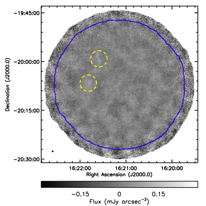
We generate artificial, radially-symmetric Gaussian sources with a range of peak intensities and widths to add to each raw observation, to test how well they are recovered in the final reduced mosaic. We constrained all fake sources to lie in angular separation at least 3 Gaussian $\sigma$ away from the outer 3′ of the map (where the local noise is significantly higher), and also away from the zone of potential emission in the east of the mosaic, defined as two circles of 2.5′ radius, with the centres set by eye. Both of these excluded map areas are shown in Figure 3.

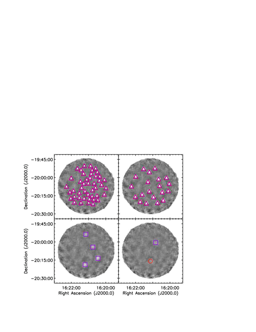
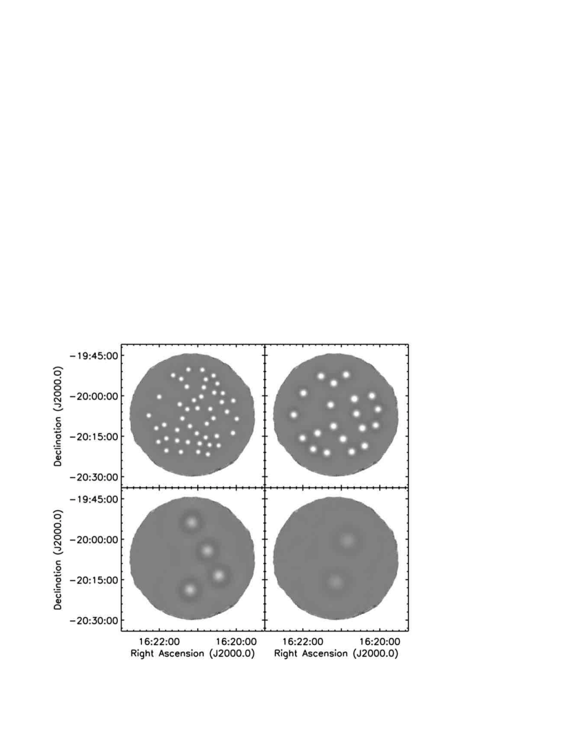
For any given set of Gaussian parameters (i.e., amplitude and width), we randomly placed 500 sources, eliminating those which landed in the edge or possible emission zones noted above, or those located less than 6 $\sigma$ away from a previously placed source. In the case of the narrowest ( $\sigma=$ 10″) Gaussians we tested, this process resulted in more than 100 inserted sources per map. For the widest ( $\sigma=$ 150″) Gaussians that we tested, however, only one or two sources could be placed in a map while still satisfying all of the above criteria. We therefore created multiple maps with artificial sources added for the widest Gaussians to improve our statistics. We note, however, that our statistics are still poorer for the widest Gaussian cases. It is too computationally intensive to run hundreds of reductions for each wide Gaussian to match the number of sources able to be inserted in a single narrow Gaussian test image²²2For reference, the reduction of each SCUBA-2 raw observation requires approximately 1.5 hours running on a dedicated 100 GB RAM, 12 core CPU machine, while each test Gaussian input field uses a mosaic of six raw observations, and requires four reductions (DR1 and DR2, automask and external mask).. Table 2 summarizes the Gaussian parameters used for testing, and lists the total number of artificial sources used for each combination of width and peak. In total, we inserted 3196 artificial Gaussian sources into the maps. We explored 63 different Gaussian widths and amplitudes, with a total of 306 test fields, to boost our statistics.

Figure 4 shows an example of the test setup, with the artificial Gaussian sources added directly to the original mosaic. Since these Gaussians have not passed through our data-reduction pipeline, deviations from perfect Gaussians are entirely attributable to the background noise in the mosaic.

Table 2: Number of Gaussian Peaks Analyzed

Amplitude	Sigma (arcsec)
( $N_{\mathrm{rms}}$ )	10	30	50	75	100	125	150
1	163	50	57	36	24	14	10
2	170	45	61	37	21	20	11
3	151	52	63	37	23	16	9
5	171	48	55	42	22	19	9
7	147	53	53	37	24	20	9
10	181	45	57	37	21	16	12
15	159	45	58	34	20	19	11
20	166	48	57	35	20	15	11
50	152	52	58	37	23	17	11
N_repeat^a^aThe number of reductions run for each input Gaussian sigma value, done to increase the total number of artificial sources available for analysis.	1	1	3	5	6	9	9

3.2 Data Reduction

After creating each instance of artificial Gaussians, we run our standard GBS data-reduction procedure with the artificial Gaussians added directly into the raw-data time stream for each of the six observations of OphScoN6 using the ‘fakemap’ parameter in makemap. The standard reduction procedure is outlined in Section 2. We emphasize that the external mask is created separately for each set of artificial Gaussians, based on the individual automask reductions. We follow these steps for both the DR1 and DR2 reduction procedures. For each set of added artificial Gaussians, we therefore have four maps to examine: DR1 and DR2, automask and external-mask reductions. Figure 5 shows the DR2 external-mask reductions for the four test cases from Figure 4. Comparison of these two figures reveals a clear difference in the quality of source recovery for smaller and larger sources, which will be analyzed quantitatively in Section 4.

3.3 Source Recovery

We next use an automated method to determine how well the artificial Gaussians are recovered in each of the maps. In normal scientific analyses, uncertainties in where real emission is located and its true structure can complicate emission recovery. Here, we take advantage of knowing precisely where the emission is located and what the brightness profile should look like to reduce the uncertainties associated with source recovery. For each known artificial Gaussian peak position, we use mpfit (Markwardt, 2009) to search the surrounding 3.0 $\sigma$ radius for a given input Gaussian size. This search window is large enough to encompass the model Gaussian peak to 0.003 times the peak brightness, which corresponds to about one tenth of the image rms for the brightest model Gaussians. To eliminate spurious noise features being identified, we discard any fits that did not converge, had large fitting uncertainties³³3 Specifically, we discarded fits where the ratio of the peak flux or width and its associated fitting error was less than three, i.e., any fits where the peak flux or width was uncertain by at least 100% within the standard 3-sigma uncertainty range. We also excluded fits where the uncertainty in the location of the peak exceeded 50% of the input Gaussian width., were dominated by an artificial background term⁴⁴4Small fitted background terms may be reasonable if the source lies near the peak or valley of a noise feature in the mosaic. We excluded fits where the absolute background exceeded half of the input peak flux or one third of the fitted peak flux., or had properties too different from the input values⁵⁵5This criterion required true source recoveries to have a peak location within 1.25 $\sigma$ of the true centre – a radius of 1.25 $\sigma$ corresponds roughly to the full width at half maximum, or FWHM. We also required the fits to be approximately round (axial ratios less than 1.5), to have a peak no more than 2.5 times the real value, and to have a width no more than twice the real value. Finally, we excluded fits which were offset from their input locations by more than the input Gaussian width divided by the square root of the peak signal-to-noise of the input Gaussian; brighter Gaussians should have more accurately determined centres.. We did not eliminate sources which were much fainter or smaller than the input Gaussians, as we expect the data-reduction process to create smaller and fainter sources than we started with, as shown by Mairs et al. (2015) and we wish to quantify this effect. Finally, to ensure that noise spikes or underlying larger-scale structure from the original data were not contaminating our results, we performed a similar Gaussian fit on the original mosaics (i.e., maps with no artificial sources added). We then removed from our list of recovered artificial sources any fits which had consistent fit parameters to the original mosaic fit (within 1.5 times the fit uncertainty in all fit parameters). We emphasize that our entire Gaussian-fitting procedure gives the best case possible for source recovery. Many of the faintest sources that we can find in our maps would not be identifiable using a standard source-detection algorithm that was not targeted to known positions and Gaussian properties.

We note that all of our source recovery tests discussed here and in the following sections focus on the 850 $\mu$ m observations. We expect that the 450 $\mu$ m data would follow qualitatively similar trends, but would not behave identically. Early testing by the data reduction team showed that in general, large-scale structure is better recovered when larger pixel sizes are adopted. The GBS uses smaller pixels for the 450 $\mu$ m maps (2″) than the 850 $\mu$ m maps (3″) to account for the smaller beamsize of the former. Therefore, we expect that for structures of equal size and the same peak brightnesses signal to noise ratios, recovery will be poorer in the 450 $\mu$ m map⁶⁶6Source recovery testing at 450 $\mu$ m is also complicated by the fact that we apply the 850 $\mu$ m-based mask for the 450 $\mu$ m data reduction..

4 Analysis: Artificial Source Recovery

In our analysis below, we examine the final reduced mosaics to determine the effectiveness of each reduction in recovering the artificial Gaussians introduced into the raw-data time stream. The quantitative metrics that we examine are the fraction of Gaussians recovered, as well as the recovered peak flux, total flux, and size compared with the input values, as well the recovered axial ratio and offsets in the recovered peak position. We also note that our artificial source recovery also gives us a tool not available for normal observations. By comparing the reduced maps with and without the artificial sources added to the raw-data time stream, we can measure precisely how much flux each artificial source contributes to the final reduced map. The analysis of the difference maps is presented in Appendix B.

4.1 Recovery Rate

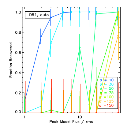
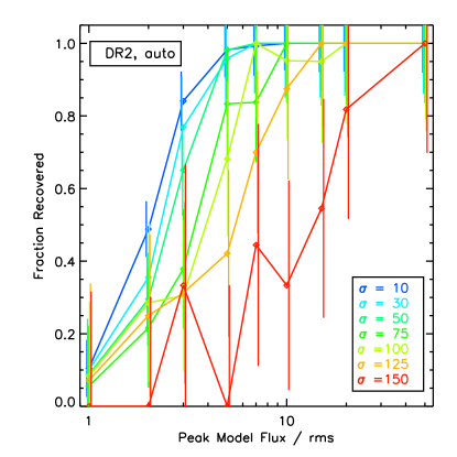
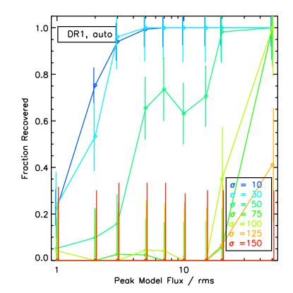
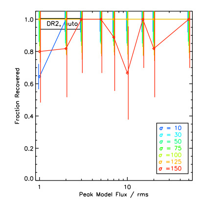
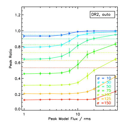
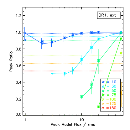
The first metric that we analyze is the recoverability of the artificial Gaussians in the final maps. We emphasize that this recovery rate is an upper limit to the detection rate that would be possible to measure in real observations, where source properties are not known and complications such as source crowding exist. Figure 6 shows the fraction of sources recovered versus the peak flux for Gaussians of various widths using different data-reduction methods. Bright and compact sources are always recovered, regardless of the reduction method. Compact sources become poorly recovered only at extremely low intensity levels, i.e., peak amplitudes of one or two times the mosaic rms. On the other hand, extended sources are more difficult to recover. We also examine the subset of recovered sources that lie within the mask, whose properties are expected to be better recovered (in the external-mask reduction), as demonstrated in Mairs et al. (2015). Some of the recovered sources are only marginally brighter than the local noise level, and in many of these cases, are sufficiently faint that they did not satisfy the masking criteria we adopted. Therefore, we find that the total source recovery rate is poorer for sources which lie within the mask, although it follows the same general trend as the full set of recovered sources (i.e., a higher recovery rate for brighter and more compact input Gaussians). The recovery rate of sources which lie within a mask is generally a better representation of the detection rate of sources which could be confidently identified in real observations, however, an important exception is that moderately bright but very compact sources may have too few pixels to satisfy the DR2 masking criteria, even though they are clearly detectable. A comparison of the DR1 (left column) and DR2 (right column) reductions in Figure 6 shows that the latter is much better at retaining larger sources in the automask and external-mask reductions. For large ( $\sigma\geq 100$ ″) and bright (input peaks $\geq 10\times$ rms) input Gaussians, we typically recover at least twice as many of the Gaussians in DR2 maps as we can in DR1 maps.

In Figure 6, we also see slight improvement in the fraction of recovered sources between the automask and external-mask reductions. We generally expect the external-mask reductions to improve the reliability of recovered source properties (as examined in the following sections), rather than the recovery fraction itself. Indeed, for a source to be included in the external mask, by definition it must be visible already in the automask reduction. Therefore, the similarity in source recovery fractions between automask and external-mask reductions is expected. We attribute the marginal difference in recovered sources in the external-mask reduction to added sources near our detection limit and do not consider the difference in source recoveries to be significant. These faint or extended Gaussians are barely distinguishable from the background-map noise, even with our generous recovery criteria. As also noted in Mairs et al. (2015), the recovery rate for sources in the GBS DR1 map should therefore be similar to the JCMT LR1 maps, which are similar to the GBS DR1 automask reductions.

Our source recovery rates compare favourably with the JCMT Galactic Plane Survey (JPS), a JCMT Legacy Survey which focussed on mapping 850 $\mu$ m emission of large areas of the Galactic Plane using the larger PONG3600 mapping mode. Eden et al. (2017) ran a series of completeness tests injecting artificial Gaussians of FWHM = 21″ ( $\sigma\sim 9$ ″) with a range of peak brightnesses, using the CUPID source detection algorithm FellWalker to measure their observable properties. They report a 90% to 95% detection rate for sources with peak fluxes of 5 or more times the noise level, and did not test the detection rate for larger sources. For comparison, we recover 100% of the $\sigma=10$ ″ sources with peak fluxes of 5 or more times the noise in both external mask reductions.

Table 3 summarizes the percentage of sources recovered in each of the external-mask reductions, as a function of data-reduction method and input artificial Gaussian parameters. In Table 3, the left hand portion of the table provides statistics for all recovered sources, while the right hand portion provides statistics for the subset of recovered sources within an external mask. We again emphasize that these values represent upper limits to the observable detection rate, where a blind search is run on sources with varying levels of crowding.

Table 3: Source Recovery for External Mask Reductions

		Percentage of Sources Recovered (%)
DR Method	$\sigma$ ^a^aThe Gaussian width, sigma, of the inserted artificial Gaussians.	Peak-all ( $N_{\mathrm{rms}}$ )^b^bThe peak flux of the inserted artificial Gaussians, given in units of the rms noise of the map. The source recovery fractions listed in these columns give all of the recoveries within the map.									Peak-mask ( $N_{\mathrm{rms}}$ )^c^cThe peak flux of the inserted artificial Gaussians, given in units of the rms noise of the map. The source recovery fractions listed in these columns give only the recoveries that lie within the external mask.
	(″)	1	2	3	5	7	10	15	20	50	1	2	3	5	7	10	15	20	50
DR1	10	14	78	96	100	100	100	100	100	100	1	24	51	87	98	100	100	100	100
DR1	30	2	11	90	100	100	100	100	100	100	0	2	9	29	47	77	100	100	100
DR1	50	1	0	0	27	81	96	98	100	100	0	0	0	1	13	12	51	94	100
DR1	75	0	0	0	0	0	0	0	68	100	0	0	0	0	0	0	0	14	100
DR1	100	0	0	0	0	0	0	0	0	100	0	0	0	0	0	0	0	0	100
DR1	125	0	0	0	0	0	0	0	0	76	0	0	0	0	0	0	0	0	52
DR1	150	0	0	0	0	0	0	0	0	0	0	0	0	0	0	0	0	0	0
DR2	10	10	58	88	98	100	100	100	100	100	0	0	0	38	87	98	100	100	100
DR2	30	10	35	75	97	100	100	100	100	100	0	0	5	43	98	100	100	100	100
DR2	50	7	29	63	98	100	100	100	100	100	0	0	0	36	73	100	100	100	100
DR2	75	8	24	32	80	83	100	100	100	100	0	0	0	2	29	86	100	100	100
DR2	100	4	28	30	72	95	95	95	100	100	0	0	0	0	4	19	95	100	100
DR2	125	14	20	25	42	70	87	100	100	100	0	0	0	0	0	0	26	66	100
DR2	150	0	0	22	0	55	33	45	81	100	0	0	0	0	0	0	0	9	100

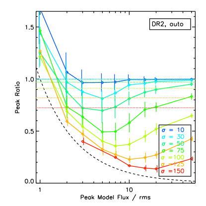
4.2 Recovered Properties: Peak Flux

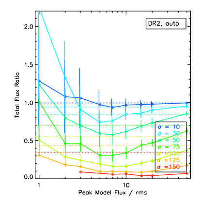
For the artificial Gaussians which were recovered, we now examine how well their measured properties match the input properties. We measure the mean and standard deviation of the recovered Gaussian fit values and compare them to the input Gaussian values. Table 5 summarizes the recovered Gaussian properties for each of the external-mask reductions. For each reduced map, we report on the mean and standard deviation of the fraction of the measured Gaussian property with the initial input value. Table 5 includes the peak flux (discussed here), as well as the Gaussian width $\sigma$ and the total flux (discussed in the following sections).

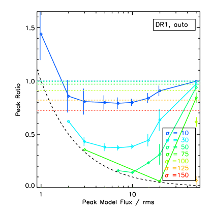
Figure 7 shows how well the peak flux is recovered for all recovered sources. For the faintest input Gaussians, the recovered peak flux is typically larger than the input value, i.e., the peak-flux ratio is above one. Faint artificial sources with peak fluxes near the typical noise level in the map (one or two times the rms) are easier to recover when these sources are coincident with positive noise features in the map. We therefore expect the recovered faintest peaks to have peak fluxes biased towards higher values. Eden et al. (2017) report a similar behaviour for their completeness testing in the JPS maps. The black dashed curve in Figure 7 shows the approximate effect of this bias by showing a measurement of a peak flux equal to the local rms. While not identical, the shape of this curve gives a reasonable approximation of the measured peak flux ratios at low input peak flux values for DR2.

Figure 7 also shows that the peak fluxes are better recovered for compact sources than larger sources. Larger sources have a great fraction of their flux at larger size scales, and are thus expected to be more sensitive to filtering. We constructed a simple model of the large-scale spatial filtering that occurs during data reduction to see how well it predicts the observed source recovery behaviour. Accordingly, we created a series of two-dimensional Gaussian models matching our artificial Gaussian sources. We approximate the filtering as a single-scale boxcar smoothed version of the model being subtracted from the original. We fit the resulting filtered model with a two-dimensional Gaussian (including a constant zero-point term to alleviate fitting challenges with slight negative bowling) to calculate the fractional reduction in peak flux and size.

Previous tests of the initial data-reduction method employed by the GBS (IR1, not examined here) suggested that source recovery was consistent with a simple single filtering scale of about 1′. The subsequent data-reduction methods examined here (DR1 and DR2) were expected to recover more emission, i.e., be described by a larger filtering scale. Our test results confirm the larger scale of filtering, although we also find that a single filter scale is insufficient to describe the recovered source properties for the full range of artificial Gaussians tested. Figure 7 shows the predictions for recovered peak-flux ratio for a filter scale of 600″ (dotted horizontal lines). This filter scale is equal to the large-scale filtering formally applied during data reduction, via the flt.filt_edge_largescale=600 parameter. Peak-flux ratios lying below the model line imply they have been subject to more filtering than in the model, i.e., filtering on a smaller size scale. The 600″ filtering scale matches the smallest artificial Gaussian sources, of sizes of below about 75″ for the external-mask reduction of DR2 – i.e., the dashed filtering model curves are a good match for the recovered peak flux ratios at the highest SNR values. At the same time, the model clearly under-predicts the amount of filtering for larger sources for that same reduction.

Comparing the reductions, Figure 7 clearly shows that DR2 recovers more reliable peak flux values than DR1. Also, although the difference is subtle, the external-mask reductions improve on the automask reductions, especially for the largest and brightest of input Gaussians. In cases where not all of the recovered sources lie within the external mask, the subset of sources that are included in the mask tend to have recovered peak fluxes which more closely correspond to the input value than the full sample of sources do. As an example, in DR2, a Gaussian with $\sigma$ =100″ and a peak flux of 10 times the noise has recovered peak fluxes of about 37% of their true value in the automask reduction, while this rises to roughly 40% of their true value in the external-mask reduction for all sources, and 43% for those lying within the mask. In contrast, no sources are reliably recovered in either the automask or external-mask reduction of DR1 for these Gaussian properties. As noted in Mairs et al. (2015), sources are only accurately recovered in the external-mask reductions when the mask encompasses the true extent of the source. The superiority of the DR2 reductions over the DR1 reductions is therefore partly attributable to the mask-making procedures, which better reflect the true source extents in DR2 than in DR1.

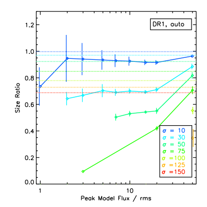
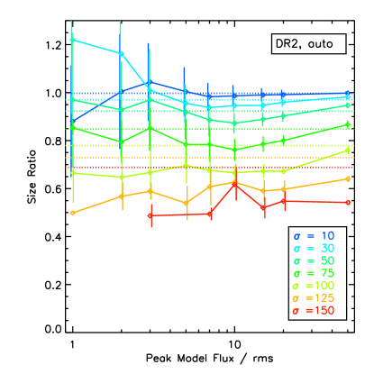
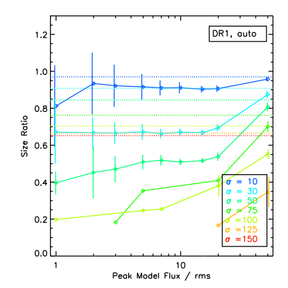
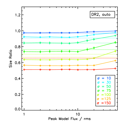
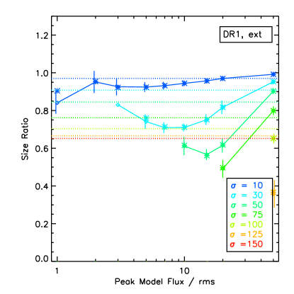
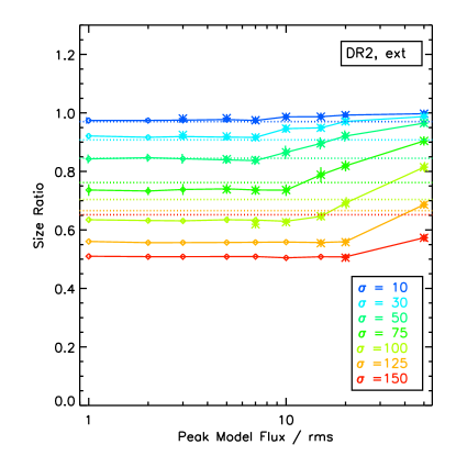
4.3 Recovered Properties: Sizes

Figure 8 shows the size ratios measured for the artificial Gaussians. We remind the reader that the input Gaussians were all round, though we allowed fits for sources with axial ratios up to 1.5:1 (Section 3.3). We present here a single size estimate based on the geometric mean of the two Gaussian $\sigma$ values. In general, we find similar results to those previously presented: (1) compact and brighter Gaussians have their sizes recovered more accurately, (2) DR2 tends to show more reliable structures than DR1, and (3) the external-mask reduction is an improvement over the automask reduction, particularly for sources which lie within a masked area. Using a single size to describe the recovered sources is reasonable, as they tend to be quite round, with mean axial ratios of no more than $\sim$ 1.4:1 for any of the reductions. For sources that are bright or recovered within a mask (or both), the mean axial ratio is almost always lower than 1.2:1, and the sources recovered in the DR2 reduction furthermore tend to have lower axial ratios than those in the corresponding DR1 reduction.

As in Figure 7, we also consider the effects of filtering on the model Gaussians. The dashed lines in Figure 8 shows the ratio of the mean measured filtered size to the input size for the grid of model Gaussians with which we applied a 600″ filter (see previous section for details). As expected, these models show that the more-extended model Gaussians have a greater reduction in size than their more compact counterparts. The filtering model predicts approximately the size ratio for sources smaller than 50″ (blue points and lines), but under-predicts the amount of filtering for the largest sources (i.e., predicts size ratios which are too large).

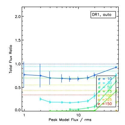
4.4 Total Flux

Here, we present results for the total flux recovered. For individual recovered cores, the trends discussed in the previous two sections (for peak flux and size) are at work. Figure 9 shows the total flux recovered. The values shown in this plot and Table 5 should be considered when analyzing dense core mass functions in GBS data. For compact sources ( $\sigma\leq 30$ ″) which are brighter than 3 times the local noise, the total fluxes are recovered to better than 25% in DR2.

4.5 Location

We also examined the positional offset of the centre of the recovered Gaussian compared with their true input location (not shown). Since the central location is expected to become less certain as the input Gaussian becomes larger, we measured the ratio of the positional offset to the input Gaussian width, $\sigma$ . Using this measure, we find that the offset ratios are typically small, with mean values of 0.3, i.e., offsets of no more than 30% of $\sigma$ , with significantly lower values obtained for model peaks of 10 or more times the rms. For the DR2 external-mask reductions, for cases where the model peak is 10 or more times the rms, the mean offset ratio is $\leq$ 0.05 for all input $\sigma$ . For $\sigma=30$ ″, this implies a typical positional accuracy of better than 1 $\farcs$ 5. We therefore find that the data-reduction and source-recovery processes do not typically induce significant shifts to the true source positions.

4.6 Summary

Our artificial-source recovery tests confirm that the GBS maps more reliably reproduce true sky emission using the newer DR2 method than the earlier DR1 method, and that using the two-step reduction process of automask reductions, mask creation, and external-mask reductions also provides improvements over a single automask reduction, particularly for bright extended sources. Sources with $\sigma\gtrsim$ 100″ are generally not recovered well, with peak fluxes and sizes often recovered at values of less than half of their true values, especially for fainter sources. Compact sources, however, are well recovered. For sources with $\sigma\leq 30$ ″, peak fluxes and sizes are nearly always recovered at better than 90% of their true value for the DR2 external-mask reduction. These compact scales are of the greatest interest to the GBS, as they represent the typical scales of dense cores. We note that often analyses of dense cores discuss their sizes in terms of FWHM values instead of Gaussian $\sigma$ widths; a core with $\sigma=30$ ″ has a corresponding FWHM of 71″. Within the Gould Belt, where clouds are between $\sim$ 100 pc and 500 pc, 71″ corresponds to a physical size of 0.03 pc to 0.17 pc.

For measurements such as the core mass function, where only compact structures are being analyzed, we expect that only slight corrections to the measured fluxes and sizes will be needed for cores recovered with peak fluxes between 3 and 10 times the noise in the map when using the DR2 external-mask reduction⁷⁷7At least in the absence of significant source crowding.. For analyses using the DR1 external-mask reduction, more caution is needed if a significant number of the cores have sizes closer to $\sigma=$ 30″, although those with sizes closer to $\sigma=$ 10″ are still very well recovered. Users of the JCMT LR1 catalogue (which is produced by the JCMT directly, rather than the GBS) should take note that sources detected in that catalogue will have significantly underestimated peak fluxes, total fluxes, and sizes⁸⁸8The goal of the JCMT LR1 catalogue is to identify where peaks of emission exist, and not to provide an accurate estimate of the total flux present.. The GBS DR1 automask-reduction results provide an approximate guide to the level of underestimation in each of these source properties.

In Table 5, we summarize the peak-flux ratios and size ratio data shown in Figure 7 and 8, so that accurate completeness can be estimated for future core-population studies. We emphasize that even for analyses of relatively compact sources using the DR2 external-mask reduction, extra attention should be paid to three factors. First, the population of sources near the completeness limit (peak fluxes of 3 to 5 times the noise) likely have contributions from even fainter sources (peak fluxes of 1 to 2 times the noise) which have been boosted to higher fluxes through noise spikes, etc. If the true underlying source population is expected to increase with decreasing peak flux, then this contribution of fainter sources could be significant. Second, faint compact sources could be either intrinsically faint and compact, or they could be brighter and larger sources that are not fully recovered. Examination of the size distribution of the brighter sources in the map should help determine what the expected properties of the fainter sources are. Third, for analyses where the source detection rate is important (e.g., applying corrections to an observed core mass function), the source recovery rates presented in Section 4.1 should not be blindly applied, as they do not include factors such as crowding or the limitations of core-finding algorithms running without prior knowledge on a map, both of which are expected to decrease the real observational detection rate. Furthermore, while the results presented here are uncontaminated by false-positive detections, such complications will need to be carefully considered when running source identification algorithms on real observations.

5 Further Refinements - Telescope Pointing Offsets

For our final data release (DR3), we correct for telescope-pointing errors, using the same reduction strategy for individual observations as in DR2. We emphasize that the completeness tests in Section 4 inject the artificial Gaussian sources at the same pixel position on every stacked map, so they are always perfectly aligned. Hence the results from DR2 discussed in Section 4 also apply to DR3, in both cases reflecting the properties of the sources in the coadded map. For astronomical sources in DR2 (as well as DR1), the measured properties will be artificially broadened and weakened slightly by the map misalignments. We quantify and correct for these map alignments in DR3, as discussed in this section.

Recently, the JCMT Transient Survey (Herczeg et al., 2017) investigated methods to calibrate SCUBA-2 data at high precision to increase their sensitivity to small variations in flux within protostellar cores. One facet included in their calibration is telescope-pointing errors, which can often be in the range of 2″ to 6″. The Transient Survey has been able to decrease this error to $<1$ ″ for their final maps (Mairs et al., 2017a). Indeed, pointing errors of several arcseconds could be large enough to influence the sizes and peak fluxes of the dense cores we identify in the GBS, especially at 450 $\mu$ m. Therefore, we investigated two independent methods to improve the positional accuracy of our observations. Directly adopting the exact method used by the Transient team is not possible for the GBS. For example, the Transient method requires multiple bright, compact sources in their fields to estimate relative positions, whereas the GBS requires a method which will supply good absolute positions for fields that may not contain many bright compact sources.

5.1 Absolute Positions

To obtain good absolute positional accuracy, we implement first a modification of the Transient Survey method. The Transient team uses its first observation of each region as the template from which to measure all subsequent image offsets (Mairs et al., 2017a). If the first observation has a large associated pointing error, however, all subsequent observations will be corrected to the wrong position⁹⁹9The Transient Survey is primarily concerned with relative offsets, and does not contain adjacent observing areas for mosaicking, so this issue is not a problem for them.. This approach could lead to additional deficiencies for the GBS, however, since mosaics could then have blurred structures in areas of overlap between adjacent maps. Instead, we assume that on average, pointing errors for a given field are small. While individual observations may have errors, the mosaic of all observations (four to six per field) should be relatively more accurate. We therefore adopted the GBS DR2 mosaics as our reference template by which we align individual observations. In our final pointing-corrected mosaics, we do not see any evidence of source blurring in field-overlap areas, suggesting that this approach was reasonable.

5.1.1 Method 1: Gaussian Fits

The first alignment method that we tested follows a similar procedure to that adopted by the Transient team (Mairs et al., 2017a). There, Mairs et al. (2017a) fit bright and compact emission in each 850 $\mu$ m observation with Gaussians, using the Starlink command gaussfit (part of the CUPID package; Berry et al., 2007; Stutzki & Guesten, 1990). The relative offsets between Gaussian peaks in each observation of the same field were then used to estimate the overall pointing offset in that observation. Note that since the 850 $\mu$ m and 450 $\mu$ m observations are obtained simultaneously, pointing offsets derived using the 850 $\mu$ m data should also be applicable at 450 $\mu$ m, where the SNR is usually lower.

We followed a similar basic approach to Mairs et al. (2017a). We relaxed some criteria, such as the minimum peak brightness, however, to apply the method to a greater fraction of the GBS data. In detail, we first cropped each 850 $\mu$ m image to a radius of 1200″ to reduce the influence of noisy edge pixels in our later analysis. We then created a mosaic of each region, and fit Gaussians to all of the peaks therein, discarding any that lay below 0.3 mJy arcsec^-2, which is slightly less than ten times the noise for most areas of the mosaic. We also discarded any peaks from features with sizes larger than $\sigma=$ 40″ in either axis, as larger-scale structures are less likely to yield reliable central positions that are stable from observation to observation. This set of Gaussian fits serve as the reference by which individual observations were then compared.

For each individual observation, we first smoothed the map by 6″ to reduce pixel-to-pixel noise (using the same smoothing kernel as in Mairs et al., 2017a). Next, we fitted Gaussians to all peaks in the individual observation that lay above 0.5 mJy arcsec^-2, which is slightly less than ten times the noise for most individual observations¹⁰¹⁰10For comparison, Mairs et al. (2017a) required peaks to be brighter than 200 mJy bm^-1, or 0.83 mJy arcsec^-2, assuming a 14 $\farcs$ 6 effective beamsize, as in Dempsey et al. (2013).. We then searched for peaks in the individual observation which were less than 10″ offset from a peak in the mosaic, and also had similar peak fluxes (i.e., within a factor of two)¹¹¹¹11Mairs et al. (2017a) also required a positional coincidence of $<10$ ″ but not the additional peak flux criterion since their matches were restricted to high SNR peaks.. Our best estimate of the pointing offset for the individual observation was made by taking the median of all individual peak offset measures (separately in Right Ascension and declination). For observations with three or more individual peak offset measures, we additionally removed any individual offset measures which differed by more than one standard deviation from the median of the full sample before making our final measurement of the bulk offset value¹²¹²12Mairs et al. (2017a) adopt a slightly different approach here, using the mean offset and removing any individual measures which differ by more than 4″ from other measures..

Our implementation of Gaussian fitting to identify pointing offsets in observations is thus conceptually similar to that used in Mairs et al. (2017a), but allows estimates to be made in cases with many fewer and fainter peaks than are present in any of the fields covered by the Transient Survey. Our relaxed criteria could also allow spurious offsets to be measured in some cases. For example, without any additional constraints, some observations may be aligned based on a Gaussian fit to only one or two faint peaks, and therefore are strongly susceptible to a variety of sources of error. Nonetheless, we generally found visually satisfactory results using this method. As discussed in the following section, however, we chose to adopt a different method, which is applicable to a broader swath of the GBS observations and appears to be slightly more reliable.

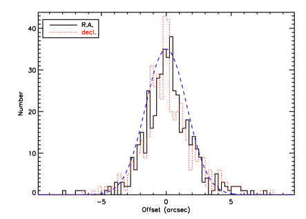
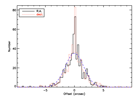
Figure 10 (left panel) shows the pointing offsets estimated using the Gaussian-fitting technique. Of the 581 GBS observations, 115 did not fit our relaxed criteria and no offsets could be measured. Of the remaining 466 observations, the full range of offsets measured in Right Ascension and declination ran between -7 $\farcs$ 8 and 8 $\farcs$ 2 (with similar minima and maxima for each of Right Ascension and declination), with a standard deviation of 1 $\farcs$ 9 and 2 $\farcs$ 0 in Right Ascension and declination, respectively. The distribution of offsets is centred on 0, with mean offsets of $<$ 0 $\farcs$ 2 in both Right Ascension and declination. A notable fraction of the observations showed significant offsets: 214 (46%) had total offsets $\geq 2$ ″, 111 (24%) had total offsets $\geq 3$ ″, and 33 (7%) had total offsets $\geq 5$ ″.

5.1.2 Method 2: Align2d

The second method that we tested involved using Starlink’s align2d command (part of the KAPPA package; Currie & Berry, 2014), which compares all pixels with significant emission in both the observation and reference mosaic to determine an optimal offset. We assumed that the two maps differed only by a simple constant offset, and did not include more-complex terms such as rotation or shear (as was also assumed for the previous method). We first slightly smoothed the observation (by two pixels using KAPPA’s gausmooth command), as we found this improved the reliability of the offsets measured compared to offsets measured using unsmoothed observations. We also tested a range of thresholds for pixels to use in the align2d calculation, and found that the recommended setting of corlimit=0.7¹³¹³13The corlimit parameter can be varied between 0 and 1, with larger values causing more pixels to be excluded from the calculation. worked best. Limiting the calculation to fewer, more reliable pixels resulted in align2d failing to measure an offset in more cases, while those that were measured tended to be consistent between corlimit values, with typical variations of less than 1 pixel (3″).

The right-hand panel of Figure 10 shows the offsets measured by align2d for all of our GBS fields. Of the 581 GBS observations, align2d was unable to measure offsets in only 29 of them, compared with 115 observations without measureable offsets using the Gaussian-fit method. None of the 29 observations had good Gaussian fits (i.e., fits where the offset is larger than the estimated uncertainty), and 22 of the 29 observations had no Gaussian fit, due to insufficient emission features in their respective maps. In a few cases, however, brighter emission was present, but did not yield a single consistent offset value. In these cases, multiple (usually two) peaks were identified by the Gaussian-fit method, but the offsets derived from each peak were mutually inconsistent. The sparse nature of the emission structures in these exceptional cases prevents any conclusion to be made on the cause of the inconsistency in offsets.

For the few observations where our implementation of align2d failed to calculate an offset, we attempted to calculate offset values that would be derived under a variety of different implementations of align2d , using different values of the corlimit parameter, or using an un-smoothed observation. Sometimes, these variations in align2d did yield offset values, however, neither the magnitude nor sign of the derived offsets were consistent between the different methods, again suggesting that simple linear offsets may not be appropriate for these particular observations.

Using the implementation of align2d described above, the full range of pointing offsets runs between -9 $\farcs$ 7 to 7 $\farcs$ 6 (considering Right Ascension and declination separately; both span a similar range). The standard deviation of the pointing offsets is 1 $\farcs$ 7 for Right Ascension and 1 $\farcs$ 8 for declination considered separately. As can be seen from Figure 10 (right panel), despite most observations having small pointing offsets, a non-negligible number of fields have significant pointing errors. We find that 194, or 35%, have total offsets of more than 2″, and 86, or 16%, have total offsets of more than 3″, corresponding to the pixel size for the 450 $\mu$ m and 850 $\mu$ m maps, respectively. Eighteen maps, or about 3.3%, have total offsets in excess of 5″, which is a significant fraction of the 9 $\farcs$ 8 450 $\mu$ m beam.

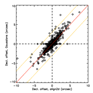
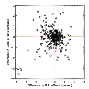
In Figure 11, we show a comparison of all of the offsets measured using both the Gaussian-fit and align2d methods. Clearly, the vast majority of offsets are in good agreement using either method. We carefully visually examined the few observations where align2d and the Gaussian-fit method disagree by more than 3″ (one pixel at 850 $\mu$ m, or about one third of the 450 $\mu$ m beam), and found that the align2d offset typically appeared to be the more correct of the two measures. None of the observations with discrepant derived offsets contained many bright compact sources, where the Gaussian-fit method is expected to perform its best. We therefore adopt the align2d method for DR3.

5.2 Impact on Mosaics

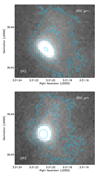
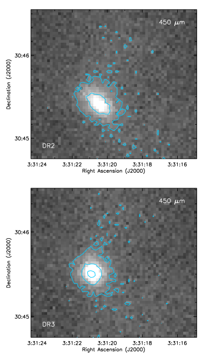
In most fields, many, if not all, of the observations have positions that are corrected by less than 3″, and thus the improvement in the DR3 mosaic over the DR2 mosaic is subtle. There are a handful of fields, however, where the pointing offsets are larger, and the improvement in the final mosaic is more obvious. The one (and only) dramatic example of this is the B1-S field within the PerseusWest mosaic, where pointing offsets for the six observations comprising this field range from -9 $\farcs$ 0 to 3 $\farcs$ 9 in Right Ascension and -9 $\farcs$ 7 to 1 $\farcs$ 0 in declination. Figure 12 shows a comparison of the brightest core in the B1-S field, illustrating the extreme elongation and blurring of the core seen in the DR2 map, even at 850 $\mu$ m. We emphasize that the B1-S field is an extreme outlier in terms of telescope-pointing errors present in the original observations, but it does serve as a good exemplar of how our pointing offset correction is effective. In all other fields, the improvement is subtle at best at 850 $\mu$ m, and is still minor at 450 $\mu$ m. Because these offset corrections are small, it was not necessary to perform an entire additional external-mask reduction with the masked areas shifted to account for the offsets in the individual observations. Even in the B1-S field, not shifting the masks for each individual observation still leaves the majority of the compact source emission (down to below 10% of the local peak) lying within the mask for the reduction.

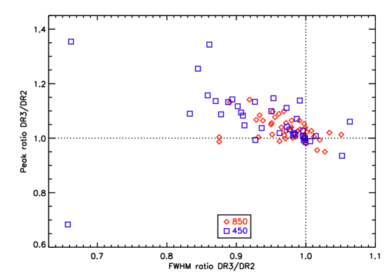
In Figure 13, we show the quantitative improvement of the DR3 maps over the DR2 maps. We ran CUPID’s gaussfit on all of the mosaics created using both DR2 and DR3, and then searched for positional matches between the two catalogues, at each wavelength independently. We restricted our analysis to compact and bright sources to minimize uncertainties in the Gaussian fit parameters. We show only sources which had measured peak fluxes of at least 50 times the local noise level and sizes of FWHM $<25$ ″. In the figure, we see that most of the fitted sources lie in the top left corner, where they would be expected to lie if DR3 tended to reduce the amount of blurring present in the final mosaics. At 850 $\mu$ m, the ratio of FWHM values for DR3 versus DR2 is $0.97\pm 0.04$ and the ratio of peak fluxes is $1.03\pm 0.04$ (mean and standard deviation quoted for both). At 450 $\mu$ m, those same ratios are $0.93\pm 0.09$ and $1.07\pm 0.11$ respectively. As expected, the improvement in DR3 images tends to be larger at 450 $\mu$ m, although there is significant scatter in all relationships. We expect that some of the Gaussian fits may be confused with the presence of diffuse extended structure around the compact-sources fit, and that a careful source-by-source fitting would reduce the scatter in the ratios listed above. Underlining this fact, we note that the 450 $\mu$ m source with a peak-flux ratio less than 0.7 lies in the integral shaped filament within Orion A, in a region known for bright complex emission structures on a variety of scales. Excluding this one source, the FWHM ratio becomes $0.94\pm 0.07$ and the peak-flux ratio becomes $1.08\pm 0.09$ .

6 Conclusions

In this paper, we present the data-reduction methodology employed by the JCMT Gould Belt Survey, through all three major data releases, DR1 through DR3. All of the DR3 data products, including final mosaics using the external mask reductions, the mask files and CO subtracted 850 $\mu$ m maps, are publicly available in conjunction with this paper. [An address for a DOI (permanent webpage) will be made available with the published version of this paper.] In Section 4, we measured the reliability of emission structures recovered in DR1 and DR2. There, we demonstrate that our two-step reduction process allows us to measure true source properties better than prior methods, and that DR2 provides significant improvements over DR1, while both are expected to provide substantially better recovery of extended structures than the JCMT LR1, as already shown in Mairs et al. (2015)¹⁴¹⁴14We note that the JCMT LR1 was designed to identify the locations of emission peaks but not recover the total emission present.

GBS science tends to concentrate on the more-compact emission structures (cores and filaments) where source recovery is best. For the DR2 method, in our idealized tests that assume isolated emission and a source detection method tuned to the known source locations, we recover $>95$ % of artificial structures with peaks at 3 times the rms, for sizes of 30″ and smaller, and 100% of the structures with peaks at 5 times the rms. These recovered structures also have reliable properties measured, with typical peak flux and size measurements both lying within 15% of the true values for sources with peak fluxes at least 3 times the rms, while the total flux measurements lie within 25% of the true values. In all cases, the observed values can be corrected for the deficit in peak flux, total flux, and size measured to a higher degree of accuracy than the listed percentages. Source recovery statistics and the reliability of measured parameters (peak flux and size) for the full series of artificial Gaussian test inputs are provided for reference in Tables 3 and 5. These numbers should be considered as best-case values if measuring and interpreting source-population properties such as the dense-core mass function. Additional effects, such as the presence of non-Gaussian sources, biases from source detection algorithms, and biases due to source crowding have not been considered here, and are all expected to decrease the fraction of sources recovered and the reliability of their properties. We strongly encourage readers to take care in considering these additional effects for any analyses where our recovery and reliability statistics are being applied.

For the final GBS data release (DR3), we estimate the pointing offset present in each observation, by taking advantage of the fact that the survey observed each location on the sky between four and six times. We test two different methods for calculating the offset present between repeated observations of the same field, and find that the KAPPA program align2d tends to produce the most-reliable results. The pointing offsets estimated are typically small. About 16% of the fields have total offsets of at least 3″, which corresponds to one pixel in the 850 $\mu$ m maps and 1.5 pixels in the 450 $\mu$ m maps, while 3.3% have total offsets of at least 5″. Most mosaics show little discernable difference before and after the pointing offset correction, however, the B1-S field in the PerseusWest mosaic in particular is noticeably improved. The full data-reduction procedure is given in Appendix A (for DR1 and DR2), and Section 5 (for DR3) to allow other groups to reproduce our methods. We remind the reader that for DR3, we applied positional shifts to observations reduced under the DR2 methodology, so all of the reduction parameters implemented in makemap are identical to DR2.

Appendix A Data Reduction Parameters

Here, we summarize the full procedure and parameters used to create maps in DR1 and DR2. Settings are supplied to the makemap algorithm through a ‘dimmconfig’ file¹⁵¹⁵15 More information about the SCUBA-2 data reduction procedure can be found at http://starlink.eao.hawaii.edu/devdocs/sc21.htx/sc21.html..

A.1 DR1

The DR1 automask dimmconfig file contains the following settings.

^$STARLINK_DIR/share/smurf/dimmconfig_bright_extended.lis
numiter=-300
flt.filt_edge_largescale=600
maptol=0.001
itermap=1
noi.box_size=-15
flagfast=600
flagslow=200
flt.filt_edge_largescale_last=200
ast.skip=5
flt.zero_snr=5
flt.zero_snrlo=3
noi.box_type=1
flt.ring_box1=0.5
flt.filt_order=4
com.sig_limit=5
ast.zero_snr=5
ast.zero_snrlo=0

The DR1 external-mask dimmconfig file is nearly identical, with only the final two parameters changed to the following assignments.

ast.zero_mask=1
ast.zero_snr=0

In DR1, we created a mosaic of individually reduced observations using their mean, for both the automask and external-mask mosaics. Mask creation in DR1 was not completely identical between regions, as individual region team leads experimented with different schemes. The most commonly adopted scheme was to include in the mask all pixels lying above a signal to noise threshold of 2 in the automask mosaic, and this scheme was the mask-creation method tested in our analysis here.

A.2 DR2

The dimmconfig file for the DR2 automask reduction contained the following lines.

^$STARLINK_DIR/share/smurf/dimmconfig_bright_extended.lis
numiter=-300
flt.filt_edge_largescale=600
maptol=0.001
itermap=1
noi.box_size=-15
flagfast=600
flagslow=200
ast.skip=5
flt.zero_snr=5
flt.zero_snrlo=3
noi.box_type=1
flt.ring_box1=0.5
flt.filt_order=4
com.sig_limit=5
ast.zero_snr=3
ast.zero_snrlo=2
ast.filt_diff=600
ast.zero_lowhits = 0.1
ast.zero_union=0

The dimmconfig file for the DR2 external-mask reduction contained nearly identical lines, with the final five lines above being replaced with the following lines.

ast.zero_mask=1
ast.zero_snr=0

For mosaicking, we combined the observations using a median combination scheme for the automask mosaic, first clipping each observation to the same zone as considered for the automask via the ast.zero_lowhits parameter (i.e., excluding the noisy edge pixels). A mean combination scheme was used for the external-mask mosaic. Masks were created uniformly across regions for DR2. We used all pixels in the automask mosaic lying above a signal-to-noise threshold of 3 which were in zones of 20 or more contiguous pixels (determined using CUPID’s clumpfind).

A.3 Summary of Differences Between DR1 and DR2

Many of the key differences in DR1 and DR2 have already been extensively discussed in Mairs et al. (2015), particularly the change in the parameters ast.zero_snr and ast.zero_snrlo, which effectively allow more pixels to be recognized for having real astronomical signal in the automask reduction in DR2. An important parameter not discussed in Mairs et al. (2015) is the removal of the parameter flt.filt_edge_largescale_last in DR2. When included, this parameter allowed for a stronger filtering of the map outside of the automask or external mask area in the final iteration. Excluding it allowed more real large and faint structures to be present in the final reduced map, with the downside of also increasing large-scale noise features. Switching the mosaicking method to use a median combination for DR2 helped to reduce the presence of these large-scale noise features in the final automask mosaic¹⁶¹⁶16We therefore emphasize that the DR2 automask settings should not be applied for reductions where only a few observations were taken. In this case, large-scale noise features are likely to propagate through to the final automask mosaic and hence also be included in the mask used for the second round of reductions.. Neither the flt.filt_edge_largescale_last parameter nor the median mosaic method had been tested at the time of the publication of Mairs et al. (2015).

A.4 CO Subtraction

The 850 $\mu$ m observing band contains the ¹²CO(3–2) emission line (e.g., Johnstone et al., 2003), which in some instances can contribute significantly to the total emission observed. A full discussion on CO emission and best practices for removing it from the 850 $\mu$ m continuum data is given in Drabek et al. (2012), and an updated version is given in Parsons et al. (2018). Here, we provide a summary of the process used by the GBS for reference.

In short, the procedure involves using the ¹²CO(3–2) integrated intensity map to estimate the contribution to emission observed by SCUBA-2. This emission is subtracted directly from the raw-data time stream so that it will be subject to the same filtering, etc, as the 850 $\mu$ m observations are.

We convert the CO integrated intensity map into the effective continuum emission based on the weather conditions present for each 850 $\mu$ m observation. We multiply by the following factor, $C$ , updated from those originally presented in Drabek et al. (2012) to account for the SCUBA-2 beamsize measurements presented in Dempsey et al. (2013).
$0\leq\tau<0.03,C=2.93e-3\\ 0.03\leq\tau<0.07,C=3.14e-3\\ 0.07\leq\tau<0.10,C=3.24e-3\\ 0.10\leq\tau<0.16,C=3.45e-3\\ 0.16\leq\tau<0.20,C=3.55e-3\\$ where $C$ is in units of (mJy arcsec^-2)(K km s^-1)^-1 and $\tau$ is the optical depth of the atmosphere measured at 250 GHz. Note that these scale factors were recently updated in Parsons et al. (2018), but as the difference is $<<$ 5%, we did not re-run CO subtraction with the updated values.

The scaled CO integrated intensity map is then aligned with the SCUBA-2 external mask, and subtracted using the fakemap parameter in makemap. For DR3 only, we additionally eliminated noisy pixels in the CO integrated intensity map. To do this, we slightly smoothed the CO integrated intensity map (using KAPPA’s gausmooth command with a smoothing scale of 2 pixels), and zeroed out pixels with a signal-to-noise ratio of less than 5. Testing by the data reduction team showed that this procedure is able to reduce the over-subtraction of CO when the HARP CO map has very noisy edges.

Appendix B Difference Maps

B.1 Visual Comparison

As noted in Section 4, by subtracting the original mosaics with no artificial sources added from the reduced maps where the artificial Gaussians had been added into the time stream, we are able to determine the precise contribution of the artificial sources to the final map. This allows us to test the effects of filtering alone, without including the influence of noise.

Figure 14 shows four examples of these difference maps, examining the same artificial Gaussian cases as in the previous Figures 4 and 5. As can be seen from comparing Figure 14 and Figure 4, the compact artificial Gaussians in the reduced images appear similar to their initial models. Wide artificial Gaussians (particularly the bottom-right panel example), however, are substantially fainter after passing through the reduction pipeline.

B.2 Quantitative Measures

In Figure 15, we show the fraction of artificial Gaussians recovered within each of the difference maps. While this measurement is never possible in real observations, it is helpful to examine the circumstances under which artificial Gaussian sources pass through the data-reduction pipeline. Figure 15 shows the fraction of artificial Gaussians that are recovered as a function of Gaussian input peak flux (horizontal axis) and split by Gaussian input size (different colours). Across all reduction methods, it is clear that brighter and more compact Gaussians are the easiest to recover, as expected. The difference between DR1 and DR2 is also stark, where larger and fainter structures are much more likely to be lost following the DR1 procedure. This finding confirms our decision to switch to the DR2 procedure. We note that DR1 includes a harsher filtering level during the final iteration, which is undoubtedly responsible for the major loss of larger-scale structures in the automask reduction compared with DR2. Such filtering would then propagate through to the external-mask reduction through the use of a more compact mask.

A comparison between the automask and external-mask reductions shows at best marginal improvements in the fraction of sources recovered. This trend is understandable, as structures not recovered in the automask reduction will by definition not be included in the mask used for the external-mask reduction. Instead, we expect improvements in the external-mask reduction to come primarily in the form of more accurate recovery of source properties (i.e., peak flux, size, and total flux). Figures 16 and 17 examine this point in more detail.

Figure 16 shows the ratio of the measured peak flux to the initial input peak flux for each artificial Gaussian that was found in the difference maps. As in Figure 15, a comparison between DR1 and DR2 shows that DR2 provides significantly more-accurate peak-flux measurements across the entire grid of artificial Gaussian parameters. A comparison of the external-mask reductions and the automask reductions similarly shows that the external-mask reductions improve peak-flux recovery, particularly for the largest Gaussians. Despite the overall better performance of DR2, however, we note that the largest emission structures ( $\sigma=150$ ″) are still poorly recovered, with measured peak fluxes of less than 15% of their true value for moderately bright sources. Nevertheless, the GBS is mainly focused on dense cores which have typical sizes of $\sigma\sim 10$ ″¹⁷¹⁷17For GBS cloud distances of 100 pc to 500 pc, $\sigma=10$ ″ corresponds to a physical diameter of 0.01 pc to 0.06 pc., which are generally well recovered. For a compact Gaussian with a typical flux cutoff of five times the local noise, we recover peak fluxes to better than 95% of their input value.

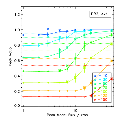Figure 17 similarly shows the Gaussian sizes recovered for each of the reductions, plotting the ratio of the recovered Gaussian size to the input size for all sources that were recovered. As with the previous figures, DR2 shows a clear improvement over DR1 in returning accurate source sizes, while the difference between automask and external-mask reductions is subtler, and is primarily apparent for the largest and brightest artificial sources. As in Figure 16, source properties are poorly recovered for the largest Gaussians, regardless of their peak brightness, but sources with properties similar to dense cores are well recovered.

Finally, Figure 18 similarly shows the ratio of the total flux recovered for each of the reductions compared to its input value. The DR2 reductions again show a clear improvement over DR1, while the external-mask reduction improves the total flux recovered for the largest and faintest sources, although these are still poorly recovered. The total flux is, however, well recovered for compact sources.

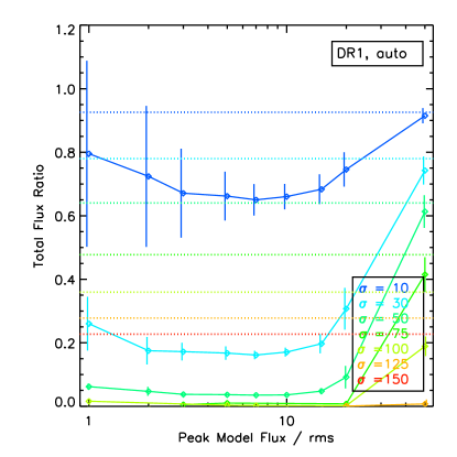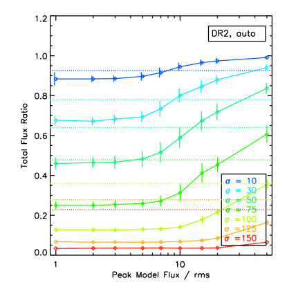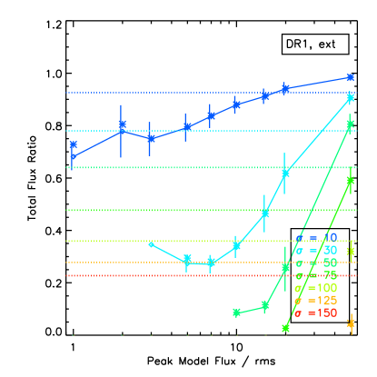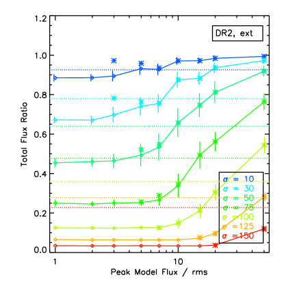Appendix C Large Tables

Here, we include the large tables discussed earlier in the paper. In Table 4, we present a summary of the noise properties of each field observed for the survey.

\startlongtable

Table 4: Approximate Noise Per Observed Area

Region^a^aRegion name, mosaic name, region code, field name, and centre position. The region name corresponds to the name of the molecular cloud, while the mosaic name corresponds to the GBS name given for each mosaic of (usually contiguous) SCUBA-2 observations. There are several mosaics for some molecular clouds. The region (or observing) code and field name are listed in the JCMT archive as Proposal ID and Target Name (http://www.cadc-ccda.hia-iha.nrc-cnrc.gc.ca/en/jcmt/). Observations taken during science verification (SV) were observed under the code MJLSG22. Here, they are combined with observations taken under regular observing, using the standard code for that cloud. An asterisk in the ‘Notes’ column denotes observations that include SV data.	Mosaic^a^aRegion name, mosaic name, region code, field name, and centre position. The region name corresponds to the name of the molecular cloud, while the mosaic name corresponds to the GBS name given for each mosaic of (usually contiguous) SCUBA-2 observations. There are several mosaics for some molecular clouds. The region (or observing) code and field name are listed in the JCMT archive as Proposal ID and Target Name (http://www.cadc-ccda.hia-iha.nrc-cnrc.gc.ca/en/jcmt/). Observations taken during science verification (SV) were observed under the code MJLSG22. Here, they are combined with observations taken under regular observing, using the standard code for that cloud. An asterisk in the ‘Notes’ column denotes observations that include SV data.	Region^a^aRegion name, mosaic name, region code, field name, and centre position. The region name corresponds to the name of the molecular cloud, while the mosaic name corresponds to the GBS name given for each mosaic of (usually contiguous) SCUBA-2 observations. There are several mosaics for some molecular clouds. The region (or observing) code and field name are listed in the JCMT archive as Proposal ID and Target Name (http://www.cadc-ccda.hia-iha.nrc-cnrc.gc.ca/en/jcmt/). Observations taken during science verification (SV) were observed under the code MJLSG22. Here, they are combined with observations taken under regular observing, using the standard code for that cloud. An asterisk in the ‘Notes’ column denotes observations that include SV data.	Field^a^aRegion name, mosaic name, region code, field name, and centre position. The region name corresponds to the name of the molecular cloud, while the mosaic name corresponds to the GBS name given for each mosaic of (usually contiguous) SCUBA-2 observations. There are several mosaics for some molecular clouds. The region (or observing) code and field name are listed in the JCMT archive as Proposal ID and Target Name (http://www.cadc-ccda.hia-iha.nrc-cnrc.gc.ca/en/jcmt/). Observations taken during science verification (SV) were observed under the code MJLSG22. Here, they are combined with observations taken under regular observing, using the standard code for that cloud. An asterisk in the ‘Notes’ column denotes observations that include SV data.	R.A.^a^aRegion name, mosaic name, region code, field name, and centre position. The region name corresponds to the name of the molecular cloud, while the mosaic name corresponds to the GBS name given for each mosaic of (usually contiguous) SCUBA-2 observations. There are several mosaics for some molecular clouds. The region (or observing) code and field name are listed in the JCMT archive as Proposal ID and Target Name (http://www.cadc-ccda.hia-iha.nrc-cnrc.gc.ca/en/jcmt/). Observations taken during science verification (SV) were observed under the code MJLSG22. Here, they are combined with observations taken under regular observing, using the standard code for that cloud. An asterisk in the ‘Notes’ column denotes observations that include SV data.	Decl^a^aRegion name, mosaic name, region code, field name, and centre position. The region name corresponds to the name of the molecular cloud, while the mosaic name corresponds to the GBS name given for each mosaic of (usually contiguous) SCUBA-2 observations. There are several mosaics for some molecular clouds. The region (or observing) code and field name are listed in the JCMT archive as Proposal ID and Target Name (http://www.cadc-ccda.hia-iha.nrc-cnrc.gc.ca/en/jcmt/). Observations taken during science verification (SV) were observed under the code MJLSG22. Here, they are combined with observations taken under regular observing, using the standard code for that cloud. An asterisk in the ‘Notes’ column denotes observations that include SV data.	N_obs^b^bNumber of integrations, and the estimated rms noise for the mosaic of all observations of this field. Note that the number of integrations may include partially completed observations. See the text for details. For an effective beamsize of 14 $\farcs$ 6 and 9 $\farcs$ 8 at 850 $\mu$ m and 450 $\mu$ m respectively (see Dempsey et al., 2013), 1 mJy arcsec^-2 corresponds to 73 mJy beam^-1 and 49 mJy beam^-1, respectively.	rms₈₅₀^b^bNumber of integrations, and the estimated rms noise for the mosaic of all observations of this field. Note that the number of integrations may include partially completed observations. See the text for details. For an effective beamsize of 14 $\farcs$ 6 and 9 $\farcs$ 8 at 850 $\mu$ m and 450 $\mu$ m respectively (see Dempsey et al., 2013), 1 mJy arcsec^-2 corresponds to 73 mJy beam^-1 and 49 mJy beam^-1, respectively.	rms₄₅₀^b^bNumber of integrations, and the estimated rms noise for the mosaic of all observations of this field. Note that the number of integrations may include partially completed observations. See the text for details. For an effective beamsize of 14 $\farcs$ 6 and 9 $\farcs$ 8 at 850 $\mu$ m and 450 $\mu$ m respectively (see Dempsey et al., 2013), 1 mJy arcsec^-2 corresponds to 73 mJy beam^-1 and 49 mJy beam^-1, respectively.	Notes^a^aRegion name, mosaic name, region code, field name, and centre position. The region name corresponds to the name of the molecular cloud, while the mosaic name corresponds to the GBS name given for each mosaic of (usually contiguous) SCUBA-2 observations. There are several mosaics for some molecular clouds. The region (or observing) code and field name are listed in the JCMT archive as Proposal ID and Target Name (http://www.cadc-ccda.hia-iha.nrc-cnrc.gc.ca/en/jcmt/). Observations taken during science verification (SV) were observed under the code MJLSG22. Here, they are combined with observations taken under regular observing, using the standard code for that cloud. An asterisk in the ‘Notes’ column denotes observations that include SV data.
Name	Name	Code		(J2000)	(J2000)		(mJy arcsec^-2)
Perseus	PerseusWest	MJLSG38	L1448-S	03:25:21.4	30:15:46.9	7	0.054	1.63
Perseus	PerseusWest	MJLSG38	L1448-N	03:25:25.1	30:41:57.0	4	0.046	0.61
Perseus	PerseusWest	MJLSG38	L1455-S	03:28:00.2	30:09:26.1	4	0.052	0.88
Perseus	PerseusWest	MJLSG38	NGC1333-S	03:28:40.1	30:53:49.1	6	0.054	1.81
Perseus	PerseusWest	MJLSG38	NGC1333-N	03:29:06.9	31:22:44.7	5	0.049	1.28	*
Perseus	PerseusWest	MJLSG38	L1455-N	03:29:44.6	30:27:12.6	6	0.057	1.79
Perseus	PerseusWest	MJLSG38	B1-S	03:31:32.9	30:46:05.2	6	0.047	1.02
Perseus	PerseusWest	MJLSG38	B1	03:33:12.0	31:07:18.0	8	0.045	0.63	*
Perseus	PerseusWest	MJLSG38	B1-E	03:36:29.2	31:12:58.1	7	0.045	1.35
Perseus	PerseusIC348	MJLSG38	IC348-W	03:39:49.8	31:54:24.4	6	0.047	1.01
Perseus	PerseusIC348	MJLSG38	IC348-C	03:42:10.5	31:51:47.5	6	0.053	1.41
Perseus	PerseusIC348	MJLSG38	IC348-E	03:44:23.6	32:02:03.1	4	0.051	0.78
Perseus	PerseusIC348	MJLSG38	B5	03:47:37.4	32:52:36.5	6	0.047	1.18
Taurus/Auriga	AurigaNorth	MJLSG37	AUR_NW	04:10:08.3	40:07:55.2	6	0.049	1.03
Taurus/Auriga	AurigaNorth	MJLSG37	AUR_CENTRAL-N	04:10:50.3	38:09:23.3	5	0.059	2.33
Taurus/Auriga	TaurusL1495	MJLSG37	L1495-1800-2	04:14:11.1	28:14:11.0	6	0.051	1.53	*,e
Taurus/Auriga	TaurusL1495	MJLSG37	L1495_NW	04:16:40.5	28:37:05.0	2	0.122	5.47	*,f
Taurus/Auriga	TaurusL1495	MJLSG37	L1495_SW	04:16:40.5	28:05:25.0	2	0.127	6.44	*,f
Taurus/Auriga	TaurusL1495	MJLSG37	L1592-1800-1	04:17:54.4	27:47:55.3	6	0.047	1.13
Taurus/Auriga	TaurusL1495	MJLSG37	L1495-1800-1	04:17:54.5	28:18:45.3	6	0.053	1.07	*,e
Taurus/Auriga	TaurusL1495	MJLSG37	L1592-1800-2	04:18:48.9	27:19:32.4	6	0.048	1.11
Taurus/Auriga	TaurusL1495	MJLSG37	L1592-1800-3	04:20:49.1	27:04:07.4	6	0.052	1.55
Taurus/Auriga	AurigaCentral	MJLSG37	AUR_CENTRAL-W	04:20:47.3	37:29:31.8	6	0.049	0.88
Taurus/Auriga	AurigaCentral	MJLSG37	AUR_CENTRAL-E	04:25:10.4	37:10:09.2	6	0.049	0.89
Taurus/Auriga	TaurusSouth	MJLSG37	TAURUSSOUTH5	04:23:21.7	25:03:35.9	6	0.049	1.11
Taurus/Auriga	TaurusSouth	MJLSG37	TAURUSSOUTH4	04:26:57.6	24:35:07.5	6	0.050	0.82
Taurus/Auriga	TaurusSouth	MJLSG37	TAURUSSOUTH3	04:29:38.4	24:34:57.9	6	0.051	1.26
Taurus/Auriga	TaurusSouth	MJLSG37	TAURUSSOUTH2	04:32:20.9	24:23:50.3	6	0.061	1.80
Taurus/Auriga	TaurusSouth	MJLSG37	TAURUSSOUTH1	04:35:17.3	24:07:43.6	6	0.052	1.21
Taurus/Auriga	AurigaLkHa101	MJLSG37	LKHA-101-S	04:30:16.3	35:17:50.9	4	0.051	0.73
Taurus/Auriga	AurigaLkHa101	MJLSG37	LKHA-101-N	04:30:42.5	35:48:12.8	4	0.055	1.09
Taurus/Auriga	TaurusTMC	MJLSG37	TMC1-N	04:38:54.6	26:23:47.8	6	0.047	1.05
Taurus/Auriga	TaurusTMC	MJLSG37	TMC1-SW	04:39:02.0	25:52:10.4	6	0.056	1.68
Taurus/Auriga	TaurusTMC	MJLSG37	TMC1-NE	04:41:00.3	26:09:25.2	7	0.059	2.22
Taurus/Auriga	TaurusTMC	MJLSG37	TMC1-S	04:41:07.7	25:37:47.8	6	0.058	2.14
Orion A	Orion A	MJLSG31	OMC1_TILE17	05:33:09.6	-05:37:52.0	7	0.046	0.88
Orion A	Orion A	MJLSG31	OMC1_TILE1	05:34:20.7	-05:09:53.4	4	0.056	1.02	*
Orion A	Orion A	MJLSG31	OMC1_TILE2	05:34:57.7	-05:40:10.4	4	0.053	0.75
Orion A	Orion A	MJLSG31	OMC1_ISF_CENTRE	05:35:14.2	-05:22:21.5	1	0.179	6.72	*,c
Orion A	Orion A	MJLSG31	OMC1_TILE56	05:35:45.8	-06:07:04.8	4	0.053	1.05
Orion A	Orion A	MJLSG31	OMC1_TILE4	05:35:51.2	-04:46:25.5	5	0.051	0.76
Orion A	Orion A	MJLSG31	OMC1_TILE7	05:36:13.2	-06:31:42.8	6	0.044	0.66
Orion A	Orion A	MJLSG31	OMC1_TILE9	05:38:16.4	-06:39:54.6	7	0.045	1.27
Orion A	Orion A	MJLSG31	OMC1_TILE3	05:36:24.1	-05:17:00.8	4	0.052	0.67
Orion A	Orion A	MJLSG31	OMC1_TILE8	05:36:46.2	-07:02:18.1	6	0.049	1.22
Orion A	Orion A	MJLSG31	OMC1_TILE10	05:38:49.5	-07:10:29.9	6	0.048	1.34	*
Orion A	Orion A	MJLSG31	OMC1_TILE11	05:40:07.2	-07:33:28.8	6	0.043	0.88	*
Orion A	Orion A	MJLSG31	OMC1_TILE16	05:40:58.3	-09:04:00.2	6	0.046	1.07
Orion A	Orion A	MJLSG31	OMC1_TILE12	05:40:58.4	-08:00:40.2	7	0.046	1.18
Orion A	Orion A	MJLSG31	OMC1_TILE14	05:40:58.4	-08:32:20.2	6	0.047	1.13
Orion A	Orion A	MJLSG31	OMC1_TILE13	05:42:49.2	-08:16:30.2	7	0.045	1.11
Orion A	Orion A	MJLSG31	OMC1_TILE15	05:42:49.3	-08:48:10.2	6	0.048	1.01
Orion B	OrionB_N2023	MJLSG41	ORIONBS_450_W	05:40:33.9	-01:48:50.9	4	0.052	0.92
Orion B	OrionB_N2023	MJLSG41	ORIONBS_450_S	05:41:17.3	-02:18:36.3	4	0.051	0.75	g
Orion B	OrionB_N2023	MJLSG41	ORIONBS_850_S	05:41:55.4	-01:24:35.4	7	0.043	1.17
Orion B	OrionB_N2023	MJLSG41	ORIONBS_450_E	05:42:38.8	-01:54:20.8	6	0.049	1.07
Orion B	OrionB_N2023	MJLSG41	ORIONBS_850_N	05:43:39.4	-01:09:35.4	6	0.047	0.99
Orion B	OrionB_N2068	MJLSG41	ORIONBN_450_W	05:45:56.6	00:24:38.9	6	0.055	1.70
Orion B	OrionB_N2068	MJLSG41	ORIONBN_450_S	05:46:18.6	-00:06:32.3	6	0.050	1.14
Orion B	OrionB_N2068	MJLSG41	ORIONBN_850_N	05:47:33.6	00:45:00.1	6	0.047	0.94
Orion B	OrionB_N2068	MJLSG41	ORIONBN_450_E	05:47:55.6	00:13:49.0	6	0.050	1.03
Orion B	OrionB_L1622	MJLSG41	ORIONBN_850_solo	05:54:33.0	01:49:04.7	6	0.053	1.95
Lupus	Lupus	MJLSG34	LUPUSI-SW	15:39:33.7	-34:41:30.0	7	0.063	5.24	d
Lupus	Lupus	MJLSG34	LUPUSI-NW	15:42:45.3	-34:04:30.3	6	0.053	1.70
Lupus	Lupus	MJLSG34	LUPUSI-E	15:45:22.8	-34:21:31.7	6	0.060	2.88
Ophiuchus/Scorpius	OphScoN6	MJLSG32	OPHN-6	16:21:09.5	-20:07:01.4	7	0.045	1.64
Ophiuchus/Scorpius	OphScoMain	MJLSG32	L1688-3	16:25:09.3	-24:23:47.7	5	0.048	1.20
Ophiuchus/Scorpius	OphScoMain	MJLSG32	L1688-1	16:27:03.5	-24:41:57.5	4	0.053	1.10
Ophiuchus/Scorpius	OphScoMain	MJLSG32	L1688-2	16:27:15.7	-24:10:24.7	4	0.058	1.31
Ophiuchus/Scorpius	OphScoMain	MJLSG32	L1688-4	16:29:09.9	-24:28:34.5	4	0.057	1.41
Ophiuchus/Scorpius	OphScoMain	MJLSG32	L1689-2	16:32:04.5	-24:58:26.4	6	0.057	2.57
Ophiuchus/Scorpius	OphScoMain	MJLSG32	L1689-1	16:32:27.4	-24:28:53.7	6	0.047	1.70
Ophiuchus/Scorpius	OphScoMain	MJLSG32	L1709-1	16:32:19.1	-23:56:40.9	7	0.050	1.73
Ophiuchus/Scorpius	OphScoMain	MJLSG32	L1689-3	16:34:34.8	-24:36:39.6	6	0.050	1.87
Ophiuchus/Scorpius	OphScoMain	MJLSG32	L1712-1	16:39:02.2	-24:14:40.8	6	0.053	1.67
Ophiuchus/Scorpius	OphScoN2	MJLSG32	OPHN-2	16:47:40.0	-12:05:00.0	6	0.048	1.49
Ophiuchus/Scorpius	OphScoN3	MJLSG32	OPHN-3	16:50:53.6	-15:21:46.0	6	0.051	1.88
Pipe	PipeB59	MJLSG39	PIPE-B59	17:11:33.4	-27:26:35.2	6	0.045	0.69
Pipe	PipeE1	MJLSG39	PIPE-E1	17:34:06.9	-25:39:27.4	6	0.049	1.34
Serpens/Aquila	SerpensMWC297	MJLSG33	SERPENS-MWC297	18:28:13.8	-03:43:58.3	6	0.053	1.72
Serpens/Aquila	SerpensMain	MJLSG33	SERPENSNH3	18:29:11.2	00:28:37.7	6	0.045	0.74
Serpens/Aquila	SerpensMain	MJLSG33	SERPENSMAIN1	18:29:59.7	01:14:21.9	4	0.060	0.99
Serpens/Aquila	Aquila	MJLSG33	SERPENSS-NW	18:29:30.6	-01:47:30.3	5	0.051	0.79
Serpens/Aquila	Aquila	MJLSG33	SERPENSS-SW	18:30:09.8	-02:17:37.3	5	0.051	0.79
Serpens/Aquila	Aquila	MJLSG33	SERPENSS-NE	18:31:34.6	-01:54:05.3	4	0.053	0.66
Serpens/Aquila	Aquila	MJLSG33	SERPENSS-SE	18:32:13.8	-02:24:12.3	7	0.045	1.16
Serpens/Aquila	SerpensE	MJLSG33	SERPENS-E3	18:36:27.4	-01:17:45.4	6	0.046	1.32
Serpens/Aquila	SerpensE	MJLSG33	SERPENS-E1	18:37:48.8	-01:42:00.9	6	0.050	1.69
Serpens/Aquila	SerpensE	MJLSG33	SERPENS-E2	18:38:32.1	-01:12:15.5	6	0.049	1.82
Serpens/Aquila	SerpensN	MJLSG33	SERPENS-N	18:39:05.5	00:27:26.6	8	0.042	0.70
Corona Australis	CrA	MJLSG35	CRA-1	19:01:35.0	-36:55:56.6	6	0.053	2.04
Corona Australis	CrA	MJLSG35	CRA-2	19:03:34.1	-37:13:58.6	5	0.060	2.37
Corona Australis	CrA	MJLSG35	CRA-E	19:10:23.8	-37:07:53.6	6	0.051	1.16
Cepheus	CepheusSouth	MJLSG40	L1157-W	20:37:24.0	67:57:31.9	6	0.049	2.11
Cepheus	CepheusSouth	MJLSG40	L1157-E	20:44:10.8	67:50:05.9	7	0.052	2.36
Cepheus	CepheusSouth	MJLSG40	L1172-N	21:01:37.3	68:14:21.3	4	0.064	0.98
Cepheus	CepheusSouth	MJLSG40	L1172-S	21:02:33.5	67:44:48.6	6	0.051	2.12
Cepheus	CepheusL1228	MJLSG40	L1228	20:57:42.9	77:38:19.9	6	0.046	0.80
Cepheus	CepheusL1251	MJLSG40	L1251-W	22:29:41.4	75:14:53.0	6	0.049	0.88
Cepheus	CepheusL1251	MJLSG40	L1251-E	22:37:32.7	75:14:53.0	6	0.052	1.82
IC5146	IC5146	MJLSG36	IC5146-W	21:45:35.3	47:37:05.1	6	0.048	1.40
IC5146	IC5146	MJLSG36	IC5146-E	21:48:30.3	47:31:52.5	6	0.045	1.03
IC5146	IC5146	MJLSG36	IC5146-H2	21:53:42.6	47:15:24.2	6	0.050	1.39

^d^dfootnotetext: For historical interest, we note that observations of this field appear to be the final SCUBA-2 data obtained at JCMT before ownership of the telescope was transferred to the East Asian Observatory.

^e^efootnotetext: SV centres offset by

\sim

10 arcmin.

^f^ffootnotetext: Only observed during SV; full survey depth not reached over entire field, however, there is significant overlap with standard survey fields.

^g^gfootnotetext: One of the observations is mis-labeled with code MJLSG31 in the archive.

Table 5 meanwhile provides a summary of the recovered source properties for the two external mask reductions tested.

\startlongtable

Table 5: Properties Recovered for External Mask Reductions

DR	$\sigma$ ^a^aProperties of inserted artificial Gaussians. The Gaussian width, sigma, is given in arcsec, while the peak flux is given in units of the rms noise of the map.	Peak^a^aProperties of inserted artificial Gaussians. The Gaussian width, sigma, is given in arcsec, while the peak flux is given in units of the rms noise of the map.	Peak_rec^b^bTypical recovered properties of artificial Gaussians, as a fraction of their true input value. For the recovered peak flux, width sigma, and total flux, we report both the mean recovered value and the standard deviation. A value of -1 denotes cases where no artificial Gaussians were recovered, as well as cases where only one artificial Gaussian was recovered and the standard deviation is therefore not measureable.		Sigma_rec^b^bTypical recovered properties of artificial Gaussians, as a fraction of their true input value. For the recovered peak flux, width sigma, and total flux, we report both the mean recovered value and the standard deviation. A value of -1 denotes cases where no artificial Gaussians were recovered, as well as cases where only one artificial Gaussian was recovered and the standard deviation is therefore not measureable.		Tot_rec^b^bTypical recovered properties of artificial Gaussians, as a fraction of their true input value. For the recovered peak flux, width sigma, and total flux, we report both the mean recovered value and the standard deviation. A value of -1 denotes cases where no artificial Gaussians were recovered, as well as cases where only one artificial Gaussian was recovered and the standard deviation is therefore not measureable.		Peak_rec,mask^c^cOverlaps with OMC1 Tiles 1 through 4; field name modified from target name in archive of OrionBN-KL for clarity.		Sigma_rec,mask^c^cTypical recovered properties of artificial Gaussians, for the subset of sources that lie within the external mask.		Tot_rec,mask^c^cTypical recovered properties of artificial Gaussians, for the subset of sources that lie within the external mask.
Method	(″)	( $N_{\mathrm{rms}}$ )	Mean	Dev	Mean	Dev	Mean	Dev	Mean	Dev	Mean	Dev	Mean	Dev
DR1	10	1	1.44	0.28	0.76	0.15	0.82	0.29	1.26	0.22	0.83	0.07	0.87	0.31
DR1	10	2	0.92	0.18	0.95	0.20	0.82	0.30	0.99	0.18	0.91	0.17	0.80	0.29
DR1	10	3	0.90	0.15	0.94	0.12	0.78	0.16	0.96	0.14	0.91	0.12	0.78	0.17
DR1	10	5	0.95	0.09	0.94	0.07	0.82	0.11	0.96	0.08	0.93	0.06	0.83	0.10
DR1	10	7	0.97	0.07	0.94	0.04	0.86	0.08	0.97	0.07	0.94	0.04	0.86	0.08
DR1	10	10	0.99	0.04	0.95	0.03	0.90	0.06	0.99	0.04	0.95	0.03	0.90	0.06
DR1	10	15	0.99	0.03	0.96	0.02	0.93	0.05	0.99	0.03	0.96	0.02	0.93	0.05
DR1	10	20	1.00	0.02	0.98	0.02	0.95	0.04	1.00	0.02	0.98	0.02	0.95	0.04
DR1	10	50	1.00	0.01	1.00	0.01	0.99	0.01	1.00	0.01	1.00	0.01	0.99	0.01
DR1	30	1	1.14	-1	0.34	-1	0.13	-1	-1	-1	-1	-1	-1	-1
DR1	30	2	0.64	0.09	0.65	0.05	0.28	0.06	0.71	-1	0.69	-1	0.34	-1
DR1	30	3	0.48	0.07	0.70	0.06	0.23	0.04	0.52	0.04	0.71	0.04	0.26	0.04
DR1	30	5	0.48	0.06	0.71	0.05	0.24	0.04	0.51	0.04	0.70	0.05	0.25	0.04
DR1	30	7	0.54	0.06	0.71	0.03	0.27	0.03	0.56	0.06	0.71	0.03	0.28	0.04
DR1	30	10	0.67	0.07	0.73	0.02	0.36	0.05	0.69	0.06	0.73	0.02	0.37	0.05
DR1	30	15	0.82	0.07	0.76	0.03	0.48	0.07	0.82	0.07	0.76	0.03	0.48	0.07
DR1	30	20	0.92	0.04	0.83	0.04	0.64	0.08	0.92	0.04	0.83	0.04	0.64	0.08
DR1	30	50	1.00	0.01	0.96	0.01	0.93	0.03	1.00	0.01	0.96	0.01	0.93	0.03
DR1	50	1	1.00	-1	0.19	-1	0.04	-1	-1	-1	-1	-1	-1	-1
DR1	50	2	-1	-1	-1	-1	-1	-1	-1	-1	-1	-1	-1	-1
DR1	50	3	-1	-1	-1	-1	-1	-1	-1	-1	-1	-1	-1	-1
DR1	50	5	0.23	0.02	0.51	0.05	0.06	0.01	0.20	-1	0.55	-1	0.06	-1
DR1	50	7	0.19	0.02	0.55	0.03	0.06	0.01	0.19	0.02	0.57	0.03	0.06	0.00
DR1	50	10	0.21	0.03	0.56	0.02	0.06	0.01	0.21	0.02	0.56	0.02	0.07	0.01
DR1	50	15	0.33	0.09	0.56	0.01	0.11	0.03	0.38	0.09	0.56	0.01	0.12	0.03
DR1	50	20	0.65	0.16	0.62	0.04	0.26	0.09	0.66	0.15	0.62	0.04	0.26	0.09
DR1	50	50	0.99	0.02	0.91	0.02	0.83	0.05	0.99	0.02	0.91	0.02	0.83	0.05
DR1	75	1	-1	-1	-1	-1	-1	-1	-1	-1	-1	-1	-1	-1
DR1	75	2	-1	-1	-1	-1	-1	-1	-1	-1	-1	-1	-1	-1
DR1	75	3	-1	-1	-1	-1	-1	-1	-1	-1	-1	-1	-1	-1
DR1	75	5	-1	-1	-1	-1	-1	-1	-1	-1	-1	-1	-1	-1
DR1	75	7	-1	-1	-1	-1	-1	-1	-1	-1	-1	-1	-1	-1
DR1	75	10	-1	-1	-1	-1	-1	-1	-1	-1	-1	-1	-1	-1
DR1	75	15	-1	-1	-1	-1	-1	-1	-1	-1	-1	-1	-1	-1
DR1	75	20	0.09	0.03	0.46	0.02	0.02	0.01	0.09	0.02	0.47	0.04	0.02	0.00
DR1	75	50	0.92	0.04	0.81	0.03	0.60	0.06	0.92	0.04	0.81	0.03	0.60	0.06
DR1	100	1	-1	-1	-1	-1	-1	-1	-1	-1	-1	-1	-1	-1
DR1	100	2	-1	-1	-1	-1	-1	-1	-1	-1	-1	-1	-1	-1
DR1	100	3	-1	-1	-1	-1	-1	-1	-1	-1	-1	-1	-1	-1
DR1	100	5	-1	-1	-1	-1	-1	-1	-1	-1	-1	-1	-1	-1
DR1	100	7	-1	-1	-1	-1	-1	-1	-1	-1	-1	-1	-1	-1
DR1	100	10	-1	-1	-1	-1	-1	-1	-1	-1	-1	-1	-1	-1
DR1	100	15	-1	-1	-1	-1	-1	-1	-1	-1	-1	-1	-1	-1
DR1	100	20	-1	-1	-1	-1	-1	-1	-1	-1	-1	-1	-1	-1
DR1	100	50	0.75	0.04	0.66	0.03	0.32	0.04	0.75	0.04	0.66	0.03	0.32	0.04
DR1	125	1	-1	-1	-1	-1	-1	-1	-1	-1	-1	-1	-1	-1
DR1	125	2	-1	-1	-1	-1	-1	-1	-1	-1	-1	-1	-1	-1
DR1	125	3	-1	-1	-1	-1	-1	-1	-1	-1	-1	-1	-1	-1
DR1	125	5	-1	-1	-1	-1	-1	-1	-1	-1	-1	-1	-1	-1
DR1	125	7	-1	-1	-1	-1	-1	-1	-1	-1	-1	-1	-1	-1
DR1	125	10	-1	-1	-1	-1	-1	-1	-1	-1	-1	-1	-1	-1
DR1	125	15	-1	-1	-1	-1	-1	-1	-1	-1	-1	-1	-1	-1
DR1	125	20	-1	-1	-1	-1	-1	-1	-1	-1	-1	-1	-1	-1
DR1	125	50	0.19	0.15	0.34	0.06	0.03	0.03	0.25	0.14	0.35	0.07	0.04	0.04
DR1	150	1	-1	-1	-1	-1	-1	-1	-1	-1	-1	-1	-1	-1
DR1	150	2	-1	-1	-1	-1	-1	-1	-1	-1	-1	-1	-1	-1
DR1	150	3	-1	-1	-1	-1	-1	-1	-1	-1	-1	-1	-1	-1
DR1	150	5	-1	-1	-1	-1	-1	-1	-1	-1	-1	-1	-1	-1
DR1	150	7	-1	-1	-1	-1	-1	-1	-1	-1	-1	-1	-1	-1
DR1	150	10	-1	-1	-1	-1	-1	-1	-1	-1	-1	-1	-1	-1
DR1	150	15	-1	-1	-1	-1	-1	-1	-1	-1	-1	-1	-1	-1
DR1	150	20	-1	-1	-1	-1	-1	-1	-1	-1	-1	-1	-1	-1
DR1	150	50	-1	-1	-1	-1	-1	-1	-1	-1	-1	-1	-1	-1
DR2	10	1	1.59	0.30	0.96	0.25	1.44	0.65	-1	-1	-1	-1	-1	-1
DR2	10	2	1.02	0.16	1.06	0.21	1.14	0.43	-1	-1	-1	-1	-1	-1
DR2	10	3	0.97	0.12	1.03	0.15	1.04	0.35	1.17	-1	1.12	-1	1.42	-1
DR2	10	5	0.99	0.09	1.00	0.08	0.99	0.16	1.03	0.08	1.00	0.06	1.04	0.12
DR2	10	7	0.98	0.07	0.98	0.05	0.95	0.11	0.99	0.06	0.98	0.05	0.95	0.10
DR2	10	10	1.00	0.04	0.99	0.04	0.99	0.08	1.00	0.04	0.99	0.04	0.99	0.08
DR2	10	15	1.00	0.03	0.99	0.02	0.98	0.05	1.00	0.03	0.99	0.02	0.98	0.05
DR2	10	20	1.00	0.02	1.00	0.02	0.99	0.04	1.00	0.02	1.00	0.02	0.99	0.04
DR2	10	50	1.00	0.01	1.00	0.01	1.00	0.01	1.00	0.01	1.00	0.01	1.00	0.01
DR2	30	1	1.43	0.31	1.21	0.30	2.19	1.14	-1	-1	-1	-1	-1	-1
DR2	30	2	0.97	0.22	1.14	0.16	1.26	0.42	-1	-1	-1	-1	-1	-1
DR2	30	3	0.91	0.13	1.00	0.16	0.93	0.33	1.08	0.10	1.07	0.09	1.22	0.12
DR2	30	5	0.87	0.09	0.95	0.07	0.78	0.16	0.91	0.07	0.95	0.08	0.82	0.19
DR2	30	7	0.89	0.08	0.93	0.04	0.78	0.11	0.89	0.08	0.93	0.04	0.78	0.11
DR2	30	10	0.98	0.05	0.97	0.03	0.92	0.09	0.98	0.05	0.97	0.03	0.92	0.09
DR2	30	15	0.98	0.03	0.96	0.02	0.90	0.07	0.98	0.03	0.96	0.02	0.90	0.07
DR2	30	20	1.00	0.03	0.98	0.02	0.96	0.06	1.00	0.03	0.98	0.02	0.96	0.06
DR2	30	50	1.00	0.01	0.99	0.01	0.98	0.03	1.00	0.01	0.99	0.01	0.98	0.03
DR2	50	1	1.22	0.14	1.03	0.19	1.30	0.57	-1	-1	-1	-1	-1	-1
DR2	50	2	0.87	0.18	0.99	0.23	0.87	0.41	-1	-1	-1	-1	-1	-1
DR2	50	3	0.72	0.17	0.96	0.21	0.68	0.32	-1	-1	-1	-1	-1	-1
DR2	50	5	0.72	0.14	0.91	0.12	0.60	0.18	0.79	0.13	0.93	0.07	0.68	0.14
DR2	50	7	0.77	0.13	0.88	0.07	0.59	0.15	0.79	0.11	0.88	0.06	0.62	0.14
DR2	50	10	0.88	0.08	0.88	0.05	0.69	0.12	0.88	0.08	0.88	0.05	0.69	0.12
DR2	50	15	0.92	0.05	0.91	0.03	0.76	0.09	0.92	0.05	0.91	0.03	0.76	0.09
DR2	50	20	0.95	0.05	0.93	0.03	0.83	0.08	0.95	0.05	0.93	0.03	0.83	0.08
DR2	50	50	0.99	0.02	0.97	0.01	0.93	0.04	0.99	0.02	0.97	0.01	0.93	0.04
DR2	75	1	1.49	0.03	0.83	0.07	0.98	0.17	-1	-1	-1	-1	-1	-1
DR2	75	2	0.74	0.13	0.81	0.08	0.48	0.13	-1	-1	-1	-1	-1	-1
DR2	75	3	0.64	0.09	0.82	0.07	0.44	0.09	-1	-1	-1	-1	-1	-1
DR2	75	5	0.48	0.09	0.78	0.11	0.30	0.10	0.54	-1	0.82	-1	0.36	-1
DR2	75	7	0.49	0.10	0.78	0.07	0.30	0.08	0.59	0.06	0.80	0.05	0.37	0.06
DR2	75	10	0.63	0.12	0.76	0.05	0.36	0.10	0.65	0.11	0.76	0.05	0.38	0.10
DR2	75	15	0.80	0.09	0.81	0.04	0.52	0.09	0.80	0.09	0.81	0.04	0.52	0.09
DR2	75	20	0.83	0.05	0.83	0.02	0.58	0.06	0.83	0.05	0.83	0.02	0.58	0.06
DR2	75	50	0.93	0.03	0.92	0.02	0.78	0.05	0.93	0.03	0.92	0.02	0.78	0.05
DR2	100	1	1.23	-1	0.53	-1	0.33	-1	-1	-1	-1	-1	-1	-1
DR2	100	2	0.68	0.07	0.71	0.11	0.34	0.08	-1	-1	-1	-1	-1	-1
DR2	100	3	0.55	0.08	0.67	0.11	0.25	0.08	-1	-1	-1	-1	-1	-1
DR2	100	5	0.39	0.06	0.71	0.08	0.19	0.04	-1	-1	-1	-1	-1	-1
DR2	100	7	0.35	0.06	0.67	0.05	0.16	0.04	0.47	-1	0.64	-1	0.19	-1
DR2	100	10	0.40	0.09	0.66	0.03	0.17	0.04	0.43	0.03	0.65	0.04	0.19	0.03
DR2	100	15	0.53	0.08	0.67	0.03	0.24	0.05	0.53	0.08	0.67	0.03	0.24	0.05
DR2	100	20	0.65	0.08	0.70	0.02	0.32	0.05	0.65	0.08	0.70	0.02	0.32	0.05
DR2	100	50	0.82	0.03	0.83	0.02	0.57	0.04	0.82	0.03	0.83	0.02	0.57	0.04
DR2	125	1	1.21	0.08	0.51	0.00	0.31	0.02	-1	-1	-1	-1	-1	-1
DR2	125	2	0.62	0.04	0.55	0.04	0.18	0.02	-1	-1	-1	-1	-1	-1
DR2	125	3	0.45	0.06	0.58	0.06	0.14	0.02	-1	-1	-1	-1	-1	-1
DR2	125	5	0.33	0.06	0.54	0.07	0.10	0.03	-1	-1	-1	-1	-1	-1
DR2	125	7	0.27	0.03	0.61	0.07	0.10	0.02	-1	-1	-1	-1	-1	-1
DR2	125	10	0.22	0.03	0.63	0.07	0.09	0.02	-1	-1	-1	-1	-1	-1
DR2	125	15	0.25	0.06	0.58	0.05	0.08	0.02	0.28	0.04	0.58	0.05	0.09	0.02
DR2	125	20	0.31	0.06	0.59	0.03	0.11	0.02	0.31	0.06	0.58	0.03	0.11	0.02
DR2	125	50	0.60	0.03	0.70	0.01	0.29	0.03	0.60	0.03	0.70	0.01	0.29	0.03
DR2	150	1	-1	-1	-1	-1	-1	-1	-1	-1	-1	-1	-1	-1
DR2	150	2	-1	-1	-1	-1	-1	-1	-1	-1	-1	-1	-1	-1
DR2	150	3	0.41	0.04	0.43	0.04	0.07	0.01	-1	-1	-1	-1	-1	-1
DR2	150	5	-1	-1	-1	-1	-1	-1	-1	-1	-1	-1	-1	-1
DR2	150	7	0.22	0.04	0.47	0.04	0.05	0.01	-1	-1	-1	-1	-1	-1
DR2	150	10	0.16	0.01	0.61	0.06	0.06	0.01	-1	-1	-1	-1	-1	-1
DR2	150	15	0.14	0.03	0.51	0.03	0.04	0.01	-1	-1	-1	-1	-1	-1
DR2	150	20	0.14	0.05	0.54	0.05	0.04	0.01	0.17	-1	0.51	-1	0.04	-1
DR2	150	50	0.36	0.03	0.59	0.01	0.12	0.02	0.36	0.03	0.59	0.01	0.12	0.02

The authors wish to recognize and acknowledge the very significant cultural role and reverence that the summit of Maunakea has always had within the indigenous Hawaiian community. We are most fortunate to have the opportunity to conduct observations from this mountain. The JCMT has historically been operated by the Joint Astronomy Centre on behalf of the Science and Technology Facilities Council of the United Kingdom, the National Research Council of Canada, and the Netherlands Organisation for Scientific Research. Additional funds for the construction of SCUBA-2 were provided by the Canada Foundation for Innovation. The identification number for the programme under which the SCUBA-2 data used in this paper is MJLSG*. The authors thank the anonymous referee for their constructive feedback which improved this paper. The authors thank the JCMT staff for their support of the GBS team in data collection and reduction efforts. The Starlink software (Currie et al., 2014) is supported by the East Asian Observatory. These data were reduced using a development version from 2015 December 15, version 01683d2c3d. This research used the services of the Canadian Advanced Network for Astronomy Research (CANFAR), which in turn is supported by CANARIE, Compute Canada, University of Victoria, the National Research Council of Canada, and the Canadian Space Agency. This research used the facilities of the Canadian Astronomy Data Centre operated by the National Research Council of Canada with the support of the Canadian Space Agency. Figures in this paper were creating using the NASA IDL astronomy library (Landsman, 1993) and the Coyote IDL library (http://www.idlcoyote.com/index.html). JCM acknowledges support from the European Research Council under the European Community’s Horizon 2020 framework program (2014-2020) via the ERC Consolidator grant ‘From Cloud to Star Formation (CSF)’ (project number 648505). KP acknowledges support from the Ministry of Science and Technology (Taiwan) (Grant No. 106-2119-M-007 -021 -MY3) and the Science and Technology Facilities Council (Grant No. ST/M000877/1). ADC is supported by the STFC consolidated grant ST/N000706/1. JCMT (SCUBA-2)

References

Berry et al. (2007) Berry, D. S., Reinhold, K., Jenness, T., & Economou, F. 2007, in Astronomical Society of the Pacific Conference Series, Vol. 376, Astronomical Data Analysis Software and Systems XVI, ed. R. A. Shaw, F. Hill, & D. J. Bell, 425
Berry et al. (2013) Berry, D. S., Reinhold, K., Jenness, T., & Economou, F. 2013, CUPID: Clump Identification and Analysis Package, Astrophysics Source Code Library, record ascl: 1311.007
Broekhoven-Fiene et al. (2018) Broekhoven-Fiene, H., Matthews, B. C., Harvey, P., et al. 2018, ApJ, 852, 73
Buckle et al. (2009) Buckle, J. V., Hills, R. E., Smith, H., et al. 2009, MNRAS, 399, 1026
Chapin et al. (2013a) Chapin, E., Gibb, A. G., Jenness, T., et al. 2013a, Starlink User Note, 258
Chapin et al. (2013b) Chapin, E. L., Berry, D. S., Gibb, A. G., et al. 2013b, MNRAS, 430, 2545
Chen et al. (2016) Chen, M. C.-Y., Di Francesco, J., Johnstone, D., et al. 2016, ApJ, 826, 95
Currie & Berry (2013) Currie, M. J., & Berry, D. S. 2013, Starlink User Note, 95
Currie & Berry (2014) —. 2014, KAPPA: Kernel Applications Package, Astrophysics Source Code Library, record ascl: 1403.022
Currie et al. (2014) Currie, M. J., Berry, D. S., Jenness, T., et al. 2014, in Astronomical Society of the Pacific Conference Series, Vol. 485, Astronomical Data Analysis Software and Systems XXIII, ed. N. Manset & P. Forshay, 391
Dempsey et al. (2013) Dempsey, J. T., Friberg, P., Jenness, T., et al. 2013, MNRAS, 430, 2534
Drabek et al. (2012) Drabek, E., Hatchell, J., Friberg, P., et al. 2012, MNRAS, 426, 23
Eden et al. (2017) Eden, D. J., Moore, T. J. T., Plume, R., et al. 2017, MNRAS, 469, 2163
Gibb et al. (2013) Gibb, A. G., Jenness, T., & Economou, F. 2013, Starlink User Note, 265
Haig et al. (2004) Haig, D. J., Ade, P. A. R., Aguirre, J. E., et al. 2004, in Proc. SPIE, Vol. 5498, Z-Spec: a broadband millimeter-wave grating spectrometer: design, construction, and first cryogenic measurements, ed. C. M. Bradford, P. A. R. Ade, J. E. Aguirre, J. J. Bock, M. Dragovan, L. Duband, L. Earle, J. Glenn, H. Matsuhara, B. J. Naylor, H. T. Nguyen, M. Yun, & J. Zmuidzinas, 78–94
Herczeg et al. (2017) Herczeg, G. J., Johnstone, D., Mairs, S., et al. 2017, ApJ, 849, 43
Holland et al. (2013) Holland, W. S., Bintley, D., Chapin, E. L., et al. 2013, MNRAS, 430, 2513
Jenness et al. (2013) Jenness, T., Chapin, E. L., Berry, D. S., et al. 2013, SMURF: SubMillimeter User Reduction Facility, Astrophysics Source Code Library, record ascl: 1310.007
Johnstone et al. (2003) Johnstone, D., Boonman, A. M. S., & van Dishoeck, E. F. 2003, A&A, 412, 157
Johnstone et al. (2017) Johnstone, D., Ciccone, S., Kirk, H., et al. 2017, ApJ, 836, 132
Johnstone et al. (2018) Johnstone, D., Herczeg, G. J., Mairs, S., et al. 2018, ApJ, 854, 31
Kackley et al. (2010) Kackley, R., Scott, D., Chapin, E., & Friberg, P. 2010, in Society of Photo-Optical Instrumentation Engineers (SPIE) Conference Series, Vol. 7740, Society of Photo-Optical Instrumentation Engineers (SPIE) Conference Series, 1
Kainulainen et al. (2009) Kainulainen, J., Lada, C. J., Rathborne, J. M., & Alves, J. F. 2009, A&A, 497, 399
Kauffmann et al. (2010) Kauffmann, J., Pillai, T., Shetty, R., Myers, P. C., & Goodman, A. A. 2010, ApJ, 712, 1137
Kirk et al. (2016) Kirk, H., Di Francesco, J., Johnstone, D., et al. 2016, ApJ, 817, 167
Landsman (1993) Landsman, W. B. 1993, in Astronomical Society of the Pacific Conference Series, Vol. 52, Astronomical Data Analysis Software and Systems II, ed. R. J. Hanisch, R. J. V. Brissenden, & J. Barnes, 246
Lane et al. (2016) Lane, J., Kirk, H., Johnstone, D., et al. 2016, ApJ, 833, 44
Mairs et al. (2015) Mairs, S., Johnstone, D., Kirk, H., et al. 2015, MNRAS, 454, 2557
Mairs et al. (2016) —. 2016, MNRAS, 461, 4022
Mairs et al. (2017a) Mairs, S., Lane, J., Johnstone, D., et al. 2017a, ApJ, 843, 55
Mairs et al. (2017b) Mairs, S., Johnstone, D., Kirk, H., et al. 2017b, ApJ, 849, 107
Markwardt (2009) Markwardt, C. B. 2009, in Astronomical Society of the Pacific Conference Series, Vol. 411, Astronomical Data Analysis Software and Systems XVIII, ed. D. A. Bohlender, D. Durand, & P. Dowler, 251
Men’shchikov (2013) Men’shchikov, A. 2013, A&A, 560, A63
Mowat et al. (2017) Mowat, C., Hatchell, J., Rumble, D., et al. 2017, MNRAS, 467, 812
Parsons et al. (2018) Parsons, H., Dempsey, J. T., Thomas, H. S., et al. 2018, ApJS, 234, 22
Pattle et al. (2015) Pattle, K., Ward-Thompson, D., Kirk, J. M., et al. 2015, MNRAS, 450, 1094
Pattle et al. (2017) —. 2017, MNRAS, 464, 4255
Pineda et al. (2009) Pineda, J. E., Rosolowsky, E. W., & Goodman, A. A. 2009, ApJ, 699, L134
Reid et al. (2010) Reid, M. A., Wadsley, J., Petitclerc, N., & Sills, A. 2010, ApJ, 719, 561
Rosolowsky et al. (2010) Rosolowsky, E., Dunham, M. K., Ginsburg, A., et al. 2010, ApJS, 188, 123
Rosolowsky et al. (2008) Rosolowsky, E. W., Pineda, J. E., Kauffmann, J., & Goodman, A. A. 2008, ApJ, 679, 1338
Rumble et al. (2015) Rumble, D., Hatchell, J., Gutermuth, R. A., et al. 2015, MNRAS, 448, 1551
Rumble et al. (2016) Rumble, D., Hatchell, J., Pattle, K., et al. 2016, MNRAS, 460, 4150
Sadavoy et al. (2013) Sadavoy, S. I., Di Francesco, J., Johnstone, D., et al. 2013, ApJ, 767, 126
Sandell & Knee (2001) Sandell, G., & Knee, L. B. G. 2001, ApJ, 546, L49
Shetty et al. (2010) Shetty, R., Collins, D. C., Kauffmann, J., et al. 2010, ApJ, 712, 1049
Stutzki & Guesten (1990) Stutzki, J., & Guesten, R. 1990, ApJ, 356, 513
Ward et al. (2012) Ward, R. L., Wadsley, J., Sills, A., & Petitclerc, N. 2012, ApJ, 756, 119
Ward-Thompson et al. (2007) Ward-Thompson, D., Di Francesco, J., Hatchell, J., et al. 2007, PASP, 119, 855
Ward-Thompson et al. (2016) Ward-Thompson, D., Pattle, K., Kirk, J. M., et al. 2016, MNRAS, 463, 1008
Yoo et al. (2017) Yoo, H., Lee, J.-E., Mairs, S., et al. 2017, ApJ, 849, 69