Thermal conductivity and local thermodynamic equilibrium of stochastic energy exchange models

Abstract.

In this paper we study macroscopic thermodynamic properties of a stochastic microscopic heat conduction model that is reduced from deterministic problems. Our goal is to numerically check how the “low energy site effect” inherited from the deterministic model would affect the macroscopic thermodynamic properties such as the thermal conductivity and the local thermodynamic equilibrium. After a series of numerical computations, our conclusion is that neither the thermal conductivity nor the existence of local thermodynamic equilibrium is qualitatively changed by this effect.

1. Introduction

In general, nonequilibrium statistical mechanics is not as well-developed as its equilibrium counterpart. Mathematical justifications to many fundamental problems in nonequilibrium statistical physics are not complete yet. The derivation of Fourier’s law from microscopic Hamiltonian dynamics is one of such century-old challenge. It is not clear yet how macroscopic thermodynamic laws including Fourier’s law can be rigorously proved from the motion and interactions of a large number of Newtonian particles [1].

A more precise example is a long and thin tube that contains many kinetic particles. A particle only does free motion and elastic collisions. Now assume two ends of this tube is thermalized in a way that the particle collides with a random particle chosen from a Boltzmann distribution when hitting the left or right boundary. When the temperatures of these two Boltzmann distributions are distinct, the system is driven out from its thermal equilibrium by the boundary effect. Needless to say, this problem is far beyond the reach of today’s dynamical systems technique. In fact, most results about dynamical billiards are for one-particle billiard systems [4], with only a few exceptions [22, 21].

In our earlier paper [12], we attempted to reduce this “particle in a tube” problem to a mathematically tractable stochastic energy exchange model by numerical simulations. The idea is to divide the tube into a large number of localized cells as in [2], such that each particle is trapped in a cells, but collisions between particles in adjacent cells are still allowed through the opening between neighboring cells. See Figure 1 for the detail. Then we use numerical tools to investigate the rule of energy exchanges between cells. We refer Section 2.2 for a detailed description of the energy exchange rule. This gives a stochastic energy exchange model that approximates the time evolution of the energy profile of the billiards model. The stochastic energy exchange model consists of a chain of sites that is connected to two heat baths at its ends. Each site carries some energy, which can be exchanged with neighboring sites at exponentially distributed random times. The rule of energy redistribution at an energy exchange is also random. Many rigorous results can be proved for the resultant stochastic energy exchange model. Among which, our earlier paper [13] rigorously proved that the speed of convergence to the steady state, i.e., the nonequilibrium steady state (NESS), of this model is polynomial. On the other hand, a slightly different stochastic exchange model can be derived by working on the time rescaling limit when particles in adjacent cells barely collide [7, 6, 8]. It is known that the speed of convergence of the second model is exponential [9, 17, 20].

Figure 1. A billiards-like microscopic heat conduction model. Each particle is trapped in its own cell. Collisions through the opening between twe cells are allowed. Red and blue sections of the boundary is thermalized in a why that the particle receives a random kick after colliding with these two sections. The random kick mimics a collision with a particle drawn from a Boltzmann distribution.

The slow speed of convergence of the model in [13] is due to the presence of low energy particle. Because of the localization, the next energy exchange will not happen in a long time period if the kinetic energy of one of the involved particle is low. The slow particle has to move to the “gate” by itself in order to exchange energy with others. As a result, the energy transport is temporarily blocked by this low energy particle. The stochastic energy exchange model inherits this feature from the original deterministic heat conduction model. If a site carries a very low amount of energy, it will wait a long time for the next energy exchange. We call this the low energy site effect. Since the energy transport is occasionally halted by low energy sites, one natural question is that: Would the low energy site effect in a stochastic energy exchange model qualitatively changes the thermal conductivity?

A more fundamental question is about the existence of the local thermodynamic equilibrium (LTE). The existence of LTE means that the marginal distribution of the nonequilibrium steady state with respect to finite local sites converges to a thermal equilibrium when the length of the chain approaches to infinity. Heuristically, this implies the existence of a well-defined local temperature. There are very limited rigorous results about the existence of LTE due to its significant difficulty [10, 19, 16], all of which are for very simple heat conduction models. It is also tempting to check, whether the low energy site effect would make the stochastic energy exchange model fail to achieve LTE.

Different from the thermal equilibrium, NESS usually does not have an explicit form. We are able to prove its existence, uniqueness, ergodicity, and hydrodynamic limits in some situations. But in general a detailed description of NESS is not possible. In fact, this is one reason why any rigorous justification of nonequilibrium statistical physics is challenging. Since mathematical studies to the thermal conductivity and LTE are too difficult, we will have to seek help from numerical simulations.

The main subject of this paper is to answer the two questions raised above numerically. In a stochastic energy exchange model, we choose two different rate functions corresponding to exponential and polynomial ergodicity, respectively. The we use law of large numbers of martingale difference sequences to show that the thermal conductivity is both well defined and computable through Monte Carlo simulations. And the marginal distribution of the NESS is obviously well defined and computable because of the ergodicity. Hence it is not difficult to design a series of numerical simulations to compute the thermal conductivity and the marginal distribution. Our simulations are implemented by the Hashing-Leaping Method (HLM) developed in [15], which is significantly faster than most implementation methods of the stochastic simulation algorithm (SSA). Parallel computing is used to collect enough samples.

Our numerical simulations shows that the low energy site effect will not qualitatively affect the thermal conductance, which is supposed to be proportional to the reciprocal of the length of the chain. This implies the existence of a “normal” thermal conductivity. The thermal conductivity of the model with slow speed of convergence can be increased by changing to 2D. Then the effect of low energy site is significantly reduced. The existence of LTE is a more subtle issue. To check it, one needs to accurately compute the marginal distribution of the NESS. However, the slow convergence speed to NESS caused by the low energy effect imposes many challenges to such computation. After working carefully on the sampling technique and the algorithm, we conclude that LTE is achieved in our model regardless affected by the low energy effect or not.

The paper is organized in the following way. The stochastic energy exchange model, its connection to deterministic dynamical system, and relevant rigorous results are introduced in Section 2. Section 3 is about the law of large number and numerical results of the thermal conductivity. The existence of LTE is investigated in Section 4. Section 5 is the conclusion.

2. Model Description

2.1. Reduction from deterministic dynamics

Consider an 1D chain of billiard tables as described in Figure 1, called the locally confined particle system. One disk-shaped particle is “trapped” in a billiard table such that each particle is allowed to collide with those particles in adjacent billiard tables but can not leave its billiard table. In addition, we assume that the boundary of each billiard table is piecewise $C^{3}$ and strictly convex inward, so that it forms a chaotic dynamical billiards system by itself [3]. This model is intensively studied because this is probably the simplest deterministic dynamical system that models the microscopic heat conduction. The kinetic energy is transported through collisions between particles.

Due to the significant difficulty of studying a chaotic multibody system, a natural question is that whether one can reduce this deterministic dynamical system to a Markov process. More precisely, we look for a stochastic energy exchange process that only keep track of the time evolution of the energy profile. Obviously the process of energy evolution is not Markovian. But since a chaotic billiards system has very good statistical properties, we expect this deterministic energy evolution process to be well approximated by a Markov process, at least under some rescaling limit.

There has been two different studies about the reduction from the billiard system in Figure 1 to a Markov process. One study was conducted by [7, 6], which essentially assumes that the gap between two tables is extremely small. Then we can take a time rescaling limit such that the expected number of particle-particle collisions per unit time is still $1$. The conclusion of this study is that at this time rescaling limit, the probability that two particles with energy $(E_{1},E_{2})$ collides during the next time interval with length $\mathrm{d}t\ll 1$ is approximately $\sqrt{E_{1}+E_{2}}\mathrm{d}t$. Now assume the energy exchange process is Markov. Then the interval between two consecutive energy exchanges should be an exponentially distributed random variable, whose rate is $\sim\sqrt{E_{1}+E_{2}}$. We refer readers to [6] for the precise formula of the energy exchange kernel.

The other point of view, however, focuses on the dynamics at the original time scale. If the billiards table is properly chosen, the time distribution of the next particle-particle collision is very close to an exponential distribution. Instead of taking the time rescaling limit, one can numerically probe the slope of the exponential tail of the first collision time. Additional simulations in [12] demonstrate that the conditional distribution of the time duration between two consecutive collisions have the same exponential tail. Therefore, the energy exchange times of the billiards model can be approximated by a Poisson clock. The rate of this clock, or the slope of the exponential tail, is called the stochastic energy exchange rate. When two adjacent particles have energies $(E_{1},E_{2})$, the numerical simulation in [12] shows that the slope of this exponental tail is $\sim\sqrt{\min\{E_{1},E_{2}\}}$. In other words, the rate of the exponential clock about the energy exchange event should be $\sim\sqrt{\min\{E_{1},E_{2}\}}$. This rate respects the dynamics of the billiards system at its original time scale. It is easy to see that a slow particle needs a long time to move to the “gate area” in order to have a collision, which causes the low energy site effect. Hence the next collision time mainly depends on the lower particle energy in a nearest neighbor pair particles. We refer [12] for further discussions about this clock rate.

It remains to discuss the rule of energy redistribution at a collision. The analysis and numerical simulation in [14] shows that although the explicit formula of an energy redistribution is too complicated to be useful, the amount of exchanged energy has positive density everywhere. Hence it is proper to assume that the energy repartition is done in a “random halves” way as described in equation (2.1). More precisely, we assume that the energies of two colliding particles are pooled together at first. Then a (uniformly distributed) random proportion of the total energy goes to the left, and the rest energy goes to the right. This simplified rule has been used in many early studies [9, 10, 20, 17].

2.2. Stochastic energy exchange process

In summary, the locally confined particle system in Figure 1 can be reduced to the following two stochastic energy processes with two different rate functions. Each process corresponds to one approach of model reduction. Consider a chain of $N$ sites carrying energy $E_{1},\cdots,E_{N}$ respectively. An exponential clock is associated to each pair of sites $(E_{i},E_{i+1})$. The rate of this clock is $R(E_{i},E_{i+1})$. When the clock rings, an energy exchange event occurs immediately. The rule of energy exchange is that

(2.1) $$(E^{\prime}_{i},E^{\prime}_{i+1})=(p(E_{i}+E_{i+1}),(1-p)(E_{i}+E_{i+1}))\,,$$

where $p$ is a uniform random variable on $(0,1)$. We assume the rate function $R(E_{i},E_{i+1})$ has two different choices $R=R_{1}(E_{i},E_{i+1})=\sqrt{E_{i}+E_{i+1}}$ and $R=R_{2}(E_{i},E_{i+1})=\sqrt{E_{i}E_{i+1}/(E_{i}+E_{i+1})}$, corresponding to the dynamics at the time rescaling limit and the original time scale, respectively. Note that here we choose $R_{2}(E_{i},E_{i+1})=\sqrt{E_{i}E_{i+1}/(E_{i}+E_{i+1})}$ because it is a smooth function that mimics the shape of $\sqrt{\min\{E_{i},E_{i+1}\}}$, and it admits an explicit thermal equilibrium.

The rule of energy exchange with the boundary is the same. We assume this chain is connected to two heat baths with temperatures $T_{L}$ and $T_{R}$ respectively. Two more exponential clocks with rates $R(T_{L},E_{1})$ and $R(E_{N},T_{R})$ are associated to two ends of the chain respectively. When the left (resp. right) clock rings, the first (resp. last) site updates energy according to the following rule

(2.2) $$E_{1}^{\prime}=p(E_{1}+\mathcal{E}(T_{L}))\quad(\mbox{resp. }E_{N}^{\prime}=p(E_{N}+\mathcal{E}(T_{R})))\,,$$

where $p$ is a uniform random variable on $(0,1)$, and $\mathcal{E}(\lambda)$ mean an exponential random variable with mean $\lambda$.

The stochastic energy exchange process described above generates a Markov process $\Phi_{t}$ on $\mathbb{R}^{N}_{+}$. Let $\mathbf{E}=(E_{1},\cdots,E_{N})\in\mathbb{R}^{N}_{+}$ be a state of the Markov process and $f(\mathbf{E})$ be a measurable function. To distinguish the two rate functions, we denote the Markov process by $\Phi^{1}_{t}$ if the rate function is $R_{1}$ and by $\Phi^{2}_{t}$ if the rate function is $R_{2}$. The upper index is dropped when it does not lead to a confusion.

The infinitesimal generator $\mathcal{L}_{i}$ of $\Phi^{i}_{t}$ for $i=1,2$ is

(2.3) $$\mathcal{L}_{i}f(\mathbf{E}) =\sum_{n=1}^{N-1}R_{i}(E_{n},E_{n+1})[\int_{0}^{1}f(E_{1},\cdots,p(E_{n}+E_{n+1}),(1-p)(E_{n}+E_{n+1}),$$

$$\cdots,E_{N})\mathrm{d}p-f(\mathbf{E})]$$

$$+R_{i}(T_{L},E_{1})[\int_{0}^{\infty}\int_{0}^{p}f(p(E_{1}+x),E_{2},\cdots,E_{N})\frac{1}{T_{L}}e^{-x/T_{L}}\mathrm{d}x\mathrm{d}p-f(\mathbf{E})]$$

$$+R_{i}(E_{N},T_{R})[\int_{0}^{\infty}\int_{0}^{p}f(E_{1},\cdots,E_{N-1},p(E_{N}+x))\frac{1}{T_{R}}e^{-x/T_{R}}\mathrm{d}x\mathrm{d}p-f(\mathbf{E})]\,.$$

2.3. Rigorous results for the stochastic energy exchange process

Let $V(\mathbf{E})$ be a strictly positive function. For any signed measure $\mu$ on $\mathbb{R}^{N}_{+}$, denote

(2.4) $$\|\mu\|_{V}=\int_{\mathbb{R}^{N}_{+}}V(\mathbf{E})|\mu|(\mathrm{d}\mathbf{E})$$

by the $V$-weighted total variation norm and $\|\mu\|_{TV}$ by the total variation norm. Further, let $L_{V}(\mathbb{R}^{N}_{+})$ be the collection of $V$-integrable probability measures.

We have the following results for $\Phi^{1}_{t}$ (from [17]) and $\Phi^{2}_{t}$ (from [13]).

Theorem 2.1.

$\Phi^{1}_{t}$ admits a unique invariant probability measure that is absolutely continuous with respect to the Lebesgue measure. In addition, there exist constants $c>0$ and $\rho\in(0,1)$ such that

$$\|P^{t}(\mathbf{E},\cdot)-\pi\|_{V}\leq cV(\mathbf{E})\rho^{t}$$

for every $\mathbf{E}\in\mathbb{R}^{N}_{+}$, where $V(\mathbf{E})=1+\sum_{i=1}^{N}E_{i}$.

Theorem 2.2.

Assume further that there exists a constant $K\gg T_{L},T_{R}$ such that $R(E_{i},E_{i+1})=\min\{K,\sqrt{\min\{E_{i},E_{i+1}}\}$. Then $\Phi_{t}$ admits a unique invariant probability measure that is absolutely continuous with respect to the Lebesgue measure. In addition, for any $\gamma>0$, there exists $\eta>0$ such that for any $\mu\in L_{V_{\eta}}(\mathbb{R}^{N}_{+})$,

$$\lim_{t\rightarrow\infty}t^{1-\gamma}\|\mu P^{t}-\pi\|_{TV}=0\,,$$

where

(2.5) $$V_{\eta}=\sum_{i=1}^{N}E_{i}+\sum_{m=1}^{N}\sum_{i=1}^{N-m+1}(\sum_{j=0}^{m-1}E_{i+j})^{a_{m}\eta-1}\,,$$

and $a_{m}=1-(2^{m-1}-1)/(2^{N}-1)$ for $m=1,\cdots,N$.

We remark that a slightly different rate function $R(E_{i},E_{i+1})=\min\{K,\sqrt{\min\{E_{i},E_{i+1}}\}$ is used in Theorem 2.2 for technical reasons in order to make a rigorous proof possible in [13]. It has the same scaling as $R_{2}$ in low energy configurations but makes the proof much simpler (which still contains $35$ pages technical calculation). We expect the speed of convergence to the invariant probability measure of $\Phi^{2}_{t}$ to be the same as described in Theorem 2.2. In other words, the ergodicity of $\Phi^{1}_{t}$ and $\Phi^{2}_{t}$ are qualitatively different. The speed of convergence to the steady state is exponential for $\Phi^{1}_{t}$ but polynomial for $\Phi^{2}_{t}$.

3. Comparison of thermal conductivity

As discussed in the previous section, two rate functions generate two Markov processes $\Phi^{1}_{t}$ and $\Phi^{2}_{t}$ with very different asymptotic properties. $\Phi^{2}_{t}$ has a much slower speed of convergence to its invariant probability measure due to the low energy site effect, which is inherited from the deterministic billiard model. As a result, after an energy exchange event of $\Phi^{2}_{t}$, if a site gets a very low amount of energy, the energy transport will be blocked for a while until this low energy site “recovers” by itself. One natural question is that: how much would the low energy site effect affect macroscopic thermodynamic properties? Would it cause an “abnormal” thermal conductivity that depends on the system size? In this section, we will address this issue numerically.

3.1. Thermal conductivity for 1D model

Let $\pi$ be the invariant probability measure of $\Phi_{t}$. The thermal conductivity of the stochastic energy exchange model is defined as

(3.1) $$\kappa =\frac{1}{T_{R}-T_{L}}\int\left\{(\sum_{i=1}^{N-1}R(E_{i},E_{i+1})\int_{0}^{1}p(E_{i}+E_{i+1})\mathrm{d}p-E_{i})\right.$$

$$+R(T_{L},E_{1})(E_{1}-\int_{0}^{\infty}\int_{0}^{1}p(E_{1}+x)e^{-x/T_{L}}\mathrm{d}p\mathrm{d}x)$$

$$\left.+R(E_{N},T_{R})(\int_{0}^{\infty}\int_{0}^{1}p(E_{N}+x)e^{-x/T_{R}}\mathrm{d}p\mathrm{d}x-E_{N})\right\}\pi(\mathrm{d}\mathbf{E})\,.$$

Equation (3.1) reflects the ratio of the energy flux to the temperature gradient within an infinitesimal amount of time when starting from $\pi$. We claim that $\kappa$ is a computable quantity, i.e., the law of large numbers can be applied to $\kappa$. The thermal conductance, denoted by $\mathbf{q}$, is the ratio of $\kappa$ to the system size, i.e., $\mathbf{q}=\kappa/(N+1)$.

Let $t_{0}<t_{1}<t_{2}<\cdots$ be the time at which an energy exchange occurs. Let $J_{i}$ be the energy flux from right to left associated to the energy exchange event occurring at time $t_{i}$. If the energy exchange event is between site $k$ and site $k+1$, we have $J_{i}=E_{k}(t_{i}^{+})-E_{k}(t_{i})$. If the energy exchange is between site $1$ (resp. site $N$) and the left (resp. right) boundary, we have $J_{i}=E_{1}(t_{i})-E_{1}(t_{i}^{+})$ (resp. $J_{i}=E_{N}(t_{i}^{+})-E_{1}(t_{i})$).

Theorem 3.1.

Assume there exists a constant $K\gg T_{L},T_{R}$ such that $R$ can not exceed $K$. In other words, $R_{1}$ and $R_{2}$ are modified to $\min\{K,\sqrt{E_{i}+E_{i+1}}\}$ and $\min\{K,\sqrt{\frac{E_{i}E_{i+1}}{E_{i}+E_{i+1}}}\}$ respectively. Assume further $\pi(|\mathbf{E}|^{2})<\infty$, then

(3.2) $$\kappa=\lim_{T\rightarrow\infty}\frac{1}{T}\frac{1}{T_{R}-T_{L}}\sum_{t_{i}<T}J_{i}<\infty\quad a.s.$$

We remark that two “assumptions” in Theorem 3.1 are actually provable with extra work. Since the theme of the present paper is about numerical computations, we simply assume these properties to avoid further distractions. A closer look to the proofs in paper [17] and [13] reveals that $\pi(\|\mathbf{E}\|_{1}^{2})$ is finite for both $\Phi^{1}_{t}$ and $\Phi^{2}_{t}$. And the assumption of an upper bound $K$ can be removed by using the estimation of expected energy gain introduced in Proposition 5.1 of [17].

Proof.

Let $0<h\ll 1$ be a time step. Let $\Phi_{n}:=\Phi_{hn}$ be the time-$h$ sample chain of $\Phi_{t}$. Let $Y_{n}$ be the total energy flux during the time period $[nh,(n+1)h)$, i.e.,

(3.3) $$Y_{n}=\frac{1}{h}\frac{1}{T_{R}-T_{L}}\sum_{nh\leq t_{i}<(n+1)h}J_{i}\,.$$

Then we have

(3.4) $$\lim_{T\rightarrow\infty}\frac{1}{T}\frac{1}{T_{R}-T_{L}}\sum_{t_{i}<T}J_{i}=\lim_{m\rightarrow\infty}\frac{1}{m}\sum_{n=1}^{m}Y_{n}\,.$$

Hence it is sufficient to prove the law of large numbers for $Y_{n}$.

Let $Z_{n}=\mathbb{E}_{\Phi_{n}}[Y_{n}]$. It is easy to see that $Z_{n}$ is an observable of $\Phi_{n}$. Now let $\mathcal{F}_{n}$ be the $\sigma$-field generated by $\Phi_{0},\cdots,\Phi_{n}$. Let $Y^{\prime}_{n}=Y_{n}-Z_{n}$. It is easy to see that

$$\mathbb{E}[Y^{\prime}_{n}\,|\,\mathcal{F}_{n}]=0\,.$$

Hence $Y^{\prime}_{n}$ is a martingale difference sequence with respect to $\{\mathcal{F}_{n}\}_{n\geq 0}$. It is well known that if

(3.5) $$\sum_{n=1}^{\infty}\frac{\mathbb{E}[|Y^{\prime}_{n}|^{2}]}{n^{2}}<\infty\,,$$

we have

$$\lim_{m\rightarrow\infty}\frac{1}{m}\sum_{n=1}^{m}Y^{\prime}_{n}=0\,.$$

(This is the law of large numbers for martingales, see for example Theorem 3.3.1 of [5].) In addition, we have

(3.6) $$\mathbb{E}[|Y^{\prime}_{n}|^{2}]\leq\mathbb{E}[|Y_{n}|^{2}]\leq(\frac{1}{h}\frac{1}{T_{R}-T_{L}})^{2}\mathbb{E}[\mathbb{E}_{\Phi_{n}}[\sum_{nh\leq t_{i}<(n+1)h}\|\Phi_{t_{i}}+X_{i}\|^{2}_{1}]]\,,$$

where $X_{i}$ are i.i.d. random variables with law $\max\{\mathcal{E}(T_{L}),\mathcal{E}(T_{R})\}$. This is because $J_{i}$ can not exceed the sum of total energy and the energy coming from the boundary. In addition, assume $t_{i},t_{i+1},\cdots t_{i+m}$ are the first $m+1$ energy exchange times right after $nh$, then the update of the total energy is bounded by $\|\Phi_{t_{i+m}^{+}}\|_{1}\leq\|\Phi_{n}\|_{1}+X_{i}+\cdots+X_{m}$.

Since the clock rate is bounded by $K$ from above, it is easy to see that

(3.7) $$\mathbb{E}_{\Phi_{n}}[\sum_{nh\leq t_{i}<(n+1)h}\|\Phi_{t_{i}}\|^{2}_{1}]\leq\mathbb{E}[\sum_{i=1}^{\mathbf{N}}(\|\Phi_{n}\|_{1}+2X_{i})^{2}]\,,$$

where $\mathbf{N}$ is a Poisson random variable with mean $Kh$. Then some straightforward calculation shows that there exist an $h_{0}>0$, such that for any $h$ we have

(3.8) $$\mathbb{E}[\sum_{i=1}^{\mathbf{N}}(\|\Phi_{n}\|_{1}+2X_{i})^{2}]\leq C_{0}\max\{\|\Phi_{n}\|_{1}^{2},1\}\,,$$

where the constant $C_{0}$ only depends on $h_{0}$.

By the law of large number of Markov process, we have

(3.9) $$\mathbb{E}[(\max\{\|\Phi_{n}\|_{1},1\})^{2}]\rightarrow\pi((\max\{\|E\|_{1},1\})^{2})<\pi(\|E\|_{1}^{2})+1<\infty\,.$$

Then by equations (3.6)-(3.9), we have

(3.10) $$\sum_{n=1}^{\infty}\frac{\mathbb{E}[|Y^{\prime}_{n}|^{2}]}{n^{2}}<\infty\,.$$

Hence the condition in equation (3.5) is satisfied, and the law of large numbers of $Y^{\prime}_{n}$ holds. We have

$$\lim_{m\rightarrow\infty}\sum_{n=1}^{m}Y^{\prime}_{n}=0\,.$$

In addition, by the law of large numbers of Markov process, we have

(3.11) $$\frac{1}{m}\sum_{n=1}^{m}Z_{n}\rightarrow\frac{1}{h}\mathbb{E}_{\pi}[\sum_{t_{i}<h}J_{i}]$$

almost surely. And the right hand side of equation (3.11) is finite because clock rates can not exceed $K<\infty$. Therefore, we have

(3.12) $$\lim_{T\rightarrow\infty}\frac{1}{T}\frac{1}{T_{R}-T_{L}}\sum_{t_{i}<T}J_{i}=\lim_{m\rightarrow\infty}\frac{1}{m}\sum_{n=1}^{m}Y_{n}=\frac{1}{m}\sum_{n=1}^{m}Z_{n}+\lim_{m\rightarrow\infty}\sum_{n=1}^{m}Y^{\prime}_{n}=\frac{1}{h}\mathbb{E}_{\pi}[\sum_{t_{i}<h}J_{i}]<\infty$$

almost surely.

By the invariance of $\pi$, the quantity $\frac{1}{h}\mathbb{E}_{\pi}[\sum_{t_{i}<h}J_{i}]$ is independent of $h$. Since $h$ can be arbitrarily small, by equation (3.12), we have

(3.13) $$\lim_{T\rightarrow\infty}\frac{1}{T}\frac{1}{T_{R}-T_{L}}\sum_{t_{i}<T}J_{i}=\lim_{h\rightarrow 0}\frac{1}{h}\mathbb{E}_{\pi}[\sum_{t_{i}<h}J_{i}]=\kappa\,,$$

where $\kappa$ is the infinitesimal flux defined in equation (3.1). ∎

Then we compute thermal conductivities of $\Phi^{1}_{t}$ and $\Phi^{2}_{t}$ by simulating $\kappa$.

Numerical Simulation 1: Let $T_{L}=1$, $T_{R}=2$. According to Theorem 3.1, we can compute the thermal conductance

$$\mathbf{q}=\lim_{T\rightarrow\infty}\frac{1}{T}\frac{1}{N+1}\frac{1}{T_{R}-T_{L}}\sum_{t_{i}<T}J_{i}$$

over a long trajectory. In our simulation $T$ is chosen to be $2\times 10^{6}$. We compute the thermal conductance $\mathbf{q}$ for $N=6,8,10,\cdots,100$. The simulation results for $\Phi^{1}_{t}$ and $\Phi^{2}_{t}$ are presented in Figure 2.

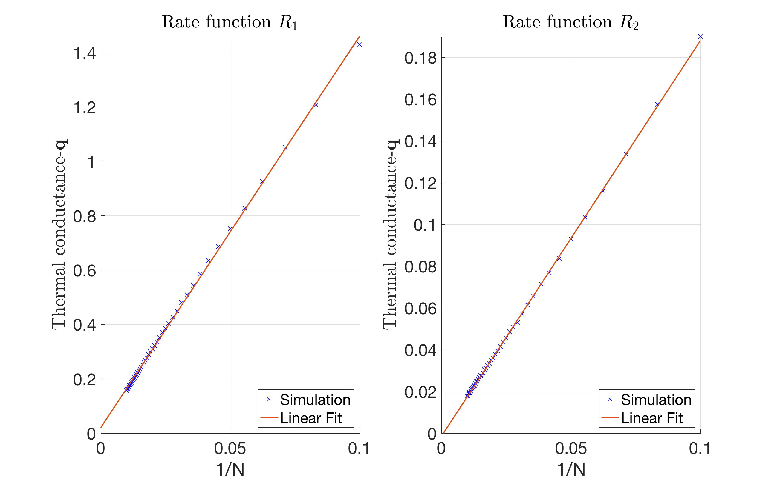
Figure 2. Thermal conductance for $\Phi^{1}_{t}$ and $\Phi^{2}_{t}$. Red line is the linear fit of $\kappa$ versus $1/N$. Left: $R_{1}=\sqrt{E_{1}+E_{2}}$. Right: $R_{2}=\sqrt{E_{1}E_{2}/(E_{1}+E_{2})}$.

According to the plot given above, we see that $\mathbf{q}$ is proportional to $1/N$ for both cases, although the thermal conductance of $\Phi^{2}_{t}$ is much lower. In other words, in spite of a much slower ergodicity and the presence of the low energy site effect, $\Phi^{2}_{t}$ still gives a“normal” thermal conductivity that is independent of the system size. The effect of low energy site will quantitatively reduce the thermal conductivity, but not qualitatively change the scaling of the thermal conductivity. In contrast, note that many harmonic chains and anharmonic chains admit “abnormal” thermal conductivities. We refer the review article [11] for a summary of these results.

3.2. Thermal conductivity of 2D model

The thermal conductivity of a 2D stochastic energy exchange model is also interesting. Obviously the low thermal conductivity of $\Phi^{2}_{t}$ is mainly contributed by the occurence of low energy sites. The occasional occurrence of a low energy site can block the energy transport for a long time, and significantly reduce the thermal conductivity. This problem can be alleviated by increasing the dimension of the system. Instead of an 1D chain, we consider a 2D array of energy sites. The upper and lower edges are adiabatic, while the left and right edges connects to the heat bath.

More precisely, we consider an $M\times N$ array of sites. An exponential clock with rate $R=R_{1}$ or $R_{2}$ is associated to each pair of nearest neighbor sites. When the clock rings, the rule of energy redistribution is same as described in equation (2.1). In addition, sites with indices $(i,1)$ (resp. $(i,N)$) for $i=1,\cdots,M$ are connected to the left (resp. right) heat bath. The rule of energy exchange with heat bath is same as in equation (2.2).

The thermal conductivity $\kappa$ can then be defined and computed analogously. We have

(3.14) $$\kappa =\frac{1}{M}\frac{1}{T_{R}-T_{L}}\int\left\{(\sum_{i=1}^{M}\sum_{j=1}^{N-1}R(E_{i,j},E_{i,j+1})\int_{0}^{1}p(E_{i,j}+E_{i,j+1})\mathrm{d}p-E_{i,j})\right.$$

$$+\sum_{i=1}^{M}R(T_{L},E_{i,1})(E_{i,1}-\int_{0}^{\infty}\int_{0}^{1}p(E_{i,1}+x)e^{-x/T_{L}}\mathrm{d}p\mathrm{d}x)$$

$$\left.+\sum_{i=1}^{M}R(E_{i,N},T_{R})(\int_{0}^{\infty}\int_{0}^{1}p(E_{i,N}+x)e^{-x/T_{R}}\mathrm{d}p\mathrm{d}x-E_{i,N})\right\}\pi(\mathrm{d}\mathbf{E})\,.$$

And again, we denote $\mathbf{q}=\kappa/(N+1)$ as the thermal conductance.

Similar as in the previous subsection, $\kappa$ is a computable quantity. Let $t_{0}<t_{1}<t_{2}<\cdots$ be the time at which an “horizontal” energy exchange, i.e., energy exchange between $E_{i,j}$ and $E_{i,j\pm 1}$ (or heat bath) occurs. Let $J_{k}$ be the energy flux from right to left associated to the energy exchange event occurring at time $t_{k}$. If the energy exchange event is between site $(i,j)$ and site $(i,j+1)$, we have $J_{k}=E_{i,j}(t_{k}^{+})-E_{i,j}(t_{k})$. If the energy exchange is between site $1$ (resp. site $N$) and the left (resp. right) boundary, we have $J_{k}=E_{i,1}(t_{k})-E_{i,1}(t_{k}^{+})$ (resp. $J_{i}=E_{i,N}(t_{k}^{+})-E_{i,N}(t_{k})$).

A similar approach as in Theorem 3.1 implies

(3.15) $$\kappa=\lim_{T\rightarrow\infty}\frac{1}{M}\frac{1}{T_{R}-T_{L}}\sum_{t_{k}<T}J_{k}\,.$$

Numerical Simulation 2: Let $T_{L}=1$, $T_{R}=2$, $N=50$, and $M=1,2,\cdots,20$. By equation (3.15), we can simulate the thermal conductance $\mathbf{q}$ by computing

$$\lim_{T\rightarrow\infty}\frac{1}{M}\frac{1}{T_{R}-T_{L}}\sum_{t_{k}<T}J_{k}$$

over a long trajectory. In our simulation $T$ is chosen to be $1\times 10^{7}$. Then we compare $\mathbf{q}$ for each $M$ from $1$ to $20$. Simulation results of $\mathbf{q}$ vs. $M$ for $\Phi^{1}_{t}$ and $\Phi^{2}_{t}$ are presented in Figure 3.

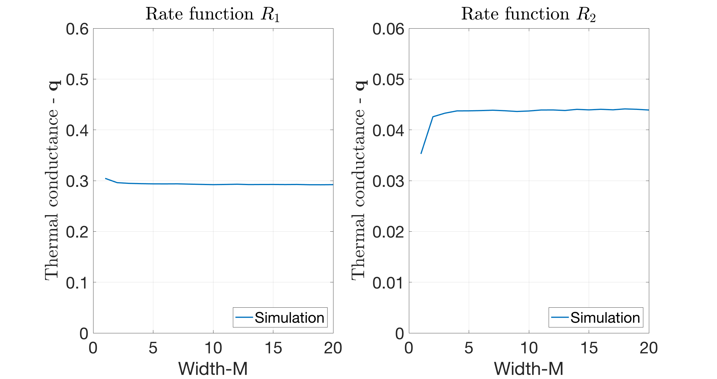
Figure 3. Thermal conductance $\mathbf{q}$ vs. $M$ of the 2D system for $\Phi^{1}_{t}$ and $\Phi^{2}_{t}$. Length of the chain is fixed as $N=50$. $M$ varies from $1$ to $20$. Left: $R_{1}=\sqrt{E_{1}+E_{2}}$. Right: $R_{2}=\sqrt{E_{1}E_{2}/(E_{1}+E_{2})}$.

Figure 3 confirms our speculation. With rate function $R_{1}=\sqrt{E_{1}+E_{2}}$, the thermal conductivity changes inconspicuously even the width of the system increases. With rate function $R_{2}=\sqrt{E_{1}E_{2}/(E_{1}+E_{2})}$, $\mathbf{q}$ (as well as $\kappa$) increases significantly when $M$ changes from $1$ to $2$, and keeps increasing with increasing $M$. This demonstrates the dimension effect. When a site loses most of its energy in an energy exchange and becomes “silent” for a while, the energy transport is completely blocked in an 1D model. With an extra dimension, the energy can still be transported by circumventing the “silent” site. In addition, the probability that the energy transport is completed blocked becomes much lower in a 2D model.

4. Comparison of local thermodynamic equilibrium(LTE)

The local thermodynamical equilibrium (LTE) assumption means that although the entire system is nonequilibrium, the marginal distribution of the steady state with respect to a “local” subset is still close to a thermal equilibrium. The existence of LTE is equivalent to the existence of a well-defined local temperature. In the study of microscopic heat conduction models, the existence of LTE usually means the marginal distribution of NESS with respect to finite many local sites converges to a thermal equilibrium as the length of the chain goes to infinity. We refer [16, 19] for further discussion and known rigorous results about the existence of LTE.

4.1. Nonequilibrium steady state under the LTE assumption

The two rate functions in Section 2 are chosen in a way that the theoretical thermal equilibrium can be explicitly given. We start this subsection with the following Proposition.

Proposition 4.1.

Assume the chain is infinitely long on both sides. The process $\Phi^{1}_{t}$ (resp. $\Phi^{2}_{t}$) admits a family of invariant probability measures

(4.1) $$\pi=\prod_{i=-\infty}^{\infty}\pi_{i}^{T}\quad T>0\,,$$

where $\pi_{i}^{T}$ are i.i.d. exponential random variables (resp. Gamma random variables) with mean $T$ (resp. parameters $1/2$ and $T$).

Proof.

Since there is no energy exchange with the boundary, it is sufficient to check the interaction between $E_{i}$ and $E_{i+1}$.

When starting from the probability distribution $\pi$ given in the theorem, the probability that $\Phi^{1}_{t}$ leaves $(E_{i},E_{i+1})$ on the next infinitesimal time interval $(0,\mathrm{d}t)$ is

$$\sqrt{E_{i}+E_{i+1}}e^{-E_{i}/T}e^{-E_{i+1}/T}\mathrm{d}t\,.$$

On the other hand, when starting from $\pi$, the probability density that $\Phi^{1}_{t}$ enters an infinitesimal neighborhood of $(E_{i},E_{i+1})$ on the same time interval is

(4.2) $$\mathrm{d}t\cdot\int_{0}^{E_{i}+E_{i+1}}\frac{1}{E_{i}+E_{i+1}}\sqrt{x+(E_{i}+E_{i+1}-x)}e^{-x/T}e^{-(E_{i}+E_{i+1}-x)/T}\mathrm{d}x$$

$$= \sqrt{E_{i}+E_{i+1}}e^{-E_{i}/T}e^{-E_{i+1}/T}\mathrm{d}t\,.$$

Therefore, $\pi$ is invariant for $\Phi^{1}_{t}$ if $\pi_{i}$ are i.i.d. exponential distributions.

The case of $\Phi^{2}_{t}$ is the same. The probability that $\Phi^{2}_{t}$ leaves $(E_{i},E_{i+1})$ is

(4.3) $$\sqrt{\frac{E_{i}E_{i+1}}{E_{i}+E_{i+1}}}\cdot\frac{1}{\sqrt{T}\Gamma(1/2)}\frac{1}{\sqrt{E_{i}}}e^{-E_{i}/T}\cdot\frac{1}{\sqrt{T}\Gamma(1/2)}\frac{1}{\sqrt{E_{i+1}}}e^{-E_{i+1}/T}\mathrm{d}t$$

$$= \frac{1}{T\pi}\frac{1}{\sqrt{E_{i}+E_{i+1}}}e^{-(E_{i}+E_{i+1})/T}\mathrm{d}t\,.$$

The probability density that $\Phi^{2}_{t}$ enters an infinitesimal neighborhood of $(E_{i},E_{i+1})$ is

(4.4) $$\mathrm{d}t\cdot\int_{0}^{E_{i}+E_{i+1}}\frac{1}{E_{i}+E_{i+1}}\sqrt{\frac{x(E_{i}+E_{i+1}-x)}{x+(E_{i}+E_{i+1}-x)}}\cdot\frac{1}{\sqrt{T}\Gamma(1/2)}\frac{1}{\sqrt{x}}e^{-x/T}$$

$$\cdot\frac{1}{\sqrt{T}\Gamma(1/2)}\frac{1}{\sqrt{E_{i}+E_{i+1}-x}}e^{-(E_{i}+E_{i+1}-x)/T}\mathrm{d}x$$

$$= \frac{1}{T\pi}\frac{1}{\sqrt{E_{i}+E_{i+1}}}e^{-(E_{i}+E_{i+1})/T}\mathrm{d}t\,.$$

Therefore, $\pi$ is invariant for $\Phi^{2}_{t}$ if $\pi_{i}$ are i.i.d. Gamma distributions. This completes the proof. ∎

This theoretical thermal equilibrium does not work well for a finite chain due to boundary effects. However, we are curious about whether the marginal distribution of the NESS with respect to finite local sites converges to i.i.d. exponential (or Gamma) distributions when $N\rightarrow\infty$. If the answer is yes, then the LTE is established. Note that here we adopt a strict definition of the LTE. We see that LTE is achieved only if the marginal distribution of the NESS with respect to many local sites converges to the thermal equilibrium described before. There are also literatures about weaker versions of LTE [18], i.e., the marginal distribution with respect to one site or one point.

We plan to use the energy profile and the thermal conductivity to preliminarily check whether LTE is achieved. It is not difficult to calculate the theoretical energy flux $J_{i,i+1}$ if we know the joint distribution of $(E_{i},E_{i+1})$. This theoretical flux can be then used to compute a theoretical energy profile. Then we can compare the theoretical energy profile and its empirical counterpart (which is relatively easy to compute).

The following two propositions follow from simple calculations.

Proposition 4.2.

If the joint marginal distribution of the invariant probability measure of $\Phi^{1}_{t}$ with respect to site $E_{i}$ and $E_{i+1}$ is the product measure of two exponential distributions with mean $T$ and $\hat{T}$ respectively, then the mean energy flux from site $i+1$ to site $i$ is

(4.5) $$J_{i,i+1}=\frac{\sqrt{\pi}(3T^{2}+9T^{3/2}\hat{T}^{1/2}+11T\hat{T}+9T^{1/2}\hat{T}^{3/2}+3\hat{T}^{2})}{8(T^{1/2}+\hat{T}^{1/2})^{3}}(\hat{T}-T)\,.$$

Proof.

We have

(4.6) $$J_{i,i+1}=\int_{0}^{\infty}\int_{0}^{\infty}\frac{y-x}{2}\cdot\sqrt{x+y}\cdot\frac{1}{T}e^{-x/T}\cdot\frac{1}{\hat{T}}e^{-y/\hat{T}}\mathrm{d}x\mathrm{d}y\,.$$

Let $u=y-x$ and $v=x+y$. The rest are straightforward calculation about the integral. ∎

Proposition 4.3.

If the joint marginal distribution of the invariant probability measure of $\Phi^{2}_{t}$ with respect to site $E_{i}$ and $E_{i+1}$ is the product measure of two Gamma distributions with parameters $(1/2,T)$ and $(1/2,\hat{T})$ respectively, then the mean energy flux from site $i+1$ to site $i$ is

(4.7) $$J_{i,i+1}=\frac{T^{1/2}\hat{T}^{1/2}(T+3T^{1/2}\hat{T}^{1/2}+\hat{T})}{4\sqrt{\pi}(T^{1/2}+\hat{T}^{1/2})^{3}}(\hat{T}-T)\,.$$

Proof.

We have

(4.8) $$J_{i,i+1}=\int_{0}^{\infty}\int_{0}^{\infty}\frac{y-x}{2}\cdot\sqrt{\frac{xy}{x+y}}\cdot\frac{1}{\sqrt{T}\Gamma(1/2)}e^{-x/T}\cdot\frac{1}{\sqrt{\hat{T}}\Gamma(1/2)}e^{-y/\hat{T}}\mathrm{d}x\mathrm{d}y\,.$$

Let $u=y-x$ and $v=x+y$. The rest are straightforward calculation about the integral. ∎

4.2. Numerical study of the LTE assumption

We propose the following three numerical simulations to check the validity of the LTE assumption. Note that the rule of boundary interaction is different from that in the middle of the chain. Hence marginal distributions with respect to boundary sites always have boundary effects, and the system does not reach thermal equilibrium even if $T_{L}=T_{R}$. We will show that when the length of the chain increases, the boundary effect gradually disappears. At the limit, the marginal distribution with respect to finite many sites that are in the middle of the chain converges to the theoretical thermal equilibrium given by Proposition 4.1.

Numerical Simulation 3. We first simulate the marginal distribution with respect to a single site. Let $T_{L}=1$, $T_{R}=2$, $N=10,20,40,60,80$. We simulate processes $\Phi^{1}_{t}$ and $\Phi^{2}_{t}$ over a long trajectory and collect the energy profile at sampling times $h,2h,\cdots,8\times 10^{6}h$. $h$ is chosen to be $2$ for $\Phi^{1}_{t}$ and $10$ for $\Phi^{2}_{t}$. The time-$h$ skeleton of a time-continuous Markov process preserves its invariant probability measure. Hence we can compute the marginal distribution of the invariant probability measure with respect to each site.

Then we compare the sample with respect to each site with a desired Gamma distribution. This step is done by using the gamfit function in MATLAB. Parameters $(\alpha,\beta)$ of the Gamma distribution with respect to each set are demonstrated in Figure 4 and Figure 5. We can find that the marginal distribution with respect to a non-boundary site is approximately a Gamma distribution with parameters $(1,\beta_{i})$ for $\Phi^{1}_{t}$ and $(1/2,\beta_{i})$ for $\Phi^{2}_{t}$, where $\beta_{i}$ changes with the site index. Note that an exponential distribution with mean $\lambda$ is a Gamma distribution with parameters $(1,\lambda^{-1})$. Hence our numerical result is consistent with the marginal distribution obtained in Proposition 4.1.

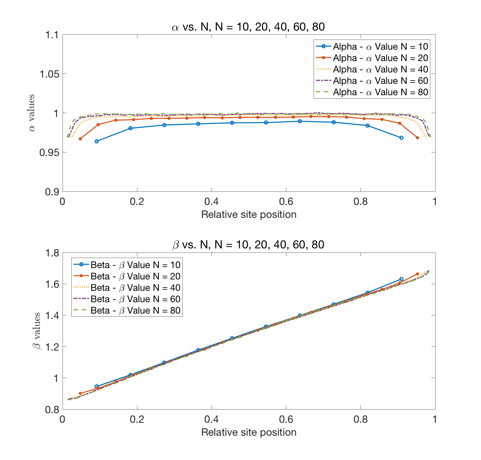
Figure 4. Parameters $\alpha$ and $\beta$ of the Gamma distribution fitted from marginal distributions with respect to all sites. The length of the chain is $N=10,20,40,60,80$. Rate function $R_{1}=\sqrt{E_{1}+E_{2}}$.

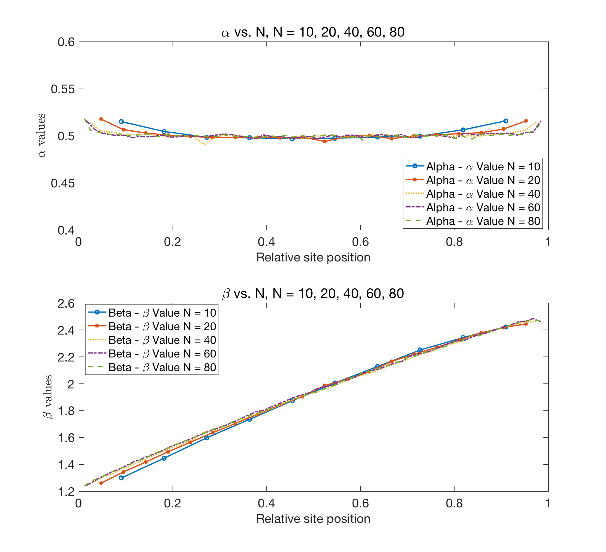
Figure 5. Parameters $\alpha$ and $\beta$ of the Gamma distribution fitted from marginal distributions with respect to all sites. The length of the chain is $N=10,20,40,60,80$. Rate function $R_{2}=\sqrt{E_{1}E_{2}/(E_{1}+E_{2})}$.

The goodness of the fit is done by a Chi-square test. We divide the domain into $31$ bins $[0,0.2),\cdots,[5.8,6.0),[6.0,\infty)$. Let $p_{i}$ be the theoretical probability of the desired Gamma distribution at each interval and $n_{i}$ be the number of samples falling to this interval. We calculate

(4.9) $$\chi^{2}=\sum_{i=1}^{31}\frac{(n_{i}-\mathbf{N}p_{i})^{2}}{\mathbf{N}p_{i}}$$

for each site. If the marginal distribution satisfies a Gamma distribution, the $\chi^{2}$ test statistics should be smaller than the $95$th percentile of a $\chi^{2}$ distribution with $30$ degrees of freedom. Figure 6 and Figure 7 shows our result for the goodness of the fit. We can see that when the chain is long enough, the marginal distribution with respect to a non-boundary site is very closed to a Gamma distribution in both cases, which is exactly the thermal equilibrium we found in Proposition 4.1. In other words, LTE is achieved for a single site in the chain as the length of the chain grows.

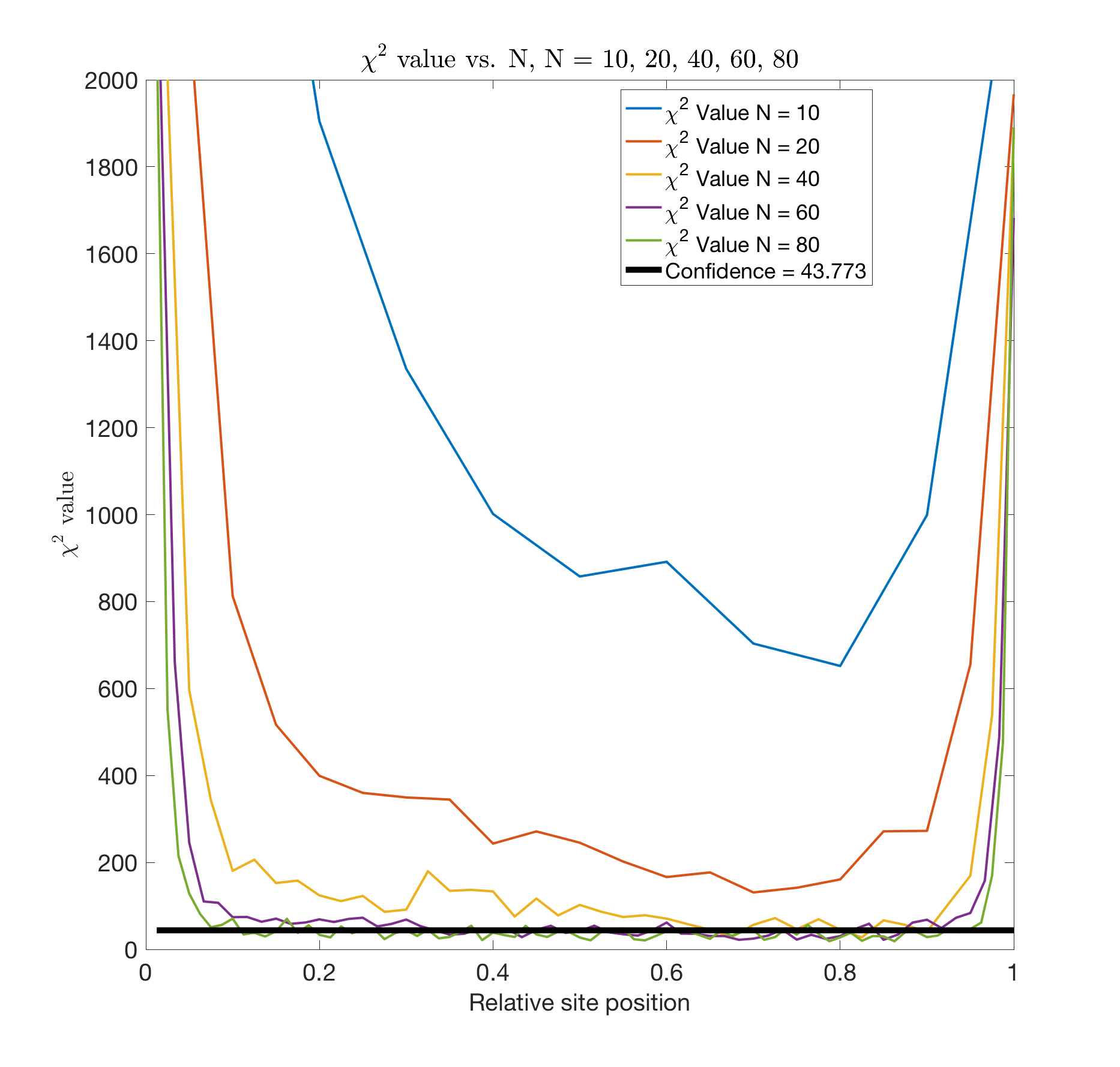
Figure 6. Values of $\chi^{2}$-test statistics (equation (4.9)) of the marginal distribution of each site. $x$-axis: site index. $y$-axis: $\chi^{2}$. Rate function $R_{1}=\sqrt{E_{1}+E_{2}}$.

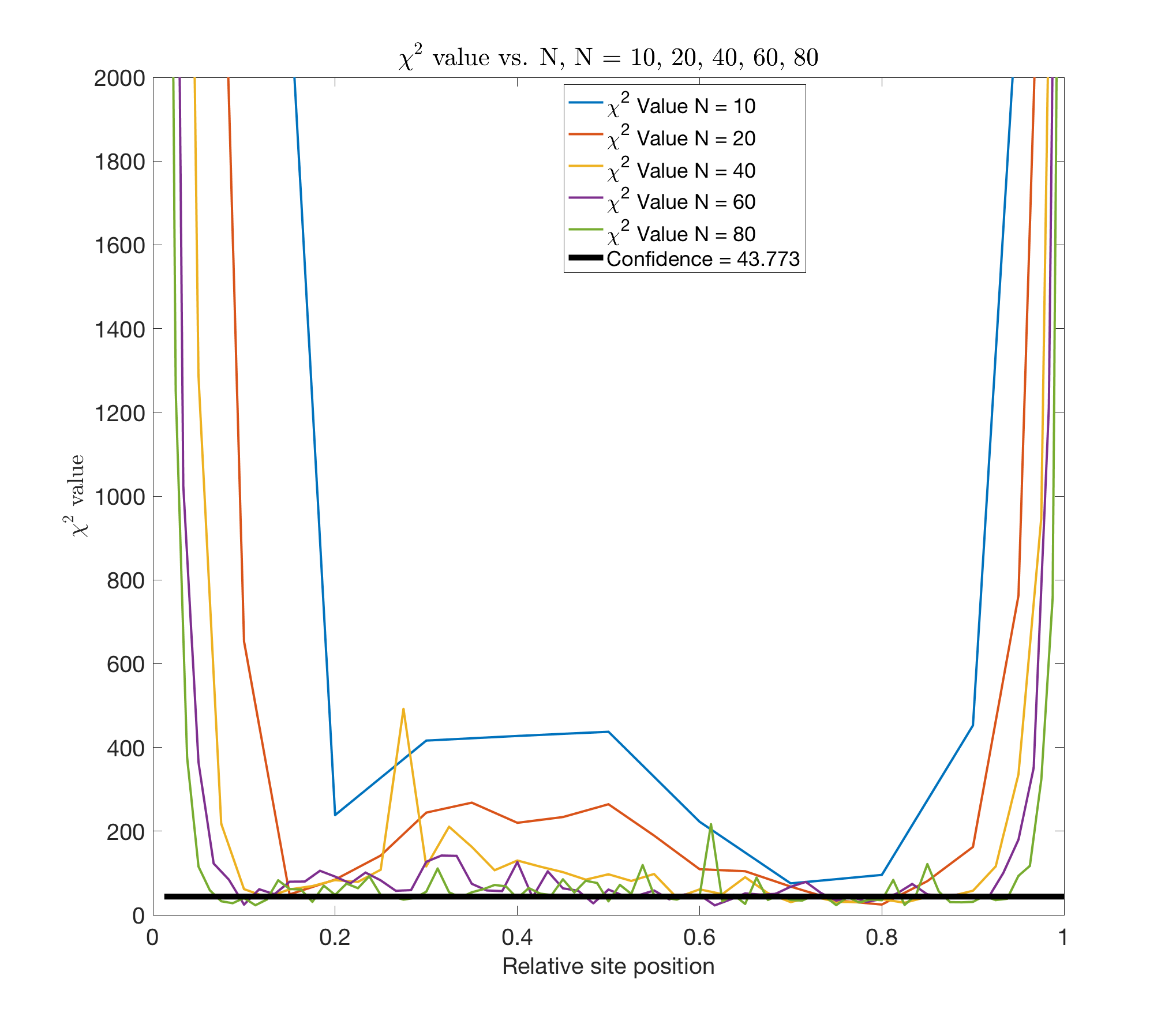
Figure 7. Values of $\chi^{2}$ test statistics (equation (4.9)) of the marginal distribution of each site. $x$-axis: site index. $y$-axis: $\chi^{2}$. Rate function $R_{2}=\sqrt{E_{1}E_{2}/(E_{1}+E_{2})}$.

Numerical Simulation 4. The next task is to use the energy profile to check the LTE assumption. Assume LTE is achieved, the theoretical energy flux can be obtained from equations (4.5) and (4.7). Then we can compare the empirical energy profile with the predicted ones when assuming the LTE. The result of Numerical Simulation 3 shows that at the boundary the marginal distribution is far from the Gamma distribution. Hence we can only use Propositions 4.2 and 4.3 to predict the energy profile in the middle. The predicted energy profile under the LTE assumption is obtained in the following way. Assume that $E_{5}$ and $E_{36}$ are equal to those in the empirical energy profile. Since the mean energy flux $J_{i,i+1}$ is independent of the choice of $i$, we can solve a nonlinear equation involving $E_{6},E_{7},\cdots,E_{35}$ numerically such that $J_{6,7}=J_{7,8}=\cdots=J_{34,35}$, where terms $J_{i,i+1}$ are from equation (4.5) for $\Phi^{1}_{t}$ and (4.7) for $\Phi^{2}_{t}$. This gives the predicted energy profile from site $6$ to site $35$. The predicted and empirical energy profiles for $\Phi^{1}_{t}$ and $\Phi^{2}_{t}$ are compared in Figure 8. We can find that in both cases the predicted energy profile is very close to the empirical one. Note that in the energy profile, the mean energy of the left (resp. right) boundary site is not close to $T_{L}$ (resp. $T_{R}$). This is because the rule of boundary interaction is different from that of non-boundary sites. In particular, the rate of an energy exchange with the left (resp. right) boundary is $R(T_{L},E_{1})$ (resp. $R(E_{N},T_{R})$) regardless the amount of energy drawn at the boundary. Hence the effective temperature “felt” by a boundary site is not the heat bath temperature.

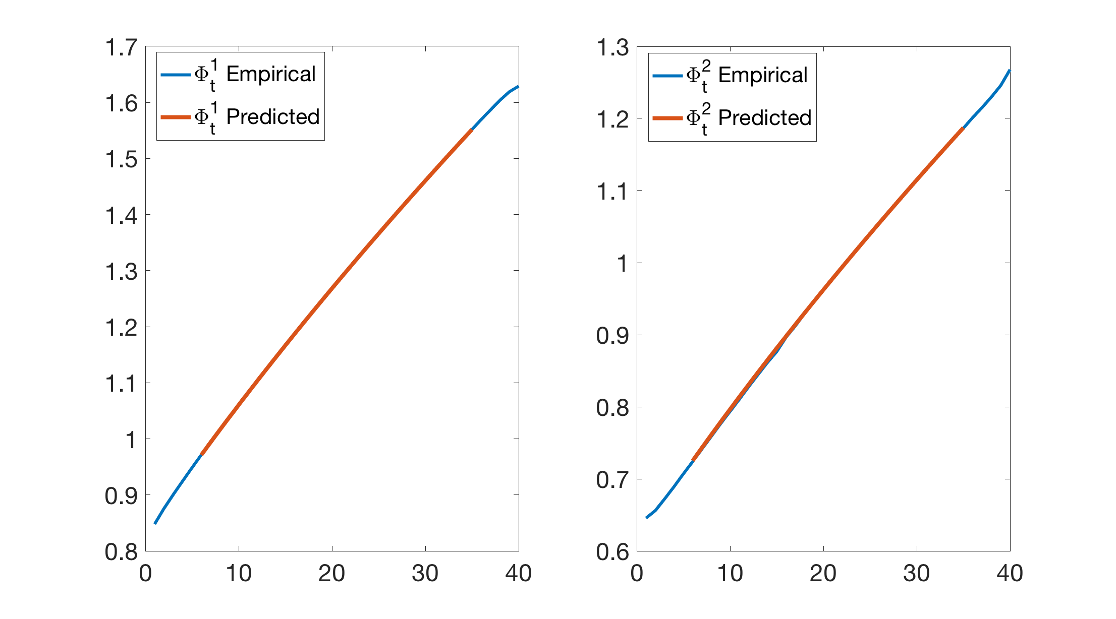
Figure 8. A comparison of predicted and empirical energy profiles. Left panel: $R_{1}=\sqrt{E_{1}+E_{2}}$. Right panel: $R_{2}=\sqrt{E_{1}E_{2}/(E_{1}+E_{2})}$.

The result in Figure 8 suggests that equations (4.5) and (4.7) can produce good approximations of the macroscopic energy profile. However, the energy profile alone is not sufficient for us to claim the existence of LTE, as dependent marginal distributions can still produce the same energy profile. In fact, when the chain is not long enough, the theoretical mean energy flux by assuming LTE is quite different from the empirical energy flux. In order to check whether LTE is achieved, we need to accurately compute the marginal distribution with respect to nearest neighbor sites.

Numerical Simulation 5. Finally, we simulate the joint marginal distribution with respect to two nearest neighbor sites at the center of the chain. We simulate $8$ long trajectories to generate the joint marginal distribution with respect to $(E_{N/2},E_{N/2+1})$ for increasing $N$. For each trajectory, we collect samples of $(E_{N/2},E_{N/2+1})$ at each sampling time $h,2h,\cdots,2\times 10^{8}h$. We choose $h=0.25$ for $\Phi^{1}_{t}$ and $h=1$ for $\Phi^{2}_{t}$ because the average clock rate of $\Phi^{2}_{t}$ is lower. The reason of doing this is because the time-$h$ skeleton of a time-continuous Markov process preserves its invariant probability measure. This approach gives us $1.6\times 10^{9}$ samples. We need these many samples to achieve the accuracy needed for verifying the existence of LTE.

Let $a_{0},a_{1},\cdots,a_{16}=0,0.1,\cdots,1.6$ and $a_{17}=\infty$. We define two auxiliary random variables $Z_{1}$ and $Z_{2}$ that represent the discretization of $E_{N/2}$ and $E_{N/2+1}$ with respect to the partition generated by $a_{0},a_{1},\cdots,a_{17}$, respectively. $Z_{1}=i$ (resp. $Z_{2}=i$) if and only if $E_{N/2}\in[a_{i-1},a_{i})$ (resp. $E_{N/2+1}\in[a_{i-1},a_{i})$). In other words $Z_{1},Z_{2}$ takes the value $1$ to $17$. We use the collected $\mathbf{N}=1.6\times 10^{9}$ samples to estimate the probability distributions of $Z_{1},Z_{2}$ as well as their joint distributions. If $Z_{1},Z_{2}$ converges to two independent random variables as $N\rightarrow\infty$, we believe this implies the independence of $E_{N/2}$ and $E_{N/2+1}$.

Then we use the extrapolation of $\chi^{2}$ values to decide whether $Z_{1}$ and $Z_{2}$ are independent. For $i,j=1,\cdots,17$, define $O_{i}$, $O_{j}$, and $O_{ij}$ be the sample size corresponding to $\{Z_{1}=i\}$, $\{Z_{2}=j\}$, and $\{Z_{1}=i,Z_{2}=j\}$ respectively. Let $E_{ij}=O_{i}O_{j}/\mathbf{N}$ be the expected count of $O_{ij}$. The $\chi^{2}$-value is given by

(4.10) $$\chi^{2}_{N}=\sum_{i=1}^{17}\sum_{j=1}^{17}\frac{(O_{ij}-E_{ij})^{2}}{E_{ij}}\,.$$

If $Z_{1}$ and $Z_{2}$ are independent, then $\chi^{2}_{N}$ should be less than the $95$th percentile of a chi-square distribution with degree of freedom $16\times 16$, denoted by $p_{95}$. We compute $\chi^{2}_{N}$ up to $N=160$ for $\Phi^{1}_{t}$ and $N=240$ for $\Phi^{2}_{2}$. (Because the simulation of $\Phi^{1}_{t}$ is slower.) Then we plot $N^{-1}$ versus $\sqrt{\chi^{2}_{N}}$, use a linear extrapolation to estimate the chi-square score of the limit case when $N\rightarrow\infty$, and compare it with the square root of $p_{95}$. The result is demonstrated in Figure 9. The linear extrapolation shows that $\chi^{2}_{\infty}$ values are less than $p_{95}$ for both $\Phi^{1}_{t}$ and $\Phi^{2}_{t}$. Hence we believe this simulation result gives a convincing evidence that when $N\rightarrow\infty$, the marginal distribution with respect to the nearest neighbor sites in the middle of the chain converges to independent random variables.

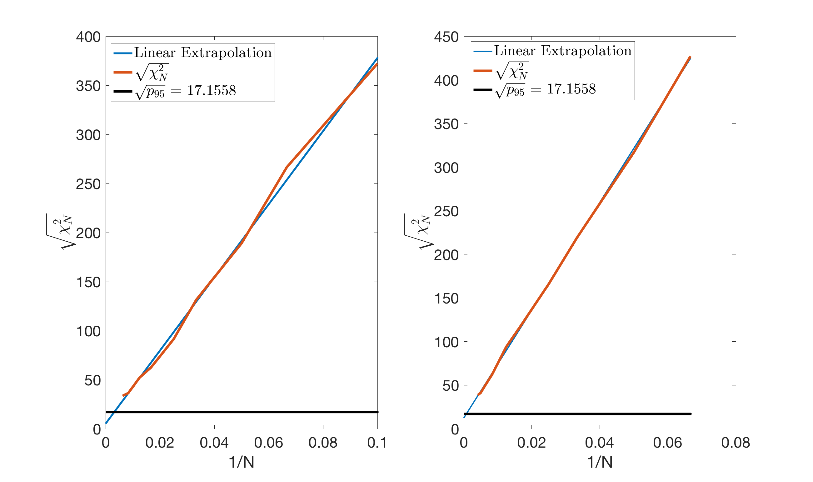
Figure 9. Left: Extrapolation of $\chi^{2}_{N}$ for $\Phi^{1}_{t}$. Right: Extrapolation of $\chi^{2}_{N}$ for $\Phi^{2}_{t}$. Red: $\sqrt{\chi^{2}_{N}}$ vs. $1/N$. Blue: linear extrapolation. Black: $\sqrt{p_{95}}$, square root of the $95$th percentile of the $\chi^{2}$ distribution with $256$ degrees of freedom.

We remark that in order to get the desired accuracy, one needs to efficiently generate large number of samples to approximate the invariant probability measure. This is achieved by using the Hashing-Leaping Method proposed in [15] and parallel computation.

5. Conclusion

In this paper we study a stochastic energy exchange model with two different rate functions that corresponding to different ways of reduction from a deterministic billiards-like heat conduction model. The Markov chain generated by the model with rate function $R_{1}=\sqrt{E_{1}+E_{2}}$ (resp. $R_{2}=\sqrt{E_{1}E_{2}/(E_{1}+E_{2})}$) is denoted by $\Phi^{1}_{t}$ (resp. $\Phi^{2}_{t}$). Two processes have fundamental difference when a low energy site appears. In $\Phi^{1}_{t}$, a low energy site can be quickly “rescued” by its neighbors. However, the rate function of $\Phi^{2}_{t}$ means a low energy site can only be recovered by itself, which usually takes a long time. It is known that this low energy site effect causes the speed of convergence to the invariant probability measure much slower. We are interested in the difference of macroscopic thermodynamic properties caused by this difference. Since an explicit formula of the nonequilibrium steady state (NESS) is not possible, we carry out a series of numerical studies in this paper.

The first study is about the thermal conductivity. We first proved that the thermal conductivity is a well-defined and computable quantity. Our simulations find that both models have thermal conductances that are proportional to $1/N$. This implies a “normal” thermal conductivity that is independent of the system size. In other words, the low energy site effect of $\Phi^{2}_{t}$ does not qualitatively change the thermal conductivity. However, the thermal conductivity is quantitatively reduced by the low energy site effect. This can be verified by comparing the thermal conductivities of 1D and 2D models. In a 2D model the energy transport can bypass the low energy site. Hence an increase of thermal conductivity for $\Phi^{2}_{t}$ is observed in 2D, while the thermal conductivity of $\Phi^{1}_{t}$ is roughly unchanged.

The next study is on the marginal distributions at the NESS, which is related to the existence of local thermodynamic equilibrium (LTE). Our numerical and analytical studies show that when the chain is sufficiently long, for both $\Phi^{1}_{t}$ and $\Phi^{2}_{t}$, the marginal distribution with respect to a non-boundary site approaches to a theoretical thermal equilibrium (Gamma distribution). Additional carefully designed numerical studies reveal that the marginal distribution of nearest neighboring sites also approaches to the product of two independent Gamma distributions regardless of the rate function. However, the low energy site effect of $\Phi^{2}_{t}$ causes the chain to be more “sticky”. As a result, for the same system size, nearest neighbor sites of $\Phi^{2}_{t}$ are more dependent than those of $\Phi^{1}_{t}$.

Understanding the consequence of the “low energy site effect” is an important step in the derivation of macroscopic thermodynamic laws from nonequilibrium billiards-like dynamics. Recall that the stochastic energy exchange model $\Phi^{2}_{t}$ serves as an approximation of the time evolution of the energy profile of a billiard model. In our recent paper [14], we consider many particles that are trapped in the same cell as described in Figure 1. A more realistic stochastic energy exchange model is then derived from simulating this billiard model. A weaker “low energy site effect” is still observed in this stochastic energy exchange model. The new stochastic energy exchange model in [14] is very important because it has a mesoscopic limit equation. Many important macroscopic thermodynamic properties like the Fourier’s law, the long-range correlation, and the fluctuation theorem, can be derived from this mesoscopic limit equation rigorously. Numerical computation in this paper shows that the “low energy site effect” does not qualitatively change key macroscopic thermodynamic properties. This not only answers questions about $\Phi^{2}_{t}$ asked by several researchers in the field, but also makes the ongoing and future study on the new stochastic energy exchange model in [14] more convincing. In this sense, the study in the present paper improves our understanding about how macroscopic thermodynamic laws are derived from microscopic Hamiltonian dynamics.

References

- [1] F. Bonetto, J.L. Lebowitz, and L. Rey-Bellet, Fourier’s law: a challenge to theorists, Mathematical physics 2000 (2000), 128–150.
- [2] Leonid Bunimovich, Carlangelo Liverani, Alessandro Pellegrinotti, and Yurii Suhov, Ergodic systems ofn balls in a billiard table, Communications in mathematical physics 146 (1992), no. 2, 357–396.
- [3] Nikolai Chernov and Roberto Markarian, Chaotic billiards, no. 127, American Mathematical Soc., 2006.
- [4] Nikolai Chernov and Hong-Kun Zhang, Billiards with polynomial mixing rates, Nonlinearity 18 (2005), no. 4, 1527.
- [5] István Fazekas and O Klesov, A general approach to the strong law of large numbers, Theory of Probability & Its Applications 45 (2001), no. 3, 436–449.
- [6] Pierre Gaspard and Thomas Gilbert, Heat conduction and fourier’s law in a class of many particle dispersing billiards, New Journal of Physics 10 (2008), no. 10, 103004.
- [7] by same author, Heat conduction and fourier’s law by consecutive local mixing and thermalization, Physical review letters 101 (2008), no. 2, 020601.
- [8] by same author, On the derivation of fourier’s law in stochastic energy exchange systems, Journal of Statistical Mechanics: Theory and Experiment 2008 (2008), no. 11, P11021.
- [9] A. Grigo, K. Khanin, and D. Szasz, Mixing rates of particle systems with energy exchange, Nonlinearity 25 (2012), no. 8, 2349.
- [10] C. Kipnis, C. Marchioro, and E. Presutti, Heat flow in an exactly solvable model, Journal of Statistical Physics 27 (1982), no. 1, 65–74.
- [11] Stefano Lepri, Roberto Livi, and Antonio Politi, Thermal conduction in classical low-dimensional lattices, Physics reports 377 (2003), no. 1, 1–80.
- [12] Yao Li, On the stochastic behaviors of locally confined particle systems, Chaos: An Interdisciplinary Journal of Nonlinear Science 25 (2015), no. 7, 073121.
- [13] by same author, On the polynomial convergence rate to nonequilibrium steady-states, The Annals of Applied Probability, accepted (2018).
- [14] Yao Li and Lingchen Bu, From billiards to thermodynamic laws: I. stochastic energy exchange model, Chaos: An Interdisciplinary Journal of Nonlinear Science, accepted (2018).
- [15] Yao Li and Lili Hu, A fast exact simulation method for a class of markov jump processes, The Journal of chemical physics 143 (2015), no. 18, 184105.
- [16] Yao Li, Péter Nándori, and Lai-Sang Young, Local thermal equilibrium for certain stochastic models of heat transport, Journal of Statistical Physics 163 (2016), no. 1, 61–91.
- [17] Yao Li and Lai-Sang Young, Existence of nonequilibrium steady state for a simple model of heat conduction, Journal of Statistical Physics 152 (2013), no. 6, 1170–1193.
- [18] C Mejia-Monasterio, H Larralde, and F Leyvraz, Coupled normal heat and matter transport in a simple model system, Physical review letters 86 (2001), no. 24, 5417.
- [19] K Ravishankar and Lai-Sang Young, Local thermodynamic equilibrium for some stochastic models of hamiltonian origin, Journal of Statistical Physics 128 (2007), no. 3, 641–665.
- [20] Makiko Sasada, Spectral gap for stochastic energy exchange model with nonuniformly positive rate function, The Annals of Probability 43 (2015), no. 4, 1663–1711.
- [21] Nándor Simányi, Proof of the boltzmann-sinai ergodic hypothesis for typical hard disk systems, Inventiones Mathematicae 154 (2003), no. 1, 123–178.
- [22] Nándor Simányi and Domokos Szász, Hard ball systems are completely hyperbolic, Annals of Mathematics 149 (1999), 35–96.