Predicting the COSIE-C Signal from the Outer Corona up to 3 Solar Radii.

Abstract

We present estimates of the signal to be expected in quiescent solar conditions, as would be obtained with the COronal Spectrographic Imager in the EUV in its coronagraphic mode (COSIE-C). COSIE-C has been proposed to routinely observe the relatively unexplored outer corona, where we know that many fundamental processes affecting both the lower corona and the solar wind are taking place. The COSIE-C spectral band, 186–205 Å, is well-known as it has been observed with Hinode EIS. We present Hinode EIS observations that we obtained in 2007 out to 1.5  $\rm R_{\odot}$, to show that this spectral band in quiescent streamers is dominated by Fe xii and Fe xi and that the ionization temperature is nearly constant. To estimate the COSIE-C signal in the 1.5–3.1  $\rm R_{\odot}$ region we use a model based on CHIANTI atomic data and SoHO UVCS observations in the Si xii and Mg x coronal lines of two quiescent 1996 streamers. We reproduce the observed EUV radiances with a simple density model, photospheric abundances, and a constant temperature of 1.4 MK. We show that other theoretical or semi-empirical models fail to reproduce the observations. We find that the coronal COSIE-C signal at 3  $\rm R_{\odot}$ should be about 5 counts/s per 3.1″ pixel in quiescent streamers. This is unprecedented and opens up a significant discovery space. We also briefly discuss stray light and the visibility of other solar features. In particular, we present UVCS observations of an active region streamer, indicating increased signal compared to the quiet Sun cases.

1. Introduction

It is now quite well established that the outer corona, i.e. the region between 1.5 and 3  $\rm R_{\odot}$ (as measured from Sun center) is the place where many fundamental processes are taking place. For example, this is the region where the solar wind and the Coronal Mass Ejections (CME) become accelerated, see e.g. Abbo et al. (2016); Zhang & Dere (2006); Temmer et al. (2017). This is also the region where CME driven waves steepen into shocks, and as the Alfven Mach number increases from 1, the post shock plasma in a CME can transition from low beta to high beta.

The outer corona is also the region where the small-scale complex topology of the magnetic field, which shapes the observed features of the lower corona, becomes more simple and radial. It is also a transition region from collisional fluid to collisionless plasma.

The outer corona could also contain, depending on which model one considers, the transition region from the low-$\beta$ collisional inner corona to the high-$\beta$ collisionless heliosphere and the nascent solar wind. For example, Fig. 6 of the MHD model of Vásquez et al. (2003) shows that $\beta=1$ around 2 $\rm R_{\odot}$ in a streamer, while $\beta$ in a coronal hole is very small out to the edge of the plot at 4  $\rm R_{\odot}$. Other models put the $\beta=1$ further out, closer to the Alfven point.

The outer corona is also the region where processes such interchange reconnection between closed and open structures is likely taking place, even in the quiet Sun (see, e.g. Fisk, 2003). The complex mix of quiet Sun areas and coronal holes creates a complex topological system. MHD simulations of the quiet corona around the time of the 2008 eclipse run by the Predictive Science group with the MAS code Mikić et al. (2007) showed the presence of a multitude of separators and quasi-separatrix layers in the outer corona, which have a profound effect on the magnetic connectivity between a point in the heliosphere and its source region, the so-called S-web (Antiochos et al., 2011).

When even a single active region is present, the topology of the global magnetic field of the outer corona becomes more complex. For example, magnetic field modeling of a few isolated active regions observed in 2007 showed the presence of null points at about 2  $\rm R_{\odot}$ (Del Zanna et al., 2011a). A model of interchange reconnection taking place at these null points was able to reproduce the location and strength (see also Bradshaw et al., 2011) of the so-called ‘coronal outflows’, regions mostly connected to sunspots that show upflowing plasma at temperatures above 2 MK (see, e.g. Del Zanna, 2008; Harra et al., 2008; Doschek et al., 2008). This interchange reconnection process in active regions is in principle capable of injecting coronal plasma that was originally present in the closed hot (3 MK) loops of active region cores into the heliosphere, and forming as a by-product the large-scale cooler (1 MK) loops which fan out of sunspots and connect to the entire surroundings of an active region.

It is clear that the density at 2  $\rm R_{\odot}$ is so low that whatever occurs at 2  $\rm R_{\odot}$ is virtually invisible in on-disk observations, against the bright background of the inner corona. Therefore, off-limb high-resolution observations around 2  $\rm R_{\odot}$ are needed. Yet, this region is relatively unexplored, with the exception of a few ground-based observations during total eclipses, and SoHO/UVCS (Kohl et al., 1995) spectra. Such observations returned plenty of scientific results, but were not capable of monitoring the dynamical evolution of the outer corona.

Narrow-band high-resolution images of the solar corona in the visible taken during total eclipses have shown us the outer corona in its full glory, with many complex open and closed structures, and features that are difficult to comprehend. For example, intriguing features have appeared in recent images of the Fe xi visible forbidden line (Habbal et al., 2011). Such images of the coronal lines show more clearly the outer structures not only because of the natural occulter (the Moon), but also because the intensities of the visible forbidden lines decay more slowly with height, compared to the allowed lines. This occurs partly because forbidden line intensities decay linearly with the electron density, and partly because the photospheric radiation increases their intensities via photo-pumping (see, e.g. Del Zanna & DeLuca, 2018, for a recent discussion of visible and infrared forbidden lines). Unfortunately, these eclipse images are very short snapshots of a corona that we know is highly dynamic.

Above 2  $\rm R_{\odot}$, coronagraphic observations in the visible with e.g. the SoHO Large Angle Spectroscopic COronagraph (LASCO) C2 (Brueckner et al., 1995), and further out from STEREO HI, have provided valuable information about the dynamic outer corona. However, the spatial resolution and sensitivity have not been comparable with ground-based eclipse observations. Future coronagraphs in the visible (e.g. Proba-3, Aditya) will provide significant improvements, but such instruments will always be limited by the fact that the coronal signal is more than 6 orders of magnitude weaker than the photospheric one. The Solar Orbiter Metis coronagraph will be an improvement on the current situation as it will provide images both in the visible and in the UV, in the hydrogen Ly $\alpha$ above 1.6  $\rm R_{\odot}$. The Solar Orbiter EUI full-disk images are in principle also capable of observing the outer corona, but outside the currently planned remote-sensing windows (during close encounter).

Around 2  $\rm R_{\odot}$, we had only a few images of the outer corona. LASCO/C1 observed the outer corona up to 3 $\rm R_{\odot}$ in the green and red visible forbidden lines, but returned only limited results (see, e.g. Mierla et al., 2008). We have plenty of observations from the X-rays to the UV of the lower corona in a range of spectral lines and broad-bands, typically up to 1.3  $\rm R_{\odot}$, but the nearly exponential decay of the electron density with radial distance, typical of stationary isothermal plasma, reduces dramatically the XUV signal, as the intensities of dipole-allowed transitions are proportional to the square of the electron density.

There are a few off-points from SDO AIA (mainly for comet observations) where we see structures in the EUV out beyond 2 $\rm R_{\odot}$. Recently, also SUVI obtained some off-limb images. We also have PROBA2/SWAP EUV images (in a band around 174 Å dominated by Fe x and Fe ix) which clearly show a very complex and dynamical behavior of open and closed structures, especially above active regions. The dynamical behavior is mainly seen in the SWAP Carrington movies. The effects of an emerging AR are also clearly evident in AIA, see e.g. Schrijver & Higgins (2015).

To overcome the lack of detailed information about the outer corona, an instrument of novel design has recently been proposed to fly on the International Space Station: the COronal Spectrographic Imager in the EUV (COSIE). The instrument has two modes of operation. The spectrograph mode will mainly be used on-disk: it is a full Sun slitless imaging spectrograph (COSIE-S). The other one is a broad-band imager which will mainly be used in its coronagraphic mode (COSIE-C), although it can also observe on-disk, with a filter to reduce the bright on-disk signal.

The key issue here is that building a coronagraph in the visible has always been a challenge, given the huge dynamic range between the disk intensity and the signal of the outer corona. This is not the case in the EUV, so an instrument such as COSIE can naturally observe both on-disk and off-limb.

In a nutshell, COSIE-C is designed to observe the corona in an EUV spectral band between 186 and 205 Å with a high-cadence, a large field of view (FOV) of 6.6 $\rm R_{\odot}$ $\times$ 6.6 $\rm R_{\odot}$, and a spatial resolution of 3.1″. Such a resolution is really high, when compared to previous coronagraph images, and comparable to that of many current EUV instruments observing on-disk, such as Hinode EIS. This spectral range is well-known, as it has been routinely observed with many previous and current space-based instruments such as SoHO/CDS, SoHO/EIT, TRACE, STEREO/SECCHI, SDO/AIA, SDO/EVE, GOES SUVI. In particular, detailed spectroscopic observations with Hinode/EIS have been studied in detail, and over the past years all the main lines have been identified, and the atomic data has been recalculated and benchmarked, as reviewed in Del Zanna (2012). The quiet solar corona (at about 1 MK) is emitting in this spectral region strong coronal lines from iron ions: Fe x, Fe xi, and Fe xii.

The main aim of the coronagraphic mode of COSIE is to provide continuous monitoring of the outer corona with high-cadence and sensitivity, so dynamic events such as CME or waves in the outer corona can be studied in detail.

In order to achieve this, a key technical issue regards the ability to observe simultaneously the inner corona from the solar limb to the outer corona. In principle the instrument is capable of observing up to 4.6  $\rm R_{\odot}$ from Sun center, along the diagonal of its square FOV of 6.6$\times$6.6  $\rm R_{\odot}$, however as we have discussed the most interesting (and relatively unexplored) region of the solar corona is between 1.5 and 3.3  $\rm R_{\odot}$  which is what will be observed within the square FOV of COSIE.

The main aim of the present paper is therefore to provide observational evidence of how the brightness of the EUV corona changes with radial distance from the Sun in the 1.5–3  $\rm R_{\odot}$ range, so we can provide relatively accurate estimates of the COSIE signal up to these distances. We mainly consider quiet Sun streamers in this paper as they are much less variable than e.g. those above active regions, or signals in other features. However, we provide one example of the signal above an active region streamer, and provide some comments of what signals could be expected for other regions.

Our main aim might seem relatively simple, from an observational or modeling perspective, but it is not, as we discuss here. We know, from past observations, that the intensity of the disk in the EUV is comparable with the intensity of the inner corona as observed off-limb, but the behavior of the coronal lines up to about 3  $\rm R_{\odot}$ was not known until the present study. Within the literature, we have not found direct measurements of coronal lines up to 3  $\rm R_{\odot}$ in the quiet Sun. The only study of the outer corona is that by Goryaev et al. (2014), where however a streamer above an active region was observed. PROBA2/SWAP images in the 174 Å band were analyzed up to 2  $\rm R_{\odot}$. The broad-band signal decreased by about 3 orders of magnitude in this range. Interestingly, a nearly isothermal corona of 1.4 MK was needed to explain the observations, as we have also found here.

In principle, we could supplement the lack of observations with modeling. However, being an unexplored region, we really do not know how the fundamental plasma parameters vary with radial distance. Even considering the most simple case of a streamer in the quiet Sun, very different estimates of densities and temperatures have been published. A few are shown in Figure 1, together with those we have adopted for our modeling, as described below.

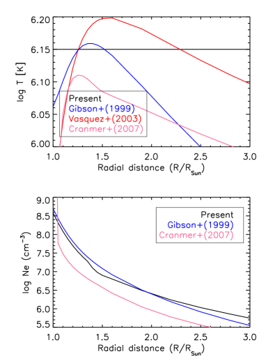
Figure 1.— The radial profiles of the electron densities and temperatures we assumed for modeling quiet Sun streamers (black lines), compared to some literature values.

Such variable densities and temperatures produce very different estimates of coronal line radiances, as discussed in Andretta et al. (2012) and as also shown here. Furthermore, an issue which greatly complicates any modeling effort is the variability of the elemental abundances, as we discuss below.

An ideal instrument which explored the outer corona is SoHO/UVCS because it observed many coronal lines formed at similar temperatures as those that contribute to the COSIE-C band. There are, of course, many published results from SoHO/UVCS (and the previous similar SPARTAN instrument) which observed the outer corona from 1996 even as far as 10  $\rm R_{\odot}$. However, the instrument sensitivity was such that only the brightest lines, the H I Lyman $\alpha$ and the O vi doublet, had enough signal in the outer corona. These lines are largely affected by photoexcitation as the density of the outer corona decreases, so they are visible to greater distances, but are not ideal to estimate the signal in the collisionally-dominated EUV lines, as we will discuss below.

There are many published results from UVCS, where several coronal EUV lines were observed. However, they were mostly at distances of about 1.5  $\rm R_{\odot}$, see e.g. Raymond et al. (1997); Parenti et al. (2000). We have therefore searched the UVCS database to try and find some observations that could be useful for our purpose. We have identified a few observations of the Mg X and Si XII coronal lines in the 1.4–3  $\rm R_{\odot}$ range, which we could use to build a model to estimate the COSIE Iron line count rates in the 186–205 Å range. Several new and interesting results are obtained from this analysis. At lower heights, we present the analysis of a unique Hinode EIS off-limb observation where coronal lines (the same that would be observed by COSIE) were visible up to 1.5  $\rm R_{\odot}$.

The paper is organized as follows: Section 2 describes the UVCS observations of quiescent streamers and their analysis. Section 3 describes the way we have modeled the UVCS observed radiances, and the predictions we make for the COSIE-C signal in the outer corona. Section 4 briefly discusses the EIS off-limb observation, while Section 5 briefly discusses stray light issue. Section 6 provides some comments on the expected COSIE-C signal in other regions and features, while Section 7 draws the conclusions.

2. Quiet Sun UVCS Observations and data analysis

During 1996 and early 1997, the Sun was relatively quiet, with the exception of a few small active regions, and a long-lived large one, located in the southern hemisphere, at the end of a large, long-lasting trans-equatorial coronal hole, the ‘Elephant’s trunk’ (Del Zanna & Bromage, 1999).

During this period, the UVCS instrument was routinely running synoptic studies, where the corona between about 1.4 and 3.5 $\rm R_{\odot}$was observed by moving the slit in 4-5 different radial locations and then rotating the slit around the Sun. Coronagraph and UVCS observations during this period clearly show how the streamers are affected by the presence of these different structures, especially active regions. A review summary of the UVCS observations in the H I and the O VI lines during this period can be found in Antonucci et al. (2005).

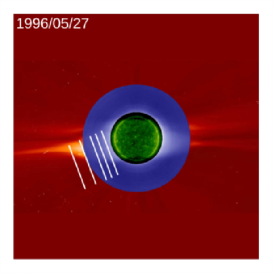
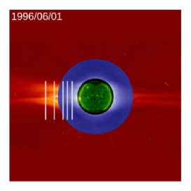
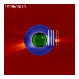
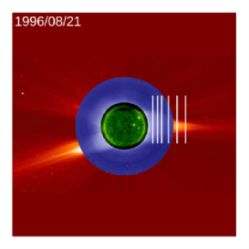
Figure 2.— Composite images including SoHO EIT 195 Å, HAO Mauna Loa Mark 3 and LASCO/C2 white-light coronagraphs during times when the quiescent streamers discussed here were observed by SoHO UVCS, on 1996 May 27 (top left) and 1996 August 19 and 21 (bottom). The top right plot shows an active region streamer observed on 1996 June 1. The location of the UVCS slit is shown.

However, these UVCS synoptic observations typically had narrow slits and exposure times of 500 or 1,000 seconds, generally too short to get enough signal in the coronal lines above 2 $\rm R_{\odot}$. We have therefore searched the entire UVCS database of the first year of operation, to try and find observations of quiescent streamers with slit positions up to 3  $\rm R_{\odot}$ and exposures long enough so we could measure the radiances of the coronal lines. We have visually inspected dozens of observations and at the end only found a few useful datasets. Figure 2 shows the streamers we selected for further analysis. One was a quiet streamer observed on 1996 May 27. During the following 28-day solar rotations, on June 24, July 22, and August 19, the streamer became increasingly active, because of the emergence of the large active region connected to the Elephant’s trunk which we have mentioned. On the other hand, on the opposite side of the Sun, the other (west) streamer was very quiescent for at least several days, around August 19. Indeed this streamer has previously been studied by several authors. In particular by Gibson et al. (1999), where the polarized Brightness (pB) measured by the HAO Mauna Loa Mark 3 and LASCO/C2 white-light coronagraphs was used to infer electron densities. We have analyzed the observations on August 19th and 21st of the same streamer, to see if there were significant changes. We found very little difference in the radiances, confirming the impression from the LASCO/C2 images of a stable streamer. Figure 2 also shows one active region streamer, observed on 1996 June 1, and discussed below.

We have used the fully-calibrated UVCS data as available via the Virtual Solar Observatory. We have used the latest version 5.2 of the UVCS software (DAS) to sum the exposures and obtain the calibrated data. We have considered the O VI primary channel, where the O VI doublet, the H i 1025 Å and the Si xii 521 Å (in second order) lines are present. We have also analyzed the redundant O VI channel, where the Mg x 610 Å line is present in second order, next to the hydrogen Ly $\alpha$.

We have then averaged the line radiances over the regions where the lines were clearly visible, in order to increase the signal-to-noise of the very weak coronal lines. This clearly averages the variations that have been reported between the streamer cores and the boundaries, especially in terms of elemental abundances (Raymond et al., 1997). However, we had no choice, considering that further out, above 2  $\rm R_{\odot}$, the streamers become very narrow and it becomes difficult to try and measure the core and the boundary regions. Also, line of sight effects mean that boundary regions are always intermixed with core regions. We have carefully measured the line radiances by subtracting a linear background in each spectrum with custom-written software by one of us (GDZ).

The calibrated UVCS data assume a first-order calibration. The UVCS radiometric calibration for first order lines was measured before launch and tracked in flight by observing UV-bright stars. Such calibration was not possible for second order lines, so we rely on laboratory measurements of the reflectivities of the mirror materials, the efficiency of a similar grating, and sensitivity of KBr coated detector at the Mg X and Si XII wavelengths. The cumulative uncertainty on the measured radiances is difficult to estimate, but it is probably about 30–40%. Now that the SOHO CDS has a reliable long-term radiometric calibration (Del Zanna & Andretta, 2015), it is in principle possible to cross-calibrate UVCS against CDS, especially considering that the same spectral lines were observed during some targeted campaigns. We have identified some useful datasets, but leave such a complex analysis for a future paper. For this paper, we have applied the following scaling factors to the second-order lines: 0.14 for the Si xii 521 Å line and 0.27 for the Mg x 610 Å line in the redundant channel. These factors have been widely used in the past literature and an uncertainty of 40% is reasonable for the purposes of the present paper.

The measured radiances are shown in Figures 3,4. The differences between the radiances of the west streamer, observed on the 19th and 21st, are small. What is remarkable is the agreement in the radiances of the east streamer, indicating very little differences between the two streamers during this quiet period. It is also remarkable that the radiances of the two coronal lines decrease by only about two orders of magnitude between 1.5 and 3.1  $\rm R_{\odot}$.

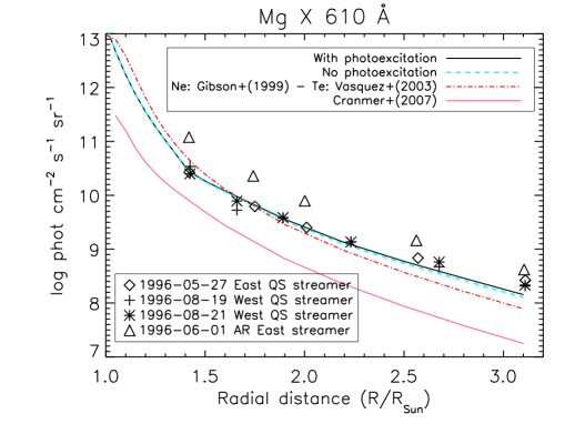
Figure 3.— The radiance of the Mg x 610 Å line as a function of the radial distance, for three quiet Sun (QS) observations and one active region (AR). The lines are the predicted radiances.

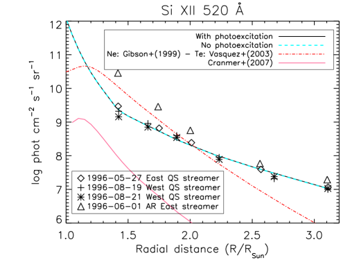
Figure 4.— The radiance of the Si xii 521 Å line as a function of the radial distance for three quiet Sun (QS) observations and one active region (AR). The lines are the predicted radiances.

3. Modeling the UVCS observations of the quiet Sun streamers and use them for COSIE-C

For our analysis and simulations we used the atomic data from CHIANTI (Dere et al., 1997) in its version 8 (Del Zanna et al., 2015).

Given the simple structure of the streamers, we adopted a similar approach as that one we adopted in Andretta et al. (2012), where off-limb radiances of a selection of coronal lines and the He II resonance line were modeled. The approach is very common in the literature: it consists of adopting a uniform radial dependence of the electron density and temperature, estimating the line emissivities, and then integrating along each line of sight assuming cylindrical symmetry. In our simulations, we calculated line emissivities up to 10  $\rm R_{\odot}$, then performed the integrations until a radial distance of 3.1  $\rm R_{\odot}$. For each line of sight, we integrated up to a distance of 9  $\rm R_{\odot}$, although the main contribution to the emission comes from the region closest to the Sun. This simple approach works very well in reproducing the radiances of the collisional lines, which is the main aim of the present modeling. This approach is also justified by several considerations, as discussed by Frazin et al. (2003), where UVCS observations of another quiescent streamer were analyzed. However, we are exploring various other geometrical and density/temperature distributions for a future paper, as the current model is unable to reproduce the observations of the radiatively excited lines, see below.

Since version 4 of the CHIANTI database (Young et al., 2003), it is possible to introduce photoexcitation into the modeling of line emissivities. We used such an option with a few modifications by one of us (GDZ) to the software. The model assumes a uniform source of disk radiation, and calculates the excitation rate at each distance by including a dilution factor, which depends on the distance from the Sun. We originally provided an input quiet Sun spectrum, covering all wavelengths from the X-rays to the infrared. However, the electron densities of our models are so low that the ‘coronal model’ approximation holds: all the population is in the ground states and the metastable levels are not populated. Therefore, only the disk photoexcitation at the wavelength of the spectral line of interest is needed. In the results shown here, we have assumed that the disk radiation is monochromatic and has the wavelength of the spectral line.

However, we have also calculated the photo-pumping by providing a disk emission profile and an absorption one, to study Doppler dimming effects. Given the large Doppler widths of the coronal ions, the disk emission is totally absorbed in the absence of strong outflows, so the two approaches are fully equivalent.

Doppler dimming effects can become important, if strong outflows are present (see, e.g. Noci et al., 1987). In general, when outflows are present, the photo-pumping disk radiation becomes Doppler-shifted so the photoexcitation (and consequently the line intensity) decreases, although photo-pumping from nearby lines can occur, as in the O VI case, also discussed by Noci et al. (1987). There is ample observational evidence that quiescent streamer axes are characterized by negligible outflows (at most a few km/s) for the distances we are concerned here (see, e.g. Strachan et al., 2002; Frazin et al., 2003; Uzzo et al., 2006; Noci & Gavryuseva, 2007; Spadaro et al., 2007).

Other assumptions we have made are that lines are optically thin, and that the electron temperatures are the same as the proton and ion temperatures, and the plasma is in ionization equilibrium. That the electron and proton temperatures should be nearly equal is supported by the observation that the width of the H I Lyman $\alpha$ line is close to the ionization temperature as measured by e.g. line ratios. The ionization temperature is equal to the electron one, assuming equilibrium, and the temperature of the neutral hydrogen must be close to the proton temperature. The assumption of ionization equilibrium is also common and is justified by the absence of any measurable flows, and the relatively high densities. This assumption is clearly untenable in coronal hole regions, where strong outflows of hundreds of km/s and much lower densities than in our QS streamers have been routinely measured by UVCS. We note that Shen et al. (2017) computed the effects of time-dependent ionization in a pseudo-streamer out to 3  $\rm R_{\odot}$  based on an MHD model. For that particular model, time-dependent ionization increases the Mg X intensity because the temperature declines with height.

Having established the method, a further problem has been how to choose which parameters one should adopt. We discuss below disk radiation, electron densities, elemental abundances and electron temperatures.

The accurate assessment of the disk radiation is a non-trivial issue, as different instruments have provided different measurements, and as radiances of all the lines we are concerned here have a strong variation with the solar activity (see the discussion in Del Zanna & Andretta, 2015). For the Mg x 610 Å line we have adopted a value of 110 erg cm^-2 s^-1 sr^-1 from OSO observations, and for the Si xii 521 Å line 19 erg cm^-2 s^-1 sr^-1. However, we found that photoexcitation for these two coronal lines has a totally negligible effect on the line intensities for the present model.

As discussed in Andretta et al. (2012), there is a wide range of density and temperature models for quiescent streamers, each of them producing very different results. The beauty of the EUV/UV spectroscopy provided by UVCS is that the observed spectral lines are extremely sensitive to any small variation in these parameters, hence provide an excellent test to these models.

The parameter that is better measured is the electron density. During the first two years of the SoHO mission, one of us (GDZ) obtained a large number of off-limb observations and monitored the off-limb density using line ratios (Del Zanna, 1999; Fludra et al., 1999). The above-mentioned near-simultaneous measurements of the pB produced densities in relative good agreement with those measured by CDS, for the August 19 west streamer (Gibson et al., 1999). We therefore used as a baseline for our modelling these densities, although some minor changes, shown in Figure 1, were applied to improve agreement in the radiances of the Mg x and Si xii observed by UVCS. In the same figure we also show the modeled densities for an equatorial quiet Sun by Cranmer et al. (2007), which have been widely used in the literature. Note that the paper is mostly focusing on modelling coronal holes, but also provides other models. We have used the data file cvb07_equator.dat for an equatorial streamer at solar minimum.

We note, however, that an analysis of the same streamer by Antonucci et al. (2005), based on the ratios of the two O VI lines, produced significantly lower densities. That some differences in the densities occur should not be surprising. For example, the Thompson scattered Pb signal is proportional to the density, while the collisionally-dominated coronal line intensities are proportional to the square of the density. Therefore, if the plasma is not uniformly distributed in density, some changes could occur. However, the issue is more complex, as we briefly describe below.

Another parameter which affects the modelling is the elemental abundance. It is well-known that remote-sensing observations of the solar corona, from the visible to the X-rays, have shown that coronal abundances can be different from the photospheric ones, and that correlations exist between the abundance of an element and its first ionization potential (FIP). The low-FIP ($\leq$ 10 eV) elements are more abundant than the high-FIP ones, relative to their photospheric values. On the other hand, usually the relative abundances among elements with similar FIP do not vary. Similar FIP bias variations are observed in-situ in the slow solar wind. See, e.g. the Living Reviews by Laming (2015) and Del Zanna & Mason (2018) for details.

Since the COSIE band is dominated by lines from coronal iron ions, and we use the Si xii and Mg x radiances measured by UVCS for the estimates, the choice of the elemental abundances is irrelevant, considering that Si, Mg, and Fe are all low-FIP elements, so their relative abundances are not expected to vary much.

For our modelling, we took the simplest approach. Considering that we averaged over the entire sections of the streamers, we are not able to assess differences between the core and the outer parts of the streamers, although the emission primarily comes from the brightest regions, the legs. We therefore took as a baseline the photospheric abundances of Asplund et al. (2009), considering that there is evidence (although still debated in the literature) that the inner quiescent corona (around 1 MK) has nearly photospheric abundances, within a factor of two. This has been obtained by comparing S and Fe coronal lines observed by Hinode EIS (Del Zanna, 2012), and a wide range of elements in a recent reanalysis of off-limb SOHO SUMER observations (Del Zanna & DeLuca, 2018).

The parameter that is virtually unknown is the electron temperature. Gibson et al. (1999) obtained the temperatures shown in Figure 1 assuming an hydrostatic atmosphere. As shown below, they produce radiances in the coronal lines that decrease with radial distance far more than observations, so we have discarded them. A much better model is the semi-empirical one developed by Vásquez et al. (2003). It was based on the widths of the H I Lyman $\alpha$ line, measured by UVCS, with the assumption that the electron and proton temperatures are the same in the streamers, where the plasma is expected to be in thermal equilibrium. However, after some tests, also this model was unable to reproduce our UVCS observations. Another temperature profile shown in the same figure is the modeled one for an equatorial quiet Sun by Cranmer et al. (2007).

We would like to point out that we are not interested here in the real electron temperature, but rather in the temperature which, assuming ionization equilibrium, does fit the observed radiances in the coronal lines. This is in practice a ionization temperature. It is well-known (see, e.g. Del Zanna, 1999; Fludra et al., 1999) that the ratio of the Si xii and Mg x Li-like lines is an excellent temperature diagnostic which is not affected by variations in density nor in elemental abundances (as both elements have a low-FIP).

We have measured the ionization temperature using the UVCS measurements and found it to be remarkably constant around log $T$ [K] =6.15. Any temperature decrease would have a dramatic effect on the hotter Si xii line, which would decrease significantly. We have therefore assumed this temperature, keeping in mind that the actual value is dependent on the accuracy of the relative calibration of the two UVCS channels where the two lines are observed. It interesting to note that in the inner corona, up to 1.3  $\rm R_{\odot}$, there is spectroscopic evidence from SOHO CDS (see, e.g. Del Zanna, 1999; Andretta et al., 2012) and SOHO SUMER (see, e.g. Landi & Feldman, 2003) that the ionization temperature is normally nearly constant. We provide below further evidence from one Hinode EIS observation that the ionization temperature is nearly constant up to 1.5  $\rm R_{\odot}$. Any variation of the density and temperature above 3  $\rm R_{\odot}$ does not significantly affect the modelling.

The predicted intensities are shown in the plots, together with the measured radiances. Excellent agreement is found for the Si xii and Mg x coronal lines.

3.1. On the radiatively-excited lines and the chemical abundances

As the H i Lyman $\beta$ 1025 Å  line is largely collisional (at least at closer distance), we have also predicted its radiances, which allow us to measure the absolute abundances of Mg and Si in these observations.

One of the many stunning results from UVCS was the discovery of very unusual abundances in the cores of quiescent streamers, with high-FIP elements such as O being depleted by about an order of magnitude, compared to its photospheric value (see e.g. Raymond et al., 1997, and following papers). The low-FIP elements such as Si and Mg also appeared depleted, but by not as much. These abundance measurements have usually been obtained by comparing the line radiances with the radiance of the H I Lyman $\alpha$, with some assumptions and modelling. In particular, by considering separately the collisional and radiative component of the lines. Such low abundances are anomalous, as they are not observed in the lower corona, though they are sometimes seen in the solar wind (Weberg et al., 2012, 2015).

A possible interpretation is mass-dependent settling, which was observed with SOHO SUMER (see Feldman et al., 1998). Furthermore, abundances have been found to vary spatially not only across but also along streamers. Antonucci et al. (2006) analyzed UVCS observations of the H I and the O VI lines and found a variation in the O abundance in the regions surrounding the quiescent solar minimum streamers. Uzzo et al. (2003) analyzed the UVCS observations of the streamer belt from 1996 June 1 to August 5 to study the variation of the elemental composition. Large variations between the streamers cores and legs were confirmed, as well as variations between streamers.

For the H i Lyman $\beta$ 1025 Å  line we used a disk radiance of 800 (ergs cm^-2 s^-1 sr^-1) as measured by UVCS (Raymond et al., 1997), noting that it is very close to the SUMER QS measurement during the same period of low solar activity reported by Wilhelm et al. (1998) of 766. There are no significant center-to-limb changes in the H I Lyman $\alpha$ line, so we have assumed that the radiance of the Lyman $\beta$ line is constant across the disk.

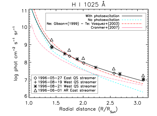
Figure 5.— The radiance of the H i 1025 Å  line as a function of the radial distance for three quiet Sun (QS) observations and one active region (AR). The lines are the predicted radiances.

Figure 5 shows that its predicted radiances are very close to the observed ones indicates that the Mg and Si abundances are close to photospheric.

We note that Raymond et al. (1997) found that in a streamer leg at 1.5  $\rm R_{\odot}$ the Mg and Si abundances were lower than photospheric. For Mg, they found an abundance of 2.5$\times 10^{-5}$, compared to the photospheric value of 4.0$\times 10^{-5}$ we adopted here. For Si, they found a value of 1.25$\times 10^{-5}$, compared to a photospheric value of 3.2$\times 10^{-5}$. On the other hand, Raymond et al. (1997) found the Fe abundance to be photospheric, i.e. 3.2$\times 10^{-5}$. We note that several iron lines were observed, and the abundances were estimated assuming an isothermal temperature of log $T$[K]=6.2, obtained from the relative abundances of the iron lines: Fe xiii, Fe xii, Fe x. Therefore, the results concerning the iron lines should in principle be more reliable, although significant improvements in the atomic data for the Fe xii, Fe x forbidden lines have occurred (see Del Zanna et al., 2012b, a, 2014). These improved data have been distributed in CHIANTI version 8 (Del Zanna et al., 2015). Other authors (cf. Parenti et al. 2000) have found that, on average, the abundances of low-FIP elements in quiescent streamers are nearly photospheric, within a factor of two.

There is however a caveat to these results, i.e. the fact that lines such as the H i Lyman $\beta$ that are partly photo-excited are very sensitive at further distances not only to the disk radiation and outflows (via Doppler dimming), but especially to how the electron density is distributed along the line of sight. Their dependence would be different than that of the collisionally-dominated lines such as Si xii and Mg x, and also different than the pB in the visible continuum. The results at longer distances are dependent on the model because of the stronger photoexcitation contribution to the H i Lyman $\beta$ line, but those around 1.4  $\rm R_{\odot}$ are nearly independent from the photoexcitation.

With our present simple model we were able to find agreement with the H i Lyman $\beta$ and the coronal lines, but not with the observed radiances of the H i Lyman $\alpha$ and the O vi lines. Discrepancies in the O vi lines have been reported previously (see, e.g. Frazin et al., 2003; Antonucci et al., 2005; Spadaro et al., 2007) and could be due to several factors.

As this interesting issue is well beyond the scope of the present paper, we defer it to a future study. We stress here that these issues are of importance for our interpretation of UVCS observations, but are completely irrelevant for the main aim of the present paper. In fact, regardless of how the UVCS coronal lines are modeled, once they are well reproduced, we can then predict very accurately the signal in COSIE-C, as described below.

3.2. Modelling the COSIE-C coronal emission

Modelling the coronal signal expected from COSIE-C is straightforward. Having established that the coronal lines have negligible increases due to photoexcitation up to 3  $\rm R_{\odot}$, we have therefore used the same procedure applied to model the UVCS coronal lines to model the COSIE-C ones. As the main lines contributing to the band for the quiet Sun case are from Fe viii, Fe ix, Fe x, Fe xi, Fe xii, and Fe xiii, we have only calculated the emissivities of these ions. Clearly, if e.g. a CME will enter the field of view, more counts will be produced not only because of the higher densities, but also because of the contributions of other cooler lines in the band. As Fe is a low-FIP element as Mg and Si, and as these iron ions are formed at the same temperatures as the Si xii and Mg x lines, the estimate should be accurate.

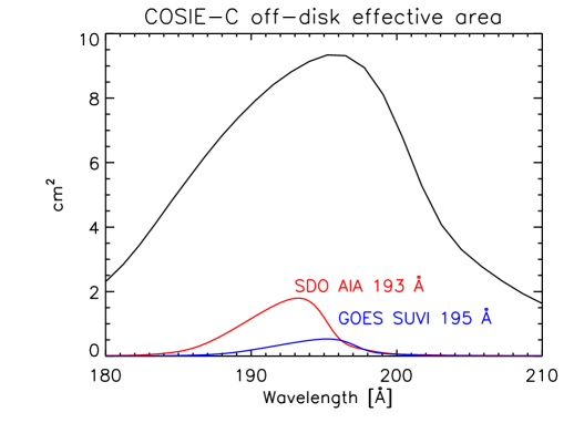
Figure 6.— The estimated COSIE-C effective area, compared to those of the SDO AIA 193 Å and GOES SUVI 195 Å.

We have then folded the expected radiances $I_{\rm r}$ (integrated along the line of sight) with the response of the COSIE-C instrument to estimate the signal $S$ (data numbers per second, DN/s) for a COSIE-C pixel as follows:

$$S=I_{\rm r}\,A_{\rm e}\,{12398.5\over 3.65\,\lambda\,G}\,\Omega$$ (1)

where the terms convert the number of electrons produced in the CCD by a photon of wavelength $\lambda$ (Å) into data numbers DN ($G$ is the gain of the camera), $\Omega$ is the solid angle of one COSIE pixel (3.1″$\times$ 3.1″), and $A_{\rm e}$ is the effective area:

$$A_{\rm e}=\,A\,T_{\rm Al}\,R_{\rm fm}\,R_{\rm m}\,T_{\rm fp}\,{\rm QE}\,$$ (2)

where $A$ is the geometrical area of the telescope (110 cm² with the current design), $T_{\rm Al}$ is the transmission of the Al front filter, $R_{\rm fm}$ is the reflectivity of the front folding mirror, $R_{\rm m}$ is the reflectivity of the main mirror, $T_{\rm fp}$ is the transmission of the internal focal plane filter, and QE is the quantum efficiency of the detector.

As a guideline, we have used for $T_{\rm Al}$ a standard Al front filter with an anti-oxidant layer, similar to the Hinode EIS flight front filter, but with an improved supporting mesh (95% transmission), instead of the one used for EIS (85% transmission). The improved mesh has been flown several times, e.g. for the Hi-C rocket flights (see, e.g. Kobayashi et al., 2014). The total transmission is nearly 60%. For $R_{\rm fm}$ we have used an estimate for a Zr/Al mirror, resulting in about a 65% reflectivity across the wavelength range. For $R_{\rm m}$ we have used the measured reflectivity of the Si/Mo multilayer used for the flight Hinode EIS short-wavelength channel, which has a peak of 35% around 195%. For the focal plane filter we have assumed again an Al filter with a supporting mesh. As the guideline detector should be an improved version of the CCD used for Hinode EIS, we have used a QE=0.8, based on measurements of CCDs with enhanced backside treatments (note that EIS has a lower QE of about 0.55). As an example, the measured QE of the AIA CCDs is between 0.8 and 0.85 at the COSIE wavelengths (see Boerner et al., 2012). For the gain, we have used the same estimated for EIS: $G$=6.3 electrons/DN. Note that, due to the large geometrical area, the peak values of the effective area are much higher (about 9 cm²) than previous instruments, including the SDO AIA 193 Å and GOES SUVI 195 Å, see Figure 6. For AIA we used the measured values, as available via SolarSoft, while for SUVI we used approximated values based on current understanding of the instrument (D. Seaton, private communication).

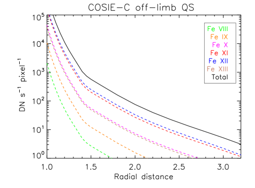
Figure 7.— The estimated total count rates (per pixel) in the COSIE-C broad-band, as a function of the radial distance, for the quiet Sun, using the UVCS model. The total rates are shown, as well as those produced by the main ions.

Figure 8.— COSIE-C predicted spectrum at 3 $\rm R_{\odot}$.

The resulting total count rates expected for off-limb quiet Sun observations are shown in Figure 7. As expected, the signal is so high close to the limb that a filter will have to be used, together with very short exposure times, which will allow unprecedented high-cadence observations, useful to study fast dynamics and waves. Very high cadence of tens of seconds could in principle be achieved even at 3  $\rm R_{\odot}$ in bright streamers and transient solar wind structures, depending on the stray light levels (see discussion in Section 5).

Figure 7 also shows a breakdown of the contributions from the main ions. As expected, the dominating contributions are from Fe xi, and Fe xii, i.e. ions that are formed at similar temperatures. In other words, although COSIE-C is a broad-band instrument, it is not as multithermal as most of the SDO AIA bands, although extra contributions from much cooler (O v) or hotter (Ca xvii and Fe xxiv) lines could occasionally be present. As shown e.g. in Del Zanna et al. (2011) and Del Zanna (2013b), having a very multithermal band often complicates the analysis of solar observations.

4. QS Hinode EIS off-limb

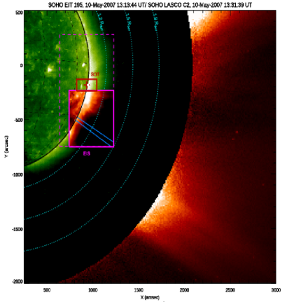
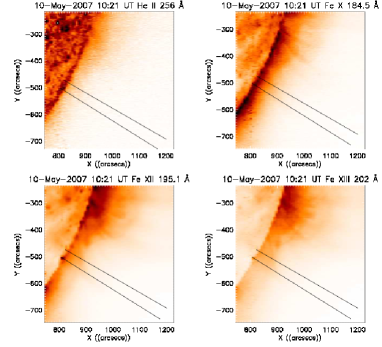
Figure 9.— From top to bottom: 1) a SOHO EIT 195 Å image on 2007 May 10, with the Hinode EIS field of view (full possible, pink dashed rectangle; observed, full pink lines) and the EIS Fe xii 195.1 Å monochromatic image. The blue lines indicate the radial sector used for the averaging (see text). The SOHO LASCO C2 image is superimposed, showing that the selected radial sector is in a streamer. 2) Monochromatic images (negative) in a few spectral lines, with the radial sector indicated. 3) the observed radial variation of the radiances of the main coronal lines. The full line is the estimated radiance in the Fe xiii 202.0 Å line, based on the modelling of the 1996 solar minimum quiet Sun streamer.

As Hinode pointing outside the solar limb is normally not allowed, almost all the off-limb quiet Sun EIS observations are restricted to about 1.2  $\rm R_{\odot}$. There are only a few observations to greater distances, but they were in polar coronal holes, where the edge of the EIS slit reached about 1.4  $\rm R_{\odot}$. One of us (GDZ) designed an engineering EIS ’study’ to extract spectra from the bottom half of the long EIS slit, to reach greater distances. A week-long campaign (Hinode HOP 7) was coordinated to obtain simultaneous SOHO/Hinode/TRACE/STEREO observations during the SOHO-Ulysses quadrature in May 2007. EIS observations were obtained during May 7–10, as outlined in Del Zanna et al. (2009). The Sun was very quiet, with the exception of an active region, which was at the west limb around May 7, as shown in Fig. 9(top). The Figure also shows the field of view covered by EIS. The lower part of the EIS field of view reached the significant distance of 1.5  $\rm R_{\odot}$. On May 10, the main part of the active region was behind the limb. We have selected the observation which started on that day at 10:21 UT. The EIS 2″ slit was moved with 8″ jumps, to cover about 500″ in the E-W direction. A long exposure of 60s was chosen. As far as we are aware, this is the only EIS observation of the quiet Sun up to such large distances.

The EIS data have been processed with custom-written software written by GDZ and radiometrically calibrated using the Del Zanna (2013a) analysis (see below). Monochromatic images in a few lines are shown in Fig. 9(middle). The He ii 256 Å line was deblended from the contribution of a strong coronal Si x using the 261 Å line. Some emission associated with the active region is still visible in the north portion of the EIS field of view. Aside from a region up to 1.1  $\rm R_{\odot}$, where some structures are present, the outer corona is featureless, although it bears some differences with the quiet Sun observations during the 1996 solar minimum presented above.

An off-limb region about 5^o wide, along the radial direction indicated in Fig. 9 was chosen, to obtain averaged intensities as a function of the radial distance, which are shown in Fig. 9 (bottom). They were obtained by first averaging about 15-20 EIS pixels, then obtain the averaged spectra and then the integrated intensities. The uncertainties include the Poisson noise associated with the number of detected photons in the line and nearby pseudo-continuum, plus the read-out noise.

Only a few of the strongest EIS lines had good signal at 1.5  $\rm R_{\odot}$: Fe xi 188.2 Å (a self-blend), the Fe xii 192.4 Å and 195.1 Å (a self-blend), and the Fe xiii 202.0 Å. The Fe x 184.5 Å line was barely visible. Figure 10 shows averaged spectra at the larger distance, 1.5  $\rm R_{\odot}$. Note that the apparent continuum around 10 DN is actually the detector bias, which was not subtracted. All the other lines had strong signal only up to about 1.2–1.3  $\rm R_{\odot}$.

Figure 10.— Hinode EIS spectra of the stronger lines at 1.5  $\rm R_{\odot}$.

The behavior of the cooler lines, discussed below when we consider stray light, indicates negligible stray light for this observation, hence confirming that the signal in the coronal lines is real, and not scattered light from the disk. Fig. 9 (bottom) shows with a full line the radiances of the Fe xiii 202.0 Å, as estimated using the 1996 UVCS streamer observation. This is significantly lower than the observed Fe xiii 202.0 Å radiance.

Figure 11.— Averaged densities and temperatures obtained from EIS.

We have explored the possible reasons for this difference, by measuring the densities and temperatures from the EIS lines, which are shown in Figure 11. Measuring densities is very difficult because of the low signal in the density-sensitive lines. We obtain relatively good agreement between two of the main density ratios available to EIS at 1–2 MK, from Fe xii and Si x (for a discussion of available ratios see Del Zanna (2012)) using the Del Zanna (2013a) radiometric calibration, and not the ground calibration, where the Fe xii densities are unreasonably low. The averaged electron densities of this region/streamer are slightly higher than those we assumed in our model, which explains some of the differences.

Some further differences are probably related to the temperature of the plasma. Figure 11 (bottom) shows that we obtain an excellent agreement in the ionization temperatures from ratios involving Fe x, Fe xi, and Fe xii. It is remarkable that these also indicate a temperature (averaged along the line of sight) nearly constant with radial distance, although slightly lower, log $T$ [K]=6.12 instead of log $T$ [K]=6.15. Note that this result is surely independent from any stray light. The absolute value depends however on the accuracy of the ionization and recombination rates, which are constantly under revision. On the other hand, the ratio involving the hotter Fe xiii indicates the presence of a slightly hotter component. This was to be expected, considering the presence of the active region not far away.

5. Stray light

Stray light, i.e. the light scattered within an instrument, is an important quantity to be estimated for any instrument. Such estimates are notoriously difficult to obtain, and have not received as much attention in the literature as they should have. Stray light varies significantly with each instrument (as it depends e.g. on the micro-roughness of the optics, the filters, the optical paths), but also depends on the illumination, i.e. on where one is observing.

Out-of-field stray light is often estimated by off-pointing the spacecraft, while in-field stray light is often estimated looking at the on-disk signal when part of the Sun is occulted by a planet, such as Venus or the Moon. The signals are often close to the noise levels, and it is always hard to assess for the real presence of a coronal signal.

Several EUV imagers have shown non-negligible stray light, in the wings of the PSF, for example SoHO EIT (Auchère et al., 2001), STEREO EUVI (see, e.g. Shearer et al., 2012) and SWAP/PROBA2 (see, e.g. Halain et al., 2013; Goryaev et al., 2014). Earlier instruments had a lot more stray light, while the performance of more recent ones has improved significantly. One earlier instrument with an excellent performance was the 1998 SwRI/LASP Multiple XUV Imager (MXUVI), which flew on a sounding rocket for the SoHO EIT calibration (Auchère et al., 2001). The instrument had a highly-polished (0.5 Å rms) single mirror with a multilayer in the 171 Å band, a front filter, a light trap and baffles to reduce scattered light. The detected signal was about 1% the disk intensity at 1.5  $\rm R_{\odot}$, and about $3\times 10^{-3}$ at 2  $\rm R_{\odot}$ (cf. Fig. 8 in Auchère et al., 2001). Considering that the strong coronal Fe ix 171 Å line would always emit some signal in this band even at such distances, one could argue that the level of stray light was for sure less than the detected signal.

Another instrument with excellent performance was the Normal Incidence X-ray Telescope (NIXT), which was developed at SAO and used multilayers. This instrument paved the way for all the subsequent EUV multilayers flown in all the solar missions. During a NIXT rocket flight on 1991 July 11, a knife-edge test using the edge of the Moon was carried out. The results indicated that the level of scattered light was less than $5\times 10^{-4}$ the disk intensity (Spiller et al., 1994).

The COSIE optical setup is unique, and a thorough assessment of the stray light will only be possible once all the components are fabricated and measured. However, as all the components have significant heritage from other missions, we can provide some comments on what would be expected, mostly based on the performances of SDO/AIA and Hinode/EIS.

Two of the main sources of stray light we expect are the scattering of the mesh supporting the two aluminum filters, and the scattering of the optics. The main mirror and multilayer will have performances improved over the SDO AIA ones, and similar to those of the Hi-C instrument. The mesh will be a significant improvement. The AIA telescopes have two filters (one internal and one external) and two mirrors, polished to a micro roughness of about 1–2.5 Å rms (Soufli et al., 2007), and both coated with multilayers (Lemen et al., 2012). As described in the on-line report on the AIA PSF (Grigis & the AIA team, 2012), by far the single biggest factor contributing to scattered light in AIA is the diffraction caused by the support mesh of the filters. That can be quantified and deconvolved. There remains a residual from imperfect removal of that diffracted component, and the main way to reduce it is to use a much wider mesh. This has been implemented for the Hi-C rocket flights (Kobayashi et al., 2014) and will be implemented for COSIE. The diffracted component due to the mesh goes down from 20% in all previous instruments, including EIS and AIA, to about 2%, hence will be much reduced for COSIE. Observations of the lunar limb during partial eclipses were used to get the scattering in each of the AIA channels. The scattering in the EUV was estimated to be about 10${}^{{}^{-}5}$ per surface, i.e. negligible. The only other source of scattering we are aware of is some very wide-angle scattering produced by multilayers, which has been measured in one instance (see, e.g. Martínez-Galarce et al., 2010).

González et al. (2016) estimated the AIA PSF using both lunar and Venus occultations, however the validity of using Venus has been questioned (Afshari et al., 2016). Poduval et al. (2013) also used a lunar occultation to provide an estimate of the AIA PSF. Typically, both the full-Sun deconvolution method (Grigis & the AIA team, 2012), and that one suggested by Poduval et al. (2013) produce similar results, with changes in the on-disk intensities by 10–20%, but mostly negligible off-limb, with a large amount of noise.

One could in principle estimate an upper limit on stray light directly from off-limb observations. However, the coronal EUV bands in AIA cannot be used as the corona would produce some signal. The He II 304 Å line has a significant coronal emission (Andretta et al., 2012) and most likely a resonantly scattered component (Delaboudinière, 1999), so it cannot be used. The only band perhaps usable is the 131 Å, as this band is dominated by cool emission, mostly from Fe viii with some contributions from Ne vi and O vi (Del Zanna et al., 2011). The signal for this band quickly reaches near off-limb (i.e. even in a region where some solar signal should be present) a noise level (i.e. 1–2 DN per pixel) at about 8% the average on-disk signal, with the standard 3s exposures for this band. There are also a few off-point AIA observations which in principle could be used. We analyzed those of 2013 Nov 13 and 28, but did not find them suitable to assess stray light, as standard exposures were used.

There are calibration data with longer exposures. Among the longest exposures (32s), we analyzed those taken on 2011 Aug 17. Even with these long exposures the average signal on-disk is only about 200 DN (see Figure 12), so if there was say a 2% stray light at 1.5  $\rm R_{\odot}$, one should see a flattening of the off-limb signal towards about 4 DN. This is not observed, as shown in Figure 12, although it also cannot be ruled out, given the low signal and noise. To obtain the points in the figure, we have averaged four consecutive exposures (using level 1 data) over a radial sector in a quiet Sun SW region. Solar structures are clearly visible out to 1.2–1.3  $\rm R_{\odot}$, so some solar contribution out to 1.5  $\rm R_{\odot}$ is still possible. The optical layout of the AIA telescopes is such that the FOV is annular, i.e. in the images there are four corners, above 1.54  $\rm R_{\odot}$, that are not illuminated. They can be used to assess the level or read-out noise in the level 1 data (which have been corrected for the dark frames and flat-field). We found an average DN=0.7 with a standard deviation of 2.5 DN/pixel. The ’error bars’ in Figure 12 are the standard deviation of the ensemble of points averaged at each radial distance, plus the 2.5 DN/pixel noise level, to provide an estimate on the level of noise in the data.

Figure 12.— The observed radial fall-off in the AIA 131 Å band.

The stray light in Hinode EIS has not been studied in depth. Lunar occultations were used by Ugarte (2010) to suggest a 2% level of stray light for the instrument. This was obtained from the residual signal in the 195 Å line, once dark frames were removed. A broad distribution of DN values, centered at 5.2 and 5.8$\pm$4.1 was found, depending on which dark frame was used. Note that the dark frames are highly variable in time and spatially, and have large DN values, of about 500. The same procedure was applied to the strongest line in the long-wavelength channel at 256 Å, to find distributions centered at -1.2$\pm$3.6 and 0.8$\pm$3.7 DN. It is unclear why the two results are so different, and if a 2% stray light is real. More importantly, it is not clear how such on-disk observations could be used to estimate the actual stray light in far off-limb observations.

Hahn et al. (2012) used a model to estimate the near off-limb (up to 1.3  $\rm R_{\odot}$) signal in coronal holes one should expect in the 256 Å line and found excellent agreement with the observed fall-off (cf. their Fig. 2) which was well below the 2% level, suggesting negligible stray light off-limb.

Figure 13.— The observed radial fall-off in the cooler EIS lines (cf. bottom of Figure 9). The two dashed lines indicate 2% and 0.5% levels from the on-disk values.

Considering the off-limb observations we have presented in this paper, as they are rather unique (using the bottom part of the EIS slit), there is no available information on the instrument performance. However, we can also assess for possible levels of stray light by measuring the off-limb behavior in the cooler lines, where negligible signal from the outer corona would normally be expected. The strongest line is at 256.3 Å, a complex blend of He ii and several coronal lines (see section 3.3. in Del Zanna et al., 2011b). We could only deblend the Si x contribution using a branching ratio with the 261 Å line, but the signal was such this could only be feasible up to 1.2  $\rm R_{\odot}$. We therefore consider this line not suitable for off-limb measurements of the stray light. We have therefore considered all the other strongest cool transition-region lines, mostly from Fe viii and Si vii, recorded for this observation. There is some signal in these lines at various distances up to 1.4  $\rm R_{\odot}$, as shown in Fig. 13. The 2% level from the on-disk intensities is shown with the upper dashed curve. It is clear that in this case a 2% level of stray light at 1.5  $\rm R_{\odot}$ is an overestimate. Considering that some of the measured signal could actually be real, a more conservative $5\times 10^{-3}$ (lower dashed curve) should be used.

In conclusions, on the basis of off-limb AIA and EIS observations, a level of stray light between $5\times 10^{-3}$ and 2% at 1.5  $\rm R_{\odot}$ is possible. Regarding the amount of stray light that would be acceptable by COSIE-C, we note that we would require that the coronal emission at say 3  $\rm R_{\odot}$  should be greater than the fluctuations in the scattered disk emission $SD$. Assuming Poisson noise on the number of detected photons $D$, we therefore require that $D(3~{}\mbox{\,$\rm R_{\odot}$})>\sqrt{SD(3~{}\mbox{\,$\rm R_{\odot}$})}$. On the basis of Figure 7 and Eq. 1, at around 3  $\rm R_{\odot}$  we expect to detect about 2 photons/pixel/s, i.e. 120 photons/pixel for a 60s exposure time. The disk signal is about 10⁵ photons/pixel/s, so we would require the stray light to be less than $3\times 10^{-3}$ the disk radiation, at 3  $\rm R_{\odot}$. This appears achievable, considering the above discussion. We would in fact expect the stray light to decrease with radial distance from the Sun, and if we assume that this decrease follows the observed decrease in the MXUVI signal, a 1% level at 1.5  $\rm R_{\odot}$  would already provide the required stray light at 2  $\rm R_{\odot}$. A 2% stray light at 1.5  $\rm R_{\odot}$ would be $6\times 10^{-3}$ at 2  $\rm R_{\odot}$ and most likely less than the requirement at 3  $\rm R_{\odot}$. If stray light will turn out to be higher than $3\times 10^{-3}$ at 3  $\rm R_{\odot}$, one would have to reduce the spatial resolution (i.e. binning) and/or increase the exposure time (60s) to detect the coronal signal in quiescent streamers.

6. Some estimates for other regions

Aside from quiet Sun streamers, perhaps the most important science targets for COSIE-C will be active region streamers. To estimate what kind of signal might be expected, we have extended the search on UVCS observations during the first year of operations, to try and find streamers above active regions. We found only one useful observations on 1996 June 1, also shown in Figure 2. This is because the other active region observations had very little signal, either because of too short exposure times and/or narrow slits, or only observed below 2  $\rm R_{\odot}$. The selected streamer was above two active regions, a compact small one and a diffuse one. The streamer is not as bright as streamers observed later on when the solar activity increased, but provides an idea of how the signal increases above an AR. The radiances of the lines are shown in Figures 3,4,5. The increases are significant, especially those of the hotter Si xii 521 Å line, which is brighter by over an order of magnitude closer to the limb, as one would expect. However, the radiances at 3.1  $\rm R_{\odot}$  are less than a factor of two higher than those of the quiet Sun streamers. We therefore expect similar increases in the COSIE-C signal, compared to the quiet Sun estimates. With high solar activity, the COSIE-C signal would increase much more.

As we have mentioned, CMEs are also a primary target for COSIE-C. Many CMEs will also be bright in the COSIE passband. We are developing models to study the COSIE signal, but a full discussion is beyond the scope of the present paper, as it is quite a complex issue.

What we can say, on the basis of previous observations, is that the fluxes will vary enormously from event to event, and different structures (cooler and hotter) will be visible by COSIE. For example, UVCS spectra of CME cores generally show plasma at transition region temperatures, and COSIE images are likely to be dominated by the O V 193 Å multiplet (see, e.g. Ciaravella et al., 2000). Higher temperature emission is seen in AIA 195, 211 and 335 Å images (cf. Ma et al., 2011) and UVCS spectra show CME-driven shock waves (Raymond et al., 2000). Flare-CME current sheets are seen in high temperature lines such as [Fe XVIII] and Fe XXIV (see, e.g. Bemporad et al., 2006; Warren et al., 2018), and the leading edges of CMEs appear in several AIA bands (see, e.g. Kozarev et al., 2011) and in coronal emission lines observed with UVCS, so they should be easily detectable with COSIE’s higher sensitivity. For example, Giordano et al. (2013) presented an UVCS catalog of CME events from 1996 to 2005, where a number of coronal lines as the Si XII doublet were clearly observed. We can therefore predict that COSIE would easily observe such events.

Finally, we note that coronal holes are not a primary scientific target for the COSIE mission. Their densities in the outer corona are significantly lower than those of the quiet Sun streamers. For example, Abbo et al. (2010) measured a density of 1.1$\times$10⁶ cm^-3 at 2.2  $\rm R_{\odot}$ in a streamer, while they found a value of 6.5$\times$10⁵ cm^-3 in a region that would generally be considered part of the coronal hole (their region 4, though it might be a projection of another streamer). Also, coronal holes have lower temperatures, so the EUV signal would be significantly lower than that for the QS streamers, probably by a factor of 10–100, in reasonable agreement with the model of Shen et al. (2017). If stray light were not a factor, increasing exposure times and spatial binning would make coronal holes observable with COSIE-C.

7. Conclusions

An EUV coronagraph such as COSIE has a great potential for novel observations of the outer corona, especially between 1.5 and 3  $\rm R_{\odot}$, where many fundamental processes affecting the generation of the solar wind but also the evolution of structures in the low corona are taking place. This region is still nearly unexplored.

We have a long heritage of coronagraph observations at visible wavelengths, which has notorious difficulties in reducing the disk light and in observing the corona close to the Sun. This is not an issue for COSIE in its coronagraph mode, which will allow, with the use of a filter, both on-disk and off-limb observations out to 3.3  $\rm R_{\odot}$.

It might seem surprising, but we have shown here that significant signal in lines collisionally excited is still present at least until 3.1  $\rm R_{\odot}$, i.e. 2  $\rm R_{\odot}$ above the photosphere. The few SOHO UVCS observations we were able to find clearly show this. We are confident about these results. We have also clearly shown that the same EUV lines of the COSIE instrument have been easily observed by Hinode EIS in a relatively quiet period in 2007 out to 1.5  $\rm R_{\odot}$.

The main conclusion of the present study is that, on the basis of current baseline designs, COSIE-C exposures of the order of tens of seconds will be sufficient to observe quiescent streamers at 3  $\rm R_{\odot}$, if stray light issues will turn to be negligible. This is unprecedented (except for images during eclipses), when considered in combination with a spatial resolution of 3″.

We have briefly discussed stray light issues. As there are discrepancies in assessing the stray light in current instruments, and stray light very much depends on the actual optical layout and components (e.g. filters), we defer an assessment to a future study, noting that our current knowledge on the basis of AIA and EIS performances indicates that COSIE-C, with improved filters and micro-roughness of the main optical surface, should have a negligible stray light.

A secondary main conclusion is that variations in the outer corona of the electron densities and temperatures obtained from models fail to explain the observations. It is surprising, but the ionization temperature of the outer corona seems to be relatively constant out to 3.1  $\rm R_{\odot}$, at least on the basis of the few observations from UVCS and EIS presented here. That the temperature is nearly isothermal and constant with height was known from previous SOHO CDS and Hinode EIS measurements, but only up to 1.2  $\rm R_{\odot}$.

The relative radiances between the coronal lines and the H i Lyman $\beta$ observed by UVCS indicate photospheric abundances in the quiescent 1996 streamers, using the present model. The Lyman $\beta$ line is mostly collisional at 1.4  $\rm R_{\odot}$, so this result is largely independent on the photoexcitation and the density distribution of the plasma. It is interesting to note that this result is in agreement with a recent revision by Del Zanna & DeLuca (2018) of SOHO SUMER observations near the solar limb during the same period.

There are however several complexities related to the interpretation and modelling of the UVCS Lyman and O vi lines that are significantly photo-excited, and which could also affect these elemental abundance measurements at larger distances, so these abundance measurements will need to be confirmed.

References

- Abbo et al. (2010) Abbo, L., Antonucci, E., Mikić, Z., Linker, J. A., Riley, P., & Lionello, R. 2010, Advances in Space Research, 46, 1400
- Abbo et al. (2016) Abbo, L., et al. 2016, Space Sci. Rev., 201, 55
- Afshari et al. (2016) Afshari, M., Peres, G., Jibben, P. R., Petralia, A., Reale, F., & Weber, M. 2016, AJ, 152, 107
- Andretta et al. (2012) Andretta, V., Telloni, D., & Del Zanna, G. 2012, Sol. Phys., 279, 53
- Antiochos et al. (2011) Antiochos, S. K., Mikić, Z., Titov, V. S., Lionello, R., & Linker, J. A. 2011, ApJ, 731, 112
- Antonucci et al. (2005) Antonucci, E., Abbo, L., & Dodero, M. A. 2005, A&A, 435, 699
- Antonucci et al. (2006) Antonucci, E., Abbo, L., & Telloni, D. 2006, ApJ, 643, 1239
- Asplund et al. (2009) Asplund, M., Grevesse, N., Sauval, A. J., & Scott, P. 2009, ARA&A, 47, 481
- Auchère et al. (2001) Auchère, F., Hassler, D. M., Slater, D. C., & Woods, T. N. 2001, Sol. Phys., 202, 269
- Bemporad et al. (2006) Bemporad, A., Poletto, G., Suess, S. T., Ko, Y.-K., Schwadron, N. A., Elliott, H. A., & Raymond, J. C. 2006, ApJ, 638, 1110
- Boerner et al. (2012) Boerner, P., et al. 2012, Sol. Phys., 275, 41
- Bradshaw et al. (2011) Bradshaw, S. J., Aulanier, G., & Del Zanna, G. 2011, ApJ, 743, 66
- Brueckner et al. (1995) Brueckner, G. E., et al. 1995, Sol. Phys., 162, 357
- Ciaravella et al. (2000) Ciaravella, A., et al. 2000, ApJ, 529, 575
- Cranmer et al. (2007) Cranmer, S. R., van Ballegooijen, A. A., & Edgar, R. J. 2007, ApJS, 171, 520
- Del Zanna (1999) Del Zanna, G. 1999, Ph.D. thesis, Univ. of Central Lancashire, UK
- Del Zanna (2008) Del Zanna, G. 2008, A&A, 481, L49
- Del Zanna (2012) Del Zanna, G. 2012, A&A, 537, A38
- Del Zanna (2013a) Del Zanna, G. 2013a, A&A, 555, A47
- Del Zanna (2013b) Del Zanna, G. 2013b, A&A, 558, A73
- Del Zanna & Andretta (2015) Del Zanna, G., & Andretta, V. 2015, A&A, 584, A29
- Del Zanna et al. (2009) Del Zanna, G., et al. 2009, in Astronomical Society of the Pacific Conference Series, Vol. 415, The Second Hinode Science Meeting: Beyond Discovery-Toward Understanding, ed. B. Lites, M. Cheung, T. Magara, J. Mariska, & K. Reeves, 315
- Del Zanna et al. (2011a) Del Zanna, G., Aulanier, G., Klein, K.-L., & Török, T. 2011a, A&A, 526, A137
- Del Zanna & Bromage (1999) Del Zanna, G., & Bromage, B. J. I. 1999, J. Geophys. Res., 104, 9753
- Del Zanna & DeLuca (2018) Del Zanna, G., & DeLuca, E. E. 2018, ApJ, 852, 52
- Del Zanna et al. (2015) Del Zanna, G., Dere, K. P., Young, P. R., Landi, E., & Mason, H. E. 2015, A&A, 582, A56
- Del Zanna & Mason (2018) Del Zanna, G., & Mason, H. E. 2018, Living Reviews in Solar Physics, in press
- Del Zanna et al. (2011b) Del Zanna, G., Mitra-Kraev, U., Bradshaw, S. J., Mason, H. E., & Asai, A. 2011b, A&A, 526, A1
- Del Zanna et al. (2011) Del Zanna, G., O’Dwyer, B., & Mason, H. E. 2011, A&A, 535, A46
- Del Zanna et al. (2012a) Del Zanna, G., Storey, P. J., Badnell, N. R., & Mason, H. E. 2012a, A&A, 541, A90
- Del Zanna et al. (2012b) Del Zanna, G., Storey, P. J., Badnell, N. R., & Mason, H. E. 2012b, A&A, 543, A139
- Del Zanna et al. (2014) Del Zanna, G., Storey, P. J., Badnell, N. R., & Mason, H. E. 2014, A&A, 565, A77
- Delaboudinière (1999) Delaboudinière, J. P. 1999, Sol. Phys., 188, 259
- Dere et al. (1997) Dere, K. P., Landi, E., Mason, H. E., Monsignori Fossi, B. C., & Young, P. R. 1997, A&AS, 125, 149
- Doschek et al. (2008) Doschek, G. A., Warren, H. P., Mariska, J. T., Muglach, K., Culhane, J. L., Hara, H., & Watanabe, T. 2008, ApJ, 686, 1362
- Feldman et al. (1998) Feldman, U., Schühle, U., Widing, K. G., & Laming, J. M. 1998, ApJ, 505, 999
- Fisk (2003) Fisk, L. A. 2003, Journal of Geophysical Research (Space Physics), 108, 1157
- Fludra et al. (1999) Fludra, A., Del Zanna, G., Alexander, D., & Bromage, B. J. I. 1999, J. Geophys. Res., 104, 9709
- Frazin et al. (2003) Frazin, R. A., Cranmer, S. R., & Kohl, J. L. 2003, ApJ, 597, 1145
- Gibson et al. (1999) Gibson, S. E., Fludra, A., Bagenal, F., Biesecker, D., del Zanna, G., & Bromage, B. 1999, J. Geophys. Res., 104, 9691
- Giordano et al. (2013) Giordano, S., Ciaravella, A., Raymond, J. C., Ko, Y.-K., & Suleiman, R. 2013, Journal of Geophysical Research (Space Physics), 118, 967
- González et al. (2016) González, A., Delouille, V., & Jacques, L. 2016, Journal of Space Weather and Space Climate, 6, A1
- Goryaev et al. (2014) Goryaev, F., Slemzin, V., Vainshtein, L., & Williams, D. R. 2014, ApJ, 781, 100
- Grigis & the AIA team (2012) Grigis, P., & the AIA team., AIA PSF report
- Habbal et al. (2011) Habbal, S. R., et al. 2011, ApJ, 734, 120
- Hahn et al. (2012) Hahn, M., Landi, E., & Savin, D. W. 2012, ApJ, 753, 36
- Halain et al. (2013) Halain, J.-P., et al. 2013, Sol. Phys., 286, 67
- Harra et al. (2008) Harra, L. K., Sakao, T., Mandrini, C. H., Hara, H., Imada, S., Young, P. R., van Driel-Gesztelyi, L., & Baker, D. 2008, ApJ, 676, L147
- Kobayashi et al. (2014) Kobayashi, K., et al. 2014, Sol. Phys., 289, 4393
- Kohl et al. (1995) Kohl, J. L., et al. 1995, Sol. Phys., 162, 313
- Kozarev et al. (2011) Kozarev, K. A., Korreck, K. E., Lobzin, V. V., Weber, M. A., & Schwadron, N. A. 2011, ApJ, 733, L25
- Laming (2015) Laming, J. M. 2015, Living Reviews in Solar Physics, 12
- Landi & Feldman (2003) Landi, E., & Feldman, U. 2003, ApJ, 592, 607
- Lemen et al. (2012) Lemen, J. R., et al. 2012, Sol. Phys., 275, 17
- Ma et al. (2011) Ma, S., Raymond, J. C., Golub, L., Lin, J., Chen, H., Grigis, P., Testa, P., & Long, D. 2011, ApJ, 738, 160
- Martínez-Galarce et al. (2010) Martínez-Galarce, D., Harvey, J., Bruner, M., Lemen, J., Gullikson, E., Soufli, R., Prast, E., & Khatri, S. 2010, in Proc. SPIE, Vol. 7732, Space Telescopes and Instrumentation 2010: Ultraviolet to Gamma Ray, 773237
- Mierla et al. (2008) Mierla, M., Schwenn, R., Teriaca, L., Stenborg, G., & Podlipnik, B. 2008, A&A, 480, 509
- Mikić et al. (2007) Mikić, Z., Linker, J. A., Lionello, R., Riley, P., & Titov, V. 2007, in Astronomical Society of the Pacific Conference Series, Vol. 370, Solar and Stellar Physics Through Eclipses, ed. O. Demircan, S. O. Selam, & B. Albayrak, 299
- Noci & Gavryuseva (2007) Noci, G., & Gavryuseva, E. 2007, ApJ, 658, L63
- Noci et al. (1987) Noci, G., Kohl, J. L., & Withbroe, G. L. 1987, ApJ, 315, 706
- Parenti et al. (2000) Parenti, S., Bromage, B. J. I., Poletto, G., Noci, G., Raymond, J. C., & Bromage, G. E. 2000, A&A, 363, 800
- Poduval et al. (2013) Poduval, B., DeForest, C. E., Schmelz, J. T., & Pathak, S. 2013, ApJ, 765, 144
- Raymond et al. (1997) Raymond, J. C., et al. 1997, Sol. Phys., 175, 645
- Raymond et al. (2000) Raymond, J. C., et al. 2000, Geophys. Res. Lett., 27, 1439
- Schrijver & Higgins (2015) Schrijver, C. J., & Higgins, P. A. 2015, Sol. Phys., 290, 2943
- Shearer et al. (2012) Shearer, P., Frazin, R. A., Hero, A. O., III, & Gilbert, A. C. 2012, ApJ, 749, L8
- Shen et al. (2017) Shen, C., Raymond, J. C., Mikić, Z., Linker, J. A., Reeves, K. K., & Murphy, N. A. 2017, ApJ, 850, 26
- Soufli et al. (2007) Soufli, R., Baker, S. L., Windt, D. L., Gullikson, E. M., Robinson, J. C., Podgorski, W. A., & Golub, L. 2007, Appl. Opt., 46, 3156
- Spadaro et al. (2007) Spadaro, D., Susino, R., Ventura, R., Vourlidas, A., & Landi, E. 2007, A&A, 475, 707
- Spiller et al. (1994) Spiller, E., Barbee, T. W., Golub, L., Kalata, K., Nystrom, G. U., & Viola, A. 1994, in Proc. SPIE, Vol. 2011, Multilayer and Grazing Incidence X-Ray/EUV Optics II, ed. R. B. Hoover & A. B. Walker, 391
- Strachan et al. (2002) Strachan, L., Suleiman, R., Panasyuk, A. V., Biesecker, D. A., & Kohl, J. L. 2002, ApJ, 571, 1008
- Temmer et al. (2017) Temmer, M., Thalmann, J. K., Dissauer, K., Veronig, A. M., Tschernitz, J., Hinterreiter, J., & Rodriguez, L. 2017, Sol. Phys., 292, 93
- Ugarte (2010) Ugarte, I., EIS software note No. 12
- Uzzo et al. (2003) Uzzo, M., Ko, Y.-K., Raymond, J. C., Wurz, P., & Ipavich, F. M. 2003, ApJ, 585, 1062
- Uzzo et al. (2006) Uzzo, M., Strachan, L., Vourlidas, A., Ko, Y.-K., & Raymond, J. C. 2006, ApJ, 645, 720
- Vásquez et al. (2003) Vásquez, A. M., van Ballegooijen, A. A., & Raymond, J. C. 2003, ApJ, 598, 1361
- Warren et al. (2018) Warren, H. P., Brooks, D. H., Ugarte-Urra, I., Reep, J. W., Crump, N. A., & Doschek, G. A. 2018, ApJ, 854, 122
- Weberg et al. (2015) Weberg, M. J., Lepri, S. T., & Zurbuchen, T. H. 2015, ApJ, 801, 99
- Weberg et al. (2012) Weberg, M. J., Zurbuchen, T. H., & Lepri, S. T. 2012, ApJ, 760, 30
- Wilhelm et al. (1998) Wilhelm, K., et al. 1998, A&A, 334, 685
- Young et al. (2003) Young, P. R., Del Zanna, G., Landi, E., Dere, K. P., Mason, H. E., & Landini, M. 2003, ApJS, 144, 135
- Zhang & Dere (2006) Zhang, J., & Dere, K. P. 2006, ApJ, 649, 1100