Metrics for Signal Temporal Logic Formulae

Abstract

Signal Temporal Logic (STL) is a formal language for describing a broad range of real-valued, temporal properties in cyber-physical systems. While there has been extensive research on verification and control synthesis from STL requirements, there is no formal framework for comparing two STL formulae. In this paper, we show that under mild assumptions, STL formulae admit a metric space. We propose two metrics over this space based on i) the Pompeiu-Hausdorff distance and ii) the symmetric difference measure, and present algorithms to compute them. Alongside illustrative examples, we present applications of these metrics for two fundamental problems: a) design quality measures: to compare all the temporal behaviors of a designed system, such as a synthetic genetic circuit, with the “desired” specification, and b) loss functions: to quantify errors in Temporal Logic Inference (TLI) as a first step to establish formal performance guarantees of TLI algorithms.

I Introduction

Temporal logics [1] are increasingly used for describing specifications in cyber-physical systems such as robotics [2], synthetic biology [3], and transportation  [4]. Variants of temporal logics, such as Computation Tree Logic (CTL) [5], Linear Temporal Logic (LTL) [6], or Signal Temporal Logic (STL) [7], can naturally describe a wide range of temporal system properties such as safety (never visit a “bad” state), liveness (eventually visit a “good” state), sequentiality, and their arbitrarily elaborate combinations.

Using model checking [1] techniques, signals or traces can be checked to determine whether or not they satisfy a specification. For STL in particular, the degree of satisfaction or robustness is a quantitative measure to characterize how far a signal is from satisfaction [8, 9, 10] of an STL formula. There is currently, however, no formal way to directly compare specifications against each other. Previous related approaches in planning and control have looked into specification relaxation, where the goal is to minimally enlarge the specification language to include a satisfying control policy for the system model. Various specification relaxations have been defined including minimum violation [11, 12, 13] for self-driving cars, temporal relaxation of deadlines [14], minimum revision of Büchi automata [15], and diagnosis and repair in reactive synthesis [16]. While language inclusion and equivalence problems are of paramount importance in computer science and control theory, they are only qualitative measures while we are interested in quantitative metrics.

This paper presents two metrics that can be used to compute the distance between two STL specifications. Under mild assumptions, we propose the metrics based on the languages of STL formulae. We propose two distance functions. The first is based on the Pompeiu-Hausdorff (PH) distance [17], which captures how much the language of one formula must be enlarged to include the other, and the second is based on the symmetric difference (SD) [18], which characterizes how much overlap there is between the two formulae. The theoretical contributions of this paper are:

1. formalization of STL formulae metrics based on the PH and the SD distances, and

2. methods for computing the PH using mixed-integer linear programming (MILP), and the SD using a recursive algorithm based on the area of satisfaction.

We discuss the comparison of the two metrics in detail and provide examples that highlight their differences.

This paper additionally presents applications of the proposed metrics to a behavioral synthesis problem and to the evaluation of temporal logic inference (TLI) [19, 20, 21, 22, 23] methods. In the first case, we are interested in generating designs that exhibit desired behaviors specified in STL. For example, we study synthetic genetic circuits. Possible circuit designs are constructed and measured in laboratory experiments, and the resulting traces are abstracted into STL specifications using TLI. These formulae are compared quantitatively against the desired design specification using the proposed metrics. The second setup considers the fundamental problem of evaluating TLI methods themselves. Under the assumption that data used for inference can be characterized by ground truth STL formulae, we ask the question of how well the TLI algorithms perform. As opposed to empirical evaluation used in previous work, we propose to use our metrics as loss functions as the first step in establishing theoretical foundations for TLI. The related contributions are:

1. a design quality measure for evaluating proposed implementations against an STL specification, and

2. a loss function to quantify errors in TLI as a first step in establishing formal performance guarantees of TLI algorithms.

II Preliminaries

Notation

Let $\mathbb{R},\mathbb{R}_{\geq 0}$, $\mathbb{N}$ denote the set of real, non-negative real, and natural numbers, respectively. We use $|r|$ to denote the absolute value of $r\in\mathbb{R}$. Given $x\in\mathbb{R}^{n}$, $\left\|x\right\|_{\infty}:=\max_{i\in\{1,\cdots,n\}}|x^{i}|$ - where $x^{i}$ is the $i$’th component of $x$ - is its infinity-norm. A scalar-valued function $f:\mathbb{R}^{n}\rightarrow\mathbb{R}$ is rectangular if for some $i\in\{1,\cdots,n\}$, $f(x)=x^{i}$. A metric space is an ordered pair $(\mathcal{M},d)$, where $\mathcal{M}$ is a set and $d:\mathcal{M}\times\mathcal{M}\rightarrow\mathbb{R}_{\geq 0}$ is a distance function such that i) $d(x,y)=0\Leftrightarrow x=y$; ii) $d(x,y)=d(y,x),\forall x,y\in\mathcal{M};$ iii) $d(x,z)\leq d(x,y)+d(y,z),\forall x,y,z\in\mathcal{M}$. If $(\mathcal{M},d_{1})$ and $(\mathcal{M},d_{2})$ are metric spaces, then $(\mathcal{M},\lambda d_{1}+(1-\lambda)d_{2})$, is also a metric space for any $0\leq\lambda\leq 1$.

We use discrete notion of time throughout this paper. Time intervals in the form $I=[t_{1},t_{2}]\subset\mathbb{N}$, $t_{1},t_{2}\in\mathbb{N},t_{1}\leq t_{2}$, are interpreted as $\{t_{1},t_{1}+1,\cdots,t_{2}\}$. $[\tau+t_{1},\tau+t_{2}]$ is denoted by $\tau+I$, $\tau\in\mathbb{N}$. The continuous interval $\{r|0\leq r\leq 1\}$ is denoted by $\mathbb{U}$. An $n$-dimensional, real, infinite-time, discrete-time signal $s$ is defined as a string of real values $s:s_{0}s_{1}s_{2}\cdots$, where $s_{t}\in\mathbb{S},\mathbb{S}\subset\mathbb{R}^{n}$, $t\in\mathbb{N}$. The suffix of $s$ at $t$, denoted by $s[t]$, is a signal such that $s[t]_{\tau}=s_{t+\tau}$ for all $t,\tau\in\mathbb{N}$. We use $s[t_{1},t_{2}]:=s_{t_{1}}s_{t_{1}+1}\cdots s_{t_{2}}$ to refer to a particular portion of a signal. The set of all signals with values taken in $\mathbb{S}$ is denoted by $\mathcal{S}$. The set of all signal prefixes with time bound $T$ is defined as $\mathcal{S}_{T}:=\left\{s[0:T]\mid s\in\mathcal{S}\right\}.$ For the convenience of notation, we use $s\in\mathcal{S}_{T}$ to say $s[0:T]\in\mathcal{S}_{T}$. The distance between two signals $s,s^{\prime}\in\mathcal{S}_{T}$ is defined as $d(s,s^{\prime}):=\sup_{t\in[0,T]}\left\{\|s_{t}-s^{\prime}_{t}\|_{\infty}\right\}.$

Signal Temporal Logic

The syntax of STL is defined as follows [7]:

$$\phi::=\top\ |\ \pi\ |\ \neg\phi\ |\ \phi_{1}\land\phi_{2}\ |\ \phi_{1}\mathcal{U}_{I}\phi_{2}\ ,$$

where $\top$ is the Boolean true constant; $\pi$ is a predicate over $\mathbb{R}^{n}$ in the form of $f(x)\sim\mu$, $f:\mathbb{S}\rightarrow\mathbb{R}$, $\mu\in\mathbb{R}$, and $\sim\in\{\leq,\geq\}$; $\neg$ and $\wedge$ are the Boolean operators for negation and conjunction, respectively; and $\mathcal{U}_{I}$ is the temporal operator until over bounded interval $I$. A predicate $f(s)\sim\mu$ is rectangular if $f$ is rectangular. Other Boolean operations are defined in the usual way. Additional temporal operators eventually and globally are defined as $\diamondsuit_{I}\phi\equiv\top\mathcal{U}_{I}\phi$ and $\Box_{I}\phi\equiv\neg\diamondsuit_{I}\neg\phi$, respectively, where $I$ is an interval. The set of all STL formulae over signals in $\mathcal{S}$ is denoted by $\Phi^{\mathcal{S}}$. The STL score, also known as robustness degree is a function $\rho:\mathcal{S}\times\Phi^{\mathcal{S}}\times\mathbb{N}\rightarrow\mathbb{R}$, which is recursively defined as [7]:

$$\begin{array}[]{ll}\rho(s,(f(s)\sim\mu),t)&=\begin{cases}\mu-f(s_{t})&\sim=\leq\\ f(s_{t})-\mu&\sim=\geq\end{cases},\\ \rho(s,\neg\phi,t)&=-\rho(s,\phi,t),\\ \rho(s,\phi_{1}\lor\phi_{2},t)&=\max(\rho(s,\phi_{1},t),\rho(s,\phi_{2},t)),\\ \rho(s,\phi_{1}\land\phi_{2},t)&=\min(\rho(s,\phi_{1},t),\rho(s,\phi_{2},t)),\\ \rho(s,\phi_{1}~{}{\mathcal{U}}_{I}~{}\phi_{2},t)&=\underset{t^{\prime}\in t+I}{\max}\big{(}\rho(s,\phi_{2},t^{\prime}),\\ &~{}~{}~{}~{}~{}~{}~{}\underset{t^{\prime\prime}\in[t,t^{\prime}]}{\min}\rho(s,\phi_{1},t^{\prime\prime})\big{)},\\ \rho(s,\diamondsuit_{I}~{}\phi,t)&=\underset{t^{\prime}\in t+I}{\max}~{}\rho(s,\phi,t^{\prime}),\\ \rho(s,\Box_{I}~{}\phi,t)&=\underset{t^{\prime}\in t+I}{\min}~{}\rho(s,\phi,t^{\prime}).\end{array}$$ (1)

As one can inspect from (1), a signal satisfies an STL specification at a certain time if and only if its corresponding STL score is positive: $s[t]\models\phi\Leftrightarrow\rho(s,\phi,t)>0,$ where $\models$ is read as “satisfies”. The case of $\rho=0$ is usually left ambiguous - this is never a concern in practice due to issues with numerical precision. In this paper, we consider $\rho=0$ as satisfaction, but by doing so, we sacrifice the principle of contradiction: $s[t]\models\phi$ and $s[t]\models\neg\phi$ if $\rho(s,\phi,t)=0$.

The horizon of an STL formula is defined as the minimum length of the time window required to compute its score, and it is recursively computed as [24]:

$$\begin{array}[]{l}\left\|{\pi}\right\|=0,\left\|{\phi}\right\|=\left\|{\neg\phi}\right\|\\ \left\|{\phi_{1}\land\phi_{2}}\right\|=\left\|{\phi_{1}\lor\phi_{2}}\right\|=\max\{\left\|{\phi_{1}}\right\|,\left\|{\phi_{2}}\right\|\}\\ \left\|{\phi_{1}\mathcal{U}_{[t_{1},t_{2}]}\phi_{2}}\right\|=t_{2}+\max\{\left\|{\phi_{1}}\right\|,\left\|{\phi_{2}}\right\|\}\\ \left\|{\diamondsuit_{[t_{1},t_{2}]}\phi}\right\|=\left\|{\Box_{[t_{1},t_{2}]}\phi}\right\|=t_{2}+\left\|{\phi}\right\|\\ \end{array}$$ (2)

The set of all STL formulae over signals in $\mathcal{S}$ such that their horizons are less than $T$ is denoted by $\Phi^{\mathcal{S}_{T}}$. Note that computing $\rho(s,\phi,t)$ requires $s[t:t+\left\|{\phi}\right\|]$, and the rest of the values are irrelevant.

Definition 1 (Bounded-Time Language)

Given $\phi\in\Phi^{\mathcal{S}_{T}}$, we define the bounded-time language as:

$$\mathcal{L}(\phi):=\left\{s\in\mathcal{S}_{T}\mid\rho(s,\phi,0)\geq 0\right\}.$$ (3)

Note that $\mathcal{L}(\phi)\subset\mathbb{R}^{n(T+1)}$. When the predicates are rectangular, the bounded-time language becomes a finite union of hyper-rectangles in $\mathbb{R}^{n(T+1)}$.

Example 1

Let $\mathbb{S}=\mathbb{U}$. Consider the following six STL formulae in $\Phi^{\mathcal{S}_{20}}$:

$$\begin{array}[]{c}\phi_{1}=\Box_{[0,20]}\theta_{1},\phi_{2}=\Box_{[0,20]}\theta_{2},\\ \phi_{3}=\diamondsuit_{[0,20]}\theta_{1},\phi_{4}=\Box_{[0,20]}\theta_{1}\wedge\diamondsuit_{[0,20]}\theta_{2},\\ \phi_{5}=(\Box_{[0,10]}\theta_{1})\wedge(\Box_{[12,20]}\theta_{2}),\phi_{6}=\Box_{[0,16]}\diamondsuit_{[0,4]}\theta_{1},\\ \end{array}$$ (4)

where $\theta_{1}=(x\geq 0.2)\wedge(x\leq 0.4),$ and $\theta_{2}=(x\geq 0.2)\wedge(x\leq 0.44)$. We have $\left\|{\phi_{i}}\right\|=20,i=1,\cdots,6$. Two examples of bounded-time languages are: $\mathcal{L}(\phi_{2})=\bigcap_{\tau=0}^{20}\{0.2\leq x_{t}\leq 0.44\},\mathcal{L}(\phi_{3})=\bigcup_{\tau=0}^{20}\{0.2\leq x_{t}\leq 0.4\}.$ Consider two constant signals $s^{1}$ and $s^{2}$, where $s^{1}_{t}=0.3,s_{t}^{2}=t/20,t=0,1,\cdots,20$. The STL scores are computed from (1). For instance, $\rho(s^{1},\phi_{1},0)=0.1$, $\rho(s^{2},\phi_{1},0)=-0.6$ (minimizer at $t=20$), and $\rho(s^{2},\phi_{3},0)=0.1$ (maximizer at $t=6$).

III Metrics

In this section, we introduce two functions $d_{STL}:\Phi^{\mathcal{S}_{T}}\times\Phi^{\mathcal{S}_{T}}\rightarrow\mathbb{R}_{\geq 0}$ that quantify the dissimilarity between the properties captured by the two STL formulae. However, it is possible that different formulae may describe the same properties. For example, $\phi_{1}$ and $\phi_{4}$ in (4) are describing the same behavior, since any signal that satisfies $\phi_{1}$ already satisfies $\phi_{4}$ and vice versa. The key idea is to define the distance between two STL formulae as the distance between their time-bounded languages.

Assumption 1

The set $\mathbb{S}\subset\mathbb{R}^{n}$ is compact.

Assumption 2

All of the predicates are rectangular.

Note that bounded-time languages are constructed in finite-dimensional Euclidean spaces. Also, since all inequalities in the predicates are non-strict, bounded-time languages are compact sets. Assumption 2 is theoretically restrictive, but not in most applications - usually it is the case that all predicates are rectangular as they describe thresholds for state components of a system.

Definition 2

We say that the two STL formulae $\phi_{1}$ and $\phi_{2}$ are semantically equivalent, denoted by $\phi_{1}\equiv\phi_{2}$, if both induce the same language: $\mathcal{L}(\phi_{1})=\mathcal{L}(\phi_{2})$.

The set of equivalence classes of $\Phi^{\mathcal{S}_{T}}$ induced by $\equiv$ is denoted by $\Phi^{\mathcal{S}_{T}}/\equiv$. Distance functions $d_{STL}$ are effectively pseudo-metrics on $\Phi^{\mathcal{S}_{T}}$, but proper metrics on $\Phi^{\mathcal{S}_{T}}/\equiv$, where $d_{STL}(\left\langle{\phi_{1}}\right\rangle,\left\langle{\phi_{2}}\right\rangle)=d_{STL}(\phi_{1},\phi_{2})$ is the induced metric, $\left\langle{\phi}\right\rangle$ is the equivalence class associated with $\phi$, and $\phi_{1}$ and $\phi_{2}$ are formulae in the two equivalence classes. Note that, by definition, there is a one-to-one map between the equivalence classes of STL formulae and their formulae. Moreover, for any $\phi_{1},\phi_{2}\in\left\langle{\phi}\right\rangle$, we have $d_{STL}(\phi_{1},\phi_{2})=0$.

We adapt two common metrics between sets: (a) the Pompeiu-Hausdorff (PH) distance based on the underlying metric between signals, and (b) a measure of Symmetric Difference (SD) between sets. As it will be clarified in the paper, the choice of $T$, as long as it is larger than the horizons of the formulae that are considered, does not affect the fundamental properties of the defined metrics. In the case of the PH distance, it does not have any effect at all. For the SD metric, the computed distances are scaled with respect to the inverse of $T$. These details are explained in Section III-B.

III-A Pompeiu-Hausdorff Distance

Definition 3

The (undirected) PH distance is defined as:

$$d_{PH}(\phi_{1},\phi_{2})=\max\left\{\vec{d}_{PH}(\phi_{1},\phi_{2}),\vec{d}_{PH}(\phi_{2},\phi_{1})\right\},$$ (5)

where $\vec{d}_{PH}$ denotes the directed PH distance:

$$\vec{d}_{PH}(\phi_{1},\phi_{2}):=\sup_{s_{1}\in\mathcal{L}(\phi_{1})}\left\{\inf_{s_{2}\in\mathcal{L}(\phi_{2})}d(s_{1},s_{2})\right\}.$$ (6)

Note that the directed PH distance is obviously not a metric as it is possible to have $\vec{d}_{PH}(\phi_{1},\phi_{2})\neq\vec{d}_{PH}(\phi_{2},\phi_{1})$. We have $\vec{d}_{PH}(\phi_{1},\phi_{2})=0$ if and only if $\mathcal{L}(\phi_{1})\subseteq\mathcal{L}(\phi_{2})$. Another way to interpret the PH distance is as follows [17]:

$$\vec{d}_{PH}(\phi_{1},\phi_{2})=\min\{\epsilon\mid\mathcal{L}(\phi_{1})\subseteq\mathcal{L}(\phi_{2})+\epsilon\mathcal{B}^{\mathcal{S}_{T}}\},$$ (7)

where $\mathcal{B}^{\mathcal{S}_{T}}$ is the unit ball in ${\mathcal{S}_{T}}:\{s[0:T]\mid\left\|s_{t}\right\|_{\infty}\leq 1,t\in[0,T]\},$ and addition of sets is interpreted in the Minkowski sense. In words, $\vec{d}_{PH}(\phi_{1},\phi_{2})$ is the radius of the minimum ball that should be added to $\mathcal{L}(\phi_{2})$ such that it contains $\mathcal{L}(\phi_{1})$.

Proposition 1

The $(\Phi^{\mathcal{S}_{T}}/\equiv,d_{PH})$ is a metric space.

Proof:

Note that $d_{PH}(\phi_{1},\phi_{2})$ is effectively defined as $d_{PH}(\mathcal{L}(\phi_{1}),\mathcal{L}(\phi_{2}))$ - remember that languages are compact subsets of finite dimensional Euclidean space, for which it is known that the PH distance is a metric [17]. Moreover, there is a one to one map between an equivalency class formula of a formula in $\Phi^{\mathcal{S}_{T}}/\equiv$ and its language. ∎

It is possible to interpret (6) as the distance between an STL formula and a signal: $\vec{d}_{PH}(s,\phi):=\min_{s^{\prime}\in\mathcal{L}(\phi)}d(s,s^{\prime})$. It is easy to see that we have $\vec{d}_{PH}(s,\phi)=0$ if and only if $s\in\mathcal{L}(\phi)$. The following result is a reformulation of Definition 23 in [8], which establishes a connection between the STL score and the notion of signed distance.

Proposition 2

Given any $\phi\in\Phi^{\mathcal{S}_{T}}$ and $s\in{\mathcal{S}_{T}}$, the STL score is a signed distance in the sense that:

$$\rho(s,\phi,0)=\left\{\begin{array}[]{ll}-\vec{d}_{PH}(s,\phi)&\vec{d}_{PH}(s,\phi)>0,\\ \vec{d}_{PH}(s,\neg\phi)&\vec{d}_{PH}(s,\phi)=0.\end{array}\right.$$ (8)

The following results are extensions of classical results for signed distances [25].

Corollary 1

For any given two formulae $\phi_{1},\phi_{2}\in\Phi^{\mathcal{S}_{T}}$ and a signal $s\in\mathcal{S}_{T}$, we have the following inequalities:

$$\begin{array}[]{c}\big{|}|\rho(s,\phi_{1},0)|-|\rho(s,\phi_{2},0)|\big{|}\leq d_{PH}(\phi_{1},\phi_{2})\\ \!\!\!\big{|}\rho(s,\phi_{1},0)-\rho(s,\phi_{2},0)\big{|}\leq d_{PH}(\phi_{1},\phi_{2})+d_{PH}(\neg\phi_{1},\neg\phi_{2})\end{array}$$

Corollary 2

Given $\epsilon>0$, define $\epsilon$-neighborhood of an STL formula $\phi$ as $\{\phi\}_{\epsilon}=\left\{\phi^{\prime}\in\Phi^{\mathcal{S}_{T}}|d_{PH}(\phi,\phi^{\prime})\leq\epsilon\right\}$. Then, $\rho(s,\phi,0)\geq\epsilon$ implies that $s\models\phi^{\prime},\forall\phi^{\prime}\in\{\phi\}_{\epsilon}$.

III-B Symmetric Difference

The SD is denoted by $\triangle$, and defined as $X\triangle Y=(X\setminus Y)\cup(Y\setminus X)$, where $X$ and $Y$ are two sets. It induces a distance between compact sets as the measure of the SD [18].

Definition 4

The SD metric is defined as:

$$d_{SD}(\varphi_{1},\varphi_{2})=\frac{1}{T+1}|\mathcal{L}(\varphi_{1})\triangle\mathcal{L}(\varphi_{2})|,$$

where $|\cdot|$ is the Lebesgue measure.

Proposition 3

The $(\Phi^{\mathcal{S}_{T}}/\equiv,d_{SD})$ is a metric space.

Proof:

Follows immediately from the definition. The metric is well-defined since the formulae have time horizons bounded by $T$ over discrete-time signals. Their languages are compact subsets of the Euclidean space $\mathbb{R}^{n(T+1)}$. Thus, the Lebesgue measure is defined. ∎

We define the coverage of signal sets in the space-time value set. Formally, we have the map $\mathcal{P}:2^{\mathcal{S}_{T}}\to\mathbb{S}\times T\mathbb{U}$ such that $\mathcal{P}(S)=\bigcup_{s\in S}\bigcup_{t\in[0,T]}\{(s_{t},\tau)\mid t\leq\tau\leq t+1\}$, where $S\subseteq\mathcal{S}$. For an STL formula $\phi$, $\mathcal{P}(\phi)=\mathcal{P}(\mathcal{L}(\phi))$.

Let $\mathcal{S}=\mathbb{U}^{n}$, and $p=x_{i}\leq\mu$ be a rectangular predicate with $\mu\in\mathbb{U}$ and $i\in\{1,\ldots,n\}$. The coverage of $p$ is $\mathcal{P}(p)=\left((\mathbb{U}^{i-1}\times\mu\mathbb{U}\times\mathbb{U}^{n-i})\times\mathbb{U}\right)\cup\left(\mathbb{U}^{n}\times\{1\leq t\leq T\}\right)$.

Theorem 1

If $\phi_{1}$ and $\phi_{2}$ are two STL formulae with the same language, then they cover the same space. Formally, we have $\mathcal{L}(\phi_{1})=\mathcal{L}(\phi_{2})$ implies $\mathcal{P}(\phi_{1})=\mathcal{P}(\phi_{2})$.

Proof:

Immediately follows from the fact that $\mathcal{P}$ is a projection of $\mathcal{L}(\phi)$ onto space-time $\mathbb{S}\times T\mathbb{U}$. ∎

Note that the converse is not true in general. In particular, it can fail for formulae containing disjunctions.

III-C Comparison

While the PH distance and the SD difference are both metrics, they have quite different behaviors. Here, we elaborate on these differences and show an illustrative example.

Informally, the PH distance has a stronger spatial notion, and it is closely connected to STL score, as stated in Corollary 1 and Corollary 2. The PH distance, captures the worst-case spatial difference between formulae. On the other hand, the SD is a more temporal notion, as the areas also capture the length of temporal operators. It is possible that two STL formulae have a large PH distance, but a small SD distance, and vice versa. In applications, the choice is dependent on the user. The most useful may be a convex combination - which is a metric by itself - with a user-given convex coefficient.

Example 2

Consider the six STL formulae in (4). We compute the PH and the SD distances between all pairs of formulae using the methods proposed in Section IV. The directed PH distances are also reported.

1) Directed PH distance: The results are shown in Table I, where the value in the $i$’th row and $j$’th column is $\vec{d}_{PH}(\phi_{i},\phi_{j})$. Each maximizer (the PH distance) is bolded.

We have also included the truth constant in the distance table. It is observed that $\vec{d}_{PH}(\phi_{i},\top)=0,\forall i\in\{1,\cdots,6\}$, which implies the fact that the language of each formula is contained within the language of $\top$, which is the set of all signals. The opposite direction, $\vec{d}_{PH}(\top,\phi)={d}_{PH}(\phi,\top)$, is, informally, the quantification of how restrictive $\phi$ is.

Note that $d_{PH}(\phi_{1},\phi_{2})=0.04$. It is observed that most values are either $0.6=\max(1-0.4,0.2-0)$ or $0.56=\max(1-0.44,0.2-0)$, which correspond to the extreme signal that one language contains but the other does not, or it is $0$, indicating that one language is a subset of another. For instance, $\phi_{3}$ is a “weak” specification in the sense that its language is broad - any signal with some value in $\theta_{1}$ at some time satisfies it - so the directed distances from other formulae to $\phi_{3}$ are zero. Another notable example is the relation between $\phi_{1}$ and $\phi_{4}$. The directed PH distance is zero in both directions - the two formulae are equivalent. This is due to the fact that any signal that satisfies $\phi_{4}$, already satisfies $\phi_{1}$. The other direction also trivially holds. Note that some pairs, like $\phi_{2}$ and $\phi_{3}$, have non-zero PH distances in both directions.

2) SD distance: The results are shown in Table II along with the PH distances for comparison. Here, it can be seen that in most cases, the SD distance is either a lot larger or a lot smaller than the PH distance. This is largely due to the fact that this metric is based on area which is particularly highlighted when comparing any of the formulae to $\top$. Since each formula’s satisfaction space is very small in comparison to the entire bounded signal space, each of these values is quite large. In contrast, the SD distance between $\phi_{1}$ and $\phi_{5}$ is fairly small since the satisfaction regions for each of these formulae cover a similar area. The SD distance between $\phi_{2}$ and $\phi_{3}$ is on the larger side as their areas of satisfaction are quite different; however, these areas are still much closer to each other than they are to the entire bounded satisfaction area represented by $\top$. Similar to the PH distance, the SD distance between $\phi_{1}$ and $\phi_{4}$ is zero as they have completely overlapping areas of satisfaction.

The results in Table II illustrate that there are different situations when the PH distance might be favored over the SD distance and vice versa. In cases where one cares about the area covered by the satisfaction region of a formula, the SD distance should be used. For instance, the SD could be used to find a formula close to one that requires a signal to be held at a particular value for a long time interval. However, if one only cares about how close the signal bounds of the formulae are to each other, the PH distance should be used.

TABLE I: Example 2: Directed PH Distances

$\vec{d}_{PH}$	$\top$	$\phi_{1}$	$\phi_{2}$	$\phi_{3}$	$\phi_{4}$	$\phi_{5}$	$\phi_{6}$
$\top$	$0$	$\bf 0.6$	$\bf 0.56$	$\bf 0.6$	$\bf 0.6$	$\bf 0.6$	$\bf 0.6$
$\phi_{1}$	$0$	$0$	$0$	$0$	$\bf 0$	$0$	$0$
$\phi_{2}$	$0$	$\bf 0.04$	$0$	${0.04}$	$\bf 0.04$	$0.04$	$0.04$
$\phi_{3}$	$0$	$\bf 0.6$	$\bf 0.56$	$0$	$\bf 0.6$	$\bf 0.6$	$\bf 0.6$
$\phi_{4}$	$0$	$\bf 0$	$0$	$0$	$0$	$0$	$0$
$\phi_{5}$	$0$	$\bf 0.6$	$\bf 0.56$	$0$	$\bf 0.6$	$0$	$0.04$
$\phi_{6}$	$0$	$\bf 0.6$	$\bf 0.56$	$0$	$\bf 0.6$	$\bf 0.6$	$0$

TABLE II: Example 2: PH and SD Distances

	$\top$	$\phi_{1}$	$\phi_{2}$	$\phi_{3}$	$\phi_{4}$	$\phi_{5}$	$\phi_{6}$
$\top$	$0$	$0.8$	$0.76$	$0.99$	$0.8$	$\!0.804\!$	$0.84$
$\phi_{1}$	$0.6$	$0$	$0.04$	$0.19$	$0$	$\!0.036\!$	$0.03$
$\phi_{2}$	$0.56$	$0.04$	$0$	$0.23$	$0.04$	$\!0.044\!$	$0.07$
$\phi_{3}$	$0.6$	$0.56$	$0.56$	$0$	$0.19$	$\!0.186\!$	$0.16$
$\phi_{4}$	$0.6$	$0$	$0.04$	$0.6$	$0$	$\!0.036\!$	$0.03$
$\phi_{5}$	$0.6$	$0.56$	$0.56$	$0.6$	$0.6$	$0$	$\!0.066\!$
$\phi_{6}$	$0.6$	$0.56$	$0.56$	$0.6$	$0.6$	$0.6$	$0$

IV Computation

This section presents algorithms for computing the PH and the SD distances between STL specifications.

IV-A Pompeiu-Hausdorff Distance

In this section, we propose an optimization-based method to compute the PH distance between two STL formulae.

Definition 5

Given an STL formula $\varphi$ that contains no negation, we define $\varphi^{\epsilon+}$ with the same logical structure as $\varphi$ with predicates replaced as follows:

• $f(x)\geq\mu$ replaced with $f(x)\geq\mu-\epsilon$;

• $f(x)\leq\mu$ replaced with $f(x)\leq\mu+\epsilon$.

Intuitively, $\varphi^{\epsilon+}$ is a relaxed version of $\varphi$. It is easy to verify from (1) that if $\rho(s,\varphi^{\epsilon+},0)=\rho(s,\varphi,0)+\epsilon,\forall s\in\mathcal{S}_{T}$.

Lemma 1

The following relation holds:

$$\vec{d}_{PH}=\min\{\epsilon\geq 0\mid\mathcal{L}(\varphi_{1})\subseteq\mathcal{L}(\varphi_{2}^{\epsilon+})\}$$ (9)

Proof:

(sketch) The result is a direct consequence of (7) as we have $\mathcal{L}(\varphi_{2}^{\epsilon+})=\mathcal{L}(\varphi_{2})+\epsilon\mathcal{B}^{\mathcal{S}_{T}}$. ∎

The following statement provides the main result, and the base for the computational method of this section.

Theorem 2

Given $\varphi_{1},\varphi_{2}\in\Phi^{\mathcal{S}_{T}}$, $\mathcal{L}(\varphi_{1})\neq\emptyset$, define $\epsilon^{*}$ as the following optimum:

$$\begin{array}[]{lll}\epsilon^{*}=&\max&\epsilon,\\ &\text{subject to}&s\models\varphi_{1},s\not\models\varphi_{2}^{\epsilon+},\\ &&\epsilon\geq 0,s\in\mathcal{S}_{T}.\end{array}$$ (10)

Then the following holds:

$$\vec{d}_{PH}(\varphi_{1},\varphi_{2})=\left\{\begin{array}[]{ll}\epsilon^{*}&\eqref{eq_one_way_MILP}\text{ is feasible},\\ 0&\text{otherwise}.\end{array}\right.$$ (11)

Proof:

First, consider the case that (10) is infeasible or its value is $0$. Then, it means that the constraints $s\in\mathcal{L}(\varphi_{1}),s\not\in\mathcal{L}(\varphi_{2}^{\epsilon+})$ are infeasible for all $\epsilon>0$, which implies that for any $s\in\mathcal{L}(\varphi_{1})$, we have $\rho(s,\mathcal{L}(\varphi_{2}),0)\geq 0$. Thus, $\mathcal{L}(\varphi_{1})\subset\mathcal{L}(\varphi_{2})$ and consequently $\vec{d}_{PH}(\varphi_{1},\varphi_{2})=0$.

Now consider the case (10) is feasible and $\epsilon^{*}>0$. Then, $s\not\models\varphi_{2}^{\epsilon^{*}+}$ is an active constraint, which implies $\rho(s,\varphi_{2}^{\epsilon^{*}+},0)=0$. Note that $s$ is also optimized in (10). Thus $\rho(s,\varphi_{2},0)<0$, or $s\not\in\mathcal{L}(\varphi_{2})$. We can rewrite (9) as:

$$\vec{d}_{PH}=\sup\{\epsilon\geq 0\mid\mathcal{L}(\varphi_{1})\not\subseteq\mathcal{L}(\varphi_{2}^{\epsilon+})\}.$$ (12)

Note that we have used $\sup$ instead of $\max$ as $\mathcal{L}(\varphi_{1})\not\subseteq\mathcal{L}(\varphi_{2}^{\epsilon+})$ is a strict relation. Also note that such the supremum exists as i) the condition is satisfied for $\epsilon=0$ and ii) the language sets are bounded. We show that (10) captures (12). If $\mathcal{L}(\varphi_{1})\not\subseteq\mathcal{L}(\varphi_{2}^{\epsilon+})$, then it means that $\exists s\models\varphi_{1}$ but $\rho(s,\varphi_{2}^{\epsilon^{+}},0)<0$. This is what is captured by the constant in $\eqref{eq_one_way_MILP}$, with the difference that $\rho(s,\varphi_{2}^{\epsilon^{+}},0)<0$ is replaced by a non-strict inequality and $\sup$ is replaced by $\max$. ∎

We convert (10) into a MILP problem. The procedure for converting STL into MILP constraints is straightforward, see, e.g., [26]. The encoding details are omitted here. By solving two MILPs, we are able to obtain the PH distance. Two MILPs can be aggregated into a single MILP, but that usually more than doubles the computation time due to larger branch and bound trees. Moreover, it is often useful to have the knowledge of the directed PH distances.

Theorem 2 requires that formulae do not contain negation. Negation elimination is straightforward: first, the formula is brought into its Negation Normal Form (NNF), where all negations appear before the predicates. Next, the predicates are negated. For example, we replace $\neg(x\leq\mu)$ by $(x\geq\mu)$. We remind the reader that we do not consider strict inequalities, hence $\neg(x\leq\mu)$ and $(x\leq\mu)$ are both true if $x_{0}=\mu$. Finally, observe that the choice of $T$ does not effect the values of PH distance, as long as it is larger than the horizons of two formulae that are compared. Given $\phi_{1},\phi_{2}\in\Phi^{\mathcal{S}_{T}}$, the values of $s_{t}$ for $t>\max\{\left\|{\phi_{1}}\right\|,\left\|{\phi_{2}}\right\|\}$ do not have any associated constraints in (10).

Complexity

The complexity of (10) is exponential in the number of integers, which grows with the number of predicates and horizons of the formulae. However, since signal values do not have any dynamical constraints, we found solving (10) to be orders of magnitudes faster than comparable STL control problems, such as those studied in [26]. All the values obtained in Table I were evaluated almost instantaneously using Gurobi MILP solver on a personal computer.

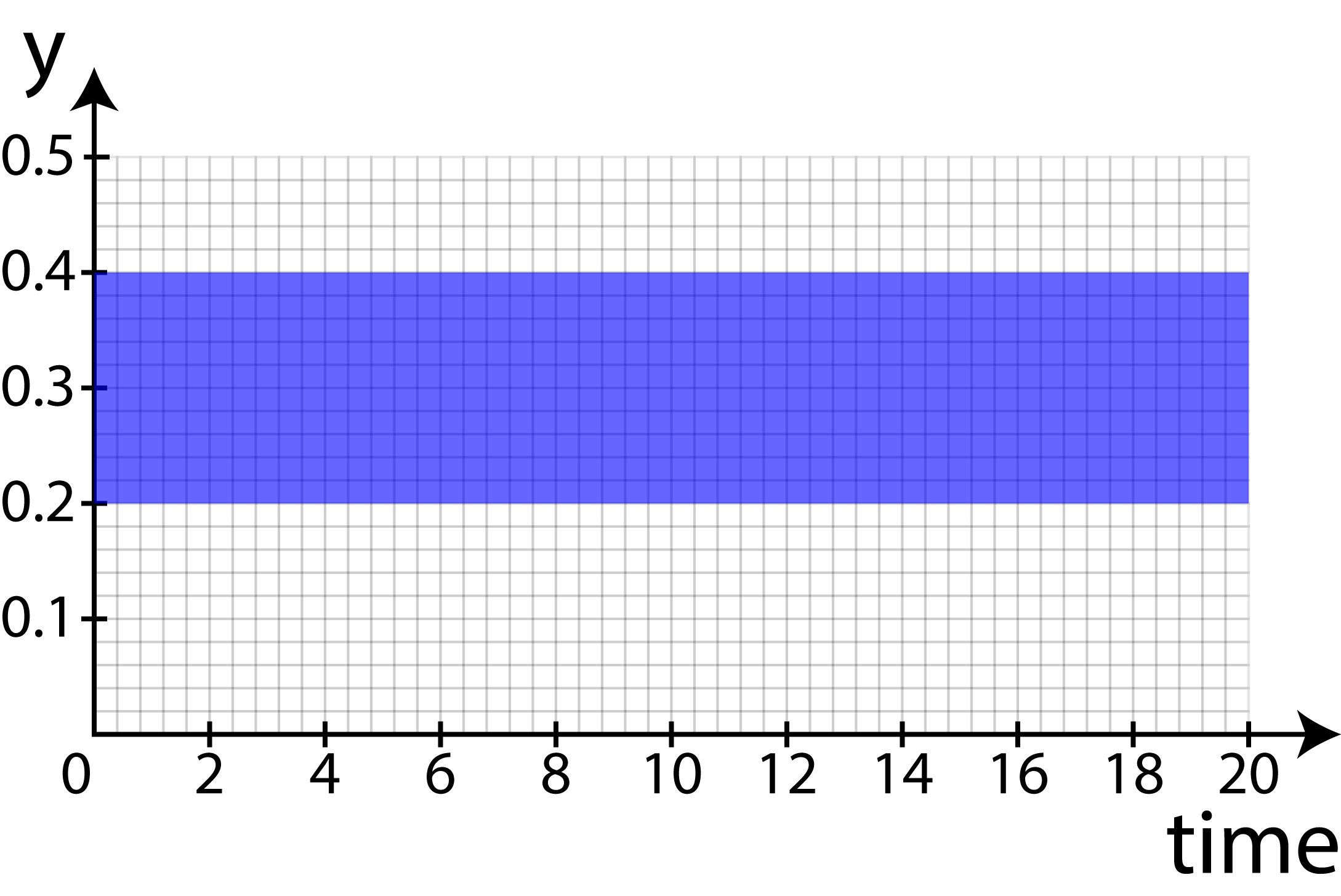
(a) $\phi_{1}$

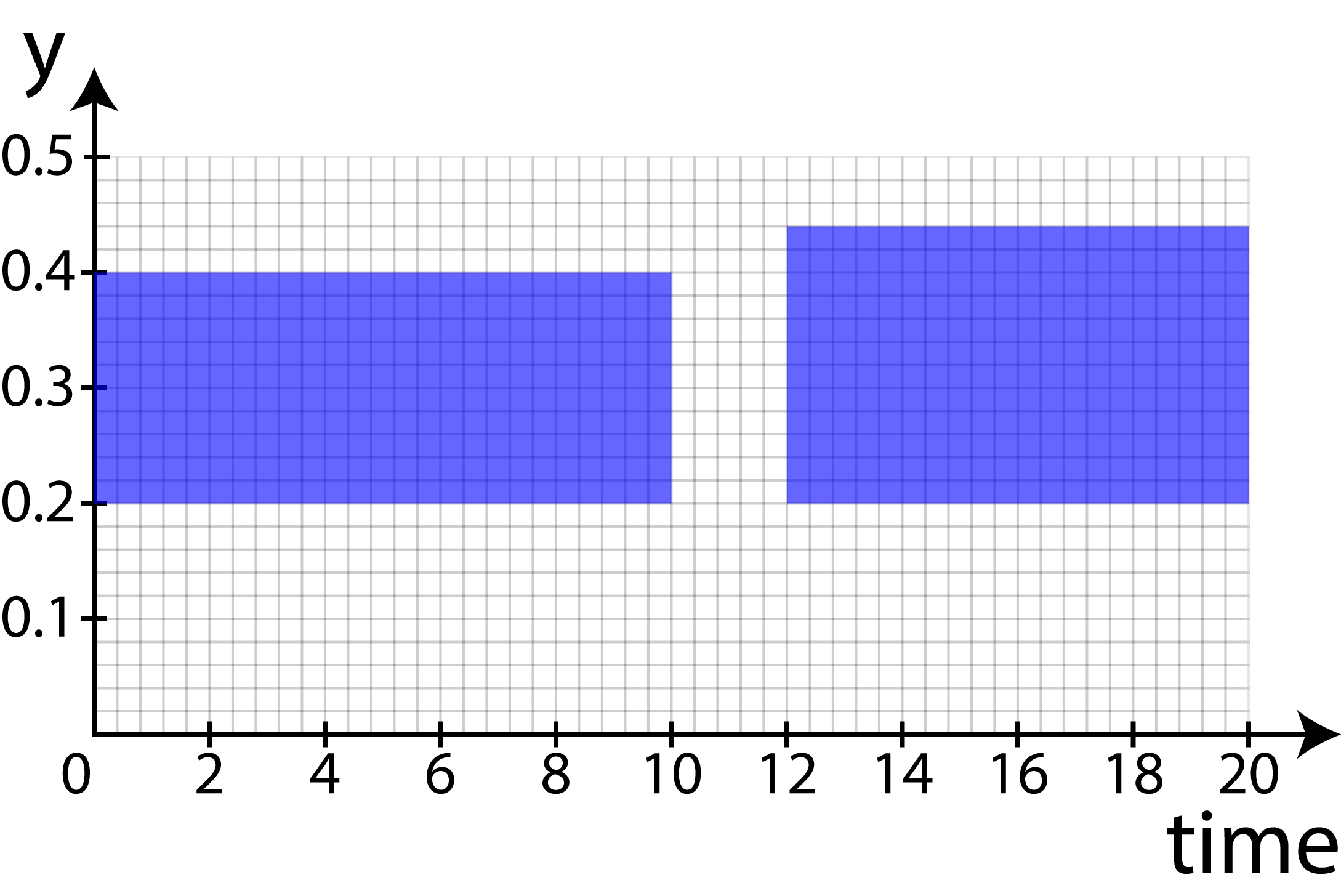
(b) $\phi_{5}$

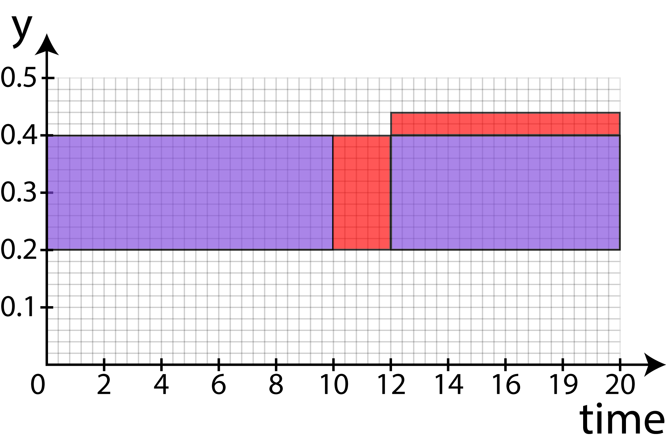
(c) Overlap $\phi_{1}$ and $\phi_{5}$

Figure 1: LABEL:sub@fig:phi1 and LABEL:sub@fig:phi5 show the area of satisfaction boxes for $\phi_{1}$ and $\phi_{5}$ from Example 2, respectively. The blue regions represent the boxes that are computed for globally ($\Box$) operators. In LABEL:sub@fig:overlap, the red regions represent the non-overlapping area and the purple regions represent the overlapping area between $\phi_{1}$ and $\phi_{5}$. The SD distance for this example is the area of the red regions ($(2\times 0.2)+(8\times 0.04)=0.72$) divided by the maximum time horizon which is $\frac{0.72}{20}=0.036$.

IV-B Symmetric Difference

This section presents an algorithm for computing boxes representing the area of satisfaction of a formula as well as a method for determining the SD between two sets of boxes. Each set of boxes approximates the projection ($\mathcal{P}$) of the formula and represents the valid value-space that a time-varying signal can take such that traces that are contained entirely within the boxes satisfy the formula.

Computing the set of boxes representing the area of satisfaction is a recursive process that takes as input an STL formula, $\phi$, a set of max values, $X_{max}$, for each signal, $x\in X$ (used to normalize the signal values to a unit space), and a discretization threshold, $\delta$. This algorithm, $AoS$, is presented in Algorithm 1 Here, $box(t_{1},t_{2},x_{1},x_{2},i)=\mathcal{P}(\Box_{[t_{1},t_{2}]}x_{1}\leq x^{i}\leq x_{2})\subseteq\mathbb{S}\times T\mathbb{U}$ creates a new box with minimum and maximum times $t_{1}$ and $t_{2}$, minimum and maximum values $x_{1}$ and $x_{2}$, and spatial dimension $i\in\{1,\ldots,n\}$, respectively; $overlap$ determines the time window of the overlap between two boxes; $combine$ takes two boxes and produces a set of boxes representing the intersection of the overlapping time window region; $b.lt$, $b.ut$, $b.lv\in\mathbb{S}$, and $b.uv\in\mathbb{S}$ return the lower time window, upper time window, lower variable, and upper variable values for box $b$, respectively; $*$ in the definition of a box denotes that it may restrict multiple spatial dimensions; and the $\parallel$ operator is used to create a “choice” set representing that either of the two sets separated by it can be selected as the set of boxes representing the area of satisfaction.

input : STL formula $\phi$, max value set $X_{max}$, discretization threshold $\delta$.

output : Set of boxes $\mathcal{B}$ for each signal in $\phi$.

if $\phi:=x^{i}\leq\pi$ then  return $box(0,0,0,\pi/x_{max},i)$

else if $\phi:=x^{i}>\pi$ then  return $box(0,0,\pi/x_{max},1,i)$

else if $\phi:=\phi_{1}\land\phi_{2}$ then

       Create a new set $\mathcal{B}$

       for each $b_{1}\in AoS(\phi_{1})$ and each $b_{2}\in AoS(\phi_{2})$ do

             if $overlap(b_{1},b_{2})$ then  Add $combine(b_{1},b_{2})$ to $\mathcal{B}$

             else  Add $b_{1}$ to $\mathcal{B}$ and $b_{2}$ to $\mathcal{B}$

            

      return $\mathcal{B}$

      

else if $\phi:=\phi_{1}\lor\phi_{2}$ then  return $AoS(\phi_{1})\parallel AoS(\phi_{2})$

else if $\phi:=\Box_{[t_{1},t_{2}]}(\phi_{1})$ then

       Create a new set $\mathcal{B}$

       for each $b\in AoS(\phi_{1})$ do

             $b^{\prime}=box(b.lt+t_{1},b.ut+t_{2},b.lv,b.uv,*)$

             Add $b^{\prime}$ to $\mathcal{B}$

            

      return $\mathcal{B}$

      

else if $\phi:=\diamondsuit_{[t_{1},t_{2}]}(\phi_{1})$ then

       return $AoS\left(\displaystyle\bigvee_{i=1}^{(t_{2}-t_{1})/\delta}\Box_{[t_{1}+\delta(i-1),t_{1}+\delta i]}(\phi_{1})\right)$

      

ALGORITHM 1 Convert to Area of Satisfaction Boxes ($AoS$)

To address the problem of projection of formulae containing disjunction (the converse to Theorem 1), $AoS$ utilizes the $\parallel$ operator. If this algorithm instead generated boxes representing the projection of all formulae, it would be possible for the satisfaction space represented by the boxes to capture signals that the original formula does not allow. The application in Section V highlights this problem and presents a way of dealing with it for that particular example.

For operators such as globally ($\Box$), $AoS$ is exact and produces boxes bound by the time bounds of the operator that represent the projection of the primitive. However, operators such as eventually ($\diamondsuit$) do not immediately lend themselves to conversion into a set of boxes. In order to deal with this operator, we approximate it by converting it into a disjunction of globally predicates. Each globally predicate is generated using a small threshold value ($\delta$) for its time window width. The new formula requires that the expression be true in at least one of the smaller time windows essentially introducing a mandatory $\delta$ “hold” time for eventually operators. The tunability of $\delta$ allows for a user to give up some accuracy for gains in performance of box computation and ultimately distance comparison. Examples of computing the area of satisfaction boxes for some of the formulae in Example 2 are shown in Figure 1.

The SD between two sets of boxes is computed by calculating the area of the sum of the non-intersected area for each box set. This value is normalized by the maximum time horizon, $T$, and results in the SD computation:

$$d_{SD}(\mathcal{B}_{\phi_{1}},\mathcal{B}_{\phi_{2}})=\frac{1}{T+1}\left|\left(\bigcup_{b_{1}\in\mathcal{B}_{\phi_{1}}}b_{1}\right)\triangle\left(\bigcup_{b_{2}\in\mathcal{B}_{\phi_{2}}}b_{2}\right)\right|$$

Figure 1c visually illustrates how the SD between $\phi_{1}$ and $\phi_{5}$ is computed.

Note that the SD distance is scaled by $\frac{T+1}{T^{\prime}+T+1}$ if the maximum horizon is increased by $T^{\prime}$. This again shows the temporal nature of the SD as opposed to the PH distance which does not change.

Complexity

The complexity of Algorithm 1 depends on the complexity of the $\parallel$ operation which may be exponential depending on how it is implemented. Otherwise, the algorithm is polynomial due to the box combination operations carried out whenever a conjunction predicate is encountered. In practice, computing the SD distance using this method for formulae with a few dozen predicates typically takes only a few seconds.

V Quantification of design quality

In our first application, we show an example of how the proposed metrics can be used in behavioral synthesis. Behavioral synthesis is an important process in design automation where the description of a desired behavior is interpreted and a system is created that implements the desired behavior. Our goal is to check if the characterized implementations satisfy the specifications of a system. Implementations include simulations and execution traces of a system. These implementations are characterized into formal specifications using TLI. We show that the proposed metrics can be used in the synthesis step to choose a design from the solution space that can best implement the desired specification. The specific example we have chosen to highlight this application is the synthesis of genetic circuits in synthetic biology.

Synthetic Genetic Circuit Synthesis

In this example, we have a set of desired behaviors (each formally represented by STL) which describe the various behaviors expected of a genetic circuit. This set of behaviors is referred to as a performance specification: $\mathcal{S}^{\phi}$. $\mathcal{S}^{\phi}$ consists of 2 STL formulae: $\phi_{low}$ and $\phi_{high}$ which describe the desired amount of output produced by the genetic circuit over time:

$$\phi_{low} = \>\>\Box_{[0,300]}(x<40)\land\Box_{[0,300]}(x>0)$$

$$\phi_{high} = \>\>\Box_{[0,125]}(x<200)\land\Box_{[125,300]}(x<320)\>\>\land$$

$$\>\>\Box_{[0,150]}(x>0)\land\Box_{[150,200]}(x>100)\>\>\land$$

$$\>\>\Box_{[200,300]}(x>150)$$

In this case, the output of the circuit corresponds to the expression of a fluorescent protein. $\phi_{low}$ specifies that the output must consistently be below 40 units from time 0 to 300, and $\phi_{high}$ specifies that that output must gradually increase over time and must end up between 150 and 320 units between time 200 and 300. Our solution space consists of two genetic circuits. The first circuit has a constitutive promoter as shown in Figure 2a. Constitutive expression removes flexibility for consistency allowing constant protein production independent of the state or inputs of the system, which is highlighted in Figure 2c. The second circuit has an inducible promoter: a sugar detecting transcription factor AraC*, which will turn on the protein production if and only if it is in the presence of a specific input molecule (arabinose) as shown in Figure 2b. Figure 2d shows the output of the circuit for various concentrations of arabinose. Both of these synthetic genetic circuits were built in Escherichia coli. The traces were obtained from biological experiments by measuring fluorescence.

(a) Constitutive Expression

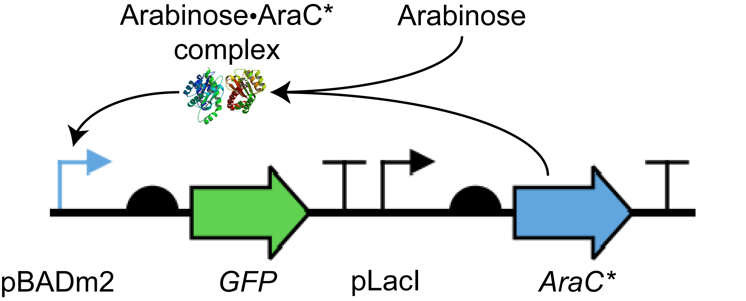
(b) Induction Circuit

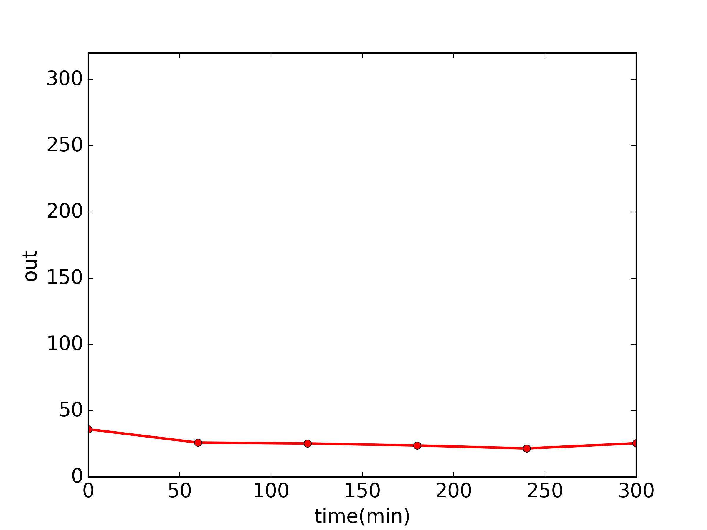
(c) Output of Constitutive Expression

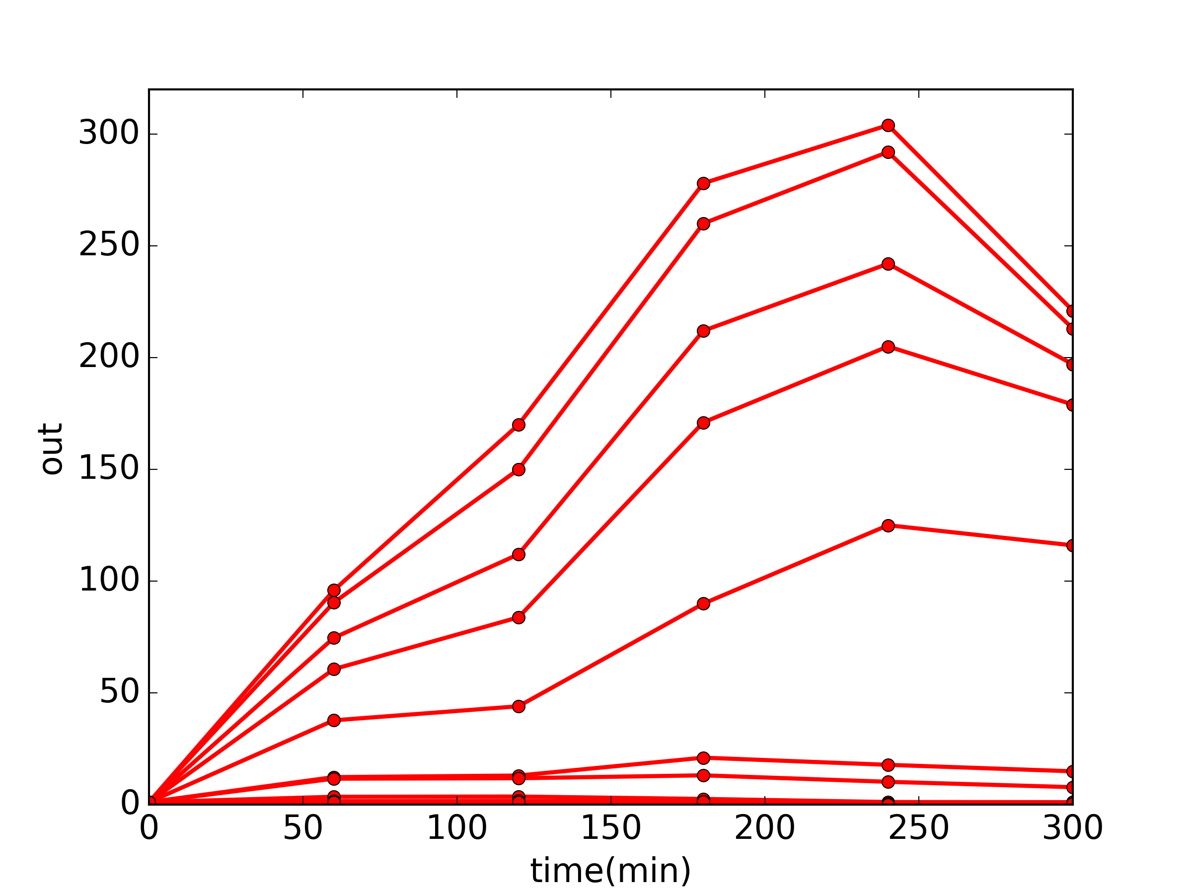
(d) Output of Induction Circuit

Figure 2: LABEL:sub@fig:constitutiveSBOL and LABEL:sub@fig:inductionSBOL show SBOL Visual representations of the genetic circuits with a constitutive promoter and an inducible promoter, respectively. Biological traces in LABEL:sub@fig:constitutiveExperiment and LABEL:sub@fig:inductionExperiment were obtained by evaluating geometric mean fluorescence at regular intervals by flow cytometry.

Our goal is to choose the circuit that can “satisfy as many behaviors as possible” in $\mathcal{S}^{\phi}$. It is important to note here that it is difficult to express the term “satisfy as many behaviors as possible” using the syntax and semantics of STL. For instance, expressing the desired specification as a disjunction of all the formulae in $\mathcal{S}^{\phi}$ would imply that satisfying any one specification is sufficient for the genetic circuit to satisfy the performance specification. Similarly, expressing the desired specification as a conjunction of all the formulae in $\mathcal{S}^{\phi}$ would imply that at any point in time, the output of a genetic circuit must have multiple distinct values, which is physically impossible.

This conundrum is highlighted in the current example. The output of constitutive expression satisfies $\phi_{low}$ but cannot satisfy $\phi_{high}$. The induction circuit produces traces that can satisfy both $\phi_{low}$ and $\phi_{high}$. However, traditional model checking techniques may not help a designer choose the desired circuit. Using statistical model checking, for example, the circuit with constitutive expression yields a satisfaction likelihood of $1.0$ and the induction circuit yields a satisfaction likelihood of $0.83$ when checked against $\phi_{low}\lor\phi_{high}$. With these results, one might think that the circuit with constitutive expression best satisfies the performance specification.

To address the issue of satisfying as many behaviors as possible, we treat the performance specification’s region of satisfaction as the union of the regions of satisfaction of all the formulae in $\mathcal{S}^{\phi}$ as shown in Figure 3a. We compute this region by taking the union of the generated boxes for each formula that are computed using Algorithm 1. The union of the box sets of all STL formulae in $\mathcal{S}^{\phi}$ is represented as $\mathcal{B}_{\phi_{low}}\cup\mathcal{B}_{\phi_{high}}=\mathcal{B}_{\mathcal{S}^{\phi}}$ and is shown in Figure 3b.

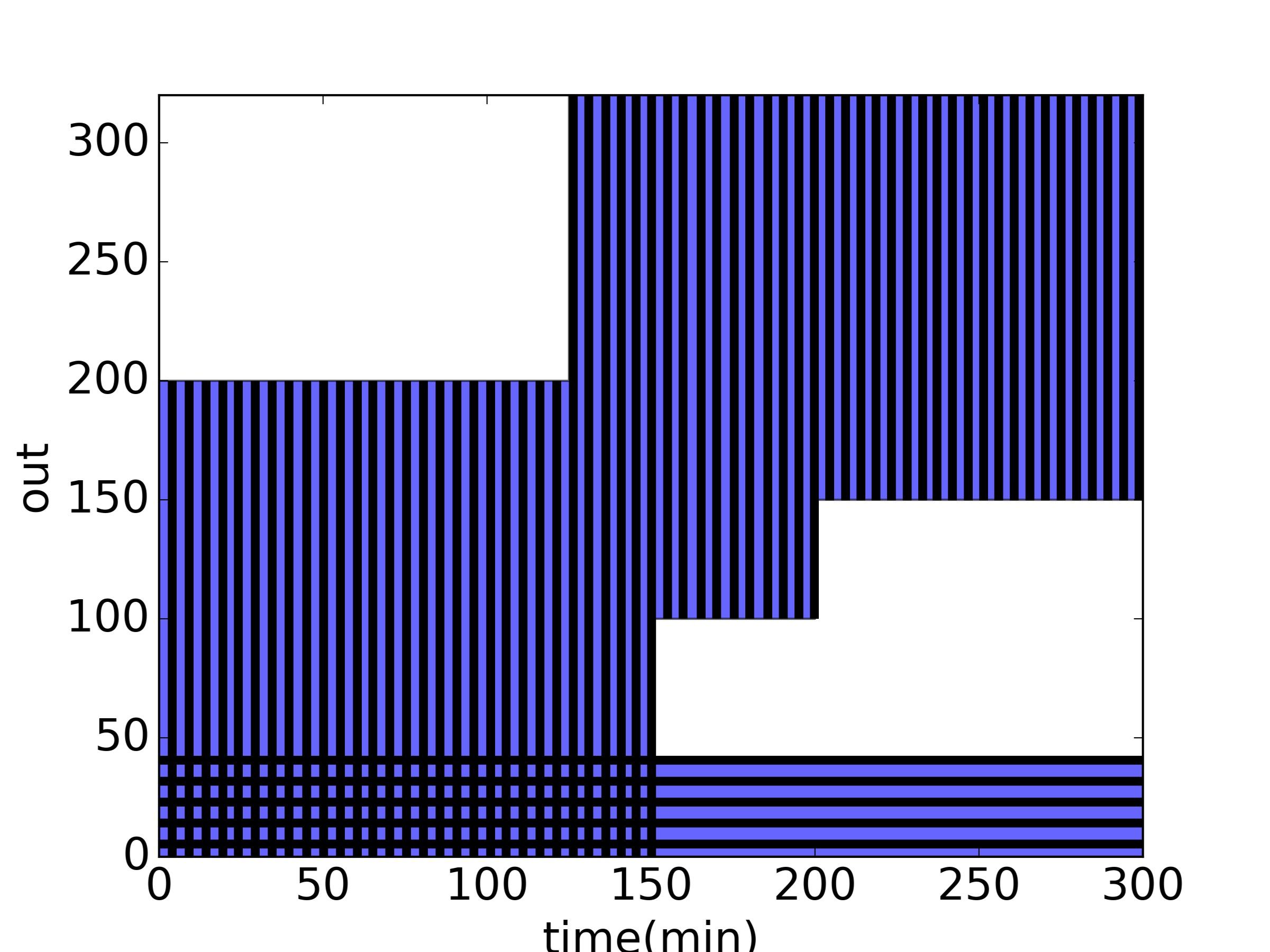
(a) $\mathcal{P}(\phi_{low}\lor\phi_{high})$

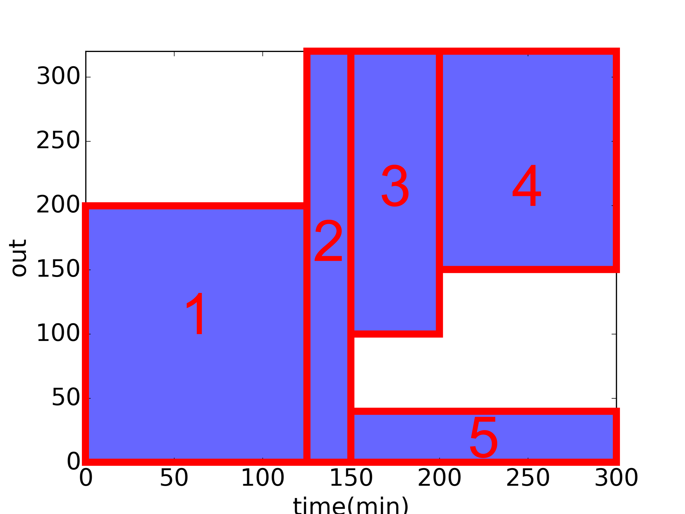
(b) $\mathcal{B}_{\phi_{low}}\cup\mathcal{B}_{\phi_{high}}=\mathcal{B}_{\mathcal{S}^{\phi}}$

Figure 3: LABEL:sub@fig:union shows the union of the areas of satisfaction for $\phi_{low}$ and $\phi_{high}$. The vertical stripe and horizontal stripe areas represent $\mathcal{P}(\phi_{low})$ and $\mathcal{P}(\phi_{high})$, respectively. LABEL:sub@fig:boxes shows the boxes created for $\mathcal{B}_{\phi_{low}}\cup\mathcal{B}_{\phi_{high}}$.

Using Grid TLI [22], we produce STL formulae, $\phi_{con}$ and $\phi_{ind}$, for each circuit using the traces shown in Figures 2c and 2d, respectively. We then use the SD metric and get the following values: $d_{SD}(\mathcal{B}_{\mathcal{S}^{\phi}},\mathcal{B}_{\phi_{con}})$ = $0.636$ and $d_{SD}(\mathcal{B}_{\mathcal{S}^{\phi}},\mathcal{B}_{\phi_{ind}})$ = $0.304$. Using the PH metric, we get: $d_{PH}(\mathcal{B}_{\mathcal{S}^{\phi}},\mathcal{B}_{\phi_{con}})$ = $0.067$ and $d_{PH}(\mathcal{B}_{\mathcal{S}^{\phi}},\mathcal{B}_{\phi_{ind}})$ = $0$. These results imply that the behavior of the induction circuit is closer to the desired specification than the circuit with constitutive expression, and thus, it should be selected as the desired circuit.

VI Loss functions for TLI

Loss functions play a fundamental role in statistical inference and learning theory. In this framework, we usually have a pair $(\mathcal{X},\mathcal{Y})$ of real vector spaces corresponding to the state and observation spaces, respectively. Three ingredients are used in the formalization: (a) a model of the states $p_{X}(x)$ – the prior distribution, (b) a model of the observations given the state $p_{Y\mid X}(y\mid x)$, and (c) a real-valued loss function $L:\mathcal{X}\times\mathcal{X}\to\mathbb{R}$. Let $h:\mathcal{Y}\to\mathcal{X}$ be a decision rule, which can also be interpreted as a partition of the state space $\mathcal{X}$ based on observations, and $\mathcal{H}$ be the set of all decision rules or the hypothesis space. The frequentist and Bayesian risks are defined based on the loss functions, and induce optimal decision rules. This general framework is the basis for the study and design of decision algorithms in statistical inference and learning. For more details, see [27].

In the following, we show how we adapt this framework for TLI, where we use the proposed metrics, PH and SD, as loss functions. In this paper, we only focus on the loss functions, while characterization of optimal decision rules, their computation, and regularization are left for future work.

For TLI, the state space $\mathcal{X}=\Phi^{\mathcal{S}_{T}}$ is the set of all time-bounded STL formulae, while the observation space $\mathcal{Y}=2^{\mathcal{S}_{T}}$ is the set of all languages. The hypothesis space $\mathcal{H}$ is composed of decision rules that map languages to STL formulae. Lastly, the loss functions are defined as $L_{STL}:\Phi^{\mathcal{S}_{T}}\times\Phi^{\mathcal{S}_{T}}\to\mathbb{R}$ such that $L_{STL}(\phi,h(S))$ represents the dissimilarity between the ground truth formula $\phi$ and the STL formula obtained by the decision rule using the signal set $S\subseteq\mathcal{S}_{T}$. We propose to use the PH and the SD metrics as loss functions $L_{STL}$.

We assess the performance of the two decision rules from TLI: TreeTLI [21] based on decision trees, and GridTLI [22] based on minimum covers of signals in space-time $\mathbb{S}\times[0,T]$, with respect to the two metrics as shown in Figure 4b.

The ground truth STL formula that was used to generate the signals in Figure 4a is

$$\phi_{GT}= \Box_{[0,1]}((x_{1}\leq 0.1)\land(x_{2}\leq 0.6)\land(x_{2}\geq 0.4))$$

$$\land\Box_{[7,10]}((x_{1}\geq 0.7)\land((x_{2}\geq 0.8)\lor(x_{2}\leq 0.2)))$$

where $\mathbb{S}=\mathbb{U}^{2}$ and $T=\left\|{\phi_{GT}}\right\|=10$. Note that TreeTLI requires both positive and negative examples, while GridTLI only needs positive ones. For brevity, we omit here the formalization for rules that require both types of examples.

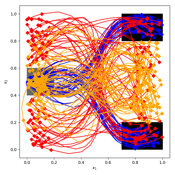
(a) Positive and Negative Signals

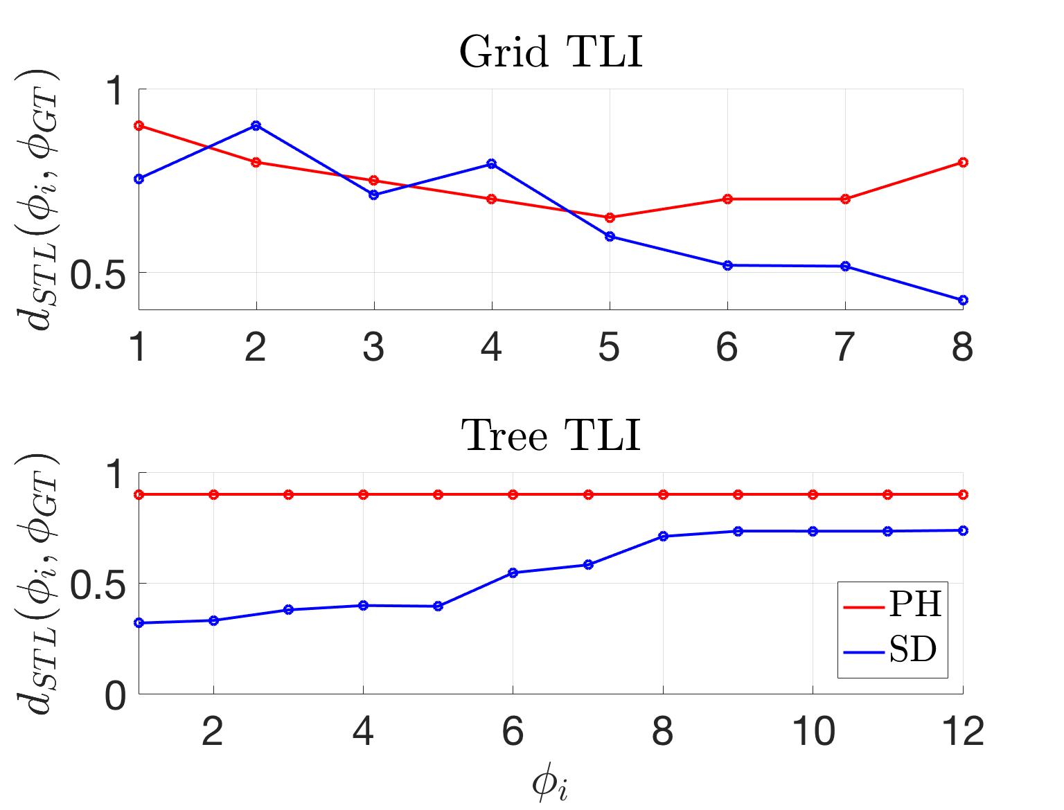
(b) Results

Figure 4: LABEL:sub@fig:tli-stat-learn-data shows the blue positive, and red and orange negative example signals used by the two TLI algorithms. The positive signals start in the gray region, and end in one of the black regions. The red negative signals do not start in the gray region, while the orange ones do not end in the black regions. LABEL:sub@fig:tli-stat-learn-results shows the PH and the SD distances between the ground truth formula $\phi_{GR}$ and the learned formulae using GridTLI and TreeTLI, respectively.

The results in Figure 4b show the distances between the ground truth formula $\phi_{GT}$ and the iterations of TreeTLI (lower plot) as the decision tree grows [21]. For GridTLI (upper plot), we varied the discretization thresholds [22] from rougher to finer grids, $\delta_{s}\in\{0.5,0.45,\ldots,0.1\}$ and $\delta_{t}\in\{5,4.5,\ldots,1\}$ for space and time, respectively. The upper plot for GridTLI highlights the over-fitting phenomenon in the PH metric (red), where reducing the discretization thresholds helps reducing the error, but further reduction leads to over-fitting. For the SD (blue), the loss has a decreasing trend which we hypothesize is due to a better temporal fitting that the PH distance does not capture. In the case of TreeTLI (lower plot), the PH distance (red) is constant. This masking behavior might be due to the compounding effect of i) the primitives used do not match the structure of $\phi_{GT}$, and ii) the incremental and local nature of TreeTLI. Thus, the first step of the decision tree is heavily penalized by the PH metric. The SD metric (blue), which shows an increasing trend, is consistent with this conclusion.

Thus, the statistical learning approach to TLI gives insight into the ability of algorithms to recover temporal logic rules assumed to underlie data. It also provides a formal framework to study TLI methods. A detailed account of problems GridTLI and TreeTLI are appropriate for based on the insights provided by the proposed metrics is left for future work.

VII Discussion and Future Work

We presented two metrics for computing the distance of one STL formula to another. These methods are very useful in applications where temporal logic specifications are mined from simulation or experimental data, and need to be compared against a desired specification. Fields such as synthetic biology and robotics, where systems are characterized with performance specifications, can greatly benefit from our methods. We also showed how these metrics are useful as a first step in evaluating the performance of TLI methods.

An immediate theoretical extension is studying continuous-time signals. By assuming Lipschitz continuity of signals, it is possible to provide bounds between the metrics computed in discrete-time and the ones in continuous-time. A similar idea was used in [8] to compute sampled-time STL scores. The second extension is relaxing the assumption on rectangular predicates.

References

- [1] C. Baier and J. Katoen, Principles of model checking. MIT Press, 2008.
- [2] H. Kress-Gazit, G. E. Fainekos, and G. J. Pappas, “Temporal-logic-based reactive mission and motion planning,” IEEE transactions on robotics, vol. 25, no. 6, pp. 1370–1381, 2009.
- [3] G. Batt, B. Yordanov, R. Weiss, and C. Belta, “Robustness analysis and tuning of synthetic gene networks,” Bioinformatics, vol. 23, no. 18, pp. 2415–2422, 2007.
- [4] S. Coogan, M. Arcak, and C. Belta, “Formal methods for control of traffic flow: Automated control synthesis from finite-state transition models,” IEEE Control Systems, vol. 37, no. 2, pp. 109–128, 2017.
- [5] E. A. Emerson and E. M. Clarke, “Using branching time temporal logic to synthesize synchronization skeletons,” Science of Computer Programming, vol. 2, no. 3, pp. 241 – 266, 1982.
- [6] A. Pnueli, “The temporal logic of programs,” in Foundations of Computer Science, 1977., 18th Annual Symposium on. IEEE, 1977, pp. 46–57.
- [7] O. Maler and D. Nickovic, “Monitoring temporal properties of continuous signals,” in Formal Techniques, Modelling and Analysis of Timed and Fault-Tolerant Systems. Springer, 2004, pp. 152–166.
- [8] G. E. Fainekos and G. J. Pappas, “Robustness of temporal logic specifications for continuous-time signals,” Theoretical Computer Science, vol. 410, no. 42, pp. 4262–4291, 2009.
- [9] A. Donzé and O. Maler, Robust satisfaction of temporal logic over real-valued signals. Springer, 2010.
- [10] A. Donzé, T. Ferrere, and O. Maler, “Efficient robust monitoring for STL,” in Computer Aided Verification. Springer, 2013, pp. 264–279.
- [11] J. Tumova, L. Reyes-Castro, S. Karaman, E. Frazzoli, and D. Rus, “Minimum-violating planning with conflicting specifications,” in American Control Conference (ACC), 2013.
- [12] J. Tumova, G. C. Hall, S. Karaman, E. Frazzoli, and D. Rus, “Least-violating control strategy synthesis with safety rules,” in International Conference on Hybrid Systems: Computation and Control, Philadelphia, PA, USA, 2013, pp. 1–10.
- [13] C.-I. Vasile, J. Tumova, S. Karaman, C. Belta, and D. Rus, “Minimum-violation scLTL motion planning for mobility-on-demand,” in IEEE International Conference on Robotics and Automation, Singapore, Singapore, May 2017, pp. 1481–1488.
- [14] C. I. Vasile, D. Aksaray, and C. Belta, “Time Window Temporal Logic,” Theoretical Computer Science, vol. 691, no. Supplement C, pp. 27–54, August 2017.
- [15] K. Kim, G. Fainekos, and S. Sankaranarayanan, “On the minimal revision problem of specification automata,” The International Journal of Robotics Research, 2015.
- [16] S. Ghosh, D. Sadigh, P. Nuzzo, V. Raman, A. Donzé, A. L. Sangiovanni-Vincentelli, S. S. Sastry, and S. A. Seshia, “Diagnosis and repair for synthesis from signal temporal logic specifications,” in Proc. International Conference on Hybrid Systems: Computation and Control. ACM, 2016, pp. 31–40.
- [17] J. R. Munkres, Topology. Prentice Hall, 2000.
- [18] J. B. Conway, A course in abstract analysis. American Mathematical Soc., 2012, vol. 141.
- [19] E. Bartocci, L. Bortolussi, and G. Sanguinetti, “Data-driven statistical learning of temporal logic properties,” in Formal Modeling and Analysis of Timed Systems, A. Legay and M. Bozga, Eds. Cham: Springer International Publishing, 2014, pp. 23–37.
- [20] X. Jin, A. Donzé, J. V. Deshmukh, and S. A. Seshia, “Mining requirements from closed-loop control models,” IEEE Transactions on Computer-Aided Design of Integrated Circuits and Systems, vol. 34, no. 11, pp. 1704–1717, 2015.
- [21] G. Bombara, C.-I. Vasile, F. Penedo, H. Yasuoka, and C. Belta, “A Decision Tree Approach to Data Classification Using Signal Temporal Logic,” in Proc. International Conference on Hybrid Systems: Computation and Control. New York, NY, USA: ACM, 2016, pp. 1–10.
- [22] P. Vaidyanathan, R. Ivison, G. Bombara, N. A. DeLateur, R. Weiss, D. Densmore, and C. Belta, “Grid-based temporal logic inference,” in Annual Conference on Decision and Control (CDC). IEEE, 2017, pp. 5354–5359.
- [23] B. Hoxha, A. Dokhanchi, and G. Fainekos, “Mining parametric temporal logic properties in model-based design for cyber-physical systems,” International Journal on Software Tools for Technology Transfer, vol. 20, no. 1, pp. 79–93, Feb 2018.
- [24] A. Dokhanchi, B. Hoxha, and G. Fainekos, 5th International Conference on Runtime Verification, Toronto, ON, Canada. Springer, 2014, ch. On-Line Monitoring for Temporal Logic Robustness, pp. 231–246.
- [25] D. Kraft, “Computing the Hausdorff distance of two sets from their signed distance functions,” Computational Geometry, Submitted March 2015.
- [26] V. Raman, A. Donzé, M. Maasoumy, R. M. Murray, A. Sangiovanni-Vincentelli, and S. A. Seshia, “Model predictive control with signal temporal logic specifications,” in Decision and Control (CDC), 2014 IEEE 53rd Annual Conference on. IEEE, 2014, pp. 81–87.
- [27] V. Vapnik, The nature of statistical learning theory. Springer, 2013.