Published in the Elsevier journal “Physica D: Nonlinear Phenomena”, Volume 404, March 2020: Special Issue on Machine Learning and Dynamical Systems Fundamentals of Recurrent Neural Network (RNN) and Long Short-Term Memory (LSTM) Network

Abstract

Because of their effectiveness in broad practical applications, LSTM networks have received a wealth of coverage in scientific journals, technical blogs, and implementation guides. However, in most articles, the inference formulas for the LSTM network and its parent, RNN, are stated axiomatically, while the training formulas are omitted altogether. In addition, the technique of “unrolling” an RNN is routinely presented without justification throughout the literature. The goal of this tutorial is to explain the essential RNN and LSTM fundamentals in a single document. Drawing from concepts in Signal Processing, we formally derive the canonical RNN formulation from differential equations. We then propose and prove a precise statement, which yields the RNN unrolling technique. We also review the difficulties with training the standard RNN and address them by transforming the RNN into the “Vanilla LSTM” network through a series of logical arguments. We provide all equations pertaining to the LSTM system together with detailed descriptions of its constituent entities. Albeit unconventional, our choice of notation and the method for presenting the LSTM system emphasizes ease of understanding. As part of the analysis, we identify new opportunities to enrich the LSTM system and incorporate these extensions into the Vanilla LSTM network, producing the most general LSTM variant to date. The target reader has already been exposed to RNNs and LSTM networks through numerous available resources and is open to an alternative pedagogical approach. A Machine Learning practitioner seeking guidance for implementing our new augmented LSTM model in software for experimentation and research will find the insights and derivations in this treatise valuable as well.

0

I Introduction

Since the original 1997 LSTM paper [21], numerous theoretical and experimental works have been published on the subject of this type of an RNN, many of them reporting on the astounding results achieved across a wide variety of application domains where data is sequential. The impact of the LSTM network has been notable in language modeling, speech-to-text transcription, machine translation, and other applications [31]. Inspired by the impressive benchmarks reported in the literature, some readers in academic and industrial settings decide to learn about the Long Short-Term Memory network (henceforth, “the LSTM network”) in order to gauge its applicability to their own research or practical use-case. All major open source machine learning frameworks offer efficient, production-ready implementations of a number of RNN and LSTM network architectures. Naturally, some practitioners, even if new to the RNN/LSTM systems, take advantage of this access and cost-effectiveness and proceed straight to development and experimentation. Others seek to understand every aspect of the operation of this elegant and effective system in greater depth. The advantage of this lengthier path is that it affords an opportunity to build a certain degree of intuition that can prove beneficial during all phases of the process of incorporating an open source module to suit the needs of their research effort or a business application, preparing the dataset, troubleshooting, and tuning.

In a common scenario, this undertaking balloons into reading numerous papers, blog posts, and implementation guides in search of an “A through Z” understanding of the key principles and functions of the system, only to find out that, unfortunately, most of the resources leave one or more of the key questions about the basics unanswered. For example, the Recurrent Neural Network (RNN), which is the general class of a neural network that is the predecessor to and includes the LSTM network as a special case, is routinely simply stated without precedent, and unrolling is presented without justification. Moreover, the training equations are often omitted altogether, leaving the reader puzzled and searching for more resources, while having to reconcile disparate notation used therein. Even the most oft-cited and celebrated primers to date have fallen short of providing a comprehensive introduction. The combination of descriptions and colorful diagrams alone is not actionable, if the architecture description is incomplete, or if important components and formulas are absent, or if certain core concepts are left unexplained.

As of the timeframe of this writing, a single self-contained primer that provides a clear and concise explanation of the Vanilla LSTM computational cell with well-labeled and logically composed schematics that go hand-in-hand with the formulas is still lacking. The present work is motivated by the conviction that a unifying reference, conveying the basic theory underlying the RNN and the LSTM network, will benefit the Machine Learning (ML) community.

The present article is an attempt to fill in this gap, aiming to serve as the introductory text that the future students and practitioners of RNN and LSTM network can rely upon for learning all the basics pertaining to this rich system. With the emphasis on using a consistent and meaningful notation to explain the facts and the fundamentals (while removing mystery and dispelling the myths), this backgrounder is for those inquisitive researchers and practitioners who not only want to know “how”, but also to understand “why”.

We focus on the RNN first, because the LSTM network is a type of an RNN, and since the RNN is a simpler system, the intuition gained by analyzing the RNN applies to the LSTM network as well. Importantly, the canonical RNN equations, which we derive from differential equations, serve as the starting model that stipulates a perspicuous logical path toward ultimately arriving at the LSTM system architecture.

The reason for taking the path of deriving the canonical RNN equations from differential equations is that even though RNNs are expressed as difference equations, differential equations have been indispensable for modeling neural networks and continue making a profound impact on solving practical data processing tasks with machine learning methods. On one hand, leveraging the established mathematical theories from differential equations in the continuous-time domain has historically led to a better understanding of the evolution of the related difference equations, since the difference equations are obtained from the corresponding original differential equations through discretization of the differential operators acting on the underlying functions [57, 59, 30, 20, 33, 54, 61, 60]. On the other hand, considering the existing deep neurally-inspired architectures as the numerical methods for solving their respective differential equations aided by the recent advances in memory-efficient implementations has helped to successfully stabilize very large models at lower computational costs compared to their original versions [9, 4, 3]. Moreover, differential equations defined on the continuous time domain are a more natural fit for modeling certain real-life scenarios than the difference equations defined over the domain of evenly-discretized time intervals [6, 51].

Our primary aspiration for this document, particularly for the sections devoted to the Vanilla LSTM system and its extensions, is to fulfill all of the following requirements:

1. Intuitive – the notation and semantics of variables must be descriptive, explicitly and unambiguously mapping to their respective purposes in the system.

2. Complete – the explanations and derivations must include both the inference equations (“forward pass” or “normal operation”) and the training equations (“backward pass”), and account for all components of the system.

3. General – the treatment must concern the most inclusive form of the LSTM system (i.e., the “Vanilla LSTM”), specifically including the influence of the cell’s state on control nodes (“pinhole connections”).

4. Illustrative – the description must include a complete and clearly labeled cell diagram as well as the sequence diagram, leaving nothing to imagination or guessing (i.e., the imperative is: strive to minimize cognitive strain, do not leave anything as an “exercise for the reader” – everything should be explained and made explicit).

5. Modular – the system must be described in such a way that the LSTM cell can be readily included as part of a pluggable architecture, both horizontally (“deep sequence”) and vertically (“deep representation”).

6. Vector notation – the equations should be expressed in the matrix and vector form; it should be straightforward to plug the equations into a matrix software library (such as $\mathtt{numpy}$) as written, instead of having to iterate through indices.

In all sources to date, one or more of the elements in the above list is not addressed [13, 14, 15, 68, 66, 16, 69, 55, 32, 27, 40, 42, 26, 78, 50, 5, 35, 34, 36, 24, 56]. Hence, to serve as a comprehensive introduction, the present tutorial captures all the essential details. The practice of using a succinct vector notation and meaningful variable names as well as including the intermediate steps in formulas is designed to build intuition and make derivations easy to follow.

The rest of this document is organized as follows. Section II gives a principled background behind RNN systems. Then
Section III formally arrives at RNN unrolling by proving a precise statement concerning approximating long sequences by a series of shorter, independent sub-sequences (segments). Section IV presents the RNN training mechanism based on the technique, known as “Back Propagation Through Time”, and explores the numerical difficulties, which occur when training on long sequences. To remedy these problems, Section V methodically constructs the Vanilla LSTM cell from the canonical RNN system (derived in Section II) by reasoning through the ways of making RNN more robust. Section VI provides a detailed explanation of all aspects of the Vanilla LSTM cell. Even though this section is intended to be self-contained, familiarity with the material covered in the preceding sections will be beneficial. The Augmented LSTM system, which embellishes the Vanilla LSTM system with the new computational components, identified as part of the exercise of transforming the RNN to the LSTM network, is presented in Section VII. Section VIII summarizes the covered topics and proposes future projects.

II The Roots of RNN

In this section, we will derive the Recurrent Neural Network (RNN) from differential equations [61, 60]. Let $\vec{s}(t)$ be the value of the $d$-dimensional state signal vector and consider the general nonlinear first-order non-homogeneous ordinary differential equation, which describes the evolution of the state signal as a function of time, $t$:

$$\frac{d\vec{s}(t)}{dt} =\vec{f}(t)+\vec{\phi}$$ (1)

where $\vec{f}(t)$ is a $d$-dimensional vector-valued function of time, $t\in\mathbb{R}^{+}$, and $\vec{\phi}$ is a constant $d$-dimensional vector.

One canonical form of $\vec{f}(t)$ is:

$$\vec{f}(t) =\vec{h}\left(\vec{s}(t),\vec{x}(t)\right)$$ (2)

where $\vec{x}(t)$ is the $d$-dimensional input signal vector and $\vec{h}\left(\vec{s}(t),\vec{x}(t)\right)$ is a vector-valued function of vector-valued arguments.

The resulting system,

$$\frac{d\vec{s}(t)}{dt} =\vec{h}\left(\vec{s}(t),\vec{x}(t)\right)+\vec{\phi}$$ (3)

comes up in many situations in physics, chemistry, biology, and engineering [65, 72].

In certain cases, one starts with $s$ and $x$ as entirely “analog” quantities (i.e., functions not only of time, $t$, but also of another independent continuous variable, $\vec{\xi},$ denoting the coordinates in multi-dimensional space). Using this notation, the intensity of an input video signal displayed on a flat $2$-dimensional screen would be represented as $x(\vec{\xi},t)$ with $\vec{\xi}\in\mathbb{R}^{2}$. Sampling $x(\vec{\xi},t)$ on a uniform $2$-dimensional grid converts this signal to the representation $x(\vec{i},t)$, where $\vec{i}$ is now a discrete $2$-dimensional index. Finally, assembling the values of $x(\vec{i},t)$ for all permutations of the components of the index, $\vec{i}$, into a column vector, produces $\vec{x}(t)$ as originally presented in Equation 3 above.

One special case of $\vec{f}(t)$ in Equation 2 is:

$$\vec{f}(t) =\vec{a}(t)+\vec{b}(t)+\vec{c}(t)$$ (4)

whose constituent terms, $\vec{a}(t)$, $\vec{b}(t)$, and $\vec{c}(t)$, are $d$-dimensional vector-valued functions of time, $t$. Equation 4 is called the “Additive Model” in Brain Dynamics research literature, because it adds the terms, possibly nonlinear, that determine the rate of change of neuronal activities, or potentials, $\vec{s}(t)$. As a cornerstone of neural network research, the abstract form of the Additive Model in Equation 4 has been particularized in many ways, including incorporating the effects of delays, imposing “shunting” (or “saturating”) bounds on the state of the system, and other factors. Biologically motivated uses of the Additive Model span computational analyses of vision, decision making, reinforcement learning, sensory-motor control, short-term and long-term memory, and the learning of temporal order in language and speech [18]. It has also been noted that the Additive Model generalizes the Hopfield model [23], which, while rooted in biological plausibility, has been influential in physics and engineering [19, 18]. In fact, a simplified and discretized form of the Additive Model played a key role in linking the nonlinear dynamical systems governing morphogenesis, one of the fundamental aspects of developmental biology, to a generalized version of the Hopfield network [23], and applying it to an engineering problem in image processing [59, 62].

Consider a saturating Additive Model in Equation 4 with the three constituent terms, $\vec{a}(t)$, $\vec{b}(t)$, and $\vec{c}(t)$, defined as follows:

$$\vec{a}(t) =\sum_{k=0}^{K_{s}-1}\vec{a}_{k}(\vec{s}(t-\tau_{s}(k)))$$ (5)

$$\vec{b}(t) =\sum_{k=0}^{K_{r}-1}\vec{b}_{k}(\vec{r}(t-\tau_{r}(k)))$$ (6)

$$\vec{r}(t-\tau_{r}(k)) =G\left(\vec{s}(t-\tau_{r}(k))\right)$$ (7)

$$\vec{c}(t) =\sum_{k=0}^{K_{x}-1}\vec{c}_{k}(\vec{x}(t-\tau_{x}(k)))$$ (8)

where $\vec{r}(t)$, the readout signal vector, is a warped version of the state signal vector, $\vec{s}(t)$. A popular choice for the element-wise nonlinear, saturating, and invertible “warping” (or “activation”) function, $G(z)$, is an optionally scaled and/or shifted form of the hyperbolic tangent. Then the resulting system, obtained by substituting Equations 5 – 8 into Equation 4 and inserting into Equation 1, becomes:

$$\frac{d\vec{s}(t)}{dt} =\sum_{k=0}^{K_{s}-1}\vec{a}_{k}(\vec{s}(t-\tau_{s}(k)))+\sum_{k=0}^{K_{r}-1}\vec{b}_{k}(\vec{r}(t-\tau_{r}(k)))+\sum_{k=0}^{K_{x}-1}\vec{c}_{k}(\vec{x}(t-\tau_{x}(k)))+\vec{\phi}$$ (9)

$$\vec{r}(t-\tau_{r}(k)) =G\left(\vec{s}(t-\tau_{r}(k))\right)$$ (10)

Equation 9 is a nonlinear ordinary delay differential equation (DDE) with discrete delays. Delay is a common feature of many processes in biology, chemistry, mechanics, physics, ecology, and physiology, among others, whereby the nature of the processes dictates the use of delay equations as the only appropriate means of modeling. In engineering, time delays often arise in feedback loops involving sensors and actuators [28].

Hence, the time rate of change of the state signal in Equation 9 depends on three main components plus the constant (“bias”) term, $\vec{\phi}$. The first (“analog”) component, $\sum_{k=0}^{K_{s}-1}\vec{a}_{k}(\vec{s}(t-\tau_{s}(k)))$, is the combination of up to $K_{s}$ time-shifted (by the delay time constants, $\tau_{s}(k)$) functions, $\vec{a}_{k}(\vec{s}(t))$, where the term “analog” underscores the fact that each $\vec{a}_{k}(\vec{s}(t))$ is a function of the (possibly time-shifted) state signal itself (i.e., not the readout signal, which is the warped version of the state signal). The second component, $\sum_{k=0}^{K_{r}-1}\vec{b}_{k}(\vec{r}(t-\tau_{r}(k)))$, is the combination of up to $K_{r}$ time-shifted (by the delay time constants, $\tau_{r}(k)$) functions, $\vec{b}_{k}(\vec{r}(t))$, of the readout signal, given by Equation 10, the warped (binary-valued in the extreme) version of the state signal. The third component, $\sum_{k=0}^{K_{x}-1}\vec{c}_{k}(\vec{x}(t-\tau_{x}(k)))$, representing the external input, is composed of the combination of up to $K_{x}$ time-shifted (by the delay time constants, $\tau_{x}(k)$) functions, $\vec{c}_{k}(\vec{x}(t))$, of the input signal.

The rationale behind choosing a form of the hyperbolic tangent as the warping function is that the hyperbolic tangent possesses certain useful properties. On one hand, it is monotonic and negative-symmetric with a quasi-linear region, whose slope can be regulated [38]. On the other hand, it is bipolarly-saturating (i.e., bounded at both the negative and the positive limits of its domain). The quasi-linear mode aides in the design of the system’s parameters and in interpreting its behavior in the “small signal” regime (i.e., when $\left\|\vec{s}(t)\right\|\ll 1)$. The bipolarly-saturating (“squashing”) aspect, along with the proper design of the internal parameters of the functions $\vec{a}_{k}(\vec{s}(t))$ and $\vec{b}_{k}(\vec{r}(t))$, helps to keep the state of the system (and, hence, its output) bounded. The dynamic range of the state signals is generally unrestricted, but the readout signals are guaranteed to be bounded, while still carrying the state information with low distortion in the quasi-linear mode of the warping function (the “small signal” regime). If the system, described by Equation 9 and Equation 10, is stable, then the state signals are bounded as well [64].

The time delay terms on the right hand side of Equation 9 comprise the “memory” aspects of the system. They enable the quantity holding the instantaneous time rate of change of the state signal, $\frac{d\vec{s}(t)}{dt}$, to incorporate contributions from the state, the readout, and the input signal values, measured at different points in time, relative to the current time, $t$. Qualitatively, these temporal elements enrich the expressive power of the model by capturing causal and/or contextual information.

In neural networks, the time delay is an intrinsic part of the system and also one of the key factors that determines the dynamics. Much of the pioneering research in recurrent networks during the 1970s and the 1980s was founded on the premise that neuron processes and interactions could be expressed as systems of coupled DDEs [23, 18]. Far from the actual operation of the human brain, based on what was already known at the time, these “neurally inspired” mathematical models have been shown to exhibit sufficiently interesting emerging behaviors for both, advancing the knowledge and solving real-world problems in various practical applications. While the major thrust of research efforts was concerned primarily with continuous-time networks, it was well understood that the learning procedures could be readily adapted to discrete systems, obtained from the original differential equations through sampling. We will also follow the path of sampling and discretization for deriving the RNN equations [60]. Over the span of these two decades, pivotal and lasting contributions were made in the area of training networks containing interneurons with “Error Back Propagation” (or “Back Propagation of Error”, or “Back Propagation” for short), a special case of a more general error gradient computation procedure. To accommodate recurrent networks, both continuous-time and discrete-time versions of “Back Propagation Through Time” have been developed on the foundation of Back Propagation and used to train the weights and time delays of these networks to perform a wide variety of tasks [25, 47, 48, 45, 11, 46]. We will rely on Back Propagation Through Time for training the systems analyzed in this paper.

The contribution of each term on the right hand side of Equation 9 to the overall system is qualitatively different from that of the others. The functions, $\vec{a}_{k}(\vec{s}(t-\tau_{s}(k)))$, of the (“analog”) state signal in the first term have a strong effect on the stability of the system, while the functions, $\vec{b}_{k}(\vec{r}(t-\tau_{r}(k)))$, of the (bounded) readout signal in the second term capture most of the interactions that shape the system’s long-term behavior. If warranted by the modeling requirements of the biological or physical system and/or of the specific datasets and use-cases in an engineering setting, the explicit inclusion of non-zero delay time constants in these terms provides the necessary weighting flexibility in the temporal domain (e.g., to account for delayed neural interactions) [10]. Thus, the parameters, $K_{s}$, $K_{r}$, and $K_{x}$ representing the counts of the functions, $\vec{a}_{k}(\vec{s}(t-\tau_{s}(k)))$, $\vec{b}_{k}(\vec{r}(t-\tau_{r}(k)))$, and $\vec{c}_{k}(\vec{x}(t-\tau_{x}(k)))$, respectively (and the counts of the associated delay time constants, $\tau_{s}(k)$, $\tau_{r}(k)$, and $\tau_{x}(k)$, respectively, of these functions), in the system equations are chosen (or estimated by an iterative procedure) accordingly.

Suppose that $\vec{a}_{k}(\vec{s}(t-\tau_{s}(k)))$, $\vec{b}_{k}(\vec{r}(t-\tau_{r}(k)))$, and $\vec{c}_{k}(\vec{x}(t-\tau_{x}(k)))$ are linear functions of $\vec{s}$, $\vec{r}$, and $\vec{x}$, respectively. Then Equation 9 becomes a nonlinear DDE with linear (matrix-valued) coefficients:

$$\frac{d\vec{s}(t)}{dt} =\sum_{k=0}^{K_{s}-1}A_{k}(\vec{s}(t-\tau_{s}(k)))+\sum_{k=0}^{K_{r}-1}B_{k}(\vec{r}(t-\tau_{r}(k)))+\sum_{k=0}^{K_{x}-1}C_{k}(\vec{x}(t-\tau_{x}(k)))+\vec{\phi}$$ (11)

Furthermore, if the matrices, $A_{k}$, $B_{k}$, and $C_{k}$, are circulant (or block circulant), then the matrix-vector multiplication terms in Equation 11 can be expressed as convolutions in the space of the elements of $\vec{s}$, $\vec{r}$, $\vec{x}$, and $\vec{\phi}$, each indexed by $\vec{i}$:

$$\frac{ds(\vec{i},t)}{dt} =\sum_{k=0}^{K_{s}-1}a_{k}(\vec{i})\ast s(\vec{i},t-\tau_{s}(k))+\sum_{k=0}^{K_{r}-1}b_{k}(\vec{i})\ast r(\vec{i},t-\tau_{r}(k))+\sum_{k=0}^{K_{x}-1}c_{k}(\vec{i})\ast x(\vec{i},t-\tau_{x}(k))+\phi(\vec{i})$$ (12)

The index, $\vec{i}$, is $1$-dimensional if the matrices, $A_{k}$, $B_{k}$, and $C_{k}$, are circulant and multi-dimensional if they are block circulant.

The summations of time delayed terms in Equation 12 represent convolutions in the time domain with finite-sized kernels, consisting of the spatial convolutions $a_{k}(\vec{i})\ast s(\vec{i})$, $b_{k}(\vec{i})\ast r(\vec{i})$, and $c_{k}(\vec{i})\ast x(\vec{i})$ as the coefficients for the three temporal components, respectively. In fact, if the entire data set (e.g., the input data set, $\vec{x}(t)$) is available a priori for all time ahead of the application of Equation 12, then some of the corresponding time delays (e.g., $\tau_{x}(k)$) can be negative, thereby allowing the incorporation of “future” information for computing the state of the system at the present time, $t$. This will become relevant further down in the analysis.

Before proceeding, it is interesting to note that earlier studies linked the nonlinear dynamical system, formalized in Equation 9 (with $K_{s}=K_{r}=K_{x}=1$ and all $\tau_{s}$, $\tau_{r}$, and $\tau_{x}$ set to zero), to the generalization of a type of neural networks. Specifically the variant, in which the functions $\vec{a}_{k}(\vec{s}(t))$, $\vec{b}_{k}(\vec{r}(t))$, and $\vec{c}_{k}(\vec{x}(t))$ are linear operators as in Equation 11 (with $K_{s}=K_{r}=K_{x}=1$ and all $\tau_{s}$, $\tau_{r}$, and $\tau_{x}$ set to zero) was shown to include the Continuous Hopfield Network [23] as a special case. Its close relative, in which these operators are further restricted to be convolutional as in Equation 12 (again, with $K_{s}=K_{r}=K_{x}=1$ and all $\tau_{s}$, $\tau_{r}$, and $\tau_{x}$ set to zero), was shown to include the Cellular Neural Network [8, 7] as a special case [59, 64, 62].

Applying the simplifications:

$$\begin{rcases}K_{s}&=1\\ \tau_{s}(0)&=0\\ A_{0}&=A\\ K_{r}&=1\\ \tau_{r}(0)&=\tau_{0}\\ B_{0}&=B\\ K_{x}&=1\\ \tau_{x}(0)&=0\\ C_{0}&=C\end{rcases}$$ (13)

(some of which will be later relaxed) to Equation 11 turns it into:

$$\frac{d\vec{s}(t)}{dt} =A\vec{s}(t)+B\vec{r}(t-\tau_{0})+C\vec{x}(t)+\vec{\phi}$$ (14)

Equation 11, Equation 12, and, hence, Equation 14 are nonlinear first-order non-homogeneous DDEs. A standard numerical technique for evaluating these equations, or, in fact, any embodiments of Equation 1, is to discretize them in time and compute the values of the input signals and the state signals at each time sample up to the required total duration, thereby performing numerical integration.

Denoting the duration of the sampling time step as $\triangle T$ and the index of the time sample as $n$ in the application of the backward Euler discretization rule to Equation 14 yields:

$$t =n\triangle T$$ (15)

$$\frac{d\vec{s}(t)}{dt} \thickapprox\frac{\vec{s}(n\triangle T+\triangle T)-\vec{s}(n\triangle T)}{\triangle T}$$ (16)

$$A\vec{s}(t)+B\vec{r}(t-\tau_{0})+C\vec{x}(t)+\vec{\phi} =A\vec{s}(n\triangle T)+B\vec{r}(n\triangle T-\tau_{0})+C\vec{x}(n\triangle T)+\vec{\phi}$$ (17)

$$A\vec{s}(t+\triangle T)+B\vec{r}(t+\triangle T-\tau_{0})+C\vec{x}(t+\triangle T)+\vec{\phi} =A\vec{s}(n\triangle T+\triangle T)+B\vec{r}(n\triangle T+\triangle T-\tau_{0})+C\vec{x}(n\triangle T+\triangle T)+\vec{\phi}$$ (18)

$$\frac{\vec{s}(n\triangle T+\triangle T)-\vec{s}(n\triangle T)}{\triangle T} \thickapprox A\vec{s}(n\triangle T+\triangle T)+B\vec{r}(n\triangle T+\triangle T-\tau_{0})+C\vec{x}(n\triangle T+\triangle T)+\vec{\phi}$$ (19)

Now set the delay, $\tau_{0}$, equal to the single time step. This can be interpreted as storing the value of the readout signal into memory at every time step to be used in the above equations at the next time step. After a single use, the memory storage can be overwritten with the updated value of the readout signal to be used at the next time step, and so forth. Thus, setting $\tau_{0}=\triangle T$ and replacing the approximation sign with an equal sign for convenience in Equation 19 gives:

$$\frac{\vec{s}(n\triangle T+\triangle T)-\vec{s}(n\triangle T)}{\triangle T} =A\vec{s}(n\triangle T+\triangle T)+B\vec{r}(n\triangle T)+C\vec{x}(n\triangle T+\triangle T)+\vec{\phi}$$ (20)

$$\frac{\vec{s}((n+1)\triangle T)-\vec{s}(n\triangle T)}{\triangle T} =A\vec{s}((n+1)\triangle T)+B\vec{r}(n\triangle T)+C\vec{x}((n+1)\triangle T)+\vec{\phi}$$ (21)

$$\vec{s}((n+1)\triangle T)-\vec{s}(n\triangle T) =\triangle T\left(A\vec{s}((n+1)\triangle T)+B\vec{r}(n\triangle T)+C\vec{x}((n+1)\triangle T)+\vec{\phi}\right)$$ (22)

After performing the discretization, all measurements of time in Equation 22 become integral multiples of the sampling time step, $\triangle T$. Now, $\triangle T$ can be dropped from the arguments, which leaves the time axis dimensionless. Hence, all the signals are transformed into sequences, whose domain is the discrete index, $n$, and Equation 14 turns into a nonlinear first-order non-homogeneous difference equation [1]:

$$\vec{s}[n+1]-\vec{s}[n] =\triangle T\left(A\vec{s}[n+1]+B\vec{r}[n]+C\vec{x}[n+1]+\vec{\phi}\right)$$ (23)

$$\vec{s}[n+1] =\vec{s}[n]+\triangle T\left(A\vec{s}[n+1]+B\vec{r}[n]+C\vec{x}[n+1]+\vec{\phi}\right)$$

$$\left(I-(\triangle T)A\right)\vec{s}[n+1] =\vec{s}[n]+\left((\triangle T)B\right)\vec{r}[n]+\left((\triangle T)C\right)\vec{x}[n+1]+(\triangle T)\vec{\phi}$$ (24)

Defining:

$$W_{s} =\left(I-(\triangle T)A\right)^{-1}$$ (25)

and multiplying both sides of Equation 24 by $W_{s}$ leads to:

$$\vec{s}[n+1] =W_{s}\vec{s}[n]+\left((\triangle T)W_{s}B\right)\vec{r}[n]+\left((\triangle T)W_{s}C\right)\vec{x}[n+1])+\left((\triangle T)W_{s}\vec{\phi}\right)$$

which after shifting the index, $n$, forward by $1$ step becomes:

$$\vec{s}[n] =W_{s}\vec{s}[n-1]+\left((\triangle T)W_{s}B\right)\vec{r}[n-1]+\left((\triangle T)W_{s}C\right)\vec{x}[n]+\left((\triangle T)W_{s}\vec{\phi}\right)$$

$$\vec{r}[n] =G(\vec{s}[n])$$ (26)

Defining two additional weight matrices and a bias vector,

$$W_{r} =(\triangle T)W_{s}B$$ (27)

$$W_{x} =(\triangle T)W_{s}C$$ (28)

$$\vec{\theta}_{s} =(\triangle T)W_{s}\vec{\phi}$$ (29)

transforms the above system into the canonical Recurrent Neural Network (RNN) form:

$$\vec{s}[n] =W_{s}\vec{s}[n-1]+W_{r}\vec{r}[n-1]+W_{x}\vec{x}[n]+\vec{\theta}_{s}$$ (30)

$$\vec{r}[n] =G(\vec{s}[n])$$ (31)

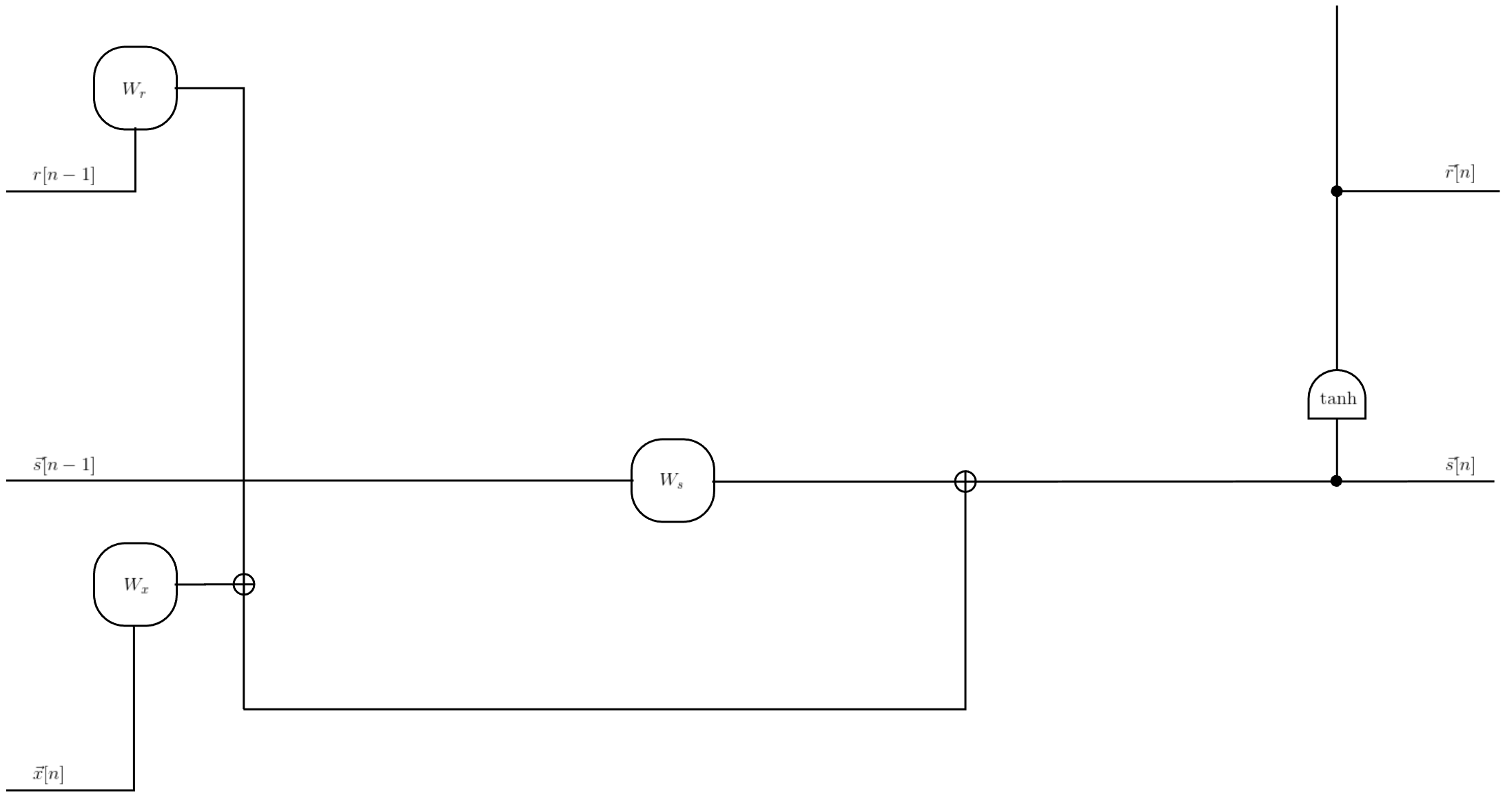
Figure 1: Canonical RNN cell. The bias parameters, $\vec{\theta}_{s},$ have been omitted from the figure for brevity. It can be assumed to be included without the loss of generality by appending an additional element, always set to $1$, to the input signal vector, $\vec{x}[n]$, and increasing the row dimensions of $W_{x}$ by $1$.

The RNN formulation in Equation 30, diagrammed in Figure 1, will be later logically evolved into the LSTM system. Before that, it is beneficial to introduce the process of “unrolling” and the notion of a “cell” of an RNN. These concepts will be simpler to describe using the standard RNN definition, which is derived next from Equation 30 based on stability arguments.

For the system in Equation 30 to be stable, every eigenvalue of $\hat{W}=W_{s}+W_{r}$ must lie within the complex-valued unit circle [1, 65]. Since there is considerable flexibility in the choice of the elements of $A$ and $B$ to satisfy this requirement, setting $\triangle T=1$ for simplicity is acceptable. As another simplification, let $A$ be a diagonal matrix with large negative entries (i.e., $a_{ii}\ll 0$) on its main diagonal (thereby practically guaranteeing the stability of Equation 14). Then, from Equation 25, $W_{s}\thickapprox-A^{-1}$ will be a diagonal matrix with small positive entries, $\frac{1}{\left|a_{ii}\right|}$, on its main diagonal, which means that the explicit effect of the state signal’s value from memory, $\vec{s}[n-1]$, on the system’s trajectory will be negligible (the implicit effect through $\vec{r}[n-1]$ will still be present as long as $\left\|W_{r}\right\|>0$). Thus, ignoring the first term in Equation 30, reduces it to the standard RNN definition:

$$\vec{s}[n] =W_{r}\vec{r}[n-1]+W_{x}\vec{x}[n]+\vec{\theta}_{s}$$ (32)

$$\vec{r}[n] =G(\vec{s}[n])$$ (33)

From Equation 32, now only the matrix $\hat{W}\thickapprox W_{r}\thickapprox-A^{-1}B$ is responsible for the stability of the RNN. Consider the best case scenario, where $B$ is a diagonal matrix ($B=\Lambda_{B}$). With this simplification, the essential matrix for analyzing the stability of Equation 32 becomes $\tilde{W}=-A^{-1}\Lambda_{B}$, where $\Lambda_{B}$ is the diagonal matrix (i.e., consisting of only the eigenvalues of $B$, with the individual eigenvalues, $\lambda_{i}$, on the main diagonal of $\Lambda_{B}$). Since both $A$ and $\Lambda_{B}$ are diagonal, $\tilde{W}$ is a diagonal matrix with the entries $\mu_{i}=\frac{\lambda_{i}}{\left|a_{ii}\right|}$ on its main diagonal. These quantities become the eigenvalues of the overall RNN system in Equation 32 in the “small signal regime” ($\left\|\vec{s}[n]\right\|\ll 1)$, each adding the mode of $\left(\mu_{i}\right)^{n}$, multiplied by its corresponding initial condition, to the trajectory of $\vec{s}[n]$. A necessary and sufficient condition for stability is that $0<\mu_{i}<1$, meaning that every eigenvalue, $\lambda_{i}$, of $B$ must satisfy the condition $0<\lambda_{i}<\left|a_{ii}\right|$. If any $\mu_{i}$ and $\lambda_{i}$ fail to satisfy this condition, the system will be unstable, causing the elements of $\vec{r}[n]$ to either oscillate or saturate (i.e., enter the flat regions of the warping nonlinearity) at some value of the index, $n$.

An alternative to choosing the specific convenient form of $A$ in Equation 25 would be to (somewhat arbitrarily) treat $W_{s}$, $W_{r}$, $W_{x}$, and $\vec{\theta}_{s}$ in Equation 30 as mutually independent parameters and then set $W_{s}=0$ to obtain the standard RNN definition (as in Equation 32). In this case, the above stability analysis still applies. In particular, the eigenvalues, $\mu_{i}$, of $W_{r}$ are subject to the same requirement, $0<\mu_{i}<1$, as a necessary and sufficient condition for stability.

Stability considerations will be later revisited in order to justify the need to evolve the RNN to a more complex system, namely, the LSTM network.

We have shown that the RNN, as expressed by Equation 30 (in the canonical form) or by Equation 32 (in the standard form), essentially implements the backward Euler numerical integration method for the ordinary DDE in Equation 14. This “forward” direction of starting in the continuous-time domain (differential equation) and ending in the discrete-index domain (difference equation) implies that the original phenomenon being modeled is assumed to be fundamentally analog in nature, and that it is modeled in the discrete domain as an approximation for the purpose of realization. For example, the source signal could be the audio portion of a lecture, recorded on an analog tape (or on digital media as a finely quantized waveform and saved in an audio file). The original recording thus contains the spoken words as well as the intonation, various emphases, and other vocal modulations that communicate the content in the speaker’s individual way as expressed through voice. The samples generated by a hypothetical discretization of this phenomenon, governed in this model by Equation 14, could be captured as the textual transcript of the speech, saved in a document containing only the words uttered by the speaker, but ignoring all the intonation, emotion, and other analogous nuances. In this scenario, it is the sequence of words in the transcript of the lecture that the RNN will be employed to reproduce, not the actual audio recording of the speech. The key subtle point in this scenario is that applying the RNN as a model implies that the underlying phenomenon is governed by Equation 14, whereby the role of the RNN is that of implementing the computational method for solving this DDE using the backward Euler discretization rule, under the restriction that the sampling time step, $\triangle T$, is equal to the delay, $\tau_{0}$. In contrast, the “reverse” direction would be a more appropriate model in situations where the discrete signal is the natural starting domain, because the phenomenon originates as a sequence of samples. For example, a written essay originates as a sequence of words and punctuation, saved in a document. One can conjure up an analog rendition of this essay as being read by a narrator, giving life to the words and passages with intonation, pauses, and other expressions not present in the original text of the essay. While the starting point depends on how the original source of data is generated, both the continuous (“forward”) and the discrete (“reverse”) representations can serve as tools for gaining insight into the advantages and the limitations of the models under consideration.

III RNN Unfolding/Unrolling

It is convenient to use the term “cell” when referring to Equation 30 and Equation 32 in the uninitialized state. In other words, the sequence has been defined by these equations, but its terms not yet computed. Then the cell can be said to be “unfolded” or “unrolled” by specifying the initial conditions on the state signal, $\vec{s}[n]$, and numerically evaluating Equation 30 or
Equation 32 for a finite range of discrete steps, indexed by $n$. This process is illustrated in Figure 2.

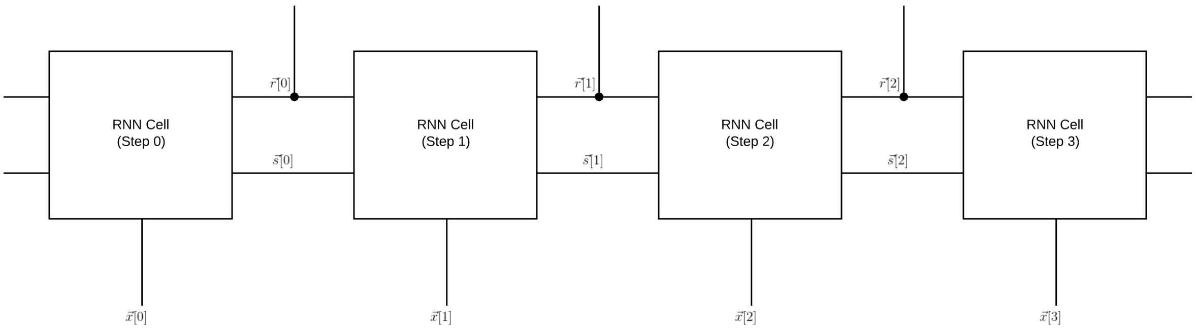
Figure 2: Sequence of steps generated by unrolling an RNN cell.

Both Equation 30 and Equation 32 are recursive in the state signal, $\vec{s}[n]$. Hence, due to the repeated application of the recurrence relation as part of the unrolling, the state signal, $\vec{s}[n]$, at some value of the index, $n$, no matter how large, encompasses the contributions of the state signal, $\vec{s}[k]$, and the input signal, $\vec{x}[k]$, for all indices, $k<n$, ending at $k=0$, the start of the sequence [25, 11]. Because of this attribute, the RNN belongs to the category of the “Infinite Impulse Response” (IIR) systems.

Define the vector-valued unit step function as:

$$\vec{u}[n] =\begin{cases}\vec{1},&n\geq 0\\ \vec{0},&n<0\end{cases}$$ (34)

where $\vec{0}$ and $\vec{1}$ denote vectors, all of whose elements are equal to $0$ and to $1$, respectively. Then the vector-valued unit sample function, $\vec{\delta}[n]$, is defined by being $\vec{1}$ at $n=0$, and $\vec{0}$ otherwise. In terms of $\vec{u}[n]$,

$$\vec{\delta}[n] =\vec{u}[n]-\vec{u}[n-1]$$ (35)

These functions are depicted in Figure 3.

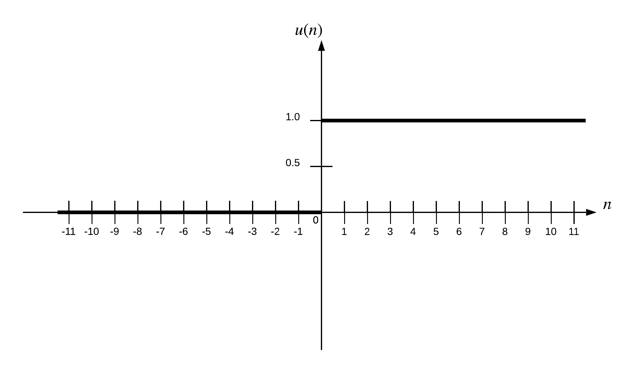
(a) The unit step function.

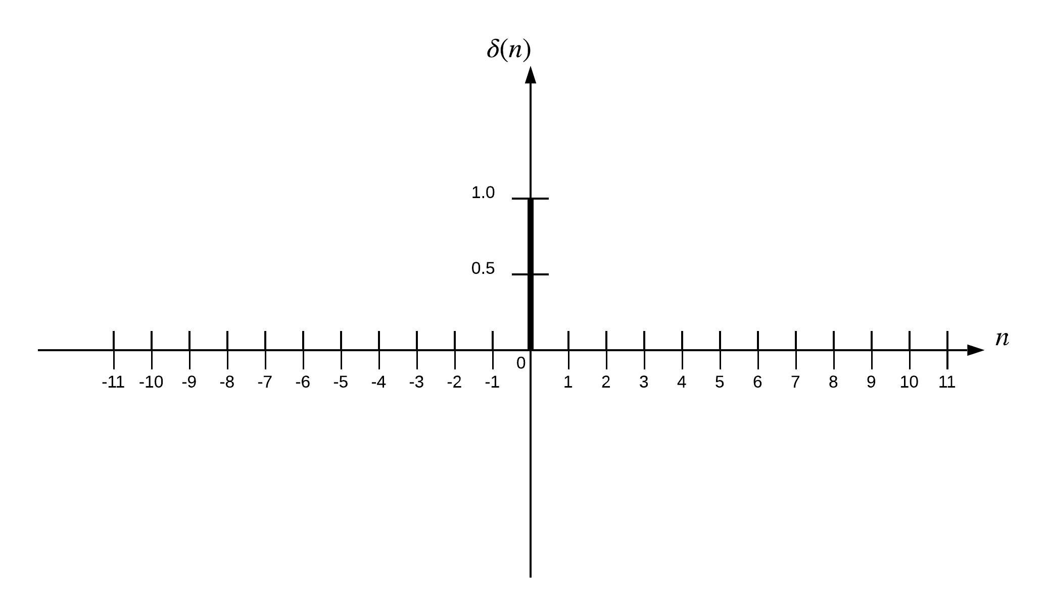
(b) The unit sample function.

Figure 3: The unit step and the unit sample (“impulse”) functions plotted (in one data dimension) against the discrete index, $n$.

Example 1.

The IIR (i.e., unending) nature of the sequences, governed by these equations, can be readily demonstrated by letting $\vec{s}[-1]=\vec{0}$ be the initial condition, setting $\vec{x}[n]=\vec{\delta}[n]$, the unit sample stimulus (i.e., the “impulse”), and computing the response, $\vec{s}[n]$, to this “impulse” for several values of the index, $n$, in order to try to recognize a pattern. In the case of Equation 32 with $\vec{\theta}_{s}=\vec{0}$, the sequence of $\vec{s}[n]$ values will be:

$$\vec{s}[n=-1] =\vec{0}$$

$$\vec{s}[n=0] =W_{x}\vec{1}$$

$$\vec{s}[n=1] =W_{r}G(W_{x}\vec{1})$$

$$\vec{s}[n=2] =W_{r}G(W_{r}G(W_{x}\vec{1}))$$

$$\vec{s}[n=3] =W_{r}G(W_{r}G(W_{r}G(W_{x}\vec{1})))$$

$$\vec{s}[n=4] =W_{r}G(W_{r}G(W_{r}G(W_{r}G(W_{x}\vec{1}))))$$

$$\cdots$$ (36)

and so forth. Evidently, it is defined for every positive $n$, even when the input is only a single impulse at $n=0$.

In practice, it is desirable to approximate a sequence with an infinite support (IIR), such as Equation 30 or Equation 32, by a “Finite Impulse Response” (FIR) sequence. The rationale is that FIR systems have certain advantages over IIR systems. One advantage is guaranteed stability – FIR systems are intrinsically stable. Another advantage is that FIR systems are realizable with finite computational resources. An FIR system will take a finite number of steps to compute the output from the input and will require a finite number of memory locations for storing intermediate results and various coefficients. Moreover, the computational complexity and storage requirements of an FIR system are known at design time.

Denote the sequence of the “ground truth” output values by $\vec{v}[n]$ for any value of the index, $n$, and let $N$ be the length of the sequence, $\vec{v}[n]$, where $N$ can be an arbitrarily large integer (e.g., the total number of samples in the training set, or the number of inputs presented to the system for inference over the lifetime of the system, etc.). Suppose that $\vec{v}[n]\left\rfloor{}_{0\leq n\leq N-1}\right.$ is subdivided into $M$ non-overlapping varying-length segments with $K_{m}$ samples per segment, where every $K_{m}$ is finite, and $K_{m}\leq N$. It can be assumed that $M$ is an integer with $M\geq 1$ (if needed, the RNN system in Equation 32 can be “padded” with extra $\vec{x}[n]=\vec{0}$ input terms for this to hold).

Formally, let $\vec{v}[n]\left\rfloor{}_{0\leq n\leq N-1}\right.$ be the sequence of the ground truth output values for any value of the index, $n$, and assume that there exists a partitioning of $\vec{v}[n]\left\rfloor{}_{0\leq n\leq N-1}\right.$ into $M$ non-overlapping segments, $\vec{v}_{m}[n]$, $0\leq m\leq M-1$:

$$\vec{v}[n]\left\rfloor{}_{0\leq n\leq N-1}\right. =\sum_{m=0}^{M-1}\vec{v}_{m}[n]$$ (37)

For subdividing a sequence into $M$ non-overlapping segments, consider a vector-valued “rectangular” window function, $\vec{w}_{0}[n]$, which has the value of $\vec{1}$ within the window $0\leq n\leq K_{0}-1$ and $\vec{0}$ otherwise. In terms of the vector-valued unit step function, $\vec{u}[n]$, $\vec{w}_{0}[n]$ is defined as:

$$\vec{w}_{0}[n] =\vec{u}[n]-\vec{u}[n-K_{0}]$$ (38)

Combining Equation 35 with Equation 38 provides an alternative (“sampling”) definition of $\vec{w}_{0}[n]$:

$$\vec{w}_{0}[n] =\vec{u}[n]-\vec{u}[n-1]$$

$$+\vec{u}[n-1]-\vec{u}[n-2]$$

$$+\vec{u}[n-2]-\vec{u}[n-3]$$

$$+\ldots+$$

$$+\vec{u}[n-(K_{0}-2)]-\vec{u}[n-(K_{0}-1)]$$

$$+\vec{u}[n-(K_{0}-1)]-\vec{u}[n-K_{0}]$$

$$=\sum_{k=0}^{K_{0}-1}\vec{\delta}[n-k]$$ (39)

Then from Equation 39, the RNN sequence can be sampled in its entirety by the full $N$-samples-long window:

$$\vec{w}[n] =\vec{u}[n]-\vec{u}[n-N]$$

$$=\sum_{m=0}^{M-1}\left(\sum_{k=j(m)}^{j(m)+K_{m}-1}\vec{\delta}[n-k]\right)$$ (40)

$$=\sum_{m=0}^{M-1}\vec{w}_{m}[n]$$ (41)

where:

$$j(m) =\begin{cases}\sum_{i=0}^{m-1}K_{i},&1\leq m\leq M-1\\ 0,&m=0\end{cases}$$ (42)

and:

$$\vec{w}_{m}[n] =\sum_{k=j(m)}^{j(m)+K_{m}-1}\vec{\delta}[n-k]$$ (43)

Under the change of indices,

$$l =k-j(m)$$

$$k =j(m)+l$$

$$l \longrightarrow k$$

Equation 43 becomes:

$$\vec{w}_{m}[n] =\sum_{k=0}^{K_{m}-1}\vec{\delta}[n-j(m)-k]$$ (44)

Equation 44 indicates that each $\vec{w}_{m}[n]$ is a rectangular window, whose size is $K_{m}$ samples. Hence, “extracting” a
$K_{m}$-samples-long segment with the index, $m$, from the overall ground truth output sequence, $\vec{v}[n]\left\rfloor{}_{0\leq n\leq N-1}\right.$, amounts to multiplying this sequence by $\vec{w}_{m}[n]$:

$$\vec{v}_{m}[n]\left\rfloor{}_{0\leq n\leq N-1}\right. =\vec{w}_{m}[n]\odot\vec{v}[n]\left\rfloor{}_{0\leq n\leq N-1}\right.$$ (45)

$$=\begin{cases}\vec{v}[n],&j(m)\leq n\leq j(m)+K_{m}-1\\ \vec{0},&\textrm{otherwise}\end{cases}$$ (46)

where $j(m)$ is given by Equation 42. According to Equation 46, the segment-level ground truth output subsequence,
$\vec{v}_{m}[n]\left\rfloor{}_{0\leq n\leq N-1}\right.$, in Equation 45 will have non-zero values for the given value of the segment index, $m$, where $0\leq m\leq M-1$, only when the index, $n$, is in the range $j(m)\leq n\leq j(m)+K_{m}-1$. This is in agreement with Equation 37.

Define $\mathcal{Q}(\left\langle\vec{r}[n]\right\rangle)$ as an invertible map that transforms an ensemble of the readout signals of the RNN system, $\left\langle\vec{r}[n]\right\rangle$, into an ensemble of observable output signals, $\left\langle\vec{y}[n]\right\rangle$, for $0\leq n\leq N-1$:

$$\left\langle\vec{y}[n]\right\rangle \equiv\mathcal{Q}(\left\langle\vec{r}[n]\right\rangle)$$ (47)

In addition, define $\mathcal{L}$ as an “objective function” (or “merit function” [71]) that measures the cost of the observable output of the system deviating from the desired ground truth output values, given the input data, supplied over the entire range of the values of the index, $n$:

$$\mathcal{L}\left(\left\langle\vec{y}[n]\right\rangle\left\rfloor{}_{0\leq n\leq N-1}\right.,\left\langle\vec{v}[n]\right\rangle\left\rfloor{}_{0\leq n\leq N-1}\right.\right)$$ (48)

where $\left\langle\vec{y}[n]\right\rangle\left\rfloor{}_{0\leq n\leq N-1}\right.$ denotes the ensemble of all $N$ members of the sequence of the observable output variables, $\vec{y}[n]$, and
$\left\langle\vec{v}[n]\right\rangle\left\rfloor{}_{0\leq n\leq N-1}\right.$ denotes the ensemble of all $N$ members of the sequence of the ground truth output values, $\vec{v}[n]$.

As shorthand, combine all parameters of the standard RNN system in Equation 32 under one symbol, $\Theta$:

$$\Theta \equiv\left\{W_{r},W_{x},\vec{\theta}_{s}\right\}$$ (49)

Proposition 1.

Given the standard RNN system in Equation 32 parameterized by $\Theta$, defined in Equation 49, assume that there exists a value of $\Theta$, at which the objective function, $\mathcal{L}$, defined in Equation 48 for an $N$-samples-long sequence, is close to an optimum as measured by some acceptable bound. Further, assume that there exist non-zero finite constants, $M$ and $K_{m}$, such that $K_{m}<N$, where $0\leq m\leq M-1$, and that the ground truth output sequence, $\vec{v}[n]\left\rfloor{}_{0\leq n\leq N-1}\right.$, can be partitioned into mutually independent segment-level ground truth output subsequences, $\vec{v}_{m}[n]\left\rfloor{}_{0\leq n\leq N-1}\right.$, for different values of the segment index, $m$, as specified in Equation 46. Then a single, reusable RNN cell, unrolled for an adjustable number of steps, $K_{m}$,
is computationally sufficient for seeking $\Theta$ that optimizes $\mathcal{L}$ over the training set and for inferring outputs from unseen inputs.

Proof.

The objective function in Equation 48 computes the error in the system’s performance during training, validation, and testing phases as well as tracks its generalization metrics on the actual application data during the inference phase. By the assumption, $\mathcal{L}$ can be optimized. This implies that when $\mathcal{L}$ is acceptably close to an optimum, the observable output ensemble from the RNN system approximates the ground truth output ensemble within a commensurately acceptable tolerance bound:

$$\left\langle\vec{y}[n]\right\rangle\left\rfloor{}_{0\leq n\leq N-1}\right. \approx\left\langle\vec{v}[n]\right\rangle\left\rfloor{}_{0\leq n\leq N-1}\right.$$ (50)

Segmenting the RNN system’s output sequence by the same procedure as was used in Equation 45 to segment the ground truth output sequence gives:

$$\vec{y}_{m}[n]\left\rfloor{}_{0\leq n\leq N-1}\right. =\vec{w}_{m}[n]\odot\vec{y}[n]\left\rfloor{}_{0\leq n\leq N-1}\right.$$ (51)

$$=\begin{cases}\vec{y}[n],&j(m)\leq n\leq j(m)+K_{m}-1\\ \vec{0},&\textrm{otherwise}\end{cases}$$ (52)

where $j(m)$ is given by Equation 42. According to Equation 52, the segment-level output subsequence, $\vec{y}_{m}[n]\left\rfloor{}_{0\leq n\leq N-1}\right.$, in Equation 51 will have non-zero values for the given value of the segment index, $m$, where $0\leq m\leq M-1$, only when the index, $n$, is in the range $j(m)\leq n\leq j(m)+K_{m}-1$.

By the assumption that the segment-level ensembles of the ground truth output subsequences are mutually independent, the objective function in Equation 48 is separable and can be expressed as a set of $M$ independent segment-level components, $\left\{\mathcal{L}_{m}\left(\left\langle\vec{y}_{m}[n]\right\rangle\left\rfloor{}_{0\leq n\leq N-1}\right.,\left\langle\vec{v}_{m}[n]\right\rangle\left\rfloor{}_{0\leq n\leq N-1}\right.\right)\right\}$, $0\leq m\leq M-1$, combined by a suitable function, $\mathcal{C}$:

$$\mathcal{L}\left(\left\langle\vec{y}[n]\right\rangle\left\rfloor{}_{0\leq n\leq N-1}\right.,\left\langle\vec{v}[n]\right\rangle\left\rfloor{}_{0\leq n\leq N-1}\right.\right) =\mathcal{C}\left(\left\{\mathcal{L}_{m}\left(\left\langle\vec{y}_{m}[n]\right\rangle\left\rfloor{}_{0\leq n\leq N-1}\right.,\left\langle\vec{v}_{m}[n]\right\rangle\left\rfloor{}_{0\leq n\leq N-1}\right.\right)\right\}\left\rfloor{}_{0\leq m\leq M-1}\right.\right)$$ (53)

Then by Equation 50 and Equation 53,

$$\left\langle\vec{y}_{m}[n]\right\rangle\left\rfloor{}_{0\leq n\leq N-1}\right. \approx\left\langle\vec{v}_{m}[n]\right\rangle\left\rfloor{}_{0\leq n\leq N-1}\right.$$ (54)

for all values of the segment index, $m$, where $0\leq m\leq M-1$. In other words, the tracking of the ground truth output by the observable output of the RNN system at the entire $N$-sample ensemble level must hold at the $K_{m}$-samples-long segment level, too, for all segments.

Since $\mathcal{Q}(\left\langle\vec{r}[n]\right\rangle)$ is invertible,

$$\left\langle\vec{r}_{m}[n]\right\rangle\left\rfloor{}_{0\leq n\leq N-1}\right. =\mathcal{Q}^{-1}\left(\left\langle\vec{y}_{m}[n]\right\rangle\left\rfloor{}_{0\leq n\leq N-1}\right.\right)$$ (55)

and since the warping function, $G(z)$, in Equation 33 is invertible, then for any value of the sample index, $n$,

$$\vec{s}_{m}[n]\left\rfloor{}_{0\leq n\leq N-1}\right. =G^{-1}\left(\vec{r}_{m}[n]\left\rfloor{}_{0\leq n\leq N-1}\right.\right)$$ (56)

According to Equation 50, Equation 55, and Equation 56, $\left\langle\vec{y}_{m}[n]\right\rangle\left\rfloor{}_{0\leq n\leq N-1}\right.$, $\left\langle\vec{r}_{m}[n]\right\rangle\left\rfloor{}_{0\leq n\leq N-1}\right.$, and $\vec{s}_{m}[n]\left\rfloor{}_{0\leq n\leq N-1}\right.$ are all functions of random variables. Let $\left\langle\vec{v}_{m}[n]\right\rangle\left\rfloor{}_{0\leq n\leq N-1}\right.$ and $\left\langle\vec{v}_{l}[n]\right\rangle\left\rfloor{}_{0\leq n\leq N-1}\right.$ be the ground truth output subsequence ensembles, belonging to any two segments, whose indices are $m$ and $l$, respectively, with $m\neq l$. By the assumption, $\left\langle\vec{v}_{m}[n]\right\rangle\left\rfloor{}_{0\leq n\leq N-1}\right.$ and $\left\langle\vec{v}_{l}[n]\right\rangle\left\rfloor{}_{0\leq n\leq N-1}\right.$ are independent random variables. Because the functions of independent variables are also independent, it follows that at the segment level the observable output signal subsequence ensembles, $\left\langle\vec{y}_{m}[n]\right\rangle\left\rfloor{}_{0\leq n\leq N-1}\right.$ and $\left\langle\vec{y}_{l}[n]\right\rangle\left\rfloor{}_{0\leq n\leq N-1}\right.$, are independent, the readout signal subsequence ensembles, $\left\langle\vec{r}_{m}[n]\right\rangle\left\rfloor{}_{0\leq n\leq N-1}\right.$ and $\left\langle\vec{r}_{l}[n]\right\rangle\left\rfloor{}_{0\leq n\leq N-1}\right.$, are independent, and the state signal subsequences, $\vec{s}_{m}[n]\left\rfloor{}_{0\leq n\leq N-1}\right.$ and $\vec{s}_{l}[n]\left\rfloor{}_{0\leq n\leq N-1}\right.$, are independent.

The mutual independence of the state signal subsequences, $\vec{s}_{m}[n]\left\rfloor{}_{0\leq n\leq N-1}\right.$, for different values of the segment index, $m$, places a restriction on the initial conditions of these subsequences. Specifically, the initial condition for the state signal subsequence of one segment cannot be a function of samples belonging to either the state signal subsequence or the input signal subsequence of another segment for any value of the index, $n$.

Performing the element-wise multiplication of the input sequence, $\vec{x}[n]\left\rfloor{}_{0\leq n\leq N-1}\right.$, by the sampling window, $\vec{w}_{m}[n]$, extracts a segment-level input sequence with the index, $m$:

$$\vec{x}_{m}[n]\left\rfloor{}_{0\leq n\leq N-1}\right. =\vec{w}_{m}[n]\odot\vec{x}[n]\left\rfloor{}_{0\leq n\leq N-1}\right.$$ (57)

$$=\begin{cases}\vec{x}[n],&j(m)\leq n\leq j(m)+K_{m}-1\\ \vec{0},&\textrm{otherwise}\end{cases}$$ (58)

where $j(m)$ is given by Equation 42. According to Equation 58, the segment-level input subsequence, $\vec{x}_{m}[n]\left\rfloor{}_{0\leq n\leq N-1}\right.$, in Equation 57 will have non-zero values for the given value of the segment index, $m$, where $0\leq m\leq M-1$, only when the index, $n$, is in the range $j(m)\leq n\leq j(m)+K_{m}-1$.

Due to recursion, the members of the state signal sequence, $\vec{s}_{m}[n]\left\rfloor{}_{0\leq n\leq N-1}\right.$, in an RNN system can in general depend on the entire input signal sequence assembly. However, since under the present assumptions the segment-level state signal subsequences, $\vec{s}_{m}[n]\left\rfloor{}_{0\leq n\leq N-1}\right.$ and $\vec{s}_{l}[n]\left\rfloor{}_{0\leq n\leq N-1}\right.$, belonging to different segments, are independent, the dependency of $\vec{s}_{m}[n]\left\rfloor{}_{0\leq n\leq N-1}\right.$ on the input signal must be limited to the same segment-level subsequence (i.e., with segment index, $m$). If we define $\mathcal{F}\left(\left\langle\vec{x}_{m}[n]\right\rangle\left\rfloor{}_{j(m)\leq n\leq j(m)+K_{m}-1}\right.\right)$ as a map that transforms the segment-level input signal subsequence assembly, $\left\langle\vec{x}_{m}[n]\right\rangle\left\rfloor{}_{0\leq n\leq N-1}\right.$, into the segment-level state signal subsequence assembly, $\left\langle\vec{s}_{m}[n]\right\rangle\left\rfloor{}_{j(m)\leq n\leq j(m)+K_{m}-1}\right.$, then the standard RNN system definition in Equation 32 at the $K_{m}$-samples-long segment level can be expressed as:

$$\left\langle\vec{s}_{m}[n]\right\rangle\left\rfloor{}_{j(m)\leq n\leq j(m)+K_{m}-1}\right. =\mathcal{F}\left(\left\langle\vec{x}_{m}[n]\right\rangle\left\rfloor{}_{j(m)\leq n\leq j(m)+K_{m}-1}\right.\right)$$ (59)

Hence, for any $0\leq m,l\leq M-1$ with $m\neq l$, the restriction,

$$\vec{s}_{m}[n=j(m)-1] \perp\begin{cases}\left\langle\vec{s}_{l}[n]\right\rangle,&j(l)\leq n\leq j(l)+K_{l}-1\\ \left\langle\vec{x}_{l}[n]\right\rangle,&j(l)\leq n\leq j(l)+K_{l}-1\end{cases}$$ (60)

must be enforced in order to satisfy the independence of the segment-level state signal subsequences. The only way to achieve this is to set $\vec{s}_{m}[n=j(m)-1]$ to a random vector or to $\vec{0}$. The latter choice is adopted here for simplicity.

Thus, substituting Equation 58 and Equation 60 into Equation 32 yields the RNN system equations for an individual segment:

$$\vec{s}_{m}[n] =\begin{cases}W_{r}\vec{r}_{m}[n-1]+W_{x}\vec{x}_{m}[n]+\vec{\theta}_{s},&j(m)\leq n\leq j(m)+K_{m}-1\\ \vec{0},&\textrm{otherwise}\end{cases}$$ (61)

$$\vec{r}_{m}[n] =\begin{cases}G(\vec{s}_{m}[n]),&j(m)\leq n\leq j(m)+K_{m}-1\\ \vec{0},&\textrm{otherwise}\end{cases}$$ (62)

$$\vec{s}_{m}[n=j(m)-1] =\vec{0}$$ (63)

$$0 \leq m\leq M-1$$ (64)

Making the index substitution,

$$n \longrightarrow n+j(m)$$

shifts the segment-level subsequences, $\vec{r}_{m}[n]\left\rfloor{}_{0\leq n\leq N-1}\right.$, $\vec{s}_{m}[n]\left\rfloor{}_{0\leq n\leq N-1}\right.$, and $\vec{x}_{m}[n]\left\rfloor{}_{0\leq n\leq N-1}\right.$, by $-j(m)$ samples:

$$\vec{\tilde{x}}_{m}[n] \equiv\vec{x}_{m}[n+j(m)]\left\rfloor{}_{0\leq n\leq N-1}\right.$$

$$=\begin{cases}\vec{x}[n+j(m)],&j(m)\leq n+j(m)\leq j(m)+K_{m}-1\\ \vec{0},&\textrm{otherwise}\end{cases}$$

$$=\begin{cases}\vec{x}[n+j(m)],&0\leq n\leq K_{m}-1\\ \vec{0},&\textrm{otherwise}\end{cases}$$ (65)

$$\vec{\tilde{r}}_{m}[n] \equiv\vec{r}_{m}[n+j(m)]\left\rfloor{}_{0\leq n\leq N-1}\right.$$ (66)

$$\vec{\tilde{s}}_{m}[n] \equiv\vec{s}_{m}[n+j(m)]\left\rfloor{}_{0\leq n\leq N-1}\right.$$

$$=\begin{cases}W_{r}\vec{r}_{m}[n+j(m)-1]+W_{x}\vec{x}_{m}[n+j(m)]+\vec{\theta}_{s},&j(m)\leq n+j(m)\leq j(m)+K_{m}-1\\ \vec{0},&\textrm{otherwise}\end{cases}$$

$$=\begin{cases}W_{r}\vec{\tilde{r}}_{m}[n-1]+W_{x}\vec{\tilde{x}}_{m}[n]+\vec{\theta}_{s},&0\leq n\leq K_{m}-1\\ \vec{0},&\textrm{otherwise}\end{cases}$$ (67)

$$\vec{\tilde{s}}_{m}[n=-1] \equiv\vec{s}_{m}[n+j(m)=j(m)-1]=\vec{0}$$ (68)

Simplified, these equations reduce to the form of the standard RNN system, unrolled for $K_{m}$ steps, for any segment with the index, $m$, where $0\leq m\leq M-1$:

$$\vec{\tilde{s}}_{m}[n=-1] =\vec{0}$$ (69)

$$\vec{\tilde{s}}_{m}[n] =\begin{cases}W_{r}\vec{\tilde{r}}_{m}[n-1]+W_{x}\vec{\tilde{x}}_{m}[n]+\vec{\theta}_{s},&0\leq n\leq K_{m}-1\\ \vec{0},&\textrm{otherwise}\end{cases}$$ (70)

$$\vec{\tilde{r}}_{m}[n] =\begin{cases}G(\vec{\tilde{s}}_{m}[n]),&0\leq n\leq K_{m}-1\\ \vec{0},&\textrm{otherwise}\end{cases}$$ (71)

$$\vec{\tilde{x}}_{m}[n] =\begin{cases}\vec{x}[n+j(m)],&0\leq n\leq K_{m}-1\\ \vec{0},&\textrm{otherwise}\end{cases}$$ (72)

It follows that the shifted segment-level state signal subsequences, $\vec{\tilde{s}}_{m}[n]\left\rfloor{}_{0\leq n\leq K_{m}-1}\right.$, for different values of the segment index, $m$, where $0\leq m\leq M-1$, are mutually independent. In addition, from Equation 71, Equation 70, and Equation 72, the non-zero values of the resulting sequences, $\vec{\tilde{r}}_{m}[n]\left\rfloor{}_{0\leq n\leq K_{m}-1}\right.$, $\vec{\tilde{s}}_{m}[n]\left\rfloor{}_{0\leq n\leq K_{m}-1}\right.$, and $\vec{\tilde{x}}_{m}[n]\left\rfloor{}_{0\leq n\leq K_{m}-1}\right.$, are confined to $0\leq n\leq K_{m}-1$ for any value of the segment index, $m$, where $0\leq m\leq M-1$.

As the sample index, $n,$ traverses the segment-level range, $0\leq n\leq K_{m}-1$, for every segment with the index, $m$, where $0\leq m\leq M-1$, the input subsequence, $\vec{\tilde{x}}_{m}[n]$, takes on all the available values of the input sequence, $\vec{x}[n]$, segment by segment. Similarly to the original RNN system in Equation 32, the input signal, $\vec{\tilde{x}}_{m}[n]$ (the external driving force), is the only independent variable of the RNN system, unrolled for $K_{m}$ steps, in Equation 70. Together with the mutual independence of $\vec{\tilde{s}}_{m}[n]\left\rfloor{}_{0\leq n\leq K_{m}-1}\right.$ for different segments, this makes the computations of the RNN system, unrolled for $K_{m}$ steps, generic for all segments. The only signal that retains the dependence on the segment index, $m$, is the input. Dropping the segment subscript, $m$, from the variables representing the state signal and the readout signal results in the following prototype formulation of the RNN system, unrolled for $K_{m}$ steps:

$$\vec{\tilde{s}}[n=-1] =\vec{0}$$ (73)

$$\vec{\tilde{s}}[n] =\begin{cases}W_{r}\vec{\tilde{r}}[n-1]+W_{x}\vec{\tilde{x}}_{m}[n]+\vec{\theta}_{s},&0\leq n\leq K_{m}-1\\ \vec{0},&\textrm{otherwise}\end{cases}$$ (74)

$$\vec{\tilde{r}}[n] =\begin{cases}G(\vec{\tilde{s}}[n]),&0\leq n\leq K_{m}-1\\ \vec{0},&\textrm{otherwise}\end{cases}$$ (75)

$$\vec{\tilde{x}}_{m}[n] =\begin{cases}\vec{x}[n+j(m)],&0\leq n\leq K_{m}-1\\ \vec{0},&\textrm{otherwise}\end{cases}$$ (76)

$$0 \leq m\leq M-1$$ (77)

where $j(m)$ is given by Equation 42.

The same prototype variable-length RNN computation, unrolled for $K_{m}$ steps, can process all segments, one at a time. After initializing the segment’s state signal using Equation 73 and selecting the input samples for the segment using Equation 76, Equation 74 and Equation 75 are evaluated for $K_{m}$ steps, $0\leq n\leq K_{m}-1$. This procedure can then be applied to the next segment using the same computational module, and then to the next segment, and so on, until the inputs comprising all $M$ segments have been processed. Moreover, the mutual independence of the segments facilitates parallelism, whereby the computation of $\vec{\tilde{s}}_{m}[n]$ , $\vec{\tilde{r}}_{m}[n]$, and $\vec{y}_{m}[n]$ for $0\leq n\leq K_{m}-1$ can be carried out for all $M$ segments concurrently. ∎

Remark 1.

Proposition 1 and its proof do not formally address advanced RNN architectures, such as Gated Recurrent Unit (GRU), Attention Networks, and complex models comprised of multiple LSTM networks.

Remark 2.

While the segment-level state signal subsequences, $\vec{\tilde{s}}_{m}[n]\left\rfloor{}_{0\leq n\leq K_{m}-1}\right.$, are independent, there is no independence requirement on the input signal subsequences, $\vec{\tilde{x}}_{m}[n]$, belonging to the different segments. It has been shown that dependencies in the input signal can be de-correlated by appropriately trained hidden layer weights, $W_{x}$, thus maintaining the independence of $\vec{\tilde{s}}_{m}[n]\left\rfloor{}_{0\leq n\leq K_{m}-1}\right.$ [57, 63].

Remark 3.

It is important to emphasize that no IIR-to-FIR conversion method is optimal in the absolute sense. Finding an optimal FIR approximation to an IIR system can only be done with respect to a certain measure of fidelity and performance. In practice, one must settle for an approximation to the ideal form of the output signal. The success of an approximation technique depends on the degree to which the resulting FIR system can be adapted to fit the specific data distribution and achieve acceptable quality metrics for the given application’s requirements.

Unrolling (or unfolding) for a finite number of steps is a standard, straightforward technique for approximating RNNs by FIR sequences. However, due to the truncation inherent in limiting the number of steps, the resulting unfolded RNN model introduces artificial discontinuities in the approximated version of the target output sequence. In general, the more steps are included in the unrolled RNN subsequence, the closer it can get to the desired output samples, but the less efficient the system becomes, due to the increased number of computations. Nevertheless, if the underlying distribution governing the application generates the sequence under consideration as a series of independent segments (subsequences), then by Proposition 1, an unfolded RNN model aligned with each segment can be trained to reproduce outputs from inputs in a way that aims to satisfy the appropriate criteria of merit faithfully. In this sense, Proposition 1 for RNNs loosely resembles in spirit the Sampling Theorem in the field of Discrete-Time Signal Processing [1]. The method of unrolling is also applicable to the scenarios where attention can be restricted to those “present” sections of the output that are influenced to an arbitrarily small extent by the portions of the “past” or the “future” of the input beyond some arbitrarily large but finite step [2]. As a matter of fact, in certain situations, the raw data set may be amenable to pre-processing, without losing much of the essential information. Suppose that after a suitable cleanup, treating the overall sequence as a collection of independent segments becomes a reasonable assumption. Then by Proposition 1, the adverse effects of truncation can be reduced by adjusting the number of samples comprising the window of the unrolled RNN system. Moreover, whenever Proposition 1 applies, the segments can be processed by the unrolled RNN system in any order (because they are assumed to be independent). This flexibility is utilized by the modules that split the original data set into segments and feed the batches of segmented training samples to the computational core of system.

Conversely, if the assumptions of Proposition 1 are violated, then truncating the unrolling will prevent the model from adequately fitting the ground truth output. To illustrate this point, suppose that an RNN system, unrolled for a relatively few steps, is being used to fit the target sequence that exhibits extremely long-range dependencies. The unrolled RNN subsequence will be trained under the erroneous assumptions, expecting the ground truth to be a series of short independent subsequences. However, because of its relatively narrow window, this RNN subsequence will not be able to encompass enough samples to capture the dependencies present in the actual data. Under-sampling the distribution will limit the flow of information from the training samples to the parameters of the model, leaving it in the constant state of making poor predictions. As a symptom, the model will repeatedly encounter unexpected variations during training, causing the objective function to oscillate, never converging to an adequate optimum. During inference, the generated sequence will suffer from severe jitter and distortion when compared to the expected output.

Remark 4.

According to Proposition 1, the RNN unrolling technique is justified by partitioning a single output sequence into multiple independent subsequences and placing restrictions on the initialization of the state between subsequences. However, adhering to these conditions may be problematic in terms of modeling sequences in practical applications. Oftentimes, the output subsequences exhibit some inter-dependence and/or the initial state of one subsequence is influenced by the final state of another subsequence. In practice, if the choice for the initial conditions of the state of subsequences is consistent with the process by which the application generates the samples of the input sequence, then a favorable subdivision of the output sequence into acceptably independent subsequences can be found empirically through experimentation and statistical analysis.

IV RNN Training Difficulties

Proposition 1 establishes that Equations 73 – 77 together with Equation 42 specify the truncated unrolled RNN system that realizes the standard RNN system, given by Equation 32 and Equation 33. We now segue to the analysis of the training technique for obtaining the weights in the truncated unrolled RNN system, with the focus on Equation 74 and Equation 75.

Once the infinite RNN sequence in Equation 32 is truncated (or unrolled to a finite length), the resulting system, given in Equation 74, becomes inherently stable. However, RNN systems are problematic in practice, despite their stability. During training, they suffer from the well-documented issues, known as “vanishing gradients” and “exploding gradients” [21, 22, 44]. These difficulties become pronounced when the dependencies in the target subsequence span a large number of samples, requiring the window of the unrolled RNN model to be commensurately wide in order to capture these long-range dependencies.

Truncated unrolled RNN systems, such as Equation 74, are commonly trained using “Back Propagation Through Time” (BPTT), which is the “Back Propagation” technique adapted for sequences [74, 73, 67, 43]. The essence of Back Propagation is the repeated application of the chain rule of differentiation. Computationally, the action of unrolling Equation 32 for $K$ steps amounts to converting its associated directed graph having a delay and a cycle, into a directed acyclic graph (DAG) corresponding to Equation 74. For this reason, while originally Back Propagation was restricted to feedforward networks only, subsequently, it has been successfully applied to recurrent networks by taking advantage of the very fact that for every recurrent network there exists an equivalent feedforward network with identical behavior for a finite number of steps [52, 53, 39].

As a supervised training algorithm, BPTT utilizes the available $\vec{\tilde{x}}_{m}[n]$ and $\vec{\tilde{r}}[n]$ data pairs (or the respective pairs of some mappings of these quantities) in the training set to compute the parameters of the system, $\Theta$, defined in Equation 49, so as to optimize an objective function, $E$, which depends on the readout signal, $\vec{\tilde{r}}[n]$, at one or more values of the index, $n$. If Gradient Descent (or another “gradient type” algorithm) is used to optimize $E$, then BPTT provides a consistent procedure for deriving the elements of $\frac{\partial E}{\partial\Theta}$ through a repeated application of the chain rule.

By assuming that the conditions of Proposition 1 apply, the objective function, $E$, takes on the same form for all segments. Let us now apply BPTT to Equation 74. Suppose that $E$ depends on the readout signal, $\vec{\tilde{r}}[n]$, at some specific value of the index, $n$. Then it is reasonable to wish to measure the total gradient of $E$ with respect to $\vec{\tilde{r}}[n]$:

$$\vec{\chi}[n] \equiv\vec{\nabla}_{\vec{\tilde{r}}[n]}E=\frac{\partial E}{\partial\vec{\tilde{r}}[n]}$$ (78)

Since $\vec{\tilde{r}}[n]$ is explicitly dependent on $\vec{\tilde{s}}[n]$, it follows that $\vec{\tilde{s}}[n]$ also influences $E$, and one should be interested in measuring the total gradient of $E$ with respect to $\vec{\tilde{s}}[n]$:

$$\vec{\psi}[n] \equiv\vec{\nabla}_{\vec{\tilde{s}}[n]}E=\frac{\partial E}{\partial\vec{\tilde{s}}[n]}$$ (79)

Quite often in practice, the overall objective function is defined as the sum of separate contributions involving the readout signal, $\vec{\tilde{r}}[n]$, at each individual value of the index, $n$:

$$E =\sum_{n=0}^{K_{m}-1}E(\vec{\tilde{r}}[n])$$ (80)

Because of the presence of the individual penalty terms, $E(\vec{\tilde{r}}[n])$, in Equation 80 for the overall objective function of the system, it may be tempting to use the chain rule directly with respect to $\vec{\tilde{r}}[n]$ in isolation and simply conclude that $\vec{\chi}[n]$ in Equation 78 is equal to $\frac{\partial E(\vec{\tilde{r}}[n])}{\partial\vec{\tilde{r}}[n]}\odot\frac{dG_{d}(\vec{z})}{d\vec{z}}\rfloor_{z=\vec{\tilde{s}}[n]}$, where the $\odot$ operator denotes the element-wise vector product. However, this would miss an important additional component of the gradient with respect to the state signal. The subtlety is that for an RNN, the state signal, $\vec{\tilde{s}}[n]$, at $n=k$ also influences the state signal, $\vec{\tilde{s}}[n]$, at $n=k+1$ [15, 44]. The dependency of $\vec{\tilde{s}}[n+1]$ on $\vec{\tilde{s}}[n]$ through $\vec{\tilde{r}}[n]$ becomes apparent by rewriting Equation 74 at the index, $n+1$:

$$\vec{\tilde{s}}[n+1] =W_{r}\vec{\tilde{r}}[n]+W_{x}\vec{\tilde{x}}_{m}[n+1]+\vec{\theta}_{s}$$ (81)

$$\vec{\tilde{r}}[n] =G(\vec{\tilde{s}}[n])$$

$$\vec{\tilde{r}}[n+1] =G(\vec{\tilde{s}}[n+1])$$

Hence, accounting for both dependencies, while applying the chain rule, gives the expressions for the total partial derivative of the objective function with respect to the readout signal and the state signal at the index, $n$:

$$\vec{\chi}[n] =\frac{\partial E(\vec{\tilde{r}}[n])}{\partial\vec{\tilde{r}}[n]}+W_{r}\vec{\psi}[n+1]$$ (82)

$$\vec{\psi}[n] =\vec{\chi}[n]\odot\frac{dG(\vec{z})}{d\vec{z}}\rfloor_{z=\vec{\tilde{s}}[n]}$$ (83)

$$=\left(\frac{\partial E(\vec{\tilde{r}}[n])}{\partial\vec{\tilde{r}}[n]}+W_{r}\vec{\psi}[n+1]\right)\odot\frac{dG(\vec{z})}{d\vec{z}}\rfloor_{z=\vec{\tilde{s}}[n]}$$ (84)

Equation 82 and Equation 84 show that the total partial derivatives of the objective function form two sequences, which progress in the “backward” direction of the index, $n$. These sequences represent the dual counterparts of the sequence generated by unrolling Equation 74 in the “forward” direction of the index, $n$. Therefore, just as Equation 74 requires the initialization of the segment’s state signal using Equation 73, the sequence formed by the total partial derivative of the objective function with respect to the state signal (commonly designated as the “the error gradient”) requires that Equation 82 must also be initialized:

$$\vec{\psi}[n=K_{m}] =\vec{0}$$ (85)

Applying the chain rule to Equation 74 and using Equation 84, gives the expressions for the derivatives of the model’s parameters:

$$\frac{\partial E}{\partial\Theta}[n] =\left\{\frac{\partial E}{\partial W_{r}}[n],\frac{\partial E}{\partial W_{x}}[n],\frac{\partial E}{\partial\vec{\theta}_{s}}[n]\right\}$$ (86)

$$\frac{\partial E}{\partial W_{r}}[n] =\vec{\psi}[n]\vec{\tilde{r}}^{T}[n-1]$$ (87)

$$\frac{\partial E}{\partial W_{x}}[n] =\vec{\psi}[n]\vec{\tilde{x}}_{m}^{T}[n]$$ (88)

$$\frac{\partial E}{\partial\vec{\theta}_{s}}[n] =\vec{\psi}[n]$$ (89)

$$\frac{dE}{d\Theta} =\sum_{n=0}^{K_{m}-1}\frac{\partial E}{\partial\Theta}[n]$$ (90)

Note that for an RNN cell, unrolled for $K_{m}$ steps in order to cover a segment containing $K_{m}$ training samples, the same set of the model parameters, $\Theta$, is shared by all the steps. This is because $\Theta$ is the parameter of the RNN system as a whole. Consequently, the total derivative of the objective function, $E$, with respect to the model parameters, $\Theta$, has to include the contributions from all steps of the unrolled sequence. This is captured in Equation 90, which can now be used as part of optimization by Gradient Descent. Another key observation is that according to Equation 87, Equation 88, and Equation 89, all of the quantities essential for updating the parameters of the system, $\Theta$, during training are directly proportional to $\vec{\psi}[n]$.

When the RNN system is trained using BPTT, the error gradient signal flows in the reverse direction of the index, $n$, from that of the sequence itself. Let $\left\langle\vec{\psi}[k]\right\rangle\left\rfloor{}_{0\leq k<n}\right.$ denote all terms of the sequence, each of whose elements, $\vec{\psi}[k]$, is the gradient of $E$ with respect to the state signal, $\vec{\tilde{s}}[k]$, at the index, $k$, for all $k<n$, ending at $\vec{\psi}[k=0]$, the start of the sequence. Then Equation 84 reveals that $\vec{\psi}[n]$, the gradient of $E$ with respect to the state signal, $\vec{\tilde{s}}[n]$, at some value of the index, $n$, no matter how large, can influence the entire ensemble, $\left\langle\vec{\psi}[k]\right\rangle\left\rfloor{}_{0\leq k<n}\right.$. Furthermore, by Proposition 1, $\vec{\psi}[n]$ depends on the truncated ensemble, $\left\langle\vec{\psi}[k]\right\rangle\left\rfloor{}_{n<k\leq K_{m}-1}\right.$. Thus, of a particular interest is the fraction of $\vec{\psi}[n]$ that is retained from back propagating $\vec{\psi}[l]$, where $l\gg n$. This component of the gradient of the objective function is responsible for adjusting the model’s parameters, $\Theta$, in a way that uses the information available at one sample to reduce the cost of the system making an error at a distant sample. If these types of contributions to $\vec{\psi}[n]\left\rfloor{}_{0\leq n\leq K_{m}-1}\right.$ are well-behaved numerically, then the model parameters learned by using the Gradient Descent optimization procedure will able to incorporate the long-range interactions among the samples in the RNN window effectively during inference.

Expanding the recursion in Equation 84 from the step with the index, $n,$ to the step with the index, $l\leq K_{m}-1$, where $l\gg n$, gives:

$$\frac{\partial\vec{\psi}[n]}{\partial\vec{\psi}[l]} =\prod_{k=n+1}^{l}W_{r}\odot\frac{dG(\vec{z})}{d\vec{z}}\rfloor_{z=\vec{\tilde{s}}[k]}$$ (91)

From Equation 91, the magnitude of the overall Jacobian matrix, $\frac{\partial\vec{\psi}[n]}{\partial\vec{\psi}[l]}$, depends on the product of $l-n$ individual Jacobian matrices, $W_{r}\odot\frac{dG(\vec{z})}{d\vec{z}}\rfloor_{z=\vec{\tilde{s}}[k]}$. Even though the truncated unrolled RNN system is guaranteed to be stable by design, since in the case of long-range interactions the unrolled window size, $K_{m}$, and the distance between the samples of interest, $l-n$, are both large, the stability analysis is helpful in estimating the magnitude of $\frac{\partial\vec{\psi}[n]}{\partial\vec{\psi}[l]}$ in Equation 91. If all eigenvalues, $\mu_{i}$, of $W_{r}$ satisfy the requirement for stability, $0<\mu_{i}<1$, then $\left\|W_{r}\right\|<1$. Combined with the fact that $\left\|\frac{dG(\vec{z})}{d\vec{z}}\right\|<1$ (which follows from the choice of the warping function advocated in Section II), this yields:

$$\left\|\frac{\partial\vec{\psi}[n]}{\partial\vec{\psi}[l]}\right\| \sim\left(\left\|W_{r}\right\|\cdot\left\|\frac{dG(\vec{z})}{d\vec{z}}\right\|\right)^{l-n}$$ (92)

$$\sim\left\|W_{r}\right\|^{l-n}\cdot\left\|\frac{dG(\vec{z})}{d\vec{z}}\right\|^{l-n}\approx 0$$ (93)

Conversely, if at least one eigenvalue of $W_{r}$ violates the requirement for stability, the term $\left\|W_{r}\right\|^{l-n}$ will grow exponentially. This can lead to two possible outcomes for the RNN system in Equation 74. In one scenario, as the state signal, $\vec{\tilde{s}}[n]$, grows, the elements of the readout signal, $\vec{\tilde{r}}[n]$, eventually saturate at the “rails” (the flat regions) of the warping function. Since in the saturation regime, $\frac{dG(\vec{z})}{d\vec{z}}=\vec{0}$, the result is again $\left\|\frac{\partial\vec{\psi}[n]}{\partial\vec{\psi}[l]}\right\|\approx 0$. In another, albeit rare, scenario, the state signal, $\vec{\tilde{s}}[n]$, is initially biased in the quasi-linear region of the warping function, where $\frac{dG(\vec{z})}{d\vec{z}}\neq\vec{0}$. If the input, $\vec{\tilde{x}}_{m}[n]$, then guides the system to stay in this mode for a large number of steps, $\left\|\frac{\partial\vec{\psi}[n]}{\partial\vec{\psi}[l]}\right\|$ will grow, potentially resulting in an overflow. Consequently, training the standard RNN system on windows spanning many data samples using Gradient Descent is hampered by either vanishing or exploding gradients, regardless of whether or not the system is large-signal stable. In either case, as long as Gradient Descent optimization is used for training the RNN, regulating $\vec{\psi}[n]$ will be challenging in practice, leaving no reliable mechanism for updating the parameters of the system, $\Theta$, in a way that would enable the trained RNN model to infer both $\vec{\tilde{r}}[n]$ and $\vec{\tilde{r}}[l\gg n]$ optimally. The most effective solution so far is the Long Short-Term Memory (LSTM) cell architecture [21, 15, 44, 43].

V From RNN to Vanilla LSTM Network

The Long Short-Term Memory (LSTM) network was invented with the goal of addressing the vanishing gradients problem. The key insight in the LSTM design was to incorporate nonlinear, data-dependent controls into the RNN cell, which can be trained to ensure that the gradient of the objective function with respect to the state signal (the quantity directly proportional to the parameter updates computed during training by Gradient Descent) does not vanish [21]. The LSTM cell can be rationalized from the canonical RNN cell by reasoning about Equation 30 and introducing changes that make the system robust and versatile.

In the RNN system, the observable readout signal of the cell is the warped version of the cell’s state signal itself. A weighted copy of this warped state signal is fed back from one step to the next as part of the update signal to the cell’s state. This tight coupling between the readout signal at one step and the state signal at the next step directly impacts the gradient of the objective function with respect to the state signal. This impact is compounded during the training phase, culminating in the vanishing/exploding gradients.

Several modifications to the cell’s design can be undertaken to remedy this situation. As a starting point, it is useful to separate the right hand side of Equation 30 (the cell’s updated state signal at a step with the index, $n$) into two parts:

$$\vec{s}[n] =\vec{\mathcal{F}_{s}}\left(\vec{s}[n-1]\right)+\vec{\mathcal{F}_{u}}\left(\vec{r}[n-1],\vec{x}[n]\right)$$ (94)

$$\vec{r}[n] =G_{d}(\vec{s}[n])$$ (95)

$$\vec{\mathcal{F}_{s}}\left(\vec{s}[n-1]\right) =W_{s}\vec{s}[n-1]$$ (96)

$$\vec{\mathcal{F}_{u}}\left(\vec{r}[n-1],\vec{x}[n]\right) =W_{r}\vec{r}[n-1]+W_{x}\vec{x}[n]+\vec{\theta}_{s}$$ (97)

where $G_{d}(\vec{z})$ is the hyperbolic tangent as before. The first part, $\vec{\mathcal{F}_{s}}\left(\vec{s}[n-1]\right)$, carries forward the contribution from the state signal at the previous step. The second part, $\vec{\mathcal{F}_{u}}\left(\vec{r}[n-1],\vec{x}[n]\right)$, represents the update information, consisting of the combination of the readout signal from the previous step and the input signal (the external driving force) at the current step (plus the bias vector, $\vec{\theta}_{s}$). According to Equation 94, the state signal blends both sources of information in equal proportions at every step. These proportions can be made adjustable by multiplying the two quantities by the special “gate” signals,
$\vec{g}_{cs}[n]$ (“control state”) and $\vec{g}_{cu}[n]$ (“control update”), respectively:

$$\vec{s}[n] =\vec{g}_{cs}[n]\odot\vec{\mathcal{F}_{s}}\left(\vec{s}[n-1]\right)+\vec{g}_{cu}[n]\odot\vec{\mathcal{F}_{u}}\left(\vec{r}[n-1],\vec{x}[n]\right)$$ (98)

$$\vec{0} \leq\vec{g}_{cs}[n],\vec{g}_{cu}[n]\leq\vec{1}$$ (99)

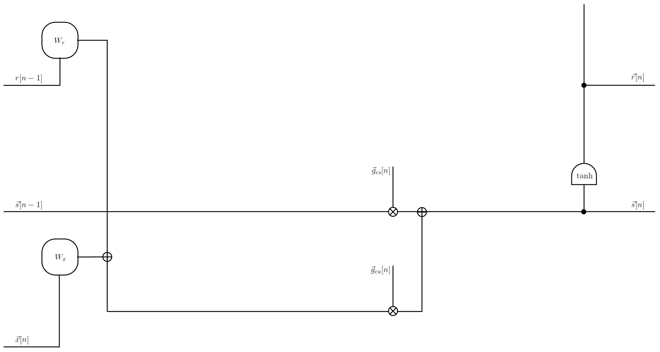
Figure 4: Expanding the canonical RNN system by adding the “control state” gate, $\vec{g}_{cs}[n]$, to control the amount of the state signal, retained from the previous step and the “control update” gate, $\vec{g}_{cu}[n]$, to regulate the amount of the update signal – to be injected into the state signal at the current step.

The elements of gate signals are non-negative fractions. The shorthand notation, $\vec{g}[n]\in[\vec{0},\vec{1}]$ (alternatively, $\vec{0}\leq\vec{g}[n]\leq\vec{1}$), means that the values of all elements of a vector-valued gate signal, $\vec{g}[n]$, at a step with the index, $n$, lie on a closed segment between $0$ and $1$.

The gate signals, $\vec{g}_{cs}[n]$ and $\vec{g}_{cu}[n]$, in Equation 98 and Equation 99 provide a mechanism for exercising a fine-grained control of the two types of contributions to the state signal at every step. Specifically, $\vec{g}_{cs}[n]$ makes it possible to control the amount of the state signal, retained from the previous step, and $\vec{g}_{cu}[n]$ regulates the amount of the update signal – to be injected into the state signal at the current step.

From the derivation of the standard RNN system in Section II, $W_{s}$ in Equation 96 is a diagonal matrix with positive fractions, $\frac{1}{\left|a_{ii}\right|}$, on its main diagonal. Hence, since the elements of $\vec{g}_{cs}[n]$ are also fractions, setting:

$$W_{s} =I$$ (100)

in $\vec{g}_{cs}[n]\odot W_{s}$ is acceptable as long as the gate functions are parametrizable and their parameters are learned during training. Under these conditions, Equation 96 can be simplified to:

$$\vec{\mathcal{F}_{s}}\left(\vec{s}[n-1]\right) =\vec{s}[n-1]$$ (101)

so that Equation 98 becomes:

$$\vec{s}[n] =\vec{g}_{cs}[n]\odot\vec{\mathcal{F}_{s}}\left(\vec{s}[n-1]\right)+\vec{g}_{cu}[n]\odot\vec{\mathcal{F}_{u}}\left(\vec{r}[n-1],\vec{x}[n]\right)$$

$$=\vec{g}_{cs}[n]\odot\vec{s}[n-1]+\vec{g}_{cu}[n]\odot\vec{\mathcal{F}_{u}}\left(\vec{r}[n-1],\vec{x}[n]\right)$$ (102)

Hence, the contribution from the state signal at the previous step remains fractional, insuring the stability of the overall system. Diagrammatically, the insertion of the expanded controls from Equation 102 into the canonical RNN system of Equation 30 transforms Figure 1 into Figure 4.

While the update term, $\vec{\mathcal{F}_{u}}\left(\vec{r}[n-1],\vec{x}[n]\right)$, as a whole is now controlled by $\vec{g}_{cu}[n]$ , the internal composition of $\vec{\mathcal{F}_{u}}\left(\vec{r}[n-1],\vec{x}[n]\right)$ itself needs to be examined. According to Equation 97, the readout signal from the previous step and the input signal at the current step constitute the update candidate signal on every step with the index, $n$, with both of these terms contributing in equal proportions. The issue with always utilizing $W_{r}\vec{r}[n-1]$ in its entirety is that when $\vec{g}_{cu}[n]\sim 1$, $\vec{s}[n-1]$ and $\vec{s}[n]$ become connected through $W_{r}$ and the warping function. Based on Equation 91, this link constrains the gradient of the objective function with respect to the state signal, thus predisposing the system to the vanishing/exploding gradients problem. To throttle this feedback path, the readout signal, $\vec{r}[n]$, will be apportioned by another gate signal, $\vec{g}_{cr}[n]$ (“control readout”), as follows:

$$\vec{v}[n] =\vec{g}_{cr}[n]\odot\vec{r}[n]$$ (103)

$$\vec{0} \leq\vec{g}_{cr}[n]\leq\vec{1}$$ (104)

The gating control, $\vec{g}_{cr}[n]$, determines the fractional amount of the readout signal that becomes the cell’s observable value signal at the step with the index, $n$. Thus, using $\vec{v}[n-1]$ in place of $\vec{r}[n-1]$ in Equation 97 transforms it into:

$$\vec{\mathcal{F}_{u}}\left(\vec{v}[n-1],\vec{x}[n]\right) =W_{r}\vec{v}[n-1]+W_{x}\vec{x}[n]+\vec{\theta}_{s}$$ (105)

The RNN cell schematic diagram, expanded to accommodate the control readout gate, introduced in Equation 103, and the modified recurrence relationship, employed in Equation 105, appears in Figure 5.

Figure 5: The “control readout” gate, $\vec{g}_{cr}[n]$, determines the fractional amount of the readout signal that becomes the cell’s observable value signal at the current step.

Even though the external input does not affect the system’s stability or impact its susceptibility to vanishing/exploding gradients, pairing the input with its own “control input” gate makes the system more flexible.

Multiplying the external input signal, $\vec{x}[n]$, in Equation 97 by a dedicated gate signal, $\vec{g}_{cx}[n]$, turns Equation 105 into:

$$\vec{\mathcal{F}_{u}}\left(\vec{v}[n-1],\vec{x}[n]\right) =W_{r}\vec{v}[n-1]+\vec{g}_{cx}[n]\odot W_{x}\vec{x}[n]+\vec{\theta}_{s}$$ (106)

According to Equation 103 and Equation 106, utilizing both the control readout gate, $\vec{g}_{cr}[n]$, and the control input gate, $\vec{g}_{cx}[n]$, allows for the update term, $\vec{\mathcal{F}_{u}}\left(\vec{v}[n-1],\vec{x}[n]\right)$, to contain an arbitrary mix of the readout signal and the external input. The control input gate signal, $\vec{g}_{cx}[n]$, will be later incorporated as part of extending the Vanilla LSTM cell. For now, it is assumed for simplicity that $\vec{g}_{cx}[n]=\vec{1}$, so Equation 106 reduces to Equation 105.

The dynamic range of the value signal of the cell, $\vec{v}[n]$, is determined by the readout signal, $\vec{r}[n]$, which is bounded by the warping nonlinearity, $G_{d}(z)$. In order to maintain the same dynamic range while absorbing the contributions from the input signal, $\vec{x}[n]$ (or $\vec{g}_{cx}[n]\odot\vec{x}[n]$ if the control input gate is part of the system architecture), the aggregate signal, $\vec{\mathcal{F}_{u}}\left(\vec{v}[n-1],\vec{x}[n]\right)$, is tempered by the saturating warping nonlinearity, $G_{d}(z)$, so as to produce the update candidate signal, $\vec{u}[n]$:

$$\vec{u}[n] =G_{d}\left(\vec{\mathcal{F}_{u}}\left(\vec{v}[n-1],\vec{x}[n]\right)\right)$$ (107)

Thus, replacing the update term in Equation 102 with $\vec{u}[n]$, given by Equation 107, finally yields:

$$\vec{s}[n] =\vec{g}_{cs}[n]\odot\vec{s}[n-1]+\vec{g}_{cu}[n]\odot\vec{u}[n]$$ (108)

which is a core constituent of the set of formulas defining the cell of the Vanilla LSTM network. According to Equation 108, the state signal of the cell at the current step is a weighted combination of the state signal of the cell at the previous step and the aggregation of historical and novel update information available at the present step. The complete data path of the Vanilla LSTM cell, culminating from fortifying the canonical RNN system with gating controls and signal containment, is illustrated in Figure 6.

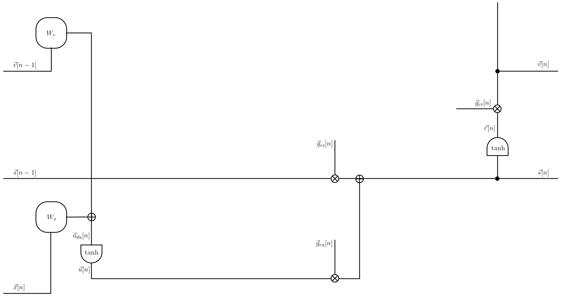
Figure 6: In the Vanilla LSTM network, the state signal of the cell at the current step is a weighted combination of the state signal of the cell at the previous step and the aggregation of historical and novel update information available at the present step.

Example 2.

For an idealized illustration of the ability of the LSTM cell to propagate the error gradient unattenuated, set $\vec{g}_{cs}[n]$ to $\vec{1}$ and both, $\vec{g}_{cu}[n]$ and $\vec{g}_{cr}[n]$, to $\vec{0}$ for all steps in the segment. Then $\vec{s}[n]=\vec{s}[n-1]$ and $\vec{\psi}[n]=\vec{\psi}[n+1]$ for all steps in the segment. The inventors of the LSTM network named this mode the “Constant Error Carousel” (CEC) to underscore that the error gradient is recirculated and the state signal of the cell is refreshed on every step. Essentially, the multiplicative gate units open and close access to constant error gradient flow through CEC as part of the operation of the LSTM cell [21, 12].

In Section IV, we saw that the error gradient determines the parameter updates for training the standard RNN by Gradient Descent. It will become apparent in Section VI-I that the same relationship holds for the Vanilla LSTM network as well. The difference is that because of the gates, the function for the error gradient of the LSTM network accommodates Gradient Descent better than that of the standard RNN does. As will be shown in Section VI-J, under certain provisions regarding the model parameters, the unrolled Vanilla LSTM cell operates in the CEC mode. If such a parameter combination emerges during training, then the parameter update information, embedded in the error gradient signal, will be back-propagated over a large number of steps of a training subsequence, imparting sensitivity to the long-range dependencies to the model parameters through the parameter update step of Gradient Descent. If the training process steers the model parameters toward causing $\left\|\vec{g}_{cs}[n]\right\|=1$ (as in Example 2), then the LSTM network circumvents the vanishing gradient problem in this asymptotic case.

Analogously to the standard RNN, the Vanilla LSTM network, trained by Gradient Descent, can also learn the short-range dependencies among the samples of the subsequences, comprising the training data. Suppose that during training the model parameters cause $\left\|\vec{g}_{cs}[n]\right\|<1$ (unlike in Example 2). Then, as will be elaborated in Section VI-J, the error gradient signal will decline, eventually vanishing over a finite number of steps, even if during training $\left\|\vec{g}_{cu}[n]\right\|>0$ and/or $\left\|\vec{g}_{cr}[n]\right\|>0$ so as to admit (by Equation 108) the contributions from the update candidate signal, $\vec{u}[n]$, into the composition of the state signal.

It remains to define the expressions for the gate signals, $\vec{g}_{cs}[n]$, $\vec{g}_{cr}[n]$, and $\vec{g}_{cu}[n]$. Assuming that the system will be trained with BPTT, all of its constituent functions, including the functions for the gate signals, must be differentiable. A convenient function that is continuous, differentiable, monotonically increasing, and maps the domain $(-\infty,\infty)$ into the range $(0,1)$ is the logistic function:

$$G_{c}(z) \equiv\sigma(z)\equiv\frac{1}{1+e^{-z}}$$ (109)

$$=\frac{1+\tanh(\frac{z}{2})}{2}$$ (110)

$$=\frac{1+G_{d}(\frac{z}{2})}{2}$$ (111)

which is a shifted, scaled, and re-parameterized replica of the hyperbolic tangent, used as the warping function, $G_{d}(z)$, for the data signals in RNN and LSTM systems. When operating on vector arguments, $G_{c}(\vec{z})$ is computed by applying Equation 109 to each element of the vector, $\vec{z}$, separately; the same rule applies to $G_{d}(\vec{z})$.

In order to determine the fractional values of the control signals, $\vec{g}_{cs}[n]$, $\vec{g}_{cu}[n]$, and $\vec{g}_{cr}[n]$, at the step with the index, $n$, all the data signals, from as close as possible to the index of the current step, are utilized. Specifically, for both, $\vec{g}_{cs}[n]$, which determines the fraction of the state signal, $\vec{s}[n-1]$, from the previous step and $\vec{g}_{cu}[n]$, which determines the fraction of the update candidate signal, $\vec{u}[n]$, from the current step, the available data signals are $\vec{s}[n-1]$, $\vec{v}[n-1]$, and $\vec{x}[n]$. However, note that for $\vec{g}_{cr}[n]$, which determines the fraction of the readout signal, $\vec{r}[n]$, from the current step, the available data signals are $\vec{s}[n]$, $\vec{v}[n-1]$, and $\vec{x}[n]$. This is because by Equation 103, $\vec{r}[n]$ is available at the junction of the cell, where $\vec{g}_{cr}[n]$ is computed, and hence, by Equation 95, $\vec{s}[n]$ is necessarily available. The input to each gate is presented as a linear combination of all the data signals available to it:

$$\vec{z}_{cs}[n] =W_{x_{cs}}\vec{x}[n]+W_{s_{cs}}\vec{s}[n-1]+W_{v_{cs}}\vec{v}[n-1]+\vec{\theta}_{cs}$$ (112)

$$\vec{z}_{cu}[n] =W_{x_{cu}}\vec{x}[n]+W_{s_{cu}}\vec{s}[n-1]+W_{v_{cu}}\vec{v}[n-1]+\vec{\theta}_{cu}$$ (113)

$$\vec{z}_{cr}[n] =W_{x_{cr}}\vec{x}[n]+W_{s_{cr}}\vec{s}[n]+W_{v_{cr}}\vec{v}[n-1]+\vec{\theta}_{cr}$$ (114)

Accumulating the available data signals linearly makes the application of the chain rule for BPTT straightforward, while providing a rich representation of the system’s data as an input to each gate at every step. As the model parameters, $\left\{W_{x_{cr}},W_{x_{cu}},W_{x_{cs}},W_{s_{cs}},W_{v_{cs}},\vec{\theta}_{cs},W_{s_{cu}},W_{v_{cu}},\vec{\theta}_{cu},W_{s_{cr}},W_{v_{cr}},\vec{\theta}_{cr}\right\}$, in Equation 112, Equation 113, and Equation 114 are being trained, the gate functions, given by:

$$\vec{g}_{cs}[n] =G_{c}(\vec{z}_{cs}[n])$$ (115)

$$\vec{g}_{cu}[n] =G_{c}(\vec{z}_{cu}[n])$$ (116)

$$\vec{g}_{cr}[n] =G_{c}(\vec{z}_{cr}[n])$$ (117)

become attuned to the flow of and the variations in the training data through the system at every step. During inference, this enables the gates to modulate their corresponding data signals adaptively, utilizing all the available information at every step. In particular, the gates help to detect and mitigate the detrimental ramifications of artificial boundaries, which arise in the input sequences, due to the implicit truncation, caused by unrolling [49, 37, 76]. The gates make the LSTM system a robust model that compensates for the imperfections in the external data and is capable of generating high quality output sequences.

This concludes the derivation of the Vanilla LSTM network. The next section presents a formal self-contained summary of the Vanilla LSTM system, including the equations for training it using BPTT.

VI The Vanilla LSTM Network Mechanism in Detail

VI-A Overview

Suppose that an LSTM cell is unrolled for $K$ steps. The LSTM cell at the step with the index, $n$ (in the sequence of $K$ steps), accepts the input signal, $\vec{x}[n]$, and computes the externally-accessible (i.e., observable) signal, $\vec{v}[n]$. The internal state signal of the cell at the step with the index, $n$, is maintained in $\vec{s}[n]$, which is normally not observable by entities external to the cell. However, the computations, associated with the cell at the next adjacent step in the increasing order of the index, $n$ (i.e., the LSTM step at the index, $n+1$), are allowed to access $\vec{s}[n]$, the state signal of the LSTM cell at the step with the index, $n$.

The key principle of the LSTM cell centers around organizing its internal operations according to two qualitatively different, yet cooperating, objectives: data and the control of data. The data components prepare the candidate data signals (ranging between $-1$ and $1$), while the control components prepare the “throttle” signals (ranging between $0$ and $1$). Multiplying the candidate data signal by the control signal apportions the fractional amount of the candidate data that is allowed to propagate to its intended nodes in the cell. Hence, if the control signal is $0$, then $0\%$ of the candidate data amount will propagate. Conversely, if the control signal is 1, then 10$0\%$ of the candidate data amount will propagate. Analogously, for intermediate values of the control signal (in the range between $0$ and $1$), the corresponding percentage of the candidate data amount will be made available to the next function in the cell.

As depicted in Figure 7, the Vanilla LSTM cell contains three candidate-data/control stages: update, state, and readout.

VI-B Notation

The following notation is used consistently throughout this section to define the Vanilla LSTM cell:

• $n$ – index of a step in the segment (or subsequence); $n=0,\ldots,K-1$

• $K$ – number of steps in the unrolled segment (or subsequence)

• $G_{c}$ – monotonic, bipolarly-saturating warping function for control/throttling purposes (acts as a “gate”)

• $G_{d}$ – monotonic, negative-symmetric, bipolarly-saturating warping function for data bounding purposes

• $d_{x}$ – dimensionality of the input signal to the cell

• $d_{s}$ – dimensionality of the state signal of the cell

• $\vec{x}\in\mathbb{R}^{d_{x}}$ – the input signal to the cell

• $\vec{s}\in\mathbb{R}^{d_{s}}$ – the state signal of the cell

• $\vec{v}\in\mathbb{R}^{d_{s}}$ – the observable value signal of the cell for external purposes (e.g., for connecting one step to the next adjacent step of the same cell in the increasing order of the step index, $n$; as input to another cell in the cascade of cells; for connecting to the signal transformation filter for data output; etc.)

• $\vec{a}\in\mathbb{R}^{d_{s}}$ – an accumulation node of the cell (linearly combines the signals from the preceding step and the present step as net input to a warping function at the present step; each cell contains several purpose-specific control and data accumulation nodes)

• $\vec{u}\in\mathbb{R}^{d_{s}}$ – the update candidate signal for the state signal of the cell

• $\vec{r}\in\mathbb{R}^{d_{s}}$ – the readout candidate signal of the cell

• $g\in\mathbb{R}^{d_{s}}$ – a gate output signal of the cell for control/throttling purposes

• $E\in\mathbb{R}$ – objective (cost) function to be minimized as part of the model training procedure

• $\vec{x}^{T}\vec{v}$ – vector-vector inner product (yields a scalar)

• $\vec{x}\vec{v}^{T}$ – vector-vector outer product (yields a matrix)

• $W\vec{v}$ – matrix-vector product (yields a vector)

• $\vec{x}\odot\vec{v}$ – element-wise vector product (yields a vector)

VI-C Control/Throttling (“Gate”) Nodes

The Vanilla LSTM cell uses three gate types:

• control of the fractional amount of the update candidate signal used to comprise the state signal of the cell at the present step with the index, $n$

• control of the fractional amount of the state signal of the cell at the adjacent lower-indexed step, $n-1$, used to comprise the state signal of the cell at the present step with the index, $n$

• control of the fractional amount of the readout candidate signal used to release as the externally-accessible (observable) signal of the cell at the present step with the index, $n$

VI-D Data Set Standardization

Before the operation of the LSTM network (or its parent, RNN) can commence, the external training data set, $\vec{x}_{0}[n]$, needs to be standardized, such that all elements of the input to the network, $\vec{x}[n]$, have the mean of $0$ and the standard deviation of $1$ over the training set:

$$\vec{\mu} =\frac{1}{N}\sum_{n=0}^{N-1}\vec{x}_{0}[n]$$ (118)

$$\mathsf{\mathcal{V}} =\frac{1}{N-1}\sum_{n=0}^{N-1}\left(\vec{x}_{0}[n]-\vec{\mu}\right)\left(\vec{x}_{0}[n]-\vec{\mu}\right)^{T}$$ (119)

$$\vec{x}[n] =\left[diag\left(\sqrt{\mathcal{V}_{ii}}\right)\right]^{-1}\left(\vec{x}_{0}[n]-\vec{\mu}\right)$$ (120)

Applying the transformations in Equation 118, Equation 119, and Equation 120 to the external training samples, $\vec{x}_{0}[n]$, accomplishes this task. In these equations, $N$ is the number of samples in the training set, $\vec{\mu}$ is the sample mean, and $\mathsf{\mathcal{V}}$ is the sample auto-covariance matrix of the training set.

VI-E Warping (Activation) Functions

As described in Section VI-A, the warping function for control needs to output a value between $0$ and $1$. The sigmoidal (also known as “logistic”) nonlinearity is a good choice, because it is bipolarly-saturating between these values and is monotonic, continuous, and differentiable:

$$G_{c}(z) \equiv\sigma(z)\equiv\frac{1}{1+e^{-z}}=\frac{1+\tanh(\frac{z}{2})}{2}=\frac{1+G_{d}(\frac{z}{2})}{2}$$ (121)

Related to this function, the hyperbolic tangent is a suitable choice for the warping function for data bounding purposes:

$$G_{d}(z) \equiv\tanh(z)=\frac{e^{z}-e^{-z}}{e^{z}+e^{-z}}=2\sigma(2z)-1=2G_{c}(2z)-1$$ (122)

because it is monotonic, negative-symmetric, and bipolarly-saturating at $-1$ and $1$ (i.e., one standard deviation of $\vec{x}[n]$ in each direction). This insures that the data warping function, $G_{d}(z)$, will support both negative and positive values of the standardized incoming data signal, $\vec{x}[n]$, in Equation 120, and keep it bounded within that range (the “squashing” property).

VI-F Vanilla LSTM Cell Model Parameters

The Vanilla LSTM cell model uses the following fifteen (15) parameter entities (with their respective dimensions and
designations as indicated below):

VI-F1 Parameters of the accumulation node, $\vec{a}_{cu}[n]$, of the gate that controls the fractional amount of the update candidate signal, $\vec{u}[n]$, used to comprise the state signal of the cell at the present step with the index, $n$

• $W_{x_{cu}}\in\mathbb{R}^{d_{s}\times d_{x}}$ – the matrix of weights connecting the input signal, $\vec{x}[n]$, at the present step with the index, $n$, to the “control update” accumulation node, $\vec{a}_{cu}[n]$, of the cell at the present step with the index, $n$

• $W_{s_{cu}}\mathbb{\in R}^{d_{s}\times d_{s}}$ – the matrix of weights connecting the state signal, $\vec{s}[n-1]$, at the adjacent lower-indexed step with the index, $n-1$, to the “control update” accumulation node, $\vec{a}_{cu}[n]$, of the cell at the present step with the index, $n$

• $W_{v_{cu}}\mathbb{\in R}^{d_{s}\times d_{s}}$ – the matrix of weights connecting the externally-accessible (observable) value signal, $\vec{v}[n-1]$, at the adjacent lower-indexed step with the index, $n-1$, to the “control update” accumulation node, $\vec{a}_{cu}[n]$, of the cell at the present step with the index, $n$

• $\vec{b}_{cu}\in\mathbb{R}^{d_{s}}$ – the vector of bias elements for the “control update” accumulation node, $\vec{a}_{cu}[n]$, of the cell at the present step with the index, $n$

VI-F2 Parameters of the accumulation node, $\vec{a}_{cs}[n]$, of the gate that controls the fractional amount of the state signal of the cell, $\vec{s}[n-1]$, at the adjacent lower-indexed step, $n-1$, used to comprise the state signal of the cell at the present step with the index, $n$

• $W_{x_{cs}}\in\mathbb{R}^{d_{s}\times d_{x}}$ – the matrix of weights connecting the input signal, $\vec{x}[n]$, at the present step with the index, $n$, to the “control state” accumulation node, $\vec{a}_{cs}[n]$, of the cell at the present step with the index, $n$

• $W_{s_{cs}}\mathbb{\in R}^{d_{s}\times d_{s}}$ – the matrix of weights connecting the state signal, $\vec{s}[n-1]$, at the adjacent lower-indexed step with the index, $n-1$, to the “control state” accumulation node, $\vec{a}_{cs}[n]$, of the cell at the present step with the index, $n$

• $W_{v_{cs}}\mathbb{\in R}^{d_{s}\times d_{s}}$ – the matrix of weights connecting the externally-accessible (observable) value signal, $\vec{v}[n-1]$, at the adjacent lower-indexed step with the index, $n-1$, to the “control state” accumulation node, $\vec{a}_{cs}[n]$, of the cell at the present step with the index, $n$

• $\vec{b}_{cs}\in\mathbb{R}^{d_{s}}$ – the vector of bias elements for the “control state” accumulation node, $\vec{a}_{cs}[n]$, of the cell at the present step with the index, $n$

VI-F3 Parameters of the accumulation node, $\vec{a}_{cr}[n]$, of the gate that controls the fractional amount of the readout candidate signal, $\vec{r}[n]$, used to release as the externally-accessible (observable) value signal of the cell at the present step with the index, $n$

• $W_{x_{cr}}\in\mathbb{R}^{d_{s}\times d_{x}}$ – the matrix of weights connecting the input signal, $\vec{x}[n]$, at the present step with the index, $n$, to the “control readout” accumulation node, $\vec{a}_{cr}[n]$, of the cell at the present step with the index, $n$

• $W_{s_{cr}}\mathbb{\in R}^{d_{s}\times d_{s}}$ – the matrix of weights connecting the state signal, $\vec{s}[n]$, at the present step with the index, $n$, to the “control readout” accumulation node, $\vec{a}_{cr}[n]$, of the cell at the present step with the index, $n$

• $W_{v_{cr}}\mathbb{\in R}^{d_{s}\times d_{s}}$ – the matrix of weights connecting the externally-accessible (observable) value signal, $\vec{v}[n-1]$, at the adjacent lower-indexed step with the index, $n-1$, to the “control readout” accumulation node, $\vec{a}_{cr}[n]$, of the cell at the present step with the index, $n$

• $\vec{b}_{cr}\in\mathbb{R}^{d_{s}}$ – the vector of bias elements for the “control readout” accumulation node, $\vec{a}_{cr}[n]$, of the cell at the present step with the index, $n$

VI-F4 Parameters of the accumulation node, $\vec{a}_{du}[n]$, for the data warping function that produces the update candidate signal, $\vec{u}[n]$, of the cell at the present step with the index, $n$

• $W_{x_{du}}\in\mathbb{R}^{d_{s}\times d_{x}}$ – the matrix of weights connecting the input signal, $\vec{x}[n]$, at the present step with the index, $n$, to the “data update” accumulation node, $\vec{a}_{du}[n]$, of the cell at the present step with the index, $n$

• $W_{v_{du}}\mathbb{\in R}^{d_{s}\times d_{s}}$ – the matrix of weights connecting the externally-accessible (observable) value signal, $\vec{v}[n-1]$, at the adjacent lower-indexed step with the index, $n-1$, to the “data update” accumulation node, $\vec{a}_{du}[n]$, of the cell at the present step with the index, $n$

• $\vec{b}_{du}\in\mathbb{R}^{d_{s}}$ – the vector of bias elements for the “data update” accumulation node, $\vec{a}_{du}[n]$, of the cell at the present step with the index, $n$

VI-F5 All model parameters, which must be learned, combined (for notational convenience)

• All parameters of the LSTM network are commonly concatenated and represented as a whole by $\Theta$:

  $$\Theta \equiv\left\{W_{x_{cu}},W_{s_{cu}},W_{v_{cu}},\vec{b}_{cu},W_{x_{cs}},W_{s_{cs}},W_{v_{cs}},\vec{b}_{cs},W_{x_{cr}},W_{s_{cr}},W_{v_{cr}},\vec{b}_{cr}W_{x_{du}},W_{v_{du}},\vec{b}_{du}\right\}$$ (123)

• Arranged “thematically” (attributed by the type of an accumulation), $\Theta$ can be written as:

  $$\begin{gathered}\Theta\equiv\end{gathered} \begin{Bmatrix}W_{x_{cu}},&W_{s_{cu}},&W_{v_{cu}},&\vec{b}_{cu},\\ W_{x_{cs}},&W_{s_{cs}},&W_{v_{cs}},&\vec{b}_{cs},\\ W_{x_{cr}},&W_{s_{cr}},&W_{v_{cr}},&\vec{b}_{cr},\\ W_{x_{du}},&&W_{v_{du}},&\vec{b}_{du}\end{Bmatrix}.$$ (125)

VI-G Summary of the main entities (generalized)

The following glossary lists the main entities of the model in a generalized way (i.e., without the subscripts, indices, etc.). Note that the special quantities $\vec{\psi,}\vec{\chi},\vec{\alpha},\vec{\rho},\vec{\gamma}$ will be defined in Section VI-I.

$$\begin{rcases}\vec{x}\in\mathbb{R}^{d_{x}}\\ \vec{s},\vec{v},\vec{a},\vec{u},\vec{r},\vec{g}\in\mathbb{R}^{d_{s}}\\ \vec{\psi},\vec{\chi},\vec{\alpha},\vec{\rho},\vec{\gamma}\in\mathbb{R}^{d_{s}}\\ W_{x}\in\mathbb{R}^{d_{s}\times d_{x}}\\ W_{s},W_{v}\in\mathbb{R}^{d_{s}\times d_{s}}\\ \vec{b}\in\mathbb{R}^{d_{s}}\\ E\\ N\\ K\\ n=0,\ldots,K-1\end{rcases}$$ (126)

VI-H Vanilla LSTM System Equations (“Forward Pass”)

It is important to highlight the general pattern of computations that govern the processes, according to which any RNN cell, and the LSTM network cell in particular, unrolled for $K$ steps, generates sequences of samples. Namely, the quantities that characterize the step of the cell at the index, $n$, of the sequence depend on the quantities that characterize the step of the cell at the index, $n-1$, of the sequence. The following equations fully define the Vanilla LSTM cell:

$$\vec{a}_{cu}[n] =W_{x_{cu}}\vec{x}[n]+W_{s_{cu}}\vec{s}[n-1]+W_{v_{cu}}\vec{v}[n-1]+\vec{b}_{cu}$$ (127)

$$\vec{a}_{cs}[n] =W_{x_{cs}}\vec{x}[n]+W_{s_{cs}}\vec{s}[n-1]+W_{v_{cs}}\vec{v}[n-1]+\vec{b}_{cs}$$ (128)

$$\vec{a}_{cr}[n] =W_{x_{cr}}\vec{x}[n]+W_{s_{cr}}\vec{s}[n]+W_{v_{cr}}\vec{v}[n-1]+\vec{b}_{cr}$$ (129)

$$\vec{a}_{du}[n] =W_{x_{du}}\vec{x}[n]+W_{v_{du}}\vec{v}[n-1]+\vec{b}_{du}$$ (130)

$$\vec{u}[n] =G_{d}(\vec{a}_{du}[n])$$ (131)

$$\vec{g}_{cu}[n] =G_{c}(\vec{a}_{cu}[n])$$ (132)

$$\vec{g}_{cs}[n] =G_{c}(\vec{a}_{cs}[n])$$ (133)

$$\vec{g}_{cr}[n] =G_{c}(\vec{a}_{cr}[n])$$ (134)

$$\vec{s}[n] =\vec{g}_{cs}[n]\odot\vec{s}[n-1]+\vec{g}_{cu}[n]\odot\vec{u}[n]$$ (135)

$$\vec{r}[n] =G_{d}(\vec{s}[n])$$ (136)

$$\vec{v}[n] =\vec{g}_{cr}[n]\odot\vec{r}[n]$$ (137)

The schematic diagram of the Vanilla LSTM cell, defined by Equations 127 – 137, is presented in Figure 7, and the snapshot of unrolling it (for only $4$ steps as an illustration) appears in Figure 8. In order to make it easier to isolate the specific functions performed by the components of the Vanilla LSTM cell, its schematic diagram is redrawn in Figure 9, with the major stages comprising the cell’s architecture marked by dashed rectangles annotated by the names of the respective enclosed stages.

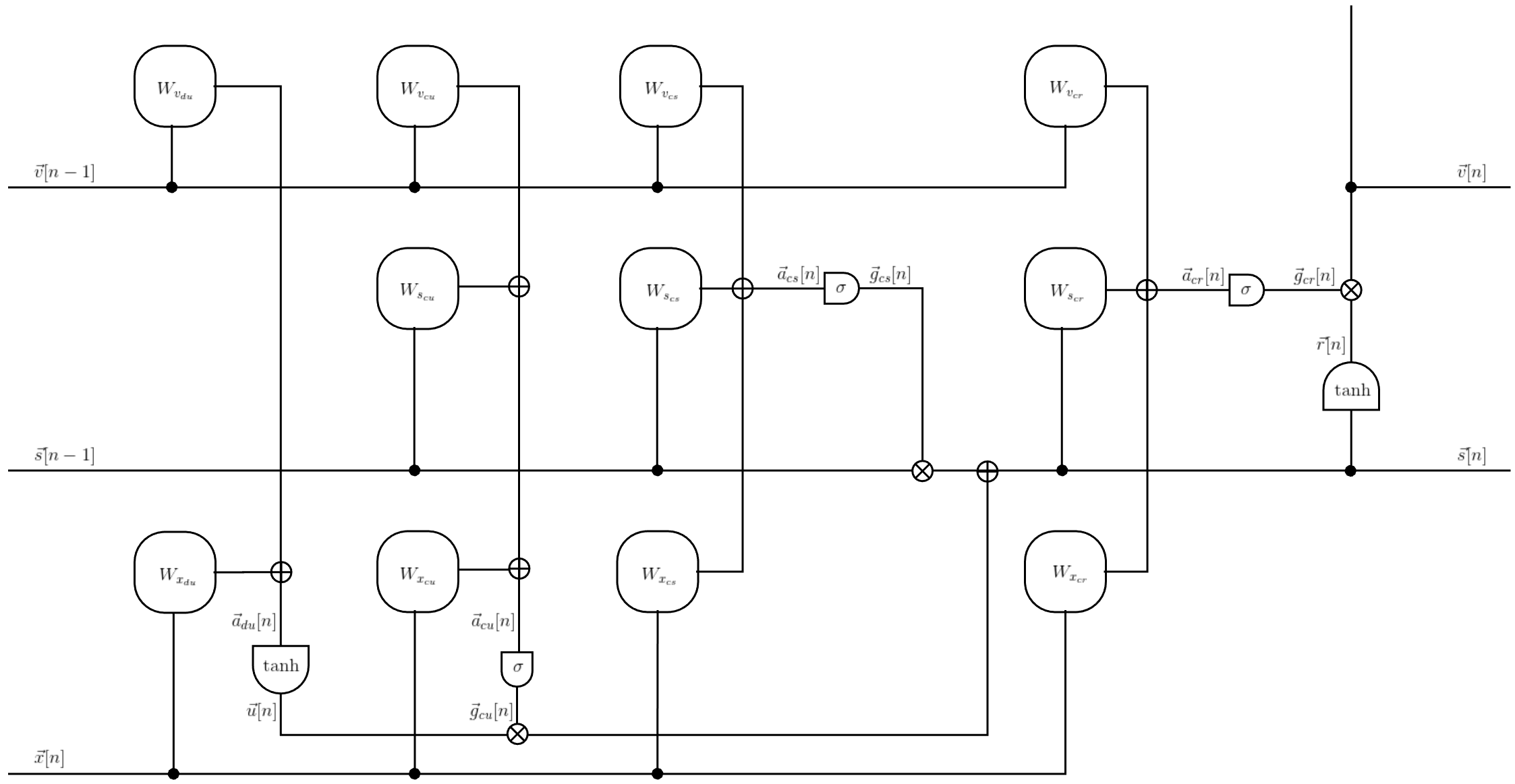
Figure 7: Vanilla LSTM network cell. The bias parameters, $\vec{b},$ have been omitted from the figure for brevity. They can be assumed to be included without the loss of generality by appending an additional element, always set to $1$, to the input signal vector, $\vec{x}[n]$, and increasing the row dimensions of all corresponding weight matrices by $1$.

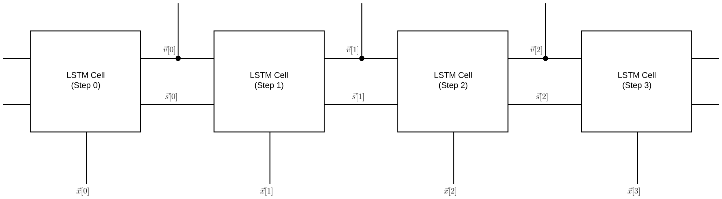
Figure 8: Sequence of steps generated by unrolling a cell of the LSTM network (displaying $4$ steps for illustration).

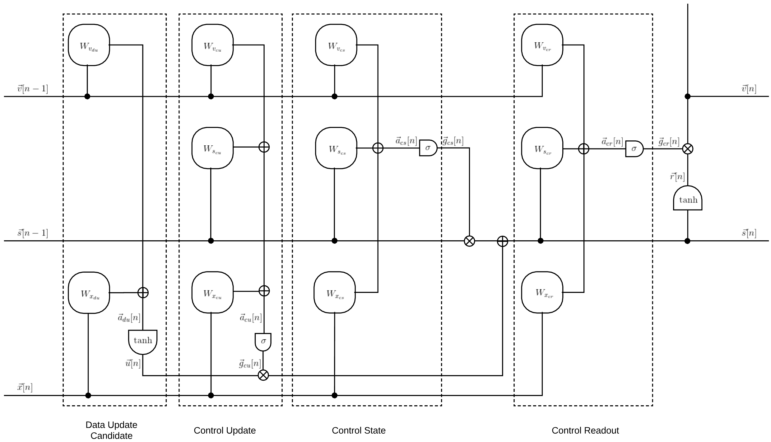
Figure 9: Vanilla LSTM network cell from Figure 7, with the stages of the system delineated by dashed rectangles and annotations that depict the function of each stage. As before, the bias parameters, $\vec{b},$ have been omitted from the figure for brevity. (They can be assumed to be included without the loss of generality by appending an additional element, always set to $1$, to the input signal vector, $\vec{x}[n]$, and increasing the row dimensions of all corresponding weight matrices by $1$.)

VI-I Vanilla LSTM System Derivatives (“Backward Pass”)

This section derives the equations that are necessary for training the Vanilla LSTM network cell, unrolled for $K$ steps, using Back Propagation Through Time (BPTT). To obtain the update equations for the parameters of the system, two auxiliary “backward-moving” gradient sequences, indexed by $n$, are computed first: $\vec{\chi}[n]$, the total partial derivative of the objective function, $E$, with respect to the externally-accessible (observable) value signal, $\vec{v}[n]$, and $\vec{\psi}[n]$, the total partial derivative of the objective function, $E$, with respect to the state signal, $\vec{s}[n]$. The decision to “anchor” the chain rule at the border of the cell is made judiciously, guided by the principles of modular design. Expressing every intra-cell total partial derivative in terms of $\vec{\chi}[n]$ (instead of explicitly computing the total partial derivative of the objective function, $E$, with respect to each variable of the cell [42]) reduces the number of intermediate variables. This makes the equations for the backward pass straightforward and a natural fit for an implementation as a pluggable module [74, 73, 15].

Due to the backward-moving recursion of $\vec{\chi}[n]$ and $\vec{\psi}[n]$ (the gradient sequences propagate in the direction opposite to that of the state signal, $\vec{s}[n]$, as a function of the step index, $n$), the values of $\vec{\chi}[n]$ and $\vec{\psi}[n]$ at the index, $n$, depend on the values of the same quantities at the index, $n+1$, subject to the initial conditions. Once $\vec{\chi}[n]$ and $\vec{\psi}[n]$ are known, they are used to compute the total partial derivatives of the objective function, $E$, with respect to the accumulation nodes for each value of the index, $n$. These intermediate gradient sequences, named $\vec{\alpha}_{cs}[n]$, $\vec{\alpha}_{cu}[n]$, $\vec{\alpha}_{cr}[n]$, and $\vec{\alpha}_{du}[n]$, allocate the amounts contributed by the signals associated with the step at the index, $n$, to the total partial derivatives of the objective function, $E$, with respect to the model parameters. By the definition of the total derivative, these contributions have to be summed across all steps, $0\leq n\leq K-1$, to produce the total partial derivatives of the objective function, $E$, with respect to the model parameters.

During the inference phase of the LSTM system, only $\vec{x}[n]$ (the input signal) and $\vec{v}[n]$ (the value signal) are externally accessible (i.e., observable). The cell accepts the input signal at each step and computes the value signal for all steps. All the other intermediate signals are available only to the internal components and nodes of the cell, with the exception of $\vec{s}[n]$ (state signal) and $\vec{v}[n]$ (value signal), which serve both the inter- and the intra-step purposes throughout the unrolled sequence.

The cell’s value signal, $\vec{v}[n]$, at the step with the index, $n$, can be further transformed to produce the output signal, $\vec{y}[n]$ (e.g., a commonly used form of $\vec{y}[n]$ may be obtained by computing a linear transformation of $\vec{v}[n]$, followed by a softmax operator, or a different decision function). Likewise, the input signal, too, may result from the transformation of the original raw data. For example, one kind of input pre-processing can convert the vocabulary “one-hot” vector into a more compact representation. Also, for applications where the input data set can be collected for the entire segment at once, input samples that lie within a small window surrounding the given step can be combined so as to enhance the system’s “attention” to context. A non-causal input filter, designed for this purpose, will be introduced in Section VII-A as part of extending the Vanilla LSTM cell.

We start by computing the derivatives of the warping functions from their definitions in Equation 121 and Equation 122, respectively:

$$\frac{dG_{c}(z)}{dz} =G_{c}(z)(1-G_{c}(z))$$ (138)

$$\frac{dG_{d}(z)}{dz} =1-(G_{d}(z))^{2}$$ (139)

Next, we anchor the chain rule at the border of the cell by defining $\vec{\chi}[n]$ as the total partial derivative of the objective function, $E$, with respect to the externally-accessible (observable) value signal, $\vec{v}[n]$, as follows:

$$\vec{\chi}[n] \equiv\vec{\nabla}_{\vec{v}[n]}E=\frac{\partial E}{\partial\vec{v}[n]}$$ (140)

As will become imminently evident, having $\vec{\chi}[n]$ not only makes training equations for the Vanilla LSTM cell amenable for a modular implementation at the step level, but also greatly simplifies them.

We also define the total partial derivatives of the objective function, $E$, with respect to three intermediate (i.e., away from the border) variables and another border variable of the Vanilla LSTM cell:

$$\vec{\rho}[n] \equiv\vec{\nabla}_{\vec{r}[n]}E=\frac{\partial E}{\partial\vec{r}[n]}$$ (141)

$$\vec{\gamma}[n] \equiv\vec{\nabla}_{\vec{g}[n]}E=\frac{\partial E}{\partial\vec{g}[n]}$$ (142)

$$\vec{\alpha}[n] \equiv\vec{\nabla}_{\vec{a}[n]}E=\frac{\partial E}{\partial\vec{a}[n]}$$ (143)

$$\vec{\psi}[n] \equiv\vec{\nabla}_{\vec{s}[n]}E=\frac{\partial E}{\partial\vec{s}[n]}$$ (144)

The border quantity in Equation 144, $\vec{\psi}[n]$, is of special significance as it is the total partial derivative of the objective function, $E$, with respect to the state signal, $\vec{s}[n]$, at the index, $n$, of the Vanilla LSTM cell. As in the standard RNN, all parameter updates in the Vanilla LSTM network depend on $\vec{\psi}[n]$, making it the most important error gradient sequence of the system.

The backward pass equations are obtained by utilizing these border and intermediate derivatives in the application of the chain rule to the Vanilla LSTM cell, defined by Equations 127 – 137:

$$\vec{\chi}[n] =\left(\frac{\partial\vec{y}[n]}{\partial\vec{v}[n]}\right)^{T}\left(\frac{\partial E}{\partial\vec{y}[n]}\right)+\vec{f_{\chi}}[n+1]$$ (145)

$$\vec{\rho}[n] =\left(\frac{\partial\vec{v}[n]}{\partial\vec{r}[n]}\right)^{T}\left(\frac{\partial E}{\partial\vec{v}[n]}\right)=\vec{(\nabla}_{\vec{v}[n]}E)\odot\vec{g}_{cr}[n]=\vec{\chi}[n]\odot\vec{g}_{cr}[n]$$ (146)

$$\vec{\gamma}_{cr}[n] =\frac{\partial E}{\partial\vec{v}[n]}\frac{\partial\vec{v}[n]}{\partial\vec{g}_{cr}[n]}=\vec{(\nabla}_{\vec{v}[n]}E)\odot\vec{r}[n]=\vec{\chi}[n]\odot\vec{r}[n]$$ (147)

$$\vec{\alpha}_{cr}[n] =\vec{\gamma}_{cr}[n]\odot\frac{\partial\vec{g}_{cr}[n]}{\partial\vec{a}_{cr}[n]}=\vec{\gamma}_{cr}[n]\odot\frac{dG_{c}(z)}{dz}\rfloor_{z=\vec{a}_{cr}[n]}=\vec{\chi}[n]\odot\vec{r}[n]\odot\frac{dG_{c}(z)}{dz}\rfloor_{z=\vec{a}_{cr}[n]}$$ (148)

$$\vec{\psi}[n] =\vec{\rho}[n]\odot\frac{\partial\vec{r}[n]}{\partial\vec{s}[n]}+\frac{\partial\vec{a}_{cr}[n]}{\partial\vec{s}[n]}\vec{\alpha}_{cr}[n]+\vec{f_{\psi}}[n+1]$$ (149)

$$=\vec{\rho}[n]\odot\frac{dG_{d}(\vec{z})}{d\vec{z}}\rfloor_{z=\vec{s}[n]}+W_{s_{cr}}\vec{\alpha}_{cr}[n]+\vec{f_{\psi}}[n+1]$$ (150)

$$=\vec{\chi}[n]\odot\vec{g}_{cr}[n]\odot\frac{dG_{d}(\vec{z})}{d\vec{z}}\rfloor_{z=\vec{s}[n]}+W_{s_{cr}}\vec{\alpha}_{cr}[n]+\vec{f_{\psi}}[n+1]$$ (151)

$$\vec{\alpha}_{cs}[n] =\vec{\psi}[n]\odot\frac{\partial\vec{s}[n]}{\partial\vec{g}_{cs}[n]}\odot\frac{\partial\vec{g}_{cs}[n]}{\partial\vec{a}_{cs}[n]}=\vec{\psi}[n]\odot\vec{s}[n-1]\odot\frac{dG_{c}(\vec{z})}{d\vec{z}}\rfloor_{z=\vec{a}_{cs}[n]}$$ (152)

$$\vec{\alpha}_{cu}[n] =\vec{\psi}[n]\odot\frac{\partial\vec{s}[n]}{\partial\vec{g}_{cu}[n]}\odot\frac{\partial\vec{g}_{cu}[n]}{\partial\vec{a}_{cu}[n]}=\vec{\psi}[n]\odot\vec{u}[n]\odot\frac{dG_{c}(\vec{z})}{d\vec{z}}\rfloor_{z=\vec{a}_{cu}[n]}$$ (153)

$$\vec{\alpha}_{du}[n] =\vec{\psi}[n]\odot\frac{\partial\vec{s}[n]}{\partial\vec{u}[n]}\odot\frac{dG_{d}(\vec{z})}{d\vec{z}}\rfloor_{z=\vec{a}_{du}[n]}=\vec{\psi}[n]\odot\vec{g}_{cu}[n]\odot\frac{dG_{d}(\vec{z})}{d\vec{z}}\rfloor_{z=\vec{a}_{du}[n]}$$ (154)

where:

$$\vec{f_{\chi}}[n+1] =W_{v_{cu}}^{T}\vec{\alpha}_{cu}[n+1]+W_{v_{cs}}^{T}\vec{\alpha}_{cs}[n+1]+W_{v_{cr}}^{T}\vec{\alpha}_{cr}[n+1]+W_{v_{du}}^{T}\vec{\alpha}_{du}[n+1]$$ (155)

$$\vec{f_{\psi}}[n+1] =W_{s_{cu}}^{T}\vec{\alpha}_{cu}[n+1]+W_{s_{cs}}^{T}\vec{\alpha}_{cs}[n+1]+\vec{g}_{cs}[n+1]\odot\vec{\psi}[n+1]$$ (156)

are the portions of the total derivative of the objective function, $E$, with respect to the cell’s value signal and the cell’s state signal, respectively, contributed by the quantities evaluated at the step with the index, $n+1$.

The total partial derivatives of the objective function, $E$, with respect to the model parameters at the step with the index, $n$, are directly proportional to the “accumulation derivatives”, given by Equation 148, Equation 152, Equation 153, and

Equation 154. Hence, by referring once again to the definition of the Vanilla LSTM cell in Equations 127 – 137, we obtain:

$$\frac{\partial E}{\partial W_{x_{cu}}}[n] =\vec{\alpha}_{cu}[n]\vec{x}^{T}[n]$$ (157)

$$\frac{\partial E}{\partial W_{s_{cu}}}[n] =\vec{\alpha}_{cu}[n]\vec{s}^{T}[n-1]$$ (158)

$$\frac{\partial E}{\partial W_{v_{cu}}}[n] =\vec{\alpha}_{cu}[n]\vec{v}^{T}[n-1]$$ (159)

$$\frac{\partial E}{\partial\vec{b}_{cu}}[n] =\vec{\alpha}_{cu}[n]$$ (160)

$$\frac{\partial E}{\partial W_{x_{cs}}}[n] =\vec{\alpha}_{cs}[n]\vec{x}^{T}[n]$$ (161)

$$\frac{\partial E}{\partial W_{s_{cs}}}[n] =\vec{\alpha}_{cs}[n]\vec{s}^{T}[n-1]$$ (162)

$$\frac{\partial E}{\partial W_{v_{cs}}}[n] =\vec{\alpha}_{cs}[n]\vec{v}^{T}[n-1]$$ (163)

$$\frac{\partial E}{\partial\vec{b}_{cs}}[n] =\vec{\alpha}_{cs}[n]$$ (164)

$$\frac{\partial E}{\partial W_{x_{cr}}}[n] =\vec{\alpha}_{cr}[n]\vec{x}^{T}[n]$$ (165)

$$\frac{\partial E}{\partial W_{s_{cr}}}[n] =\vec{\alpha}_{cr}[n]\vec{s}^{T}[n]$$ (166)

$$\frac{\partial E}{\partial W_{v_{cr}}}[n] =\vec{\alpha}_{cr}[n]\vec{v}^{T}[n-1]$$ (167)

$$\frac{\partial E}{\partial\vec{b}_{cr}}[n] =\vec{\alpha}_{cr}[n]$$ (168)

$$\frac{\partial E}{\partial W_{x_{du}}}[n] =\vec{\alpha}_{du}[n]\vec{x}^{T}[n]$$ (169)

$$\frac{\partial E}{\partial W_{v_{du}}}[n] =\vec{\alpha}_{du}[n]\vec{v}^{T}[n-1]$$ (170)

$$\frac{\partial E}{\partial\vec{b}_{du}}[n] =\vec{\alpha}_{du}[n]$$ (171)

Arranged congruently with Equation 125, the total partial derivative of the objective function, $E$, with respect to the model parameters, $\Theta$, at the step with the index, $n$, is:

$$\begin{gathered}\frac{\partial E}{\partial\Theta}[n]=\end{gathered} \begin{Bmatrix}\frac{\partial E}{\partial W_{x_{cu}}}[n],&\frac{\partial E}{\partial W_{s_{cu}}}[n],&\frac{\partial E}{\partial W_{v_{cu}}}[n],&\frac{\partial E}{\partial\vec{b}_{cu}}[n],\\ \frac{\partial E}{\partial W_{x_{cs}}}[n],&\frac{\partial E}{\partial W_{s_{cs}}}[n],&\frac{\partial E}{\partial W_{v_{cs}}}[n],&\frac{\partial E}{\partial\vec{b}_{cs}}[n],\\ \frac{\partial E}{\partial W_{x_{cr}}}[n],&\frac{\partial E}{\partial W_{s_{cr}}}[n],&\frac{\partial E}{\partial W_{v_{cr}}}[n],&\frac{\partial E}{\partial\vec{b}_{cr}}[n],\\ \frac{\partial E}{\partial W_{x_{du}}}[n],&&\frac{\partial E}{\partial W_{v_{du}}}[n],&\frac{\partial E}{\partial\vec{b}_{du}}[n]\end{Bmatrix}.$$ (173)

When the Vanilla LSTM cell is unrolled for $K$ steps in order to cover one full segment of training samples, the same set of the model parameters, $\Theta$, is shared by all the steps. This is because $\Theta$ is the parameter of the Vanilla LSTM cell as a whole. Consequently, the total derivative of the objective function, $E$, with respect to the model parameters, $\Theta$, has to include the contributions from all steps of the unrolled sequence:

$$\frac{dE}{d\Theta} =\sum_{n=0}^{K-1}\frac{\partial E}{\partial\Theta}[n]$$ (174)

The result from Equation 174 can now be used as part of optimization by Gradient Descent. In practice, Equation 174 is computed for a batch of segments, and the sum of the parameter gradients over all segments in the batch is then supplied to the Gradient Descent algorithm for updating the model parameters.

VI-J Error Gradient Sequences in Vanilla LSTM System

Section V mentions that because of the action of the gates, the LSTM network is more compatible with the Gradient Descent training procedure than the standard RNN system is. As discussed in Section IV and Section VI-I, for Gradient Descent to be effective, the elements of $\frac{\partial E}{\partial\Theta}[n]$ in Equation 173 must be well-behaved numerically. In particular, this implies that the intermediate gradient sequences, $\vec{\alpha}_{cs}[n]$, $\vec{\alpha}_{cu}[n]$, $\vec{\alpha}_{cr}[n]$, and $\vec{\alpha}_{du}[n]$, and hence the border gradient sequences, $\vec{\chi}[n]$ and $\vec{\psi}[n]$, must be able to sustain a steady flow of information over long ranges of the step index, $n$. Expanding Equation 151 produces:

$$\vec{\psi}[n] =\vec{\chi}[n]\odot\vec{g}_{cr}[n]\odot\frac{dG_{d}(\vec{z})}{d\vec{z}}\rfloor_{z=\vec{s}[n]}+W_{s_{cr}}\vec{\chi}[n]\odot\vec{r}[n]\odot\frac{dG_{c}(z)}{dz}\rfloor_{z=\vec{a}_{cr}[n]}+\vec{f_{\psi}}[n+1]$$ (175)

$$=\left(\left(\frac{\partial\vec{y}[n]}{\partial\vec{v}[n]}\right)^{T}\left(\frac{\partial E}{\partial\vec{y}[n]}\right)+\vec{f_{\chi}}[n+1]\right)\odot\vec{g}_{cr}[n]\odot\frac{dG_{d}(\vec{z})}{d\vec{z}}\rfloor_{z=\vec{s}[n]}$$

$$+W_{s_{cr}}\left(\left(\frac{\partial\vec{y}[n]}{\partial\vec{v}[n]}\right)^{T}\left(\frac{\partial E}{\partial\vec{y}[n]}\right)+\vec{f_{\chi}}[n+1]\right)\odot\vec{r}[n]\odot\frac{dG_{c}(z)}{dz}\rfloor_{z=\vec{a}_{cr}[n]}+\vec{f_{\psi}}[n+1]$$ (176)

According to Equation 155 and Equation 156, both $\vec{\chi}[n]$ and $\vec{\psi}[n]$ depend on $\vec{\psi}[n+1]$. Hence, we can follow the approach in Section IV to analyze the dependence of $\vec{\psi}[n]$ on $\left\langle\vec{\psi}[k]\right\rangle\left\rfloor{}_{n<k\leq K-1}\right.$ in order to gauge the sensitivity of the LSTM system to factors conducive to gradient decay. Applying the change of indices, $n\longrightarrow k-1$, and the chain rule to Equation 176 yields:

$$\frac{\partial\vec{\psi}[k-1]}{\partial\vec{\psi}[k]} =\left(\frac{\partial\vec{\psi}[k-1]}{\partial\vec{f_{\chi}}[k]}\right)\left(\frac{\partial\vec{f_{\chi}}[k]}{\partial\vec{\psi}[k]}\right)+\left(\frac{\partial\vec{\psi}[k-1]}{\partial\vec{f_{\psi}}[k]}\right)\left(\frac{\partial\vec{f_{\psi}}[k]}{\partial\vec{\psi}[k]}\right)$$ (177)

$$= \left(\frac{\partial\vec{\psi}[k-1]}{\partial\vec{f_{\chi}}[k]}\right)\left\{\left(\frac{\partial\vec{f_{\chi}}[k]}{\partial\vec{\alpha}_{cu}[k]}\right)\left(\frac{\partial\vec{\alpha}_{cu}[k]}{\partial\vec{\psi}[k]}\right)+\left(\frac{\partial\vec{f_{\chi}}[k]}{\partial\vec{\alpha}_{cs}[k]}\right)\left(\frac{\partial\vec{\alpha}_{cs}[k]}{\partial\vec{\psi}[k]}\right)\right.$$

$$\left.+\left(\frac{\partial\vec{f_{\chi}}[k]}{\partial\vec{\alpha}_{du}[k]}\right)\left(\frac{\partial\vec{\alpha}_{du}[k]}{\partial\vec{\psi}[k]}\right)\right\}+\left(\frac{\partial\vec{\psi}[k-1]}{\partial\vec{f_{\psi}}[k]}\right)\left\{\left(\frac{\partial\vec{f_{\psi}}[k]}{\partial\vec{\alpha}_{cu}[k]}\right)\left(\frac{\partial\vec{\alpha}_{cu}[k]}{\partial\vec{\psi}[k]}\right)\right.$$

$$\left.+\left(\frac{\partial\vec{f_{\psi}}[k]}{\partial\vec{\alpha}_{cs}[k]}\right)\left(\frac{\partial\vec{\alpha}_{cs}[k]}{\partial\vec{\psi}[k]}\right)+\mathit{\mathrm{diag}}\bigg{[}\vec{g}_{cs}[k]\bigg{]}\right\}$$ (178)

$$=\left(\mathrm{diag}\left[\vec{g}_{cr}[k-1]\odot\frac{dG_{d}(\vec{z})}{d\vec{z}}\rfloor_{z=\vec{s}[k-1]}\right]+W_{s_{cr}}\mathrm{diag}\left[\vec{r}[k-1]\odot\frac{dG_{c}(z)}{dz}\rfloor_{z=\vec{a}_{cr}[k-1]}\right]\right)$$

$$\times\left\{W_{v_{cu}}\mathit{\mathrm{diag}}\left[\vec{u}[k]\odot\frac{dG_{c}(\vec{z})}{d\vec{z}}\rfloor_{z=\vec{a}_{cu}[k]}\right]+W_{v_{cs}}\mathit{\mathrm{diag}}\left[\vec{s}[k-1]\odot\frac{dG_{c}(\vec{z})}{d\vec{z}}\rfloor_{z=\vec{a}_{cs}[k]}\right]\right.$$

$$\left.+W_{v_{du}}\mathit{\mathrm{diag}}\left[\vec{g}_{cu}[k]\odot\frac{dG_{d}(\vec{z})}{d\vec{z}}\rfloor_{z=\vec{a}_{du}[k]}\right]\right\}+\left(W_{s_{cu}}\mathit{\mathrm{diag}}\left[\vec{u}[k]\odot\frac{dG_{c}(\vec{z})}{d\vec{z}}\rfloor_{z=\vec{a}_{cu}[k]}\right]\right.$$

$$\left.+W_{s_{cs}}\mathit{\mathrm{diag}}\left[\vec{s}[k-1]\odot\frac{dG_{c}(\vec{z})}{d\vec{z}}\rfloor_{z=\vec{a}_{cs}[k]}\right]+\mathit{\mathrm{diag}}\bigg{[}\vec{g}_{cs}[k]\bigg{]}\right)$$ (179)

$$=\mathit{\mathrm{diag}}\left[\vec{u}[k]\odot\frac{dG_{c}(\vec{z})}{d\vec{z}}\rfloor_{z=\vec{a}_{cu}[k]}\right]$$

$$\times\left\{W_{v_{cu}}\left(\mathrm{diag}\left[\vec{g}_{cr}[k-1]\odot\frac{dG_{d}(\vec{z})}{d\vec{z}}\rfloor_{z=\vec{s}[k-1]}\right]+W_{s_{cr}}\mathrm{diag}\left[\vec{r}[k-1]\odot\frac{dG_{c}(z)}{dz}\rfloor_{z=\vec{a}_{cr}[k-1]}\right]\right)+W_{s_{cu}}\right\}$$

$$+\mathit{\mathrm{diag}}\left[\vec{s}[k-1]\odot\frac{dG_{c}(\vec{z})}{d\vec{z}}\rfloor_{z=\vec{a}_{cs}[k]}\right]$$

$$\times\left\{W_{v_{cs}}\left(\mathrm{diag}\left[\vec{g}_{cr}[k-1]\odot\frac{dG_{d}(\vec{z})}{d\vec{z}}\rfloor_{z=\vec{s}[k-1]}\right]+W_{s_{cr}}\mathrm{diag}\left[\vec{r}[k-1]\odot\frac{dG_{c}(z)}{dz}\rfloor_{z=\vec{a}_{cr}[k-1]}\right]\right)+W_{s_{cs}}\right\}$$

$$+\mathit{\mathrm{diag}}\left[\vec{g}_{cu}[k]\odot\frac{dG_{d}(\vec{z})}{d\vec{z}}\rfloor_{z=\vec{a}_{du}[k]}\right]$$

$$\times\left\{W_{v_{du}}\left(\mathrm{diag}\left[\vec{g}_{cr}[k-1]\odot\frac{dG_{d}(\vec{z})}{d\vec{z}}\rfloor_{z=\vec{s}[k-1]}\right]+W_{s_{cr}}\mathrm{diag}\left[\vec{r}[k-1]\odot\frac{dG_{c}(z)}{dz}\rfloor_{z=\vec{a}_{cr}[k-1]}\right]\right)\right\}+\mathit{\mathrm{diag}}\bigg{[}\vec{g}_{cs}[k]\bigg{]}$$ (180)

$$=Q\left(k-1,k;\tilde{\Theta}\right)+\mathit{\mathrm{diag}}\bigg{[}\vec{g}_{cs}[k]\bigg{]}$$ (181)

where $\tilde{\Theta}=\left\{W_{s_{cu}},W_{v_{cu}},W_{s_{cs}},W_{v_{cs}},W_{s_{cr}},W_{v_{du}}\right\}$, and $Q\left(k-1,k;\tilde{\Theta}\right)$ subsumes all the terms in $\frac{\partial\vec{\psi}[k-1]}{\partial\vec{\psi}[k]}$, excluding $\mathit{\mathrm{diag}}\bigg{[}\vec{g}_{cs}[k]\bigg{]}$.

Extrapolating $\frac{\partial\vec{\psi}[k-1]}{\partial\vec{\psi}[k]}$ from the step with the index, $n,$ to the step with the index, $l\leq K-1$, where $l\gg n$, gives:

$$\frac{\partial\vec{\psi}[n]}{\partial\vec{\psi}[l]} =\prod_{k=n+1}^{l}\frac{\partial\vec{\psi}[k-1]}{\partial\vec{\psi}[k]}$$ (182)

Assuming that the issue of “exploding gradients” is handled as a separate undertaking, the present focus is on the effectiveness of the LSTM network at assuaging the “vanishing gradients” problem. If the value of the total partial derivative of the objective function, $E$, with respect to the state signal, $\vec{s}[l]$, at the index, $l\leq K-1$, where $l\gg n$, is considered to be an impulse of the error gradient, then Equation 182 computes the fractional amount of this corrective stimulus that did not dissipate across the large number ($l-n$) of steps and is preserved in $\vec{\psi}[n]$, thereby able to contribute to updating the model parameters.

The propensity of the LSTM system toward diminishing error gradients during training can be assessed by evaluating the different modes of Equation 181 that can cause $\left\|\frac{\partial\vec{\psi}[n]}{\partial\vec{\psi}[l]}\right\|\approx 0$ in Equation 182 when $l-n$ is large. A sufficient condition for driving the residual $\left\|\frac{\partial\vec{\psi}[n]}{\partial\vec{\psi}[l]}\right\|$ to zero is maintaining $\left\|\frac{\partial\vec{\psi}[k-1]}{\partial\vec{\psi}[k]}\right\|<1$ at each step with the index, $k$. There are three possibilities for this outcome:

• $Q\left(k-1,k;\tilde{\Theta}\right)=\big{[}0\big{]}$ and $\vec{g}_{cs}[k]=\vec{0}$ for all values of the step index, $k$. This is the case of the network being perpetually “at rest” (i.e., in a trivial state), which is not interesting from the practical standpoint.

• $\vec{g}_{cs}[k]\approx\vec{1}$ and $Q\left(k-1,k;\tilde{\Theta}\right)=-\mathit{\mathrm{diag}}\bigg{[}\vec{g}_{cs}[k]\bigg{]}$; in other words, $Q\left(k-1,k;\tilde{\Theta}\right)$ and $\mathit{\mathrm{diag}}\bigg{[}\vec{g}_{cs}[k]\bigg{]}$ “cancel each other out” for some value of the step index, $k$. However, satisfying this condition would require a very careful orchestration of all signals, which is highly unlikely to occur in practice, making this pathological case unrealistic.

• The spectral radius of $\left[Q\left(k-1,k;\tilde{\Theta}\right)+\mathit{\mathrm{diag}}\bigg{[}\vec{g}_{cs}[k]\bigg{]}\right]$ in Equation 181 is less than unity for all values of the step index, $k$. In this situation, the error gradient will degrade to negligible levels after a sufficiently large number of steps. Nevertheless, this behavior would not be due to a degenerate mode of the system, but as a consequence of the particular patterns, occurring in the training data. In other words, some dependencies are naturally short-range.

For all remaining cases, the magnitude of $\frac{\partial\vec{\psi}[k-1]}{\partial\vec{\psi}[k]}$ is governed by the triangle inequality:

$$\left\|\frac{\partial\vec{\psi}[k-1]}{\partial\vec{\psi}[k]}\right\| \leq\left\|Q\left(k-1,k;\tilde{\Theta}\right)\right\|+\left\|\mathit{\mathrm{diag}}\bigg{[}\vec{g}_{cs}[k]\bigg{]}\right\|$$ (183)

The most emblematic regime of the LSTM network arises when $\left\|Q\left(k-1,k;\tilde{\Theta}\right)\right\|<1$. Examining the terms in
Equation 180 exposes multiple ways of restricting signals and parameters that would create favorable circumstances for this to hold. The following list prescribes several plausible alternatives (all conditions in each arrangement must be satisfied):

• $\left\|W_{s_{cu}}\right\|<\frac{1}{2}$, $\left\|W_{v_{cu}}\right\|<\frac{1}{2}$, $\left\|W_{s_{cs}}\right\|<\frac{1}{2}$, $\left\|W_{v_{cs}}\right\|<\frac{1}{2}$, $\left\|W_{v_{du}}\right\|<1$

• the state signal saturates the readout data warping function, $\left\|W_{s_{cr}}\right\|<\frac{1}{2}$, $\left\|W_{s_{cu}}\right\|<\frac{1}{2}$, $\left\|W_{s_{cs}}\right\|<\frac{1}{2}$

• the state signal saturates the readout data warping function, the accumulation signal for the control readout gate saturates its control warping function, $\left\|W_{s_{cu}}\right\|<\frac{1}{2}$, $\left\|W_{s_{cs}}\right\|<\frac{1}{2}$

• the control readout gate is turned off, $\left\|W_{s_{cu}}\right\|<\frac{1}{2}$, $\left\|W_{s_{cs}}\right\|<\frac{1}{2}$

• the accumulation signals for the control update gate and the control state gate saturate their respective control warping functions, the update candidate accumulation signal saturates the update candidate data warping function

• the control update gate is turned off, the control state gate is turned off

Since the difference between the step indices, $l-n$, is large when the network is trained to represent long-range dependencies, the powers of the $Q\left(k-1,k;\tilde{\Theta}\right)$ terms become negligible, ultimately leading to:

$$\left\|\frac{\partial\vec{\psi}[n]}{\partial\vec{\psi}[l]}\right\| \sim\prod_{k=n+1}^{l}\left\|\mathit{\mathrm{diag}}\bigg{[}\vec{g}_{cs}[k]\bigg{]}\right\|\leqslant 1$$ (184)

Unlike $Q\left(k-1,k;\tilde{\Theta}\right)$, $\mathit{\mathrm{diag}}\bigg{[}\vec{g}_{cs}[k]\bigg{]}$ in Equation 181 has no attenuating factors (the multiplier of $\vec{g}_{cs}[n+1]\odot\vec{\psi}[n+1]$ in Equation 156 is the identity matrix). As long as the elements of $\vec{g}_{cs}[n]$ are fractions, the error gradient will naturally decay. However, if the model is trained to saturate $\vec{g}_{cs}[n]$ at $\vec{1}$, then the error gradient is recirculated through Constant Error Carousel.

VII Extensions to the Vanilla LSTM Network

Since its invention, many variants and extensions of the original LSTM network model have been researched and utilized in practice. In this section, we will evolve the Vanilla LSTM architecture, derived in Section V and explained in depth in Section VI, along three avenues. Based on the analysis in Section II as well as the discussions in Section V and Section VI-I, we will expand the input from consisting of a single sample to combining multiple samples within a small context window. In addition, as proposed in Section V, we will introduce a new gate for controlling this richer input signal. Besides these two novel extensions, we will also include the “recurrent projection layer” in the augmented model, because it proved to be advantageous in certain sequence modeling applications [55].

VII-A External Input Context Windows

We will represent the external input context windows by linear filters that have matrix-valued coefficients and operate on the sequence of input samples along the dimension of the steps of the sequence produced by unrolling the LSTM cell. In
Equations 127 – 130, the matrix-vector products, $W_{x_{cu}}\vec{x}[n]$, $W_{x_{cs}}\vec{x}[n]$, $W_{x_{cr}}\vec{x}[n]$, and $W_{x_{du}}\vec{x}[n]$, respectively, which involve a single input sample, $\vec{x}[n]$, will be replaced by the convolutions of the context window filters, $W_{x_{cu}}[n]$, $W_{x_{cs}}[n]$, $W_{x_{cr}}[n]$, and $W_{x_{du}}[n]$, respectively, with the input signal, $\vec{x}[n]$, thereby involving all input samples within the context window in the computation of the respective accumulation signal. We choose the context window filters to be non-causal (i.e., with the
non-zero coefficients defined only for $n\leq 0$). This will enable the accumulation signals to utilize the input samples from the “future” steps of the unrolled LSTM cell without excessively increasing the number of parameters to be learned, since the input samples from the “past” steps will be already absorbed by the state signal, $\vec{s}[n]$, due to recurrence. After making these substitutions, Equations 127 – 130 become:

$$\vec{a}_{cu}[n] =W_{x_{cu}}[n]\ast\vec{x}[n]+W_{s_{cu}}\vec{s}[n-1]+W_{v_{cu}}\vec{v}[n-1]+\vec{b}_{cu}$$ (185)

$$\vec{a}_{cs}[n] =W_{x_{cs}}[n]\ast\vec{x}[n]+W_{s_{cs}}\vec{s}[n-1]+W_{v_{cs}}\vec{v}[n-1]+\vec{b}_{cs}$$ (186)

$$\vec{a}_{cr}[n] =W_{x_{cr}}[n]\ast\vec{x}[n]+W_{s_{cr}}\vec{s}[n]+W_{v_{cr}}\vec{v}[n-1]+\vec{b}_{cr}$$ (187)

$$\vec{a}_{du}[n] =W_{x_{du}}[n]\ast\vec{x}[n]+W_{v_{du}}\vec{v}[n-1]+\vec{b}_{du}$$ (188)

To examine the convolutional terms in more detail, let every context window filter, $W_{x}[n]$ (with the respective subscript), have $L$ non-zero matrix-valued terms. For example, if $L=4$, then $W_{x}[0]$, $W_{x}[-1]$, $W_{x}[-2]$, and $W_{x}[-3]$ will be non-zero.

By the definition of the discrete convolution,

$$W_{x}[n]\ast\vec{x}[n] =\sum_{l=-L+1}^{0}W_{x}[l]\vec{x}[n-l]=\sum_{l=0}^{L-1}W_{x}[-l]\vec{x}[n+l]$$ (189)

In the above example, the result on the left hand side of Equation 189 for each step with the index, $n$, will be influenced by the window spanning $4$ input samples: $\vec{x}[0]$, $\vec{x}[1]$, $\vec{x}[2]$, and $\vec{x}[3]$.

If we redefine $W_{x}[n]$ to be non-zero for $n\geq 0$, then Equation 189 simplifies to:

$$W_{x}[n]\ast\vec{x}[n] =\sum_{l=0}^{L-1}W_{x}[l]\vec{x}[n+l]$$ (190)

The dependence of the left hand side of Equation 190 on the input samples from the “future” steps of the unrolled LSTM cell is readily apparent from the expression for the convolution sum on the right hand side of Equation 190.

By taking advantage of the available input samples within a small window surrounding each step of the sequence, the system can learn to “discern” the context in which the given step occurs. The inspiration for this “look-ahead” extension comes from the way people sometimes find it beneficial to read forward to the end of the sentence in order to better understand a phrase occurring in the earlier part of the sentence. It would be interesting to explore the relative trade-offs between the cost of adding a small number of parameter matrices to $\Theta$ so as to accommodate the input context windows with the computational burden of training a bi-directional LSTM network [58], and to compare the performance of the two architectures on several data sets.

VII-B Recurrent Projection Layer

Another modification of the Vanilla LSTM cell redefines the cell’s value signal to be the product of an additional matrix of weights with the LSTM cell’s value signal from Equation 137. To insert the recurrent projection layer into the Vanilla LSTM cell, we adjust Equation 137 as follows:

$$\vec{q}[n] =\vec{g}_{cr}[n]\odot\vec{r}[n]$$ (191)

$$\vec{v}[n] =W_{q_{dr}}\vec{q}[n]$$ (192)

where $W_{q_{dr}}$ implements the recurrent projection layer, and the intermediate cell quantity, $\vec{q}[n]$ (which we will call the cell’s “qualifier” signal), replaces what used to be the cell’s value signal in the Vanilla LSTM cell. The new value signal of the cell from Equation 192 will now be used for computing the accumulation signals in Equations 185 – 188.

Let $d_{v}$ denote the dimensionality of the observable value signal of the cell; then $\vec{v}\in\mathbb{R}^{d_{v}}$ and $W_{q_{dr}}\mathbb{\in R}^{d_{v}\times d_{s}}$. The degree to which the dimensionality reduction of the cell’s value signal can be tolerated for the given application directly contributes to speeding up the training phase of the system. By allowing $d_{v}<d_{s}$, the matrix multipliers of all the terms involving $\vec{v}[n-1]$, which dominate Equations 185 – 188 (or Equations 127 – 130 in the absence of the external input context windows), will contain correspondingly fewer columns. In contrast, in the Vanilla LSTM cell as covered in Section VI (i.e., without the recurrent projection layer), $d_{v}$ must equal $d_{s}$, since $\vec{v}[n]$ is on the same data path as $\vec{s}[n]$, with no signal transformations along the data path between them. Hence, the addition of the recurrent projection layer to the Vanilla LSTM cell brings about the flexibility of trading off the representational capacity of the cell with the computational cost of learning its parameters [55].

VII-C Controlling External Input with a New Gate

Section V argues that the two components of the data update accumulation node, $\vec{a}_{du}[n]$, in the Vanilla LSTM cell are not treated the same way from the standpoint of control. While the readout candidate signal is throttled by the control readout gate, $\vec{g}_{cr}[n]$, the external input is always injected at the full $100\%$ contribution of its signal strength. This is not as much of an issue for the control accumulation nodes ($\vec{a}_{cu}[n]$, $\vec{a}_{cs}[n]$, and $\vec{a}_{cr}[n]$), because they influence the scaling of the data signals, not the relative mixing of the data signals themselves. However, since the data update accumulation node, $\vec{a}_{du}[n]$, is directly in the path of the cell’s state signal, the ability to regulate both components of $\vec{a}_{du}[n]$ can improve the cell’s capacity to adapt to the nuances and fluctuations in the training data. For instance, the control readout gate, $\vec{g}_{cr}[n]$, can diminish the effect of the cell’s readout signal from the adjacent step in favor of making the external input signal at the given step more prominent in the make up of the cell’s state signal. Likewise, having the additional flexibility to fine-tune the external input component of $\vec{a}_{du}[n]$ at the same granularity as its readout component (i.e., at the level of the individual step with the index, $n$) would provide a means for training the LSTM cell to suppress interference due to noisy or spurious input samples.

As a mechanism for adjusting the contribution of the external input, Equation 106 introduced the control input gate, $\vec{g}_{cx}[n]$, which we will apply to the convolution term in Equation 188. Analogously to the other gates, $\vec{g}_{cx}[n]$ is computed by taking the warping function for control, given by Equation 121, of the accumulation signal for controlling the input, element by element.

From Section VI-F and Equation 188, the data update accumulation node, $\vec{a}_{du}[n]$, is followed by the data warping function that produces the update candidate signal, $\vec{u}[n]$, of the cell at the present step with the index, $n$. The new control input gate, $\vec{g}_{cx}[n]$, will throttle $W_{x_{du}}[n]\ast\vec{x}[n]$, the term representing the composite external input signal in Equation 188 for $\vec{a}_{du}[n]$. Letting $\vec{\xi}_{x_{du}}[n]\equiv W_{x_{du}}[n]\ast\vec{x}[n]$, where $\vec{\xi}_{x_{du}}[n]$ denotes the composite external input signal for the data update accumulation node, $\vec{a}_{du}[n]$, this gating operation will be accomplished through the element-wise multiplication, $\vec{g}_{cx}[n]\odot\vec{\xi}_{x_{du}}[n]$, the method used by all the other gates to control the fractional amount of their designated data signals.

The equations for accommodating the new control input gate, $\vec{g}_{cx}[n]$, as part of the LSTM cell design as well as the equation for the data update accumulation node, $\vec{a}_{du}[n]$, modified to take advantage of this new gate, are provided below:

$$\vec{\xi}_{x_{cx}}[n] =W_{x_{cx}}[n]\ast\vec{x}[n]$$ (193)

$$\vec{a}_{cx}[n] =\vec{\xi}_{x_{cx}}[n]+W_{s_{cx}}\vec{s}[n-1]+W_{v_{cx}}\vec{v}[n-1]+\vec{b}_{cx}$$ (194)

$$\vec{g}_{cx}[n] =G_{c}(\vec{a}_{cx}[n])$$ (195)

$$\vec{\xi}_{x_{du}}[n] =W_{x_{du}}[n]\ast\vec{x}[n]$$ (196)

$$\vec{a}_{du}[n] =\vec{g}_{cx}[n]\odot\vec{\xi}_{x_{du}}[n]+W_{v_{du}}\vec{v}[n-1]+\vec{b}_{du}$$ (197)

where the additional parameters, needed to characterize the accumulation node, $\vec{a}_{cx}[n]$, of the new control input gate, $\vec{g}_{cx}[n]$, have the following interpretation:

• $W_{x_{cx}}[l]\in\mathbb{R}^{d_{s}\times d_{x}}$ – the matrices of weights (for $0\leq l\leq L-1$) connecting the input signal, $\vec{x}[n+l]$, at the step with the index, $n+l$, to the “control input” accumulation node, $\vec{a}_{cx}[n]$, of the cell at the present step with the index, $n$

• $W_{s_{cx}}\mathbb{\in R}^{d_{s}\times d_{s}}$ – the matrix of weights connecting the state signal, $\vec{s}[n-1]$, at the adjacent lower-indexed step with the index, $n-1$, to the “control input” accumulation node, $\vec{a}_{cx}[n]$, of the cell at the present step with the index, $n$

• $W_{v_{cx}}\mathbb{\in R}^{d_{s}\times d_{v}}$ – the matrix of weights connecting the externally-accessible (observable) value signal, $\vec{v}[n-1]$, at the adjacent lower-indexed step with the index, $n-1$, to the “control input” accumulation node, $\vec{a}_{cx}[n]$, of the cell at the present step with the index, $n$

• $\vec{b}_{cx}\in\mathbb{R}^{d_{s}}$ – the vector of bias elements for the “control input” accumulation node, $\vec{a}_{cx}[n]$, of the cell at the present step with the index, $n$

• $W_{x_{du}}[l]\in\mathbb{R}^{d_{s}\times d_{x}}$ – the matrices of weights (for $0\leq l\leq L-1$) connecting the input signal, $\vec{x}[n+l]$, at the step with the index, $n+l$, to the “data update” accumulation node, $\vec{a}_{du}[n]$, of the cell at the present step with the index, $n$

VII-D Augmented LSTM System Equations (“Forward Pass”)

We are now ready to assemble the equations for the Augmented LSTM system by enhancing the Vanilla LSTM network with the new functionality, presented earlier in this section – the recurrent projection layer, the non-causal input context windows, and the input gate:

$$\vec{\xi}_{x_{cu}}[n] =W_{x_{cu}}[n]\ast\vec{x}[n]$$ (198)

$$\vec{a}_{cu}[n] =\vec{\xi}_{x_{cu}}[n]+W_{s_{cu}}\vec{s}[n-1]+W_{v_{cu}}\vec{v}[n-1]+\vec{b}_{cu}$$ (199)

$$\vec{g}_{cu}[n] =G_{c}(\vec{a}_{cu}[n])$$ (200)

$$\vec{\xi}_{x_{cs}}[n] =W_{x_{cs}}[n]\ast\vec{x}[n]$$ (201)

$$\vec{a}_{cs}[n] =\vec{\xi}_{x_{cs}}[n]+W_{s_{cs}}\vec{s}[n-1]+W_{v_{cs}}\vec{v}[n-1]+\vec{b}_{cs}$$ (202)

$$\vec{g}_{cs}[n] =G_{c}(\vec{a}_{cs}[n])$$ (203)

$$\vec{\xi}_{x_{cr}}[n] =W_{x_{cr}}[n]\ast\vec{x}[n]$$ (204)

$$\vec{a}_{cr}[n] =\vec{\xi}_{x_{cr}}[n]+W_{s_{cr}}\vec{s}[n]+W_{v_{cr}}\vec{v}[n-1]+\vec{b}_{cr}$$ (205)

$$\vec{g}_{cr}[n] =G_{c}(\vec{a}_{cr}[n])$$ (206)

$$\vec{\xi}_{x_{cx}}[n] =W_{x_{cx}}[n]\ast\vec{x}[n]$$ (207)

$$\vec{a}_{cx}[n] =\vec{\xi}_{x_{cx}}[n]+W_{s_{cx}}\vec{s}[n-1]+W_{v_{cx}}\vec{v}[n-1]+\vec{b}_{cx}$$ (208)

$$\vec{g}_{cx}[n] =G_{c}(\vec{a}_{cx}[n])$$ (209)

$$\vec{\xi}_{x_{du}}[n] =W_{x_{du}}[n]\ast\vec{x}[n]$$ (210)

$$\vec{a}_{du}[n] =\vec{g}_{cx}[n]\odot\vec{\xi}_{x_{du}}[n]+W_{v_{du}}\vec{v}[n-1]+\vec{b}_{du}$$ (211)

$$\vec{u}[n] =G_{d}(\vec{a}_{du}[n])$$ (212)

$$\vec{s}[n] =\vec{g}_{cs}[n]\odot\vec{s}[n-1]+\vec{g}_{cu}[n]\odot\vec{u}[n]$$ (213)

$$\vec{r}[n] =G_{d}(\vec{s}[n])$$ (214)

$$\vec{q}[n] =\vec{g}_{cr}[n]\odot\vec{r}[n]$$ (215)

$$\vec{v}[n] =W_{q_{dr}}\vec{q}[n]$$ (216)

with the dimensions of the parameters adjusted to take into account the recurrent projection layer:
$W_{x_{cu}}[l]\in\mathbb{R}^{d_{s}\times d_{x}}$, $W_{s_{cu}}\in\mathbb{R}^{d_{s}\times d_{s}}$, $W_{v_{cu}}\in\mathbb{R}^{d_{s}\times d_{v}}$, $\vec{b}_{cu}\in\mathbb{R}^{d_{s}}$,
$W_{x_{cs}}[l]\in\mathbb{R}^{d_{s}\times d_{x}}$, $W_{s_{cs}}\in\mathbb{R}^{d_{s}\times d_{s}}$, $W_{v_{cs}}\in\mathbb{R}^{d_{s}\times d_{v}}$, $\vec{b}_{cs}\in\mathbb{R}^{d_{s}}$,
$W_{x_{cr}}[l]\in\mathbb{R}^{d_{s}\times d_{x}}$, $W_{s_{cr}}\in\mathbb{R}^{d_{s}\times d_{s}}$, $W_{v_{cr}}\in\mathbb{R}^{d_{s}\times d_{v}}$, $\vec{b}_{cr}\in\mathbb{R}^{d_{s}}$,
$W_{x_{cx}}[l]\in\mathbb{R}^{d_{s}\times d_{x}}$, $W_{s_{cx}}\in\mathbb{R}^{d_{s}\times d_{s}}$, $W_{v_{cx}}\in\mathbb{R}^{d_{s}\times d_{v}}$, $\vec{b}_{cx}\in\mathbb{R}^{d_{s}}$,
$W_{x_{du}}[l]\in\mathbb{R}^{d_{s}\times d_{x}}$, $W_{v_{du}}\in\mathbb{R}^{d_{s}\times d_{v}}$, $\vec{b}_{du}\in\mathbb{R}^{d_{s}}$, and $W_{q_{dr}}\in\mathbb{R}^{d_{v}\times d_{s}}$, where $0\leq l\leq L-1$ and $d_{v}\leq d_{s}$.

The schematic diagram of the Augmented LSTM cell appears in Figure 10.

Combining all the matrix and vector parameters of the Augmented LSTM cell, described by Equations 198 – 216, into:

$$\begin{gathered}\Theta\equiv\end{gathered} \begin{Bmatrix}W_{x_{cu}}[l],&W_{s_{cu}},&W_{v_{cu}},&\vec{b}_{cu},\\ W_{x_{cs}}[l],&W_{s_{cs}},&W_{v_{cs}},&\vec{b}_{cs},\\ W_{x_{cr}}[l],&W_{s_{cr}},&W_{v_{cr}},&\vec{b}_{cr},\\ W_{x_{cx}}[l],&W_{s_{cx}},&W_{v_{cx}},&\vec{b}_{cx},\\ W_{x_{du}}[l],&&W_{v_{du}},&\vec{b}_{du},\\ &&W_{q_{dr}}\end{Bmatrix}$$ (218)

completes the definition of the inference phase (forward pass) of the Augmented LSTM cell.

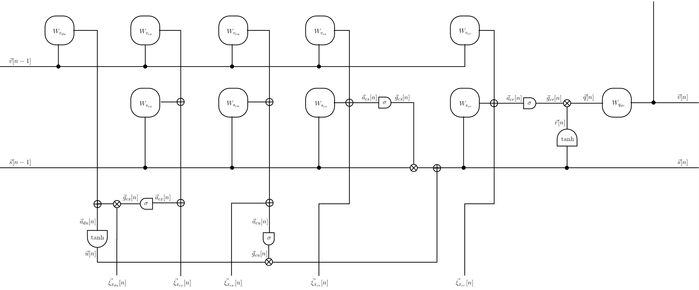
(a) Augmented LSTM network cell. The bias parameters, $\vec{b},$ have been omitted from the figure for brevity. They can be assumed to be included without
the loss of generality by appending an additional element, always set to $1$, to the input signal vector, $\vec{x}[n]$, and increasing the row dimensions of all
corresponding weight matrices by $1$. To minimize clutter in the diagram, the context windows are shown separately in Figure 10b below).

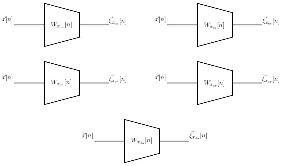
(b) The non-causal context windows, implemented as the convolutions (along the dimension of the sequence index, $n$) of the external input, $\vec{x}[n]$, with linear filters, whose coefficients are matrix-valued. The operations in this figure compute the quantities of the form ${\vec{\xi}_{x}[n]=W_{x}[n]\ast\vec{x}[n]}$, corresponding to their respective subscripts.

Figure 10: Augmented LSTM network cell system schematics.

VII-E Augmented LSTM System Derivatives: Backward Pass

The equations for training the Augmented LSTM cell, unrolled for $K$ steps, using BPTT, are obtained by adopting the same method as was used for the Vanilla LSTM cell in Section VI-I. We rely on the same border and intermediate total partial derivatives, appearing in Equations 140 – 144, with the addition of the total partial derivative of the objective function, $E$, with respect to the qualifier signal, $\vec{q}[n]$:

$$\vec{\beta}[n] \equiv\vec{\nabla}_{\vec{q}[n]}E=\frac{\partial E}{\partial\vec{q}[n]}$$ (219)

which is an intermediate total partial derivative that reflects the insertion of the projection layer into the cell’s data path. Applying the chain rule to the Augmented LSTM cell, defined by Equations 198 – 216, and judiciously utilizing all of these border and intermediate total partial derivatives, yields the backward pass equations for the Augmented LSTM cell:

$$\vec{\chi}[n] =\left(\frac{\partial\vec{y}[n]}{\partial\vec{v}[n]}\right)^{T}\left(\frac{\partial E}{\partial\vec{y}[n]}\right)+\vec{f_{\chi}}[n+1]$$ (220)

$$\vec{\beta}[n] =\left(\frac{\partial\vec{v}[n]}{\partial\vec{q}[n]}\right)^{T}\left(\frac{\partial E}{\partial\vec{v}[n]}\right)=W_{q_{dr}}^{T}\vec{\chi}[n]$$ (221)

$$\vec{\rho}[n] =\left(\frac{\partial\vec{q}[n]}{\partial\vec{r}[n]}\right)^{T}\left(\frac{\partial E}{\partial\vec{q}[n]}\right)=\vec{(\nabla}_{\vec{q}[n]}E)\odot\vec{g}_{cr}[n]=\vec{\beta}[n]\odot\vec{g}_{cr}[n]=W_{q_{dr}}^{T}\vec{\chi}[n]\odot\vec{g}_{cr}[n]$$ (222)

$$\vec{\gamma}_{cr}[n] =\frac{\partial E}{\partial\vec{q}[n]}\frac{\partial\vec{q}[n]}{\partial\vec{g}_{cr}[n]}=\vec{(\nabla}_{\vec{q}[n]}E)\odot\vec{r}[n]=\vec{\beta}[n]\odot\vec{r}[n]=W_{q_{dr}}^{T}\vec{\chi}[n]\odot\vec{r}[n]$$ (223)

$$\vec{\alpha}_{cr}[n] =\vec{\gamma}_{cr}[n]\odot\frac{\partial\vec{g}_{cr}[n]}{\partial\vec{a}_{cr}[n]}=\vec{\gamma}_{cr}[n]\odot\frac{dG_{c}(z)}{dz}\rfloor_{z=\vec{a}_{cr}[n]}=W_{q_{dr}}^{T}\vec{\chi}[n]\odot\vec{r}[n]\odot\frac{dG_{c}(z)}{dz}\rfloor_{z=\vec{a}_{cr}[n]}$$ (224)

$$\vec{\psi}[n] =\vec{\rho}[n]\odot\frac{\partial\vec{r}[n]}{\partial\vec{s}[n]}+\frac{\partial\vec{a}_{cr}[n]}{\partial\vec{s}[n]}\vec{\alpha}_{cr}[n]+\vec{f_{\psi}}[n+1]$$

$$=\vec{\rho}[n]\odot\frac{dG_{d}(\vec{z})}{d\vec{z}}\rfloor_{z=\vec{s}[n]}+W_{s_{cr}}\vec{\alpha}_{cr}[n]+\vec{f_{\psi}}[n+1]$$

$$=W_{q_{dr}}^{T}\vec{\chi}[n]\odot\vec{g}_{cr}[n]\odot\frac{dG_{d}(\vec{z})}{d\vec{z}}\rfloor_{z=\vec{s}[n]}+W_{s_{cr}}\vec{\alpha}_{cr}[n]+\vec{f_{\psi}}[n+1]$$ (225)

$$\vec{\alpha}_{cs}[n] =\vec{\psi}[n]\odot\frac{\partial\vec{s}[n]}{\partial\vec{g}_{cs}[n]}\odot\frac{\partial\vec{g}_{cs}[n]}{\partial\vec{a}_{cs}[n]}=\vec{\psi}[n]\odot\vec{s}[n-1]\odot\frac{dG_{c}(\vec{z})}{d\vec{z}}\rfloor_{z=\vec{a}_{cs}[n]}$$ (226)

$$\vec{\alpha}_{cu}[n] =\vec{\psi}[n]\odot\frac{\partial\vec{s}[n]}{\partial\vec{g}_{cu}[n]}\odot\frac{\partial\vec{g}_{cu}[n]}{\partial\vec{a}_{cu}[n]}=\vec{\psi}[n]\odot\vec{u}[n]\odot\frac{dG_{c}(\vec{z})}{d\vec{z}}\rfloor_{z=\vec{a}_{cu}[n]}$$ (227)

$$\vec{\alpha}_{du}[n] =\vec{\psi}[n]\odot\frac{\partial\vec{s}[n]}{\partial\vec{u}[n]}\odot\frac{dG_{d}(\vec{z})}{d\vec{z}}\rfloor_{z=\vec{a}_{du}[n]}=\vec{\psi}[n]\odot\vec{g}_{cu}[n]\odot\frac{dG_{d}(\vec{z})}{d\vec{z}}\rfloor_{z=\vec{a}_{du}[n]}$$ (228)

$$\vec{\gamma}_{cx}[n] =\vec{\alpha}_{du}[n]\frac{\partial\vec{u}[n]}{\partial\vec{g}_{cx}[n]}=\vec{\alpha}_{du}[n]\odot\vec{\xi}_{x_{du}}[n]$$ (229)

$$\vec{\alpha}_{cx}[n] =\vec{\gamma}_{cx}[n]\odot\frac{\partial\vec{g}_{cx}[n]}{\partial\vec{a}_{cx}[n]}=\vec{\gamma}_{cx}[n]\odot\frac{dG_{c}(z)}{dz}\rfloor_{z=\vec{a}_{cx}[n]}=\vec{\alpha}_{du}[n]\odot\vec{\xi}_{x_{du}}[n]\odot\frac{dG_{c}(z)}{dz}\rfloor_{z=\vec{a}_{cx}[n]}$$

$$=\vec{\psi}[n]\odot\vec{g}_{cu}[n]\odot\vec{\xi}_{x_{du}}[n]\odot\frac{dG_{d}(\vec{z})}{d\vec{z}}\rfloor_{z=\vec{a}_{du}[n]}\odot\frac{dG_{c}(z)}{dz}\rfloor_{z=\vec{a}_{cx}[n]}$$ (230)

where:

$$\vec{f_{\chi}}[n+1] =W_{v_{cu}}^{T}\vec{\alpha}_{cu}[n+1]+W_{v_{cs}}^{T}\vec{\alpha}_{cs}[n+1]+W_{v_{cr}}^{T}\vec{\alpha}_{cr}[n+1]+W_{v_{cx}}^{T}\vec{\alpha}_{cx}[n+1]+W_{v_{du}}^{T}\vec{\alpha}_{du}[n+1]$$ (231)

$$\vec{f_{\psi}}[n+1] =W_{s_{cu}}^{T}\vec{\alpha}_{cu}[n+1]+W_{s_{cs}}^{T}\vec{\alpha}_{cs}[n+1]+W_{s_{cx}}^{T}\vec{\alpha}_{cx}[n+1]+\vec{g}_{cs}[n+1]\odot\vec{\psi}[n+1]$$ (232)

Referring once again to the definition of the Augmented LSTM cell in Equations 198 – 216, we obtain:

$$\frac{\partial E}{\partial W_{x_{cu}}[l]}[n] =\vec{\alpha}_{cu}[n]\vec{x}^{T}[n+l]$$ (233)

$$\frac{\partial E}{\partial W_{s_{cu}}}[n] =\vec{\alpha}_{cu}[n]\vec{s}^{T}[n-1]$$ (234)

$$\frac{\partial E}{\partial W_{v_{cu}}}[n] =\vec{\alpha}_{cu}[n]\vec{v}^{T}[n-1]$$ (235)

$$\frac{\partial E}{\partial\vec{b}_{cu}}[n] =\vec{\alpha}_{cu}[n]$$ (236)

$$\frac{\partial E}{\partial W_{x_{cs}}[l]}[n] =\vec{\alpha}_{cs}[n]\vec{x}^{T}[n+l]$$ (237)

$$\frac{\partial E}{\partial W_{s_{cs}}}[n] =\vec{\alpha}_{cs}[n]\vec{s}^{T}[n-1]$$ (238)

$$\frac{\partial E}{\partial W_{v_{cs}}}[n] =\vec{\alpha}_{cs}[n]\vec{v}^{T}[n-1]$$ (239)

$$\frac{\partial E}{\partial\vec{b}_{cs}}[n] =\vec{\alpha}_{cs}[n]$$ (240)

$$\frac{\partial E}{\partial W_{x_{cr}}[l]}[n] =\vec{\alpha}_{cr}[n]\vec{x}^{T}[n+l]$$ (241)

$$\frac{\partial E}{\partial W_{s_{cr}}}[n] =\vec{\alpha}_{cr}[n]\vec{s}^{T}[n]$$ (242)

$$\frac{\partial E}{\partial W_{v_{cr}}}[n] =\vec{\alpha}_{cr}[n]\vec{v}^{T}[n-1]$$ (243)

$$\frac{\partial E}{\partial\vec{b}_{cr}}[n] =\vec{\alpha}_{cr}[n]$$ (244)

$$\frac{\partial E}{\partial W_{x_{cx}}[l]}[n] =\vec{\alpha}_{cx}[n]\vec{x}^{T}[n+l]$$ (245)

$$\frac{\partial E}{\partial W_{s_{cx}}}[n] =\vec{\alpha}_{cx}[n]\vec{s}^{T}[n-1]$$ (246)

$$\frac{\partial E}{\partial W_{v_{cx}}}[n] =\vec{\alpha}_{cx}[n]\vec{v}^{T}[n-1]$$ (247)

$$\frac{\partial E}{\partial\vec{b}_{cx}}[n] =\vec{\alpha}_{cx}[n]$$ (248)

$$\frac{\partial E}{\partial W_{x_{du}}[l]}[n] =\vec{\alpha}_{du}[n]\vec{x}^{T}[n+l]$$ (249)

$$\frac{\partial E}{\partial W_{v_{du}}}[n] =\vec{\alpha}_{du}[n]\vec{v}^{T}[n-1]$$ (250)

$$\frac{\partial E}{\partial\vec{b}_{du}}[n] =\vec{\alpha}_{du}[n]$$ (251)

$$\frac{\partial E}{\partial W_{q_{dr}}}[n] =\vec{\chi}[n]\vec{q}^{T}[n]$$ (252)

where $0\leq l\leq L-1$ and $0\leq n\leq K-1$. Arranged to parallel the structure of $\Theta$, defined in Equation 218, the total partial derivative of the objective function, $E$, with respect to the model parameters, $\Theta$, at the step with the index, $n$, is:

$$\begin{gathered}\frac{\partial E}{\partial\Theta}[n]=\end{gathered} \begin{Bmatrix}\frac{\partial E}{\partial W_{x_{cu}}[l]}[n],&\frac{\partial E}{\partial W_{s_{cu}}}[n],&\frac{\partial E}{\partial W_{v_{cu}}}[n],&\frac{\partial E}{\partial\vec{b}_{cu}}[n],\\ \frac{\partial E}{\partial W_{x_{cs}}[l]}[n],&\frac{\partial E}{\partial W_{s_{cs}}}[n],&\frac{\partial E}{\partial W_{v_{cs}}}[n],&\frac{\partial E}{\partial\vec{b}_{cs}}[n],\\ \frac{\partial E}{\partial W_{x_{cr}}[l]}[n],&\frac{\partial E}{\partial W_{s_{cr}}}[n],&\frac{\partial E}{\partial W_{v_{cr}}}[n],&\frac{\partial E}{\partial\vec{b}_{cr}}[n],\\ \frac{\partial E}{\partial W_{x_{cx}}[l]}[n]&\frac{\partial E}{\partial W_{s_{cx}}}[n]&\frac{\partial E}{\partial W_{v_{cx}}}[n]&\frac{\partial E}{\partial\vec{b}_{cx}}[n]\\ \frac{\partial E}{\partial W_{x_{du}}[l]}[n],&&\frac{\partial E}{\partial W_{v_{du}}}[n],&\frac{\partial E}{\partial\vec{b}_{du}}[n]\\ &&\frac{\partial E}{\partial W_{q_{dr}}}[n]\end{Bmatrix}.$$ (254)

Finally, $\frac{dE}{d\Theta}$, the total derivative of the objective function, $E$, with respect to the model parameters, $\Theta$, for the entire unrolled sequence is computed by Equation 174. Aggregated over a batch of segments, $\frac{dE}{d\Theta}$ is plugged in to the Gradient Descent training algorithm for learning the model parameters, $\Theta$.

VIII Conclusions and Future Work

In this paper, we presented the fundamentals of the RNN and the LSTM network using a principled approach. Starting with the differential equations encountered in many branches of science and engineering, we showed that the canonical formulation of the RNN can be obtained by sampling delay differential equations used to model processes in physics, life sciences, and neural networks. We proceeded to obtain the standard RNN formulation by appropriately choosing the parameters of the canonical RNN equations and applying stability considerations. We then formally explained RNN unrolling within the framework of approximating an IIR system by an FIR model and proved the sufficient conditions for its applicability to learning sequences. Next, we presented the training of the standard RNN using Back Propagation Through Time, segueing to the review of the vanishing and exploding gradients, the well-known numerical difficulties, associated with training the standard RNN by Gradient Descent. We subsequently addressed the shortcomings of the standard RNN by morphing the canonical RNN system into the more robust LSTM network through a series of extensions and embellishments. In addition to the logical construction of the Vanilla LSTM network from the canonical RNN, we included a self-contained overview of the Vanilla LSTM network, complete with the specifications of all principal entities as well as clear, descriptive, yet concise, presentations of the forward pass and, importantly, the backward pass, without skipping any steps. The main contribution up to this point has been our unique pedagogical approach for analyzing the RNN and Vanilla LSTM systems from the Signal Processing perspective, a formal derivation of the RNN unrolling procedure, and a thorough treatment using a descriptive and meaningful notation, aimed at demystifying the underlying concepts. Moreover, as an unexpected benefit of our analysis, we identified two novel extensions to the Vanilla LSTM network: the convolutional non-causal input context windows and the external input gate. We then augmented the equations for the LSTM cell with these extensions (along with the recurrent projection layer, previously introduced by another researcher team). Candidate recommendations for future work include implementing the Augmented LSTM system within a high-performance computing environment and benchmarking its efficacy in multiple practical scenarios. The use of the Augmented LSTM could potentially benefit the language representation subsystems used in question answering and in automating customer support. For these applications, it will be important to evaluate the performance impact, attributed to the non-causal input context windows, as compared to the different baselines, such the Vanilla LSTM network, the bi-directional LSTM network, the Transformer, and other state-of-the-art models. Also of particular relevance to this use case will be to measure the effectiveness of the external input gate in helping to eliminate the non-essential content from the input sequences. Finally, adopting the Augmented LSTM network to other practical domains and publishing the results is respectfully encouraged.

References

- [1] A.V. Oppenheim, R.W. Schafer. Discrete-time signal processing. Prentice-Hall, 1989.
- [2] Amar Gopal Bose. A Theory of Nonlinear Systems. PhD thesis, Massachusetts Institute of Technology, 1956.
- [3] Bo Chang, Minmin Chen, Eldad Haber, and Ed H. Chi. AntisymmetricRNN: A dynamical system view on recurrent neural networks. In International Conference on Learning Representations, Feb 2019.
- [4] Bo Chang, Lili Meng, Eldad Haber, Lars Ruthotto, David Begert, and Elliot Holtham. Reversible architectures for arbitrarily deep residual neural networks. In Sheila A. McIlraith and Kilian Q. Weinberger, editors, AAAI, pages 2811–2818. AAAI Press, 2018.
- [5] Edwin Chen. Exploring LSTMs. http://blog.echen.me/2017/05/30/exploring-lstms, 2017.
- [6] Tian Qi Chen, Yulia Rubanova, Jesse Bettencourt, and David Duvenaud. Neural Ordinary Differential Equations. In Samy Bengio, Hanna M. Wallach, Hugo Larochelle, Kristen Grauman, Nicoló Cesa-Bianchi, and Roman Garnett, editors, NeurIPS, pages 6572–6583, Dec 2018.
- [7] Leon O. Chua and Lin Yang. Cellular neural networks: Applications. IEEE Transactions on Circuits and Systems, 35:1273–1290, 1988.
- [8] Leon O. Chua and Lin Yang. Cellular neural networks: Theory. IEEE Transactions on Circuits and Systems, 35:1257–1272, 1988.
- [9] Marco Ciccone, Marco Gallieri, Jonathan Masci, Christian Osendorfer, and Faustino J. Gomez. Nais-net: Stable deep networks from non-autonomous differential equations. In Samy Bengio, Hanna M. Wallach, Hugo Larochelle, Kristen Grauman, Nicoló Cesa-Bianchi, and Roman Garnett, editors, NeurIPS, pages 3029–3039, Dec 2018.
- [10] B. de Vries and J. C. Principe. A theory for neural networks with time delays. In R. P. Lippmann, J. E. Moody, and D. S. Touretzky, editors, Advances in Neural Information Processing Systems 3, pages 162–168. Morgan Kaufmann, 1991.
- [11] J.L. Elman. Finding structure in time. Cognitive Science, 14:179–211, 1990.
- [12] Felix Gers. Long Short-Term Memory in Recurrent Neural Networks. PhD thesis, École Polytechnique Fédérale de Lausanne, 2001.
- [13] A. Graves and J. Schmidhuber. Framewise phoneme classification with bidirectional lstm and other neural network architectures. Neural Networks, 18(5-6):602–610, 2005.
- [14] A. Graves and J. Schmidhuber. Framewise phoneme classification with bidirectional LSTM networks. In Proc. Int. Joint Conf. on Neural Networks IJCNN 2005, 2005.
- [15] Alex Graves. Supervised sequence labelling with recurrent neural networks. PhD thesis, Technical University Munich, 2008.
- [16] Alex Graves. Generating sequences with recurrent neural networks. CoRR, abs/1308.0850, 2013.
- [17] Klaus Greff, Rupesh Kumar Srivastava, Jan Koutník, Bas R. Steunebrink, and Jürgen Schmidhuber. LSTM: A Search Space Odyssey. CoRR, abs/1503.04069, 2015.
- [18] S. Grossberg. Recurrent neural networks. Scholarpedia, 8(2):1888, 2013. revision #138057.
- [19] Stephen Grossberg. Nonlinear neural networks: Principles, mechanisms, and architectures. Neural Networks, 1:17–61, 1988.
- [20] Eldad Haber and Lars Ruthotto. Stable architectures for deep neural networks. Inverse Problems, 34(1):014004, 2017.
- [21] Sepp Hochreiter and Jürgen Schmidhuber. Long Short-Term memory. Neural computation, 9(8):1735–1780, 1997.
- [22] Sepp Hochreiter, Bengio Yoshua, Frasconi Paolo, and Jürgen Schmidhuber. Gradient flow in recurrent nets: the difficulty of learning long-term dependencies. In Kremer and Kolen, editors, A Field Guide to Dynamical Recurrent Neural Networks. IEEE Press, 2001.
- [23] J. J. Hopfield. Neurons with graded response have collective computational properties like those of two-state neurons. Proceedings of the National Academy of Sciences, 81:3088–3092, 1984.
- [24] Varuna Jayasiri. Vanilla LSTM with numpy. http://blog.varunajayasiri.com/numpy_lstm.html, 2017.
- [25] M. I. Jordan. Serial order: A parallel distributed processing approach. Technical Report ICS Report 8604, Institute for Cognitive Science, University of California, San Diego, 1986.
- [26] Anjuli Kannan, Karol Kurach, Sujith Ravi, Tobias Kaufmann, Andrew Tomkins, Balint Miklos, Greg Corrado, László Lukács, Marina Ganea, Peter Young, and Vivek Ramavajjala. Smart reply: Automated response suggestion for email. CoRR, abs/1606.04870, 2016.
- [27] Andrej Karpathy. The unreasonable effectiveness of recurrent neural networks. http://karpathy.github.io/2015/05/21/rnn-effectiveness, 2015.
- [28] Yuliya Kyrychko and Stephen Hogan. On the use of delay equations in engineering applications. 16:943–960, Jul 2010.
- [29] Omer Levy, Kenton Lee, Nicholas FitzGerald, and Luke Zettlemoyer. Long short-term memory as a dynamically computed element-wise weighted sum. CoRR, abs/1805.03716, May 2018.
- [30] Qianli Liao and Tomaso A. Poggio. Bridging the gaps between residual learning, recurrent neural networks and visual cortex. CoRR, abs/1604.03640, Apr 2016.
- [31] Henry W. Lin and Max Tegmark. Criticality in formal languages and statistical physics. Entropy, 19(7):299, Aug 2017.
- [32] Zachary Chase Lipton. A critical review of recurrent neural networks for sequence learning. CoRR, abs/1506.00019, 2015.
- [33] Yiping Lu, Aoxiao Zhong, Quanzheng Li, and Bin Dong. Beyond finite layer neural networks: Bridging deep architectures and numerical differential equations. In Jennifer G. Dy and Andreas Krause, editors, ICML, volume 80 of Proceedings of Machine Learning Research, pages 3282–3291. PMLR, Nov 2018.
- [34] Arun Mallya. Introduction to RNNs. http://slazebni.cs.illinois.edu/spring17/lec02_rnn.pdf, 2017.
- [35] Arun Mallya. LSTM Forward and Backward Pass. http://arunmallya.github.io/writeups/nn/lstm/index.html, 2017.
- [36] Arun Mallya. Some RNN Variants. http://slazebni.cs.illinois.edu/spring17/lec03_rnn.pdf, 2017.
- [37] J. H. McClellan, T. W. Parks, and L. R. Rabiner. A computer program for designing optimum fir linear phase digital filters. IEEE Transactions on Audio Electroacoustics, 21(6):506–526, 1973.
- [38] N. Metropolis, A. Rosenbluth, M. Rosenbluth, A. Teller, and E. Teller. Equation of state calculations by fast computing machines. J. Chem. Phys., 21:1087, 1953.
- [39] M.L. Minsky and S.A. Papert. Perceptrons. MIT Press, Cambridge MA, second edition, 1990.
- [40] Christopher Olah. Understanding LSTM Networks. http://colah.github.io/posts/2015-08-Understanding-LSTMs, 2015.
- [41] Oleksii Ostroverkhyi. Neural network processing of multidimensional signals. PhD thesis, Kharkiv National University of Radioelectronics, 2010.
- [42] Hamid Palangi, Li Deng, Yelong Shen, Jianfeng Gao, Xiaodong He, Jianshu Chen, Xinying Song, and Rabab K. Ward. Deep sentence embedding using the long short term memory network: Analysis and application to information retrieval. CoRR, abs/1502.06922, 2015.
- [43] Razvan Pascanu. On Recurrent and Deep Neural Networks. PhD thesis, Université de Montréal, 2014.
- [44] Razvan Pascanu, Tomas Mikolov, and Yoshua Bengio. On the difficulty of training recurrent neural networks. In International Conference on Machine Learning, pages 1310–1318, 2013.
- [45] Barak A. Pearlmutter. Learning state space trajectories in recurrent neural networks. Neural Computation, 1(2):263–269, 1989.
- [46] Barak A. Pearlmutter. Dynamic recurrent neural networks. Technical Report CMU-CS-90-196, Computer Science Department, Carnegie Mellon University, Pittsburgh, PA, 1990.
- [47] F. J. Pineda. Generalization of backpropagation to recurrent neural networks. Physical Review Letters, 59(19):2229–2232, 1987.
- [48] Fernando L. Pineda. Generalization of backpropagation to recurrent and higher order neural networks. In Dana Z. Anderson, editor, Neural Information Processing Systems, pages 602–611. New York: American Institute of Physics, 1987.
- [49] L. R. Rabiner. Techniques for designing finite-duration impulse-response digital filters. IEEE Transactions on Communications Technologies, 19(2):188–195, 1971.
- [50] Paul Renvoisé. Machine learning spotlight i: Investigating recurrent neural networks. https://recast.ai/blog/ml-spotlight-rnn/, 2017.
- [51] Yulia Rubanova, Ricky T. Q. Chen, and David Duvenaud. Latent odes for irregularly-sampled time series. Jul 2019. cite arxiv:1907.03907.
- [52] D. E. Rumelhart, G. E. Hinton, and R. J. Williams. Learning internal representations by error propagation. Technical Report DTIC Document, University of California San Diego, 1985.
- [53] D. E. Rumelhart and J. L. Mcclelland, editors. Parallel Distributed Processing, volume 1. MIT Press, 1986.
- [54] Lars Ruthotto and Eldad Haber. Deep neural networks motivated by partial differential equations. CoRR, abs/1804.04272, 2018.
- [55] Hasim Sak, Andrew W. Senior, and Françoise Beaufays. Long short-term memory recurrent neural network architectures for large scale acoustic modeling. In Haizhou Li, Helen M. Meng, Bin Ma, Engsiong Chng, and Lei Xie, editors, Interspeech, pages 338–342. ISCA, 2014.
- [56] Hojjat Salehinejad, Julianne Baarbe, Sharan Sankar, Joseph Barfett, Errol Colak, and Shahrokh Valaee. Recent advances in recurrent neural networks. CoRR, abs/1801.01078, 2018.
- [57] Terence D. Sanger. Optimal unsupervised learning in a single-layer linear feedforward neural network. Neural Networks, 2:459–473, 1989.
- [58] Mike Schuster and Kuldip K. Paliwal. Bidirectional recurrent neural networks. IEEE Transactions on Signal Processing, 45:2673–2681, November 1997.
- [59] Alex Sherstinsky. M-Lattice: A System For Signal Synthesis And Processing Based On Reaction-Diffusion. PhD thesis, Massachusetts Institute of Technology, 1994.
- [60] Alex Sherstinsky. Deriving the Recurrent Neural Network Definition and RNN Unrolling Using Signal Processing. In Critiquing and Correcting Trends in Machine Learning Workshop at Neural Information Processing Systems 31 (NeurIPS 2018), Dec 2018. Organizers: Benjamin Bloem-Reddy, Brooks Paige, Matt J. Kusner, Rich Caruana, Tom Rainforth, and Yee Whye Teh.
- [61] Alex Sherstinsky. Fundamentals of Recurrent Neural Network (RNN) and Long Short-Term Memory (LSTM) Network, 2018. cite arxiv:1808.03314.
- [62] Alex Sherstinsky and Rosalind W. Picard. M-lattice: from morphogenesis to image processing. IEEE Transactions on Image Processing, 5(7):1137–1149, 1996.
- [63] Alex Sherstinsky and Rosalind W. Picard. On the efficiency of the orthogonal least squares training method for radial basis function networks. IEEE Transactions on Neural Networks, 7(1):195–200, 1996.
- [64] Alex Sherstinsky and Rosalind W. Picard. On stability and equilibria of the M-Lattice. IEEE Transactions on Circuits and Systems – I: Fundamental Theory and Applications, 45(4):408–415, 1998.
- [65] S. H. Strogatz. Nonlinear Dynamics and Chaos. Westview Press, Cambridge, MA, 1994.
- [66] Martin Sundermeyer, Ralf Schlüter, and Hermann Ney. LSTM Neural Networks for Language Modeling. In Interspeech, pages 194–197, 2012.
- [67] Ilya Sutskever. Training Recurrent Neural Networks. PhD thesis, University of Toronto, 2012.
- [68] Ilya Sutskever, James Martens, and Geoffrey E. Hinton. Generating text with recurrent neural networks. In Lise Getoor and Tobias Scheffer, editors, ICML, pages 1017–1024. Omnipress, 2011.
- [69] Ilya Sutskever, Oriol Vinyals, and Quoc V Le. Sequence to sequence learning with neural networks. In Advances in neural information processing systems, pages 3104–3112, 2014.
- [70] Lloyd N. Trefethen. Finite Difference and Spectral Methods for Ordinary and Partial Differential Equations. unpublished text, Cambridge, MA, 1996.
- [71] Oriol Vinyals. Beyond Deep Learning: Scalable Methods and Models for Learning. PhD thesis, EECS Department, University of California, Berkeley, Dec 2013.
- [72] Yu Wang. A new concept using LSTM neural networks for dynamic system identification. In ACC, pages 5324–5329. IEEE, 2017.
- [73] P. Werbos. Backpropagation through time: what does it do and how to do it. In Proceedings of IEEE, volume 78, pages 1550–1560, 1990.
- [74] P. J. Werbos. Generalization of backpropagation with application to a recurrent gas market model. Neural Networks, 1, 1988.
- [75] Ronald J. Williams and David Zipser. A learning algorithm for continually running fully recurrent neural networks. Neural Computation, 1:270–280, 1989.
- [76] Y. Yamamoto, B. D. O. Anderson, M. Nagahara, and Y. Koyanagi. Optimizing fir approximation for discrete-time iir filters. IEEE Signal Processing Letters, 10(9):273–276, Sep 2003.
- [77] Wojciech Zaremba, Ilya Sutskever, and Oriol Vinyals. Recurrent neural network regularization, 2014. cite arxiv:1409.2329.
- [78] Jie Zhou, Ying Cao, Xuguang Wang, Peng Li, and Wei Xu. Deep recurrent models with fast-forward connections for neural machine translation. CoRR, abs/1606.04199, 2016.