Nonparametric Gaussian Mixture Models
for the Multi-Armed Bandit
Abstract
We here adopt Bayesian nonparametric mixture models to extend multi-armed bandits in general, and Thompson sampling in particular, to scenarios where there is reward model uncertainty. In the stochastic multi-armed bandit, where an agent must learn a policy that maximizes long term payoff, the reward for the selected action is generated from an unknown distribution. Reward uncertainty, i.e., the lack of knowledge about the reward-generating distribution, induces the exploration-exploitation trade-off: a bandit agent needs to simultaneously learn the properties of the reward distribution and sequentially decide which action to take next. Thompson sampling is a bandit algorithm that requires knowledge of the true reward model, for sampling from its parameter posterior and calculation of per-arm expected rewards. In this work, we extend Thompson sampling to scenarios where there is reward model uncertainty by adopting Bayesian nonparametric Gaussian mixture models for flexible reward density estimation. By characterizing each arm’s reward distribution with independent Bayesian nonparametric mixture models, the per-arm nonparametric distribution adjusts its complexity as new bandit rewards are observed, which is used for guiding the agent’s subsequent arm selections. The proposed Bayesian nonparametric mixture model Thompson sampling sequentially learns the reward model that best approximates the true, yet unknown, per-arm reward distribution, achieving successful regret performance. We derive, based on a novel posterior convergence based analysis, an asymptotic regret bound for the proposed method. In addition, we empirically evaluate its performance in diverse and previously elusive bandit environments, e.g., with rewards not in the exponential family, subject to outliers, and with different per-arm reward distributions, and show that it outperforms, both in averaged cumulative regret and in regret volatility, state-of-the-art alternatives. The proposed Bayesian nonparametric Thompson sampling is valuable in the presence of reward model uncertainty, as it avoids stringent case-by-case model design choices, yet provides important regret savings.
1 Introduction
Sequential decision making aims to optimize interactions with the world (exploit), while simultaneously learning how the world operates (explore). The multi-armed bandit (MAB) (Lattimore and Szepesvári, 2020) is a natural abstraction for a wide variety of real-world challenges that require learning while simultaneously maximizing rewards (Lai and Robbins, 1985). The name ‘bandit’ finds its origin in the playing strategy one must devise when facing a row of slot machines. The contextual MAB, where at each interaction with the world side information (known as ‘context’) is available, is a natural extension of the bandit problem. The study of the exploration-exploitation trade-off can be traced back to the beginning of the past century, with important contributions by Thompson (1935), Robbins (1952) and Lai and Robbins (1985). Recently, a renaissance of the study of MAB algorithms has flourished (Slivkins, 2019; Lattimore and Szepesvári, 2020), attracting interest for its application in science, medicine, engineering, business and operations research (Li et al., 2010; Villar et al., 2015; Hill et al., 2017; Aziz et al., 2021). In practice, bandit applications are personalized via the contextual MAB paradigm, and often deal continuous observations: e.g., to measure dwell time in online advertising and content recommendation, or to quantify drug responses in clinical trials.
Among the many bandit algorithms available, Thompson (1933) sampling provides an elegant approach to tackle the exploration-exploitation dilemma. It updates a posterior over expected rewards for each arm, and chooses actions based on the probability that they are optimal. It has been empirically and theoretically proven to perform competitively for MAB models within the exponential family (Agrawal and Goyal, 2013b, a; Korda et al., 2013). Its applicability to the more general reinforcement learning setting of Markov decision processes (Burnetas and Katehakis, 1997) has tracked momentum as well (Gopalan and Mannor, 2015; Ouyang et al., 2017). A Thompson sampling policy requires access to posterior samples of the true reward model. Unfortunately, maintaining such posterior is intractable for distributions not in the exponential family (Russo et al., 2018). Therefore, developing practical MAB methods to balance exploration and exploitation in domains that do not pertain to such a reward family remains largely unsolved.
In an effort to extend Thompson sampling to complex bandit scenarios, where the true reward model distribution is often unknown, researchers have considered neural-network based reward functions with Bayesian inference (Riquelme et al., 2018), bootstrapping (Osband and Roy, 2015) and ensembling (Lu and Roy, 2017) based techniques —a detailed overview of state-of-the art MAB methods is provided in Section 2.1. On the contrary, the novelty of this work is on exploiting Bayesian nonparametric (BNP) mixture models for Thompson sampling to perform MAB optimization under reward model uncertainty.
We here adopt the Bayesian generative view of Thompson sampling, and argue that modeling bandit reward distributions via BNP mixtures —which can estimate continuous reward distributions and adjust model complexity to the observed distribution of rewards— can provide successful bandit performance. Even if, for bandit regret minimization, proper modeling of the full reward distributions may not be in general necessary, we defend that a statistical modeling-based approach, which leverages the advances on nonparametric density estimation within statistics, can be performant in the multi-armed bandit setting. Note that we are not interested in nonparametric priors over arms (whether continuous or discrete), but in MABs with a discrete set of actions, for which there is uncertainty on the per-arm reward function. To that end, we incorporate BNP mixture models into Thompson Sampling, and develop an algorithm that —without incurring model misspecification— adapts to a wide variety of complex bandits and attains reduced regret.
We model each of the bandit arm reward distributions with per-arm BNP mixture models. By means of BNP mixture models, where one uses nonparametric prior distributions such as Dirichlet or Pitman-Yor processes (Pitman and Yor, 1997) over the mixing proportions, we can accurately approximate continuous reward distributions. For learning such a nonparametric distribution within the MAB setting, we leverage well-established advances for inference in BNP models (Neal, 2000). These enable analytically tractable posterior updates, which allow for sequential adjustment of the complexity of the BNP reward model to the observed bandit data.
It is both the combination of BNP mixture models with Thompson sampling (i.e., merging a state-of-the art bandit algorithm with nonparametric statistical advances), as well as the resulting flexibility and generality (i.e., avoiding model misspecification while providing performance guarantees) that is novel and significant in this work. To the best of our knowledge, no other work uses Bayesian nonparametric mixtures to model independent, per-arm reward distributions in MABs. Our specific contributions are:
-
1.
To propose a unique, yet flexible Thompson sampling bandit method that resolves reward model uncertainty: the agent learns the Bayesian nonparametric mixture model that best approximates the true, but unknown, per-arm reward distribution, adjusting its complexity as it sequentially observes data.
-
2.
An asymptotic regret bound for the proposed Thompson sampling algorithm of order , when assuming a Dirichlet process Gaussian mixture model per-arm, where denotes the number of bandit arms, the number of agent iterations with the environment, and the constant depends on the tail behavior of the true reward distribution and the prior base measure of the Dirichlet process. Our posterior convergence-based proof technique is conceptually simple yet general enough to be applied for the analysis of Thompson sampling with other reward distributions.
-
3.
To demonstrate empirically that the proposed nonparametric Thompson sampling:
-
(a)
attains reduced regret in complex MABs under reward model uncertainty —for multimodal, exponential and heavy tailed reward distributions, with different unknown per-arm distributions— when compared to state-of-the art bandit algorithms; and
-
(b)
performs equivalently to the Oracle Thompson sampling, i.e., the agent that knows the true underlying model class.
-
(a)
Our contributions are valuable in practice, i.e., for bandit scenarios in the presence of model uncertainty: the same bandit algorithm is readily applicable, and attains reduced regret, in unknown and complex (e.g., not in the exponential family) multi-armed bandits. The proposed Thompson sampling method, as it nonparametrically adjusts its reward posterior distribution to the observed bandit data, avoids case-by-case reward model design choices, bypassing model misspecification and hyperparameter tuning.
The paper is structured as follows. Section 2 contains preliminaries on multi-armed bandits and Thompson sampling (2.1); as well as on Bayesian nonparametric models and the Dirichlet process (2.2). In Section 3, we describe the proposed BNP bandit reward model (3.1), with details on the reward predictive posterior (3.1.1) and the mixture parameter posteriors (3.1.2). We present the nonparametric Gaussian mixture model based Thompson sampling, referred to as Nonparametric TS, in Section 3.2, for which we provide a regret bound in Section 3.2.1 for Dirichlet process priors. Section 4 highlights the empirical performance success of the proposed method in a set of diverse and complex bandit scenarios. We conclude with Section 5, where we summarize our work and discuss future research directions. Proofs, inference and implementation details, additional simulation studies, as well as a real-life evaluation are deferred to the Appendix.
2 Background
2.1 Multi-armed bandits and Thompson sampling
Background.
A multi-armed bandit (MAB) is a real time sequential decision process in which, at each interaction with the world, an agent selects an action (i.e., arm) , where is the set of arms of the bandit, according to a policy targeted to maximize cumulative rewards over time. The (stochastic) rewards observed by the agent are independent and identically distributed (i.i.d.) from the true, yet unknown, outcome distribution , where 111The argument of a distribution denotes the random variable, which is capitalized, its realizations are denoted in lower-case. is the joint probability distribution of rewards, itself randomly drawn from a family of distributions . Reward distributions are often parameterized by , i.e., , where the true reward distribution corresponds to a unique : . Without loss of generality, we relate to the parametric notation hereafter, and in a Bayesian view of MABs, specify a prior with hyperparameter over the parameter distribution when necessary (we will omit the hyperparameters of the prior when it is clear from context). We denote with the conditional reward distribution of arm , from which outcomes are drawn: .
Contextual bandits.
In the contextual MAB, an agent must decide which arm to play at each time , based on the available context , where the observed reward for the played arm is drawn from the unknown reward distribution of arm conditioned on the context,
| (1) |
Given the true model , the optimal action is to select
| (2) |
where
| (3) |
is the conditional expectation of rewards with respect to the true reward distribution of each arm , given context at time , and true parameter .
Exploration-exploitation tradeoff.
The challenge in (contextual) MABs is the lack of knowledge about the reward-generating distribution, i.e., uncertainty about (or about in the parametric case) induces uncertainty about the true optimal action . One needs to simultaneously learn the properties of the reward distribution —its expected value, at a minimum— and sequentially decide which action to take next. Optimizing interactions with the world (exploit), while simultaneously learning how the world operates (explore), requires a balance between both. To that end, a bandit agent must devise and execute a bandit policy that balances this exploration-exploitation tradeoff.
Bandit policy and regret.
We use to denote a bandit policy, which is in general stochastic ( is a random variable) on its choices of arms: . MAB policies choose the next arm to play towards maximizing (expected) rewards, based upon the history observed. Previous history contains the set of given contexts, played arms, and observed rewards up to time , denoted as , with , , and , where denotes the reward observed after playing arm at time . The goal is to maximize a policy’s cumulative reward, or equivalently, to minimize the cumulative regret (the loss incurred due to not knowing the best arm at each time ), i.e.,
| (4) |
where denotes the optimal arm choice and the arm selected by policy at time .
In the stochastic MAB setting, we study the expected cumulative frequentist regret at time horizon ,
| (5) |
where the expectation is taken over the randomness of the outcomes —for a given true parametric model — and the arm selection policies : denotes the optimal policy, denotes an stochastic bandit policy. For clarity of notation, we drop the dependency on context from and , as these are fixed and observed for all .
A related notion of regret, where the uncertainty in the true bandit model is averaged over an assumed model prior , is known as the expected cumulative Bayesian regret at time horizon ,
| (6) |
Bayesian regret has been considered by many for the analysis of MAB algorithms (Bubeck and Liu, 2013; Russo and Roy, 2014, 2016), but as pointed out by (Agrawal and Goyal, 2013a), a regret bound on the frequentist sense implies the same bound on Bayesian regret, but not vice-versa.
Thompson sampling.
Thompson sampling (TS) (Thompson, 1933; Russo et al., 2018) is a stochastic policy that chooses what arm to play next in proportion to its probability of being optimal, given the history up to time , i.e.,
| (7) |
where we specifically denote with a subscript p the parametric model class assumed by a Thompson sampling policy .
In a Bayesian view of MABs, the uncertainty over the reward model —the unknown parameter — is accounted for by modeling it as a random variable with an appropriate prior with hyperparameters .
The goal in Thompson sampling is to compute the probability of an arm being optimal by marginalizing over the posterior probability distribution of the unknown model parameter after observing history ,
| (8) |
The above integral marginalizes the uncertainty over the parameter posterior (of the assumed model class ) given history . However, the challenge with the integral in Equation (8) is that it cannot be solved exactly, even when the parameter posterior is analytically tractable over time.
Instead, Thompson sampling draws a random parameter sample from the updated posterior , and picks the arm that maximizes the expected reward given the drawn parameter sample,
| (9) |
Thompson sampling for complex models.
Extending Thompson sampling to complex reward distributions, specifically those not in the exponential family, is an active area of research. In general, two themes emerge: one where the true reward distribution is the object of analysis, another where only the per-arm reward means are of interest.
A promising approach of the former is to embrace Bayesian neural networks with approximate inference, where flexible estimation of the unknown reward distribution is pursued. To that end, variational methods, stochastic mini-batches, and Monte Carlo techniques have been studied (Blundell et al., 2015; Kingma et al., 2015; Lipton et al., 2018; Osband et al., 2016; Li et al., 2016), where uncertainty estimation of reward posteriors has been shown to be critical for successful bandit performance. In parallel, others have focused on a generative view of Thompson sampling, and have targeted new reward model classes, such as maintaining and incrementally updating an ensemble of plausible models that approximates the intractable posterior distribution of interest (Lu and Roy, 2017); or approximating the unknown bandit reward function with finite Gaussian mixture models (Urteaga and Wiggins, 2018).
On the contrary, several authors have argued for empirically estimating per-arm bandit reward means, with a follow-the-perturbed-leader exploration approach for bandit optimization. This (non-generative) view of Thompson sampling relies on the notion that posterior sampling can be formulated as a perturbation scheme that is sufficiently optimistic, as originally noted by Agrawal and Goyal (2013a, b). Since then, bootstrapping techniques that use a combination of observed and artificially generated data have been proposed for MAB and reinforcement learning problems (Osband and Roy, 2015; Eckles and Kaptein, 2019).
We here explore the Bayesian generative modeling view of bandits and Thompson sampling, as it facilitates not only interpretable modeling, but sequential and batch processing as well.
Thompson sampling and Bayesian nonparametrics.
Bayesian nonparametric models have been considered in MAB problems to accommodate both continuous and countable many MAB actions. For instance, (Srinivas et al., 2010; Grünewälder et al., 2010; Krause and Ong, 2011) model a continuum of MAB actions via Gaussian processes (GPs), which are powerful nonparametric prior distributions over continuous functions (Rasmussen and Williams, 2005). Hierarchical Pitman-Yor processes have been used to model an unknown yet countable number of MAB actions (Battiston et al., 2018), or to optimize budget allocation for single-cell sequential experiment designs to maximize the number of new cell types discovered (Camerlenghi et al., 2020).
On the contrary, we are not interested in maximizing reward diversity or having a continuum (or a countably infinite number) of arms, but in MABs with a discrete set of actions, for which there is uncertainty on the per-arm reward function. In the following, we investigate Bayesian nonparametric mixture models as tractable yet performant distributions for estimating unknown reward densities.
2.2 Bayesian nonparametric mixture models
Background.
A Bayesian nonparametric (BNP) model is a Bayesian model on an infinite-dimensional parameter space, typically chosen as the set of possible solutions for a learning problem (Hjort et al., 2010; Müller et al., 2015). In regression problems, the parameter space can be the set of continuous functions —e.g., specified via a prior correlation structure in Gaussian process regression (Rasmussen and Williams, 2005); and in density estimation problems, the hypothesis space can consist of all the densities with continuous support —e.g., a Dirichlet Process Gaussian mixture model (Escobar and West, 1995). A Bayesian nonparametric model uses only a finite subset of the available parameter dimensions to explain a finite set of observations, with the set of dimensions adjusted according to the observed sample, such that the effective complexity of the model (as measured by the number of dimensions used) adapts to the data. The BNP modeling approach is to fit a single model to the data, yet to allow the BNP model to grow its complexity as more data is observed. Classic adaptive problems, such as nonparametric density estimation and model selection, can be formulated as BNP inference problems. Here, we leverage Bayesian nonparametric mixture modeling as a powerful density estimation framework that adjust model complexity in response to the observed data (Ghosal and der Vaart, 2017).
Nonparametric mixture models for density estimation.
Modeling a distribution as a mixture of simpler distributions is a common approach to density estimation, where determining the number of mixtures is often addressed via model selection. On the contrary, BNP models describe a countably infinite number of components via a nonparametric prior distribution for the model components. BNP mixture models provide a powerful approach to density estimation, because they do not only avoid specifying the number of mixtures beforehand, but allow for an unbounded number of mixtures to appear as more data is observed. A BNP model, as in any Bayesian model, starts with a random (nonparametric) prior distribution which, after observing some data from the likelihood function, induces a (nonparametric) posterior distribution (Ghosal, 2010). Strong posterior convergence results of BNP models for density estimation have been already established: i.e., for a wide class of continuous distributions, and under mild regularity conditions, the BNP posterior converges to the true data-generating density (Ghosal et al., 1999; Ghosal and van der Vaart, 2001; Lijoi et al., 2004; Tokdar, 2006; Ghosal and van der Vaart, 2007; Bhattacharya and Dunson, 2010; Pati et al., 2013).
Dirichlet process mixture models.
In a Bayesian mixture model, we model the distribution from which data is drawn as a mixture of (parametric) distributions , where the mixing distribution over is denoted as , and we specify a prior over . In a Dirichlet process mixture model, we define the prior for the mixing distribution to be a Dirichlet process (Ferguson, 1973). The Dirichlet process (DP) is a distribution over distributions, parameterized by a concentration parameter and a base measure over a space . A random draw from a DP is itself a distribution over , which we denote as .
The generative process of the DP mixture model follows
| (10) | ||||
| (11) | ||||
| (12) |
The DP was introduced by Ferguson (1973), who proved its existence and many of the properties that are fundamental for their use as priors for BNP mixture models; e.g., random distributions drawn from the DP are discrete with probability one. As such, can be viewed as a countably infinite random mixture (Ferguson, 1973; Neal, 2000), where random probability mass is placed on a countably infinite collection of points, called atoms:
| (13) |
is the Dirac delta function located at atom , and is the probability assigned to the th atom. The sequence of random atoms is i.i.d. from the base measure .
Sethuraman (1994) showed that we can construct random distributions as in Equation (13) with distribution , if and for , for a sequence of independent, beta-distributed random variables . This representation is known as the “stick-breaking construction” of the DP (Gershman and Blei, 2012).
In addition, Ferguson (1973) showed that, when marginalizing over random distributions drawn from a DP,
| (14) |
the joint distribution over a sequence of parameters exhibits a clustering property (they share repeated values with positive probability): i.e., for an i.i.d. random sample of size drawn from a DP process, there will be ties within parameter samples (not all samples will be different). Instead, there will be distinct samples , each with multiplicities .
The distribution of the corresponding partition is a Chinese restaurant process (Teh and Jordan, 2010; Gershman and Blei, 2012), which allows to obtain a representation of the DP in terms of successive conditional distributions (Blackwell and MacQueen, 1973; Neal, 2000):
| (15) |
where refers to the multiplicity of each distinct sample , with .
Equation (15) determines the probabilities, conditioned on the sequence , of observing () a previously instantiated parameter , (), which grows with the number of observations in each partition ; and () a non-zero probability () of observing a ‘new’ parameter drawn from the base measure .
After observations drawn from a DP, there are already ‘seen’ atoms, and as we observe more data, the number of distinct atoms grows. Consequently, the more samples we draw from a DP process, the higher the probability of observing it again in the future. A DP process has a ‘rich get richer’ behavior that scales the number of distinct clusters logarithmically: (Antoniak, 1974).
Pitman-Yor processes and Pitman-Yor mixture models.
There exist several generalizations of the DP: e.g., the Pitman-Yor process —which allows for modeling power-law distributed data— and Pólya Trees (Mauldin et al., 1992) —that can generate both discrete and piecewise continuous densities. A Pitman-Yor (PY) process (Pitman and Yor, 1997), denoted as with discount parameter , concentration parameter , and a base measure , is a stochastic process whose sample path is a probability distribution, . The discount parameter gives the PY process more flexibility over tail behavior: the DP has exponential tails, whereas the PY can have power-law tails (Ishwaran and James, 2001), which may be suitable in many practical applications. In this work, we focus on Dirichlet process mixture models, and explicitly indicate possible extensions via Pitman-Yor processes to power-law distributed data when appropriate.
3 Bayesian nonparametric Thompson sampling
We combine Bayesian nonparametric mixture models with Thompson sampling for MABs under reward model uncertainty. At every interaction, bandit reward is i.i.d. drawn from a true, context dependent distribution of the played arm — a distribution unknown to the bandit agent.
We model and estimate these unknown per-arm reward distributions with Bayesian nonparametric mixture models. For a collection of observed context, actions and rewards at time , , we fit a BNP model to the observed data, and use the BNP posterior predictive distribution to guide the agent’s next arm selection.
3.1 Per-arm rewards as Dirichlet process Gaussian mixture models
We pose per-arm, independent DP Gaussian mixture models for context-conditional rewards, with the following nonparametric generative process:
| (16) | ||||
| (17) | ||||
| (18) |
where for the i.i.d. parameters drawn from the DP process, we adopt a normal inverse-gamma base measure 222 This base measure is used due to its conjugacy to the context-conditional Gaussian distribution of rewards, which will facilitate posterior computation and inference.
| (19) |
with hyperparameters .
The graphical model of the Bayesian nonparametric bandit is rendered in Figure 1, where we showcase the independence between each arm’s reward distribution: we accommodate different reward distributions for each MAB arm .
Modeling rationale.
We study the classic MAB with per-arm i.i.d. rewards, and characterize each arm’s unknown reward distribution with distinct per-arm BNP models . The mixture parameters for each arm are different, drawn from per-arm specific Dirichlet Processes, . Consequently, we enjoy full flexibility to estimate each arm’s reward distribution independently, addressing MABs with diverse reward model classes per-arm. This setting, where we accommodate distinct per-arm reward distributions, is a powerful extension of the MAB problem, which has not attracted interest so far, yet can circumvent model misspecification.
An alternative BNP model would be to consider a hierarchical nonparametric model (Teh et al., 2006; Teh and Jordan, 2010), which we outline in Section A of the Appendix. This alternative introduces dependencies between bandit arms, as all arms obey the same algebraic family of distributions: because the base measure is common to the observations from all arms, there is information sharing across arms. On the contrary, we study independent per-arm BNP mixture model reward distributions as in Equation (16)–(18), and leave the theoretical and empirical study of hierarchical alternatives as future work.
3.1.1 Per-arm rewards’ predictive posterior
We now present per-arm DP mixture models’ posterior predictive distribution , of interest for the development of a Thompson sampling policy with BNP reward distributions as in Equations (16)–(18).
Let us denote with the sequence of time-instants where arm has been played up to time instant , for a total of , with . We write for the sequence of rewards observed when bandit arm is played, i.e., . Given a set of observed context, actions and rewards, , after marginalizing out , we obtain the following per-arm conditional predictive reward distribution:
| (20) | ||||
| (21) |
With a slight abuse of notation, we denote with the collection of all DP mixture parameters in the predictive distribution,
| (22) |
where indicates the number of rewards observed at time from playing arm that are drawn from mixture : . To keep track of which distinct mixture component each observation is drawn from, auxiliary latent variables are introduced —see Section 3.2.2 for a procedure on inferring and updating these.
The clustering property and the data-dependent model complexity of the DP (as discussed in Section 2.2) is evident from the predictive distribution in Equation (21): the next reward from arm will be drawn from either one of the already instantiated mixture “atoms” with distinct parameters , or from a new mixture component with parameters drawn from the base measure, .
The number of distinct mixture components per-arm is determined by the DP process, as a function of the observed per-arm rewards . Therefore, the effective complexity of the reward model adapts to the observed bandit data over time: each per-arm DP mixture model will accommodate as many components — in Equation (21)— as necessary to best describe the observed per-arm bandit rewards .
3.1.2 Per-arm rewards’ parameter posterior
The BNP mixture parameters in Equation (22) are not observed in practice, i.e., they are latent variables of the BNP model. We capture the uncertainty on these unobserved parameters via their posterior distributions. These are computed based on per-arm base measure priors in Equation (19), by incorporating information from the per-arm observed rewards .
Due to the conjugate form of the base measure —a normal inverse-gamma in Equation (19)— and the per-arm reward emission distributions —context-conditional Gaussian densities in Equation (18)— the posterior of per-arm distinct parameters , , follow a normal inverse-gamma distribution
| (23) |
with hyperparameters
| (24) |
where is a sparse diagonal matrix with elements for and indicates the number of rewards observed when playing arm up to time that are assigned to mixture component . The above expression can be computed sequentially as data are observed for the played arm.
3.2 Nonparametric Gaussian mixture model Thompson sampling
We leverage the BNP, context-conditional Gaussian mixture model of Equations (16)–(18) and derive a posterior sampling MAB policy, i.e., a BNP Thompson sampling.
At each interaction with the world, the proposed nonparametric Thompson sampling —detailed in Algorithm 1— decides which arm to play next based on the predictive distribution in Equation (21), computed using a random parameter sample drawn from the BNP parameter posteriors in Equations (23)–(24).
The proposed nonparametric Thompson sampling policy draws posterior nonparametric parameter samples given history , and picks the arm that maximizes its expected reward
| (25) |
Due to the nonparametric nature of the DP mixture predictive posterior distribution, parameters for both distinct and new potential mixture components are drawn,
| (26) |
with posterior hyperparameters for already instantiated distinct parameters as in Equation (24), along with prior hyperparameters over a potential new parameter in Equation (19).
Given these samples , and according to the DP mixture model predictive distribution of Equation (21), the agent can readily compute the expected per-arm reward,
| (27) |
Pitman-Yor mixture model based Thompson sampling.
The proposed DP mixture model based Thompson sampling is readily generalizable to Pitman–Yor mixture models.
3.2.1 Analysis of nonparametric Gaussian mixture model Thompson sampling
We here prove a regret bound for the proposed nonparametric mixture model based Thompson sampling. We first provide a key lemma and outline our proposed posterior convergence based analysis of Thompson sampling. We then specialize the analysis to bound the regret of Thompson sampling with Dirichlet process priors and Gaussian emission distributions.
Posterior convergence based analysis of Thompson sampling.
A Thompson sampling policy operates according to the probability of each arm being optimal. Inspection of such probability in Equation (8) results on an equivalence with the expectation of the optimal arm indicator function, with respect to the joint posterior distribution of the expected rewards given history and context, , i.e.,
The indicator function for each arm requires the posterior over all arms. That is, the posterior is the joint posterior distribution over the expected rewards of all arms, : it is a dimensional multivariate distribution over all arms of the bandit.
Before presenting our first lemma, we recall that the total variation distance between distributions and on a sigma-algebra of subsets of the sample space is defined as
| (31) |
which is properly defined for both discrete and continuous distributions (see details in Section B of the Appendix). We now present our lemma, with the proof provided in Section B of the Appendix.
Lemma 3.1.
The difference in action probabilities between two Thompson sampling policies under reward distributions and , given the same history and context up to time , is bounded by the total-variation distance between the posterior distributions of their expected rewards at time , and , respectively,
This lemma enables a posterior convergence based cumulative regret analysis of Thompson sampling policies as follows:
| (32) | ||||
| (33) | ||||
| (34) |
The approach consists of expressing the regret of Thompson sampling policies as the difference between their action probabilities —Equation (33)— which allows for using Lemma 3.1 —Equation (34)— to express regret in terms of the total variation distance between posterior densities. Therefore, a bound on the total variation distance bounds the cumulative regret.
Regret bound for Dirichlet process Gaussian mixture Thompson sampling.
We make use of Lemma 3.1 to asymptotically bound the cumulative regret of the proposed Thompson sampling with Dirichlet process priors and Gaussian emission distributions as in Equations (16)–(18), for bandits with true reward densities that meet certain regularity conditions. The analysis relies on leveraging asymptotic BNP posterior convergence rates, i.e., the rate at which the distance between two densities becomes small as the number of observations grows. As we asymptotically bound the total variation distance between the true and the BNP reward posterior, we can then bound the regret of the proposed nonparametric Thompson sampling.
Theorem 3.2.
The expected cumulative regret at time of a Dirichlet process Gaussian mixture model based Thompson sampling algorithm is, for , asymptotically bounded by
We use big-O notation for the asymptotic regret bound, as it bounds from above the growth of the cumulative regret over time for large enough bandit interactions, i.e.,
| (35) |
This bound holds both in a frequentist and Bayesian view of expected regret.
The proof of Theorem 3.2, provided in Section B of the Appendix, amounts to bounding the regret introduced by two factors: the first, related to the use of an Oracle Thompson sampling (i.e., a policy that does not know the true parameters of the reward distribution, but has knowledge of the true reward model class); and the second, a term that accounts for the convergence of the posterior of a BNP reward model to that of the true data generating distribution.
The logarithmic term in the bound appears due to the convergence rate of the BNP posteriors to the truth, where the exponent depends on the tail behavior of the base measure and the priors of the Dirichlet process —see Section B of the Appendix for details on posterior density convergence and its impact on the exponent .
Regret bound for Pitman-Yor mixture model based Thompson sampling.
The bound presented in Theorem 3.2 is specific to per-arm Dirichlet process mixture models, as these are nonparametric priors on densities with strong results on how the BNP posterior converges to the true density at the minimax-optimal rate, up to logarithmic factors (Ghosal, 2010).
Because, to the best of our knowledge, there is a lack of general results on the PY mixture model posterior convergence —as stated by Jang et al. (2010), “not all of the (PY) sampling priors produce consistent posteriors”— extension of the regret bound to the PY mixture model assumption is not pursued here.
3.2.2 Inference of per-arm rewards’ DP mixture model posterior
For the proposed nonparametric Thompson sampling to operate successfully, we must compute and draw from per-arm DP mixture model posteriors, for which inference of the unknown latent variables , given observations , is needed. The Bayesian inference literature provides plenty of alternatives to do so, based on Markov Chain Monte Carlo (Neal, 2000), sequential Monte Carlo (Fearnhead, 2004) and variational alternatives (Blei and Jordan, 2004). Any of these techniques that infer the assignment variables and results in density convergence is adequate for execution in line 14 of Algorithm 1.
We here describe and implement a marginalized Gibbs sampler —equivalent to algorithm 3 presented by Neal (2000)— that iterates between sampling assignments and updates to the emission distribution’s hyperparameters . The pseudo-code is presented in Algorithm 2 and is succinctly described hereafter —the full procedure is detailed in Section C of the Appendix.
Marginalized Gibbs sampler.
As a new reward is observed for the arm played at time , the BNP mixture model is updated based on the Gibbs sampling procedure of Algorithm 2 . We iterate through to determine each per-arm rewards’ assignments to distinct, already instantiated, mixture components ; or a new mixture component —Line 7 in Algorithm 2. The Gibbs sampler autonomously adjusts the posterior’s complexity (i.e., number of mixture components ) according to the observed per-arm rewards. Given these inferred assignments , we recompute sufficient statistics —Line 8 in Algorithm 2— and update parameter posteriors —Line 9 in Algorithm 2. The Gibbs sampler is run until a stopping criteria is met —Line 5 in Algorithm 2: either the marginalized log-likelihood of the observed rewards and sampled assignments given updated hyperparameters is stable within an relative log-likelihood margin between consecutive iterations, or a maximum number of iterations is reached.
Warm-started Gibbs sampler.
Due to the sequential acquisition of rewards in the bandit setting —a single arm is played at each bandit interaction— only the posterior for the played arm needs to be updated at time . As such, even though the Gibbs sampler might be initialized with prior hyperparameters at every interaction, we propose to instead use the DP hyperparameters and inferred assignments for all but this latest observed reward as input to Algorithm 2: i.e., assignments and hyperparameters inferred based on the already observed rewards, . Consequently, the Gibbs sampler is warm-started at each bandit interaction with good hyperparameters and latent assignments (that describe all but this newly observed reward ), so that good convergence can be achieved in few iterations per observed reward.
Computational complexity.
Since Equation (24) can be sequentially computed for each per-arm observation, the computational cost of the Gibbs sampler in Algorithm 2 grows with the number of rewards observed for the played arm , with . Therefore, the overall computational cost is upper-bounded by per-interaction with the world, i.e., per newly observed reward .
In practice, and because of the warm-start, one can limit the number of Gibbs sampler iterations per-bandit interaction to upper-bound the algorithm’s complexity to per MAB interaction with the environment 333 Note that, as reported by Fearnhead (2004), the computational cost of running a Gibbs sampler for iterations is similar to running a sequential Monte Carlo method with particles., yet achieve satisfactory performance —empirical evidence of this claim is provided in Section E of the Appendix. We emphasize that the Gibbs sampler shall run until log-likelihood convergence, and only suggest limiting the number of Gibbs iterations to as a practical recommendation with upper-bounded computational complexity and good empirical regret performance.
4 Evaluation
We evaluate the proposed nonparametric Gaussian mixture model Thompson sampling, denoted Nonparametric TS, in diverse and complex bandit scenarios summarized in Table 1, for which practical methods that balance exploration and exploitation remain elusive.
We validate the performance of Nonparametric TS for Gaussian bandits in Section 4.2, and tackle Gaussian mixture modeled rewards in Section 4.3, rewards subject to outliers in Section 4.4, and exponentially distributed rewards in Section 4.5. We study different reward model classes per-arm and the impact of model misspecification. An application to a very challenging, real-world dataset from clinical oncology is included in Section H.
| Scenario | Section | Oracle TS |
|---|---|---|
| Gaussian bandits | Appendix Section D | Agrawal and Goyal (2012) |
| Linear Gaussian bandits | Section 4.2 | Agrawal and Goyal (2013b) |
| Gaussian Mixture model bandits | Section 4.3 | Urteaga and Wiggins (2018) |
| Heavy-tailed bandits | Section 4.4 | Urteaga and Wiggins (2018) |
| Exponentially distributed bandits | Section 4.5 | N/A |
| Precision oncology bandit | Appendix Section H | N/A |
We evaluate Nonparametric TS in comparison not only to state-of-the-art alternatives (described next in Section 4.1) but to Oracle Thompson sampling policies that know the true underlying model class. By comparing the performance of Nonparametric TS to Oracle TS policies, we scrutinize the flexibility of the proposed Bayesian nonparametric approach for per-arm reward model estimation. The goal is to showcase whether the proposed policy incurs any regret penalty due to its BNP reward modeling assumption.
Assuming knowledge of a bandit’s reward distribution is unrealistic, yet possible in simulated environments. With simulated bandits, we have access to ground truth, and therefore, the possibility to compare the proposed algorithm to both an Optimal policy (that knows which arm is the best in hindsight) and an Oracle policy (that knows the true reward model).
4.1 Thompson sampling-based baselines
We implement Nonparametric TS as in Algorithm 1, assuming a Dirichlet process prior —the BNP mixture model for which we have provided theoretical guarantees in Theorem 3.2— with concentration parameter (sensitivity analysis results for different are provided in Section F of the Appendix). Nonparametric TS implements the Gibbs sampler described in Algorithm 2, with and , for all the experiments. An empirical evaluation of Nonparametric TS with different values is provided in Section E of the Appendix.
We compare Nonparametric TS to several alternative Thompson sampling policies. The algorithms listed below are state-of-the art techniques that provide different computations of (or approximations to) reward posteriors that can be combined with Thompson sampling to address complex contextual bandits.
-
1.
LinearGaussian TS: A powerful (not neural network based) Thompson sampling baseline, which assumes a contextual linear Gaussian reward function,
In its simplest setting, when the reward variance is known, the resulting Thompson sampling implementation follows that by Agrawal and Goyal (2013b). In our experiments, in a similar fashion as done by Riquelme et al. (2018), we model the joint distribution of and , , which allows the method to adaptively adjust to the observed reward noise. We leverage the normal inverse-gamma conjugate prior, i.e.,
(36) of the Gaussian contextual model to derive the exact Bayesian posterior. We use an uninformative prior for the variance () and a standard uncorrelated Gaussian for the mean prior ().
-
2.
MultitaskGP: This is an alternative and popular Bayesian nonparametric technique that models context to reward mappings via Gaussian processes (Srinivas et al., 2010; Grünewälder et al., 2010; Krause and Ong, 2011). This implementation regresses the expected reward of different context-actions pairs by fitting a multi-task Gaussian process given observed bandit data.
-
3.
NeuralLinear: This algorithm, introduced by Riquelme et al. (2018), operates by learning a neural network that maps contexts to rewards for each action, and simultaneously, updates a Bayesian linear regression in the network’s last layer that maps a learned representation linearly to the rewards . The corresponding Thompson sampling draws the learned linear regression parameters for each arm, but keeps the representation output by the learned network. In our experiments, the representation network and the Bayesian linear posterior are retrained and updated at every MAB interaction.
-
4.
NeuralBootstrapped: This algorithm is based on (Osband et al., 2016), which trains simultaneously and in parallel neural networks based on different bootstrapped bandit histories . These are generated by adding each newly observed evidence to each history , , independently and with probability . In order to choose an action for a given context, one of the networks is selected with uniform probability (), and the best action according to the selected network is played.
-
5.
NeuralRMS: This is a bandit benchmark that trains a neural network to map contexts to rewards. At each time , it acts -greedily according to the current model, which due to the Stochastic Gradient Descent (SGD) algorithm used for training (the RMSProp optimizer in this implementation), captures randomness in its output.
-
6.
NeuralDropoutRMS: Dropout is a neural network training technique where the output of each neuron is independently zeroed out with a given probability in each forward pass. Once the network is trained, dropout can also be used to obtain a distribution of predictions for a specific input. By choosing the best action with respect to the random dropout prediction, an implicit form of Thompson sampling is executed.
-
7.
NeuralParamNoise: An approach to approximate a distribution over neural networks is to randomly perturb the point estimates attained by SGD on the available data Plappert et al. (2018). In this case, the model uses a heuristic to control the amount of i.i.d. noise it adds to the neural network parameters, which is used for making a decision, but not for training: SGD re-starts from the last, noiseless parameter value.
-
8.
BNNVariationalGaussian: This algorithm is based on ideas presented in Blundell et al. (2015) that combine stochastic variational inference and Bayes by backpropagation. It implements a Bayesian neural network by modeling each individual weight posterior as a univariate Gaussian distribution. Thompson sampling then draws a network at each time step by sampling each weight independently. The variational approach consists in maximizing a proxy for the maximum likelihood estimates of the network weights given observed data, to fit the unknown parameters of the variational posterior.
-
9.
BNNAlphaDiv: This technique leverages expectation/propagation and Black/box alpha/divergence minimization as in Hernandez-Lobato et al. (2016) to approximate the unknown reward distribution. The algorithm iteratively approximates the posterior of interest by updating a single approximation factor at a time, which usually corresponds to the likelihood of one data point. The implementation adopted here optimizes the global objective directly via stochastic gradient descent.
-
10.
Oracle TS: We implement state-of-the-art Oracle Thompson Sampling policies for each evaluated bandit scenario, where the Oracles know the true per-arm reward distributions of the bandit they are targeted to. We detail in Table 1 which Thompson sampling is appropriate (with references to the original work) for each bandit.
-
11.
Optimal: When possible (i.e., for simulated bandits for which there is ground truth), we implement an optimal multi-armed bandit policy that selects the best arm for the given context, based on the known true expected reward of each arm.
For completeness and reproducibility, we present the set of hyperparameters used for our experiments in Section I of the Appendix, and note that a full description of these baseline algorithms and their implementation can be found in the deep bandit showdown work.
4.2 Contextual linear Gaussian bandits
We first investigate the classic contextual linear Gaussian MAB, where rewards are drawn from linearly parameterized arms, where the mean reward for context and arm is given by , for some unknown latent parameter . We compare Nonparametric TS to the alternatives described in Section 4.1 in Section 4.2.1, and to the Oracle TS in Section 4.2.2. Results for the non-contextual Gaussian MAB are provided in Section D of the Appendix, where we showcase how the proposed method attains satisfactory performance, when compared to the Oracle policy.
In the following, we evaluate different parameterizations of contextual linear Gaussian bandits, and scrutinize the impact of the dimensionality and sparsity (i.e., how many components of are non-zero) of the arms in bandit regret performance.
4.2.1 Comparison to baselines
We hereby evaluate regret for contextual linear Gaussian bandits with arms. The context is 10 dimensional, distributed as independent standard Gaussians, and we draw a 10 dimensional uniformly at random —with only 3 non-zero components for each arm parameter in the sparse setting. In all cases, Gaussian noise (with a minimum standard deviation of 0.01) is added to the rewards of each arm.
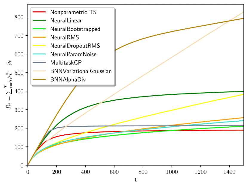
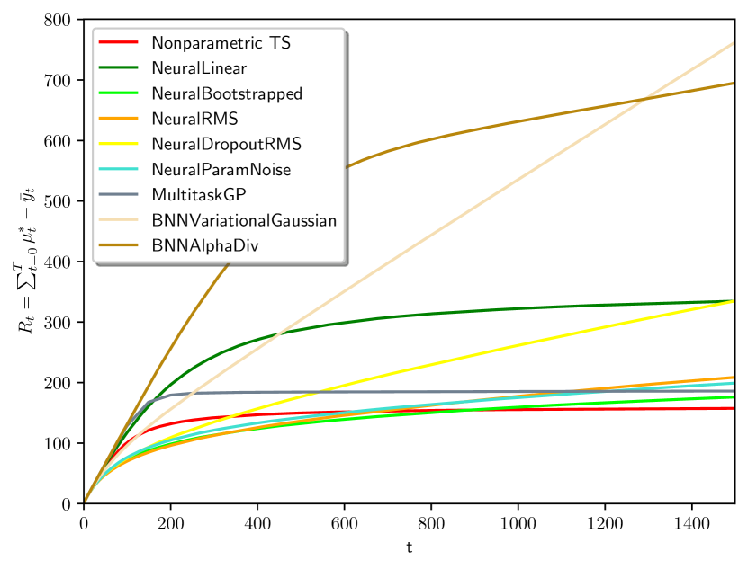
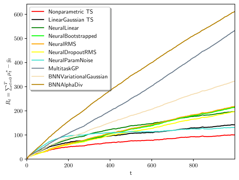
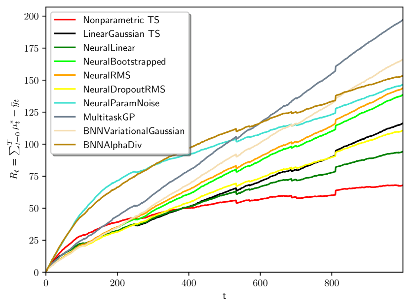
Figure 2 showcases the expected cumulative regret of all algorithms in non-sparse and sparse linear contextual bandits, respectively. Detailed mean and standard deviation results, along with attained relative cumulative regret improvements, are provided in Table 2.
| Algorithm | Linear Gaussian | Sparse Linear Gaussian |
|---|---|---|
| Nonparametric TS | 189.889 12.980 (0.000%) | 157.406 12.430 (0.000%) |
| NeuralLinear | 398.485 18.219 (109.852%) | 334.569 16.400 (112.551%) |
| NeuralBootstrapped | 210.914 47.416 (11.073%) | 176.136 46.643 (11.899%) |
| NeuralRMS | 256.897 69.191 (35.288%) | 208.738 64.960 (32.611%) |
| NeuralDropoutRMS | 382.870 87.055 (101.629%) | 334.870 92.306 (112.742%) |
| NeuralParamNoise | 241.039 59.296 (26.937%) | 199.122 62.129 (26.502%) |
| MultitaskGP | 213.648 22.006 (12.512%) | 186.023 21.026 (18.180%) |
| BNNVariationalGaussian | 827.369 193.087 (335.712%) | 762.321 203.467 (384.301%) |
| BNNAlphaDiv | 793.118 43.457 (317.675%) | 695.097 39.556 (341.594%) |
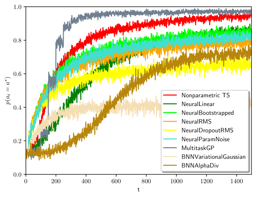
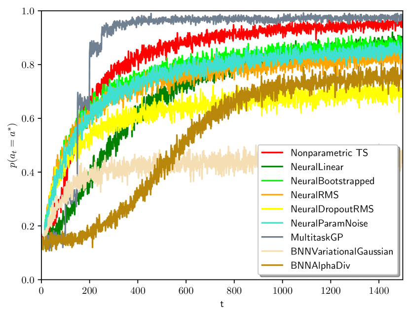
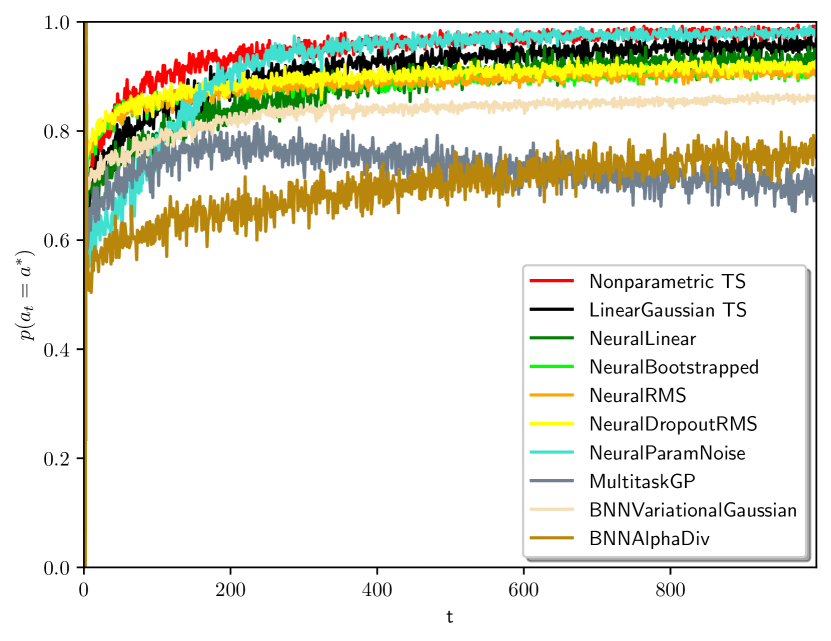
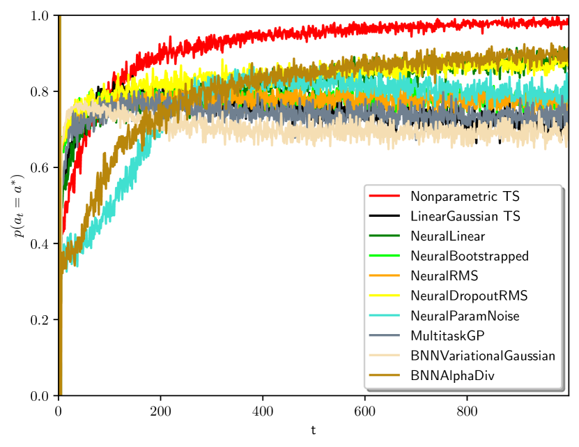
First, we observe that the proposed Nonparametric TS method finds a satisfactory exploration-exploitation balance i.e., it achieves logarithmic cumulative regret as observed in Figures 2(a) and 2(b), even as it estimates the true form of the underlying unknown reward function. MultitaskGP and NeuralLinear alternatives showcase a plateaued cumulative regret curve as well: i.e., as shown in Figure 3, MultitaskGP and Nonparametric TS are the only policies that quickly learn to play the optimal arm with high-probability —NeuralLinear eventually catches up. Note the one-to-one mapping between finding the best bandit arm, and a plateaued cumulative regret curve: once the algorithm identifies the best arm, incurred instant regret goes to zero and the algorithm’s cumulative regret flattens.
Second, we observe reduced cumulative regret of the proposed Nonparametric TS when compared to all state-of-the-art Thompson sampling alternatives: MultitaskGP incurs 18% more cumulative regret, while the neural network based linear Thompson sampling method (NeuralLinear) doubles the cumulative regret of Nonparametric TS at . Bootstrapped and RMS based alternatives fail to achieve a good exploration-exploitation trade-off: as shown in Figure 3, they fail to consistently play the optimal arm, which results in a cumulative regret that does not plateau in either Figure 2(a) or 2(b). This results in cumulative regrets that are at least 10% and 30% higher at time in all contextual MABs. Recall the poor performance of all the Bayesian Neural Network (BNN) based baselines, which incur in more than 300% cumulative regret increase with respect to the proposed Nonparametric TS.
We finally notice a very volatile performance of these noise-injecting policies across realizations of the same problem —the standard deviation of the empirical cumulative regrets is considerably higher: 46.64 for NeuralBootstrapped, 64.96 for NeuralRMS, 92.31 for NeuralDropoutRMS and 62.13 for NeuralParamNoise in the sparse linear Gaussian MAB.
4.2.2 Comparison to Oracle TS
, .

, .
, .
.
.
.
,
.
,
.
,
.
,
.
,
.
,
.
We compare the performance of Nonparametric TS to the LinearGaussian TS in Agrawal and Goyal (2013b), which correctly assumes the true underlying contextual linear Gaussian model , and computes posterior updates in closed form.
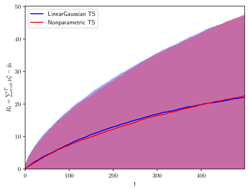
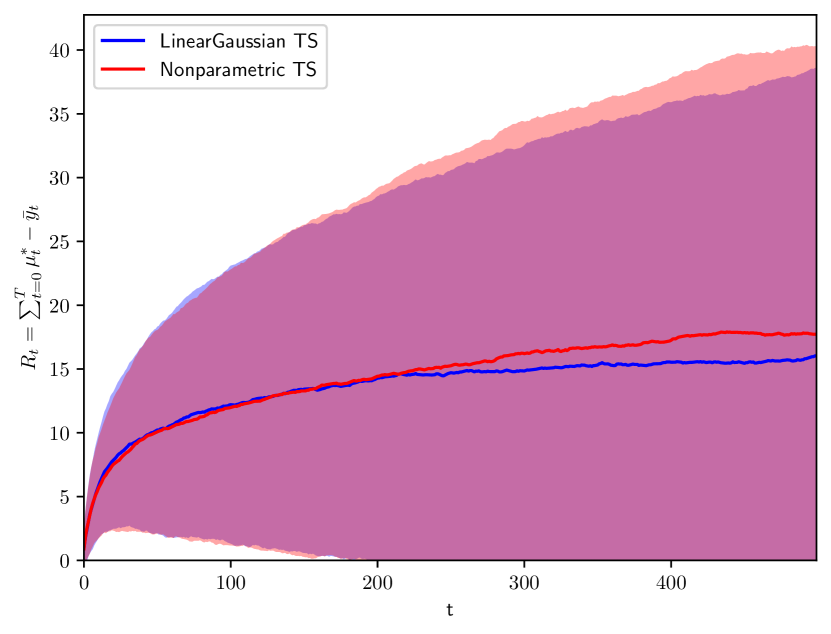
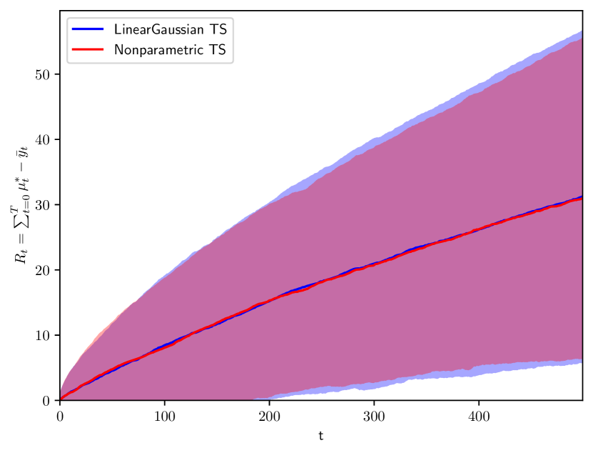
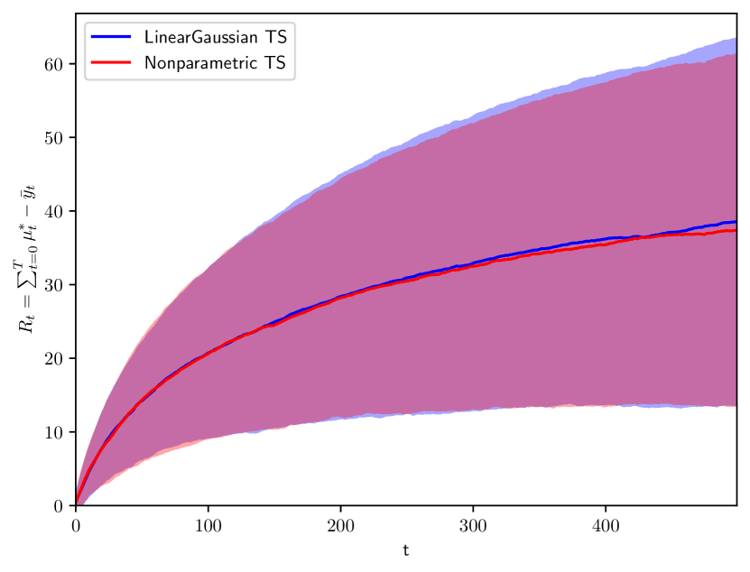
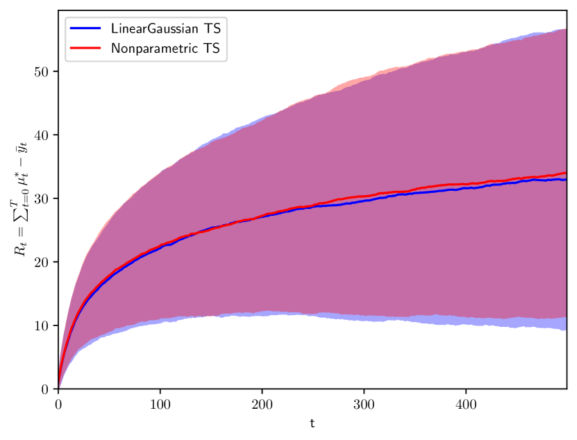
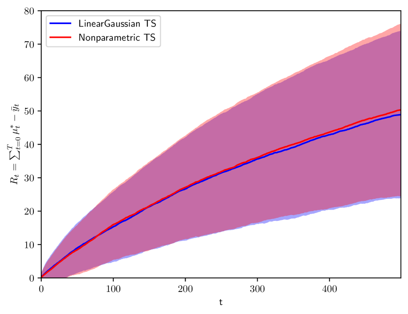
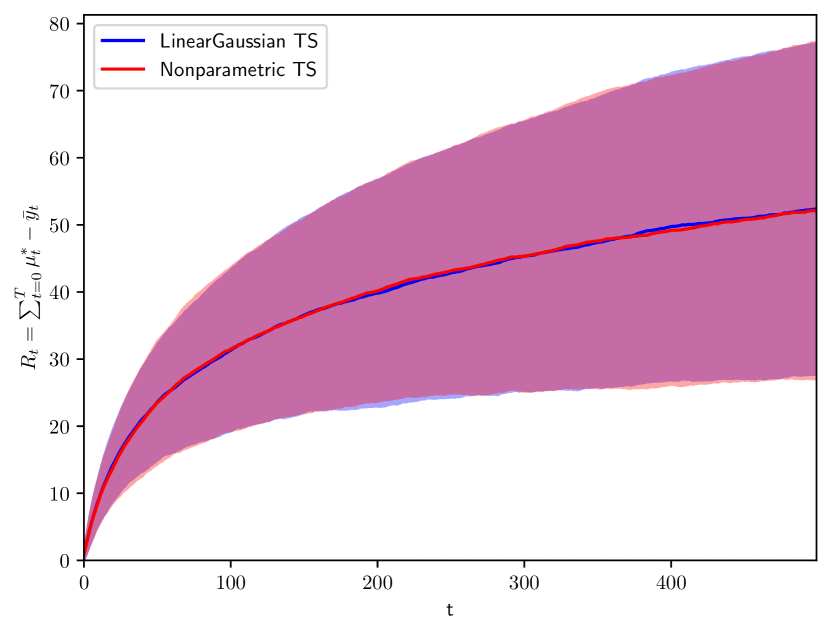
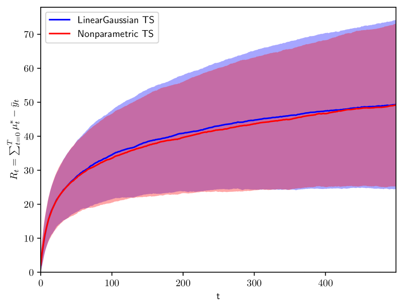
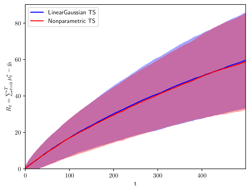
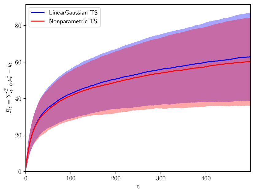
In Figure 4 in the next page, we show cumulative regret for several parameterizations of multi-armed, , contextual linear Gaussian bandits, with two-dimensional contexts randomly drawn from a uniform distribution: , , .
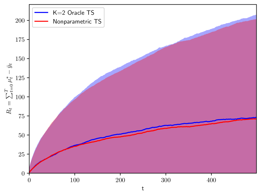
Across all parameterizations, Nonparametric TS attains cumulative regret comparable (both in expectation and in volatility) to that of the Oracle TS, i.e., LinearGaussian TS: Nonparametric TS matches the performance of the analytical linear Gaussian posterior Thompson sampling, even as it nonparametrically estimates the unknown, true reward distribution. The proposed nonparametric method is as good as the analytical, Oracle alternative when there is no model mismatch: the per-arm nonparametric predictive posterior quickly converges to the true unknown distribution, incurring in minimal additional regret when compared to the analytical Oracle TS.
4.3 Contextual Gaussian mixture model bandits
We now study more challenging, and previously elusive, contextual MABs where the underlying reward distributions do not fit into the exponential family assumption. We simulate the following contextual Gaussian mixture model bandits, where the context is randomly drawn from a two dimensional uniform distribution, i.e., , , :
Scenario A:
Scenario B:
The reward distributions of the contextual bandits in these simulated scenarios are Gaussian mixtures, which differ in the amount of mixture overlap and the similarity between arms.
Scenario A is a mixture of two Gaussian distributions, where there is a significant overlap between arm rewards. Note the unbalanced nature of the mixture in arm 2: rewards from a mixture component with low expected value are drawn with probability , and higher rewards are expected with probability .
Scenario B describes a MAB with different per-arm reward distributions: a linear Gaussian distribution for arm 1, a bi-modal Gaussian mixture for arm 2, and an unbalanced Gaussian mixture with three components for arm 3. Rewards for each arm of this bandit are drawn from different distributions, a MAB setting not previously addressed in the literature.
We scrutinize Nonparametric TS by comparing it to TS baselines in Section 4.3.1, and to Oracle TS algorithms for Gaussian mixture models in Section 4.3.2.
4.3.1 Comparison to baselines
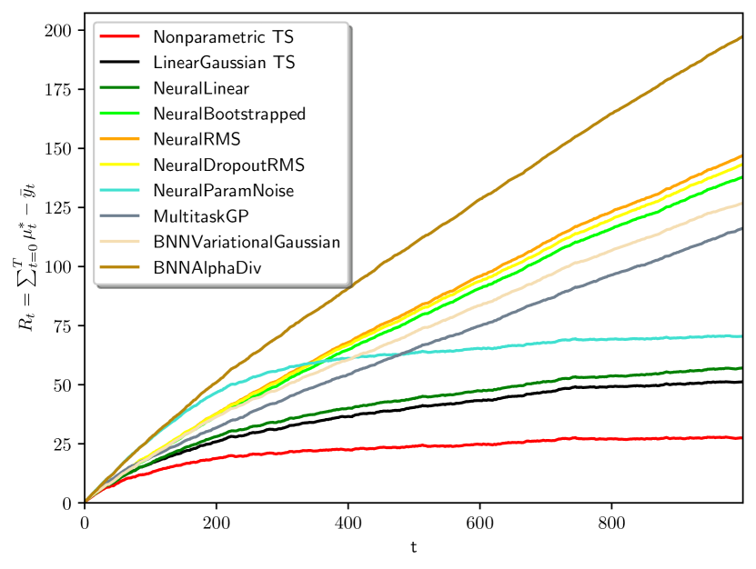
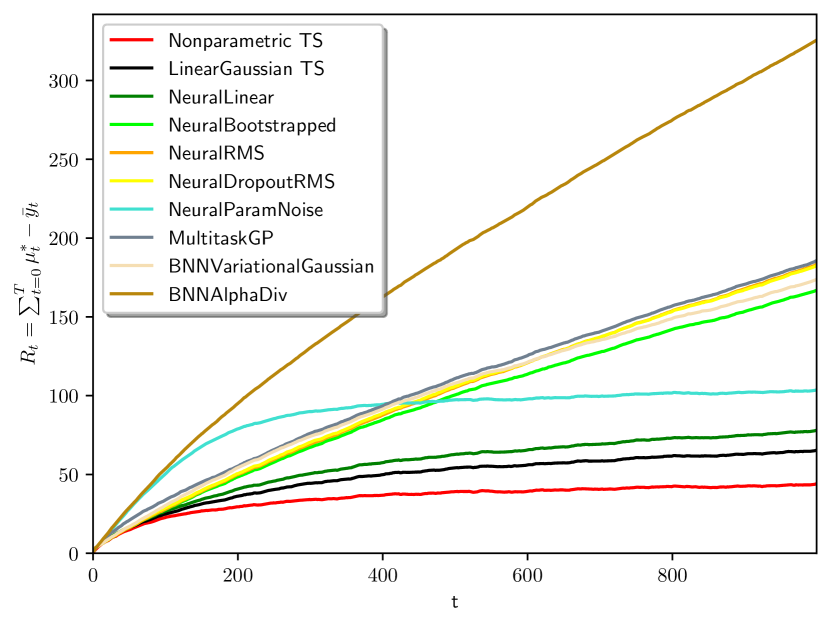
We show in Figure 5 how our proposed Nonparametric TS seamlessly adjusts to the true reward model, attaining reduced cumulative regret, when compared to all implemented alternatives. Detailed cumulative regret results (mean, standard deviation and relative regret improvements) are provided in Table 3.
| Algorithm | Scenario A | Scenario B |
|---|---|---|
| Nonparametric TS | 27.467 70.723 (0.000%) | 44.114 70.391 (0.000%) |
| LinearGaussian TS | 51.236 99.308 (86.539%) | 65.422 89.903 (48.304%) |
| NeuralLinear | 57.029 91.606 (107.630%) | 78.081 94.970 (77.000%) |
| NeuralBootstrapped | 137.878 220.172 (401.982%) | 166.907 267.797 (278.357%) |
| NeuralRMS | 147.014 227.547 (435.242%) | 183.307 282.358 (315.536%) |
| NeuralDropoutRMS | 143.284 224.607 (421.666%) | 182.552 282.107 (313.823%) |
| NeuralParamNoise | 70.493 71.740 (156.649%) | 103.703 72.562 (135.082%) |
| MultitaskGP | 116.178 99.036 (322.977%) | 185.676 152.088 (320.906%) |
| BNNVariationalGaussian | 126.860 229.256 (361.868%) | 173.787 293.195 (293.954%) |
| BNNAlphaDiv | 197.361 66.569 (618.545%) | 325.655 68.638 (638.221%) |
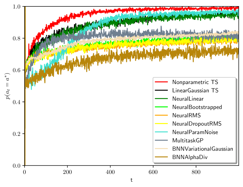
Notice that few bandit algorithms are able to find the right exploitation-exploration balance (i.e., plateaued cumulative regret curves in Figure 5): only Nonparametric TS, LinearGaussian, NeuralLinear and NeuralParamNoise achieve so. This is corroborated by the empirical frequencies of playing the optimal arm shown in Figure 6, where we observe how the rest of the policies are not able to find the optimal arm, even after many bandit interactions.
Nonparametric TS is the best policy (i.e., learns to play the optimal arm the fastest), incurring in considerable regret reduction: NeuralLinear attains 107.63% and 77.00% more cumulative regret in Scenarios A and B. NeuralLinear takes longer to reach the exploration-exploitation tradeoff —in par with the simpler LinearGaussian alternative.
We do not observe any competitive advantage of neural-network based alternatives in Scenarios A and B, i.e., for rewards drawn from distributions not in the exponential family. Bootstrapped and RMS based neural Thompson sampling techniques struggle to find a good exploration-exploitation balance, incurring in additional and very volatile regret performance, as shown in Figure 5 and detailed in Table 3. These noise-injection based methods seem to be unable to disentangle model training from better exploration in these challenging bandit settings. Variational inference, expectation-propagation and Gaussian process based algorithms also perform poorly (see Table 3). The inability to accurately adapt (either due to model misspecification or to optimization challenges) to the rewards drawn from a mixture model may explain this phenomena. Beyond the expected cumulative regret limitations, the volatility of the evaluated neural network based alternatives is also noteworthy —see standard deviation results in Table 3, showcasing a highly variable performance.
On the contrary, Nonparametric TS outperforms (both in averaged cumulative regret, and in regret volatility) all alternatives across bandits with mixture model rewards, even with different per-arm reward distributions, without any scenario-specific fine-tuning.
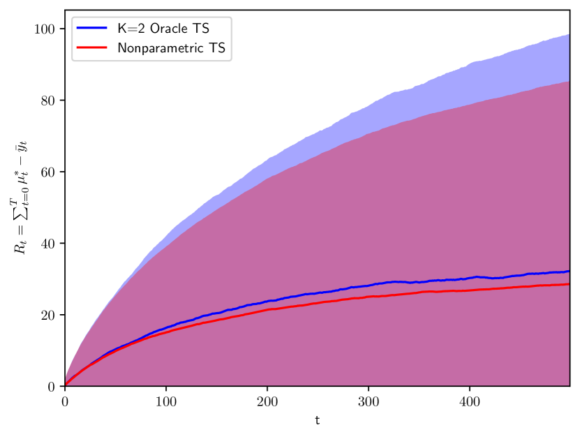
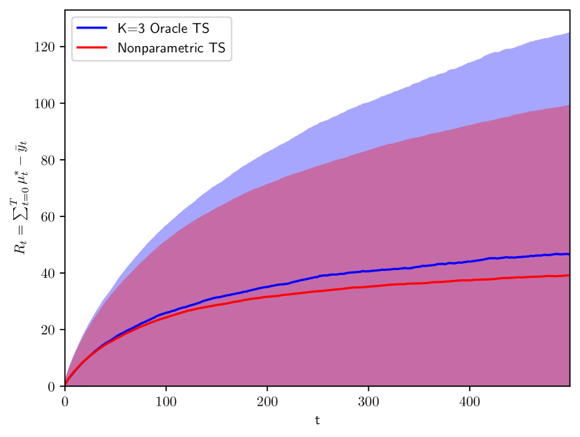
4.3.2 Comparison to Oracle TS
We implement separate Oracle TS algorithms for Scenarios A and B, where the Oracle TS has knowledge of the true underlying complexity per-arm.
To provide a fair comparison, and instead of the variational inference approach proposed by Urteaga and Wiggins (2018) for mixture-model based reward distribution, we implement the Gibbs sampler as described in Algorithm 2 where for each Oracle TS, a Dirichlet prior distribution with the correct per-scenario is known —instead of the Dirichlet process prior of Nonparametric TS.
Figure 7 showcases that Nonparametric TS provides satisfactory performance, when compared to an Oracle TS that knows the true number of underlying mixtures of the problem it is targeted to. Nonparametric TS fits the underlying reward function accurately, attaining regret comparable to the unrealistic Oracle TS. Note that, while per-scenario Oracle TS implementations are needed, Nonparametric TS does not require any per-scenario hyperparameter tuning, yet avoids model misspecification: i.e., the same algorithm is run across all bandit scenarios. These results demonstrate the advantage of BNP models in adjusting the complexity of the reward distribution to the sequentially observed bandit data.
4.4 Contextual heavy-tailed bandits
We now evaluate a bandit scenario of importance in real-life, i.e., one where rewards are subject to outliers. We simulate such scenario as follows:
Wide Gaussian noise (i.e., ) results in per-arm rewards with heavy-tailed distributions. Consequently, the bandit is subject to outlier data that obscures the expected rewards per-arm. We compare Nonparametric TS to baselines in Section 4.4.1 and its corresponding Oracle TS (following the same finite-mixture implementation described above) in Section 4.4.2.
4.4.1 Comparison to baselines
.
of playing the optimal arm.
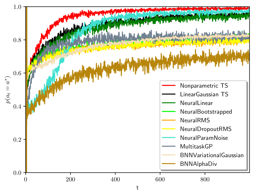
We show in Figure 8(a) how our proposed method attains reduced cumulative regret when compared to all Thompson sampling-based alternatives described in Section 4.1.
Note that most algorithms are not able to find the right exploitation-exploration balance when rewards are subject to outliers: only Nonparametric TS, NeuralParamNoise and LinearGaussian seem to achieve so. However, as seen in Figure 8(b), the proposed algorithm is the fastest in finding the best arm, incurring in less regret.
The flexibility of the nonparametric reward mixture model allows for 30.78% and 42.14% reduction in cumulative regret when compared to the second-best alternatives (NeuralParamNoise and LinearGaussian, respectively), while the rest of the alternatives incur more than double cumulative regret —all results are provided in Table 4.
| Algorithm | Cumulative regret (mean std) | Relative cumulative regret |
|---|---|---|
| Nonparametric TS | 99.972 188.909 | 0.000% |
| LinearGaussian TS | 142.103 200.863 | 42.143% |
| NeuralLinear | 196.797 273.561 | 96.852% |
| NeuralBootstrapped | 214.427 546.000 | 114.487% |
| NeuralRMS | 218.240 556.263 | 118.301% |
| NeuralDropoutRMS | 196.450 510.753 | 96.504% |
| NeuralParamNoise | 130.734 197.637 | 30.771% |
| MultitaskGP | 532.727 310.488 | 432.876% |
| BNNVariationalGaussian | 323.231 691.833 | 223.320% |
| BNNAlphaDiv | 611.635 187.579 | 511.805% |
We again observe unsatisfactory performance of neural network and noise-injection based alternatives: not only on average regret, but on their performance volatility (often twice as of Nonparametric TS). Neural-net based policies struggle to fit the reward distribution appropriately when subject to outliers, resulting in a highly variable performance.
On the contrary, Nonparametric TS is much less volatile, as the BNP posterior allows for accommodating the outlier rewards more flexibly. All in all, Nonparametric TS provides important savings for MAB settings with heavy tailed distributions subject to outliers, where we observe all alternative methods to struggle.
4.4.2 Comparison to Oracle TS
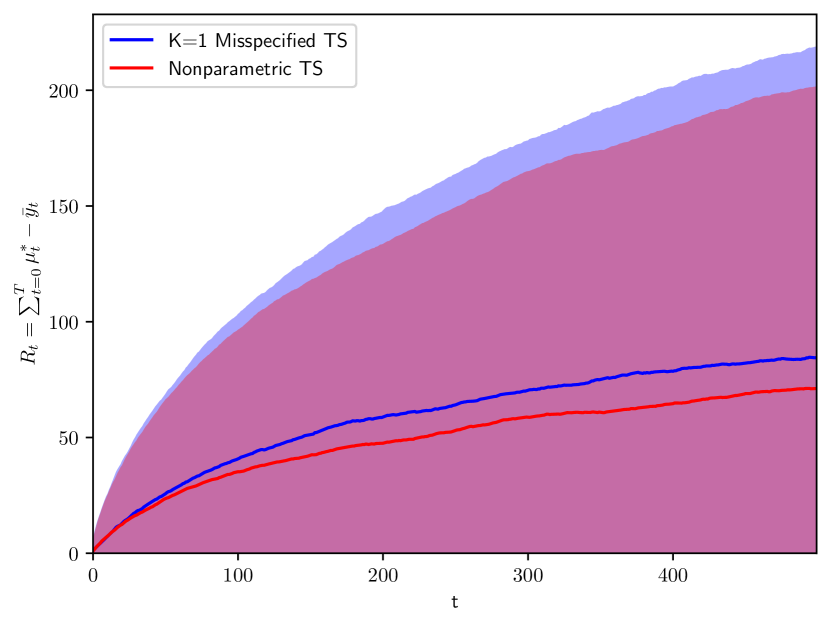
In Figure 9(a), we observe Nonparametric TS policy’s successful performance in the heavy-tailed reward scenario described above: i.e., when compared to an Oracle TS that correctly assumes the number of mixtures () in each per-arm reward distributions.
with knowledge of true model complexity.
under model misspecification.
We highlight the flexibility of the proposed nonparametric Thompson sampling by showing in Figure 9(b) how a misspecified Thompson sampling (i.e., one that fits a unimodal Gaussian distribution to the heavy-tailed reward distributions of this bandit) suffers in comparison to Nonparametric TS: a 18% cumulative regret reduction is attained. The proposed method does not suffer from model misspecification, as it autonomously adapts to the observed rewards, even in the presence of outliers.
4.5 Contextual, exponentially distributed bandits
We scrutinize the flexibility of BNP models to approximate densities with continuous support by evaluating the following exponentially distributed contextual bandit, with rewards constrained to the positive real line, i.e., :
These bandit rewards are contextual not only in expectation, , but in volatility as well: . Because this bandit has not been previously studied and there is no Oracle TS implementation readily available, we focus our evaluation in the comparison of Nonparametric TS to the TS baselines described in Section 4.1.
4.5.1 Comparison to baselines
.
Results in Figure 10 illustrate not only the complexity of this MAB, but also the flexibility and benefits of the nonparametric reward modeling assumption of Nonparametric TS: it is the only policy that finds the optimal arm fastest (see Figure 10(b)), to attain reduced regret.
| Algorithm | Cumulative regret (mean std) | Relative cumulative regret |
|---|---|---|
| Nonparametric TS | 67.860 119.415 | 0.000% |
| LinearGaussian TS | 116.375 129.156 | 71.493% |
| NeuralLinear | 94.192 125.731 | 38.803% |
| NeuralBootstrapped | 138.577 179.869 | 104.210% |
| NeuralRMS | 143.737 173.734 | 111.814% |
| NeuralDropoutRMS | 110.687 173.952 | 63.110% |
| NeuralParamNoise | 146.497 128.506 | 115.881% |
| MultitaskGP | 197.159 140.864 | 190.538% |
| BNNVariationalGaussian | 166.212 227.565 | 144.933% |
| BNNAlphaDiv | 153.459 122.482 | 126.140% |
As detailed in Table 5, all alternative baselines incur considerable additional cumulative regret. These results reinforce our claim that the per-arm BNP posterior converges to the true, unknown (in this case, exponentially distributed) reward distribution, allowing for Nonparametric TS to find the right exploitation-exploration balance, and in turn, achieve reduced regret.
4.6 Evaluation summary and discussion
The proposed Nonparametric TS outperforms state-of-the-art Thompson sampling alternatives across many bandit scenarios, both in averaged cumulative regret, and in regret volatility. It attains reduced regret for reward models not previously studied: Gaussian mixture models, exponentially distributed rewards and rewards subject to outliers, even when there are different model classes per-arm. The competitive advantage lies in the capacity of BNP models to adjust the complexity of the posterior predictive to the sequentially observed bandit data. As such, Nonparametric TS is valuable for bandits in the presence of reward model uncertainty: it avoids case-by-case model design choices. Nonparametric TS can target —without any per-scenario tuning— different MAB settings, and attain significant regret reductions.
As per-arm BNP posteriors converge to the true reward distributions, not only regret benefits are attained, but explainability is enabled: the generative modeling provides per-arm reward understanding, by plotting or computing figures of merit from these distributions. However, recall that posterior convergence does not imply that the BNP model is consistent in the number of mixture components after observations: nonparametric posteriors do not necessarily concentrate at the true number of components on a dataset drawn from a finite mixture model (Miller and Harrison, 2014). We here use BNP mixture models as flexible priors on distributions with guarantees that their posterior converges to the true data generating density, which suffices in the bandit setting for attaining reduced regret.
We observe unsatisfactory performance of neural network-based and approximate Bayesian inference-based Thompson sampling alternatives. They attain poor exploration-exploitation tradeoff and high-volatility in their performance, and there is no clear best alternative across all the studied bandit scenarios. We find that NeuralLinear TS incurs significant additional regret when compared to Nonparametric TS in bandits with reward functions not in the exponential family: additional 107.63% and 77% regret in Scenarios A and B respectively, and 96.85% in the heavy-tailed one. In addition, the volatility of the evaluated neural network based policies is worrisome. For the application of bandits in real-life, the variance of an algorithm’s performance is critical: even if expected reward guarantees are in place, the understanding of how volatile a bandit agent’s decisions are has undeniable real-world impact. On the contrary, the performance of Nonparametric TS is much less volatile, and on par with the (unrealistic) Oracle TS.
Variational inference and expectation-propagation based algorithms also perform poorly in all the studied bandits. While optimizing until convergence at every interaction with the world incurs increased computational cost, our results suggest that it may not be sufficient to optimize the variational parameters in bandit settings. Similarly, for Black-Box -divergence, partial optimization convergence may be the cause of poor regret performance.
Bootstrapped and RMS based neural Thompson sampling techniques struggle to find a good exploration-exploitation balance as well, incurring in additional and very volatile regret performance. As noted by Riquelme et al. (2018), noise injection, bootstrapping and dropout algorithms heavily depend on their hyperparameters, and it is unclear how to disentangle better training from better exploration in these models. On the contrary, Nonparametric TS achieves reduced regret across all scenarios without any case-specific fine-tuning.
Alternative BNP methods, such as those based on Gaussian processes, suffer when the studied scenarios are not unimodal. We argue that such poor performance is explained by model misspecification: Gaussian process regression requires knowledge of the true underlying model class (i.e., what mean and kernel functions to use) —if the reward model class of the MAB they are targeting is not correctly specified, then increased regret is attained. Note that Nonparametric TS requires no per-MAB fine-tuning (we report the effect in bandit regret of different Dirichlet concentration hyperparameters in Section F of the Appendix).
Finally, when computational constraints are appropriate for real-time bandits, limiting the number of Gibbs iterations as presented and discussed in Section 3.2.2 is possible and beneficial. It allows for a drastic reduction in the execution-time of Nonparametric-TS (see results in Section G of the Appendix), while achieving satisfactory cumulative regret: empirical results for different values are provided in Section E of the Appendix.
5 Conclusion
We contribute to the field of sequential decision making by presenting a Bayesian nonparametric mixture model based Thompson sampling that attains reduced regret under reward model uncertainty. We merge advances in the field of Bayesian nonparametric models with a state-of-the art MAB policy, allowing for its extension to complex, previously elusive multi-armed bandit domains. The proposed Bayesian nonparametric Thompson sampling provides flexible modeling of continuous reward functions with convergence guarantees, and attains successful exploration-exploitation trade-off in complex MABs with minimal assumptions. To the best of our knowledge, Nonparametric TS is the first method to successfully operate, without any fine-tuning, in bandits with different per-arm continuous reward distributions, not necessarily in the exponential family.
We provide an asymptotic upper bound for the expected cumulative regret of the proposed Dirichlet process Gaussian mixture model based Thompson sampling. To do so, we introduce a posterior convergence-based analysis, which is conceptually simple yet general enough to be applied to other reward distributions. Our analysis constitutes a first step towards establishing regret bounds for more general BNP process-based reward models.
Empirical results show improved cumulative regret performance of Nonparametric TS, remarkably adjusting to the complexity of the underlying bandit in an online fashion —bypassing model misspecification and hyperparameter tuning— in challenging domains. Important savings are attained for complex bandit settings (e.g., with exponential, mixture model, or heavy tailed reward distributions) where alternative methods struggle. With the ability to sequentially learn the BNP mixture model that best approximates the true reward distribution, Nonparametric TS can be readily applied to diverse MAB settings without stringent model specifications.
Several research endeavors spring out of this work, both theoretical and empirical. On the one hand, research on tightening the presented regret bound and extending it to the more general Pitman-Yor process awaits. As novel nonparametric prior-based posterior convergence results are established Scricciolo (2014) it will be possible to extend the presented regret analysis to other Bayesian nonparametric models: e.g., for normalized inverse-Gaussian processes, or the Poisson-Kingman and the Gibbs partitions (Jang et al., 2010). On the other, evaluation of the benefits and drawbacks of other state-of-the-art inference approaches for Bayesian nonparametric models remains, as well as to apply the proposed method to real-life MAB applications where complex models are likely to outperform simpler ones. A separate research direction relates to the theoretical and practical study of the hierarchical Bayesian nonparametric model presented in Section A of the Appendix (suitable when bandit arms are correlated or dependent) and its connection to multi-task learning: learning about a bandit arm (i.e., task) may help in learning about other arms (i.e., solving similar tasks).
Funding
IU and CHW are supported by the US National Science Foundation Award #1344668.
Conflict of interest
The authors declare that they have no conflict of interest.
References
- Agrawal and Goyal [2012] S. Agrawal and N. Goyal. Analysis of Thompson Sampling for the multi-armed bandit problem. In Conference on Learning Theory, pages 39–1, 2012.
- Agrawal and Goyal [2013a] S. Agrawal and N. Goyal. Further Optimal Regret Bounds for Thompson Sampling. In Artificial Intelligence and Statistics, pages 99–107, 2013a.
- Agrawal and Goyal [2013b] S. Agrawal and N. Goyal. Thompson Sampling for Contextual Bandits with Linear Payoffs. In International Conference on Machine Learning, pages 127–135, 2013b.
- Antoniak [1974] C. E. Antoniak. Mixtures of Dirichlet processes with applications to Bayesian nonparametric problems. The annals of statistics, pages 1152–1174, 1974.
- Aziz et al. [2021] M. Aziz, E. Kaufmann, and M.-K. Riviere. On Multi-Armed Bandit Designs for Dose-Finding Trials. Journal of Machine Learning Research, 22(14):1–38, 2021. URL http://jmlr.org/papers/v22/19-228.html.
- Battiston et al. [2018] M. Battiston, S. Favaro, and Y. W. Teh. Multi-Armed Bandit for Species Discovery: A Bayesian Nonparametric Approach. Journal of the American Statistical Association, 113(521):455–466, 2018. doi: 10.1080/01621459.2016.1261711. URL https://doi.org/10.1080/01621459.2016.1261711.
- Bhattacharya and Dunson [2010] A. Bhattacharya and D. B. Dunson. Nonparametric Bayesian density estimation on manifolds with applications to planar shapes. Biometrika, 97(4):851–865, 2010.
- Blackwell and MacQueen [1973] D. Blackwell and J. B. MacQueen. Ferguson distributions via Pólya urn schemes. The annals of statistics, 1(2):353–355, 1973.
- Blei and Jordan [2004] D. M. Blei and M. I. Jordan. Variational Methods for the Dirichlet Process. In Proceedings of the Twenty-first International Conference on Machine Learning, ICML ’04, pages 12–, New York, NY, USA, 2004. ACM. ISBN 1-58113-838-5. doi: 10.1145/1015330.1015439.
- Blundell et al. [2015] C. Blundell, J. Cornebise, K. Kavukcuoglu, and D. Wierstra. Weight Uncertainty in Neural Networks. In Proceedings of the 32Nd International Conference on International Conference on Machine Learning - Volume 37, ICML’15, pages 1613–1622. JMLR.org, 2015.
- Bubeck and Liu [2013] S. Bubeck and C.-Y. Liu. Prior-free and prior-dependent regret bounds for Thompson Sampling. In C. J. C. Burges, L. Bottou, M. Welling, Z. Ghahramani, and K. Q. Weinberger, editors, Advances in Neural Information Processing Systems 26, pages 638–646. Curran Associates, Inc., 2013. URL http://papers.nips.cc/paper/5108-prior-free-and-prior-dependent-regret-bounds-for-thompson-sampling.pdf.
- Buntine and Hutter [2010] W. Buntine and M. Hutter. A Bayesian view of the Poisson-Dirichlet process. arXiv preprint arXiv:1007.0296, 2010.
- Burnetas and Katehakis [1997] A. N. Burnetas and M. N. Katehakis. Optimal Adaptive Policies for Markov Decision Processes. Mathematics of Operations Research, 22(1):222–255, 1997. doi: 10.1287/moor.22.1.222.
- Camerlenghi et al. [2020] F. Camerlenghi, B. Dumitrascu, F. Ferrari, B. E. Engelhardt, and S. Favaro. Nonparametric Bayesian multi-armed bandits for single-cell experiment design. The Annals of Applied Statistics, 14(4):2003 – 2019, 2020. doi: 10.1214/20-AOAS1370. URL https://doi.org/10.1214/20-AOAS1370.
- Eckles and Kaptein [2019] D. Eckles and M. Kaptein. Bootstrap Thompson Sampling and Sequential Decision Problems in the Behavioral Sciences. SAGE Open, 9(2):2158244019851675, 2019. doi: 10.1177/2158244019851675. URL https://doi.org/10.1177/2158244019851675.
- Escobar and West [1995] M. D. Escobar and M. West. Bayesian density estimation and inference using mixtures. Journal of the American statistical association, 90(430):577–588, 1995.
- Fearnhead [2004] P. Fearnhead. Particle filters for mixture models with an unknown number of components. Statistics and Computing, 14(1):11–21, 2004.
- Ferguson [1973] T. S. Ferguson. A Bayesian analysis of some nonparametric problems. The annals of statistics, pages 209–230, 1973.
- Gershman and Blei [2012] S. J. Gershman and D. M. Blei. A tutorial on Bayesian nonparametric models. Journal of Mathematical Psychology, 56(1):1 – 12, 2012. ISSN 0022-2496. doi: https://doi.org/10.1016/j.jmp.2011.08.004.
- Ghosal [2010] S. Ghosal. The Dirichlet process, related priors and posterior asymptotics. Bayesian nonparametrics, 28:35, 2010.
- Ghosal and der Vaart [2017] S. Ghosal and A. V. der Vaart. Fundamentals of nonparametric Bayesian inference, volume 44. Cambridge University Press, 2017.
- Ghosal and van der Vaart [2007] S. Ghosal and A. van der Vaart. Posterior convergence rates of Dirichlet mixtures at smooth densities. Ann. Statist., 35(2):697–723, 04 2007. doi: 10.1214/009053606000001271.
- Ghosal and van der Vaart [2001] S. Ghosal and A. W. van der Vaart. Entropies and rates of convergence for maximum likelihood and Bayes estimation for mixtures of normal densities. Ann. Statist., 29(5):1233–1263, 10 2001. doi: 10.1214/aos/1013203452. URL https://doi.org/10.1214/aos/1013203452.
- Ghosal et al. [1999] S. Ghosal, J. K. Ghosh, and R. Ramamoorthi. Posterior consistency of Dirichlet mixtures in density estimation. Annals of Statistics, 27(1):143–158, 1999. URL http://repository.ias.ac.in/22510/1/308.pdf.
- Ghosal et al. [2000] S. Ghosal, J. K. Ghosh, and A. W. van der Vaart. Convergence rates of posterior distributions. Ann. Statist., 28(2):500–531, 04 2000. doi: 10.1214/aos/1016218228. URL https://doi.org/10.1214/aos/1016218228.
- Gopalan and Mannor [2015] A. Gopalan and S. Mannor. Thompson Sampling for Learning Parameterized Markov Decision Processes. In P. Grünwald, E. Hazan, and S. Kale, editors, Proceedings of The 28th Conference on Learning Theory, volume 40 of Proceedings of Machine Learning Research, pages 861–898, Paris, France, 03–06 Jul 2015. PMLR. URL http://proceedings.mlr.press/v40/Gopalan15.html.
- Grünewälder et al. [2010] S. Grünewälder, J.-Y. Audibert, M. Opper, and J. Shawe-Taylor. Regret Bounds for Gaussian Process Bandit Problems. In Y. W. Teh and M. Titterington, editors, Proceedings of the Thirteenth International Conference on Artificial Intelligence and Statistics, volume 9 of Proceedings of Machine Learning Research, pages 273–280, Chia Laguna Resort, Sardinia, Italy, 13–15 May 2010. PMLR. URL http://proceedings.mlr.press/v9/grunewalder10a.html.
- Hernandez-Lobato et al. [2016] J. Hernandez-Lobato, Y. Li, M. Rowland, T. Bui, D. Hernandez-Lobato, and R. Turner. Black-box alpha divergence minimization. In M. F. Balcan and K. Q. Weinberger, editors, Proceedings of The 33rd International Conference on Machine Learning,, volume 48 of Proceedings of Machine Learning Research, pages 1511–1520, New York, New York, USA, 20–22 Jun 2016. PMLR. URL http://proceedings.mlr.press/v48/hernandez-lobatob16.html.
- Hill et al. [2017] D. N. Hill, H. Nassif, Y. Liu, A. Iyer, and S. Vishwanathan. An efficient bandit algorithm for realtime multivariate optimization. In Proceedings of the 23rd ACM SIGKDD International Conference on Knowledge Discovery and Data Mining, pages 1813–1821. ACM, 2017.
- Hjort et al. [2010] N. L. Hjort, C. Holmes, P. Müller, and S. G. Walker. Bayesian nonparametrics, volume 28. Cambridge University Press, 2010.
- Ibragimov and Has’minskii [1981] I. Ibragimov and R. Has’minskii. Statistical Estimation: Asymptotic Theory. Springer, 1981. doi: 10.1007/978-1-4899-0027-2.
- Ishwaran and James [2001] H. Ishwaran and L. F. James. Gibbs Sampling Methods for Stick-Breaking Priors. Journal of the American Statistical Association, 96(453):161–173, 2001. doi: 10.1198/016214501750332758. URL https://doi.org/10.1198/016214501750332758.
- Jang et al. [2010] G. H. Jang, J. Lee, and S. Lee. Posterior consistency of species sampling priors. Statistica Sinica, pages 581–593, 2010.
- Kingma et al. [2015] D. P. Kingma, T. Salimans, and M. Welling. Variational Dropout and the Local Reparameterization Trick. In C. Cortes, N. D. Lawrence, D. D. Lee, M. Sugiyama, and R. Garnett, editors, Advances in Neural Information Processing Systems 28, pages 2575–2583. Curran Associates, Inc., 2015.
- Korda et al. [2013] N. Korda, E. Kaufmann, and R. Munos. Thompson Sampling for 1-Dimensional Exponential Family Bandits. In C. J. C. Burges, L. Bottou, M. Welling, Z. Ghahramani, and K. Q. Weinberger, editors, Advances in Neural Information Processing Systems 26, pages 1448–1456. Curran Associates, Inc., 2013.
- Krause and Ong [2011] A. Krause and C. S. Ong. Contextual Gaussian Process Bandit Optimization. In J. Shawe-Taylor, R. S. Zemel, P. L. Bartlett, F. Pereira, and K. Q. Weinberger, editors, Advances in Neural Information Processing Systems 24, pages 2447–2455. Curran Associates, Inc., 2011.
- Lai and Robbins [1985] T. L. Lai and H. Robbins. Asymptotically Efficient Adaptive Allocation Rules. Advances in Applied Mathematics, 6(1):4–22, mar 1985. ISSN 0196-8858. doi: 10.1016/0196-8858(85)90002-8.
- Lattimore and Szepesvári [2020] T. Lattimore and C. Szepesvári. Bandit algorithms. Cambridge University Press, 2020.
- Li et al. [2016] C. Li, C. Chen, D. Carlson, and L. Carin. Preconditioned Stochastic Gradient Langevin Dynamics for Deep Neural Networks. In Proceedings of the Thirtieth AAAI Conference on Artificial Intelligence, AAAI’16, pages 1788–1794. AAAI Press, 2016.
- Li et al. [2010] L. Li, W. Chu, J. Langford, and R. E. Schapire. A Contextual-Bandit Approach to Personalized News Article Recommendation. In Proceedings of the 19th international conference on World wide web, volume abs/1003.0146, pages 661–670, 2010.
- Lijoi et al. [2004] A. Lijoi, I. Prünster, and S. G. Walker. Extending Doob’s consistency theorem to nonparametric densities. Bernoulli, 10(4):651–663, 2004.
- Lipton et al. [2018] Z. C. Lipton, X. Li, J. Gao, L. Li, F. Ahmed, and L. Deng. BBQ-Networks: Efficient Exploration in Deep Reinforcement Learning for Task-Oriented Dialogue Systems. In AAAI, 2018.
- Lu and Roy [2017] X. Lu and B. V. Roy. Ensemble sampling. In Advances in Neural Information Processing Systems, pages 3258–3266, 2017.
- Mauldin et al. [1992] R. D. Mauldin, W. D. Sudderth, and S. C. Williams. Polya trees and random distributions. The Annals of Statistics, pages 1203–1221, 1992.
- Miller and Harrison [2014] J. W. Miller and M. T. Harrison. Inconsistency of Pitman-Yor Process Mixtures for the Number of Components. Journal of Machine Learning Research, 15:3333–3370, 2014. URL http://jmlr.org/papers/v15/miller14a.html.
- Müller et al. [2015] P. Müller, F. A. Quintana, A. Jara, and T. Hanson. Bayesian nonparametric data analysis. Springer, 2015. doi: 10.1007/978-3-319-18968-0.
- Neal [2000] R. M. Neal. Markov Chain Sampling Methods for Dirichlet Process Mixture Models. Journal of Computational and Graphical Statistics, 9(2):249–265, 2000. ISSN 10618600.
- Osband and Roy [2015] I. Osband and B. V. Roy. Bootstrapped Thompson sampling and deep exploration. arXiv preprint arXiv:1507.00300, 2015.
- Osband et al. [2016] I. Osband, C. Blundell, A. Pritzel, and B. V. Roy. Deep Exploration via Bootstrapped DQN. In D. D. Lee, M. Sugiyama, U. V. Luxburg, I. Guyon, and R. Garnett, editors, Advances in Neural Information Processing Systems 29, pages 4026–4034. Curran Associates, Inc., 2016.
- Ouyang et al. [2017] Y. Ouyang, M. Gagrani, A. Nayyar, and R. Jain. Learning Unknown Markov Decision Processes: A Thompson Sampling Approach. In I. Guyon, U. V. Luxburg, S. Bengio, H. Wallach, R. Fergus, S. Vishwanathan, and R. Garnett, editors, Advances in Neural Information Processing Systems 30, pages 1333–1342. Curran Associates, Inc., 2017. URL http://papers.nips.cc/paper/6732-learning-unknown-markov-decision-processes-a-thompson-sampling-approach.pdf.
- Pati et al. [2013] D. Pati, D. B. Dunson, and S. T. Tokdar. Posterior consistency in conditional distribution estimation. Journal of multivariate analysis, 116:456–472, 2013.
- Pitman and Yor [1997] J. Pitman and M. Yor. The two-parameter Poisson-Dirichlet distribution derived from a stable subordinator. The Annals of Probability, 25(2):855 – 900, 1997. doi: 10.1214/aop/1024404422. URL https://doi.org/10.1214/aop/1024404422.
- Plappert et al. [2018] M. Plappert, R. Houthooft, P. Dhariwal, S. Sidor, R. Y. Chen, X. Chen, T. Asfour, P. Abbeel, and M. Andrychowicz. Parameter Space Noise for Exploration. In International Conference on Learning Representations, 2018.
- Rasmussen and Williams [2005] C. E. Rasmussen and C. K. I. Williams. Gaussian Processes for Machine Learning. The MIT Press, 2005.
- Rindtorff et al. [2019] N. T. Rindtorff, M. Lu, N. A. Patel, H. Zheng, and A. D’Amour. A biologically plausible benchmark for contextual bandit algorithms in precision oncology using in vitro data. arXiv preprint arXiv:1911.04389, 2019.
- Riquelme et al. [2018] C. Riquelme, G. Tucker, and J. Snoek. Deep Bayesian Bandits Showdown: An Empirical Comparison of Bayesian Deep Networks for Thompson Sampling. In International Conference on Learning Representations, 2018.
- Robbins [1952] H. Robbins. Some aspects of the sequential design of experiments. Bulletin of the American Mathematical Society, (58):527–535, 1952.
- Russo and Roy [2014] D. Russo and B. V. Roy. Learning to optimize via posterior sampling. Mathematics of Operations Research, 39(4):1221–1243, 2014.
- Russo and Roy [2016] D. Russo and B. V. Roy. An information-theoretic analysis of Thompson sampling. The Journal of Machine Learning Research, 17(1):2442–2471, 2016.
- Russo et al. [2018] D. J. Russo, B. V. Roy, A. Kazerouni, I. Osband, and Z. Wen. A Tutorial on Thompson Sampling. Foundations and Trends® in Machine Learning, 11(1):1–96, 2018. ISSN 1935-8237. doi: 10.1561/2200000070. URL http://dx.doi.org/10.1561/2200000070.
- Scricciolo [2014] C. Scricciolo. Adaptive Bayesian density estimation in Lp-metrics with Pitman-Yor or normalized inverse-Gaussian process kernel mixtures. Bayesian Analysis, 9(2):475–520, 2014.
- Sethuraman [1994] J. Sethuraman. A constructive definition of Dirichlet priors. Statistica sinica, pages 639–650, 1994.
- Slivkins [2019] A. Slivkins. Introduction to Multi-Armed Bandits. Foundations and Trends in Machine Learning, 12(1-2):1–286, 2019. ISSN 1935-8237. doi: 10.1561/2200000068. URL http://dx.doi.org/10.1561/2200000068.
- Srinivas et al. [2010] N. Srinivas, A. Krause, S. Kakade, and M. Seeger. Gaussian Process Optimization in the Bandit Setting: No Regret and Experimental Design. In Proceedings of the 27th International Conference on International Conference on Machine Learning, ICML’10, pages 1015–1022, USA, 2010. Omnipress. ISBN 978-1-60558-907-7.
- Teh and Jordan [2010] Y. W. Teh and M. I. Jordan. Hierarchical Bayesian nonparametric models with applications. Bayesian nonparametrics, 1:158–207, 2010.
- Teh et al. [2006] Y. W. Teh, M. I. Jordan, M. J. Beal, and D. M. Blei. Hierarchical Dirichlet Processes. Journal of the American Statistical Association, 101(476):1566–1581, 2006. doi: 10.1198/016214506000000302.
- Thompson [1933] W. R. Thompson. On the Likelihood that One Unknown Probability Exceeds Another in View of the Evidence of Two Samples. Biometrika, 25(3/4):285–294, 1933. ISSN 00063444.
- Thompson [1935] W. R. Thompson. On the Theory of Apportionment. American Journal of Mathematics, 57(2):450–456, 1935. ISSN 00029327, 10806377.
- Tokdar [2006] S. T. Tokdar. Posterior consistency of Dirichlet location-scale mixture of normals in density estimation and regression. Sankhyā: The Indian Journal of Statistics, pages 90–110, 2006.
- Urteaga and Wiggins [2018] I. Urteaga and C. Wiggins. Variational inference for the multi-armed contextual bandit. In A. Storkey and F. Perez-Cruz, editors, Proceedings of the Twenty-First International Conference on Artificial Intelligence and Statistics, volume 84 of Proceedings of Machine Learning Research, pages 698–706, Playa Blanca, Lanzarote, Canary Islands, 09–11 Apr 2018. PMLR.
- Villar et al. [2015] S. S. Villar, J. Bowden, and J. Wason. Multi-armed Bandit Models for the Optimal Design of Clinical Trials: Benefits and Challenges. Statistical Science, 30(2):199 – 215, 2015. doi: 10.1214/14-STS504. URL https://doi.org/10.1214/14-STS504.
Appendix A Nonparametric hierarchical mixture model bandit
An alternative nonparametric MAB model is to consider a hierarchical Dirichlet Process (or Pitman-Yor) mixture model [Teh and Jordan, 2010] where each arm’s random reward distribution is drawn from the same, shared across arms, base measure.
The generative process of a hierarchical Pitman-Yor mixture model follows:
| (37) | ||||
| (38) | ||||
| (39) | ||||
| (40) |
In this model, illustrated in Figure 11, because all arms of the bandit belong to the same family of reward distributions , rewards observed from the distribution of a particular bandit arm allow learning about other arms’ distributions. Note that the hierarchical Dirichlet process is a particular case of the presented model with .
Hierarchical modeling rationale.
The hierarchical BNP model above defines, due to the clustering properties of the DP and PY processes, a global mixture with distinct components or “atoms” for the bandit, which may (or may not) appear with different probabilities across arms: i.e., the same distinct s are shared across arms, with only mixture proportions varying across arms.
Specifically, let us denote with the per-arm assignments to unique local (per-arm) mixture components , . Each of these is associated with global mixtures , now shared across arms: i.e., is number of local mixture components assigned to global mixture component , and . That is, there is a global mixture with “atoms” for the bandit, but each per-arm distribution consists of a subset of mixture components. We refer the interested reader on hierarchical DP and PY processes to [Teh and Jordan, 2010].
The main advantage of this alternative is that one learns per-mixture parameter posteriors based on rewards of all played arms, with the disadvantage of all arms of the bandit being of the same family of reward distributions.
Inference of the model.
The Gibbs sampler for inference of the above model after observations relies on the conditional distribution of observation assignments to local mixture components ,
| (41) |
with mixture assignments for distinct local mixture components ,
| (42) |
and a potential new mixture component
| (43) |
where refers to all observations assigned to local component in arm , are the number of local mixture components assigned to global mixture component , and .
We again write and for parametric base measures, where are the prior hyperparameters of the emission distribution, and the posterior parameters after observations, respectively. If the base measure is conjugate to the emission distribution , analytical posteriors and collapsed Gibbs sampler steps can be derived, analogous to those provided in Section C for the non-hierarchical case.
Appendix B Asymptotic regret bound for Bayesian nonparametric mixture model based Thompson sampling
We start by clarifying the notation we use in the sequel:
-
•
The distribution of the random variable denotes the probability of a random event with .
-
•
We specify the distribution of the random variable within an expectation with a subscript, .
-
•
We use to indicate the expectation under some distribution of the reward for each arm .
-
•
We use for the sequence of all per-arm expected values.
-
•
We define the union of the context at time and history up to with .
-
•
We use to indicate the expectation under the posterior of the reward distribution of each arm given context and history up to time .
-
•
We denote stochastic policies with , where the subscript makes explicit the assumed reward model class .
-
•
For Thompson sampling policies, we may interchangeably write
(44) -
•
The total variation distance between distributions and on a sigma-algebra of subsets of the sample space is defined as
(45) When is countable,
(46) which is directly related to the norm
(47) More broadly, if and are both absolutely continuous with respect to some base measure ,
(48) where and are the Radon-Nikodym derivatives of and with respect to .
We now re-state and prove Lemma 3.1:
Lemma 3.1: The difference in action probabilities between two Thompson sampling policies under reward distributions and , given the same history and context up to time , is bounded by the total-variation distance between the posterior distributions of their expected rewards at time , and , respectively:
| (49) |
The proof of Lemma 3.1 consists of showing that the difference between the expected values of a function of a random variable is bounded by the total variation distance between the corresponding distributions.
Proof.
Let us define a linear function of a bounded function :
| (50) |
Then,
| (51) |
We now recall that we can write the difference between two Thompson sampling policies as
| (52) |
Let us define , which is bounded in :
| (53) |
Direct substitution in Equation (51) results in
| (54) |
which concludes the proof. ∎
We make use of Lemma 3.1 to bound the asymptotic expected cumulative regret of the proposed Thompson sampling with a Dirichlet process mixture prior. To that end, let us define the following Thompson sampling policies:
-
•
The optimal Thompson sampling policy, , which chooses the optimal arm given the true reward model ,
(55) -
•
A parametric, Oracle Thompson sampling policy, , which knows the true reward distribution model class , but not the true parameter ,
(56) The actions of this Thompson sampling policy, denoted as , are stochastic due to the uncertainty on the parameter of the true density .
-
•
A BNP Thompson sampling policy, , which estimates the unknown true reward distribution with a BNP mixture model ,
(57) The actions of this Thompson sampling policy, denoted as , are stochastic due to the uncertainty on the parameter of the BNP distribution .
Theorem 3.2: The expected cumulative regret at time of a Dirichlet process Gaussian mixture model based Thompson sampling algorithm is, for , asymptotically bounded by
| (58) |
where the expectations are taken over the random rewards and the random actions of the stochastic policies and .
This expected regret bound holds in the frequentist sense, and the logarithmic term appears due to the convergence rate of the BNP posterior, where the exponent depends on the tail behavior of the base measure and the priors of the Dirichlet process [Ghosal and van der Vaart, 2001].
We use big-O notation as it bounds from above the growth of the cumulative regret over time for large enough input sizes, i.e.,
| (59) |
In the following, we avoid notation clutter and denote for the true reward distribution given the true parameters , and drop the dependency over the observed history at time in the considered Thompson sampling policies.
We write, , for the optimal Thompson sampling policy with knowledge of the true reward model ; , for an Oracle Thompson sampling policy with knowledge of the true reward distribution model class —but not the true parameter ; and , for a BNP Thompson sampling policy that estimates the unknown true reward distribution with a BNP model .
Proof.
| (60) | ||||
| (61) | ||||
| (62) | ||||
| (63) | ||||
| (64) | ||||
| (65) |
where we have split the expected cumulative regret of Equation 60 in two terms.
The first term in the RHS of Equation 65 relates to the regret between the optimal policy and an Oracle Thompson sampling policy that knows the true model class ; and the second term in the RHS of Equation 65 accommodates the regret between the Oracle Thompson sampling policy that knows the true model class , and a nonparametric Thompson sampling that estimates reward functions via BNP models .
Let us first work on the first term in the RHS of Equation 65:
| (66) | |||
| (67) | |||
| (68) | |||
| (69) | |||
| (70) | |||
| (71) | |||
| (72) | |||
| (73) | |||
| (74) | |||
| (75) | |||
| (76) |
where
-
•
in Equation 70: we define , i.e., it is an upper bound on the expected rewards of the bandit.
-
•
in Equation 71: by direct application of Equation 49 in Lemma 3.1:
.That is, the difference in probabilities of playing each arm are bounded by the total variation distance between the posterior distributions of the expected rewards for each policy.
For the optimal Thompson sampling policy, the parameters of the reward distribution are known, i.e., the posterior is a delta at the true value:
For the Thompson sampling policy that knows the true model class, the parameters of the reward distribution are updated as history is observed, via its posterior distribution ,
-
•
in Equation 72: , as , where is a constant that depends on the properties of the parameterized distributions, and does not depend on the amount of observed data.
As explained in [Ghosal et al., 2000], for a class of parameterized distributions and a prior constructed by putting a measure on the parameter set , it is well known that the posterior distribution of asymptotically achieves the optimal rate of convergence under mild regularity conditions —i.e., is a subset of a finite-dimensional Euclidean space, and the prior and model dependence is sufficiently regular [Ibragimov and Has’minskii, 1981]. In particular, and according to the Bernstein-von Mises theorem, if the model is suitably differentiable, then the convergence rate of the posterior mean and is of order , where indicates the amount of i.i.d. data drawn from the true distribution .Note that the true and the posterior are over the expected rewards of all arms. Therefore, , where indicates the number of observations for each arm, is the number of times all arms have been pulled. Consequently, the total variation Equation 72 depends on the total number of observations across all arms .
-
•
in Equation 74: , where is the generalized harmonic number of order of .
This concludes the proof of the bound of the first term in the RHS of Equation 65. We now bound the second term in the RHS:
| (77) | |||
| (78) | |||
| (79) | |||
| (80) | |||
| (81) | |||
| (82) | |||
| (83) | |||
| (84) | |||
| (85) | |||
| (86) | |||
| (87) |
where
-
•
in Equation 81: , as above.
-
•
in Equation 82: by direct application of Equation 49 in Lemma 3.1:
.That is, the difference in probabilities of playing each arm are bounded by the total variation distance between the posterior distributions of the expected rewards for each policy.
For the Thompson sampling policy that knows the true model class, the parameters of the reward distribution are updated as history is observed:
For the Thompson sampling that estimates reward functions via BNP model , the parameters of the nonparametric reward distribution are updated as history is observed:
-
•
in Equation 83: , as ; where is a constant that depends on the properties of both the true parametric posterior distribution and the Bayesian nonparametric prior model, but does not depend on the amount of observed data. Note that the posterior is over the expected rewards over all arms. Therefore, Equation 83 depends on the total number of observations across all arms , where indicates the number of observations observed for each arm .
We asymptotically bound the total variation distance between the true parametric posterior distribution and a BNP model posterior distribution, leveraging state-of-the-art results. Specifically, the work by Ghosal and van der Vaart [2001, 2007] provides posterior convergence rates of Dirichlet process Gaussian mixture models to different distributions. For example, for a mixture of normals with standard deviations bounded by two positive numbers, Ghosal and van der Vaart [2001] show that the Hellinger distance between the BNP posterior given data samples and the true distribution is asymptotically bounded,
(88) where the value depends on the choices of priors over the location and scale of the mixtures, and data is drawn from the true distribution . Since , bounds in Hellinger distance apply to total variation distance as well. Note that the convergence of the posterior at such a rate also implies that there exist estimators, such as the posterior mean, that converge at the same rate in the frequentist sense.
Technical details on the tightness of the bound in Equation (88) can be found in [Ghosal and van der Vaart, 2001]. For instance, a rate with is obtained when a compactly supported base measure is used for the location prior (and the scale prior has a continuous and positive density on an interval containing the true scale parameter). For the commonly used normal base measure, the bound yields a rate . When the base measure is the product of a normal distribution with a distribution supported within the range of the true scale, such that the density is positive on a rectangle containing the true location-scale space, the rate results in .
Later work by Ghosal and van der Vaart [2007] provides new posterior convergence rates for densities that are twice continuously differentiable, where under some regularity conditions, the posterior distribution based on a Dirichlet mixture of normal prior attains a convergence rate of . As such, it seems reasonable that the power of the logarithm, i.e., in Equation (88), can be improved. Indeed, Ghosal and van der Vaart [2007] argue that, by using a truncated inverse-gamma prior on the scale of the Gaussian mixtures, a nearly optimal convergence rate is obtained —for which one would need to extend the Gibbs sampler with an additional accept-reject step to take care of the scale truncation.
All these bounds would not be directly applicable if the true data generating density would not be part of the model classes considered. However, Ghosal and van der Vaart [2001] argue that a rate for these cases may as well be calculated, but since they may not be close to the optimal rate, have not been pursued yet.
-
•
in Equation 84: .
-
•
in Equation 85, as in Equation 74,: , where is the generalized harmonic number of order of .
Combining the above results, we can now bound the asymptotic cumulative regret in Equation 60, for a nonparametric Thompson sampling policy with Dirichlet process Gaussian mixtures, with priors and data-generating densities that meet the necessary regularity conditions, as follows
| (89) | ||||
| (90) | ||||
| (91) | ||||
| (92) |
This bound holds both in a frequentist and Bayesian view of expected cumulative regret. ∎
Appendix C Details on the Gibbs sampler for per-arm rewards’ DP mixture model posterior
We describe in detail the proposed per-arm posterior Gibbs sampler in Algorithm 2, which is a direct implementation of Algorithm 3 described by Neal [2000].
The Gibbs sampler consists of updating the conditional assignments of each observed reward to its corresponding mixture. To that end, we use auxiliary latent variables that keep track of which distinct mixture component each observation is drawn from. In our case, because we are using independent DP mixture models per-arm, we keep track of per-arm observations and assignments , each of size , for a total of . These are dimensional categorical variables, where for if observation is drawn from arm and mixture component .
We update them via Gibbs sampling using the following conditional probabilities:
| (93) | ||||
| (94) |
Above, is the posterior measure (after observing rewards from arm ) of per-arm parameters assigned to distinct mixtures ; while denotes the prior DP base measure.
The posterior distribution of distinct mixture parameters .
We write for the prior per-arm base measure and for the posterior distribution of distinct per-arm parameters after observing rewards from arm — are the prior hyperparameters, and the posterior hyperparameters.
We compute these posteriors in closed form, due to the conjugacy of per-arm reward emission distributions and base measures considered. They follow a normal inverse-gamma distribution
| (95) |
with hyperparameters
| (96) |
where is a sparse diagonal matrix with elements for . The posterior updates depend on the number of rewards after playing arm that are assigned to mixture component , i.e., .
Marginalized assignment probabilities.
In order to compute the assignment probabilities for the Gibbs sampler, we marginalize out the parameters on the right hand size of Equations (93)–(94), i.e.,
| (97) |
where we use to denote, in general, both the prior and the posterior , depending on whether we are computing the integral with respect to distinct mixture components or a potential new component .
Due to the conjugacy of the emission distribution and —a normal inverse-gamma distribution for both the prior and the posterior— the per-arm reward predictive emission distribution follows a context conditional Student-t distribution
| (98) |
The hyperparameters are computed based on the prior , or the posterior as in Equation (24), depending on whether the predictive density refers to a ‘new’ component with in Equation (94), or a ‘distinct’ already instantiated components in Equation (93), for which observations have been already assigned to, respectively.
The marginalized data likelihood of a set of rewards assigned to per-arm distinct component , , given their associated contexts , (which will be of use below) obeys the following matrix t-distribution
| with | (99) |
Joint marginalized data likelihood.
A key step of the Gibbs sampler is to determine its convergence criteria, for which the joint likelihood of per-arm nonparametric assignments and observations is used. This joint marginalized data likelihood is computed via the following factorization —note that the following applies for PY processes, and we use for DP processes:
| (100) |
where the conditional data-likelihood term
| (101) |
is computed as shown in Equation (99).
The joint posterior of the auxiliary assignment variables factorizes as follows:
| (102) |
which in turn allows for computation of the joint distribution —details can be found in [Buntine and Hutter, 2010]— of the assignments to distinct mixture components per-arm:
| (103) |
above denotes the rising factorial (also known as the Pochhammer function or polynomial), ; and denotes the Pochhammer polynomial with increment : .
Appendix D Non-contextual Gaussian bandits: comparison to Oracle TS
We show in Figure 12 how our proposed nonparametric Thompson sampling method achieves regret comparable to that of the non-contextual Gaussian Thompson sampling as in Agrawal and Goyal [2012], i.e., the Oracle TS, for diverse parameterizations of such Gaussian bandits. Recall that the non-contextual bandit scenario is seamlessly accommodated by our proposed Nonparametric TS algorithm by assuming a constant context, i.e., .
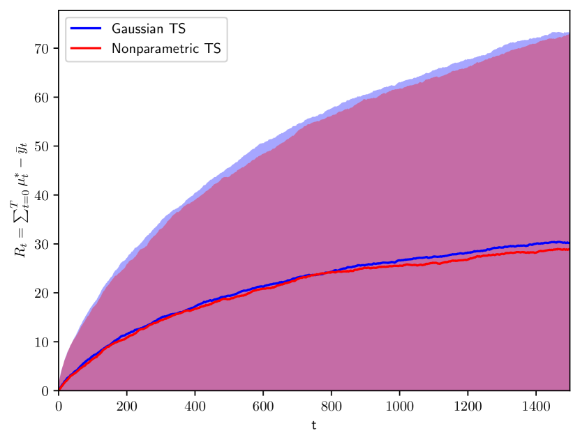
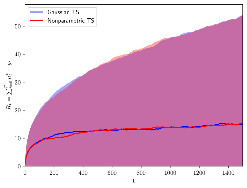
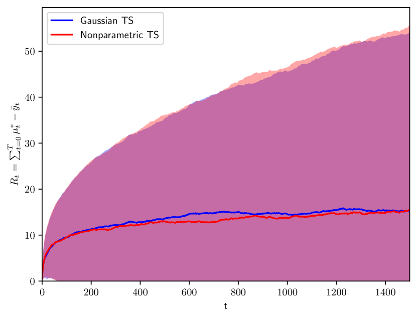
Appendix E Gibbs sampler: computational complexity and regret
We hereby empirically investigate the warm-start effect in the proposed algorithm’s Gibbs sampling procedure, and how the practical recommendations on limiting the number of Gibbs iterations of Section 3.2.2 impact regret performance. In general, and because of the incremental availability of observations in the bandit setting, the proposed Gibbs sampler achieves quick convergence: in all our experiments, a 1% log-likelihood relative difference between iterations is usually achieved within iterations. We show in Figures 13–14 how no significant regret performance improvement is achieved when running Nonparametric TS with or , while we observe that executing only one Gibbs interaction incurs additional regret for exponentially distributed rewards.
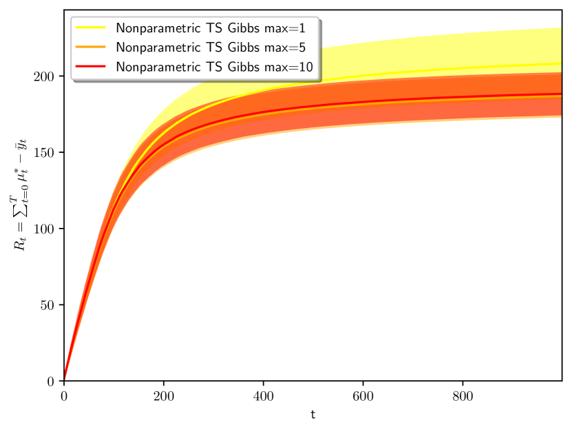
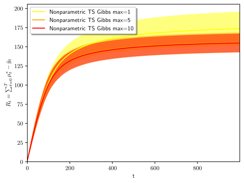
These results support the claim that it is possible to converge to a good enough posterior at a limited computational budget (see the computational benefits of limiting in Figures 17–18). This good enough posterior inference is possible due to the good starting point of the Gibbs sampler at each interaction with the world: the per-arm BPN parameter space that describes all but the newly observed reward. As a result, even if the Gibbs sampler is run for at most updates per interaction, the inferred BNP based model posterior is informative enough to successfully guide the next bandit arm selection.
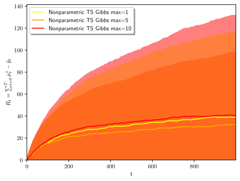
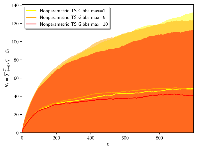
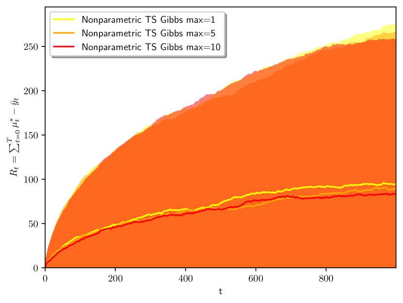
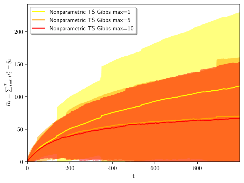
Appendix F Dirichlet process prior hyperparameters:
sparsity and regret
The concentration hyperparameter specifies how sparse a random distribution drawn from a Dirichlet process is: when , the distinct atoms of concentrate at a single value, while in the limit of , the realizations become continuous, as distributed by the base measure .
We empirically investigate the effect that different Dirichlet process priors have, via concentration hyperparameter , in the proposed algorithm’s regret performance. We consider a range of for the Dirichlet process prior in Nonparametric TS, and evaluate the influence of these mixture model sparsity assumptions in the algorithm’s regret.
We demonstrate in Figure 15 how, for a uni-modal density —when true rewards are drawn from a single Gaussian distribution— sparsity inducing priors are (as expected) the best performing algorithms. Note that there are no significant differences between Nonparametric TS run with .
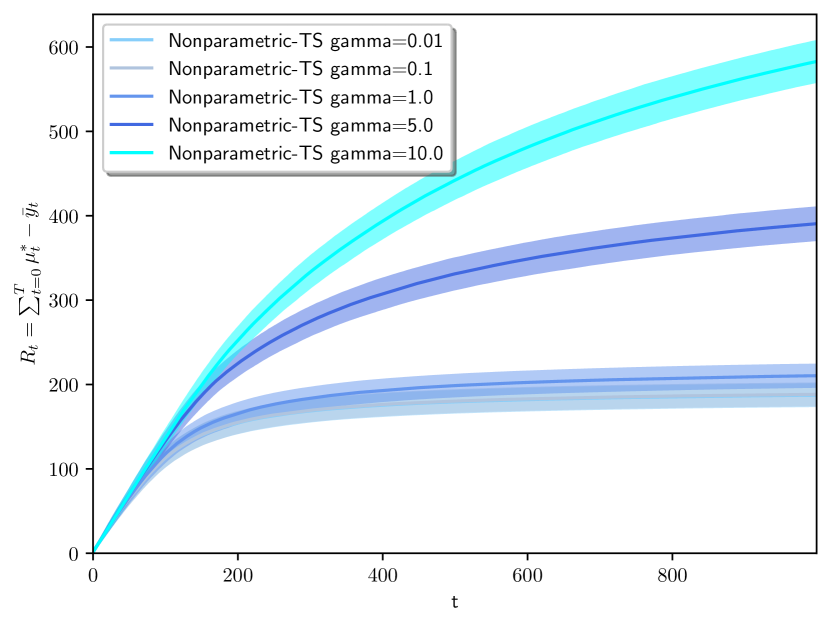
We showcase in Figure 16 how, for mixture-model densities, a less sparsity inducing prior becomes most competitive, while Nonparametric TS with provides a slight performance improvement for bandits with exponentially distributed rewards.
Overall, without prior knowledge of the sparsity of the true reward function and based on the provided empirical evidence, we suggest to use weak sparsity inducing priors, e.g., , as they provide robust and satisfactory performance across the studied bandit scenarios. Incorporating techniques (e.g., resampling steps) that adjust hyperparameter values along with inference of other parameters (e.g., within the proposed Gibbs sampler) is a research direction to be investigated.
Appendix G Computational complexity and run-times of the evaluated Thompson sampling algorithms
Computational cost is an important metric in real-life bandit scenarios, which motivated us to provide a computational analysis of our proposed algorithm in Section 3.2.2. In general, the computational complexity of the proposed algorithm is upper bounded by , which depends on the convergence criteria: i.e., either the model likelihood of the sampled chain is stable within an likelihood margin between iterations, or a maximum number of iterations is reached. As such, tweaking these two values controls the resulting run-times.
We provide below a comparison of the run-times incurred in the set of experiments described in the manuscript, for which we would like to raise two cautionary disclaimers:
-
•
We compare algorithms with different implementations:
The proposed Nonparametric TS is implemented with standard python libraries (i.e., numpy, scipy), while the rest of the algorithms are implemented in Tensorflow, as provided in the Deep Contextual bandit implementation by Riquelme et al. [2018]. Our goal here is to introduce a new bandit algorithm, and improving the efficiency of our implementation is out of the scope of this work. -
•
Our algorithm and those in the deep contextual bandits showdown require updates at every time instant that depend on the number of observations per-arm :
Performance and running-time differences can be achieved if one tweaks each algorithm’s settings for model updates. As explained in Riquelme et al. [2018], a key question is how often and for how long models are updated, as these will determine their running-times in practice. Even if ideally, one would like to re-train models after each new observation (and for as long as possible), this may limit the applicability of the algorithms in online scenarios. In this work, we have executed all baselines based on the default hyperparameters suggested by Riquelme et al. [2018] —which limits the retraining process per interaction to a maximum number of epochs, upper bounding the execution time per bandit interaction— and argue that tweaking the hyperparameters of such algorithms to reduce running-times is out of the scope of this work.
As illustrative examples, we show in Figures 17–18 the running times of all algorithms (averaged across realizations) over all the studied bandit scenarios. First, we note that LinearGaussian TS, due to its conjugacy-based posterior updates that can be computed sequentially, is the fastest algorithm in all scenarios. Second, we observe that the algorithms in Riquelme et al. [2018] have a similar running-time across all scenarios, expected due to the suggested configuration that limits per-interaction run-time to a maximum number of epochs. Third, the run-times of our Nonparametric TS algorithm vary across scenarios, as updating the BNP posterior predictive depends on the complexity of the true reward model: it shows low computational complexity in linear Gaussian scenarios (Figure 17), while incurring in higher computational cost when fitting the more challenging bandit scenarios of Figure 18. However, as shown in those Figures, we can drastically reduce the run-time of Nonparametric TS by upper-bounding the number of Gibbs iterations , yet achieve satisfactory performance, as demonstrated in Figure 14.


We reiterate that, in general, we recommend to run the algorithm until full convergence, and suggest to limit the number of Gibbs iterations as a practical recommendation with good empirical regret performance —analogous to the suggestion by Riquelme et al. [2018] to limit the number of per-iteration epochs for neural network based algorithms.
Appendix H Real-data bandit: precision oncology
In order to test bandit methods in a particularly challenging real world application, we take a precision oncology dataset which, although large by biological standards, is of moderate size relative to most applications of multi-armed bandits.
The dataset consists of genomic features of cancer cell-lines, and their in vitro responses to different therapeutic protocols. This type of dataset has largely been used as a classification problem, which we here frame as a multi-armed bandit: what drug should be chosen for a given new cell-line, so that outcomes are maximized.
We retrieve data from the publicly available precision oncology repository. We collect in vitro drug response scores (after log-transformation and median centering of the original IC50 values), genomic features projected into a 20-dimensional manifold —cell-line specific features such as scaled gene expression data, binarized mutation and copy-number variant information were reduced to 20 dimensions by uniform manifold approximation and projection (UMAP) as in Rindtorff et al. [2019]— as well as the manually curated seven therapeutic protocols.
These data is posed into a contextual MAB problem: the concatenation of the genomic low-dimensional UMAP features with the suggested therapeutic protocols forms the context per cell-line, the available actions are the seven possible treatments (afatinib, cisplatin, dabrafenib, olaparib, palbociclib, trametinib, vismodegib), and the observed rewards are the reversed in vitro drug response scores (since in its original form, the lowest response score is the strongest).
Results for this oncology dataset are provided in Figure 19 and Table 6, which highlight the challenging real-data task at hand. Note that the variance in regret for different algorithms is much larger than the difference in means —see Table 6 for a quantitative assessment of mean and variances. This is a particularly difficult bandit learning task: we observe in Figure 19(b) that none of the algorithms succeed in consistently identifying the best arm. Most evaluated algorithms achieve similar (non-plateaued) performance —only MultitaskGP, BNNVariationalGaussian and BNNAlphaDiv can be discarded.
We observe that the proposed nonparametric Thompson sampling achieves performance similar to that of the LinearGaussian TS and the NeuralLinear Thompson sampling alternatives. A slightly better mean regret (yet much more volatile) performance is achieved by bootstrapped, RMS, and noise injection based neural network baselines. These methods that rely on extrinsic randomness offer some average improvement in this dataset, yet with considerably (2 to 3 times) higher volatility than the proposed nonparametric method.
.
| Algorithm | Cumulative regret (mean std) | Relative cumulative regret |
|---|---|---|
| Nonparametric TS | 1392.798 66.030 | 0.000% |
| LinearGaussian TS | 1358.589 66.218 | -2.456% |
| NeuralLinear | 1392.541 68.072 | -0.018% |
| NeuralBootstrapped | 1352.044 139.205 | -2.926% |
| NeuralRMS | 1400.774 170.774 | 0.573% |
| NeuralDropoutRMS | 1400.064 167.596 | 0.522% |
| NeuralParamNoise | 1355.162 85.962 | -2.702% |
| MultitaskGP | 1604.067 114.537 | 15.169% |
| BNNVariationalGaussian | 1826.218 207.688 | 31.119% |
| BNNAlphaDiv | 1917.583 63.648 | 37.679% |
Appendix I Thompson sampling baseline hyperparameters
We collect below the specific hyperparameters used for the results presented in this work. A full description of these algorithms and corresponding implementation details can be found in the original deep bandit showdown work. As reported by Riquelme et al. [2018], deep learning methods are very sensitive to the selection of a wide variety of hyperparameters, and these hyperparameter choices are known to be highly dataset dependent. However, in bandit scenarios, we do not have access to each problem to perform any a-priori tuning.
Therefore, the hyperparameters we used are based on the default suggested values provided in the deep contextual bandit showdown implementation. Following insights from Riquelme et al. [2018] that partially optimized uncertainty estimates can lead to catastrophic decisions with neural networks, we retrain the neural network models at every iteration of the multi-armed bandit —note that since stochastic gradient descent is used for training, randomness is incorporated in all implementations.
We describe in Table 7 the neural network hyperparameters, shared across all the studied alternatives but the linearGaussian TS and the MultitaskGP baselines.
| Hyperparameter | Value |
|---|---|
| training freq | 1 |
| training epochs | 50 |
| activation | tf.nn.relu |
| layer size | 50 |
| batch size | 512 |
| init scale | 0.3 |
| optimizer | ‘RMS’ |
| initial pulls | 2 |
| activate decay | True |
| max grad norm | 5.0 |
| initial lr | 0.1 |
| reset lr | True |
| lr decay rate | 0.5 |
| show training | False |
| freq summary | 100 |
The specific details for each neural network based baseline are summarized in Table 8, with details for the Gaussian process based baseline in Table 9.
| Algorithm | \justify Baseline details |
|---|---|
| NeuralLinear | \justify The network and the posterior parameter of the last layer are updated at every bandit iteration; Prior over linear parameters is , , |
| NeuralRMS | \justify Neural network learned with RMS optimizer with default parameters |
| NeuralBootstrapped | \justify networks and datasets for bootstrapping, with |
| NeuralParamNoise | \justify The i.i.d. noise added to parameters follow , and an greedy is implemented with 300 samples |
| NeuralDropoutRMS | \justify Dropout with parameter is used for training neural networks with RMS optimizer |
| BNNVariationalGaussian | \justify Variational inference over Gaussian independent weight noises with sigma exponential transform and noise ; 100 initial training steps and 10 cleared times used in training. |
| BNNAlphaDiv | \justify The Black-Box method is used with , noise and , with sigma exponential transform and prior variance ; 100 initial training steps and 20 cleared times used in training. |
| Hyperparameter | Value |
|---|---|
| training freq | 1 |
| training epochs | 50 |
| learn embeddings | True |
| task latent dim | 5 |
| max num points | 1000 |
| batch size | 512 |
| optimizer | ‘RMS’ |
| initial pulls | 2 |
| lr | 0.01 |
| initial lr | 0.1 |
| lr decay rate | 0.5 |
| reset lr | True |
| activate decay | False |
| keep fixed after max obs | True |
| show training | False |
| freq summary | 100 |