Mobility helps problem-solving systems to avoid Groupthink

Abstract

Groupthink occurs when everyone in a group starts thinking alike, as when people put unlimited faith in a leader. Avoiding this phenomenon is a ubiquitous challenge to problem-solving enterprises and typical countermeasures involve the mobility of group members. Here we use an agent-based model of imitative learning to study the influence of the mobility of the agents on the time they require to find the global maxima of NK-fitness landscapes. The agents cooperate by exchanging information on their fitness and use this information to copy the fittest agent in their influence neighborhoods, which are determined by face-to-face interaction networks. The influence neighborhoods are variable since the agents perform random walks in a two-dimensional space. We find that mobility is slightly harmful for solving easy problems, i.e. problems that do not exhibit suboptimal solutions or local maxima. For difficult problems, however, mobility can prevent the imitative search being trapped in suboptimal solutions and guarantees a better performance than the independent search for any system size.

I Introduction

Learning through observation and imitation are central to the success of the human species as they are key elements to the construction of culture Boyd_05 ; Rendell_10 ; Perc_17 . In the context of collective intelligence, this significance is neatly summarized in the phrase “Imitative learning acts like a synapse, allowing information to leap the gap from one creature to another” Bloom_01 . Imitation begets the question of who should be imitated, a decision that was probably shaped by natural selection and impacted greatly on the social organization and behavioral patterns of gregarious animals Blackmore_00 .

It has been hinted that agent-based models of imitative learning could reproduce some features of the problem-solving performance of task forces Fontanari_14 ; Fontanari_15 . In fact, for a variety of combinatorial optimization problems, a search procedure based on imitative learning yields a substantial improvement on the group performance as compared with the independent search, where the agents explore the solution space of the problem independently of each other, provided that the imitation propensity of the agents and the group size are set to appropriate values. However, if the agents are too willing to imitate their more successful peers or the group is too large, then the imitative learning search yields a calamitous performance which is reminiscent of the Groupthink phenomenon of social psychology that occurs when everyone in a group starts thinking alike Janis_82 .

Groupthink and the consequent entrapment in suboptimal solutions poses a hard challenge to problem-solving enterprises in general. In the academic world, for instance, this issue is tackled by either calling for outside experts or allowing sabbatical leaves to group members. Here we examine if this remedy to Groupthink, namely, the mobility of agents, works for the agent-based model of imitative learning too.

More pointedly, we carry out extensive Monte Carlo simulations of systems of mobile agents that use imitative learning to search for the global maxima of NK-fitness landscapes Kauffman_87 . The agents exchange information on their fitness and imitate the fittest agent – the model – in their influence neighborhoods, which are determined by face-to-face interaction networks Zhao_11 . Data on the physical proximity and face-to-face contacts of individuals in numerous real-world situations were recorded by the SocioPatterns collaboration socio and used to study general aspects of human behavior Cattuto_10 ; Starnini_12 ; Starnini_13 as well as the patterns of transmission of infectious diseases in human populations Sapienza_18 ; Moinet_18 . In face-to-face networks, the agents interact (i.e. imitate the models) if the distance between them is less than some prespecified threshold. In addition, the agents move in a square box by performing steps of fixed length in random directions in the plane.

We find that mobility is slightly detrimental in the case of easy problems, i.e. additive landscapes with a single maximum, for which imitation of the model agents is guarantee of getting closer to the solution of the problem, i.e. the global maximum. In this case, strengthening the spatial and fitness correlations of agents in closed gatherings yields the optimal problem-solving performance. However, for difficult problems, i.e. rugged landscapes with many local maxima (suboptimal solutions), mobility can prevent the imitative search being trapped in the local maxima and guarantees a better performance than the independent search for any system size. This finding is all the more remarkable because mobility does not change the topological properties of the underlying face-to-face network, such as the typical number of agents within an influence neighborhood, and so its beneficial effect on the system performance is purely dynamical and cannot be achieved through the rewiring of the links between agents Perra_12 .

The effects of mobility have been considered for a variety of collective phenomena such as the synchronization of chaotic oscillators Frasca_08 ; Fujiwara_11 , the emergence of cooperation in evolutionary game theory Meloni_09 ; Cardillo_09 and disease spreading Colizza_06 ; Buscarino_08 , to mention only a few. These works assert that moderate mobility can promote the emergence of synchronization and cooperation, whereas high mobility can disrupt those collective behaviors. Moreover, in the context of disease spreading, mobility can significantly reduce the epidemic threshold. Hence, here we follow the established practice of statistical physics and complexity science of studying the effects of mobility on the emergent and collective properties of individual-based models by addressing its effects on the performance of cooperative problem-solving systems.

The rest of this paper is organized as follows. In Section II we outline the NK model of rugged fitness landscapes Kauffman_87 which we use to represent the optimization problems the agents must solve. The random motion in the two-dimensional physical space where the agents are placed and the imitative search on the state space of the NK model are explained in Section III. In Section IV we present and analyze the results of our simulations, emphasizing the influence of the mobility of the agents on the problem-solving performance of the imitative search. Finally, Section V is reserved to our concluding remarks.

II NK-fitness landscapes

The agents must find the unique global maximum of a fitness landscape generated using the NK model Kauffman_87 . Although this model was originally proposed to explore optimization principles in population genetics and developmental biology, its influence has gone far beyond the biological realm Kauffman_95 and the NK model is now the paradigm for problem representation in management research Levinthal_97 ; Lazer_07 ; Billinger_13 , as it allows the tuning of the ruggedness of the fitness landscape and hence of the difficulty of the problem.

The NK-fitness landscape is defined in the space of binary strings of length $N$ and so this parameter determines the size of the solution or state space, namely, $2^{N}$. The other parameter $K=0,\ldots,N-1$ determines the range of the epistatic interactions among the bits of the binary string and influences strongly the number of local maxima on the landscape. We recall that two bits are said to be epistatic whenever the combined effects of their contributions to the fitness of the binary string are not merely additive Kauffman_87 . More pointedly, for each string $\mathbf{x}=\left(x_{1},x_{2},\ldots,x_{N}\right)$ with $x_{i}=0,1$ we associate a fitness value

$$\mathcal{F}\left(\mathbf{x}\right)=\frac{1}{N}\sum_{i=1}^{N}f_{i}\left(\mathbf{x}\right),$$ (1)

where $f_{i}$ is the contribution of component $i$ to the fitness of string $\mathbf{x}$. It is assumed that the functions $f_{i}$ are $N$ distinct real-valued functions on $\left\{0,1\right\}^{K+1}$ that depend on the state $x_{i}$ as well as on the states of the $K$ right neighbors of $i$, i.e., $f_{i}=f_{i}\left(x_{i},x_{i+1},\ldots,x_{i+K}\right)$ with the arithmetic in the subscripts done modulo $N$. As usual, we assign to each $f_{i}$ a uniformly distributed random number in the unit interval Kauffman_87 . Because of the randomness of $f_{i}$, we can guarantee that $\mathcal{F}\in\left(0,1\right)$ has a unique global maximum and that different strings have different fitness values. We recall that a string is a maximum if its fitness is greater than the fitness of all its $N$ neighboring strings (i.e., strings that differ from it at a single bit).

For $K=0$ the landscape has a single maximum, which is easily determined by picking for each component $i$ the state $x_{i}=0$ if $f_{i}\left(0\right)>f_{i}\left(1\right)$ or the state $x_{i}=1$, otherwise. In addition, this landscape is clearly additive since the fitness of a string is completely determined by the sum of the components $f_{i}\left(x_{i}\right)$. The other extreme $K=N-1$ results in landscapes in which the fitness of neighboring strings are uncorrelated and so, in this case, the NK model reduces to the Random Energy model Derrida_81 . This uncorrelated landscape has on the average $2^{N}/\left(N+1\right)$ maxima with respect to single bit flips Kauffman_87 . We note that for $K>0$ finding the global maximum of the NK model is an NP-complete problem Solow_00 .

Since our goal is to study the effects of the mobility of the agents on the performance of the imitative search, we must guarantee that the agents explore the same fitness landscape. Distinct landscape realizations generated using the same values of the parameters $N$ and $K>0$ may differ greatly in their numbers of local maxima. Therefore, here we fix the string length to $N=12$ and consider a single realization of a rugged landscape with degree of epistasis $K=4$. This rugged landscape has $50$ maxima. The fitness of the global maximum is $\mathcal{F}_{gm}\approx 0.783$, the average fitness of the local maxima is $\bar{\mathcal{F}}_{lm}\approx 0.682$, and the average fitness of the landscape is $\bar{\mathcal{F}}\approx 0.508$. We consider, in addition, a smooth landscape ($K=0$) that allows us to single out the influence of the local maxima on the performance of the imitative search. The small size of the state space ($2^{12}=4096$ binary strings of length $12$) enables the full exploration of the space of parameters and, in particular, the study of the regime where the time required to find the global maximum is much greater than the size of the solution space.

III Model

We consider a system of $M$ agents placed in a square box of linear size $L$ with periodic boundary conditions (i.e., a torus). In the initial configuration, the coordinates $x$ and $y$ of each agent are chosen randomly and uniformly over the length $L$. The density of agents $\rho=M/L^{2}$, which we fix to $\rho=0.0512$ throughout the paper, yields the relevant spatial scale to analyze the motion of the agents on the square box. In fact, since the effective area of an agent is $1/\rho$, the quantity $d_{0}=1/\sqrt{\rho}$ can be viewed as the linear size or, for short, the size of an agent and it will be our standard to measure all distances in our study. More pointedly, we measure the distance $d$ within which interactions between agents are allowed in units of $d_{0}$, i.e., $d=\alpha d_{0}$ with $\alpha>0$. The set of agents inside a circle of radius $d$ centered at a particular agent constitutes the influence neighborhood from where it will select a model to imitate. This scenario is illustrated in Fig. 1 that shows a snapshot of a system of $M=100$ agents in the square box. Henceforth we refer to the network created by the union of the influence neighborhoods as the influence network. This is the classic random geometric graph originally introduced to model wireless communication networks Gilbert_61 and that was recently used as a face-to-face network in the modeling of the dynamics of human interactions Starnini_13 . We note that the fixed value of the density $\rho$ is inconsequential, provided we use $d_{0}$ as the standard for measuring distances in the square box.

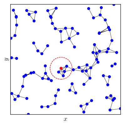
Figure 1: Snapshot of a system of $M=100$ agents and density $\rho=0.0512$. Agents within a distance $d=\alpha d_{0}$, where $d_{0}=1/\sqrt{\rho}$ and $\alpha=1$, are connected by a link. The dashed circle of radius $d$ centered at the target agent determines its influence neighborhood, which comprises four agents in this example. Links that cross the square box borders are not shown for sake of clarity.

Each agent is represented by a binary string of length $N$, whose bits are initially drawn at random with equal probability for $0$ and $1$. The agents explore the NK-fitness landscape aiming at finding its global maximum by flipping bits following the rules of the imitative learning search Fontanari_15 , which consist basically of copying a bit of the fittest agent in their influence neighborhoods as will be described in detail in this section. In addition, the agents move randomly around the square box, thus changing their influence neighborhoods and, in principle, affecting the efficiency of the imitative search. Next we describe the movement in the $2^{N}$-dimensional space of the binary strings and the physical motion on the square box. Henceforth we will use the terms agent and string interchangeably.

The dynamics begins with the selection of an agent at random, the so-called target agent, at time $t=0$ and comprises two stages. The first stage is the motion on the square box: an angle $\theta\in\left[0,2\pi\right)$ is chosen randomly to give the direction of motion and then a fixed step of length $\delta d_{0}$ with $\delta\geq 0$ is taken on that direction. Once the target agent is at the new position, a circle of radius $d=\alpha d_{0}$ is drawn around it so that its influence neighborhood is determined, as shown in Fig. 1. Then the second stage, namely, the update of the string of the target agent (or the target string, for simplicity) sets in. If the influence neighborhood is empty, i.e. there is no agent within a distance $d$ from the target agent, or all agents in the influence neighborhood have fitness lower than or equal to the fitness of the target agent, then the target agent simply flips a bit at random. Note that due to the nature of the NK-fitness landscape, two agents that have the same fitness must be identical (clones).

A more interesting situation is when there are agents with fitness higher than the fitness of the target agent in its influence neighborhood. Then there are two possibilities of action. The first, which happens with probability $1-p$, consists of flipping a bit at random of the target string as before. The second, which happens with probability $p$, is the imitation of a model string, which is the string of highest fitness in the influence neighborhood of the target agent. In this case, the model and the target strings are compared and the different bits are singled out. Then the target agent selects at random one of the distinct bits and flips it so that this bit is now the same in both strings. Hence, imitation results in the increase of the similarity between the target and the model agents, which may not necessarily lead to an increase of the fitness of the target agent if the landscape is not additive, i.e. for $K>0$.

The parameter $p\in\left[0,1\right]$ is the imitation probability, which we assume is the same for all agents (see Fontanari_16 for the relaxation of this assumption). The case $p=0$ corresponds to the baseline situation in which the agents explore the state space independently of each other and so, in this case, the motion on the square box has no effect at all on the performance of the search. The case $p=1$ corresponds to the situation where only the model strings explore the state space through random bit flips, whereas the other strings simply follow the models in their influence neighborhoods. The imitation procedure described above was borrowed from the incremental assimilation mechanism Shibanai_01 ; Avella_10 ; Peres_11 used to study the influence of external agencies in the celebrated Axelrod’s model of social influence Axelrod_97 .

After the target agent is updated, which means performing a step of size $\delta d_{0}$ in a random direction and flipping a bit of its string, we increment the time $t$ by the quantity $\Delta t=1/M$. Then another agent is selected at random and the procedure described above is repeated. Note that during the increment from $t$ to $t+1$, exactly $M$ moves and string operations are performed, though not necessarily by $M$ distinct agents. This asynchronous update seems more appropriate to simulate the continuous-time motion of the agents, as well as the bit changes in the strings. Use of an alternative synchronous update would introduce a global clock that has no counterpart in the problem we seek to model.

The search ends when one of the agents finds the global maximum and we denote by $t^{*}$ the halting time. The efficiency of the search is measured by the total number of string operations necessary to find that maximum, i.e. $Mt^{*}$, and so the computational cost of the search is defined as

$$C=Mt^{*}/2^{N},$$ (2)

where, for convenience, we have rescaled $t^{*}$ by the size of the state space $2^{N}$. To aid the understanding of the model, in the Appendix we offer a probabilistic description of the states of the agents and derive a master equation for the imitative search.

IV Results

To evaluate the performance of the imitative search we use, as usual, the mean computational cost $\langle C\rangle$, which is obtained by averaging the computational cost $C$ over $10^{5}$ searches for the same landscape realization. Since our main concern here is the spatial distribution and motion of the agents on the square box, we will fix the imitation probability to $p=0.5$, and focus on the system size $M$ as well as on the parameters $\alpha$ and $\delta$ that specify the radius of the influence neighborhood and the step size of the random motion of the agents, respectively.

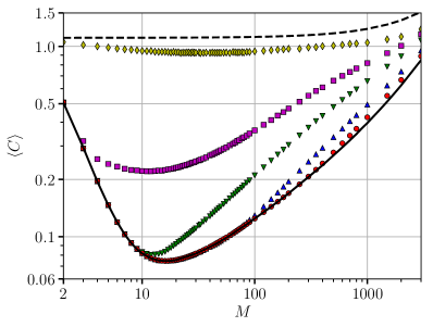
Figure 2: Mean computational cost $\langle C\rangle$ as function of the system size $M$ for the position-fixed scenario ($\delta=0$). The imitation probability is $p=0.5$ and the radius of the influence neighborhood is $d=\alpha d_{0}$ with $\alpha=0.25(\blacklozenge),1(\blacksquare),2(\blacktriangledown),5(\blacktriangle)$ and $10(\CIRCLE)$. The solid curve is the result for the fully connected system and the dashed curve is the analytical result for the independent search Fontanari_15 . The upper panel shows the results for the smooth landscape ($K=0$) and the lower panel for the rugged landscape ($K=4$).

IV.1 Position-fixed scenario

To better appreciate the influence of the mobility on the performance of the imitative search, we study first the case where the agents remain fixed at their (random) positions specified in the initial set up of the system. This position-fixed scenario (i.e. $\delta=0$) is useful for understanding the role of the parameter $\alpha$ that determines the radius of the influence neighborhood, $d=\alpha d_{0}$, where $d_{0}$ is the linear size of the agent.

Figure 2 shows that the effect of $\alpha$ on the mean computational cost depends on the ruggedness of the landscape. As expected, when $\alpha<1$, so that the interaction distance is less than the size of the agent $d_{0}$, the agents explore the state space practically independent of each other and the computational cost is essentially the same as the cost of the independent search, which is very little sensitive to changes on $M$, provided that $M\ll 2^{N}$ (see Fontanari_15 for the analytical derivation of the computational cost of the independent search). The parameter $\alpha$ correlates strongly with the average connectivity $\langle k\rangle$ of the influence network, which is solely determined by the influence neighborhoods of the agents and by the system size $M$, as shown in Fig. 3. This correlation explains the effect of $\alpha$ on the performance of the search. In fact, since for the smooth landscape ($K=0$) the fitness of the agents offer reliable information about their distances to the global maximum, expanding the influence neighborhoods while keeping $M$ fixed increases the odds of finding a high fitness model agent, which then boosts the system performance. In this case, the best performance is achieved by a fully connected system, which is shown in Fig. 2 as a solid curve for clarity purposes, although the results were also obtained through simulations.

The scenario changes drastically for the rugged landscape ($K=4$) due to the presence of local maxima whose main detrimental effect is to uncouple the fitness of an agent from its distance to the global maximum. As a result, agents at local maxima spread unreliable information to their followers that may trap the entire system in a suboptimal solution. The catastrophic performance observed in the case of densely connected networks and large system sizes is akin to the Groupthink phenomenon Janis_82 , when everyone in a group starts thinking alike, which can occur when people put unlimited faith in a leader (the model agent). A way of circumventing Groupthink is to limit or delay the flow of information among the agents and this can be achieved by reducing their influence neighborhood or, equivalently, the average connectivity of the influence network Rodrigues_16 (see Fig. 3). There is, however, a tradeoff between avoiding the local maximum traps and optimizing the search performance. For instance, the choice $\alpha=1$ (see lower panel of Fig. 2) avoids those traps altogether and always yields a superior performance compared with the independent search, but it misses the optimal performance that can be achieved for larger values of $\alpha$ at $M\approx 12$. These large values of $\alpha$, however, expand the influence neighborhoods thus making the system much more susceptible to Groupthink as shown in Fig. 2.

Large systems increase the attractivity of the local maxima, thus producing the undesired Groupthink, because they allow the existence of several copies of the model agent in a same influence neighborhood. Although the model agent can escape the local maximum by flipping a bit at random according to the rules of the imitative search, the extra copies will quickly attract the updated model agent back to the local maximum, resulting in the very high computational costs shown in Fig. 2 for the rugged landscape. For the smooth landscape, however, a large system size results in an increased computational cost (though it is always smaller than the cost of the independent search) simply because of duplication of work since only $M\approx N=12$ agents are necessary to explore the neighborhood of the model string and thus to find a fitter string that is closer to the global maximum.

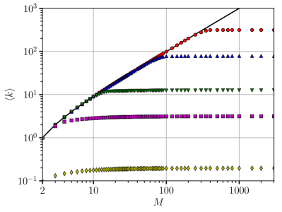
Figure 3: Average connectivity $\langle k\rangle$ of the influence network as function of the system size $M$ for the position-fixed scenario ($\delta=0$). The radius of the influence neighborhood is $d=\alpha d_{0}$ with $\alpha=0.25(\blacklozenge),1(\blacksquare),2(\blacktriangledown),5(\blacktriangle)$ and $10(\CIRCLE)$. The solid curve is the result for the fully connected network, $\langle k\rangle=M-1$. For $M\to\infty$ we have $\langle k\rangle\to\pi\alpha^{2}$.

For small system sizes $M$ and $\alpha$ not too small, the results of Fig. 3 (and of Fig. 2 as well) show that the system is fully connected, i.e., $\langle k\rangle=M-1$. This happens because the density $\rho$ (and hence $d_{0}$) is kept constant so that when $M$ changes, the linear size $L$ of the square box changes too, while the radius of the interaction neighborhood $d=\alpha d_{0}$ remains the same. As a result, for small $M$ (and small $L$) the interaction neighborhood of an agent is likely to comprise the entire square box. In the other extreme, $M\to\infty$ (and hence $L\to\infty$) the agents are uniformly distributed over the square box and so the average number of agents inside the interaction neighborhood of area $\pi d^{2}$ is simply $M\pi d^{2}/L^{2}=\pi\alpha^{2}$, in agreement with the results of Fig. 3.

IV.2 Mobile-agents scenario

We turn now to the more interesting situation where the agents move in random directions with a step of fixed length $\delta d_{0}$. The obvious effect of this motion is to make the influence neighborhood of the agents volatile, but the manner this volatility influences the performance of the imitative search is far from obvious as we will see next.

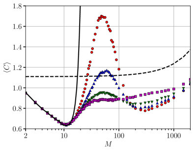
Figure 4: Mean computational cost $\langle C\rangle$ as function of the system size $M$ for mobile agents with step sizes $\delta=0(\CIRCLE),0.5(\blacktriangle),1(\blacktriangledown)$ and $100(\blacksquare)$. The imitation probability is $p=0.5$ and the radius of the influence neighborhood is $d=\alpha d_{0}$ with $\alpha=2$. The solid curve is the result for the fully connected system and the dashed curve is the analytical result for the independent search Fontanari_15 . The upper panel shows the results for the smooth landscape ($K=0$) and the lower panel for the rugged landscape ($K=4$).

Figure 4 shows the influence of the mobility on the computational cost for our two fitness landscapes. A nonzero step size $\delta$ produces only a mild degradation on the performance of the search for the smooth landscape ($K=0$) and so the effect of the mobility in this case is hardly noticeable. For the rugged landscape ($K=4$), however, the mobility is very effective in avoiding the traps of the local maxima without the incurred tradeoff observed in the position-fixed scenario. This is so because the mobility does not change the average connectivity of the influence network. In fact, measurement of the mean degree of the agents by averaging over all the configurations in a run and then averaging over distinct runs yields the same results obtained for the position-fixed scenario (see Fig. 3). Hence, the random motion of the agents does not alter the nature of the influence network. This observation makes the results of Fig.  4 even more remarkable since it reveals that the change in the computational cost is a genuine effect of the mobility of the agents and not a consequence of changing the connectivity of the influence network. Of course, if the system is fully connected, then the mobility will not affect the performance of the search.

Figure 5 reveals the intricate interplay between the parameter $\delta$, which specifies the length of the step $\delta d_{0}$, and the parameter $\alpha$, which determines the radius of the influence neighborhood $\alpha d_{0}$. For large $\alpha$, the computational cost is little affected by the mobility of the agents since the odds that an agent becomes isolated and thus escapes the influence of the local maxima is negligible in this case. For small $\alpha$ the mobility is irrelevant too, as the agents remain isolated regardless of their wanderings on the square box. There is, however, a range of values of $\alpha$ where the mobility is very influential and produces antagonistic effects on the computational cost. For instance, comparison with the lower panel of Fig. 2 indicates that the mobility increases the cost and hence is detrimental for $\alpha=1$, whereas it decreases the cost and hence is beneficial for $\alpha=2$.

The effect of mobility is more noticeable in Fig. 6 where we fix the system size to $M=53$, which corresponds to the maximum of the computational cost in the lower panel of Fig. 4, and vary the step size $\delta$ over several orders of magnitude. Since for this system size the trapping effects of the local maxima are maximized, moving the model agents far away from their clones is an efficient way to mitigate the influence of those maxima, as seen in the case $\alpha=2$. When the influence of the local maxima is already reduced due to the small influence neighborhoods of the agents, as in the case of $\alpha=1.5$, the mobility can actually help their dissemination over the square box, resulting in the increase of the computational cost. In any event, a large step size $\delta$ guarantees that the imitative search always outperforms the independent search.

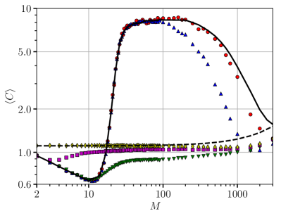
Figure 5: Mean computational cost $\langle C\rangle$ as function of the system size $M$ for mobile agents with step size $\delta=5$. The imitation probability is $p=0.5$ and the radius of the influence neighborhood is $d=\alpha d_{0}$ with $\alpha=0.25(\blacklozenge),1(\blacksquare),2(\blacktriangledown),5(\blacktriangle)$ and $10(\CIRCLE)$. The solid curve is the result for the fully connected system and the dashed curve is the analytical result for the independent search Fontanari_15 . The parameters of the rugged landscape are $N=12$ and $K=4$.

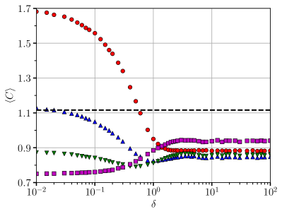
Figure 6: Mean computational cost $\langle C\rangle$ as function of the step size $\delta$ for a system of size $M=53$. The imitation probability is $p=0.5$ and the radius of the influence neighborhood is $d=\alpha d_{0}$ with $\alpha=1.5(\blacksquare),1.8(\blacktriangledown),1.9(\blacktriangle)$ and $2(\CIRCLE)$. The horizontal dashed line is the result for the independent search $\langle C\rangle\approx 1.12$. The parameters of the rugged landscape are $N=12$ and $K=4$.

To verify the soundness of our claim that the high computational cost is caused by the loss of diversity of the system when the search is trapped in the local maxima, we consider the time-dependence of the mean pairwise distance between the $M$ strings in the system

$$\bar{H}=\frac{2}{M\left(M-1\right)}\sum_{k=1}^{M-1}\sum_{l=k+1}^{M}h\left(\mathbf{x}^{k},\mathbf{x}^{l}\right),$$ (3)

where

$$h\left(\mathbf{x}^{k},\mathbf{x}^{l}\right)=\frac{1}{2}-\frac{1}{2N}\sum_{i=1}^{N}(1-2x_{i}^{k})(1-2x_{i}^{l})$$ (4)

is the normalized Hamming distance between the bit strings $\mathbf{x}^{k}$ and $\mathbf{x}^{l}$ Hamming_50 . The quantity $\bar{H}$ can be interpreted as follows: if we pick two strings at random, they will differ by $N\bar{H}$ bits on average, and so $\bar{H}$ measures the diversity of the strings in the system. Figure 7 shows the effect of the step size $\delta$ on the time evolution of $\bar{H}$ for single runs of the imitative search. The panels show the results for two values of the radius of influence of the agents $\alpha d_{0}$, viz., $\alpha=2$ and $\alpha=4$. Since the initial strings are chosen randomly, one has $\bar{H}=0.5$ at $t=0$, which corresponds to the maximum diversity. For $\alpha=2$, highly mobile agents can maintain the high diversity of the system during the entire search, thus indicating that the local maxima have little influence on the computational cost in accord with Fig. 4. In the case of motionless agents ($\delta=0$), however, the diversity decreases somewhat abruptly in the first half of the search, resulting in a situation where the strings differ from each other by $2.5$ to $3.5$ bits on average, which hints that the search is stuck in local maxima. In the second half of the search, the diversity increases slowly, suggesting that a fraction of the agents managed to escape the local maximum traps and found their way to the global maximum. For $\alpha=4$, the trapping effects of the local maxima are greatly enhanced, as expected. Although highly mobile agents can delay the fall into those traps, the search eventually gets stuck resulting in the confinement of a substantial fraction of the agents in the neighborhoods of the local maxima. These results thus support our claim that the loss of diversity (i.e. Groupthink) due to the trapping effects of the local maxima is the ultimate culprit for the high computational cost of the imitative search.

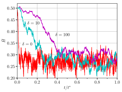
Figure 7: Time evolution of the mean pairwise Hamming distance $\bar{H}$ for single runs of a system of size $M=53$ and step sizes $\delta=0$, $\delta=10$ and $\delta=100$ as indicated. The time $t$ is scaled by the halting time $t^{*}$ of each search. The imitation probability is $p=0.5$ and the radius of the influence neighborhood is $d=\alpha d_{0}$ with $\alpha=2$ (upper panel) and $\alpha=4$ (lower panel). The parameters of the rugged landscape are $N=12$ and $K=4$.

In our model, the exploration of the state space of the NK-fitness landscape halts at $t^{*}$ when one of the agents reaches the global maximum. If, however, the search is allowed to continue, then the agent that first found the global maximum will quickly attract the rest of the group to its neighborhood, similarly to what happens for the local maxima. The strength of the attraction decreases with increasing mobility as shown in the lower panel of Fig. 7. Hence a considerable number of agents will be at or in the close vicinity of the global maximum after $t^{*}$, so a more stringent halting criterion will not significantly affect the computational cost.

A word is in order about an intriguing feature of the imitative search manifested in Figs. 2 and 4 for the rugged landscape ($K=4$), namely, the appearance of a shallower minimum of the computational cost for $M\approx 300$ and not too large step sizes. The explanation has to do with the antagonistic effects of varying the system size. On the one hand, increasing $M$ beyond the optimal size ($M\approx 12$) allows the appearance of clones of the model string, which strengthens the attractivity of the local maxima and leads to the sharp increase of the computational cost shown in those figures. On the other hand, increasing $M$ makes the network sparser and delays the flow of information over it, which reduces the influence of the local maxima. To see this we calculate the average path length $\bar{l}$ of the influence networks, defined as the average number of steps along the shortest paths for all possible pairs of network nodes Newman_10 . This calculation is done for systems with $\alpha\geq 2$ only, for which the shallower minimum appears (see Fig. 2) and whose influence networks have a high average connectivity $\langle k\rangle>12$ (see Fig. 3) so we can guarantee that they are connected. For the (connected) influence networks with fixed $d=\alpha d_{0}$ we find that $\bar{l}$ increases with $M^{0.47}$ as in the regular square lattice Vragovic_05 (it increases with $\ln M$ for Erdős-Rényi graphs Albert_02 ), which justifies our claim that information flows slower for large $M$. It is this weakening of the influence of the local maxima that leads to the shallower minimum of the computational cost exhibited in Figs. 2 and 4. Lastly, further increase of $M$ leads to performance degradation due to the duplication of work as in the case of the smooth landscape.

The antagonistic effects of increasing the system size on the dynamics of the search (creation of clones boosts the attractivity of the local maxima) and on the topology of the influence network (slow down of the flow of information in the system) are behind the nontrivial outcomes discussed in this section. In addition, the position-fixed scenario ($\delta=0$) yields the best performance for the second-best system size because for sparse networks (see, e.g., the results for $\alpha=1.5$ in Fig. 6) the mobility speeds up the dissemination of the local maxima over the square box.

Finally, we mention that we also considered different realizations of rugged landscapes with $K=4$, as well as landscapes with distinct degrees of epistasis, and found that the same qualitative conclusions regarding the roles of the parameters $\alpha$ and $\delta$ hold true for every landscape realization.

V Discussion

It has long been known that patterns of communication, i.e. who can communicate with whom, have a strong influence on the problem-solving efficiency of groups Bavelas_50 ; Leavitt_51 (see Mason_12 ; Sebastian_17 for more recent contributions). These studies focused on imposed or fixed communication patterns, which is typical of the military and industrial organizations, thus excluding a priori the possibility of self-organization of the group members. A simple way to introduce flexibility on the patterns of communication is to allow the agents to roam around an arena where they can interact with each other if the distance between them is less than a prespecified threshold. Within this roaming scenario, we study the performance of cooperative problem-solving systems that use imitative learning Fontanari_14 as the search strategy to find the global maxima of NK-fitness landscapes.

We find that for smooth landscapes, i.e. landscapes with a single maximum, mobility is always slightly detrimental to the imitative search performance. Hence in the case the information exchanged among the agents (i.e., their fitness values) correlates strongly with their distances to the global maximum, the best strategy is to maintain and strengthen the local spatial correlations between the agents by keeping them fixed at their initial positions. However, for rugged landscapes, where the presence of local maxima uncouples the fitness values from the distances to the global maximum, imitation of high fitness agents may lead to entrapment in the local maxima. In this case, mobility offers a mechanism to circumvent those traps with the guarantee of always outperforming the independent search and reproducing the overall optimal performance achieved by fully-connected small systems.

We stress that our study of the imitative search does not seek to offer an alternative heuristic to tackle optimization problems. Rather, it seeks to assess quantitatively the potential of imitative learning as the underlying cooperative mechanism of task-oriented groups. In fact, since finding the global maxima of NK landscapes with $K>0$ is an NP-Complete problem Solow_00 , we do not expect that the imitative search (or, for that matter, any other search strategy) will reach those maxima much more rapidly than the independent search. However, finding the solution much more slowly than the independent search, as observed for certain values of the group size $M$ (see, e.g., Fig. 5), is a bad omen for a search strategy. But this negative outcome is actually the main thrust of the imitative search since it is akin to a well-known maladaptive behavior associated to social learning, namely, the Groupthink phenomenon that occurs when everyone in a group starts thinking alike Janis_82 .

Nevertheless, it is instructive to compare the imitative search with the evolutionary algorithms Back_96 as there are clear similarities between those two heuristics. In particular, flipping a randomly chosen bit of the target string resembles the mutation operator of the evolutionary algorithms, except that in those algorithms mutation is an error of the reproduction process, whereas in the imitative search flipping a bit at random and imitating the model string are mutually exclusive processes. In addition, imitation resembles the crossover process of genetic algorithms, with the caveat that the model agent is a mandatory parent in all mates but it contributes only a single bit to the offspring, which then replaces the other parent, namely, the target agent. More importantly, the bit passed to the offspring is not random since it must be absent in the target string. This aspect highlights the fact that the imitative search models cultural, rather than genetic, inheritance.

An appealing feature of the imitative search strategy as a model of human cooperation in problem solving is the emergence of Groupthink. Real-life remedies for this issue include the call for outside experts to share their viewpoints with the group members and the leave of members to facilitate exposure to fresh ideas outside the influence of the group. Both ventures involve the notion of mobility, hence our interest in finding out whether mobility has similar beneficial effects on the imitative learning search too. However, the way we introduce mobility in the search, such that all members of the group can move thus allowing a group to break apart due to the motion of its members, does not tally with the aforementioned remedies. A metapopulation approach where the group is composed of stable subgroups and the agents can migrate between them seems to offer a more suitable scenario to describe those situations. Nevertheless, our scenario offers a first step in the study of the effects of the flexibility on the patterns of communication and our finding that the random motion of agents can avoid Groupthink supports the common sense view that some kind of mobility is beneficial to group problem solving.

Appendix A

In this appendix we sketch a probabilistic description of the states of the agents evolving under the rules of the imitative search described in Section III. We begin by introducing some notation. The state of agent $k$ is represented by the binary string $\mathbf{x}^{k}=\left(x_{1}^{k},\ldots,x_{N}^{k}\right)$ with $x_{i}^{k}=0,1$; $i=1,\ldots,N$ and $k=1,\ldots,M$. The set of agents, including agent $k$, in the influence neighborhood of agent $k$ is denoted by $\Omega_{k}$. At time $t$, the model agent $m$ in $\Omega_{k}$ is represented by the string $\mathbf{x}^{m}$ so that $\mathcal{F}\left(\mathbf{x}^{m}\right)\geq\mathcal{F}\left(\mathbf{x}^{l}\right)$ for all $l\in\Omega_{k}$. In addition, we let $\mathbf{\tilde{x}}^{k_{i}}=\left(x_{1}^{k},\ldots,x_{i-1}^{k},1-x_{i}^{k},x_{i+1}^{k},\ldots,x_{N}^{k}\right)$ represent the state of agent $k$ that differs from $\mathbf{x}^{k}$ solely at bit $i$.

Since in the elemental time interval $\Delta t=1/M$ application of the update rules results always in the flipping of one bit of the target agent, the state of agent $k$ will only change when it is chosen as the target agent, which happens with probability $1/M$. The probability $P_{t+\Delta t}\left(\mathbf{x}^{k}\right)$ that agent $k$ is represented by the string $\mathbf{x}^{k}$ at time $t+\Delta t$ is then written as

$$P_{t+\Delta t}\left(\mathbf{x}^{k}\right) = \frac{1}{M}\left(1-p\right)\frac{1}{N}\sum_{i}^{N}P_{t}\left(\mathbf{\tilde{x}}^{k_{i}}\right)$$ (5)

$$\mbox{}+\frac{1}{M}p\frac{1}{N}\sum_{i}^{N}P_{t}\left(\mathbf{\tilde{x}}^{k_{i}}\right)\delta\left(\mathbf{\tilde{x}}^{k_{i}},\mathbf{x}^{m}\right)$$

$$\mbox{}+\frac{1}{M}p\frac{1}{N}\sum_{i}^{N}P_{t}\left(\mathbf{\tilde{x}}^{k_{i}}\right)\Lambda\left(\mathbf{x}^{k},\mathbf{\tilde{x}}^{k_{i}},\mathbf{x}^{m}\right)$$

$$\mbox{}+\left(1-\frac{1}{M}\right)P_{t}\left(\mathbf{x}^{k}\right)$$

where

$$\Lambda\left(\mathbf{x}^{k},\mathbf{\tilde{x}}^{k_{i}},\mathbf{x}^{m}\right)=\frac{\left[1-\delta\left(\mathbf{\tilde{x}}^{k_{i}},\mathbf{x}^{m}\right)\right]\delta\left(x_{i}^{k},x^{m}_{i}\right)}{\sum_{j}^{N}\left[1-\delta\left(\tilde{x}_{j}^{k_{i}},x^{m}_{j}\right)\right]},$$ (6)

with $\delta\left(\mathbf{x},\mathbf{y}\right)=1$ if the binary strings $\mathbf{x}$ and $\mathbf{y}$ are identical and $\delta\left(\mathbf{x},\mathbf{y}\right)=0$, otherwise. We have also used the scalar version of this function, namely, the Kronecker delta, $\delta\left(x,y\right)=1$ if $x=y$ and $0$, otherwise.

The first term on the LHS of eq. (5) describes the random flipping of a bit, which occurs with probability $1-p$, and accounts for the possibility that at time $t$ the state of agent $k$ is $\mathbf{\tilde{x}}^{k_{i}}$ and that bit $i$ is flipped. The second term on the LHS of eq. (5) describes the imitation procedure, which happens with probability $p$, for the special situation where agent $k$, whose state is $\mathbf{\tilde{x}}^{k_{i}}$, is the model agent at time $t$. We recall that in this case, the target agent flips a bit at random. The third term on the LHS of eq. (5) describes the general imitation process when the target string differs from the model string. As before, the state of agent $k$ at time $t$ is $\mathbf{\tilde{x}}^{k_{i}}$, but now bit $i$ must be copied from the model string. The probability of this event is given by the reciprocal of the number of different bits in strings $\mathbf{\tilde{x}}^{k_{i}}$ and $\mathbf{x}^{m}$, i.e., the reciprocal of the Hamming distance between these two strings. We note that $\mathbf{\tilde{x}}^{k_{i}}$ and $\mathbf{x}^{m}$ differ by one bit at least, namely, bit $i$, so the denominator in eq. (6) never vanishes. Finally, the fourth term on the LHS of eq. (5) accounts for the case that the state of agent $k$ at time $t$ is $\mathbf{x}^{k}$ and that this agent is not chosen as the target agent.

Using $\Delta t=1/M$ we can rewrite eq. (5) as

$$\frac{\Delta P_{t}\left(\mathbf{x}^{k}\right)}{\Delta t} = -P_{t}\left(\mathbf{x}^{k}\right)+\frac{1-p}{N}\sum_{i}^{N}P_{t}\left(\mathbf{\tilde{x}}^{k_{i}}\right)$$ (7)

$$\mbox{}+\frac{p}{N}\sum_{i}^{N}P_{t}\left(\mathbf{\tilde{x}}^{k_{i}}\right)\delta\left(\mathbf{\tilde{x}}^{k_{i}},\mathbf{x}^{m}\right)$$

$$\mbox{}+\frac{p}{N}\sum_{i}^{N}P_{t}\left(\mathbf{\tilde{x}}^{k_{i}}\right)\Lambda\left(\mathbf{x}^{k},\mathbf{\tilde{x}}^{k_{i}},\mathbf{x}^{m}\right)$$

where $\Delta P_{t}\left(\mathbf{x}^{k}\right)=P_{t+\Delta t}\left(\mathbf{x}^{k}\right)-P_{t}\left(\mathbf{x}^{k}\right)$. Hence the continuous-time limit is obtained for $M\to\infty$. To take into account the fact that the search stops at the global maximum $\mathbf{x}^{g}$, we need only to add the proviso that $\mathbf{x}^{g}$ does not appear in the argument of $P_{t}$ on the LHS of eq. (7), i.e., $\mathbf{x}^{g}$ is a perfect trap. In addition to the high dimensionality of the state variables, the difficulty to iterate eq. (7) is due to the determination of the model string $\mathbf{x}^{m}$, which is actually the term that couples the $M$ agents in the system. In particular, $\mathbf{x}^{m}$ is the string that maximizes $\mathcal{F}\left(\mathbf{x}^{l}\right)$ for $l\in\Omega_{k}$ with the constraints that $P_{t}\left(\mathbf{x}^{m}\right)>0$ and $\mathbf{x}^{m}\neq\mathbf{x}^{g}$, since the global maximum is never a model string in the imitative search. Finally, we note that in the case of mobile agents we need to include a time dependence on the influence neighborhoods $\Omega_{k}$ and specify how they change with time.

References

- (1) R. Boyd and P.J. Richerson, The Origin and Evolution of Cultures (Oxford University Press, Oxford, 2005).
- (2) L. Rendell, R. Boyd, D. Cownden, M. Enquist, K. Eriksson, M.W. Feldman, L. Fogarty, S. Ghirlanda, T. Lillicrap, and K.N. Laland, Science 328, 208 (2010).
- (3) M. Perc, J.J. Jordan, D.G. Rand, Z. Wang, S. Boccaletti, and A. Szolnoki, Phys. Rep. 687, 1 (2017).
- (4) H. Bloom, Global Brain: The Evolution of Mass Mind from the Big Bang to the 21st Century (Wiley, New York, 2001).
- (5) S. Blackmore, The Meme Machine (Oxford University Press, Oxford, 2000).
- (6) J.F. Fontanari, PLoS ONE 9, e110517 (2014).
- (7) J.F. Fontanari, Eur. Phys. J. B 88, 251 (2015).
- (8) I.L. Janis, Groupthink: psychological studies of policy decisions and fiascoes (Houghton Mifflin, Boston, 1982).
- (9) S.A. Kauffman and S. Levin, J. Theor. Biol. 128, 11 (1987).
- (10) K. Zhao, J. Stehlé, G. Bianconi, and A. Barrat, Phys. Rev. E 83, 056109 (2011).
- (11) http://www.sociopatterns.org.
- (12) C. Cattuto, W. Van den Broeck, A. Barrat, V. Colizza, J.-F. Pinton, and A. Vespignani, PLoS ONE 5, e11596 (2010).
- (13) M. Starnini, A. Baronchelli, A. Barrat, and R. Pastor-Satorras, Phys. Rev. E 85, 056115 (2012).
- (14) M. Starnini, A. Baronchelli, and R. Pastor-Satorras, Phys. Rev. Lett. 110, 168701 (2013).
- (15) A. Sapienza, A. Barrat, C. Cattuto, and L. Gauvin, Phys. Rev. E 98, 012317 (2018).
- (16) A. Moinet, R. Pastor-Satorras, and A. Barrat, Phys. Rev. E 97, 012313 (2018).
- (17) N. Perra, B. Gonçalves, R. Pastor-Satorras, and A. Vespignani, Sci. Rep. 2, 469 (2012).
- (18) M. Frasca, A. Buscarino, A. Rizzo, L. Fortuna, and S. Boccaletti, Phys. Rev. Lett. 100, 044102 (2008).
- (19) N. Fujiwara, J. Kurths, and A. Díaz-Guilera, Phys. Rev. E 83, 025101(R) (2011).
- (20) S. Meloni, A. Buscarino, L. Fortuna, M. Frasca, J. Gómez-Gardeñes, V. Latora, and Y. Moreno, Phys. Rev. E 79, 067101 (2009).
- (21) A. Cardillo, S. Meloni, J. Gómez-Gardeñes, and Y. Moreno, Phys. Rev. E 85, 067101 (2012).
- (22) V. Colizza, A. Barrat, M. Barthelemy, and A. Vespignani, Proc. Natl. Acad. Sci. 103, 2015 (2006).
- (23) A. Buscarino, L. Fortuna, M. Frasca, and V. Latora, EPL 82, 38002 (2008).
- (24) S.A. Kauffman, At Home in the Universe: The Search for Laws of Self-Organization and Complexity (Oxford University Press, New York, 1995).
- (25) D.A. Levinthal, Manag. Sci. 43, 934 (1997).
- (26) D. Lazer and A. Friedman, Admin. Sci. Quart. 52, 667 (2007).
- (27) S. Billinger, N. Stieglitz, and T.R. Schumacher, Organ. Sci. 25, 93 (2013).
- (28) B. Derrida, Phys. Rev. B 24, 2613 (1981).
- (29) D. Solow, A. Burnetas, M. Tsai, and N.S. Greenspan, Complex Systems 12, 423 (2000).
- (30) E. Gilbert, J. Soc. Indust. Appl. Math. 9, 533 (1961).
- (31) J.F. Fontanari, EPL 113, 28009 (2016).
- (32) Y. Shibanai, S. Yasuno, and I. Ishiguro, J. Conflict. Res. 45, 80 (2001).
- (33) J. González-Avella, M. Cosenza, V.M Eguíluz, and M. San Miguel, New J. Phys. 12, 013010 (2010).
- (34) L.R. Peres and J.F. Fontanari, EPL 96, 38004 (2011).
- (35) R. Axelrod, J. Conflict Res. 41 203 (1997).
- (36) J.F. Fontanari and F.A. Rodrigues, Theory Biosci. 135, 101 (2016).
- (37) R.W. Hamming, Bell Syst. Tech. J. 29, 147 (1950).
- (38) M. Newman, Networks: An Introduction (Oxford University Press, New York, 2010).
- (39) I. Vragović, E. Louis, and A. Díaz-Guilera, Phys. Rev. E 71, 036122 (2005).
- (40) R. Albert and A.-L. Barabási, Rev. Mod. Phys. 74, 47 (2002).
- (41) A. Bavelas, J. Acoustical Soc. Amer. 22 725 (1950).
- (42) H.J. Leavitt, J. Abnorm. Soc. Psych. 46 38 (1951).
- (43) W. Mason and D.J. Watts, Proc. Natl. Acad. Sci. 109 764 (2012).
- (44) S.M. Reia, S. Herrmann, and J.F. Fontanari, Phys. Rev. E 95, 022305 (2017).
- (45) T. Bäck, Evolutionary Algorithms in Theory and Practice: Evolution Strategies, Evolutionary Programming, Genetic Algorithms (Oxford University Press, New York, 1996).