(Sequential) Importance Sampling Bandits

Abstract

This work extends existing multi-armed bandit (MAB) algorithms beyond their original settings by leveraging advances in sequential Monte Carlo (SMC) methods from the approximate inference community. We leverage Monte Carlo estimation and, in particular, the flexibility of (sequential) importance sampling to allow for accurate estimation of the statistics of interest within the MAB problem. The MAB is a sequential allocation task where the goal is to learn a policy that maximizes long term payoff, where only the reward of the executed action is observed; i.e., sequential optimal decisions are made, while simultaneously learning how the world operates. In the stochastic setting, the reward for each action is generated from an unknown distribution. To decide the next optimal action to take, one must compute sufficient statistics of this unknown reward distribution, e.g., upper-confidence bounds (UCB), or expectations in Thompson sampling. Closed-form expressions for these statistics of interest are analytically intractable except for simple cases. By combining SMC methods — which estimate posterior densities and expectations in probabilistic models that are analytically intractable — with Bayesian state-of-the-art MAB algorithms, we extend their applicability to complex models: those for which sampling may be performed even if analytic computation of summary statistics is infeasible — nonlinear reward functions and dynamic bandits. We combine SMC both for Thompson sampling and upper confident bound-based (Bayes-UCB) policies, and study different bandit models: classic Bernoulli and Gaussian distributed cases, as well as dynamic and context dependent linear-Gaussian, logistic and categorical-softmax rewards.

1 Introduction

The multi-armed bandit (MAB) problem considers the strategy one must devise when playing a row of slot machines: i.e., which arms to play to maximize returns. This analogy extends to a wide range of interesting real-world challenges that require online learning while simultaneously maximizing some notion of reward. The arm may be a medicine a doctor must prescribe to a patient, the reward being the outcome of such treatment on the patient; or the set of resources a manager needs to allocate to competing projects, with the reward being the revenue attained at the end of the month; or the ad/product/content an online recommendation algorithm must choose to display to maximize click-through rate in e-commerce. The contextual MAB setting, where at each interaction with the world side information (known as ‘context’) is available, is a natural extension of this abstraction. The ‘context’ is the physiology of the patient, the type of resources available for each project, or the features of the website user.

Interest in sequential decision processes has recently intensified in both academic and industrial communities, with the surge of advanced reinforcement learning techniques within the machine learning community (80) . Reinforcement learning has now been successfully applied in a wide variety of domains, from hyperparameter tuning (44) and Monte Carlo tree search (9) for complex optimization in science and engineering problems, to revenue maximization (35) and marketing solutions (77) in business and operations research. Besides, reinforcement learning is gaining popularity in e-commerce and digital services as well, improving online advertising at LinkedIn (2), engagement with website services in Amazon (41), recommending targeted news at Yahoo (56), and allowing full personalization of content and art at Netflix (65). The techniques used in these online success stories are grounded on statistical advances on sequential decision processes, yet raise interesting challenges that state-of-the art MAB algorithms do not address.

The MAB setting, as it crystallizes the fundamental trade-off between exploration and exploitation in sequential decision making, has been studied throughout the 20th century, with important contributions by Thompson (81) and later Robbins (73). Over the years, several algorithms have been proposed to overcome the exploration-exploitation tradeoff in the MAB problem (53). The $\epsilon$-greedy approach (i.e., to be greedy with probability $1-\epsilon$, and to play the arm with best reward so far, otherwise to randomly pick an arm) has become very popular due to its simplicity, while retaining often good performance (8). Gittins (38) formulated a more sophisticated method, based on computing the optimal strategy for certain bandit scenarios, where geometrically discounted future rewards are considered. Since the exact computation of the Gittins index is complicated in practical settings, approximations have been developed as well (15).

Lai and Robbins (51) introduced a new class of algorithms, based on the upper confidence bound (UCB) of the expected reward of each arm, for which strong theoretical guarantees have been proven (50), and many extensions proposed (37, 36). Bayesian counterparts of UCB-type algorithms (46), where quantiles of posterior distributions are used as proxies for confidence bounds, have been shown to provide an unifying framework for many UCB-based variants for distinctive bandit problems. In par with UCB, Thompson sampling (81, 76) is one of the most celebrated and studied exploration strategies in stochastic MABs, which readily fit into the Bayesian learning framework as well. Bayesian modeling of the MAB problem facilitates not only generative and interpretable modeling, but sequential and batch processing algorithm development as well.

Both UCB and Thompson sampling based strategies have been theoretically studied, and shown to be near optimal in classic (36, 3) and linear (1, 4, 5, 74, 75) bandits. However, these algorithms do not typically generalize easily to complex problems, as maintaining exact posteriors is intractable for distributions not in the exponential family (49, 76). In general, efficient approximations to high-probability confidence sets, as well as posterior distributions, need to be designed. Developing practical MAB methods to balance exploration and exploitation in complex domains remains largely unsolved.

In an effort to extend MAB algorithms to more complex scenarios, researchers have considered other flexible reward functions and Bayesian inference. A first step beyond the classic Bernoulli MAB setting for context-dependent binary rewards was the use of Laplace approximations for Thompson sampling (18), and more recently, the Polya-Gamma augmentation (31). These techniques are specifically targeted to binary rewards, modeled via the logistic function. Recent approaches have embraced Bayesian neural networks and approximate inference to accommodate complex reward functions.

Bootstrap sampling for example has been considered for Thompson sampling in classic bandits (34), as well as for deep network based reinforcement learning (68). Variational methods, stochastic mini-batches, and Monte Carlo techniques have been studied for uncertainty estimation of reward posteriors (13, 48, 58, 69, 54). Riquelme et al. (71) have recently benchmarked some of these techniques, and reported that neural networks with approximate inference, even if successful for supervised learning, under-perform in the MAB setting. In particular, Riquelme et al. (71) emphasize the issue of adapting the slow convergence uncertainty estimates of neural net based methods to MABs. In parallel, others have focused on extending Thompson sampling to complex online problems (39) by leveraging ensemble methods (61) or generalized sampling techniques (55). However, all these assume stationary reward functions.

Interesting work to address switching bandit problems has already been proposed, both for UCB (37) and Thompson sampling (63). However, these are limited to specific bandit models, i.e., those with abrupt and finite number of changes in the mean rewards. Recent efforts, such as (11) and (70), have studied more flexible time-varying models. The former is targeted to Bernoulli rewards, and it applies discounting to the parameters of its prior Beta distribution, which requires careful case-by-case tuning of the discount parameters for successful performance. The latter imposes a reward ‘variation’ constraint on the evolution of the arms, as the variation of the expected rewards over the relevant time horizon is bounded by a variation budget, designed to depend on the number of bandit pulls.

On the contrary, we here propose to relax these constraints, and yet consider very flexible time-varying models. We study dynamic — also known as restless — bandits, where the world might evolve over time, and rewards are sequentially observed for the played arms. To devise flexible MAB algorithms that are performant, interpretable, and ultimately useful in real-life applications, we ground our research on (sequential) importance sampling-based methods, also known as sequential Monte Carlo (SMC).

Our goal is to design efficient and interpretable sequential decision algorithms by leveraging well-established techniques from statistics and probability theory. We focus on importance sampling based Monte Carlo, which is a general technique for estimating properties of a distribution, using only samples generated from a different distribution. SMC methods (7, 30, 27) are used to estimate posterior densities or expectations in problems with probabilistic models that are too complex to treat analytically, and have been successful in many applications of science and engineering (72, 86, 42, 23).

In the approximate inference literature, Monte Carlo based methods complement the variational approach (12), recently proposed for both general reinforcement learning problems (13, 58), and posterior sampling-based algorithms as well (52, 84). Variational inference provides a very general method for approximating generative models, but does not provide optimality guarantees. On the contrary, SMC methods provide tight convergence guarantees under general assumptions (24, 20).

We here consider SMC for dynamic bandits, where the world (i.e., bandit parameters) is time-varying, and rewards are sequentially observed for the played arms. In order to compute sufficient statistics of the rewards of each arm over time, Bayesian MAB algorithms require sequential updates of their parameter posteriors. To that end, we propose to leverage SMC to approximate each per-arm parameter posterior. These methods extend the applicability of Bayesian MAB algorithms by permitting more complex models: those for which sampling may be performed even if analytic computation of summary statistics is infeasible.

The use of SMC for Thompson sampling has been previously considered, for a probit MAB reward model by Cherkassky and Bornn (19), as well as to update the posterior of the latent features in a probabilistic matrix factorization model in (47) — where a Rao-Blackwellized particle filter that exploits the structure of the assumed model is proposed. With more ambitious goals in mind,  Gopalan et al. (39) show that computing posterior distributions which lack an explicit closed-form with sequential Monte Carlo results in bounded Thompson sampling regret in complex online problems, such as bandit subset arm selection and job scheduling problems. We consider these efforts valuable, as they provide empirical evidence that approximate MC inference can be successfully combined with Thompson sampling.

Here, we argue that SMC-based sequentially updated random measures approximating the true per-arm parameter posteriors allows for the computation of any statistic a MAB policy might require in dynamic bandits. The proposed SMC-based MAB framework diverges from state-of-the-art MAB techniques, and provides a flexible framework for solving a rich class of MAB problems: ($i$) it leverages SMC for both posterior sampling and estimation of sufficient statistics for Bayesian MAB algorithms — i.e., Thompson sampling and upper confident bound-based policies; ($ii$) it addresses restless bandits via the general linear dynamical system — with unknown parameters via Rao-Blackwellization; and ($iii$) it targets complex nonlinear reward models — both stateless and context-dependent distributions.

Our work extends existing MAB policy algorithms beyond their original settings by leveraging the advances in SMC methods from the approximate inference community. We study the general linear dynamical system (which allows for application of the Kalman filter when the parameters are known), and provide the solution for the more interesting unknown parameter case (by combining Rao-Blackwellization and SMC methods).

Our contribution is unique to the MAB problem in that we provide an SMC-based MAB method that:

1. approximates the posterior densities of interest via random measures, with high-probability convergence guarantees;

2. requires knowledge of the reward function only up to a proportionality constant, i.e., it accommodates nonlinear rewards; and

3. is applicable to time-varying parameter models, i.e., dynamic or restless bandits.

In summary, we provide a flexible framework for solving a rich class — dynamic and nonlinear — bandits. We formally introduce the MAB problem and (sequential) Monte Carlo methods in Section 2, before providing the description of the proposed SMC-based MAB framework in Section 3. We evaluate its performance for Thompson sampling and Bayes-UCB based policies in Section 4, and conclude with promising research directions suggested by these results in Section 5.

2 Problem Statement

2.1 Multi-armed bandits

We study the problem of maximizing the rewards resulting from sequentially chosen actions $a\in\mathcal{A}$, named arms in the bandit literature. The reward function is stochastic, parameterized by the intrinsic properties of each arm (i.e., parameters $\theta\in\Theta$), and can potentially depend on a context $x$, e.g., $x\in{\mathbb{R}}^{d}$.

At each round $t$, the reward $y_{t}$ is observed only for the chosen arm $a_{t}\in\mathcal{A}$ (one of $|\mathcal{A}|$ possible arms), and is independently and identically drawn from its distribution: $y_{t}\sim p_{a}(Y|x_{t},\theta_{t,a}^{*})$, the conditional reward distribution for arm $a$, where we allow for time-varying context and parameters (note the subscript _t in both). These per-arm reward distributions are parameterized by $\theta\equiv\theta_{1:t}\equiv\{\theta_{t=1},\cdots,\theta_{t}\}$, where $\theta_{t}$ refers to the union of all per-arm parameters at time $t$, i.e., $\theta_{t}\equiv\{\theta_{a=1,t},\cdots,\theta_{a=A,t}\}$. Note that the true reward distribution corresponds to a unique $\theta^{*}\in\Theta$. This same problem formulation includes static bandits — where parameters are constant (i.e., $\theta_{t,a}^{*}=\theta_{a}^{*},\;\forall t$) — and non-contextual bandits — described by fixing the context to a constant value $x_{t}=x,\forall t$.

In the contextual MAB, one must decide at each time $t$, which arm $a_{t}$ to play based on the available context, e.g., $x_{t}\in{\mathbb{R}}^{d_{X}}$. Given the true model, the optimal action is $a_{t}^{*}=\mathop{\mathrm{argmax}}_{a^{\prime}\in\mathcal{A}}\mu_{t,a^{\prime}}(x_{t},\theta^{*})$, where $\mu_{t,a}(x_{t},\theta^{*})=\mathbb{E}\left\{Y|a,x_{t},\theta^{*}\right\}$ is the conditional expectation of each arm $a$, given the context at time $t$, and the true parameters $\theta^{*}$.

The challenge in MABs is the lack of knowledge about the reward-generating distribution, i.e., uncertainty about $\theta^{*}$ induces uncertainty about the true optimal action $a_{t}^{*}$. One needs to simultaneously learn the properties of the reward distribution, and sequentially decide which action to take next. MAB policies choose the next arm to play, with the goal of maximizing the expected reward, based upon the history observed so far. Previous history contains the set of contexts, played arms, and observed rewards up to time $t$, denoted as $\mathcal{H}_{1:t}=\left\{x_{1:t},a_{1:t},y_{1:t}\right\}$, with $x_{1:t}\equiv(x_{1},\cdots,x_{t})$, $a_{1:t}\equiv(a_{1},\cdots,a_{t})$ and $y_{1:t}\equiv(y_{1,a_{1}},\cdots,y_{t,a_{t}})$.

We use $\pi(a)$ to denote a multi-armed bandit policy, which is in general stochastic on its choices of $a\in\mathcal{A}$. The goal of a policy is to maximize its cumulative reward, or equivalently, to minimize the cumulative regret — the loss incurred due to not knowing the best arm $a_{t}^{*}$ at each time $t$ — i.e., $R_{T}=\sum_{t=1}^{T}y_{t,a^{*}_{t}}-y_{t,a_{t}}$, where $a_{t}\sim\pi(a)$ denotes the arm picked by the policy. Due to the stochastic nature of the problem, we study the expected cumulative regret at time horizon $T$ (not necessarily known a priori)

$$R_{T}=\mathbb{E}\left\{\sum_{t=1}^{T}y_{t,a^{*}_{t}}-y_{t,a_{t}}\right\}\;,\vspace{-1ex}$$ (1)

where the expectation is taken over the randomness in the outcomes $Y$, the arm selection policy $\pi(\cdot)$, and the uncertainty in the true model $\theta^{*}$.

When the true parameters $\theta^{*}$ of the arms are known, one can readily determine the optimal selection policy $a_{t}^{*}=\mathop{\mathrm{argmax}}_{a^{\prime}\in\mathcal{A}}\mu_{t,a^{\prime}}(x_{t},\theta^{*})$. However, when there is a lack of knowledge about the model, one needs to learn the properties of the environment (i.e., the parameters of the reward distribution) as it interacts with the world (i.e., decides which action to take next). Hence, one must take into account the uncertainty on the unknown (and possibly dynamic) parameters.

In a Bayesian approach to the MAB problem, prior knowledge on the model and parameters is incorporated into the algorithm, and as data from interactions with the environment are collected, a Bayesian algorithm updates the parameter posterior, capturing the full state of knowledge via

$$p(\theta_{t}|\mathcal{H}_{1:t})\propto p_{a_{t}}(y_{t}|x_{t},\theta_{t})p(\theta_{t}|\mathcal{H}_{1:t-1})\;,$$ (2)

where $p_{a_{t}}(y_{t}|x_{t},\theta_{t})$ is the likelihood of the observed reward $y_{t}$ after playing arm $a_{t}$ at time $t$. Computation of this posterior is critical in the MAB setting, for algorithms based on both posterior sampling and confidence intervals.

For the former (e.g., Thompson sampling (76)), one uses $p(\theta_{t}|\mathcal{H}_{1:t})$ to compute the probability of an arm being optimal, i.e., $\pi(a)\sim\mathbb{P}\left(a=a_{t+1}^{*}|x_{t+1},\theta_{t},\mathcal{H}_{1:t}\right)$, where the uncertainty over the parameters must be accounted for. Unknown parameters are modeled as random variables with appropriate priors, and the goal is to marginalize over their posterior probability after observing history $\mathcal{H}_{1:t}$ up to time instant $t$, i.e.,

$$\begin{split}\pi(a|x_{t+1},\mathcal{H}_{1:t})&=\mathbb{P}\left(a=a_{t+1}^{*}|x_{t+1},\mathcal{H}_{1:t}\right)=\int\mathbb{P}\left(a=a_{t+1}^{*}|x_{t+1},\theta_{t},\mathcal{H}_{1:t}\right)p(\theta_{t}|\mathcal{H}_{1:t})\mathrm{d}\theta\\ &=\int\mathds{1}\left[a=\mathop{\mathrm{argmax}}_{a^{\prime}\in\mathcal{A}}\mu_{t+1,a^{\prime}}(x_{t+1},\theta_{t})\right]p(\theta_{t}|\mathcal{H}_{1:t})\mathrm{d}\theta_{t}\;.\end{split}$$ (3)

For the latter (e.g., Bayes-UCB), $p(\theta_{t}|\mathcal{H}_{1:t})$ is critical to determine the distribution of the expected rewards

$$p(\mu_{t,a})=\int p(\mu_{t,a}|x_{t},\theta_{t})p(\theta_{t}|\mathcal{H}_{1:t})\mathrm{d}\theta_{t}\;,$$ (4)

required for computation of the expected reward quantile value of interest $q_{t,a}(\alpha_{t})$, i.e.,

$$\mathrm{Pr}\left[\mu_{t,a}>q_{t,a}(\alpha_{t})\right]=\alpha_{t}\;.$$ (5)

Note that we are considering the case wherein $\alpha_{t}$ depends on time, as in (46).

Analytical expressions for the parameter posteriors $p(\theta_{t}|\mathcal{H}_{1:t})$ are available only for few reward functions (e.g., Bernoulli and linear contextual Gaussian), but not for many other useful cases, such as logistic or categorical rewards. Furthermore, computation of the key summary statistics in Eqns. (3) and (5) can be challenging for many distributions. These issues become even more imperative when dealing with dynamic parameters, i.e., in environments that evolve over time. To overcome these issues, we propose to leverage (sequential) importance sampling.

2.2 Sequential Importance Sampling and Sequential Monte Carlo

Monte Carlo (MC) methods are a family of numerical techniques based on repeated random sampling, which have been shown to be flexible enough for both numerical integration and drawing samples from probability distributions of interest (60).

Importance sampling (IS) is a MC technique for estimating properties of a distribution when obtaining samples from the distribution is difficult. The basic idea of IS is to draw, from an alternative distribution, samples which are subsequently weighted to guarantee estimation accuracy (and often reduced variance). These methods are used both to approximate posterior densities, and to compute expectations in probabilistic models, i.e.,

$$\bar{f}=\int f(\varphi)p(\varphi)\mathrm{d}\varphi\;,$$ (6)

when these are too complex to treat analytically.

In short, IS relies on a proposal distribution $\pi(\cdot)$, from which one draws $M$ samples $\varphi^{(m)}\sim\pi(\varphi),\;m=1,\cdots,M$, and a set of weights

$$\widetilde{w}^{(m)}=\frac{p(\varphi^{(m)})}{\pi(\varphi^{(m)})}\;,\quad\text{with}\quad w^{(m)}=\frac{\widetilde{w}^{(m)}}{\sum_{m=1}^{M}\widetilde{w}^{(m)}}\;.$$ (7)

If the support of $\pi(\cdot)$ includes the support of the distribution of interest $p(\cdot)$, one computes the IS estimator of a test function based on the normalized weights $w^{(m)}$,

$$\bar{f}_{M}=\sum_{m=1}^{M}w^{(m)}f\left(\varphi^{(m)}\right)\;,$$ (8)

with convergence guarantees under weak assumptions (60)

$$\bar{f}_{M}\mathop{\longrightarrow}_{M\rightarrow\infty}^{a.s}\bar{f}\;.$$ (9)

Note that IS can also be interpreted as a sampling method where the true posterior distribution is approximated by a random measure

$$p(\varphi)\approx p_{M}(\varphi)=\sum_{m=1}^{M}w^{(m)}\delta\left(\varphi^{(m)}-\varphi\right)\;,$$ (10)

which leads to estimates that are nothing but the test function integrated with respect to the empirical measure

$$\bar{f}_{M}=\int f(\varphi)p_{M}(\varphi)\mathrm{d}\varphi=\sum_{m=1}^{M}f\left(\varphi^{(m)}\right)w^{(m)}\;.$$ (11)

In many science and engineering problems, data are acquired sequentially in time, and one is interested in learning about the state of the world as observations are collected. In these circumstances, one needs to infer all the unknown quantities in an online fashion. Furthermore, it is likely that the underlying parameters evolve over time. If the dynamics are modeled with known linearity and Gaussianity assumptions, then one can analytically obtain the posterior distributions of interest in closed form: i.e., the celebrated Kalman (43) filter.

On the contrary, practical scenarios often require more lax assumptions: nonlinear functions, uncertainty on parameters, non-Gaussian distributions, etc. For these cases, sequential importance sampling (SIS), also known as sequential Monte Carlo (SMC) (30) or particle filtering (PF) (26), has been shown to be of great flexibility and value(72, 86, 42, 23). These are simulation-based methods that provide a convenient solution to computing online approximations to posterior distributions.

In sequential importance sampling, one considers a proposal distribution that factorizes over time

$$\pi(\varphi_{0:t})=\pi(\varphi_{t}|\varphi_{1:t-1})\pi(\varphi_{1:t-1})=\prod_{\tau=1}^{t}\pi(\varphi_{\tau}|\varphi_{1:\tau-1})\pi(\varphi_{0})\;,$$ (12)

which helps in matching the model dynamics $p(\varphi_{t}|\varphi_{1:t-1})$ to allow for recursive evaluation of the importance weights

$$w_{t}^{(m)}\propto\frac{p(\varphi_{t}|\varphi_{1:t-1})}{\pi(\varphi_{t}|\varphi_{1:t-1})}w_{t-1}^{(m)}\;.$$ (13)

One problem with SIS following the above weight update scheme is that, as time evolves, the distribution of the importance weights becomes more and more skewed, resulting in few (or just one) non-zero weights.

To overcome this degeneracy, an additional selection step, known as resampling (57), is added. In its most basic setting, one replaces the weighted empirical distribution with an equally weighted random measure at every time instant, where the number of offspring for each sample is proportional to its weight. This is known as the Sequential Importance Resampling (SIR) method (40), which we rely on for our proposed framework in Section 3. We acknowledge that any of the numerous methodological improvements within the SMC literature — such as alternative resampling mechanisms (57, 62) or advanced SMC algorithms (64, 6) — are readily applicable to our proposed methods, and likely to have a positive performance impact on the proposed MAB.

3 Proposed SMC-based MAB framework

In this work, we leverage sequential Monte Carlo to compute the posteriors and sufficient statistics of interest for a rich-class of MAB problems: nonstationary bandits — modeled via the general linear dynamical system — with complex — both stateless and context-dependent — reward distributions.

Given any reward function, the stochastic MAB with dynamic parameters is governed by the combination of the in-time transition distribution, and the stochastic reward function,

$$\begin{cases}\theta_{t}^{*}\sim p(\theta_{t}^{*}|\theta_{t-1}^{*})\;,\\ y_{t}\sim p_{a_{t}}(Y|x_{t},\theta_{t}^{*})\;.\end{cases}$$ (14)

In dynamic MAB models, the transition distribution is key to compute the necessary statistics of the unknown parameter posterior $p(\theta_{t}|\mathcal{H}_{1:t})$ in Eqn. (2), which is updated over time via

$$p(\theta_{t}|\mathcal{H}_{1:t})\propto p_{a_{t}}(y_{t}|x_{t},\theta_{t})p(\theta_{t}|\theta_{t-1})p(\theta_{t-1}|\mathcal{H}_{1:t-1})\;.$$ (15)

The challenge in these type of bandits is on computing this posterior according to the underlying time-varying dynamics $p(\theta_{t}|\theta_{t-1})$ and reward function $p_{a_{t}}(Y|x_{t},\theta_{t})$. In general, MABs are modeled with per-arm reward functions, each described with its own idiosyncratic parameters, i.e., $p_{a}(Y|x_{t},\theta_{t}^{*})=p_{a}(Y|x_{t},\theta_{t,a}^{*})$, that evolve independently in time: $p(\theta_{t}^{*}|\theta_{t-1}^{*})=\prod_{a=1}^{A}p(\theta_{t,a}^{*}|\theta_{t-1,a}^{*})$. In this work, we adhere to the same approach, and propose to leverage SMC to approximate the true posterior of each per-arm reward parameters.

We present a flexible SIR-based MAB framework that ($i$) is described in terms of generic likelihood and transition distributions, i.e., $p_{a}(Y|x_{t},\theta_{t,a})$ and $p(\theta_{t,a}|\theta_{t-1,a})$, respectively; and ($ii$) is readily applicable for Bayesian MAB algorithms that compute test functions of per-arm parametric reward distributions, e.g., Thompson sampling and upper confident bound-based policies.

We describe in Algorithm 1 how to combine the sequential Importance Resampling (SIR) method as in (40) with Bayesian algorithms — Thompson sampling and Bayes-UCB policies — in dynamic bandits. The flexibility of SMC allows us to consider any likelihood function, which is computable up to a proportionality constant, as well as any time-varying dynamic that can be described by a transition density from which we can draw samples from.

We first describe in detail the proposed SIR-based framework in Section 3.1, before describing in Section 3.2 the specific transition densities $p(\theta_{t,a}|\theta_{t-1,a})$ for the general linear model dynamics considered here, as well as different reward functions that can be readily accommodated within the proposed framework in Section 3.3.

Algorithm 1 SIR for MAB

0:  $A$, $p(\theta_{a})$, $p(\theta_{t,a}|\theta_{t-1,a})$, $p_{a}(y|x,\theta)$, $M$ (for UCB we also require $\alpha_{t}$)

1:  Draw initial samples from the parameter prior

$$\overline{\theta}_{0,a}\sim p(\theta_{a}),\forall a\in A\;,\quad\text{ and }\quad w_{0,a}^{(m)}=\frac{1}{M}\;.$$

2:  for $t=0,\cdots,T-1$ do

3:     Receive context $x_{t+1}$

4:     for $a=1,\cdots,A$ do

5:        Estimate sufficient statistics of the MAB policy for all arms,   given $\{w_{t,a}^{(m_{t,a})}\}$ and $\{\theta_{t,a}^{(m_{t,a})}\}$, $\forall m_{t,a}$, $\forall a\in\mathcal{A}$. Thompson sampling:  Draw a sample $s\sim{\rm Cat}\left(w_{t,a}^{(m_{t,a})}\right)$,   Propagate the sample parameter $\theta_{t+1,a}^{(s)}\sim p\left(\theta_{t+1,a}|\theta_{t,a}^{(s)}\right)$,   Set $\mu_{t+1,a}\left(x_{t+1},\theta_{t+1,a}^{(s)}\right)=\mathbb{E}\left\{Y|a,x_{t+1},\theta_{t+1,a}^{(s)}\right\}$ . Bayes-UCB:  Draw $M$ candidate samples $m_{a}^{\prime}\sim{\rm Cat}\left(w_{t,a}^{(m_{t,a})}\right)$,  Propagate parameters $\theta_{t+1,a}^{(m_{a}^{\prime})}\sim p\left(\theta_{t+1,a}|\theta_{t,a}^{(m_{a}^{\prime})}\right)$,   Set $\mu_{t+1,a}\left(x_{t+1},\theta_{t+1,a}^{(m_{a}^{\prime})}\right)=\mathbb{E}\left\{Y|a,x_{t+1},\theta_{t+1,a}^{(m_{a}^{\prime})}\right\}$,  Estimate quantile $q_{t+1,a}(\alpha_{t+1})$ as in Eqn. (20).

6:     end for

7:     Decide next action $a_{t+1}$ to play Thompson sampling:        $a_{t+1}=\mathop{\mathrm{argmax}}_{a^{\prime}\in\mathcal{A}}\mu_{t+1,a^{\prime}}\left(x_{t+1},\theta_{t+1,a^{\prime}}^{(s)}\right)$  Bayes-UCB:                   $a_{t+1}=\mathop{\mathrm{argmax}}_{a^{\prime}\in\mathcal{A}}q_{t+1,a^{\prime}}(\alpha_{t+1})$

8:     Observe reward $y_{t+1}$ for played arm

9:     Update the posterior approximations $p_{M}(\theta_{t,a}|\mathcal{H}_{1:t})$ for all arms (a) Resample $m_{t+1,a}=1,\cdots,M$ parameters $\overline{\theta}_{t,a}^{(m_{t+1,a})}=\theta_{t,a}^{(m_{t,a}^{\prime})}$ per arm $a\in\mathcal{A}$, where $m_{t,a}^{\prime}$ is drawn with replacement according to the importance weights $w_{t,a}^{(m_{t,a})}$. (b) Propagate resampled parameters by drawing from the transition density $$\theta_{t+1,a}^{(m_{t+1,a})}\sim p\left(\theta_{t+1,a}|\overline{\theta}_{t,a}^{(m_{t+1,a})}\right)\;,\;m_{t+1,a}=1,\cdots,M,\;\forall a\in\mathcal{A}\;.\vspace*{-2ex}$$ (16) (c) Weight samples of the played arm $a_{t+1}$ based on the likelihood of the observed $y_{t+1}$ $$\widetilde{w}_{t+1,a_{t+1}}^{\left(m_{t+1,a_{t+1}}\right)}\propto p_{a_{t+1}}\left(y_{t+1}|x_{t+1},\theta_{t+1,a_{t+1}}^{\left(m_{t+1,a_{t+1}}\right)}\right)\;,\vspace*{-1ex}$$ (17) and normalize the weights $$w_{t+1,a_{t+1}}^{\left(m_{t+1,a_{t+1}}\right)}=\frac{\widetilde{w}_{t+1,a_{t+1}}^{\left(m_{t+1,a_{t+1}}\right)}}{\sum_{m_{t+1,a_{t+1}}=1}^{M}\widetilde{w}_{t+1,a_{t+1}}^{\left(m_{t+1,a_{t+1}}\right)}}\;,\;m_{t+1,a}=1,\cdots,M.\vspace*{-2ex}$$ (18)

10:  end for

3.1 SMC-based MAB policies

We leverage SMC for both posterior sampling and the estimation of sufficient statistics in Bayesian MAB algorithms. In the proposed SIR-based MAB framework, the fundamental operation is to sequentially update the random measure $p_{M}(\theta_{t,a}|\mathcal{H}_{1:t})=\sum_{m=1}^{M}w_{t,a}^{(m)}\delta\left(\theta_{t,a}^{(m)}-\theta_{t,a}\right)$ that approximates the true posterior $p(\theta_{t,a}|\mathcal{H}_{1:t})$, as it allows for computation of any statistic of per-arm parametric reward distributions a MAB policy might require.

Specifically, we follow the SIR method (40):

• The proposal distribution in Step (9.b) follows the assumed parameter dynamics, i.e., $\pi(\theta_{t,a})=p(\theta_{t,a}|\theta_{t-1,a})$;

• Weights in Step (9.c) are updated based on the likelihood of observed rewards, i.e., $p_{a}(y_{t}|x_{t},\theta_{t,a})$; and

• The approximating random measure is resampled at every time instant in Step (9.a).

In the following, we describe how SIR can be used for both posterior sampling-based and UCB-type policies; i.e., which are the specific instructions to execute in steps 5 and 7 within Algorithm 1 for Thompson sampling and Bayes-UCB.

3.1.1 SMC-based Thompson Sampling

Thompson sampling is a probability matching algorithm that randomly selects an action to play according to the probability of it being optimal (76). Thompson sampling has been empirically proven to perform satisfactorily and to enjoy provable optimality properties, both for problems with and without context (4, 5, 49, 74, 75). It requires computation of the optimal probability as in Eqn. (3), which is in general analytically intractable. Alternatively, Thompson sampling operates by drawing a sample parameter $\theta_{t}^{(s)}$ from its updated posterior $p(\theta_{t}|\mathcal{H}_{1:t})$, and picking the optimal arm for such sample, i.e.,

$$a_{t}=\mathop{\mathrm{argmax}}_{a^{\prime}\in\mathcal{A}}\mu_{t,a^{\prime}}^{(s)}\left(x_{t},\theta_{t,a^{\prime}}^{(s)}\right)\;.$$ (19)

As pointed out already, the posterior distribution $p(\theta_{t}|\mathcal{H}_{1:t})$ is for many cases of applied interest either analytically intractable or hard to sample from. We propose to use the SIR-based random measure $p_{M}(\theta_{t}|\mathcal{H}_{1:t})$ instead, as it provides an accurate approximation to the true with high probability.

3.1.2 SMC-based Bayes-UCB

Bayes-UCB (46) is a Bayesian approach to UCB type algorithms, where quantiles are used as proxies for upper confidence bounds. Kaufmann (46) has proven the asymptotic optimality of Bayes-UCB’s finite-time regret bound for the Bernoulli case, and argues that it provides an unifying framework for several variants of the UCB algorithm for parametric MABs. However, its application is limited to reward models where the quantile functions are analytically tractable.

We propose instead to compute the quantile function of interest by means of the SIR approximation to the parameter posterior, where one can evaluate the expected reward at each round $t$ based on the available posterior samples, i.e., $\mu_{t,a}^{(m)}\left(x_{t},\theta_{t,a}^{(m)}\right)$, $m=1,\cdots,M$. The quantile value $\mathrm{Pr}[\mu_{t,a}>q_{t,a}(\alpha_{t})]=\alpha_{t}$ is then computed by

$$q_{t,a}(\alpha_{t}):=\max\{\mu\;|\sum_{m|\mu_{t,a}^{m}>\mu}w_{t,a}^{m}\geq\alpha_{t}\}\;.$$ (20)

3.2 Dynamic multi-armed bandits

In the proposed SIR-based MAB framework, whether a Thompson sampling or UCB policy is used, the fundamental operation is to sequentially update the random measure $p_{M}(\theta_{t,a}|\mathcal{H}_{1:t})$ that approximates the true per-arm posterior $p(\theta_{t,a}|\mathcal{H}_{1:t})$. This allows for computation of any statistic a MAB policy might require, and extends the applicability of existing policy algorithms beyond their original assumptions, from static to time-evolving bandits. We here focus on dynamic bandits, yet illustrate how to deal with static bandits within this same framework as well in subsection A.1 .

In Algorithm 1, one needs to be able to draw samples from the transition density $p(\theta_{t,a}|\theta_{t-1,a})$, which will depend on the case-by-case MAB dynamics. A widely applicable model for time-evolving bandit parameters is the general linear model (87, 14, 16, 32, 79, 33), where the parameters of the bandit $\theta\in{\mathbb{R}}^{d_{\Theta}}$ are modeled to evolve over time according to

$$\theta_{t,a}=L_{a}\theta_{t-1,a}+\epsilon_{a}\;,\qquad\epsilon_{a}\sim\mathcal{N}\left(\epsilon_{a}|0,\Sigma_{a}\right)\;,$$ (21)

where $L_{a}\in{\mathbb{R}}^{d_{a}\times d_{a}}$ and $\Sigma_{a}\in{\mathbb{R}}^{d_{a}\times d_{a}}$. Note that the transition density model is specified per-arm. With known parameters, the transition distribution is Gaussian, i.e., $\theta_{t,a}\sim\mathcal{N}\left(\theta_{t,a}|L_{a}\theta_{t-1,a},\Sigma_{a}\right)$.

For the more interesting case of unknown parameters, we marginalize the unknown parameters of the transition distributions above (i.e., we perform Rao-Blackwellization), in order to reduce the degeneracy and variance of the SMC estimates (29, 26).

The marginalized transition density is a multivariate-t, i.e., $\theta_{t,a}\sim\mathcal{T}\left(\theta_{t,a}|\nu_{t,a},m_{t,a},R_{t,a}\right)$ with sufficient statistics as in Eqns. 22-23 below, where each equation holds separately for each arm $a$ (the subscript has been suppressed for clarity of presentation, and subscript $0$ indicates assumed prior parameters):

$$\begin{cases}\nu_{t}=\nu_{0}+t-d\;,\\ m_{t}=L_{t-1}\theta_{t-1}\;,\\ R_{t}=\frac{V_{t-1}}{\nu_{t}\left(1-\theta_{t-1}^{\top}(UU^{\top})^{-1}\theta_{t-1}\right)}\;,\\ \end{cases}$$ (22)

and

$$\begin{cases}\Theta_{t_{0}:t_{1}}=[\theta_{t_{0}}\theta_{t_{0}+1}\cdots\theta_{t_{1}-1}\theta_{a,t_{1}}]\in{\mathbb{R}}^{d\times(t_{1}-t_{0})}\;,\\ B_{t-1}=\left(\Theta_{0:t-2}\Theta_{0:t-2}^{\top}+B_{0}^{-1}\right)^{-1}\;,\\ L_{t-1}=\left(\Theta_{1:t-1}\Theta_{0:t-2}^{\top}+L_{0}B_{0}^{-1}\right)B_{t-1}\;,\\ V_{t-1}=\left(\Theta_{1:t-1}-L_{t-1}\Theta_{0:t-2}\right)\left(\Theta_{1:t-1}-L_{t-1}\Theta_{0:t-2}\right)^{\top}\\ \qquad\qquad+\left(L_{t-1}-L_{0}\right)B_{0}^{-1}\left(L_{t-1}-L_{0}\right)^{\top}+V_{0}\;,\\ UU^{\top}=\left(\theta_{t-1}\theta_{t-1}^{\top}+B_{t-1}^{-1}\right)\;.\\ \end{cases}$$ (23)

The predictive posterior of per-arm parameters is approximated with a mixture of the transition densities conditioned on previous samples, i.e.,

$$p_{M}(\theta_{t+1,a}|\mathcal{H}_{1:t})=\sum_{m=1}^{M}w_{t,a}^{(m)}p(\theta_{t+1,a}|\theta_{t,a}^{(m)})\;.$$ (24)

These transition distributions are used when propagating per-arm parameters in Steps 5 and 7 of Algorithm 1. The propagation of parameter samples in the SIR algorithm is fundamental for the accuracy of the sequential approximation to the posterior, and the performance of the SIR-based MAB policy as well.

3.3 MAB reward models

Algorithm 1 is described in terms of a generic likelihood function $p_{a}(Y|x_{t},\theta_{t,a})$, where the likelihood function must be computable up to a proportionality constant. We describe below some of the reward functions that are applicable in many MAB use-cases, where the time subscript _t has been suppressed for clarity of presentation, and subscript $0$ indicates assumed prior parameters.

3.3.1 Bernoulli rewards

The Bernoulli distribution is well suited for applications with binary returns (i.e., success or failure of an action) that don’t depend on a context. The rewards $y\in\{0,1\}$ of each arm are modeled as independent draws from a Bernoulli distribution with success probabilities $\theta_{a}$,

$$p_{a}(Y|\theta)={\rm Ber}\left(Y|\theta_{a}\right)=\theta_{a}^{y}(1-\theta_{a})^{(1-y)}\;,$$ (25)

for which the parameter conjugate prior distribution is the Beta distribution

$$\begin{split}p(\theta_{a}|\alpha_{0,a},\beta_{0,a})&={\rm Beta}\left(\theta_{a}|\alpha_{0,a},\beta_{0,a}\right)=\frac{\Gamma\left(\alpha_{0}+\beta_{0}\right)}{\Gamma\left(\alpha_{0}\right)\Gamma\left(\beta_{0}\right)}\theta_{a}^{\alpha_{0}-1}(1-\theta_{0})^{\beta_{0}-1}\;.\end{split}$$ (26)

After observing actions $a_{1:t}$ and rewards $y_{1:t}$, the parameter posterior follows an updated Beta distribution

$$\begin{split}p(\theta_{a}|a_{1:t},y_{1:t},\alpha_{0,a},\beta_{0,a})&=p(\theta_{a}|\alpha_{t,a},\beta_{t,a})={\rm Beta}\left(\theta_{a}|\alpha_{t,a},\beta_{t,a}\right)\;,\end{split}$$ (27)

with sequential updates

$$\begin{cases}\alpha_{t,a}=\alpha_{t-1,a}+y_{t}\cdot\mathds{1}[a_{t}=a]\;,\\ \beta_{t,a}=\beta_{t-1,a}+(1-y_{t})\cdot\mathds{1}[a_{t}=a]\;,\end{cases}$$ (28)

or, alternatively, batch updates

$$\begin{cases}\alpha_{t,a}=\alpha_{0,a}+\sum_{t|a_{t}=a}y_{t}\;,\\ \beta_{t,a}=\beta_{0,a}+\sum_{t|a_{t}=a}(1-y_{t})\;.\end{cases}$$ (29)

The expected reward for each arm follows

$$p(\mu_{a}|\theta_{a})=p(\theta_{a}|a_{1:t},y_{1:t})={\rm Beta}\left(\theta_{a}|\alpha_{t,a},\beta_{t,a}\right)\;,$$ (30)

and the quantile function is based on the Beta distribution

$$q_{t+1,a}(\alpha_{t+1})=Q\left(1-\alpha_{t+1},{\rm Beta}\left(\theta_{a}|\alpha_{t,a},\beta_{t,a}\right)\right)\;.$$ (31)

3.3.2 Contextual linear-Gaussian rewards

For bandits with continuous rewards, the Gaussian distribution is typically considered, where contextual dependencies can also be included. The contextual linear-Gaussian reward model is suited for these scenarios, where the expected reward of each arm is modeled as a linear combination of a $d$-dimensional context vector $x\in{\mathbb{R}}^{d}$ and the idiosyncratic parameters of the arm $w_{a}\in{\mathbb{R}}^{d}$, i.e.,

$$\begin{split}p_{a}(Y|x,\theta)&=\mathcal{N}\left(Y|x^{\top}w_{a},\sigma_{a}^{2}\right)=\frac{e^{-\frac{(y-x^{\top}w_{a})^{2}}{2\sigma_{a}^{2}}}}{\sqrt{2\pi\sigma_{a}^{2}}}\;.\end{split}$$ (32)

We denote as $\theta\equiv\{w,\sigma\}$ the set of all the parameters. For this reward distribution, the parameter conjugate prior distribution is the Normal Inverse Gamma distribution

$$\begin{split}p(w_{a},\sigma_{a}^{2}|u_{0,a},V_{0,a},\alpha_{0,a},\beta_{0,a})&={\rm NIG}\left(w_{a},\sigma_{a}^{2}|u_{0,a},V_{0,a},\alpha_{0,a},\beta_{0,a}\right)\\ &=\mathcal{N}\left(w_{a}|u_{0,a},\sigma_{a}^{2}V_{0,a}\right)\cdot\Gamma^{-1}{\sigma_{a}^{2}|\alpha_{0,a},\beta_{0,a}}\\ &=\frac{e^{-\frac{1}{2}(w_{a}-u_{0,a})^{\top}(\sigma_{a}^{2}V_{0,a})^{-1}(w_{a}-u_{0,a})}}{(2\pi)^{1/2}\sigma_{a}\left|V_{0,a}\right|^{-1/2}}\cdot\frac{\beta_{0}^{\alpha_{0}}}{\Gamma\left(\alpha_{0}\right)}(\sigma_{a}^{2})^{-\alpha_{0}-1}e^{-\frac{\beta_{0}}{(\sigma_{a}^{2})}}\;.\end{split}$$ (33)

After observing actions $a_{1:t}$ and rewards $y_{1:t}$, the parameter posterior follows an updated NIG distribution

$$\begin{split}p(w_{a},\sigma_{a}^{2}|a_{1:t},y_{1:t},u_{0,a},V_{0,a},\alpha_{0,a},\beta_{0,a})&=p\left(w_{a},\sigma_{a}^{2}|u_{t,a},V_{t,a},\alpha_{t,a},\beta_{t,a}\right)\\ &={\rm NIG}\left(w_{a},\sigma_{a}^{2}|u_{t,a},V_{t,a},\alpha_{t,a},\beta_{t,a}\right)\;,\end{split}$$ (34)

with sequential updates

$$\begin{cases}V_{t,a}^{-1}=V_{t-1,a}^{-1}+x_{t}x_{t}^{\top}\cdot\mathds{1}[a_{t}=a]\;,\\ u_{t,a}=V_{t,a}\left(V_{t-1,a}^{-1}u_{t-1,a}+x_{t}y_{t}\cdot\mathds{1}[a_{t}=a]\right)\;,\\ \alpha_{t,a}=\alpha_{t-1,a}+\frac{\mathds{1}[a_{t}=a]}{2}\;,\\ \beta_{t,a}=\beta_{t-1,a}+\frac{\mathds{1}[a_{t}=a](y_{t_{a}}-x_{t}^{\top}u_{t-1,a})^{2}}{2\left(1+x_{t}^{\top}V_{t-1,a}x_{t}\right)}\;,\end{cases}$$ (35)

or, alternatively, batch updates

$$\begin{cases}V_{t,a}^{-1}=V_{0,a}^{-1}+x_{{1:t}|t_{a}}x_{{1:t}|t_{a}}^{\top}\;,\\ u_{t,a}=V_{t,a}\left(V_{0,a}^{-1}u_{0,a}+x_{{1:t}|t_{a}}y_{{1:t}|t_{a}}\right)\;,\\ \alpha_{t,a}=\alpha_{0,a}+\frac{|t_{a}|}{2}\;,\\ \beta_{t,a}=\beta_{0,a}+\frac{\left(y_{{1:t}|t_{a}}^{\top}y_{{1:t}|t_{a}}+u_{0,a}^{\top}V_{0,a}^{-1}u_{0,a}-u_{t,a}^{\top}V_{t,a}^{-1}u_{t,a}\right)}{2}\;,\end{cases}$$ (36)

where $t_{a}=\{t|a_{t}=a\}$ indicates the set of time instances when arm $a$ is played.

The expected reward for each arm follows

$$p(\mu_{a}|x,\sigma_{a}^{2},u_{t,a},V_{t,a})=\mathcal{N}\left(\mu_{a}|x^{\top}u_{t,a},\;\sigma_{a}^{2}\cdot x^{\top}V_{t,a}x\right).$$ (37)

and the quantile function is based on this Gaussian distribution

$$q_{t+1,a}(\alpha_{t+1})=Q\left(1-\alpha_{t+1},\mathcal{N}\left(\mu_{a}|x^{\top}u_{t,a},\;\sigma_{a}^{2}\cdot x^{\top}V_{t,a}x\right)\right)\;.$$ (38)

For the more realistic scenario where the reward variance $\sigma^{2}_{a}$ is unknown, we can marginalize it and obtain

$$\begin{split}&p(\mu_{a}|x,u_{t,a},\sigma_{a}^{2},V_{t,a})=\mathcal{T}\left(\mu_{a}|2\alpha_{t,a},x^{\top}u_{t,a},\;\frac{\beta_{t,a}}{\alpha_{t,a}}\cdot x^{\top}V_{t,a}x\right)\\ &\qquad=\frac{\Gamma\left(\frac{2\alpha_{t,a}+1}{2}\right)}{\Gamma\left(\frac{2\alpha_{t,a}}{2}\right)\sqrt{\pi 2\alpha_{t,a}\frac{\beta_{t,a}}{\alpha_{t,a}}x^{\top}V_{t,a}x}}\cdot\left(1+\frac{1}{(2\alpha_{t,a})}\left(\frac{(\mu_{a}-x^{\top}u_{t,a})^{2}}{\frac{\beta_{t,a}}{\alpha_{t,a}}\cdot x^{\top}V_{t,a}x}\right)\right)^{-\frac{2\alpha_{t,a}+1}{2}}\;.\end{split}$$ (39)

The quantile function for this case is based on the Student’s-t distribution

$$q_{t+1,a}(\alpha_{t+1})=Q\left(1-\alpha_{t+1},\mathcal{T}\left(\mu_{a}|2\alpha_{t,a},x^{\top}u_{t,a},\;\frac{\beta_{t,a}}{\alpha_{t,a}}\cdot x^{\top}V_{t,a}x\right)\right)\;.$$ (40)

Note that one can use the above results for bandits with no context, by replacing $x=I$ and obtaining $\mu_{a}=u_{t,a}$.

3.3.3 Contextual categorical bandits

For MAB problems where returns are categorical, and contextual information is available, the softmax function is a natural reward density modeling choice. Given a $d$-dimensional context vector $x\in{\mathbb{R}}^{d}$, and per-arm parameters $\theta_{a}=\{\theta_{a,1},\cdots,\theta_{a,C}\}$ for each category $c\in\{1,\cdots,C\}$, the contextual softmax reward model is

$$p_{a}(Y=c|x,\theta_{a})=\frac{e^{(x^{\top}\theta_{a,c})}}{\sum_{c^{\prime}=1}^{C}e^{(x^{\top}\theta_{a,c^{\prime}})}}\;.$$ (41)

We note that categorical variables, in general, assign probabilities to an unordered set of outcomes (not necessarily numeric). However, in this work, we refer to categorical rewards where, for each categorical outcome $c\in{\mathbb{N}}$, there is a numeric reward $y=c$ associated with it. For this reward distribution, the posterior of the parameters can not be computed in closed form and, neither, the quantile function of the expected rewards $\mu_{t,a}=y_{t}\cdot(x_{t}^{\top}\theta_{t,a})$.

Note that, when returns are binary (i.e., success or failure of an action), but dependent on a $d$-dimensional context vector $x\in{\mathbb{R}}^{d}$, the softmax function reduces to the logistic reward model:

$$p_{a}(Y|x,\theta)=\frac{e^{y\cdot(x^{\top}\theta_{a})}}{1+e^{(x^{\top}\theta_{a})}}\;.$$ (42)

3.4 Discussion on SMC-based MAB policies

Algorithm 1 presents SIR for the general MAB setting, where the likelihood function must be computable up to a proportionality constant (as in examples in Section 3.3), and one needs to draw samples from the transition density. Specifically, in this paper, we draw samples from the transition densities $p(\theta_{t,a}|\theta_{t-1,a})$ presented in Section 3.2.

The transition density is used to sequentially propagate parameter posteriors, and estimate its sufficient statistics:

• In Step 5 of Algorithm 1, where we estimate the predictive posterior of per-arm parameters, as a mixture of the transition densities conditioned on previous samples

  $$p_{M}(\theta_{t+1,a}|\mathcal{H}_{1:t})=\sum_{m_{t,a}=1}^{M}w_{t,a}^{(m_{t,a})}p(\theta_{t+1,a}|\theta_{t,a}^{(m_{t,a})})\;,\;m_{t,a}=1,\cdots,M,\;\forall a\in\mathcal{A}\;.$$ (43)

• In Step 5 of Algorithm 1, where we propagate the sequential random measure by drawing new samples form the transition density conditioned on previous resampled particles

  $$\theta_{t+1,a}^{(m_{t+1,a})}\sim p(\theta_{t+1,a}|\overline{\theta}_{t,a}^{(m_{t+1,a})})\;,\;m_{t+1,a}=1,\cdots,M,\;\forall a\in\mathcal{A}\;.$$ (44)

In both cases, one draws with replacement according to the importance weights, i.e., from a categorical distribution with per-sample probabilities $w_{t,a}^{(m)}$: $m_{t,a}^{\prime}\sim{\rm Cat}\left(w_{t,a}^{(m)}\right)$.

Careful propagation of parameter samples is fundamental for the accuracy of the sequential approximation to the posterior, and the performance of the proposed SMC-based MAB policy as well. The uncertainty of the parameter posterior encourages exploration of arms that have not been played recently, but may have evolved into new parameter spaces with exploitable reward distributions. As the posteriors of unobserved arms — driven by the assumed dynamic — result in broad SIR posteriors — converging to the stationary distribution of the dynamic models — MAB policies are more likely to explore such arm, reduce their posterior’s uncertainty, and in turn, update the exploration-exploitation balance. The time-varying uncertainty of the parameter posterior encourages exploration of arms that have not been played recently, but may have reached new exploitable rewards.

We emphasize that the proposed SMC-based MAB method approximates each per-arm parameter posterior separately. Therefore, the dimensionality of the estimation problem depends on the size of per-arm parameters, and not on the number of bandit arms. As we approximate the per-arm posterior density at each time instant — we compute the filtering density $p(\theta_{t,a}|\mathcal{H}_{1:t})$, for which there are strong theoretical SMC convergence guarantees (24, 20) — there will be no particle degeneracy due to increased number of arms. We reiterate that the resampling and propagation steps in Algorithm 1 are necessary to attain accurate and non-degenerate sequential approximations to the true posterior.

Caution must be exercised when modeling the underlying dynamics of a time-varying model. On the one hand, certain parameter constraints might be necessary for the model to be wide-sense stationary (14, 79, 33). On the other, the impact of non-Markovian transition distributions in SMC performance must be taken into consideration — note that the sufficient statistics in Eqns. 22-23 depend on the full history of the model dynamics.

Here, we have proposed to leverage the general linear model, for which it can be readily shown that (if stationarity conditions are met), the autocovariance function decays quickly, i.e., the dependence of general linear AR models on past samples decays exponentially (82, 83). When exponential forgetting holds in the latent space — i.e., the dependence on past samples decays exponentially, and is negligible after a certain lag — one can establish uniform-in-time convergence of SMC methods for functions that depend only on recent states, see (45) and references therein. In fact, one can establish uniform-in-time convergence results for path functionals that depend only on recent states, as the Monte-Carlo error of $p_{M}(\theta_{t-\tau:t}|\mathcal{H}_{1:t})$ with respect to $p(\theta_{t-\tau:t}|\mathcal{H}_{1:t})$ is uniformly bounded over time. This property of quick forgetting is the key justification for the successful performance of SMC methods for linear dynamical latent states, see (85, 82, 83). Nevertheless, we acknowledge that any improved solution that mitigates the path-degeneracy issue can only be beneficial for our proposed method.

Note that our proposed SIR-based Thompson algorithm is similar to Thompson sampling, the difference being that a draw from the posterior distribution is replaced by a draw from the approximating SMC random measure. Gopalan et al. (39) have shown that a logarithmic regret bound holds for Thompson sampling in complex problems, for bandits with discretely-supported priors over the parameter space without additional structural properties, such as closed-form posteriors, conjugate prior structure or independence across arms. Posterior sampling in the original Thompson sampling algorithm can be replaced by procedures which provably converge to the true posterior — e.g., the Bootstrapped Thompson sampling in (68) or SMC here.

One can show that the SMC posterior converges to the true posterior — the interested reader can consult (60, 24, 20) and references therein. Here, we hypothesize that an SMC based algorithm can indeed achieve bounded MAB regret, as long as the time-varying dynamics of the bandit result in a controlled number of optimal arm changes: i.e., the regret will be linear if optimal arms change rapidly, yet SMC will provide accurate enough posteriors when the optimal arm changes in a controlled manner. Ongoing work consists on a more thorough understanding of this tradeoff for both Thompson sampling and UCB-based policies, as well as providing a theoretical analysis of the dependency between optimal arm changes, posterior convergence, and regret of the proposed SMC-based framework.

4 Evaluation

We now empirically evaluate the proposed SIR-based MAB framework in complex bandit scenarios. Note that we have first validated the performance of Algorithm 1 for Thompson sampling and Bayes-UCB in their original formulations.

Results provided in subsection B.1 validate the proposed SIR-based method for static bandits with Bernoulli and contextual linear-Gaussian reward functions, where SIR-based algorithms perform similarly to the benchmark policies with analytical posteriors as in (46, 36, 49, 4). Performance is satisfactory across a wide range of parameterizations and bandit sizes, as well as for new static bandit scenarios where Bayesian closed-form posterior updates are not available: i.e., see results for context-dependent binary rewards modeled by a logistic reward function (18, 78) in subsubsection B.1.7-subsubsection B.1.9 Our proposed SIR-based Thompson sampling and Bayes-UCB approaches are readily applicable to logistic models, and they achieve the right exploration-exploitation tradeoff.

Full potential of the proposed SIR-based algorithm is harnessed when facing the most interesting and challenging bandits: those with time-evolving parameters. We now show the flexibility of the proposed method in these dynamic scenarios.

In all cases, the key performance metric is the cumulative regret defined in Eqn. (1), all results are averaged over 1000 realizations, and SIR-based methods are implemented with $M=1000$ samples. Figures shown here are illustrative selected examples, although drawn conclusions are based on extensive experiments with different number of bandit arms and parameterizations.

We first consider the contextual linear dynamic model (as formulated in Section 3.2), because it allows us to ($i$) validate the SIR-based approximation to the optimal posterior (i.e., the Kalman filter for the linear and Gaussian case); and ($ii$) show its flexibility and robustness to more realistic and challenging MAB models (with unknown parameters, nonlinear functions, and non-Gaussian distributions).

We have evaluated different parameterizations of the model as in Eqn. (21), which are described below for a two-armed contextual dynamic bandit, with the time-evolution of a realization of the expected rewards illustrated in Figure 1

$$\text{Scenario A}\begin{split}\begin{pmatrix}\theta_{0,0,t}\\ \theta_{0,1,t}\\ \end{pmatrix}&=\begin{pmatrix}0.9&-0.1\\ -0.1&0.9\\ \end{pmatrix}\begin{pmatrix}\theta_{0,0,t-1}\\ \theta_{0,1,t-1}\\ \end{pmatrix}+\epsilon_{0}\;,\hskip 4.30554pt\epsilon_{0}\sim\mathcal{N}\left(\epsilon|0,0.1\cdot\mathrm{I}\right)\;,\\ \begin{pmatrix}\theta_{1,0,t}\\ \theta_{1,1,t}\\ \end{pmatrix}&=\begin{pmatrix}0.9&0.1\\ 0.1&0.9\\ \end{pmatrix}\begin{pmatrix}\theta_{1,0,t-1}\\ \theta_{1,1,t-1}\\ \end{pmatrix}+\epsilon_{1}\;,\hskip 21.52771pt\epsilon_{1}\sim\mathcal{N}\left(\epsilon|0,0.1\cdot\mathrm{I}\right)\;.\end{split}$$ (45)

$$\text{Scenario B}\begin{split}\begin{pmatrix}\theta_{0,0,t}\\ \theta_{0,1,t}\\ \end{pmatrix}&=\begin{pmatrix}0.5&0.0\\ 0.0&0.5\\ \end{pmatrix}\begin{pmatrix}\theta_{0,0,t-1}\\ \theta_{0,1,t-1}\\ \end{pmatrix}+\epsilon_{0}\;,\hskip 4.30554pt\epsilon_{0}\sim\mathcal{N}\left(\epsilon|0,0.1\cdot\mathrm{I}\right)\;,\\ \begin{pmatrix}\theta_{1,0,t}\\ \theta_{1,1,t}\\ \end{pmatrix}&=\begin{pmatrix}0.9&0.1\\ 0.1&0.9\\ \end{pmatrix}\begin{pmatrix}\theta_{1,0,t-1}\\ \theta_{1,1,t-1}\\ \end{pmatrix}+\epsilon_{1}\;,\hskip 4.30554pt\epsilon_{1}\sim\mathcal{N}\left(\epsilon|0,0.1\cdot\mathrm{I}\right)\;.\end{split}$$ (46)

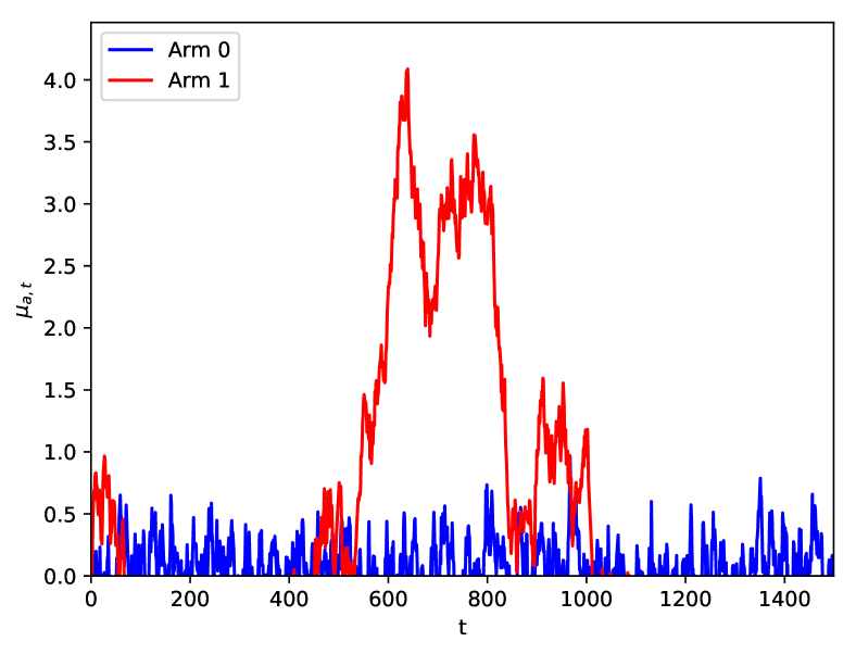
(a) Expected per-arm rewards over time for a contextual linear dynamic bandit with dynamics as in Eqn. (45). Note how the optimal arm switches around $t=\{50,500,900\}$, and how arm 0 becomes the best for $t\geq 1000$.

(b) Expected per-arm rewards over time for a contextual linear dynamic bandit with dynamics as in Eqn. (46). Note the optimal arm switches before $t=400$, and how arm 1 becomes the best for $t\geq 800$.

Figure 1: Expected per-arm rewards over time for different contextual linear dynamic bandit with dynamics as in Eqn. (21).

We consider this setting of special interest because the induced expected rewards change over time and so, the decision on the optimal arm swaps accordingly. We evaluate the proposed SIR-based methods for bandits with dynamics as in Eqns. (45)-(46), and both contextual linear-Gaussian and logistic rewards.

We show in Fig. 2 that the regret of SIR-based methods, for the contextual linear-Gaussian case with known parameters, is equivalent to the optimal case (i.e., the Kalman filter). Furthermore, even for cases when the reward variance $\sigma^{2}$ is unknown, and thus the Gaussianity assumption needs to be dropped (instead modeling bandit rewards via Student-t distributions), SIR-based methods perform comparably well.

(a) Expected per-arm rewards over time for Scenario A in Eqn. (45).

(b) Expected per-arm rewards over time for Scenario B in Eqn. (45).

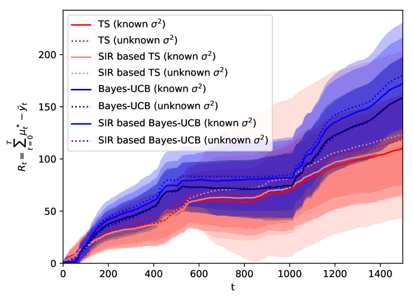
(c) Scenario A with known dynamic parameters.

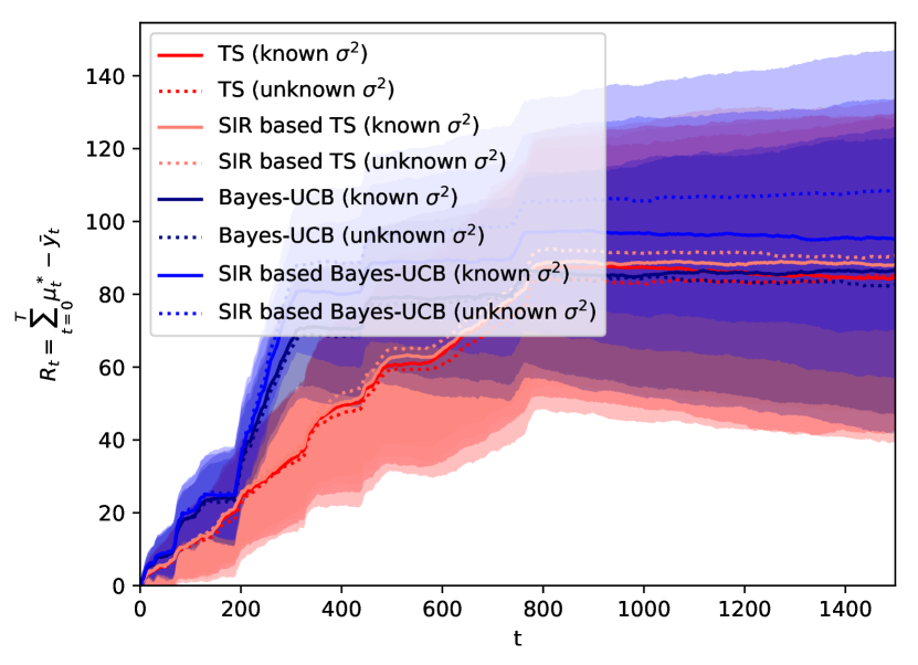
(d) Scenario B with known dynamic parameters.

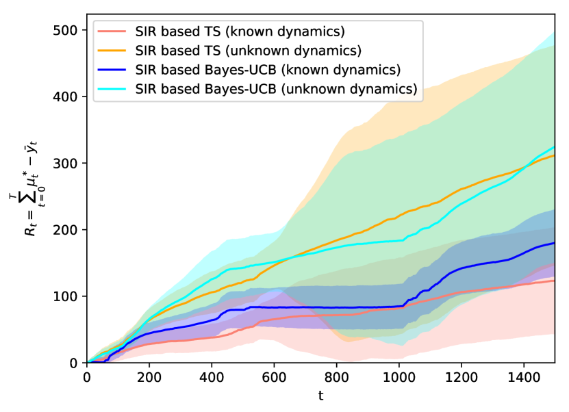
(e) Scenario A with unknown dynamic parameters.

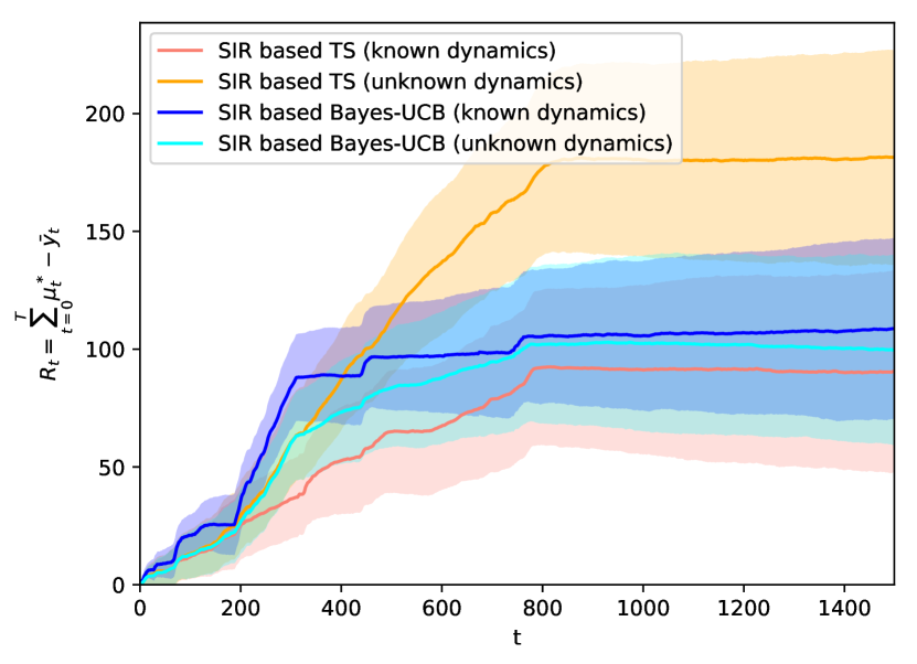
(f) Scenario B with unknown dynamic parameters.

Figure 2: Mean regret (standard deviation shown as shaded region) in contextual linear-Gaussian bandits with known dynamics. Notice the regret bumps when optimal arms swap, and how our proposed SIR-based methods adjust.

We further evaluate in Figs. 2(e) and  2(f) the most challenging contextual linear-Gaussian bandit case, where none of the parameters of the model ($L_{a},\Sigma_{a}$) are known; i.e., one must sequentially learn the underlying dynamics, in order to make informed online decisions.

(a) Expected per-arm rewards over time for Scenario A in Eqn. (45).

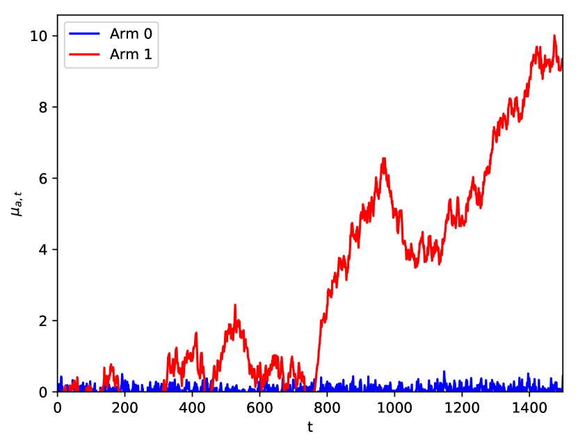
(b) Expected per-arm rewards over time for Scenario B in Eqn. (45).

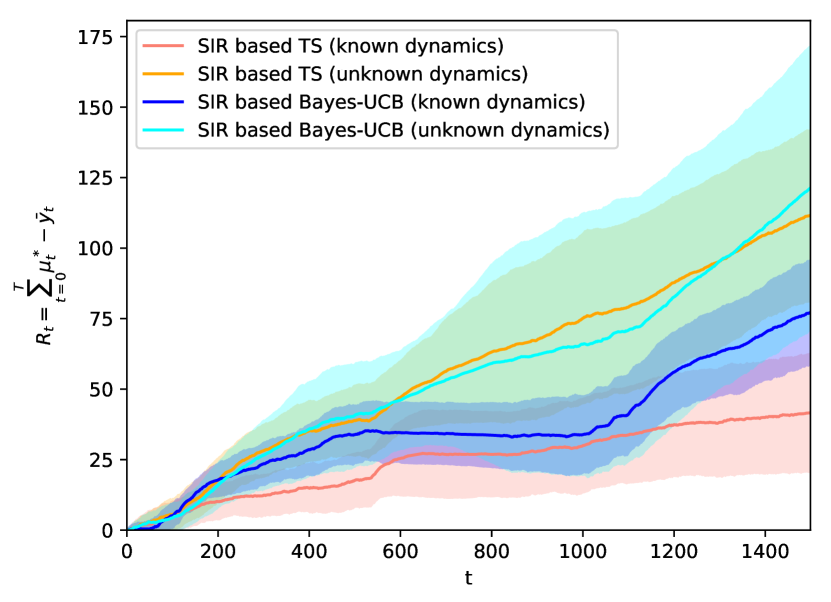
(c) Scenario A with known and unknown dynamic parameters.

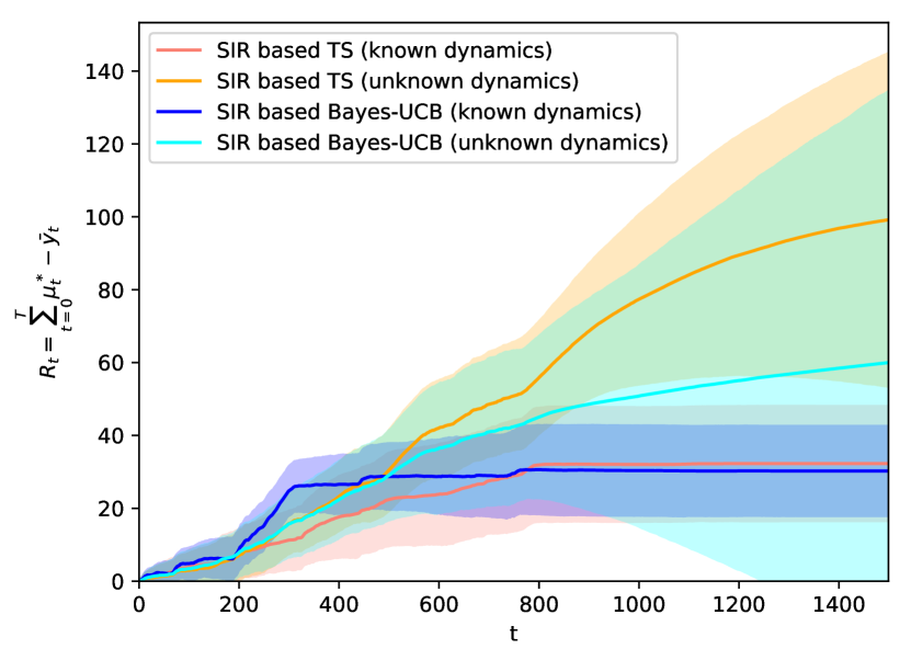
(d) Scenario B with known and unknown dynamic parameters.

Figure 3: Mean regret (standard deviation shown as shaded region) in contextual linear logistic dynamic bandits. Notice the regret bumps when optimal arms swap, and how our proposed SIR-based methods adjust.

Even if there is a regret performance loss due to the need to learn the unknown dynamic parameters, SIR-based Thompson sampling and Bayes-UCB are both able to learn their evolution and thus, reach the exploitation-exploration balance. We observe noticeable increases in regret when the dynamics of the parameters swap the optimal arm. This effect is also observed for dynamic bandits with non-Gaussian rewards. We evaluate our proposed framework with logistic reward functions with both static and random contexts: see regret performance in Fig. 3.

We now evaluate the proposed SIR-based framework with categorical multi-armed contextual dynamic bandits, which to the best of our knowledge, have not been studied before. We again leverage the time-varying dynamics of Eqn. (21), evaluated for different realizations of a diverse set of parameters.

We focus on two- and three-armed bandits, with numerical rewards $c=\{0,1,2\}$ dependent on a two-dimensional context $x_{t}\in{\mathbb{R}}^{2}$ with time-varying parameters $\theta_{a,c,t}$ as below:

$$\text{Two-armed bandit}\begin{split}\left(\begin{smallmatrix}\theta_{0,c,0,t}\\ \theta_{0,c,1,t}\\ \end{smallmatrix}\right)&=\left(\begin{smallmatrix}0.9&-0.1\\ -0.1&0.9\\ \end{smallmatrix}\right)\left(\begin{smallmatrix}\theta_{0,c,0,t-1}\\ \theta_{0,c,1,t-1}\\ \end{smallmatrix}\right)+\epsilon_{0,c},\;\forall c\in\{0,1,2\}\;,\\ \left(\begin{smallmatrix}\theta_{1,c,0,t}\\ \theta_{1,c,1,t}\\ \end{smallmatrix}\right)&=\left(\begin{smallmatrix}0.9&0.1\\ 0.1&0.9\\ \end{smallmatrix}\right)\left(\begin{smallmatrix}\theta_{1,c,0,t-1}\\ \theta_{1,c,1,t-1}\\ \end{smallmatrix}\right)+\epsilon_{1,c},\;\forall c\in\{0,1,2\}\;,\\ \text{ with i.i.d. }&\epsilon_{a,c}\sim\mathcal{N}\left(\epsilon|0,0.1\cdot\mathrm{I}\right)\forall a\in\{0,1\}\;,\forall c\in\{0,1,2\}\;.\end{split}$$ (47)

$$\text{Three-armed bandit}\begin{split}\left(\begin{smallmatrix}\theta_{0,c,0,t}\\ \theta_{0,c,1,t}\\ \end{smallmatrix}\right)&=\left(\begin{smallmatrix}0.9&-0.1\\ -0.1&0.9\\ \end{smallmatrix}\right)\left(\begin{smallmatrix}\theta_{0,c,0,t-1}\\ \theta_{0,c,1,t-1}\\ \end{smallmatrix}\right)+\epsilon_{0,c},\;\forall c\in\{0,1,2\}\;,\\ \left(\begin{smallmatrix}\theta_{1,c,0,t}\\ \theta_{1,c,1,t}\\ \end{smallmatrix}\right)&=\left(\begin{smallmatrix}0.9&0.1\\ 0.1&0.9\\ \end{smallmatrix}\right)\left(\begin{smallmatrix}\theta_{1,c,0,t-1}\\ \theta_{1,c,1,t-1}\\ \end{smallmatrix}\right)+\epsilon_{1,c},\;\forall c\in\{0,1,2\}\;,\\ \left(\begin{smallmatrix}\theta_{2,c,0,t}\\ \theta_{2,c,1,t}\\ \end{smallmatrix}\right)&=\left(\begin{smallmatrix}0.9&0.1\\ 0.1&0.9\\ \end{smallmatrix}\right)\left(\begin{smallmatrix}\theta_{2,c,0,t-1}\\ \theta_{2,c,1,t-1}\\ \end{smallmatrix}\right)+\epsilon_{2,c},\;\forall c\in\{0,1,2\}\;,\\ \text{ with i.i.d. }&\epsilon_{a,c}\sim\mathcal{N}\left(\epsilon|0,0.1\cdot\mathrm{I}\right)\forall a,c\in\{0,1,2\}\;.\end{split}$$ (48)

The parameterizations above accommodate a diverse set of expected reward dynamics, depending on parameter initializations, and realizations of the noise process. We illustrate the per-arm expected reward time-evolution for the studied two-armed bandit scenarios in Figures 4(a) and 4(b), and for the three-armed bandits, in Figures 5(a) and 5(b). We note that in all these settings, the expected rewards of each arm change over time, resulting in transient and recurrent swaps of the optimal arm.

We show the cumulative regret over time of Algorithm 1 in Figures 4(c), 4(d), 5(c) and 5(d), and observe that SMC-based Thompson sampling and Bayes-UCB are both able to reach the exploitation-exploration balance (the cumulative regret plateaus after optimal arm changes).

We observe increases in cumulative regret when the parameter dynamics swap the optimal arm — around $t\approx 1000$ in Fig 4(a), $t\approx 250$ and $t\approx 1600$ in Fig. 4(b), $t\approx 250$ in Fig. 5(a), $t\approx 250$ and $t\approx 1250$ in Fig. 5(b) — and how the SIR-based algorithms, via their updated dynamics, are able to readjust into a new exploitation-exploration balance.

We also observe that, when expected reward changes occur later in time (e.g., $t\approx 1750$ in Fig. 4(b) and $t\approx 1250$ in Fig. 5(b)), the impact on Bayes-UCB seems to be more pronounced: the mean increases drastically, as well as the variance (after $t\approx 1600$ in Fig. 4(d), and $t\approx 1250$ in Fig. 5(d)).

In the most interesting and challenging setting — those with time-evolving unknown parameters — both algorithms incur in an increased regret loss. Since the algorithm must sequentially learn the unknown model parameters $\{L_{a,c},C_{a,c}\}$ of the transition density that SMC uses, making informed decisions becomes more troublesome, thus the reward loss.

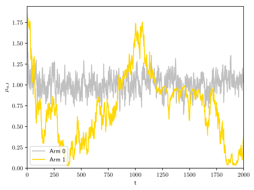
(a) Two-armed bandit expected reward time-evolution: notice the optimal arm change around $t\approx 1000$.

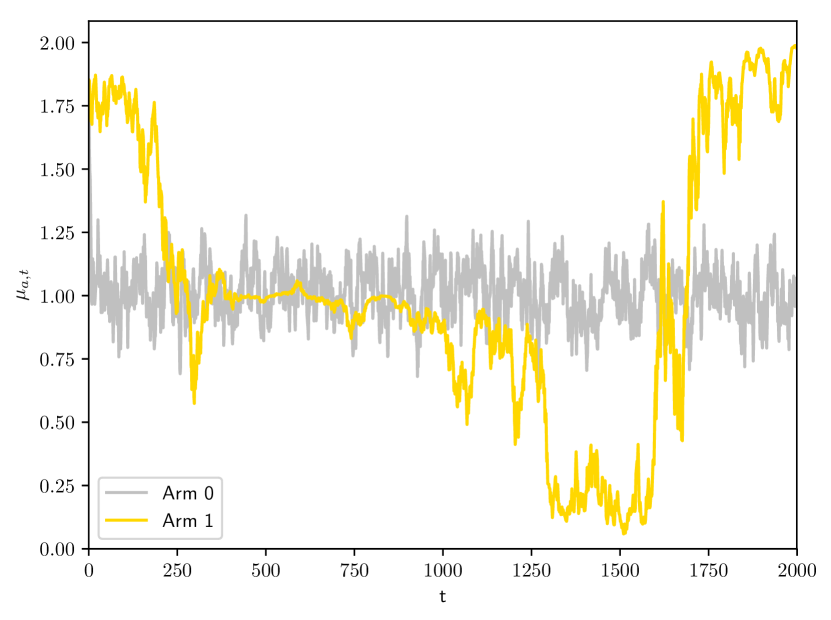
(b) Two-armed bandit expected reward time-evolution: notice the late optimal arm change around $t\approx 1600$.

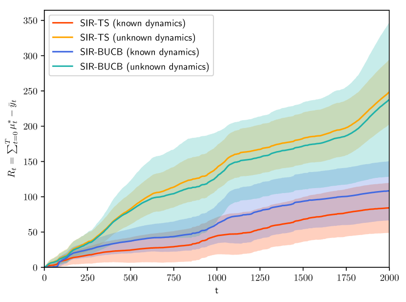
(c) Cumulative regret over time for a two-armed bandit with expected reward dynamics as above (Fig. 4(a)).

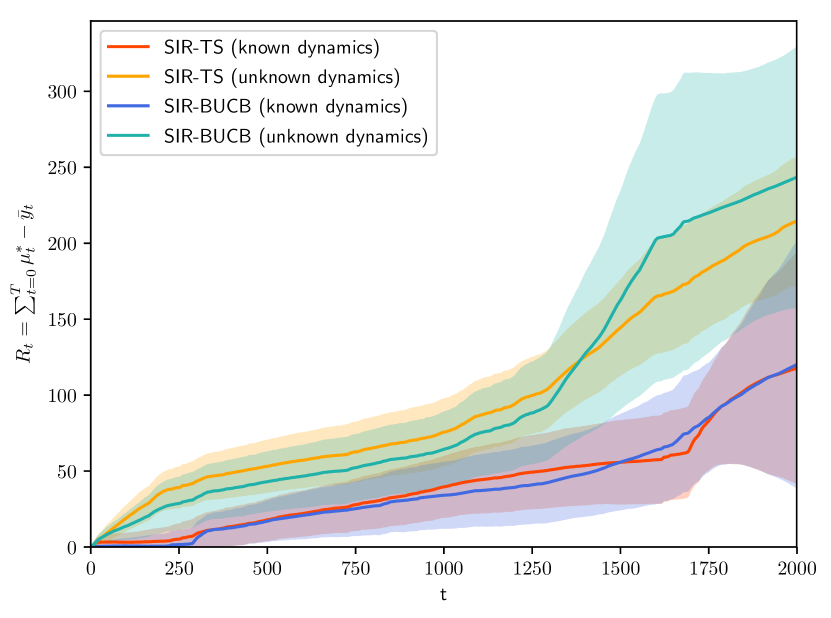
(d) Cumulative regret over time for a two-armed bandit with expected reward dynamics as above (Fig. 4(b)).

Figure 4: Expected reward time-evolution, and mean regret (standard deviation shown as shaded region) of the proposed methods, for a two-armed contextual three-categorical dynamic bandits as in Eqn. 47.

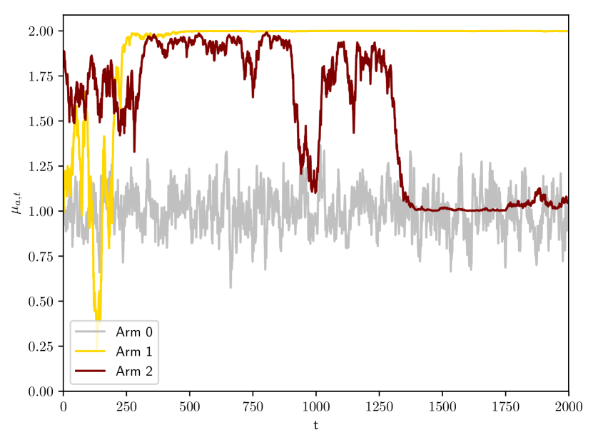
(a) Three-armed bandit expected reward time-evolution: notice the optimal arm change around $t\approx 250$.

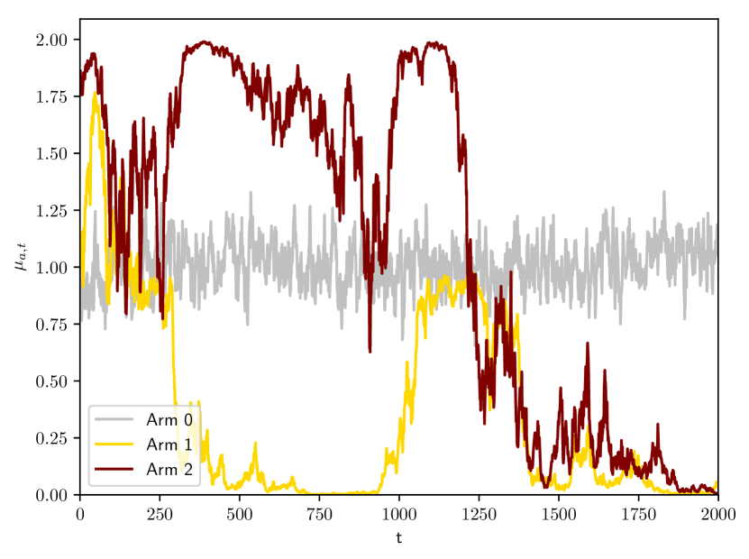
(b) Three-armed bandit expected reward time-evolution: notice the optimal arm changes around $t\approx 250$ and $t\approx 1250$.

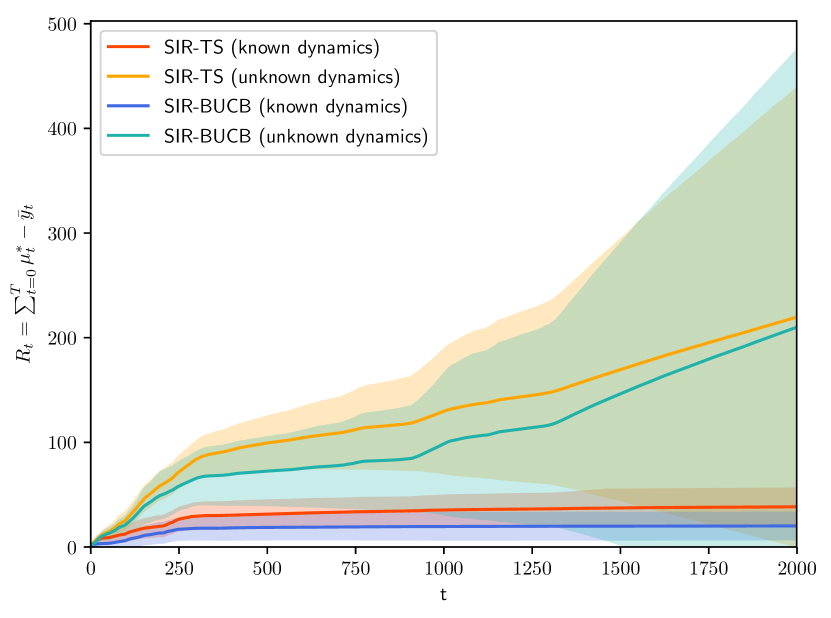
(c) Cumulative regret over time for a three-armed bandit with expected reward dynamics as above (Fig. 5(a)).

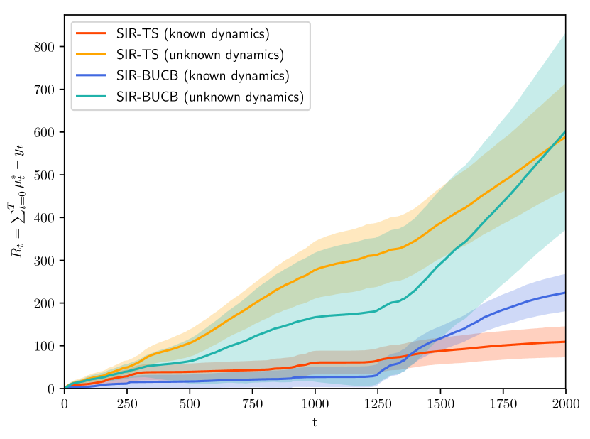
(d) Cumulative regret over time for a three-armed bandit with expected reward dynamics as above (Fig. 5(b)).

Figure 5: Expected reward time-evolution, and mean regret (standard deviation shown as shaded region) of the proposed methods, for a three armed contextual three-categorical dynamic bandits as in Eqn. 48.

Overall, the random measure approximation to the posteriors of the parameters of interest is accurate enough, allowing both studied MAB policies to dynamically find and adjust to the right exploration-exploitation tradeoff in all the studied dynamic bandits (Gaussian, logistic and categorical).

The proposed SMC-based framework not only estimates the evolving parameters $\theta_{t}$, but also their corresponding uncertainty. Both because an arm’s dynamics are unclear, or due to an arm not being sampled for a while, the uncertainty of its estimated SMC posterior grows. As a result, a Bayesian policy is more likely to explore that arm again.

We observe a slightly deteriorating behavior over time for Bayes-UCB in all studied cases, which we argue is due to the shrinking quantile value $\alpha_{t}\propto 1/t$, originally proposed by Kaufmann et al. (46). Confidence bounds of static reward models tend to shrink with more observations of the bandit. However, with evolving parameters, such assumption does not hold anymore. The uncertainty of the evolving parameter posteriors (driven by the underlying dynamics of each arms) might result in broader distributions. Therefore, the inadequacy of shrinking $\alpha_{t}$, as it is not able to capture the evolving uncertainty of the parameter posteriors in the long run. More generally, the need to determine appropriate quantile values $\alpha_{t}$ for each reward and dynamic model is a drawback for Bayes-UCB, as its optimal value will depend on the specific combination of underlying dynamics and reward function.

On the contrary, Thompson sampling relies on samples from the posterior, which SMC methods are able to approximate accurately enough in all studied cases for it to operate successfully without any parameter tweaking.

4.1 Bandits for personalized news article recommendation

Finally, we consider the application of the proposed SIR-based methods for recommendation of personalized news articles, in a similar fashion as done by Chapelle and Li (18). Online content recommendation represents an important example of reinforcement learning, as it requires efficient balancing of the exploration and exploitation tradeoff.

We use a dataset that contains a fraction of user click logs for news articles displayed in the Featured Tab of the Today Module on Yahoo! Front Page during the first ten days in May 2009. The articles to be displayed were originally chosen uniformly at random from a hand-picked pool of high-quality articles. As such, the candidate pool was originally dynamic. However, we picked a subset of 20 articles shown in May 06th and collected all logged user interactions, for a total of 500354.

The goal is to choose the most interesting article to users, or in bandit terms, to maximize the total number of clicks on the recommended articles, i.e., the average click-through rate (CTR). In the dataset, each user is associated with six features: a bias term and 5 features that correspond to the membership features constructed via the conjoint analysis with a bilinear model described in (22).

We treat each article as an arm ($A=20$), and the logged reward is whether the article is clicked or not by the user ($y_{t}=\{1,0\}$). We pose the problem as a MAB with logistic rewards, so that we can account for the user features ($x_{t}\in{\mathbb{R}}^{6}$).

One may further hypothesize that the news recommendation system should evolve over time, as the relevance of news might change during the course of the day. As a matter of fact, our proposed framework readily accommodates these assumptions.

We consider both static and dynamic bandits with logistic rewards, and implement the proposed SIR-based Thompson sampling, due to its flexibility and the lack of parameter tuning required. Summary CTR results are provided in Table 1. Observe the flexibility of the dynamic bandit in Fig. 6, which is able to pick up the dynamic popularity of certain articles over time.

Figure 6: Empirical probability of SIR-based contextual dynamic logistic Thompson sampling policy picking each arm over time. Notice how the algorithm captures the changing popularity of articles over time.

		CTR	Normalized CTR
	Logistic rewards, static arms	0.0670 +/- 0.0088	1.6095 +/- 0.2115
	Logistic rewards, time-evolving arms	0.0655 +/- 0.0082	1.5745 +/- 0.2064
Model

Table 1: CTR results for SIR-based bandits on the news article recommendation data. The normalized CTR is with respect to a random baseline.

5 Conclusion

We have presented a (sequential) importance sampling-based framework for the MAB problem, where we combine sequential Monte Carlo inference with state-of-the-art Bayesian MAB policies. The proposed algorithmic setting allows for interpretable modeling of complex reward functions and time-evolving bandits. The methods sequentially learn the dynamics of the bandit from online data, and are able to find the exploration-exploitation balance.

In summary, we extend the applicability of Bayesian MAB policies (Thompson sampling and Bayes-UCB in particular) by accommodating complex models of the world with SIR-based inference of the unknowns. Empirical results show good cumulative regret performance of the proposed framework in simulated challenging models (e.g., contextual categorical dynamic bandits), and practical scenarios (personalized news article recommendation) where complex models of data are required.

Important future work remains on a deeper understanding of the regret of both Thompson sampling and UCB-based policies within the proposed SMC-based framework. A theoretical analysis of the dependency between optimal arm changes, posterior convergence, and regret of the proposed SMC-based framework must be devised.

5.1 Software and Data

The implementation of the proposed method is available in this public repository. It contains all the software required for replication of the findings of this study.

Acknowledgments

This research was supported in part by NSF grant SCH-1344668. We thank Luke Bornn for bringing (19) to our attention.

Appendix A MAB models

We now describe the key distributions for some MAB models of interest.

A.1 SIR for static bandits

These are bandits where there are no time-varying parameters: i.e., $\theta_{t}=\theta,\forall t$. For these settings, SIR-based parameter propagation becomes troublesome (60), and to mitigate such issues, several alternatives have been proposed in the SMC community: artificial parameter evolution (40), kernel smoothing (60), and density assisted techniques (28).

We resort to density assisted importance sampling, rather than to kernel based particle filters as implemented in (19), where one approximates the posterior of the unknown parameters with a density of choice. Density assisted importance sampling is a well studied SMC approach that extends random-walking and kernel-based alternatives (40, 59, 28), with its asymptotic correctness guaranteed for the static parameter case.

Specifically, we approximate the posterior of the unknown parameters $\theta$, given the current state of knowledge, with a Gaussian distribution $p(\theta_{a}|\mathcal{H}_{1:t})\approx\mathcal{N}\left(\theta_{a}|\hat{\theta}_{t,a},\hat{\Sigma}_{\theta_{t,a}}\right)$. The sufficient statistics are computed based on samples and weights of the random measure $p_{M}(\theta_{t,a})=\sum_{m=1}^{M}w_{t}^{(m)}\delta\left(\theta_{t,a}-\theta_{t,a}^{(m)}\right)$ available at each time instant:

$$\begin{split}\hat{\theta}_{t,a}&=\sum_{i=1}^{M}w_{t,a}^{(m)}\theta^{(m)}_{t,a}\;,\\ \hat{\Sigma}_{\theta_{t,a}}&=\sum_{i=1}^{M}w_{t,a}^{(m)}(\theta^{(m)}_{t,a}-\hat{\theta}_{t,a})(\theta^{(m)}_{t,a}-\hat{\theta}_{t,a})^{\top}\;.\end{split}$$ (49)

For static bandits, when propagating parameters in Algorithm 1, one draws from $p(\theta_{t+1,a}|\theta_{t,a})=p(\theta_{t,a}|\mathcal{H}_{1:t})\approx\mathcal{N}\left(\theta_{t,a}|\hat{\theta}_{t,a},\hat{\Sigma}_{\theta_{t,a}}\right)$.

A.2 Linearly dynamic bandits

Let us consider a general linear model for the dynamics of the parameters of each arm $\theta_{a}\in{\mathbb{R}}^{d}$:

$$\theta_{t,a}=L_{a}\theta_{t-1,a}+\epsilon_{a}\;,\qquad\epsilon_{a}\sim\mathcal{N}\left(\epsilon_{a}|0,\Sigma_{a}\right)\;,$$ (50)

where $L_{a}\in{\mathbb{R}}^{d\times d}$ and $\Sigma_{a}\in{\mathbb{R}}^{d\times d}$. One can immediately determine that, for linearly dynamic bandits with known parameters, the parameters follow

$$\theta_{t,a}\sim\mathcal{N}\left(\theta_{t,a}|L_{a}\theta_{t-1,a},\Sigma_{a}\right)\;.$$ (51)

However, it is unrealistic to assume that the parameters are known in practice. We thus marginalize them out by means of the following conjugate priors for the matrix $L$ and covariance matrix $\Sigma$ (we drop the per arm subscript $a$ for clarity)

$$\begin{split}p(L,\Sigma|L_{0},B_{0},\nu_{0},V_{0})&={\rm NIW}\left(L,\Sigma|L_{0},B_{0},\nu_{0},V_{0}\right)=p(L|L_{0},B_{0},\Sigma)p(\Sigma|\nu_{0},V_{0})\\ &=\mathcal{MN}\left(L|L_{0},\Sigma,B_{0}\right){\rm IW}\left(\Sigma|\nu_{0},V_{0}\right)\;,\end{split}$$ (52)

where the matrix variate Gaussian distribution follows

$$\mathcal{MN}\left(L|L_{0},\Sigma,B_{0}\right)=\frac{e^{-\frac{1}{2}\mathrm{tr}\left\{B_{0}^{-1}\left(L-L_{0}\right)^{\top}\Sigma^{-1}\left(L-L_{0}\right)\right\}}}{(2\pi)^{(d\cdot d)/2}\left|B_{0}\right|^{d/2}\left|\Sigma\right|^{d/2}}\;,$$ (53)

and the Inverse Wishart

$${\rm IW}\left(\Sigma|\nu_{0},V_{0}\right)=\frac{\left|\Sigma\right|^{-\frac{\nu_{0}+d+1}{2}}e^{-\frac{1}{2}\mathrm{tr}\left\{\Sigma^{-1}V_{0}\right\}}}{2^{\frac{\nu_{0}\cdot d}{2}}\left|V_{0}\right|^{-\frac{\nu_{0}}{2}}\Gamma\left(\frac{\nu_{0}}{2}\right)}\;.$$ (54)

We integrate out the unknown parameters $L$ and $\Sigma$ to derive the predictive density, i.e., the distribution of $\theta_{t}$, given all the past data $\theta_{1:t}$. One can show that the resulting distribution is a multivariate t-distribution

$$\begin{split}f(\theta_{t}|\theta_{1:t-1})&=\mathcal{T}\left(\theta_{t}|\nu_{t},m_{t},R_{t}\right)\propto\left|1+\frac{1}{\nu_{t}}\left(\theta_{t}-m_{t}\right)R_{t}^{-1}\left(\theta_{t}-m_{t}\right)^{\top}\right|^{-\frac{\nu_{t}+d}{2}}\;,\end{split}$$ (55)

where $\nu_{t}$ denotes degrees of freedom, $m_{t}\in{\mathbb{R}}^{d}$ is the location parameter, and $R_{t}\in{\mathbb{R}}^{d\times d}$ represents the scale matrix (10). These follow

$$\begin{cases}\nu_{t}=\nu_{0}+t-d\;,\\ m_{t}=L_{t-1}\theta_{t-1}\;,\\ R_{t}=\frac{V_{t-1}}{\nu_{t}\left(1-\theta_{t-1}^{\top}(UU^{\top})^{-1}\theta_{t-1}\right)}\;,\\ \end{cases}$$ (56)

where the sufficient statistics of the parameters are

$$\begin{cases}B_{t-1}=\left(\Theta_{0:t-2}\Theta_{0:t-2}^{\top}+B_{0}^{-1}\right)^{-1}\;,\\ L_{t-1}=\left(\Theta_{1:t-1}\Theta_{0:t-2}^{\top}+L_{0}B_{0}^{-1}\right)B_{t-1}\;,\\ V_{t-1}=\left(\Theta_{1:t-1}-L_{t-1}\Theta_{0:t-2}\right)\left(\Theta_{1:t-1}-L_{t-1}\Theta_{0:t-2}\right)^{\top}\\ \qquad\qquad+\left(L_{t-1}-L_{0}\right)B_{0}^{-1}\left(L_{t-1}-L_{0}\right)^{\top}+V_{0}\;,\\ UU^{\top}=\left(\theta_{t-1}\theta_{t-1}^{\top}+B_{t-1}^{-1}\right)\;,\\ \end{cases}$$ (57)

and we have defined the stacked parameter matrix

$$\Theta_{t_{0}:t_{1}}=[\theta_{t_{0}}\theta_{t_{0}+1}\cdots\theta_{t_{1}-1}\theta_{a,t_{1}}]\in{\mathbb{R}}^{d\times(t_{1}-t_{0})}\;.$$ (58)

All in all, for linear dynamic bandits with unknown parameters, the per-arm parameters follow

$$\theta_{t,a}\sim\mathcal{T}\left(\theta_{t,a}|\nu_{t,a},m_{t,a},R_{t,a}\right)\;.$$ (59)

Appendix B Evaluation

In the following pages, we provide results for many parameterizations of the evaluated bandits, both for the static and dynamic cases

B.1 Static bandits

We first compare the performance of Algorithm 1 to Thompson sampling (TS) and Bayes-UCB in their original formulations: static bandits with Bernoulli and contextual linear-Gaussian reward functions.

We provide results for bandits with 2,3, and 5 arms for Bernoulli rewards in Sections B.1.1, B.1.2, B.1.3, and contextual-Gaussian rewards in Sections B.1.4, B.1.5, B.1.6, where we show how the proposed SIR-based algorithm perform similarly to the benchmark policies with analytical posteriors. We also evaluate a more realistic scenario for the contextual linear-Gaussian case with unknown reward variance $\sigma^{2}$, where SIR-based approaches are shown to be competitive as well.

Note the increased uncertainty due to the MC approximation to the posterior, which finds its analytical justification in Eqn. (9), and can be empirically reduced by increasing the number $M$ of IS samples used (see the impact of sample size $M$ in the provided figures). In general, $M=1000$ samples suffice in all our experiments for accurate estimation of parameter posteriors. Advanced and dynamic determination of SIR sample size is an active research area within the SMC community, but out of the scope of this paper.

In several applications, binary rewards are well-modeled as depending on contextual factors (18, 78). The logistic reward function is suitable for these scenarios but, due to the unavailability of Bayesian closed-form posterior updates, one needs to resort to approximations, e.g., the ad-hoc Laplace approximation proposed by Chapelle and Li (18).

Our proposed SIR-based framework is readily applicable, as one only needs to evaluate the logistic reward likelihood to compute the IS weights for the MAB policy of choice. Results in Sections B.1.7, B.1.8, B.1.9 show how quickly SIR-based Thompson sampling and Bayes-UCB achieve the right exploration-exploitation tradeoff for different logistic parameterizations.

These results indicate that the impact of only observing rewards of the played arms is minimal for the proposed SIR-based method. The parameter posterior uncertainty associated with the SIR-based estimation is automatically accounted for by both algorithms, as they explore rarely-played arms if the uncertainty is high. However, we do observe a slight performance deterioration of Bayes-UCB, which we argue is related to the quantile value used ($\alpha_{t}\propto 1/t$). It was analytically justified by Kaufmann (46) for Bernoulli rewards, but might not be optimal for other reward functions and, more importantly, for the SIR-based approximation to parameter posteriors. On the contrary, Thompson sampling is more flexible, automatically adjusting to the uncertainty of the posterior approximation, and thus, attaining reduced regret.

B.1.1 Bernoulli bandits, A=2

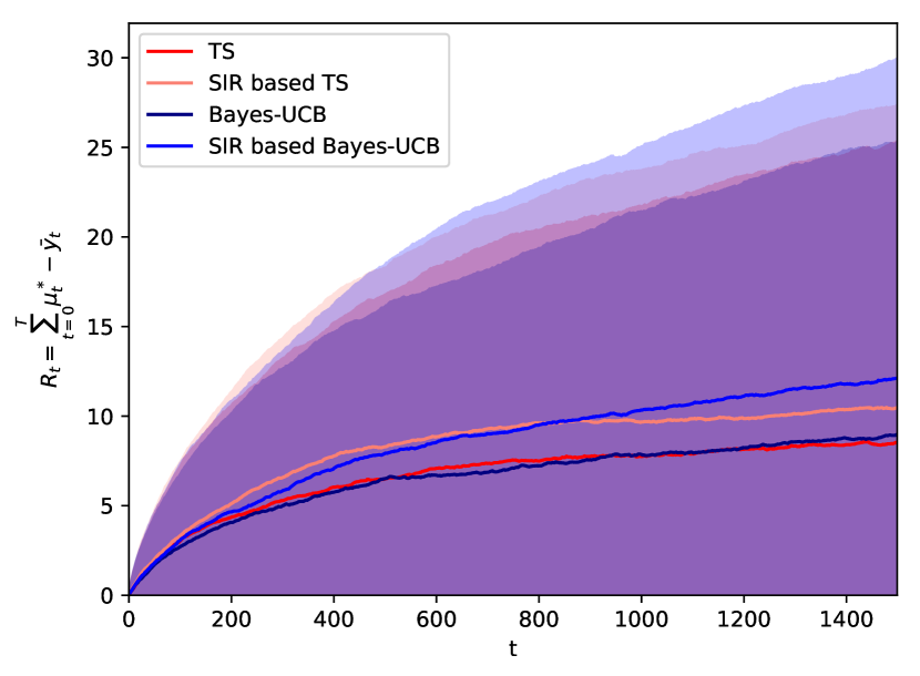
(a) Bernoulli bandit, $\theta_{0}=0.1,\theta_{1}=0.2$.

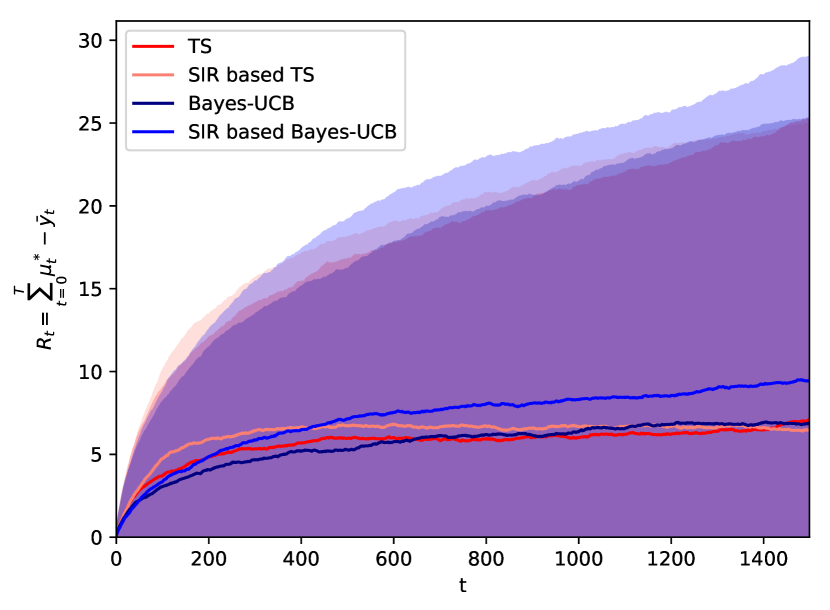
(b) Bernoulli bandit, $\theta_{0}=0.1,\theta_{1}=0.3$.

(c) Bernoulli bandit, $\theta_{0}=0.5,\theta_{1}=0.6$.

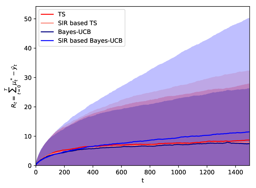
(d) Bernoulli bandit, $\theta_{0}=0.5,\theta_{1}=0.7$.

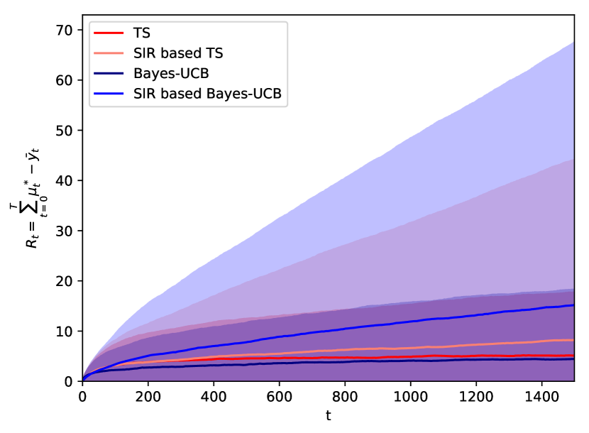
(e) Bernoulli bandit, $\theta_{0}=0.7,\theta_{1}=0.9$.

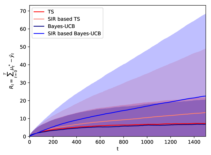
(f) Bernoulli bandit, $\theta_{0}=0.8,\theta_{1}=0.9$.

Figure 7: Mean regret (standard deviation shown as shaded region) in static two-armed Bernoulli bandits.

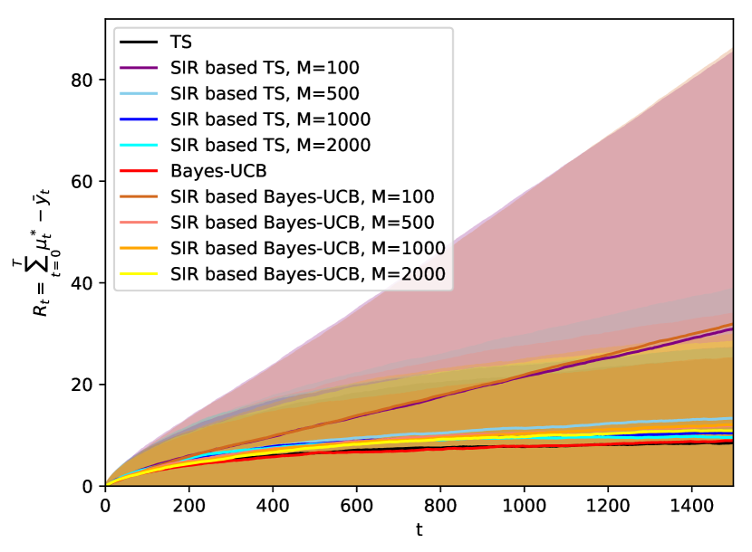
(a) Bernoulli bandit, $\theta_{0}=0.1,\theta_{1}=0.2$.

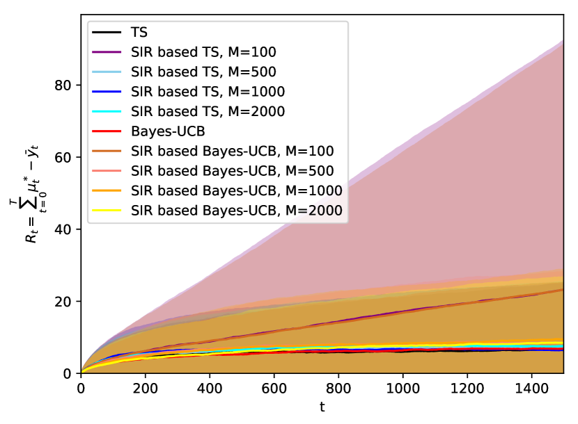
(b) Bernoulli bandit, $\theta_{0}=0.1,\theta_{1}=0.3$.

(c) Bernoulli bandit, $\theta_{0}=0.5,\theta_{1}=0.6$.

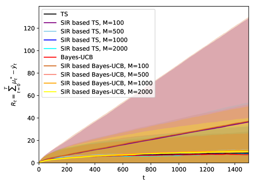
(d) Bernoulli bandit, $\theta_{0}=0.5,\theta_{1}=0.7$.

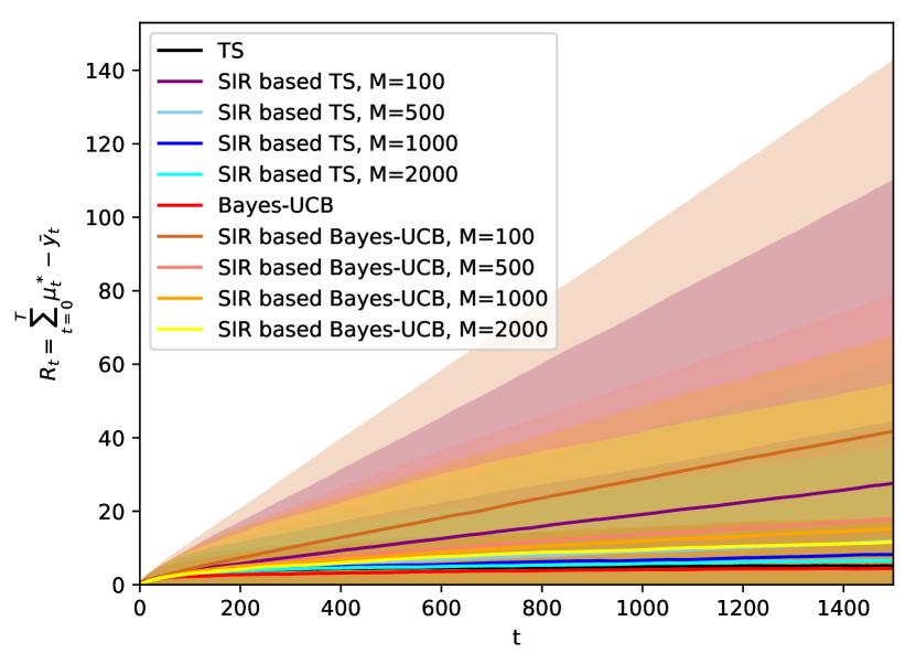
(e) Bernoulli bandit, $\theta_{0}=0.7,\theta_{1}=0.9$.

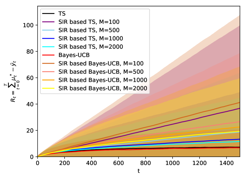
(f) Bernoulli bandit, $\theta_{0}=0.8,\theta_{1}=0.9$.

Figure 8: Mean regret (standard deviation shown as shaded region) in static two-armed Bernoulli bandits.

B.1.2 Bernoulli bandits, A=3

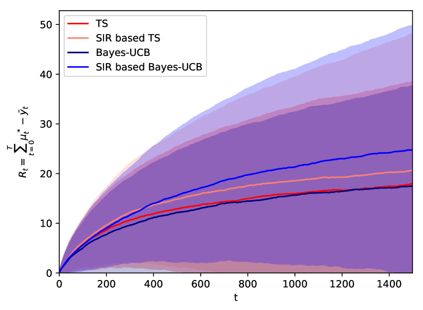
(a) Bernoulli bandit, $\theta_{0}=0.1,\theta_{1}=0.2,\theta_{2}=0.3$.

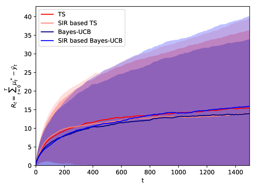
(b) Bernoulli bandit, $\theta_{0}=0.1,\theta_{1}=0.3,\theta_{2}=0.5$.

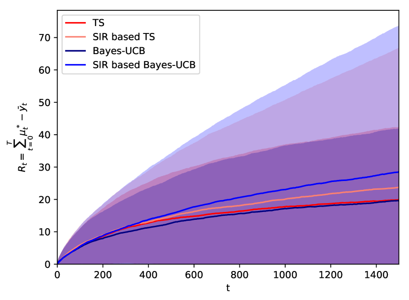
(c) Bernoulli bandit, $\theta_{0}=0.5,\theta_{1}=0.6,\theta_{2}=0.7$.

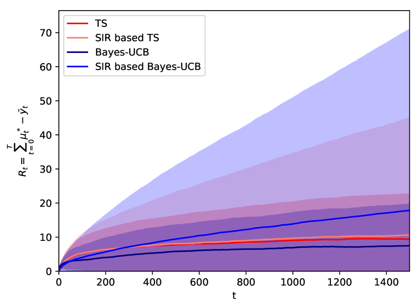
(d) Bernoulli bandit, $\theta_{0}=0.5,\theta_{1}=0.7,\theta_{2}=0.9$.

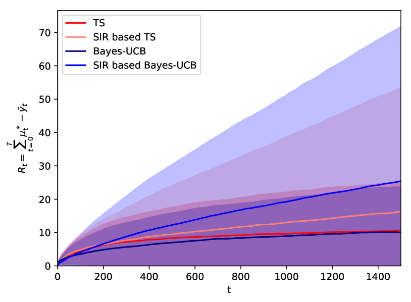
(e) Bernoulli bandit, $\theta_{0}=0.5,\theta_{1}=0.8,\theta_{2}=0.9$.

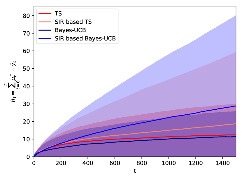
(f) Bernoulli bandit, $\theta_{0}=0.7,\theta_{1}=0.8,\theta_{2}=0.9$.

Figure 9: Mean regret (standard deviation shown as shaded region) in static three-armed Bernoulli bandits.

(a) Bernoulli bandit, $\theta_{0}=0.1,\theta_{1}=0.2,\theta_{2}=0.3$.

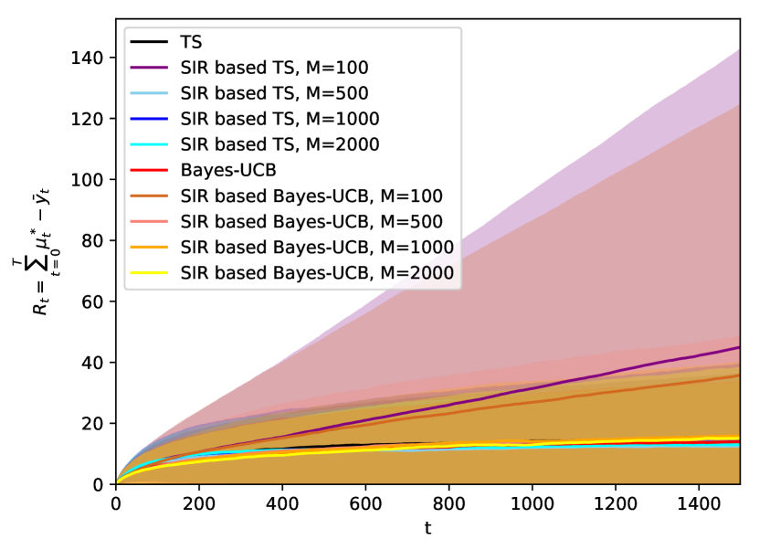
(b) Bernoulli bandit, $\theta_{0}=0.1,\theta_{1}=0.3,\theta_{2}=0.5$.

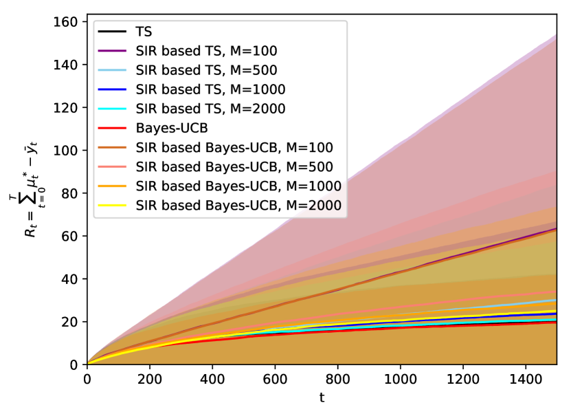
(c) Bernoulli bandit, $\theta_{0}=0.5,\theta_{1}=0.6,\theta_{2}=0.7$.

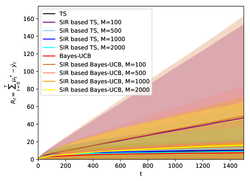
(d) Bernoulli bandit, $\theta_{0}=0.5,\theta_{1}=0.7,\theta_{2}=0.9$.

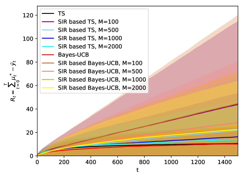
(e) Bernoulli bandit, $\theta_{0}=0.5,\theta_{1}=0.8,\theta_{2}=0.9$.

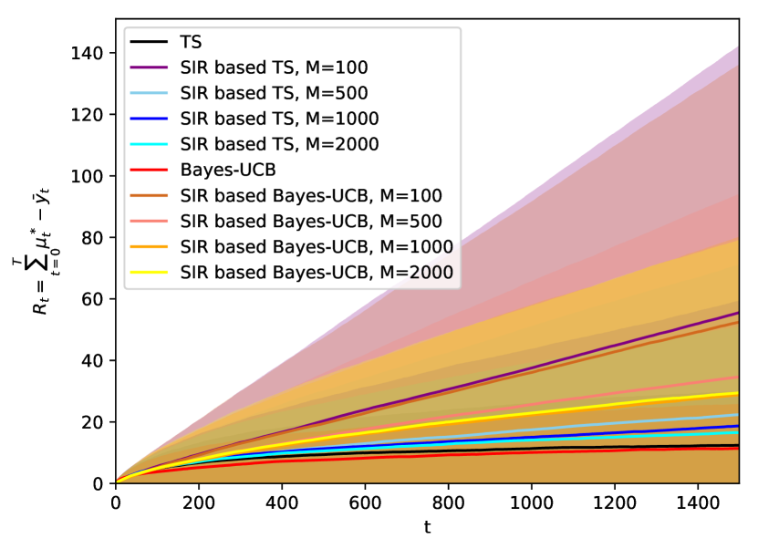
(f) Bernoulli bandit, $\theta_{0}=0.7,\theta_{1}=0.8,\theta_{2}=0.9$.

Figure 10: Mean regret (standard deviation shown as shaded region) in static three-armed Bernoulli bandits.

B.1.3 Bernoulli bandits, A=5

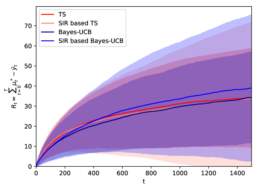
(a) Bernoulli bandit, $\theta_{0}=0.1,\theta_{1}=0.2,\\ \theta_{2}=0.3,\theta_{3}=0.4,\theta_{4}=0.5$.

(b) Bernoulli bandit, $\theta_{0}=0.1,\theta_{1}=0.3,\\ \theta_{2}=0.5,\theta_{3}=0.6,\theta_{4}=0.8$.

(c) Bernoulli bandit, $\theta_{0}=0.1,\theta_{1}=0.3,\\ \theta_{2}=0.5,\theta_{3}=0.8,\theta_{4}=0.9$.

(d) Bernoulli bandit, $\theta_{0}=0.1,\theta_{1}=0.5,\\ \theta_{2}=0.6,\theta_{3}=0.7,\theta_{4}=0.9$.

(e) Bernoulli bandit, $\theta_{0}=0.3,\theta_{1}=0.4,\\ \theta_{2}=0.5,\theta_{3}=0.7,\theta_{4}=0.9$.

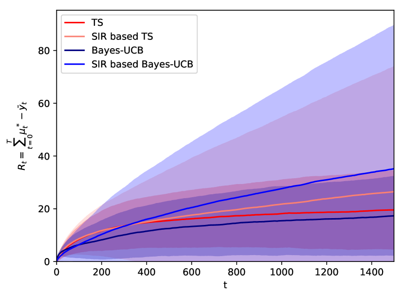
(f) Bernoulli bandit, $\theta_{0}=0.5,\theta_{1}=0.6,\\ \theta_{2}=0.7,\theta_{3}=0.8,\theta_{4}=0.9$.

Figure 11: Mean regret (standard deviation shown as shaded region) in static five-armed Bernoulli bandits.

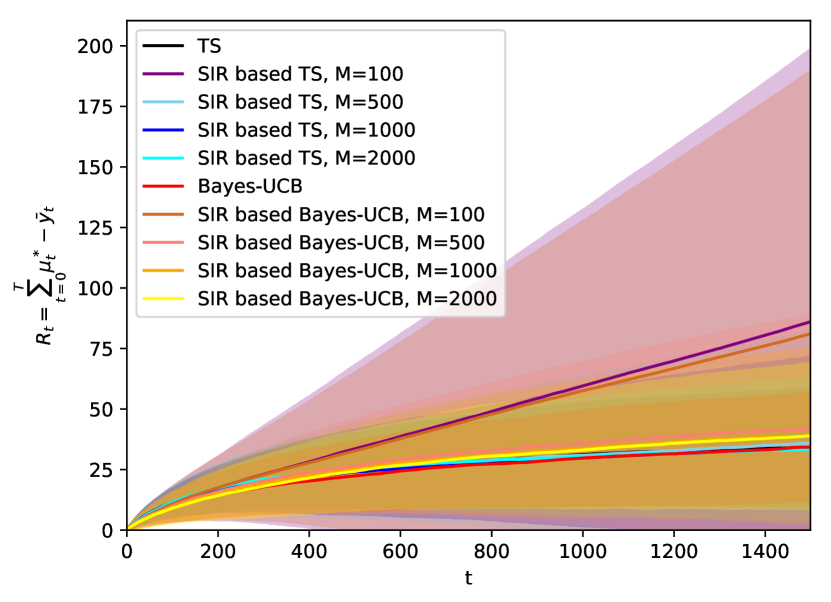
(a) Bernoulli bandit, $\theta_{0}=0.1,\theta_{1}=0.2,\\ \theta_{2}=0.3,\theta_{3}=0.4,\theta_{4}=0.5$.

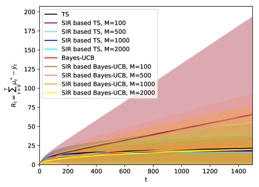
(b) Bernoulli bandit, $\theta_{0}=0.1,\theta_{1}=0.3,\\ \theta_{2}=0.5,\theta_{3}=0.6,\theta_{4}=0.8$.

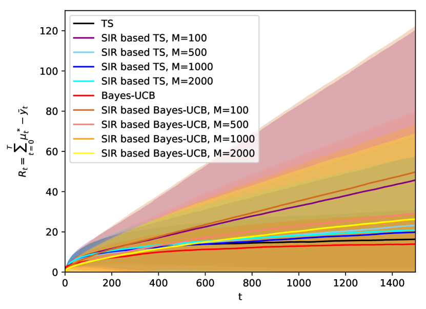
(c) Bernoulli bandit, $\theta_{0}=0.1,\theta_{1}=0.3,\\ \theta_{2}=0.5,\theta_{3}=0.8,\theta_{4}=0.9$.

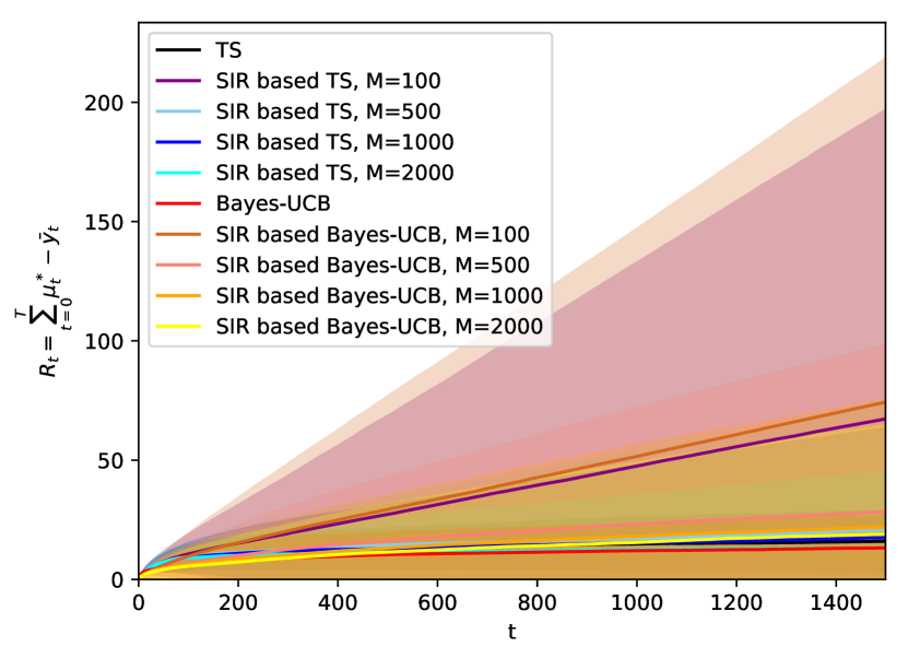
(d) Bernoulli bandit, $\theta_{0}=0.1,\theta_{1}=0.5,\\ \theta_{2}=0.6,\theta_{3}=0.7,\theta_{4}=0.9$.

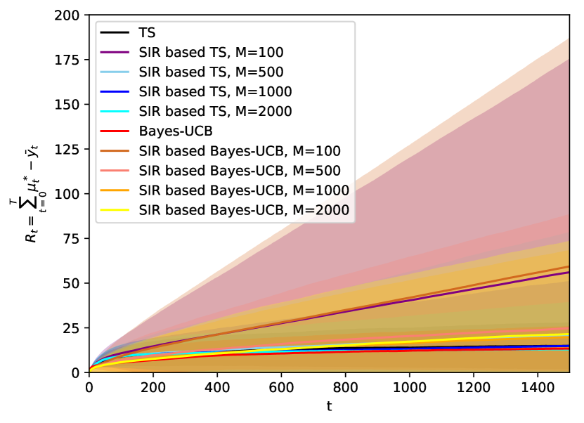
(e) Bernoulli bandit, $\theta_{0}=0.3,\theta_{1}=0.4,\\ \theta_{2}=0.5,\theta_{3}=0.7,\theta_{4}=0.9$.

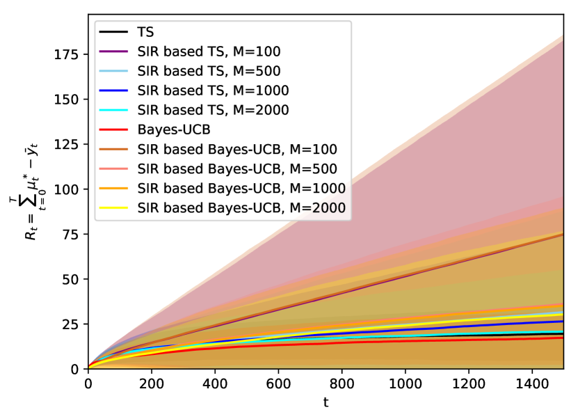
(f) Bernoulli bandit, $\theta_{0}=0.5,\theta_{1}=0.6,\\ \theta_{2}=0.7,\theta_{3}=0.8,\theta_{4}=0.9$.

Figure 12: Mean regret (standard deviation shown as shaded region) in static five-armed Bernoulli bandits.

B.1.4 Contextual Linear Gaussian bandits, A=2

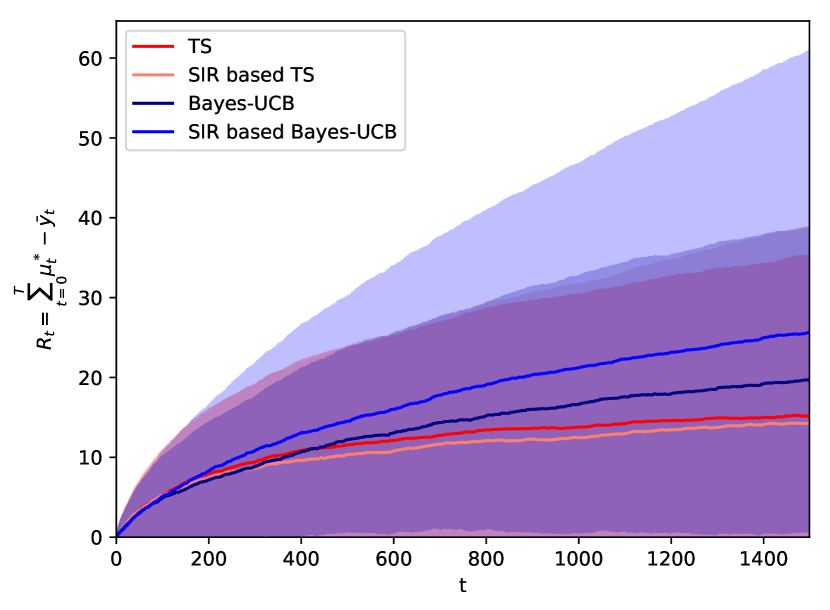
(a) Contextual Gaussian bandit,
$\theta_{0}=(-0.1,-0.1),\theta_{1}=(0.1,0.1),\sigma^{2}=0.5$.

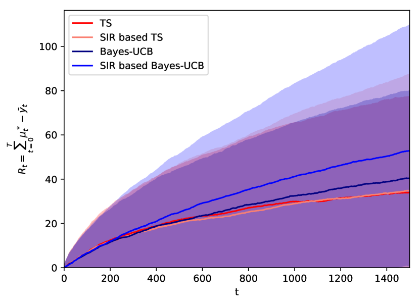
(b) Contextual Gaussian bandit,
$\theta_{0}=(-0.1,-0.1),\theta_{1}=(0.1,0.1),\sigma^{2}=1.0$.

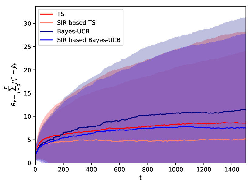
(c) Contextual Gaussian bandit,
$\theta_{0}=(-0.5,-0.5),\theta_{1}=(0.5,0.5),\sigma^{2}=0.5$.

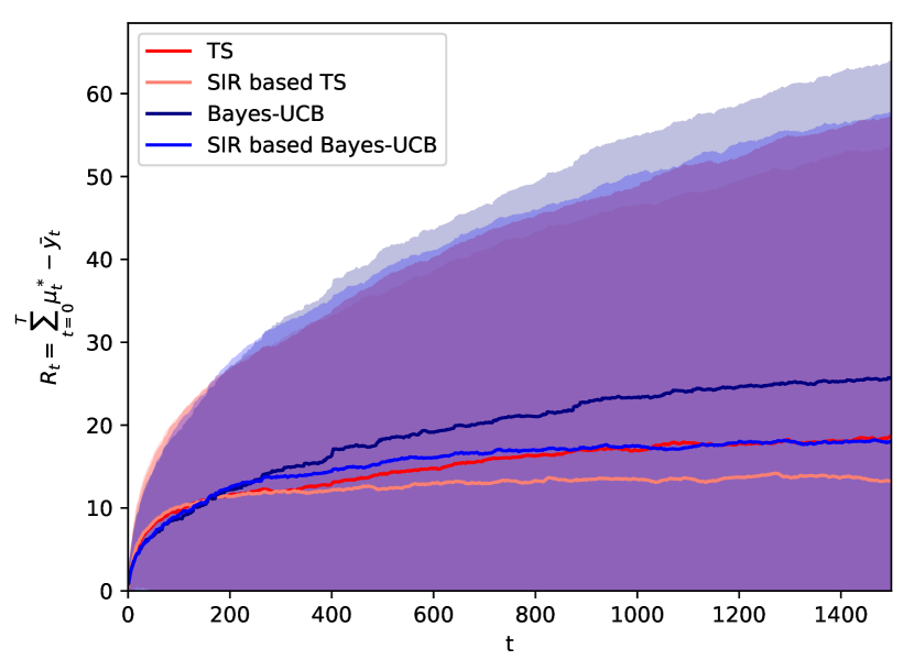
(d) Contextual Gaussian bandit,
$\theta_{0}=(-0.5,-0.5),\theta_{1}=(0.5,0.5),\sigma^{2}=1.0$.

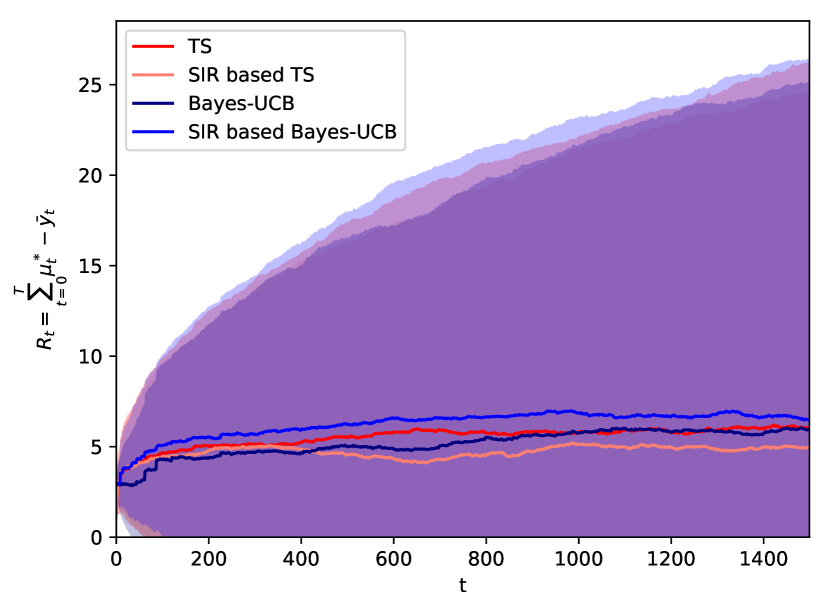
(e) Contextual Gaussian bandit,
$\theta_{0}=(-1,-1),\theta_{1}=(1,1),\sigma^{2}=0.5$.

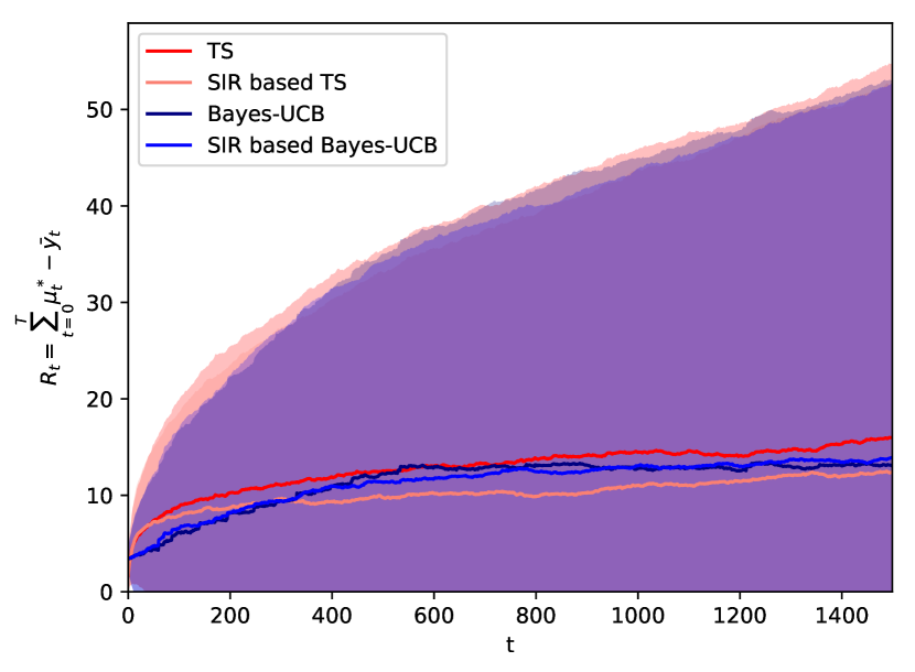
(f) Contextual Gaussian bandit,
$\theta_{0}=(-1,-1),\theta_{1}=(1,1),\sigma^{2}=1.0$.

Figure 13: Mean regret (standard deviation shown as shaded region) in static two-armed contextual Gaussian bandits with reward variance.

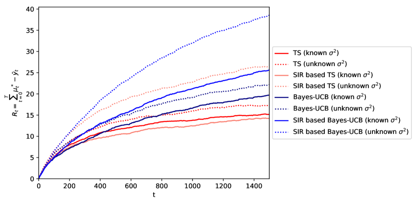
(a) Contextual Gaussian bandit,
$\theta_{0}=(-0.1,-0.1),\theta_{1}=(0.1,0.1),\sigma^{2}=0.5$.

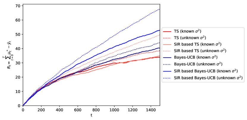
(b) Contextual Gaussian bandit,
$\theta_{0}=(-0.1,-0.1),\theta_{1}=(0.1,0.1),\sigma^{2}=1.0$.

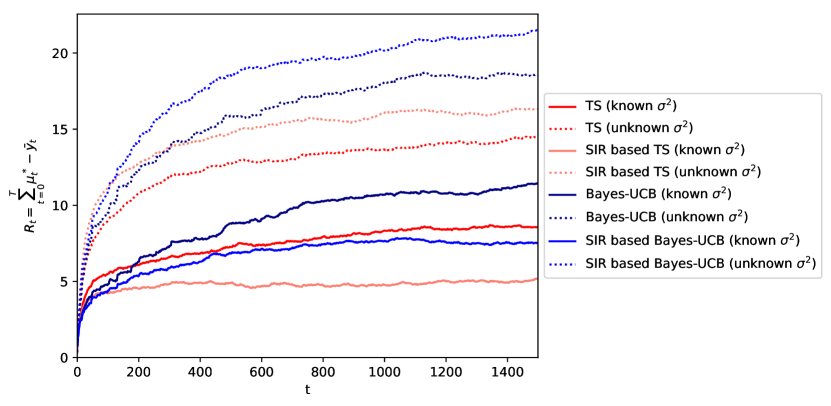
(c) Contextual Gaussian bandit,
$\theta_{0}=(-0.5,-0.5),\theta_{1}=(0.5,0.5),\sigma^{2}=0.5$.

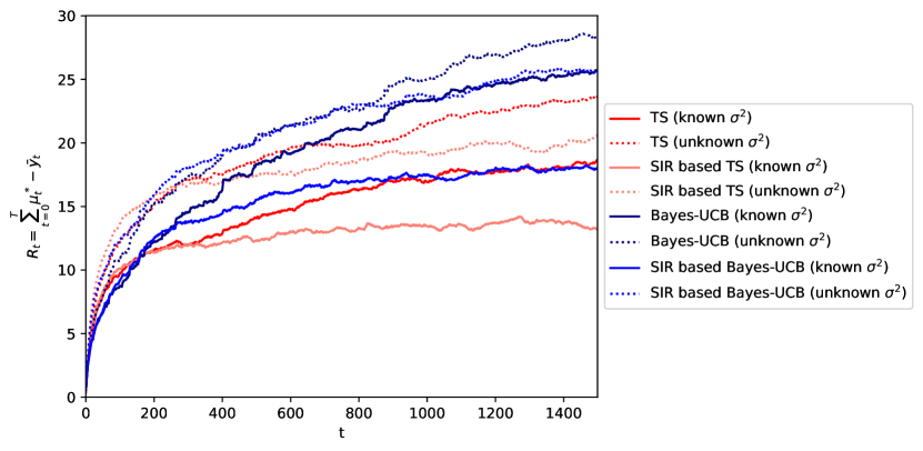
(d) Contextual Gaussian bandit,
$\theta_{0}=(-0.5,-0.5),\theta_{1}=(0.5,0.5),\sigma^{2}=1.0$.

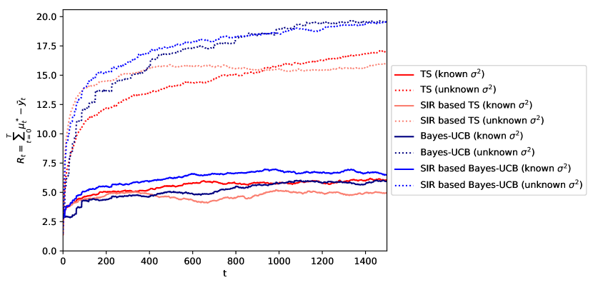
(e) Contextual Gaussian bandit,
$\theta_{0}=(-1,-1),\theta_{1}=(1,1),\sigma^{2}=0.5$.

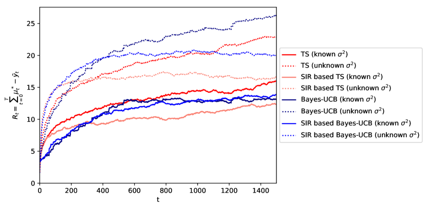
(f) Contextual Gaussian bandit,
$\theta_{0}=(-1,-1),\theta_{1}=(1,1),\sigma^{2}=1.0$.

Figure 14: Mean regret (standard deviation shown as shaded region) in static two-armed contextual Gaussian bandits with unknown reward variance.

B.1.5 Contextual Linear Gaussian bandits, A=3

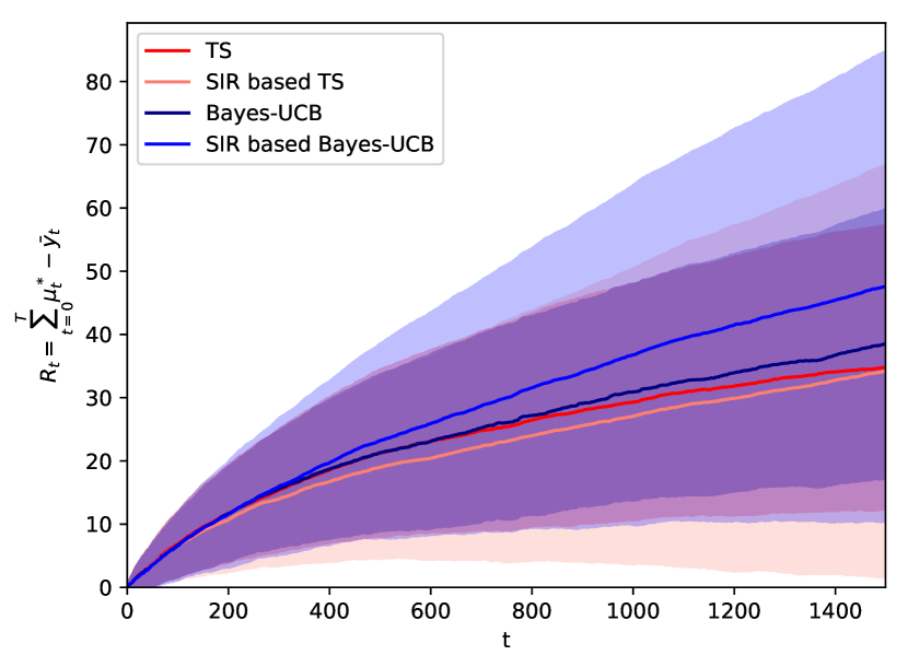
(a) Contextual Gaussian bandit,
$\theta_{0}=(-0.1,-0.1),\theta_{1}=(0,0),\theta_{2}=(0.1,0.1),\sigma^{2}=0.5$.

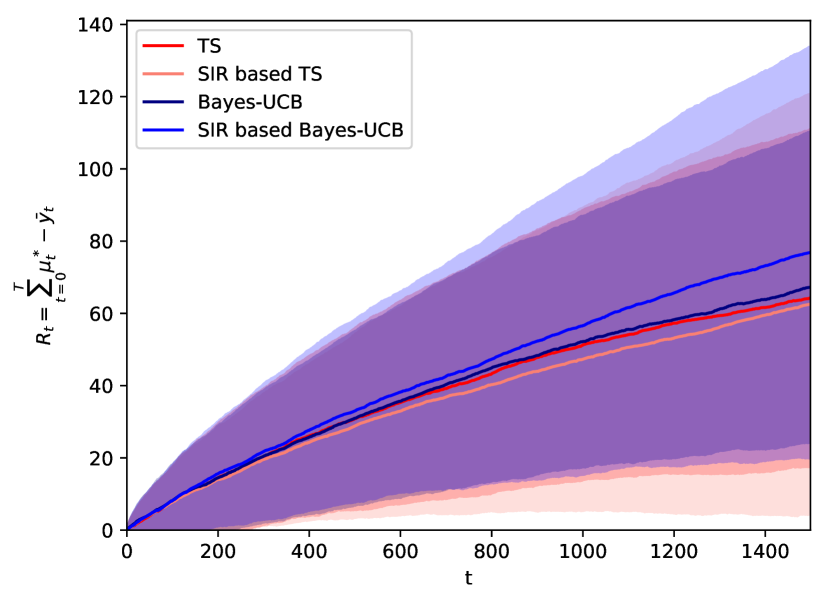
(b) Contextual Gaussian bandit,
$\theta_{0}=(-0.1,-0.1),\theta_{1}=(0,0),\theta_{2}=(0.1,0.1),\sigma^{2}=1.0$.

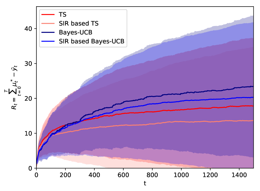
(c) Contextual Gaussian bandit,
$\theta_{0}=(-0.5,-0.5),\theta_{1}=(0,0),\theta_{2}=(0.5,0.5),\sigma^{2}=0.5$.

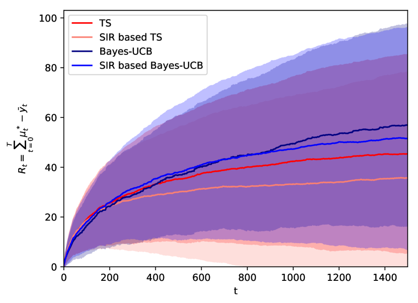
(d) Contextual Gaussian bandit,
$\theta_{0}=(-0.5,-0.5),\theta_{1}=(0,0),\theta_{2}=(0.5,0.5),\sigma^{2}=1.0$.

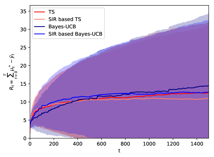
(e) Contextual Gaussian bandit,
$\theta_{0}=(-1,-1),\theta_{1}=(0,0),\theta_{2}=(1,1),\sigma^{2}=0.5$.

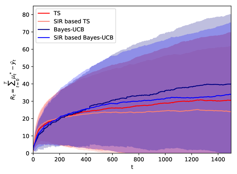
(f) Contextual Gaussian bandit,
$\theta_{0}=(-1,-1),\theta_{1}=(0,0),\theta_{2}=(1,1),\sigma^{2}=1.0$.

Figure 15: Mean regret (standard deviation shown as shaded region) in static three-armed contextual Gaussian bandits with reward variance.

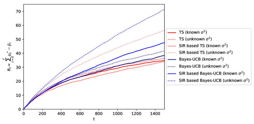
(a) Contextual Gaussian bandit,
$\theta_{0}=(-0.1,-0.1),\theta_{1}=(0,0),\theta_{2}=(0.1,0.1),\sigma^{2}=0.5$.

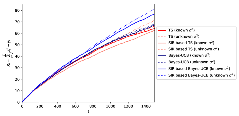
(b) Contextual Gaussian bandit,
$\theta_{0}=(-0.1,-0.1),\theta_{1}=(0,0),\theta_{2}=(0.1,0.1),\sigma^{2}=1.0$.

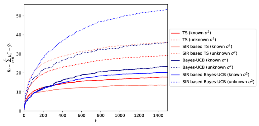
(c) Contextual Gaussian bandit,
$\theta_{0}=(-0.5,-0.5),\theta_{1}=(0,0),\theta_{2}=(0.5,0.5),\sigma^{2}=0.5$.

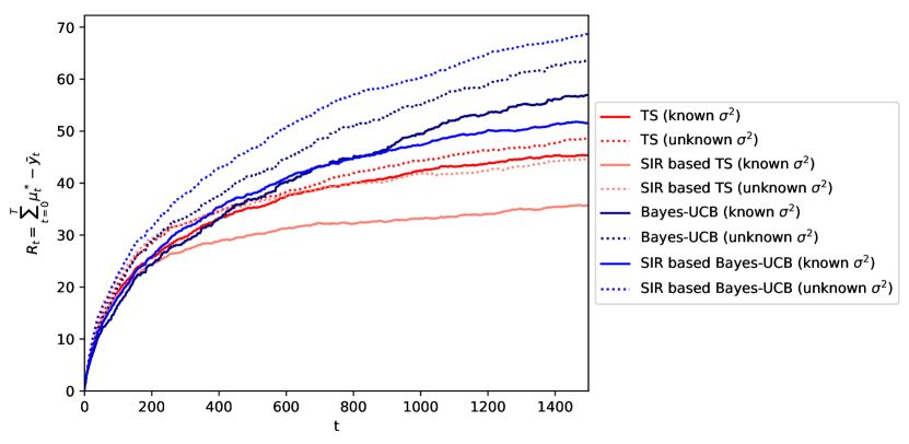
(d) Contextual Gaussian bandit,
$\theta_{0}=(-0.5,-0.5),\theta_{1}=(0,0),\theta_{2}=(0.5,0.5),\sigma^{2}=1.0$.

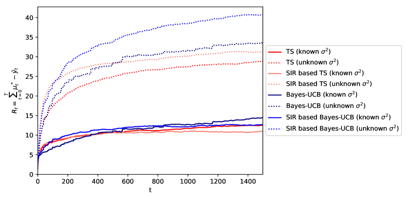
(e) Contextual Gaussian bandit,
$\theta_{0}=(-1,-1),\theta_{1}=(0,0),\theta_{2}=(1,1),\sigma^{2}=0.5$.

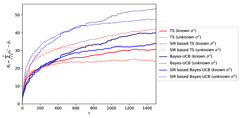
(f) Contextual Gaussian bandit,
$\theta_{0}=(-1,-1),\theta_{1}=(0,0),\theta_{2}=(1,1),\sigma^{2}=1.0$.

Figure 16: Mean regret (standard deviation shown as shaded region) in static three-armed contextual Gaussian bandits with unknown reward variance.

B.1.6 Contextual Linear Gaussian bandits, A=5

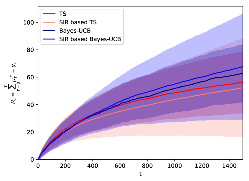
(a) Contextual Gaussian bandit,
$\theta_{0}=(-0.2,-0.2),\theta_{1}=(-0.1,-0.1),\theta_{2}=(0,0),\theta_{3}=(0.1,0.1),\theta_{4}=(0.2,0.2),\sigma^{2}=0.5$.

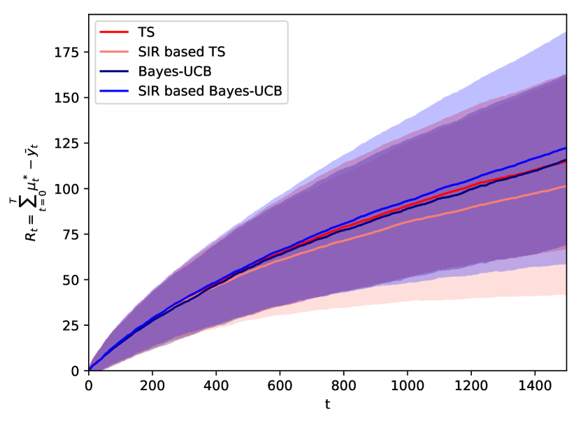
(b) Contextual Gaussian bandit,
$\theta_{0}=(-0.2,-0.2),\theta_{1}=(-0.1,-0.1),\theta_{2}=(0,0),\theta_{3}=(0.1,0.1),\theta_{4}=(0.2,0.2),\sigma^{2}=1.0$.

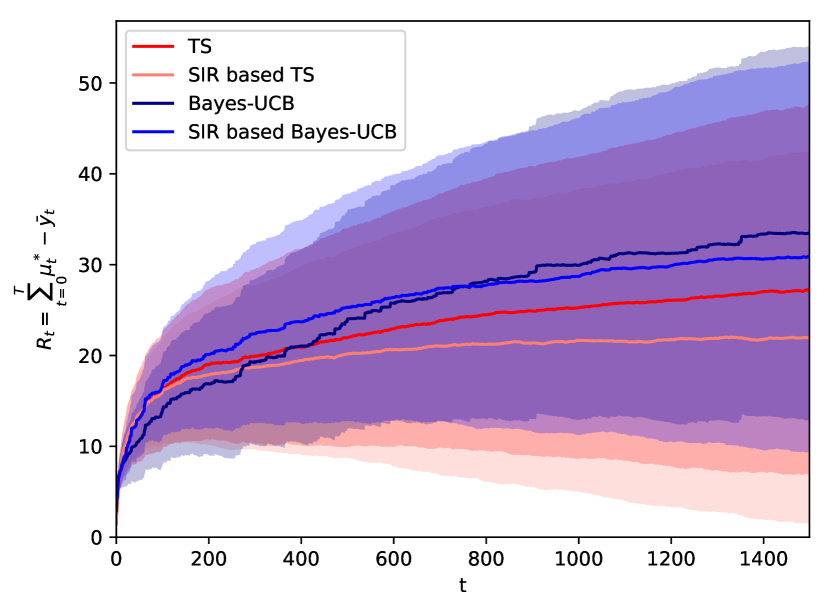
(c) Contextual Gaussian bandit,
$\theta_{0}=(-1.0,-1.0),\theta_{1}=(-0.5,-0.5),\theta_{2}=(0,0),\theta_{3}=(0.5,0.5),\theta_{4}=(1.0,1.0),\sigma^{2}=0.5$.

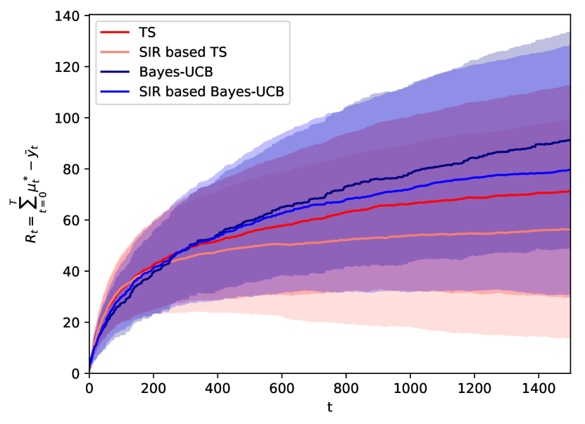
(d) Contextual Gaussian bandit,
$\theta_{0}=(-1.0,-1.0),\theta_{1}=(-0.5,-0.5),\theta_{2}=(0,0),\theta_{3}=(0.5,0.5),\theta_{4}=(1.0,1.0),\sigma^{2}=1.0$.

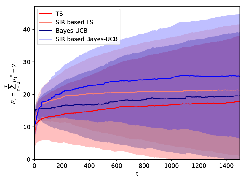
(e) Contextual Gaussian bandit,
$\theta_{0}=(-2,-2),\theta_{1}=(-1,-1),\theta_{2}=(0,0),\theta_{3}=(1,1),\theta_{4}=(2,2),\sigma^{2}=0.5$.

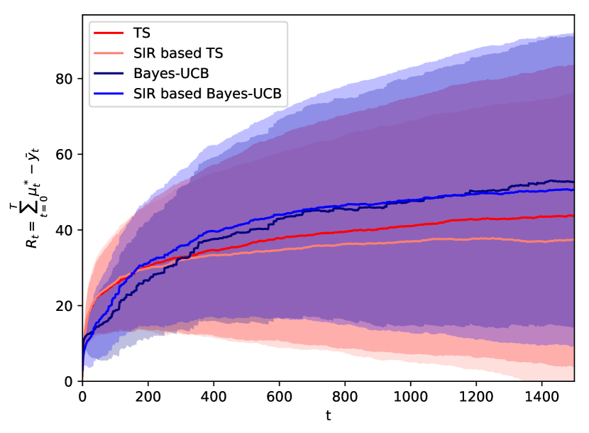
(f) Contextual Gaussian bandit,
$\theta_{0}=(-2,-2),\theta_{1}=(-1,-1),\theta_{2}=(0,0),\theta_{3}=(1,1),\theta_{4}=(2,2),\sigma^{2}=1.0$.

Figure 17: Mean regret (standard deviation shown as shaded region) in static five-armed contextual Gaussian bandits with reward variance.

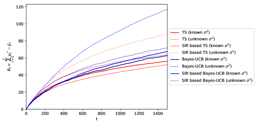
(a) Contextual Gaussian bandit,
$\theta_{0}=(-0.2,-0.2),\theta_{1}=(-0.1,-0.1),\theta_{2}=(0,0),\theta_{3}=(0.1,0.1),\theta_{4}=(0.2,0.2),\sigma^{2}=0.5$.

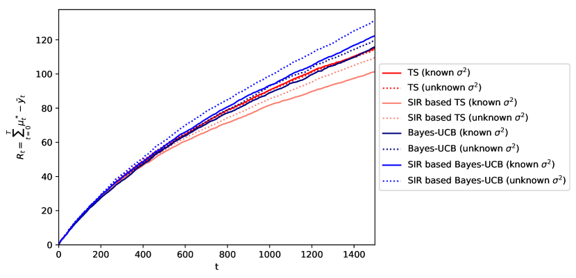
(b) Contextual Gaussian bandit,
$\theta_{0}=(-0.2,-0.2),\theta_{1}=(-0.1,-0.1),\theta_{2}=(0,0),\theta_{3}=(0.1,0.1),\theta_{4}=(0.2,0.2),\sigma^{2}=1.0$.

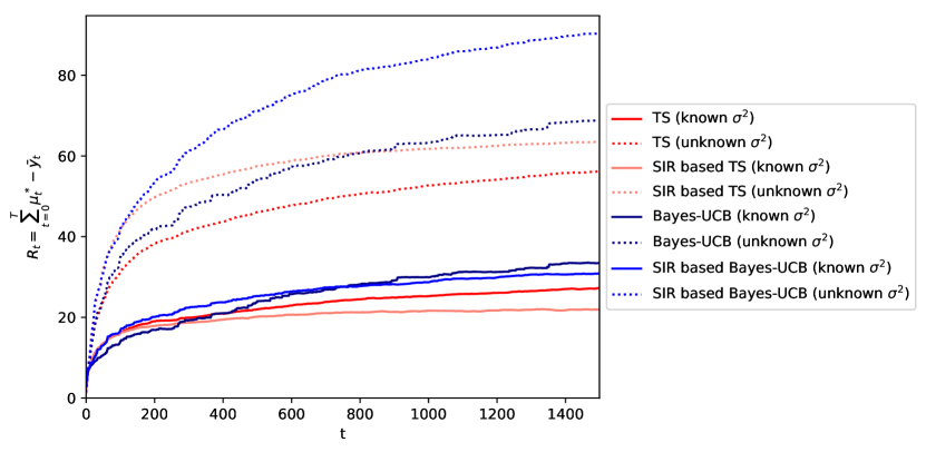
(c) Contextual Gaussian bandit,
$\theta_{0}=(-1.0,-1.0),\theta_{1}=(-0.5,-0.5),\theta_{2}=(0,0),\theta_{3}=(0.5,0.5),\theta_{4}=(1.0,1.0),\sigma^{2}=0.5$.

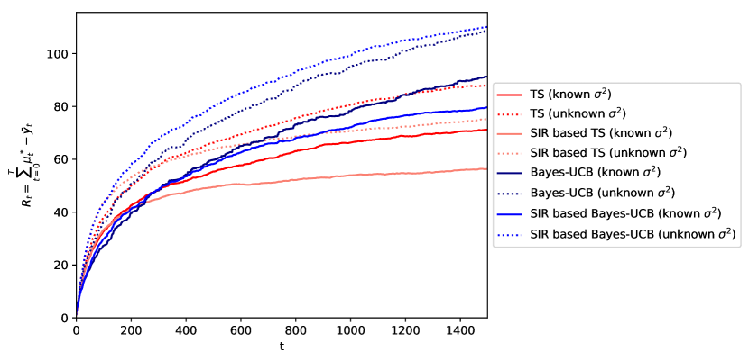
(d) Contextual Gaussian bandit,
$\theta_{0}=(-1.0,-1.0),\theta_{1}=(-0.5,-0.5),\theta_{2}=(0,0),\theta_{3}=(0.5,0.5),\theta_{4}=(1.0,1.0),\sigma^{2}=1.0$.

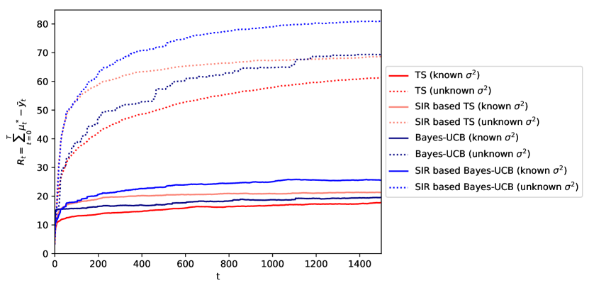
(e) Contextual Gaussian bandit,
$\theta_{0}=(-2,-2),\theta_{1}=(-1,-1),\theta_{2}=(0,0),\theta_{3}=(1,1),\theta_{4}=(2,2),\sigma^{2}=0.5$.

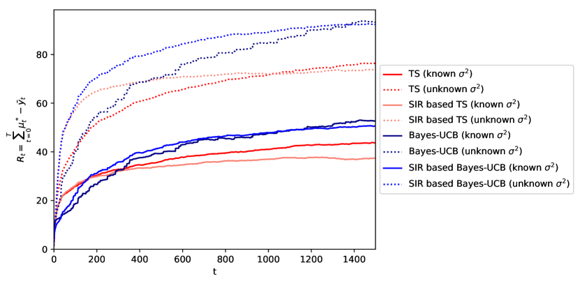
(f) Contextual Gaussian bandit,
$\theta_{0}=(-2,-2),\theta_{1}=(-1,-1),\theta_{2}=(0,0),\theta_{3}=(1,1),\theta_{4}=(2,2),\sigma^{2}=1.0$.

Figure 18: Mean regret (standard deviation shown as shaded region) in static five-armed contextual Gaussian bandits with unknown reward variance.

B.1.7 Contextual Logistic bandits, A=2

(a) Contextual Logistic bandit,
$\theta_{0}=(-0.1,-0.1),\theta_{1}=(0.1,0.1)$.

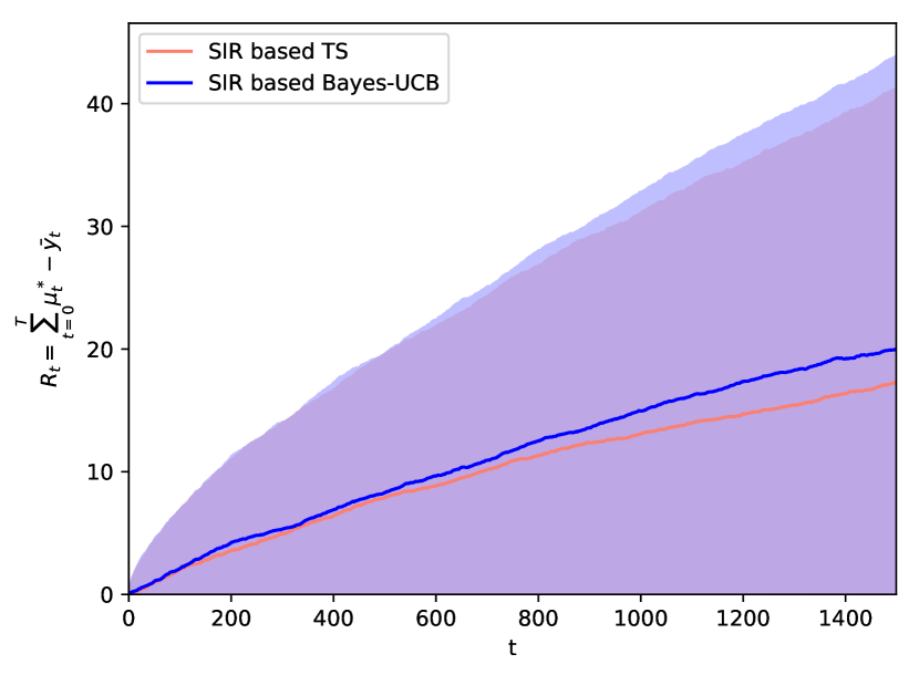
(b) Contextual Logistic bandit,
$\theta_{0}=(-0.1,-0.1),\theta_{1}=(0.1,0.1)$.

(c) Contextual Logistic bandit,
$\theta_{0}=(-0.5,-0.5),\theta_{1}=(0.5,0.5)$.

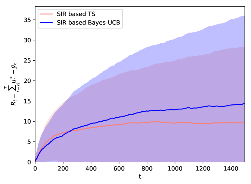
(d) Contextual Logistic bandit,
$\theta_{0}=(-0.5,-0.5),\theta_{1}=(0.5,0.5)$.

(e) Contextual Logistic bandit,
$\theta_{0}=(-1,-1),\theta_{1}=(1,1)$.

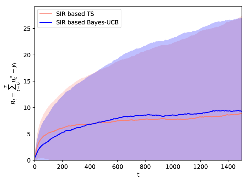
(f) Contextual Logistic bandit,
$\theta_{0}=(-1,-1),\theta_{1}=(1,1)$.

Figure 19: Mean regret (standard deviation shown as shaded region) in static two-armed contextual Logistic bandits.

B.1.8 Contextual Logistic bandits, A=3

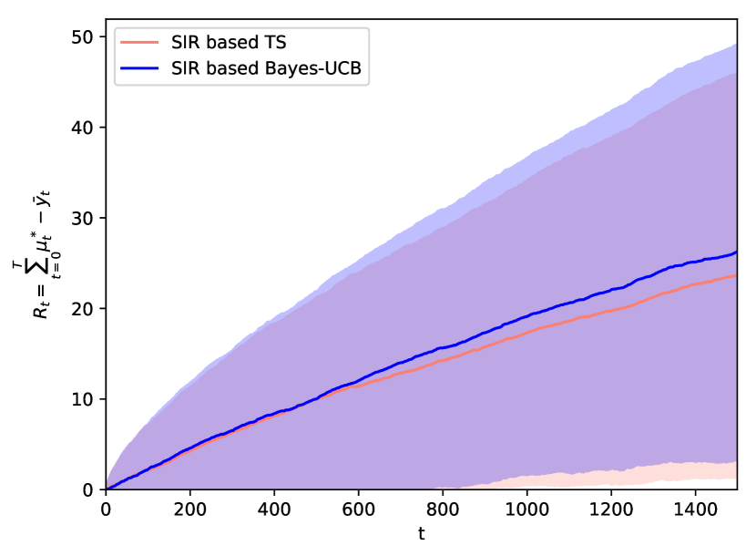
(a) Contextual Logistic bandit,
$\theta_{0}=(-0.1,-0.1),\theta_{1}=(0,0),\theta_{2}=(0.1,0.1)$.

(b) Contextual Logistic bandit,
$\theta_{0}=(-0.1,-0.1),\theta_{1}=(0,0),\theta_{2}=(0.1,0.1)$.

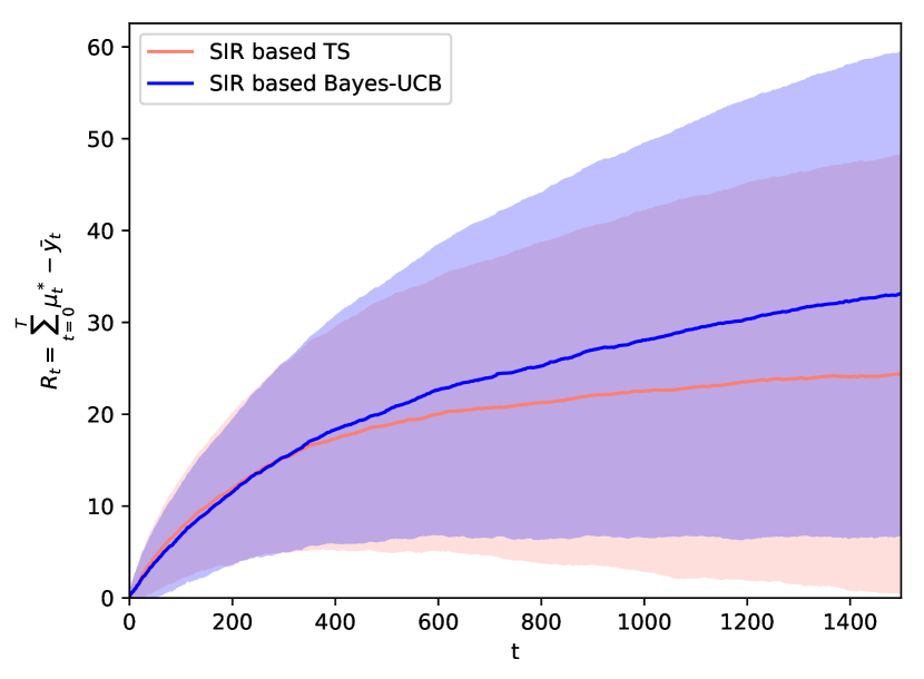
(c) Contextual Logistic bandit,
$\theta_{0}=(-0.5,-0.5),\theta_{1}=(0,0),\theta_{2}=(0.5,0.5)$.

(d) Contextual Logistic bandit,
$\theta_{0}=(-0.5,-0.5),\theta_{1}=(0,0),\theta_{2}=(0.5,0.5)$.

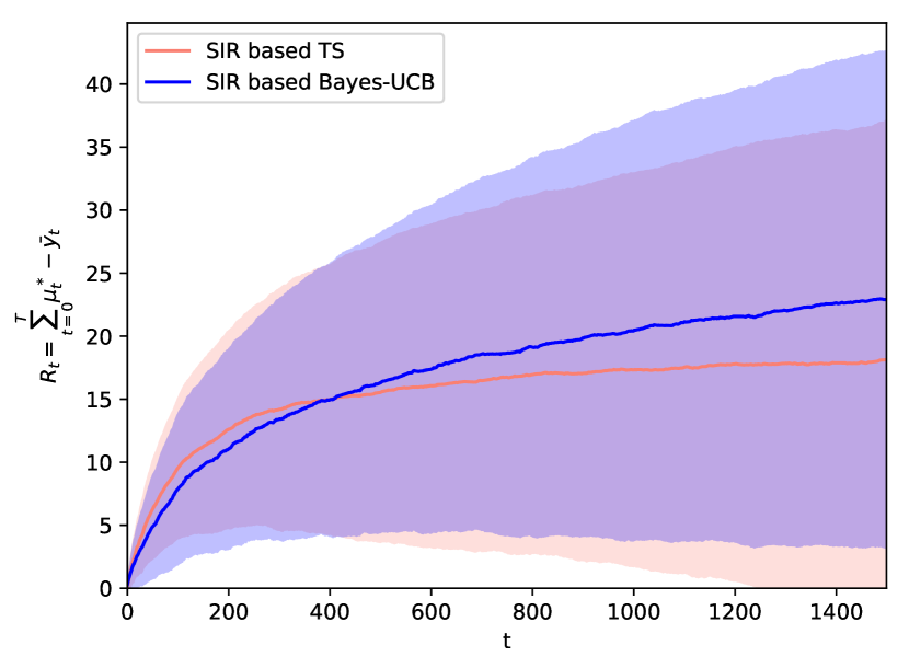
(e) Contextual Logistic bandit,
$\theta_{0}=(-1,-1),\theta_{1}=(0,0),\theta_{2}=(1,1)$.

(f) Contextual Logistic bandit,
$\theta_{0}=(-1,-1),\theta_{1}=(0,0),\theta_{2}=(1,1)$.

Figure 20: Mean regret (standard deviation shown as shaded region) in static three-armed contextual Logistic bandits.

B.1.9 Contextual Logistic bandits, A=5

(a) Contextual Logistic bandit,
$\theta_{0}=(-0.2,-0.2),\theta_{1}=(-0.1,-0.1),\theta_{2}=(0,0),\theta_{3}=(0.1,0.1),\theta_{4}=(0.2,0.2)$.

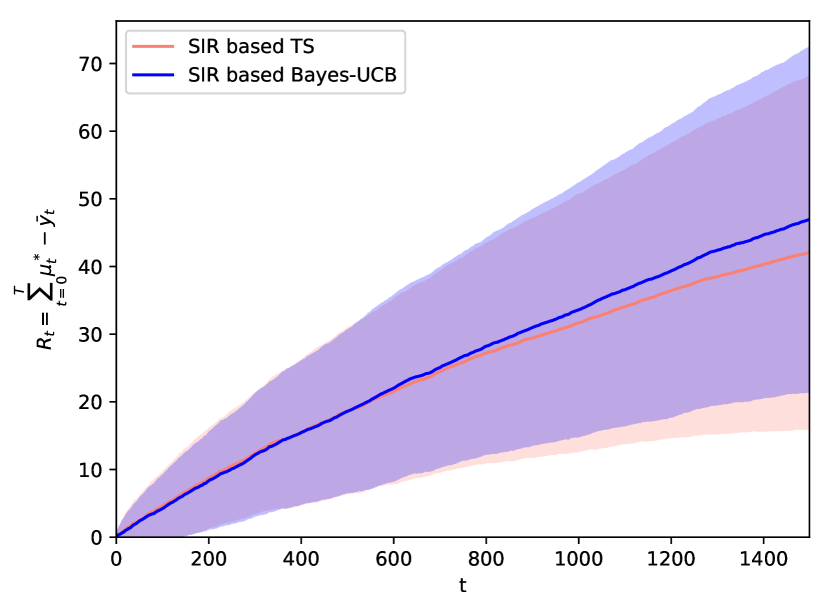
(b) Contextual Logistic bandit,
$\theta_{0}=(-0.2,-0.2),\theta_{1}=(-0.1,-0.1),\theta_{2}=(0,0),\theta_{3}=(0.1,0.1),\theta_{4}=(0.2,0.2)$.

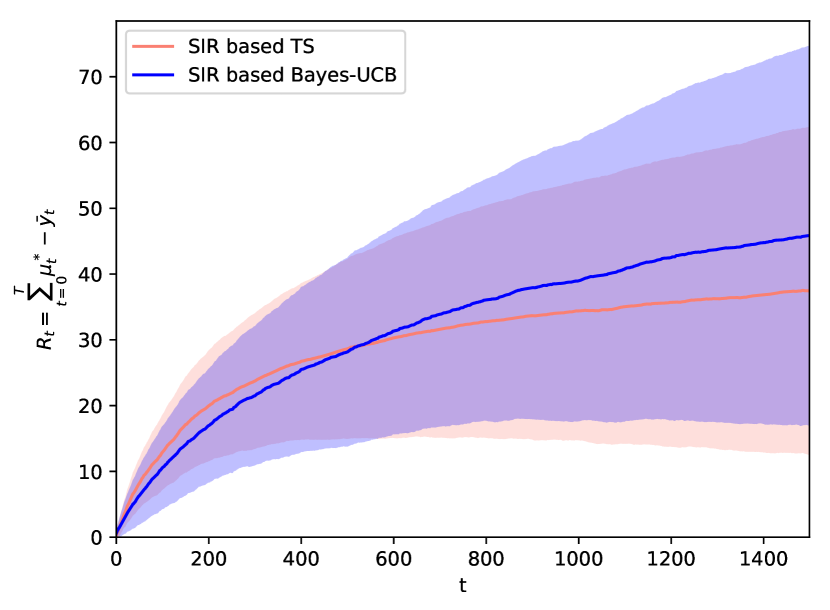
(c) Contextual Logistic bandit,
$\theta_{0}=(-1.0,-1.0),\theta_{1}=(-0.5,-0.5),\theta_{2}=(0,0),\theta_{3}=(0.5,0.5),\theta_{4}=(1.0,1.0)$.

(d) Contextual Logistic bandit,
$\theta_{0}=(-1.0,-1.0),\theta_{1}=(-0.5,-0.5),\theta_{2}=(0,0),\theta_{3}=(0.5,0.5),\theta_{4}=(1.0,1.0)$.

(e) Contextual Logistic bandit,
$\theta_{0}=(-2,-2),\theta_{1}=(-1,-1),\theta_{2}=(0,0),\theta_{3}=(1,1),\theta_{4}=(2,2)$.

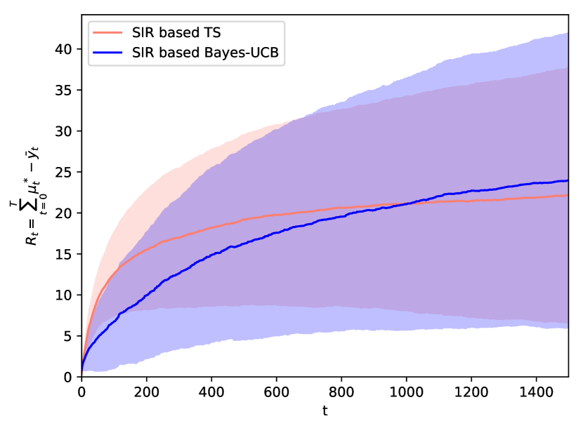
(f) Contextual Logistic bandit,
$\theta_{0}=(-2,-2),\theta_{1}=(-1,-1),\theta_{2}=(0,0),\theta_{3}=(1,1),\theta_{4}=(2,2)$.

Figure 21: Mean regret (standard deviation shown as shaded region) in static five-armed contextual Logistic bandits.

References

- Abbasi-Yadkori et al. (2011) Y. Abbasi-Yadkori, D. Pál, and C. Szepesvári. Improved Algorithms for Linear Stochastic Bandits. In J. Shawe-Taylor, R. S. Zemel, P. L. Bartlett, F. Pereira, and K. Q. Weinberger, editors, Advances in Neural Information Processing Systems 24, pages 2312–2320. Curran Associates, Inc., 2011. URL https://papers.nips.cc/paper/4417-improved-algorithms-for-linear-stochastic-bandits.
- Agarwal (2013) D. Agarwal. Computational Advertising: The Linkedin Way. In Proceedings of the 22Nd ACM International Conference on Information & Knowledge Management, CIKM ’13, pages 1585–1586, New York, NY, USA, 2013. ACM. ISBN 978-1-4503-2263-8. doi: 10.1145/2505515.2514690. URL http://doi.acm.org/10.1145/2505515.2514690.
- Agrawal and Goyal (2011) S. Agrawal and N. Goyal. Analysis of Thompson Sampling for the multi-armed bandit problem. CoRR, abs/1111.1797, 2011.
- Agrawal and Goyal (2012a) S. Agrawal and N. Goyal. Thompson Sampling for Contextual Bandits with Linear Payoffs. CoRR, abs/1209.3352, 2012a.
- Agrawal and Goyal (2012b) S. Agrawal and N. Goyal. Further Optimal Regret Bounds for Thompson Sampling. CoRR, abs/1209.3353, 2012b.
- Andrieu et al. (2010) C. Andrieu, A. Doucet, and R. Holenstein. Particle markov chain monte carlo methods. Journal of the Royal Statistical Society: Series B (Statistical Methodology), 72(3):269–342, 2010.
- Arulampalam et al. (2002) M. S. Arulampalam, S. Maskell, N. Gordon, and T. Clapp. A tutorial on particle filters for online nonlinear/non-Gaussian Bayesian tracking. Signal Processing, IEEE Transactions on, 50(2):174–188, 2 2002. ISSN 1053-587X.
- Auer et al. (2002) P. Auer, N. Cesa-Bianchi, and P. Fischer. Finite-time Analysis of the Multiarmed Bandit Problem. Machine Learning, 47(2-3):235–256, May 2002. ISSN 0885-6125. doi: 10.1023/A:1013689704352.
- Bai et al. (2013) A. Bai, F. Wu, and X. Chen. Bayesian Mixture Modelling and Inference based Thompson Sampling in Monte-Carlo Tree Search. In C. J. C. Burges, L. Bottou, M. Welling, Z. Ghahramani, and K. Q. Weinberger, editors, Advances in Neural Information Processing Systems 26, pages 1646–1654. Curran Associates, Inc., 2013. URL http://papers.nips.cc/paper/5111-bayesian-mixture-modelling-and-inference-based-thompson-sampling-in-monte-carlo-tree-search.pdf.
- Bernardo and Smith (2009) J. M. Bernardo and A. F. Smith. Bayesian Theory. Wiley Series in Probability and Statistics. Wiley, 2009. ISBN 9780470317716. doi: 10.1002/9780470316870.
- Besbes et al. (2014) O. Besbes, Y. Gur, and A. Zeevi. Stochastic multi-armed-bandit problem with non-stationary rewards. In Z. Ghahramani, M. Welling, C. Cortes, N. D. Lawrence, and K. Q. Weinberger, editors, Advances in Neural Information Processing Systems 27, pages 199–207. Curran Associates, Inc., 2014. URL http://papers.nips.cc/paper/5378-stochastic-multi-armed-bandit-problem-with-non-stationary-rewards.
- Bishop (2006) C. Bishop. Pattern Recognition and Machine Learning. Information Science and Statistics. Springer-Verlag New York, 2006.
- Blundell et al. (2015) C. Blundell, J. Cornebise, K. Kavukcuoglu, and D. Wierstra. Weight Uncertainty in Neural Networks. In Proceedings of the 32Nd International Conference on International Conference on Machine Learning - Volume 37, ICML’15, pages 1613–1622. JMLR.org, 2015.
- Box and Jenkins (1976) G. Box and G. Jenkins. Time Series Analysis: Forecasting and Control. Holden-Day series in time series analysis and digital processing. Holden-Day, 1976. ISBN 9780816211043. URL http://books.google.es/books?id=1WVHAAAAMAAJ.
- Brezzi and Lai (2002) M. Brezzi and T. L. Lai. Optimal learning and experimentation in bandit problems. Journal of Economic Dynamics and Control, 27(1):87 – 108, 2002. ISSN 0165-1889. doi: https://doi.org/10.1016/S0165-1889(01)00028-8.
- Brockwell and Davis (1991) P. J. Brockwell and R. A. Davis. Time Series: Theory and Methods. Springer Series in Statistics. Springer, 2nd edition, 1991. ISBN 1441903194,9781441903198. URL http://gen.lib.rus.ec/book/index.php?md5=A7050C98E54F74341373675D192A22FE.
- Carvalho et al. (2010) C. M. Carvalho, M. S. Johannes, H. F. Lopes, and N. G. Polson. Particle Learning and Smoothing. Statist. Sci., 25(1):88–106, 02 2010.
- Chapelle and Li (2011) O. Chapelle and L. Li. An Empirical Evaluation of Thompson Sampling. In J. Shawe-Taylor, R. S. Zemel, P. L. Bartlett, F. Pereira, and K. Q. Weinberger, editors, Advances in Neural Information Processing Systems 24, pages 2249–2257. Curran Associates, Inc., 2011. URL https://papers.nips.cc/paper/4321-an-empirical-evaluation-of-thompson-sampling.
- Cherkassky and Bornn (2013) M. Cherkassky and L. Bornn. Sequential Monte Carlo Bandits. ArXiv e-prints, Oct. 2013.
- Chopin (2004) N. Chopin. Central Limit Theorem for Sequential Monte Carlo Methods and Its Application to Bayesian Inference. The Annals of Statistics, 32(6):2385–2411, 2004. ISSN 00905364.
- Chopin et al. (2011) N. Chopin, P. E. Jacob, and O. Papaspiliopoulos. SMC2̂: an efficient algorithm for sequential analysis of state-space models. ArXiv e-prints, Jan. 2011.
- Chu et al. (2009) W. Chu, S.-T. Park, T. Beaupre, N. Motgi, A. Phadke, S. Chakraborty, and J. Zachariah. A Case Study of Behavior-driven Conjoint Analysis on Yahoo!: Front Page Today Module. In Proceedings of the 15th ACM SIGKDD International Conference on Knowledge Discovery and Data Mining, KDD ’09, pages 1097–1104, New York, NY, USA, 2009. ACM. ISBN 978-1-60558-495-9. doi: 10.1145/1557019.1557138.
- Creal (2012) D. Creal. A Survey of Sequential Monte Carlo Methods for Economics and Finance. Econometric Reviews, 31(3):245–296, 2012.
- Crisan and Doucet (2002) D. Crisan and A. Doucet. A survey of convergence results on particle filtering methods for practitioners. IEEE Transactions on Signal Processing, 50(3):736–746, Mar 2002. ISSN 1053-587X. doi: 10.1109/78.984773.
- Crisan and Míguez (2013) D. Crisan and J. Míguez. Nested particle filters for online parameter estimation in discrete-time state-space Markov models. ArXiv e-prints, Aug 2013.
- Djurić and Bugallo (2010) P. M. Djurić and M. F. Bugallo. Particle Filtering, chapter 5, pages 271–331. Wiley-Blackwell, 2010. ISBN 9780470575758. doi: 10.1002/9780470575758.ch5.
- Djurić et al. (2003) P. M. Djurić, J. H. Kotecha, J. Zhang, Y. Huang, T. Ghirmai, M. F. Bugallo, and J. Míguez. Particle Filtering. IEEE Signal Processing Magazine, 20(5):19–38, 9 2003.
- Djurić et al. (2004) P. M. Djurić, M. F. Bugallo, and J. Míguez. Density assisted particle filters for state and parameter estimation. In 2004 IEEE International Conference on Acoustics, Speech, and Signal Processing, (ICASSP), volume 2, pages ii – 701–704, 5 2004. doi: 10.1109/ICASSP.2004.1326354.
- Doucet et al. (2000) A. Doucet, N. de Freitas, K. P. Murphy, and S. J. Russell. Rao-Blackwellised Particle Filtering for Dynamic Bayesian Networks. In Proceedings of the 16th Conference on Uncertainty in Artificial Intelligence, UAI ’00, pages 176–183, San Francisco, CA, USA, 2000. Morgan Kaufmann Publishers Inc. ISBN 1-55860-709-9.
- Doucet et al. (2001) A. Doucet, N. D. Freitas, and N. Gordon, editors. Sequential Monte Carlo Methods in Practice. Springer, 2001.
- Dumitrascu et al. (2018) B. Dumitrascu, K. Feng, and B. Engelhardt. PG-TS: Improved Thompson Sampling for Logistic Contextual Bandits. In S. Bengio, H. Wallach, H. Larochelle, K. Grauman, N. Cesa-Bianchi, and R. Garnett, editors, Advances in Neural Information Processing Systems 31, pages 4629–4638. Curran Associates, Inc., 2018. URL http://papers.nips.cc/paper/7713-pg-ts-improved-thompson-sampling-for-logistic-contextual-bandits.pdf.
- Durbin and Koopman (2001) J. Durbin and S. J. Koopman. Time Series Analysis by State-Space Methods. Oxford Statistical Science Series. Oxford University Press, 2001.
- Durbin and Koopman (2012) J. Durbin and S. J. Koopman. Time Series Analysis by State-Space Methods: Second Edition. Oxford Statistical Science Series. Oxford University Press, 2 edition, 2012. ISBN 9780199641178. URL https://books.google.es/books?id=fOq39Zh0olQC.
- Eckles and Kaptein (2019) D. Eckles and M. Kaptein. Bootstrap Thompson Sampling and Sequential Decision Problems in the Behavioral Sciences. SAGE Open, 9(2):2158244019851675, 2019. doi: 10.1177/2158244019851675. URL https://doi.org/10.1177/2158244019851675.
- Ferreira et al. (2018) K. J. Ferreira, D. Simchi-Levi, and H. Wang. Online Network Revenue Management Using Thompson Sampling. Operations Research, 66(6):1586–1602, 2018. doi: 10.1287/opre.2018.1755. URL https://doi.org/10.1287/opre.2018.1755.
- Garivier and Cappé (2011) A. Garivier and O. Cappé. The KL-UCB Algorithm for Bounded Stochastic Bandits and Beyond. In S. M. Kakade and U. von Luxburg, editors, Proceedings of the 24th Annual Conference on Learning Theory, volume 19 of Proceedings of Machine Learning Research, pages 359–376, Budapest, Hungary, 09–11 Jun 2011. PMLR. URL http://proceedings.mlr.press/v19/garivier11a.html.
- Garivier and Moulines (2011) A. Garivier and E. Moulines. On upper-confidence bound policies for switching bandit problems. In Proceedings of the 22Nd International Conference on Algorithmic Learning Theory, ALT’11, pages 174–188, Berlin, Heidelberg, 2011. Springer-Verlag. ISBN 978-3-642-24411-7. URL http://dl.acm.org/citation.cfm?id=2050345.2050365.
- Gittins (1979) J. C. Gittins. Bandit Processes and Dynamic Allocation Indices. Journal of the Royal Statistical Society. Series B (Methodological), 41(2):148–177, 1979. ISSN 00359246.
- Gopalan et al. (2014) A. Gopalan, S. Mannor, and Y. Mansour. Thompson Sampling for Complex Online Problems. In E. P. Xing and T. Jebara, editors, Proceedings of the 31st International Conference on Machine Learning, volume 32 of Proceedings of Machine Learning Research, pages 100–108, Bejing, China, 22–24 Jun 2014. PMLR. URL http://proceedings.mlr.press/v32/gopalan14.html.
- Gordon et al. (1993) N. J. Gordon, D. Salmond, and A. Smith. Novel approach to nonlinear/non-Gaussian Bayesian state estimation. Radar and Signal Processing, IEEE Proceedings, 140(2):107 –113, 4 1993. ISSN 0956-375X.
- Hill et al. (2017) D. N. Hill, H. Nassif, Y. Liu, A. Iyer, and S. Vishwanathan. An efficient bandit algorithm for realtime multivariate optimization. In Proceedings of the 23rd ACM SIGKDD International Conference on Knowledge Discovery and Data Mining, pages 1813–1821. ACM, 2017.
- Ionides et al. (2006) E. L. Ionides, C. Bretó, and A. A. King. Inference for nonlinear dynamical systems. Proceedings of the National Academy of Sciences, 103(49):18438–18443, 2006.
- Kalman (1960) R. E. Kalman. A New Approach to Linear Filtering and Prediction Problems. Transactions of the ASME–Journal of Basic Engineering, 82(Series D):35–45, 1960.
- Kandasamy et al. (2018) K. Kandasamy, A. Krishnamurthy, J. Schneider, and B. Poczos. Parallelised Bayesian Optimisation via Thompson Sampling. In A. Storkey and F. Perez-Cruz, editors, Proceedings of the Twenty-First International Conference on Artificial Intelligence and Statistics, volume 84 of Proceedings of Machine Learning Research, pages 133–142, Playa Blanca, Lanzarote, Canary Islands, 09–11 Apr 2018. PMLR. URL http://proceedings.mlr.press/v84/kandasamy18a.html.
- Kantas et al. (2015) N. Kantas, A. Doucet, S. S. Singh, J. Maciejowski, and N. Chopin. On particle methods for parameter estimation in state-space models. Statistical science, 30(3):328–351, 2015.
- Kaufmann et al. (2012) E. Kaufmann, O. Cappe, and A. Garivier. On Bayesian Upper Confidence Bounds for Bandit Problems. In N. D. Lawrence and M. Girolami, editors, Proceedings of the Fifteenth International Conference on Artificial Intelligence and Statistics, volume 22 of Proceedings of Machine Learning Research, pages 592–600, La Palma, Canary Islands, 21–23 Apr 2012. PMLR.
- Kawale et al. (2015) J. Kawale, H. H. Bui, B. Kveton, L. Tran-Thanh, and S. Chawla. Efficient Thompson Sampling for Online Matrix-Factorization Recommendation. In C. Cortes, N. D. Lawrence, D. D. Lee, M. Sugiyama, and R. Garnett, editors, Advances in Neural Information Processing Systems 28, pages 1297–1305. Curran Associates, Inc., 2015. URL http://papers.nips.cc/paper/5985-efficient-thompson-sampling-for-online-matrix-factorization-recommendation.pdf.
- Kingma et al. (2015) D. P. Kingma, T. Salimans, and M. Welling. Variational Dropout and the Local Reparameterization Trick. In C. Cortes, N. D. Lawrence, D. D. Lee, M. Sugiyama, and R. Garnett, editors, Advances in Neural Information Processing Systems 28, pages 2575–2583. Curran Associates, Inc., 2015.
- Korda et al. (2013) N. Korda, E. Kaufmann, and R. Munos. Thompson Sampling for 1-Dimensional Exponential Family Bandits. In C. J. C. Burges, L. Bottou, M. Welling, Z. Ghahramani, and K. Q. Weinberger, editors, Advances in Neural Information Processing Systems 26, pages 1448–1456. Curran Associates, Inc., 2013.
- Lai (1987) T. L. Lai. Adaptive Treatment Allocation and the Multi-Armed Bandit Problem. The Annals of Statistics, 15(3):1091–1114, 1987. ISSN 00905364.
- Lai and Robbins (1985) T. L. Lai and H. Robbins. Asymptotically Efficient Adaptive Allocation Rules. Advances in Applied Mathematics, 6(1):4–22, mar 1985. ISSN 0196-8858. doi: 10.1016/0196-8858(85)90002-8.
- Lamprier et al. (2017) S. Lamprier, T. Gisselbrecht, and P. Gallinari. Variational Thompson Sampling for Relational Recurrent Bandits. In M. Ceci, J. Hollmén, L. Todorovski, C. Vens, and S. Džeroski, editors, Machine Learning and Knowledge Discovery in Databases, pages 405–421, Cham, 2017. Springer International Publishing. ISBN 978-3-319-71246-8.
- Lattimore and Szepesvári (2019) T. Lattimore and C. Szepesvári. Bandit algorithms. Preprint, 2019.
- Li et al. (2016) C. Li, C. Chen, D. Carlson, and L. Carin. Preconditioned Stochastic Gradient Langevin Dynamics for Deep Neural Networks. In Proceedings of the Thirtieth AAAI Conference on Artificial Intelligence, AAAI’16, pages 1788–1794. AAAI Press, 2016.
- Li (2013) L. Li. Generalized Thompson Sampling for Contextual Bandits. ArXiv e-prints, Oct. 2013.
- Li et al. (2010) L. Li, W. Chu, J. Langford, and R. E. Schapire. A Contextual-Bandit Approach to Personalized News Article Recommendation. CoRR, abs/1003.0146, 2010.
- Li et al. (2015) T. Li, M. Bolić, and P. M. Djurić. Resampling Methods for Particle Filtering: Classification, implementation, and strategies. Signal Processing Magazine, IEEE, 32(3):70–86, 5 2015. ISSN 1053-5888.
- Lipton et al. (2016) Z. C. Lipton, X. Li, J. Gao, L. Li, F. Ahmed, and L. Deng. Efficient Dialogue Policy Learning with BBQ-Networks. ArXiv e-prints, Aug. 2016.
- Liu and West (2001) J. Liu and M. West. Combined Parameter and State Estimation in Simulation-Based Filtering, chapter 10, pages 197–223. Springer New York, New York, NY, 2001. ISBN 978-1-4757-3437-9. doi: 10.1007/978-1-4757-3437-9_10.
- Liu (2001) J. S. Liu. Monte Carlo Strategies in Scientific Computing. Springer Series in Statistics. Springer, 2001.
- Lu and Roy (2017) X. Lu and B. V. Roy. Ensemble Sampling. In I. Guyon, U. V. Luxburg, S. Bengio, H. Wallach, R. Fergus, S. Vishwanathan, and R. Garnett, editors, Advances in Neural Information Processing Systems 30, pages 3258–3266. Curran Associates, Inc., 2017. URL http://papers.nips.cc/paper/6918-ensemble-sampling.pdf.
- Martino et al. (2017) L. Martino, V. Elvira, and F. Louzada. Effective sample size for importance sampling based on discrepancy measures. Signal Processing, 131:386 – 401, 2017. ISSN 0165-1684.
- Mellor and Shapiro (2013) J. Mellor and J. Shapiro. Thompson Sampling in Switching Environments with Bayesian Online Change Detection. In C. M. Carvalho and P. Ravikumar, editors, Proceedings of the Sixteenth International Conference on Artificial Intelligence and Statistics, volume 31 of Proceedings of Machine Learning Research, pages 442–450, Scottsdale, Arizona, USA, 29 Apr–01 May 2013. PMLR. URL http://proceedings.mlr.press/v31/mellor13a.html.
- Merwe et al. (2001) R. V. D. Merwe, A. Doucet, N. D. Freitas, and E. A. Wan. The unscented particle filter. In Advances in neural information processing systems, pages 584–590, 2001.
- Netflix (2017) Netflix. Artwork Personalization at Netflix. medium.com, December 2017.
- Olsson and Westerborn (2014) J. Olsson and J. Westerborn. Efficient particle-based online smoothing in general hidden Markov models: the PaRIS algorithm. ArXiv e-prints, Dec 2014.
- Olsson et al. (2006) J. Olsson, O. Cappé, R. Douc, and E. Moulines. Sequential Monte Carlo smoothing with application to parameter estimation in non-linear state space models. ArXiv Mathematics e-prints, Sep 2006.
- Osband and Roy (2015) I. Osband and B. V. Roy. Bootstrapped Thompson sampling and deep exploration. arXiv preprint arXiv:1507.00300, 2015.
- Osband et al. (2016) I. Osband, C. Blundell, A. Pritzel, and B. V. Roy. Deep Exploration via Bootstrapped DQN. In D. D. Lee, M. Sugiyama, U. V. Luxburg, I. Guyon, and R. Garnett, editors, Advances in Neural Information Processing Systems 29, pages 4026–4034. Curran Associates, Inc., 2016.
- Raj and Kalyani (2017) V. Raj and S. Kalyani. Taming non-stationary bandits: A bayesian approach. arXiv preprint arXiv:1707.09727, 2017.
- Riquelme et al. (2018) C. Riquelme, G. Tucker, and J. Snoek. Deep Bayesian Bandits Showdown: An Empirical Comparison of Bayesian Deep Networks for Thompson Sampling. In International Conference on Learning Representations, 2018.
- Ristic et al. (2004) B. Ristic, S. Arulampalam, and N. Gordon. Beyond the Kalman Filter: Particle Filters for Tracking Applications. Artech House, 2004. ISBN 9781580538510.
- Robbins (1952) H. Robbins. Some aspects of the sequential design of experiments. Bulletin of the American Mathematical Society, (58):527–535, 1952.
- Russo and Roy (2014) D. Russo and B. V. Roy. Learning to optimize via posterior sampling. Mathematics of Operations Research, 39(4):1221–1243, 2014.
- Russo and Roy (2016) D. Russo and B. V. Roy. An information-theoretic analysis of Thompson sampling. The Journal of Machine Learning Research, 17(1):2442–2471, 2016.
- Russo et al. (2018) D. J. Russo, B. V. Roy, A. Kazerouni, I. Osband, and Z. Wen. A Tutorial on Thompson Sampling. Foundations and Trends® in Machine Learning, 11(1):1–96, 2018. ISSN 1935-8237. doi: 10.1561/2200000070. URL http://dx.doi.org/10.1561/2200000070.
- Schwartz et al. (2017) E. M. Schwartz, E. T. Bradlow, and P. S. Fader. Customer Acquisition via Display Advertising Using Multi-Armed Bandit Experiments. Marketing Science, 36(4):500–522, 2017. doi: 10.1287/mksc.2016.1023. URL https://doi.org/10.1287/mksc.2016.1023.
- Scott (2015) S. L. Scott. Multi-armed bandit experiments in the online service economy. Applied Stochastic Models in Business and Industry, 31:37–49, 2015. Special issue on actual impact and future perspectives on stochastic modelling in business and industry.
- Shumway and Stoffer (2010) R. H. Shumway and D. S. Stoffer. Time Series Analysis and Its Applications: With R Examples (Springer Texts in Statistics). Springer, 3rd edition, 2010. ISBN 144197864X,9781441978646. URL http://gen.lib.rus.ec/book/index.php?md5=9ef53da6af80708921f688661bce95e7.
- Sutton and Barto (1998) R. S. Sutton and A. G. Barto. Reinforcement Learning: An Introduction. MIT Press: Cambridge, MA, 1998.
- Thompson (1935) W. R. Thompson. On the Theory of Apportionment. American Journal of Mathematics, 57(2):450–456, 1935. ISSN 00029327, 10806377.
- Urteaga and Djurić (2016a) I. Urteaga and P. M. Djurić. Sequential Estimation of Hidden ARMA Processes by Particle Filtering - Part I. IEEE Transactions on Signal Processing, PP(99):1–1, 2016a. ISSN 1053-587X. doi: 10.1109/TSP.2016.2598309.
- Urteaga and Djurić (2016b) I. Urteaga and P. M. Djurić. Sequential Estimation of Hidden ARMA Processes by Particle Filtering - Part II. IEEE Transactions on Signal Processing, PP(99):1–1, 2016b. ISSN 1053-587X. doi: 10.1109/TSP.2016.2598324.
- Urteaga and Wiggins (2018) I. Urteaga and C. Wiggins. Variational inference for the multi-armed contextual bandit. In A. Storkey and F. Perez-Cruz, editors, Proceedings of the Twenty-First International Conference on Artificial Intelligence and Statistics, volume 84 of Proceedings of Machine Learning Research, pages 698–706, Playa Blanca, Lanzarote, Canary Islands, 09–11 Apr 2018. PMLR.
- Urteaga et al. (2017) I. Urteaga, M. F. Bugallo, and P. M. Djurić. Sequential Monte Carlo for inference of latent ARMA time-series with innovations correlated in time. EURASIP Journal on Advances in Signal Processing, 2017(1), Dec 2017. doi: 10.1186/s13634-017-0518-4. URL https://doi.org/10.1186/s13634-017-0518-4.
- van Leeuwen (2009) P. J. van Leeuwen. Particle Filtering in Geophysical Systems. Monthly Weather Review, 12(137):4089–4114., 2009.
- Whittle (1951) P. Whittle. Hypothesis Testing in Time Series Analysis. Almquist and Wicksell, 1951.