Luminosity constraint and entangled solar neutrino signals

Abstract

The current frontier of solar neutrino physics is the observation of CNO neutrinos. The signals of CNO and PP neutrinos are however entangled: In fact, the pp-flux can be known precisely only if CNO-flux is quantified; the interpretation of the gallium experiments depends upon both fluxes; a precise knowledge of pep-flux is a precondition to extract the CNO-neutrino signal with Borexino. The luminosity constraint plays an increasingly important rôle: we present it in a new form, improving the expression obtained by J. Bahcall.[1]

1 Introduction

The standard solar model (SSM) has always been a crucial tool to understand the Sun.[2] The expected solar neutrinos fluxes $\Phi_{i}$ are expressed as

$$\Phi_{i}=\varphi_{i}\times\frac{10^{\alpha_{i}}}{\mbox{cm${}^{2}$s}}\mbox{ where }{i=\mbox{\small pp,Be,pep,B,hep,N,O,F}}$$ (1)

Here, the index $i$ runs over the 5 neutrino fluxes of the PP-chain and the 3 neutrino fluxes of the CNO-cycle, $\alpha_{i}$ are fixed exponents and $\varphi_{i}$ adimensional coefficients. The SSM predictions of the last 30 years, including the recent ones overviewed by A. Serenelli,[3] are given in tab1. Note that,
1) the exponents $\alpha_{i}$ never changed, i.e., the orders of magnitude are stable;
2) the coefficients $\varphi_{i}$ of the CNO-cycle changed considerably.
The CNO-cycle is subdominant but also poorly known. In the most recent SSM, $\varphi_{\mbox{\tiny N}}$ goes from 3.20 (upper 1$\sigma$ range of GS98) to 1.75 (lower 1$\sigma$ range of AGSS09). The ensuing span $2.48\pm 0.73$ is compatible with $\varphi_{\mbox{\tiny N}}=0$ at 3.4$\sigma$, i.e., CNO-neutrinos could be absent at 0.06% CL. Thus,

a few $\sigma$ measurement will already impact on present knowledge.

Theoretical predictions for $\varphi_{i}$, i.e., for solar neutrino fluxes in 4 SSM. For non-symmetric BP2000 uncertainties, maximum errors are conservatively quoted. The PP-chain The CNO-cycle identification index $i$ pp Be pep B hep N O F exponent $\alpha_{i}$ 10 $9$ $8$ $6$ $3$ ${8}$ ${8}$ ${6}$ BU1988 [4] 6.0 4.7 1.4 5.8 7.6 6.1 5.2 5.2 errors 0.1 0.7 0.1 2.1 7.6 3.1 3.0 2.4 BP2000 [5] 5.95 4.77 1.40 5.05 9.3 5.48 4.80 5.63 errors 0.06 0.48 0.02 1.01 9.3 1.15 1.20 1.41 B16-GS98 [6] 5.98 4.93 1.44 5.46 7.98 2.78 2.05 5.29 errors 0.04 0.30 0.01 0.66 2.39 0.42 0.35 1.06 B16-AGSS09met [6] 6.03 4.50 1.46 4.50 8.25 2.04 1.44 3.26 errors 0.03 0.27 0.01 0.54 2.48 0.29 0.23 0.59

After the theory, we examine the data. Pioneer observatories Homestake, Kamiokande, Gallex/GNO and SAGE saw solar neutrinos as reviewed by K. Lande, T. Kirsten, V. Gavrin.[3] Their successors Super-Kamiokande and SNO measured precisely the B-neutrino flux, as discussed by Y. Suzuki and H. Robertson.[3] Borexino determined accurately the Be-neutrino component, studying B-neutrinos at the lowest energies and probing at $\sim$10% the pp- and pep-fluxes as reported by M. Wurm and D. Guffanti.[3] Borexino’s bound on the sum of CNO-neutrinos,

$$\color[rgb]{0,0,1}{\ \Phi_{\mbox{\tiny CNO}}\equiv\Phi_{\mbox{\tiny N}}+\Phi_{\mbox{\tiny N}}+\Phi_{\mbox{\tiny F}}\equiv\varphi_{\mbox{\tiny CNO}}\times\frac{10^{8}}{\mbox{cm${}^{2}$s}}}$$ (2)

is discussed later. To recap, 4 fluxes of the PP-chain out of 5 are known.

fig1 compares SSM predictions – in the version that agrees with helioseismology as discussed by F.L. Villante[3] – and energy thresholds of various experiments, i.e., the minimum energy that they can probe.[7] The experiments are grouped in 2 broad classes, i.e.,
$1^{\mbox{\tiny st}}$ :– the radiochemical experiments and the SNO-NC experiment. They ‘integrate’ above the energy threshold indicated by the arrows given in the upper border of fig1, or more precisely, they measure a suitable average of the fluxes–see K. Lande, T. Kirsten, V. Gavrin, H. Robertson;[3]
$2^{\mbox{\tiny nd}}$ :– the experiments based on elastic scattering on electrons $\nu+\mbox{e}\to\nu+\mbox{e}$ (ES) and the SNO-CC experiment. They probe the differential SSM fluxes in grey areas of fig1, i.e., they discriminate the individual fluxes–see Y. Suzuki, H. Robertson, M. Wurm and D. Guffanti.[3] Note that,

the experiments sensitive to CNO-neutrinos are only SAGE and Gallex/GNO, in the $1^{\mbox{\tiny st}}$ class, and Borexino, in the $2^{\mbox{\tiny nd}}$ one.

See[8] for more discussion. Note that ES cross section is very well known.

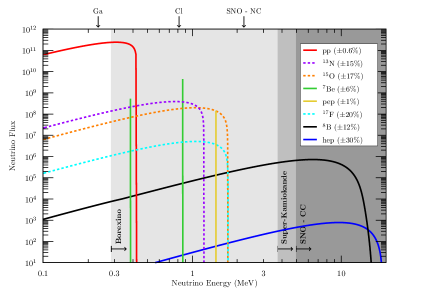
Figure 1: The 8 neutrino fluxes of the GS98 version of SSM, along with the sensitivity regions of the major present and past experiments.[7] The grey areas emphasize the regions of sensitivity of the few experiments that are able to probe the individual fluxes–see text for a discussion.

2 The luminosity constraint

In this section, we introduce and improve the description of the “luminosity constraint”, that connects the neutrino fluxes to the observed solar luminosity. The latter quantity–i.e., the power emitted in light/heat–is measured much better than the neutrino fluxes,[6] since the error is below percent,

$$L_{\mathrel{{{\odot}}}}^{\mbox{\tiny obs}}=3.8418\times 10^{33}\ \frac{\mbox{erg}}{\mbox{sec}},\mbox{ with }\frac{\delta L_{\mathrel{{{\odot}}}}^{\mbox{\tiny obs}}}{L_{\mathrel{{{\odot}}}}^{\mbox{\tiny obs}}}=0.4\;\%$$ (3)

By definition, this is included in the SSM, but the use of the luminosity constraint is a milder assumption than the use of the SSM itself; indeed, solar neutrino data-analyses that implement it are called model independent.

2.1 Physical derivation of the luminosity constraint

In the rudimentary model of J. Perrin,[9] 4 hydrogen atoms transform into 1 helium atom, releasing energy inside the Sun. Symbolically,

$$4\mbox{H}\to{}^{4}\mbox{He}+\mathcal{E}_{\mathrel{{{\odot}}}}$$ (4)

The energy released, i.e., the difference between the masses of the initial and final atomic species (first measured by F.W. Aston) is accurately known,

$$\mathcal{E}_{\mathrel{{{\odot}}}}=4M_{1}-M_{4}\approx 26.73097\mbox{ MeV}$$ (5)

we use $c=1$. Today we know that there are nuclear–not atomic–reactions in the Sun, but the estimation of the energy is almost unchanged. In fact, the effective nuclear reaction, $4p\to\alpha+2\nu_{\mbox{\tiny e}}+2\mbox{e}^{+}$, after adding 4 electrons on both sides, becomes equivalent to a reaction between atoms,

$$4\mbox{H}\to{}^{4}\mbox{He}+2\nu_{\mbox{\tiny e}}+\varepsilon_{\mathrel{{{\odot}}}}\mbox{ with }\varepsilon_{\mathrel{{{\odot}}}}\approx 26.1\mbox{ MeV}\$$ (6)

We used the most recent version of SSM[6] to estimate the energy lost in neutrinos, finding that it is small, and concluding that $\varepsilon_{\mathrel{{{\odot}}}}\approx\mathcal{E}_{\mathrel{{{\odot}}}}$.

We begin with a rough but useful estimation of the pp-neutrino flux (the main one) linked to the rate $\dot{N}_{\mbox{\tiny pp}}$ of the $p+p\to D+\nu_{\mbox{\tiny e}}+\mbox{e}^{+}$ reaction

$$\Phi_{\mbox{\tiny pp}}=\frac{\dot{N}_{\mbox{\tiny pp}}}{4\pi\;\mbox{au}^{2}}$$ (7)

where au is the astronomical unit. The rate can be estimated assuming $(i)$ that the solar luminosity is due to ${}^{4}\mbox{He}$ formation, $L_{\mathrel{{{\odot}}}}\approx\dot{N}_{\alpha}\times\mathcal{E}_{\mathrel{{{\odot}}}}$ and $(ii)$ that helium nuclei are formed after 2 pp-reactions $\dot{N}_{\alpha}\approx\dot{N}_{\mbox{\tiny pp}}/2$. From these positions, $\Phi_{\mbox{\tiny pp}}$ turns out to be equal to the following flux,

$$\color[rgb]{0,0,1}{\Phi_{\mathrel{{{\odot}}}}\equiv\frac{2L_{\mathrel{{{\odot}}}}}{4\pi\times\mbox{au}^{2}\times\mathcal{E}_{\mathrel{{{\odot}}}}}=6.379\times 10^{10}\frac{\nu_{\mbox{\tiny e}}}{\mbox{cm${}^{2}$ s}}(1\pm 0.4\%)}$$ (8)

While the result $\Phi_{\mbox{\tiny pp}}\approx\Phi_{\mathrel{{{\odot}}}}$ agrees within $\sim 10$% with SSM, the above derivation neglects the energy lost in neutrinos and, more importantly, it does not consider the presence of any other neutrinos except pp’s.

[p] 1${}^{\mbox{\tiny st}}$ column; sequence of nuclear reactions. 2${}^{\mbox{\tiny nd}}$ column; identification code of the sequence. 3${}^{\mbox{\tiny rd}}$ column; $\nu_{\mbox{\tiny e}}$ flux associated to the sequence. 4${}^{\mbox{\tiny th}}$ column; mass difference $\Delta M$ of the sequence.^† 5${}^{\mbox{\tiny th}}$ column; energy loss in neutrino $\langle E_{\nu}\rangle$. 6${}^{\mbox{\tiny th}}$ column; amount of light/heat $\varepsilon_{i}$ in the sequence. The rows are grouped as follows; 2${}^{\mbox{\tiny nd}}$ and 3${}^{\mbox{\tiny rd}}$, sequences of reactions of the PP-chain where ³He is formed; 4${}^{\mbox{\tiny th}}$-7${}^{\mbox{\tiny th}}$, sequences of reactions of the PP-chain where ³He is consumed; 8${}^{\mbox{\tiny th}}$ and 9${}^{\mbox{\tiny th}}$, sequences of reactions of the CNO-I-cycle; 10${}^{\mbox{\tiny th}}$ and 11${}^{\mbox{\tiny th}}$, sequences of CNO-II. sequences sequence asso- relevant mass $\nu_{\mbox{\tiny e}}$ loss light/ of nuclear code ciated difference $\Delta M_{a}$ $\langle E_{\nu}\rangle$ heat $\varepsilon_{a}$ reactions $a$ $\nu_{\mbox{\tiny e}}$ flux (atomic species) [MeV] [MeV] $\mbox{\small p}(\mbox{\small p},\mbox{\small e}^{\mbox{\tiny+}}\nu_{\mbox{\tiny e}})\mbox{\small d}(\mbox{\small p},\gamma){}^{3}\mbox{\small He}$ $p1$ $\Phi_{\mbox{\tiny pp}}$ $\scriptstyle 3M_{1}-M_{3}$ 0.2668 6.6689 $\mbox{\small p}(\mbox{\small p}\ \mbox{\small e}^{\mbox{\tiny-}},\nu_{\mbox{\tiny e}})\mbox{\small d}(\mbox{\small p},\gamma){}^{3}\mbox{\small He}$ $pe1$ $\Phi_{\mbox{\tiny pep}}$ $\scriptstyle 3M_{1}-M_{3}$ 1.445 5.491 ${}^{3}\mbox{\small He}({}^{3}\mbox{\small He},2\mbox{\small p}){}^{4}\mbox{\small He}$ 33 $\Phi_{33}$ $\scriptstyle 2M_{3}-M_{4}-2M_{1}$ 0.000 12.8596 ${}^{3}\mbox{\small He}({}^{4}\mbox{\small He},\gamma){}^{7}\mbox{\small Be}(\mbox{\small e}^{\mbox{\tiny-}},\nu_{\mbox{\tiny e}}){}^{7}\mbox{\small Li}(\mbox{\small p},{}^{4}\mbox{\small He}){}^{4}\mbox{\small He}$ $e7$ $\Phi_{\mbox{\tiny Be}}$ $\scriptstyle M_{3}+M_{1}-M_{4}$ 0.813 18.982 ${}^{3}\mbox{\small He}({}^{4}\mbox{\small He},\gamma){}^{7}\mbox{\small Be}(\mbox{\small p},\gamma){}^{8}\mbox{\small B}(\mbox{\small e}^{\mbox{\tiny+}}\nu_{\mbox{\tiny e}}){}^{8}\mbox{\small Be}^{*}({}^{4}\mbox{\small He}){}^{4}\mbox{\small He}$ $p7$ $\Phi_{\mbox{\tiny B}}$ $\scriptstyle M_{3}+M_{1}-M_{4}$ 6.735 13.060 ${}^{3}\mbox{\small He}(\mbox{\small p},\mbox{\small e}^{\mbox{\tiny+}}\nu_{\mbox{\tiny e}}){}^{4}\mbox{\small He}$ $p3$ $\Phi_{\mbox{\tiny hep}}$ $\scriptstyle M_{3}+M_{1}-M_{4}$ 9.630 10.165 ${}^{12}\mbox{\small C}(\mbox{\small p},\gamma){}^{13}\mbox{\small N}(\mbox{\small e}^{\mbox{\tiny+}}\nu_{\mbox{\tiny e}}){}^{13}\mbox{\small C}(\mbox{\small p},\gamma){}^{14}\mbox{\small N}$ $p12$ $\Phi_{\mbox{\tiny N}}$ $\scriptstyle M_{12}+2M_{1}-M_{14}$ 0.707 11.008 ${}^{14}\mbox{\small N}(\mbox{\small p},\gamma){}^{15}\mbox{\small O}(\mbox{\small e}^{\mbox{\tiny+}}\nu_{\mbox{\tiny e}}){}^{15}\mbox{\small N}(\mbox{\small p},{}^{12}\mbox{\small C}){}^{4}\mbox{\small He}$ $p14$ $\Phi^{\mbox{\tiny I}}_{\mbox{\tiny O}}$ $\scriptstyle M_{14}+2M_{1}-M_{12}-M_{4}$ 0.997 14.019 ${}^{14}\mbox{\small N}(\mbox{\small p},\gamma){}^{15}\mbox{\small O}(\mbox{\small e}^{\mbox{\tiny+}}\nu_{\mbox{\tiny e}}){}^{15}\mbox{\small N}$ $p14^{\prime}$ $\Phi^{\mbox{\tiny II}}_{\mbox{\tiny O}}$ $\scriptstyle M_{14}+M_{1}-M_{15}$ 0.997 9.054 ${}^{15}\mbox{\small N}(\mbox{\small p},\gamma){}^{16}\mbox{\small O}(\mbox{\small p},\gamma){}^{17}\mbox{\small F}(\mbox{\small e}^{\mbox{\tiny+}}\nu_{\mbox{\tiny e}}){}^{17}\mbox{\small O}(\mbox{\small p}{}^{14}\mbox{\small N}){}^{4}\mbox{\small He}$ $p15$ $\Phi_{\mbox{\tiny F}}$ $\scriptstyle M_{15}+3M_{1}-M_{14}-M_{4}$ 1.000 15.680 ^†Note the relations $\mathcal{E}_{\mathrel{{{\odot}}}}\equiv 4M_{1}-M_{4}=\Delta M_{{\tiny p1}}+\Delta M_{{\tiny p7}}=2\times\Delta M_{{\tiny p1}}+\Delta M_{{\tiny 33}}=\Delta M_{{\tiny p12}}+\Delta M_{{\tiny p14}}=\Delta M_{{\tiny p14^{\prime}}}+\Delta M_{{\tiny p15}}$ etc.

Both these shortcomings can be easily made up by positing,

$${L_{\mathrel{{{\odot}}}}}+L_{\nu_{\mbox{\tiny e}}}=\mathcal{E}_{\mathrel{{{\odot}}}}\times\dot{N}_{\alpha}$$ (9)

The term on r.h.s. corresponds to the energy input (the source). memot prescribes that, when 1 ⁴He is produced, 2 neutrinos are released, thus,

$$\mathcal{E}_{\mathrel{{{\odot}}}}\times\dot{N}_{\alpha}=\mathcal{E}_{\mathrel{{{\odot}}}}\times\frac{\dot{N}_{\nu}}{2}\mbox{ with }\dot{N}_{\nu}\equiv 4\pi\;\mbox{au}^{2}\times\sum_{i}\Phi_{i}$$ (10)

where $\dot{N}_{\nu}$ is the number of neutrinos emitted by the Sun per second. The l.h.s terms are the energy outputs, ‘gains’ and ‘losses’ (i.e., the fluxes due to light and to neutrinos); the ‘gains’ are measured, the ‘losses’ are,

$$L_{\nu_{\mbox{\tiny e}}}=4\pi\;\mbox{au}^{2}\times\sum_{i}\langle E_{i}\rangle\ \Phi_{i}$$ (11)

Eqs. (9-11) boil down to a constraint for the neutrino fluxes–namely, the luminosity constraint, that using papar, has the compact expression,[10]

$$\sum_{i}\Phi_{i}\left(1-\frac{2\langle E_{i}\rangle\ }{\mathcal{E}_{\mathrel{{{\odot}}}}}\right)=\Phi_{\mathrel{{{\odot}}}}\ ,\ \mbox{ where }{i=\mbox{\small pp,Be,pep,B,hep,N,O,F}}$$ (12)

The values of the average energies $\langle E_{i}\rangle$ are given in tab-33. The constraint based on clitoi00 is already an excellent approximation. Its accuracy can be further enhanced describing the possibility that the process of synthesis of ⁴He from the CNO-cycle is incomplete. In order to do so, we consider citat0, and after dividing by $4\pi\times\mbox{au}^{2}$, we include one last term,

$$\frac{L_{\mathrel{{{\odot}}}}}{4\pi\times\mbox{au}^{2}}+\sum_{i}\langle E_{i}\rangle\ \Phi_{i}=\frac{\mathcal{E}_{\mathrel{{{\odot}}}}}{2}\ \sum_{i}\Phi_{i}-\left(\frac{\mathcal{E}_{\mathrel{{{\odot}}}}}{2}-{\mathcal{E}}_{\mbox{\tiny C$\to$N}}\right)\delta\Phi_{\mbox{\tiny CNO}}$$ (13)

This last term appears as follows: The CNO-I cycle stops after the production of ¹⁴N in a significant number of cases (upper branch of fig2) and this leads to an excess of $\Phi_{\mbox{\tiny N}}$ over $\Phi_{\mbox{\tiny O}}$. The corresponding energy release is $4\pi\;\mbox{au}^{2}$ times ${\mathcal{E}}_{\mbox{\tiny C$\to$N}}\Phi_{\mbox{\tiny N}}+({\mathcal{E}_{\mathrel{{{\odot}}}}}-{\mathcal{E}}_{\mbox{\tiny C$\to$N}})\Phi_{\mbox{\tiny O}}$ that can be cast as on the r.h.s. of cita1 with $\delta\Phi_{\mbox{\tiny CNO}}=\Phi_{\mbox{\tiny N}}-\Phi_{\mbox{\tiny O}}$. The CNO-II cycle, if assumed to be at kinetic equilibrium, leads to a further energy release of $4\pi\;\mbox{au}^{2}\times{\mathcal{E}_{\mathrel{{{\odot}}}}}\Phi_{\mbox{\tiny F}}$. If we replace ${\mathcal{E}}_{\mbox{\tiny C$\to$N}}\Phi_{\mbox{\tiny N}}+({\mathcal{E}_{\mathrel{{{\odot}}}}}-{\mathcal{E}}_{\mbox{\tiny C$\to$N}})\Phi_{\mbox{\tiny O}}$ with ${\mathcal{E}}_{\mbox{\tiny C$\to$N}}\Phi_{\mbox{\tiny N}}+({\mathcal{E}_{\mathrel{{{\odot}}}}}-{\mathcal{E}}_{\mbox{\tiny C$\to$N}})(\Phi_{\mbox{\tiny O}}-\Phi_{\mbox{\tiny F}})+{\mathcal{E}_{\mathrel{{{\odot}}}}}\Phi_{\mbox{\tiny F}}$, see fig2, this can be cast as on the r.h.s. of cita1 defining

$$\color[rgb]{0,0,1}{\delta\Phi_{\mbox{\tiny CNO}}=\Phi_{\mbox{\tiny N}}+\Phi_{\mbox{\tiny F}}-\Phi_{\mbox{\tiny O}}}$$ (14)

The numerical value of the energy of synthesis of ¹⁴N from ¹²C (after the absorption of two protons) is given in $4^{\mbox{\tiny th}}$ column, $8^{\mbox{\tiny th}}$ row of of tab-33,

$$\mathcal{E}_{\mbox{\tiny C$\to$N}}=M_{12}+2M_{1}-M_{14}=11.715\mbox{ MeV}$$ (15)

This is similar to ${\mathcal{E}_{\mathrel{{{\odot}}}}}/2$: thus, the last term of cita1 is suppressed. In the next section, a different way to arrive at cita1 is described.

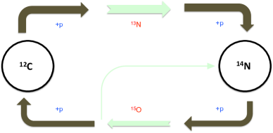
Figure 2: Scheme of the reactions of the CNO-I cycle. The light green arrows indicate the $\beta^{+}$ decay reactions that are tagged by neutrinos; the dark green arrows those that are not. The size of the arrows, not in scale, indicates the probability of the specific reactions. (The small internal arrow recalls us the existence of the CNO-II cycle.)

2.2 Another derivation of the luminosity constraint

Bahcall’s derivation of the luminosity constraint begins from the position,[1]

$$L_{\mathrel{{{\odot}}}}=4\pi\times\mbox{au}^{2}\times\sum_{i}\mathcal{Q}_{i}\times\Phi_{i}$$ (16)

The coefficients $\mathcal{Q}_{i}$ are the amount of light/heat associated to each of the 8 neutrino fluxes of the SSM, $\Phi_{i}$. We will show that a formal derivation of the coefficients $\mathcal{Q}_{i}$ leads again to cita1–see Eqs. (21,24,25-27) later on.

The reactions of the PP-chain and of the CNO-cycles, that allow the Sun to shine, can be grouped in 10 sequences, see tab-33. The PP-chain is divided in 6 sequences: 2 that form ³He and 4 that consume it, see fig3 for illustration. In the Sun, the CNO-cycle has two active sub-cycles, the CNO-I and the CNO-II; there are 2 sequences in each of them–those of the CNO-I sub-cycle are the upper and lower branches of fig2.

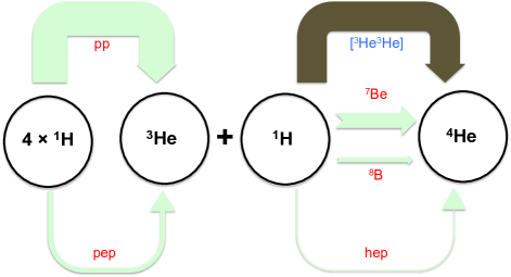
Figure 3: A representation of the sequences of the PP-chain in tab-33. The light green arrows indicate the sequences of reactions that are tagged by the 5 neutrino fluxes while the dark green arrow indicates the single sequence that is not tagged by neutrinos. Note the natural division of the PP-chain in the ³He formation (first part, fully tagged by pp and pep-neutrinos) and ³He consumption (second part, tagged only partly). The size of the arrows (not in scale) remind us the different probabilities of the sequences.

The values of the index $a$ that identify the 10 sequences are given in the 2${}^{\mbox{\tiny nd}}$ column of tab-33. Each sequence comprises various reactions (given in the $1^{\mbox{\tiny st}}$ column of tab-33) that are in kinetic equilibrium among them–i.e., all reactions have the same rate. Most sequences–8, out of 10–are associated to one specific neutrino flux: this allows us to measure the reaction rate $\dot{N}_{a}$ of each sequence, that is given by,

$$\color[rgb]{0,0,1}{{\dot{N}_{a}}={4\pi\times\mbox{au}^{2}}\times\Phi_{a}}$$ (17)

Consider now the amount of light/heat $\varepsilon_{a}$ produced in each sequence. The luminosity, usually measured in erg/s, can be written as,

$$L_{\mathrel{{{\odot}}}}=\sum_{a}\varepsilon_{a}\times\dot{N}_{a}$$ (18)

The values of $\varepsilon_{a}$ are given in the last column of tab-33 and are obtained as follows. The initial and final species of a sequence of reactions lead to energy release. This goes partly in kinetic energy or positrons (thus contributing to light/heat) and partly in the neutrino (being then lost):

$$\Delta M_{a}=\varepsilon_{a}+\langle E_{\nu}\rangle_{\!a}$$ (19)

where $\Delta M=M_{\mbox{\tiny initial}}-M_{\mbox{\tiny final}}$ is the difference of atomic masses in the sequence, given 4${}^{\mbox{\tiny th}}$ column of tab-33; the average energy losses $\langle E_{\nu}\rangle$ (5${}^{\mbox{\tiny th}}$ column of tab-33) are as in Bahcall.[2, 1, 11] Now we consider the two cases:

PP-chain: As emphasized in fig3, no physical neutrino flux is produced in the sequence 33. Still, this sequence can be associated to one formal neutrino flux, assuming with Bahcall[1] that the rate of formation of ³He in the PP-chain, $\dot{N}_{p1}+\dot{N}_{pe1}$, equates the rate of consumption of ³He, $2\times\dot{N}_{33}+\dot{N}_{e7}+\dot{N}_{p7}+\dot{N}_{p3}$. In other words, we extend defa introducing

$$\Phi_{33}\equiv\frac{\dot{N}_{33}}{4\pi\;\mbox{au}^{2}}=\frac{1}{2}(\Phi_{\mbox{\tiny pp}}+\Phi_{\mbox{\tiny pep}}-\Phi_{\mbox{\tiny Be}}-\Phi_{\mbox{\tiny B}}-\Phi_{\mbox{\tiny hep}})$$ (20)

This formal neutrino flux does not entail energy losses and can be evaluated from the observable fluxes of the PP-chain. Using Eqs. (17,19,20), we rearrange the first 6 terms of lefa as in lamantino finding,

$$\begin{array}[]{l}\mathcal{Q}_{\mbox{\tiny pp}}=\varepsilon_{p1}+\frac{\varepsilon_{33}}{2}=\frac{\mathcal{E}_{\mathrel{{{\odot}}}}}{2}-\langle E_{\mbox{\tiny pp}}\rangle\ ,\ \mathcal{Q}_{\mbox{\tiny pep}}=\varepsilon_{pe1}+\frac{\varepsilon_{33}}{2}=\frac{\mathcal{E}_{\mathrel{{{\odot}}}}}{2}-\langle E_{\mbox{\tiny pep}}\rangle,\\[1.29167pt] \mathcal{Q}_{\mbox{\tiny Be}}=\varepsilon_{p7}-\frac{\varepsilon_{33}}{2}=\frac{\mathcal{E}_{\mathrel{{{\odot}}}}}{2}-\langle E_{\mbox{\tiny Be}}\rangle\ ,\ \mathcal{Q}_{\mbox{\tiny B}}=\varepsilon_{e7}-\frac{\varepsilon_{33}}{2}=\frac{\mathcal{E}_{\mathrel{{{\odot}}}}}{2}-\langle E_{\mbox{\tiny B}}\rangle,\\[1.29167pt] \mathcal{Q}_{\mbox{\tiny hep}}=\varepsilon_{p3}-\frac{\varepsilon_{33}}{2}=\frac{\mathcal{E}_{\mathrel{{{\odot}}}}}{2}-\langle E_{\mbox{\tiny hep}}\rangle,\end{array}$$ (21)

where $\mathcal{E}_{\mathrel{{{\odot}}}}$ is as in epson and the other quantities are as in tab-33.

CNO-cycle: The O-neutrinos track mostly the CNO-I cycle and only in a minor amount the CNO-II cycle: $\Phi_{\mbox{\tiny O }}^{\mbox{\tiny I }}\gg\Phi_{\mbox{\tiny O }}^{\mbox{\tiny II }}$. In terms of the coefficients given in tab-33, the contribution to the luminosity of the CNO-cycle reads,

$$\frac{L_{\mathrel{{{\odot}}}}^{\mbox{\tiny CNO }}}{4\pi\times\mbox{au}^{2}}=\varepsilon_{p12}\;\Phi_{\mbox{\tiny N }}+\varepsilon_{p14}\;\Phi_{\mbox{\tiny O }}^{\mbox{\tiny I }}+\varepsilon_{p14^{\prime}}\;\Phi_{\mbox{\tiny O }}^{\mbox{\tiny II }}+\varepsilon_{p15}\;\Phi_{\mbox{\tiny F }}$$ (22)

Assume kinetic equilibrium for CNO-II, $\Phi_{\mbox{\tiny O}}=\Phi_{\mbox{\tiny O}}^{\mbox{\tiny I}}+\Phi_{\mbox{\tiny O}}^{\mbox{\tiny II}}$ and $\Phi_{\mbox{\tiny F}}=\Phi_{\mbox{\tiny O}}^{\mbox{\tiny II}}$; then, inserting the expressions for $\varepsilon_{a}$ from tab-33 and imelda, this becomes,

$$\frac{L_{\mathrel{{{\odot}}}}^{\mbox{\tiny CNO }}}{4\pi\times\mbox{au}^{2}}=\varepsilon_{p12}\;\Phi_{\mbox{\tiny N }}+\varepsilon_{p14}\;\Phi_{\mbox{\tiny O }}+(\varepsilon_{p12}+\langle E_{\mbox{\tiny N}}\rangle-\langle E_{\mbox{\tiny F}}\rangle)\;\Phi_{\mbox{\tiny F }}$$ (23)

Proceeding as for the PP chain and using Eqs. (19,23), we reorganize the 4 terms of the sum of lefa as in lamantino finding

$$\begin{array}[]{l}\mathcal{Q}_{\mbox{\tiny N}}=\varepsilon_{p12}={\mathcal{E}_{\mbox{\tiny C$\to$N}}}-\langle E_{\mbox{\tiny N}}\rangle\ ,\ \mathcal{Q}_{\mbox{\tiny O}}=\varepsilon_{p14}={\mathcal{E}_{\mathrel{{{\odot}}}}}-{\mathcal{E}_{\mbox{\tiny C$\to$N}}}-\langle E_{\mbox{\tiny O}}\rangle,\\ \mathcal{Q}_{\mbox{\tiny F}}=\varepsilon_{p12}+\langle E_{\mbox{\tiny N}}\rangle-\langle E_{\mbox{\tiny F}}\rangle={\mathcal{E}_{\mbox{\tiny C$\to$N}}}-\langle E_{\mbox{\tiny F}}\rangle,\end{array}$$ (24)

where $\mathcal{E}_{\mbox{\tiny C$\to$N}}$ is as in papibot. If one wants to omit the contribution of the CNO-II chain, describing the assumption that this is fully out of kinetic equilibrium (as Bahcall did[1]), it is enough to set $\Phi_{\mbox{\tiny F}}=0$.

Coefficients, in MeV, to express $L_{\mathrel{{{\odot}}}}$ as a function of the observable neutrino fluxes. The PP-chain The CNO-cycle pp Be pep B hep N O F $\mathcal{Q}_{i}^{\mbox{\tiny this work}}$ $\scriptstyle 13.0987$ $\scriptstyle 12.5525$ $\scriptstyle 11.9205$ $\scriptstyle 6.6305$ $\scriptstyle 3.7355$ $\scriptstyle 11.0075$ $\scriptstyle 14.0194$ $\scriptstyle 10.715$ $\mathcal{Q}_{i}^{\mbox{\tiny Bahcall}}$ $\scriptstyle 13.0987$ $\scriptstyle 12.6008$ $\scriptstyle 11.9193$ $\scriptstyle 6.6305$ $\scriptstyle 3.7370$ $\scriptstyle 3.4577$ $\scriptstyle 21.5706$ $\scriptstyle 0$ $\Delta\mathcal{Q}_{i}\times 1000$ $\scriptstyle 0$ $\scriptstyle 48.3$ $\scriptstyle-1.2$ $\scriptstyle 0$ $\scriptstyle 1.5$ $\scriptstyle-7549.8$ $\scriptstyle 7551.2$ $\scriptstyle-10715$

2.3 Improved values of the luminosity coefficients

At this point we can summarize. Let us begin recalling lamantino, namely,

$$L_{\mathrel{{{\odot}}}}=4\pi\times\mbox{au}^{2}\times\sum_{i}\mathcal{Q}_{i}\times\Phi_{i}\mbox{ with }{i=\mbox{\small pp,Be,pep,B,hep,N,O,F}}$$ (25)

where,

$$\left\{\begin{array}[]{lr}\mathcal{Q}_{i}=\mbox{light/heat associated to the $i$-th flux}&\mbox{[\ {\small MeV}\ ]}\\[-0.86108pt] \Phi_{i}=\mbox{observable solar neutrino fluxes}&\mbox{[\ {\small 1/(cm${}^{2}$s)}\ ]}\\[-0.86108pt] 4\pi\times\mbox{au}^{2}=4.50579\times 10^{21}&{[\ \mbox{\small erg cm}^{2}}/{\mbox{\small MeV}\ ]}\end{array}\right.$$ (26)

The numerical values of the coefficients $\mathcal{Q}_{i}$ calculated with tab-33 and Eqs. (21,24) are given in tabend: They are perfectly compatible with the outcomes of the SSM. In the same table one finds the values obtained by Bahcall.[1] Comparing the two sets of values, we note that,

1. Two contributions are in perfect agreement, those of pp- and B-fluxes.

2. Two differences are of trivial interpretation, namely, those of the pep- and hep-contributions, that are small and within roundoff errors.

3. The F-flux contribution to luminosity was simply omitted by Bahcall.

4. Some differences are non-trivial and need discussion: those of Be, N, O.

Treatment of Be-neutrinos: Two beryllium lines cause energy losses. The treatment advocated by Bahcall[1] requires two steps:

“one must average over the two ⁷Be neutrino lines with the appropriate weighting and include the $\gamma$-ray energy from the 10.3% of the decays that go to the first excited state of ⁷Li.”

(the emphasis on the word “and” is our choice and not in the original text).

In our understanding, Bahcall’s procedure is incorrect, for,

1. The energy loss of the EC on ⁷Be is due to a transition to the ground state in $\sim 90$% the cases, and to the one in the $1^{\mbox{\tiny st}}$ excited level in the rest; the average loss is thus $0.895\times 863.1+0.105\times 385.5=813.0$ keV as quoted in tab-33 (we updated $10.3\to 10.5$%, following Tilley et al 2002,[12] even though this is not crucial).

2. The gain of energy due to the $\gamma$-ray of 477.61 keV, emitted in 10.5% of the cases by the first excited state of ⁷Li, amounts to 50.1 keV. However, we do not include it as Bahcall does, for this amounts to double counting: to be sure, $863.1-813.0=50.1.$

Treatment of N- and O-neutrinos: The difference with Bahcall is in the choice of the sequences of the CNO-I cycle. In order to explain our choice, let us return to fig2. The two nuclear species there emphasized, ¹²C and ¹⁴N, have small S-factors and give rise to the slowest reactions of the CNO-I cycle; however, the ¹⁴N reaction is much slower, due to Coulomb suppression. When the cycle begins, N-neutrinos are soon produced and then ¹⁴N is synthesized. This is all that happens in the external part of the solar core, where the temperature is not too high: only half-cycle is active, only N-neutrinos are produced–see e.g., Fig. 2b of[13] and Fig. 1.2 right panel of.[14] In the inner part of the solar core, instead, the CNO-I cycle proceeds unimpeded and the N- and O-neutrinos are equally produced.

Summary: Eqs. (25,26,21,24) agree perfectly with cita1; in other words, the procedure advocated by Bahcall, with the new coefficients, leads to the same result that follows from physical considerations. The result, cita1, can be presented in compact form and in close resemblance to clitoi00,

$$\color[rgb]{0,0,1}{\sum_{i}\Phi_{i}\left(1-\frac{2\langle E_{i}\rangle}{\mathcal{E}_{\mathrel{{{\odot}}}}}\right)-0.123\times\delta\Phi_{\mbox{\tiny CNO}}=\frac{6.379\times 10^{10}}{\mbox{\small cm${}^{2}$s}}(1\pm 0.4\%)}$$ (27)

compare with Eqs. (3,8) and see clita for the $\delta\Phi_{\mbox{\tiny CNO}}$-term; note that according to the SSM, the $\delta\Phi_{\mbox{\tiny CNO}}$-contribution is below the present accuracy. fig2 and 3 remind us the physical conditions from nuclear physics,

$$\Phi_{i}\geq 0\ ,\ \Phi_{\mbox{\tiny pp}}+\Phi_{\mbox{\tiny pep}}\geq\Phi_{\mbox{\tiny Be}}+\Phi_{\mbox{\tiny B}}+\Phi_{\mbox{\tiny hep}}\ ,\ \Phi_{\mbox{\tiny N}}+\Phi_{\mbox{\tiny F}}\geq\Phi_{\mbox{\tiny O}}\geq\Phi_{\mbox{\tiny F}}$$ (28)

3 Flavor transformations of solar neutrinos

Before using the luminosity constraint, it is necessary to discuss a bit the interpretation of the observations of solar neutrino telescopes.

The original goal was to measure neutrino fluxes in order to understand the Sun, taking full advantage of the SSM (i.e., using and/or testing it). This goal is still valid and it is still pursued. It inspired the concept of the first solar neutrino experiment, Homestake, and of the most recent one, Borexino.

However, the experiments proved that solar neutrinos are modified by peculiar phenomena. Indeed, when neutrinos are produced in the Sun they have electronic flavor, but subsequently, when they reach the Earth, they are a combination of the various neutrino flavors–as first argued by Pontecorvo. An entire generation of solar neutrino observatories has worked to clarify the nature of these phenomena.

Nowadays the laws of flavor transformation are known and verified with independent terrestrial experiments, in particular with KamLAND. The most popular opinion is that these phenomena can be precisely described within a reasonable particle physics model where the three known neutrinos are endowed with mass. Thus, it is possible to return on the original goal, and use the solar neutrino experiments (along with the knowledge of flavor transformation phenomena) to reconstruct the emitted fluxes.

This is the position that we take in the rest of the present work: flavor transformation phenomena are supposed to be understood. In the appendix there is a somewhat broader discussion of the particle physics picture, with a brief mention of alternative models, which have some motivation but lack sufficient evidence to be considered too seriously for now. See also.[8, 16]

4 Applications

In this section, we consider various applications of the luminosity constraint, focussing in particular on its uses for the purpose of extracting the CNO signal–presumedly, the hottest issue in solar neutrino physics.[8]

4.1 A quasi-empirical model for the PP-chain

tab2 resumes the direct information on the fluxes of the PP-chain, where,
$\bullet$ the results on the pp-neutrinos obtained from the Gallium experiments[17] are averaged with the direct determination of Borexino;[18]
$\bullet$ the values of the Be- and pep-neutrinos are as measured by Borexino;[18]
$\bullet$ for the latter, the results from the two most recent SSM (with different metallicity) are averaged, enlarging the quoted error accordingly;
$\bullet$ the B-neutrinos flux measured by SNO is used (this is independent from assumptions on 3 flavor neutrino transformations, see again footnote 3);
$\bullet$ the hep-neutrino bound as derived by SNO[19] and Super-Kamiokande[20] is cited (SNO has a new analysis of hep-neutrinos in preparation);
$\bullet$ symmetric uncertainties are given for the purpose of illustration, even if their values should be considered with a grain of salt.

The quasi-empirical model of tab2 was defined as follows,
(1) the CNO-neutrinos are set to zero by definition;
(2) the precise value of pp-neutrinos follows from luminosity constraint, by applying a straightforward $\chi^{2}$ analysis;
(3) the ratio pep/pp fluxes was set to the theoretical value of $2.35\times 10^{-3}$ of,[21] including conservatively (but to some extent arbitrarily) a 2% error;
(4) the values of the Be- and pep-neutrinos stay unchanged;
(5) the value of the hep-neutrinos is set to the theoretical value, which incidentally gives a good fit to Super-Kamiokande data.[20]
This model is useful, since the luminosity constraint has a great impact on pp-neutrinos: the errors on the pp and the pep-neutrino fluxes decrease by one order of magnitude. The first hypothesis was considered also in the past[22] with different motivations; to date, the merit it has is of breaking the entanglement, that will be discussed in the next section.

Fluxes of the PP-chain and their uncertainties. $2^{\mbox{\tiny nd}}$ and $3^{\mbox{\tiny rd}}$ lines: current observational information. $4^{\mbox{\tiny th}}$ and $5^{th}$ lines: quasi-empirical model. We adopt the same notation as in ntn and in tab1. ident. index $i$ pp Be pep B hep observation 6.04 4.99 1.33 5.25 $<23$ errors 0.53 0.13 0.29 0.20 90% quasi-empirical 6.02 4.99 1.41 5.25 8 errors 0.03 0.13 0.03 0.20 9

4.2 Entanglement of PP and CNO-neutrino signals:

The luminosity constraint fixes precisely a linear combination of the various neutrino fluxes; the largest contribution in the SSM is due to the pp-neutrinos, followed by the one of the Be-neutrinos. In order to illustrate this point better, and using the notation of ntn, namely, $\Phi_{i}=\varphi_{i}\times 10^{\alpha_{i}}$/(cm²s), we explicitly include the order-of-magnitude factors (i.e., the values of $\alpha_{i}$ from tab1) obtaining

$$\begin{array}[]{c}0.9800\times\varphi_{\mbox{\tiny pp}}+0.0939\times\varphi_{\mbox{\tiny Be}}+0.0092\times\varphi_{\mbox{\tiny CNO}}+\\ +0.0089\times\varphi_{\mbox{\tiny pep}}+\mbox{\small small terms}=6.379\times(1\pm 0.4\%)\end{array}$$ (29)

The coefficient of the CNO-neutrinos depends upon the SSM in principle, but in practice it does not vary much–in agreement with the discussion after citabo.

This constraint can be exploited together with two recognized facts about solar neutrinos: 1) The Be-contribution is measured so precisely in Borexino,[18] that can be considered known; 2) the pep-contribution is strictly linked to the pp-one.[21] In this manner we find,

$$\color[rgb]{0,0,1}{\Phi_{\mbox{\tiny pp}}+0.93\times\Phi_{\mbox{\tiny CNO}}=6.02\times{10^{10}}{\mbox{(cm${}^{2}$ s)}}\times(1\pm 0.5\%)}$$ (30)

that improves[22, 23]. Thus, the central values of pp- and CNO-neutrino fluxes are almost fully anticorrelated, since it is just the above combination which is determined by the luminosity constraint. In fact, if we had not measured the neutrinos (but only the light), it would impossible to conclude on a firm observational ground that the Sun works mostly by the PP-chain.

4.3 Radiochemical experiments and the CNO-neutrinos

The measured rate at the Homestake (chlorine) experiment is

$$R_{\mbox{\tiny exp}}(\mbox{Cl})=2.56\pm 0.23\ \mbox{SNU}$$ (31)

The contributions in the quasi-empirical model, in order of importance, are,

$$\{\mbox{B},\mbox{Be},\mbox{pep,hep}\}=\{1.86,0.64,0.12,0.01\}\ \mbox{SNU}$$ (32)

The error on the cross section is estimated to be 3.7% for the high energy branches, B and hep, while it is 2% for the other neutrino fluxes;

$$R^{\mbox{\tiny PP}}_{\mbox{\tiny th}}(\mbox{Cl})=2.63\pm 0.08\mbox{ SNU}$$ (33)

namely it amounts to 3.2%. Therefore the rate of CNO-neutrinos, extracted from these data, is,

$$R^{\mbox{\tiny CNO}}_{\mbox{\tiny th}}(\mbox{Cl})=-0.07\pm 0.24$$ (34)

The measured rate from SAGE and Gallex/GNO is

$$R_{\mbox{\tiny exp}}(\mbox{Ga})=66.1\pm 3.1\ \mbox{SNU}$$ (35)

Expectations based on quasi-empirical model are in this case,

$$\{\mbox{pp},\mbox{Be},\mbox{B},\mbox{pep}\}=\{39.1,18.1,3.9,1.4\}\ \mbox{SNU}$$ (36)

The error on the cross section obtained using[17] (but see also[24]) implies,

$$R^{\mbox{\tiny PP}}_{\mbox{\tiny th}}(\mbox{Ga})=62.6^{+3.7}_{-1.9}\ \mbox{SNU}$$ (37)

absolute errors of pp, Be, B are almost equal and are summed linearly–not quadratically. Assuming, $R_{\mbox{\tiny exp}}(\mbox{Ga})=R^{\mbox{\tiny PP}}_{\mbox{\tiny th}}(\mbox{Ga})+R^{\mbox{\tiny CNO}}_{\mbox{\tiny th}}(\mbox{Ga})$ we find

$$R^{\mbox{\tiny CNO}}_{\mbox{\tiny th}}(\mbox{Ga})=3.5^{+3.6}_{-4.8}\ \mbox{SNU}$$ (38)

To improve, more data are needed and much more importantly, the theoretical error should be lessened by measuring the cross section.

4.4 Summary of what we know on CNO-neutrinos

The expected CNO-neutrino flux, deduced from tab1 and mab, is,

$$\varphi_{\mbox{\tiny CNO}}=4.88\mbox{ [GS98]},3.51\mbox{ [AGSS09]}$$ (39)

It depends upon the SSM. Borexino has searched for CNO-neutrinos: The 95% bound $\varphi_{\mbox{\tiny CNO}}<7.9$ was obtained scaling together the three fluxes, as predicted by the most recent SSM.[18] In their fig. 6 one finds the $\Delta\chi^{2}_{\mbox{\tiny Borexino}}(n)$ as a function of the counting rate $n_{\mbox{\tiny CNO}}$, obtained assuming the GS98 model. This is well-described by a parabolic shape, which implies that the likelihood is almost Gaussian. The minimum is at $n_{\mbox{\tiny CNO}}=2.4$ counts per day/100t, that corresponds to a flux $\varphi_{\mbox{\tiny CNO}}=2.34.$[18] Therefore, we have,

$$\Delta\chi^{2}_{\mbox{\tiny Borexino}}(\varphi_{\mbox{\tiny CNO}})=\frac{(\varphi_{\mbox{\tiny CNO}}-2.34)^{2}}{\delta\varphi^{2}}\mbox{ with }\delta\varphi=2.85$$ (40)

where the value of $\delta\varphi$ reproduces the quoted 95% bound and where we assume that the best fit value does not change drastically assuming the AGSS09 model instead. Summarizing, Borexino allows us to derive important empirical conclusions on the CNO-flux:

1. its value is lower than the one indicated by the GS98 and AGSS09 models;

2. within the upper 1$\sigma$ range, it is compatible with both of them;

3. within the lower 1$\sigma$ range, it is compatible with no CNO flux at all.

By combining the results of gallium experiments and Borexino, we find (for both SSM) a very mild shift upward $\varphi_{\mbox{\tiny CNO}}=2.69\pm 2.77$, that we quote as,

$$\color[rgb]{0,0,1}{\Phi_{\mbox{\tiny CNO}}=(2.69\pm 2.77)\times\frac{10^{8}}{\mbox{\small cm${}^{2}$s}}}$$ (41)

The important conclusions (1), (2), (3), outlined just above, remain valid. All this shows that the inclusion of the results of the gallium experiments in the analysis does not modify strongly the Borexino limit on CNO-neutrinos, which is the main information available today from the observations.

4.5 Future chances in Borexino and pep-neutrinos

As emphasized by D. Guffanti,[3], in the region of energies where CNO-neutrinos can give an observable signal, pep-neutrinos are present: Thus, this “beam-related background” should be known as precisely as possible, in order not to interfere with the extraction of the CNO bound (or signal).

One procedure that does not imply the theoretical input of the SSM, but only the usage of the luminosity constraint, is simply the following one: We can perform a global fit to the data using the luminosity constraint to determine the pp-neutrino flux accurately, moreover we can employ the known ratio between pep and pp[21] to fix pep-neutrinos reliably.

The theoretical error on this ratio is presumedly small; still, it would be useful to assess precisely its value in future. Indeed, even if the matrix element of the two reactions leading to pp- and pep-neutrinos is the same, $(i)$ pp- and pep-neutrinos are produced in slightly different regions, and $(ii)$ the description of electron capture requires theoretical modeling.

5 Discussion

Great results in solar neutrino astronomy have been obtained and new ones are expected: There is also a chance of measuring for the first time a signal from CNO-neutrinos, after those seen from the PP-neutrinos, thereby elucidating the two main astrophysical mechanisms that fuel stars.

The measured solar luminosity, with minimal theoretical inputs, leads to the luminosity constraint, that is based on the assumptions that the Sun is in equilibrium and we understand sufficiently well nuclear physics. This is a precious tool to proceed further in the study of the Sun; we have proposed an improved description and discussed it thoroughly.

The luminosity constraint and several other facts imply that the PP and CNO-neutrino signals are entangled, due to the empirical need to extract both of them from the experimental data. The apparently simplicity of this point should not lead us to underrate its importance; instead, it should be taken into account attentively in order to plan future steps forward at best.

We have examined various consequences of this situation: 1) The entanglement implies that it is momentous to probe CNO-neutrinos; Borexino has the best chances to fulfil this goal and it will indicate us the way to go. 2) The knowledge of the gallium cross section should be improved; its uncertainty hinders the chances of exploiting at best existing measurements. 3) Further work to measure the solar luminosity and to assess the connection between pp- and pep-fluxes would be desirable.

6 Acknowledgments

I thank M. Meyer and K. Zuber for the invitation, the German Alumni programme of TUM Dresden for support and in particular M. Richter-Babekoff and her staff for the very professional and friendly assistance. I am grateful to C. Mascaretti for collaboration in the early stage of this work and also to G. Bellini, M. Busso, I. Drachnev, M. Junker, A. Gallo Rosso, T. Kirsten, V. Gavrin, D. Guffanti, S. Marcocci, L. Marcucci, L. Pandola, G. Ranucci, A.Yu. Smirnov, D. Vescovi and D. Xue-Feng for pleasant discussions.

On flavor transformation of solar neutrinos

The phenomena of neutrino transformations are often called ‘neutrino oscillations’ see e.g.[25, 26] even when they do not have oscillatory character. This is true for solar neutrinos,[27] thus we refrain to use this terminology. Here, the reference model for these phenomena, based on the assumption that the three known neutrinos have small masses, is summarized, discussing briefly alternative schemes of interpretation. See the talks at Neutrino 2018[28] for updated information and also[8, 16] for a discussion that emphasizes the connections of neutrino transformations and solar neutrino astronomy.

The three flavor interpretation: It is a recognized fact that under suitable conditions neutrinos are subject to flavor transformations. The current interpretative framework can be summarized as follows: 1) there are 3 light species of neutrinos subject to weak interactions, $\nu_{\mbox{\tiny e}},\nu_{\mu},\nu_{\tau}$; 2) consistently with solar and atmospheric neutrino data, they undergo flavor transformations, i.e., the final flavor is not the initial one; 3) these phenomena are attributed to neutrino masses, and the parameters relevant for their description have been measured;[29] 4) this model was tested by means of reactor and accelerator experiments; 5) the assumption on the number and on the mass of the neutrinos is consistent with observational cosmology, namely, what we know from the $\Lambda$CDM cosmological model on big-bang nucleosynthesis and cosmic microwave background.

The current theory of solar neutrino transformations has been established since more than 30 years, when the matter - or MSW[25, 26] - effect was finally understood. Let us recall the main features of this theory: The hamiltonian of neutrino propagation includes, besides the term due to neutrino masses, also a further term–only for electron neutrinos–due to weak interactions with the electron in the medium: This is the matter term. Due to the matter term, the high energy solar neutrinos–such as the B-neutrinos–are produced as local-mass-eigenstates in the core of the Sun and exit as such, leading to the survival probability $P_{ee}=|U_{e2}^{2}|\sim 0.3$. The low energy solar neutrinos - as the pp-, Be- and pep-neutrinos - do not feel strongly the effect of the matter term and this leads to (phase averaged) flavor transformation in vacuum, $P_{ee}=\sum_{i=1}^{3}|U_{ei}^{4}|\sim 0.6$. This was reviewed in details by A. Smirnov,[3] discussing the formalism, the characteristic features and other manifestations, either observed or observable.

The parameters of flavor transformation indicated by a global interpretation of the data[29]–and more specifically the $\Delta m^{2}_{12}$ measured by the KamLAND experiment–lead to two expectations: a) the spectral shape should be distorted, so to grow at low energies–‘upturn’; b) the solar neutrinos that pass through the Earth, that have already undergone flavor transformation in the Sun, should undergo a small conversion back into electron neutrinos–‘regeneration’: but ‘upturn’ is not seen while ‘regeneration’ is larger than expected, see [20] and compare with Y. Suzuki.[3] Thus, even if the observed phenomena do not have a strong significance to date, the very detailed analysis of the B-neutrino flux of Super-Kamiokande suggests caution.

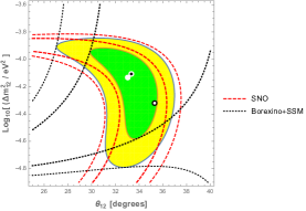
Figure 4: The oscillation probabilities obtained by the rates of SNO and Borexino lead to a best fit point - white circle dotted in black - that agrees very well with the global fit point - white circle. The point indicated by Super-Kamiokande measurements - with ‘upturn’ and ‘regeneration’ - is also shown for comparison - black circle dotted in white. From.[16]

On the other hand, it has been noted that, SNO and Borexino solar neutrino data allow us to reconstruct the ‘survival probability’ of the MSW theory, even omitting Super-Kamiokande data altogether; proceeding in this manner one finds a best fit point that agrees perfectly with the one indicated by the global analyses and by KamLAND[16] as shown in figQuat.

More on the rôle of the theory: In view of the historical discussions at our meeting,[3] it is appropriate to conclude with a few considerations on the impact of theoretical considerations in the discussion of solar neutrinos.

The ‘standard model’ of elementary particles led us to consider with favor the idea of three families, which implies the existence of three massless neutrinos subject to weak interactions. The most direct extension of this model includes non-renormalizable operators suppressed by large mass scales, that describe the effects of new physics[30] and endows the neutrinos of the standard model with small but non-zero masses.

The ensuing hypothesis of three light and massive neutrinos has been discussed and compared with the available data since the beginning. It results into a predictive model for flavor transformations: E.g., in 2001 there were ambiguities in the allowed parameters: using this model it was argued[10] that KamLAND and Borexino were enough to resolve them by measuring the relevant parameters, as it happened eventually.

The existence of other neutral fermions without weak interaction (e.g., ‘right-handed neutrinos) seems to be plausible; the real question concerns however the value of their mass, a parameter that in the context of the standard model has nothing to do with the electroweak scale and thus it is completely undetermined. A popular and reasonable position is that their mass is fixed by new gauge interactions at much higher scale. The converse assumption that some of these fermions is very light (and could play a rôle in the observed phenomena of flavor transformation) cannot be fully excluded, even if it lacks of convincing theoretical motivation to date.

Let us consider however the existence of a very light fourth neutrino, without weak interactions: a ‘sterile’ neutrino. Assuming that such a hypothetical particle has a non-negligible mixing with the other neutrinos, various individual anomalies can be addressed. However, no global analysis that has adopted a precisely defined model of this type has found significant evidence. Already the first one failed to find any significant hint.[31] A recent global analysis of M. Maltoni[28] indicates internal contradictions. This shows, once more, that well-formulated models are useful to interpret the data. Moreover, direct tests of the so-called ‘gallium anomaly’ and ‘reactor anomaly’, within simplified 2 flavor schemes, lead to disagreement with the DANSS, Stereo and NEOS experiments.[28]

Finally, one could speculate about new interactions felt only by neutrinos, or maybe by the new hypothetical neutrinos, that can lead to further matter effect, aka, non-standard interactions (NSI), as first argued in.[32, 33] This can help to address current anomalies of some experiments, however it is not clear that well-defined minimal models are viable, when one considers that the new interactions should show up in the phenomena of interest and also elsewhere, say, in collider or flavor experiments. In fact, the known neutrinos are part of leptonic doublets, e.g., $\ell_{e}=(\nu_{\mbox{\tiny e}},e)$, and the assumption of NSI implies also phenomena involving charged leptons.

Let us summarize: We have assumed the conventional 3 flavor description of neutrino transformation phenomena all throughout the present work. This is a description that has provided and that can provide us valid guidance in the discussion of the experimental findings. Different opinions follow, when excessive simplifications are adopted for the description of the data, or conversely when complicated theoretical schemes are adopted despite the weakness of their current motivations. For more discussion, see.[8, 16]

References

- [1] J. Bahcall, The luminosity constraint on solar neutrino fluxes, Phys. Rev. C 65, 025801 (2002)
- [2] J. Bahcall, Neutrino Astrophysics (Cambridge Univ. Press, UK, 1989)
- [3] 5 International Solar Neutrino Conference, Dresden (June 2018) https://indico.desy.de/indico/event/18666/
- [4] J. Bahcall and R.K. Ulrich, Solar models, neutrino experiments and helioseismology, Rev. Mod. Phys. 60, 297 (1988)
- [5] J. Bahcall, M.H. Pinsonneault and S. Basu, Solar models: Current epoch and time dependences, neutrinos, and helioseismological properties, Astrophys. J. 555, 990 (2001)
- [6] N. Vinyoles et al., A new generation of standard solar models, Astrophys. J. 835, 202 (2017)
- [7] A. Gallo Rosso, C. Mascaretti, A. Palladino and F. Vissani, Introduction to neutrino astronomy, Eur. Phys. J. Plus, 133 267 (2018)
- [8] F. Vissani, Solar neutrino physics on the beginning of 2017, Nucl. Phys. Atom. Energy 18, 5 (2017)
- [9] J. Perrin, Matière et lumière - Essai de synthèse de la mécanique chimique, Ann. Phys. 9, 5 (1919)
- [10] A. Strumia and F. Vissani, Which solar neutrino experiment after KamLAND and Borexino?, JHEP 0111, 048 (2001)
- [11] J. Bahcall website, 2005, http://www.sns.ias.edu/~jnb/
- [12] D.R. Tilley et al., Energy levels of light nuclei A=5, A=6, A=7, Nucl. Phys. A 708, 3 (2002)
- [13] V. Antonelli, L. Miramonti, C. Peña Garay, A. Serenelli, Solar Neutrinos, Adv. in HEP 2013, Article ID 351926 (2013)
- [14] N. Vinyoles Vergés, The Sun as a laboratory of particle physics, PhD thesis defended at Universitat Autònoma de Barcelona (2017)
- [15] H.H. Chen, Direct approach to resolve the solar neutrino problem, Phys. Rev. Lett. 55, 1534 (1985)
- [16] F. Vissani, Joint analysis of Borexino and SNO data and reconstruction of the survival probability, Nucl. Phys. Atom. Energy 18, 303 (2017)
- [17] J. Abdurashitov et al. [SAGE Collaboration], Measurement of the solar neutrino capture rate with gallium metal. III: Results for the 2002–2007 data-taking period, Phys. Rev. C 80, 015807 (2009)
- [18] M. Agostini et al. [Borexino Collaboration], First simultaneous precision spectroscopy of pp, 7Be, and pep solar neutrinos with Borexino Phase-II, arXiv:1707.09279 [hep-ex]
- [19] A. Bellerive et al. [SNO Collaboration] The Sudbury Neutrino Observatory, Nucl. Phys. B 908, 30 (2016)
- [20] K. Abe et al. [Super-Kamiokande Collaboration], Solar neutrino measurements in Super-Kamiokande-IV, Phys. Rev. D 94, 052010 (2016)
- [21] E. G. Adelberger et al., Solar fusion cross sections II: the PP-chain and CNO-cycles, Rev. Mod. Phys. 83, 195 (2011)
- [22] M. Spiro, D. Vignaud, Solar model independent neutrino oscillation signals in solar neutrino experiments?, Phys. Lett. B 242, 279 (1990)
- [23] S.A. Bludman, N. Hata, P. Langacker, Astrophysical solutions are incompatible with the solar neutrino data, Phys. Rev. D 49, 3622 (1994)
- [24] V. Barinov et al., Revised -gallium cross section and prospects of BEST to resolve the Gallium anomaly, Phys. Rev. D 97, 073001 (2018)
- [25] L. Wolfenstein, Neutrino oscillations in matter, Phys. Rev. D 17, 2369 (1978)
- [26] S.P. Mikheyev, A.Yu. Smirnov, Resonance amplification of oscillations in matter and spectroscopy of solar neutrinos, Sov. J. Nucl. Phys. 42, 913 (1986)
- [27] A.Yu. Smirnov, Solar neutrinos: Oscillations or no-oscillations?, arXiv: 1609.02386
- [28] 28 International Conference on Neutrino Physics and Astrophysics, Heidelberg (June 2018) https://www.mpi-hd.mpg.de/nu2018/
- [29] F. Capozzi, E. Lisi, A. Marrone and A. Palazzo, Current unknowns in the three neutrino framework, Prog. Part. Nucl. Phys. 102, 48 (2018)
- [30] S. Weinberg, Baryon and lepton nonconserving processes, Phys. Rev. Lett. 43, 1566 (1979)
- [31] M. Cirelli et al., Probing oscillations into sterile neutrinos with cosmology, astrophysics and experiments, Nucl. Phys. B 708, 215 (2005)
- [32] E. Roulet, MSW effect with flavor changing neutrino interactions, Phys. Rev. D 44, 935 (1991)
- [33] M.M. Guzzo, A. Masiero, S.T. Petcov, On MSW effect with massless neutrinos and no mixing in the vacuum, Phys. Lett. B 260, 154 (1991)