A local Benford Law for a class of arithmetic sequences

Abstract.

It is well-known that sequences such as the Fibonacci numbers and the factorials satisfy Benford’s Law; that is, leading digits in these sequences occur with frequencies given by $P(d)=\log_{10}(1+1/d)$, $d=1,2,\dots,9$. In this paper, we investigate leading digit distributions of arithmetic sequences from a local point of view. We call a sequence locally Benford distributed of order $k$ if, roughly speaking, $k$-tuples of consecutive leading digits behave like $k$ independent Benford-distributed digits. This notion refines that of a Benford distributed sequence, and it provides a way to quantify the extent to which the Benford distribution persists at the local level. Surprisingly, most sequences known to satisfy Benford’s Law have rather poor local distribution properties. In our main result we establish, for a large class of arithmetic sequences, a “best-possible” local Benford Law; that is, we determine the maximal value $k$ such that the sequence is locally Benford distributed of order $k$. The result applies, in particular, to sequences of the form $\{a^{n}\}$, $\{a^{n^{d}}\}$, and $\{n^{\beta}a^{n^{\alpha}}\}$, as well as the sequence of factorials $\{n!\}$ and similar iterated product sequences.

1. Introduction

1.1. Benford’s Law

Benford’s Law refers to the phenomenon that the leading digits in many real-world data sets tend to satisfy

(1.1) $$P(\text{leading digit is $d$})=\log_{10}\left(1+\frac{1}{d}\right),\quad d=1,2,\dots,9.$$

Thus, in a data set satisfying Benford’s Law, a fraction of $\log_{10}(1+1/1)$, or around $30.1\%$, of all numbers in the set have leading digit $1$ in their decimal representation, a fraction of $\log_{10}(1+1/2)\approx 17.6\%$ have leading digit $2$, and so on.

The peculiar first-digit distribution given by (1.1) was first observed in 1881 by the astronomer Simon Newcomb [16] in tables of logarithms. It did not receive much attention until some fifty years later when the physicist Frank Benford [2] compiled extensive empirical evidence for the ubiquity of this distribution across a wide range of real-life data sets. In a now classic table, Benford tabulated the distribution of leading digits in twenty different data sets, ranging from areas of rivers to numbers in street addresses and physical constants. Benford’s table shows good agreement with Benford’s Law for most of these data sets, and an even better agreement if all sources of data are combined into a single data set.

In recent decades, Benford’s Law has received renewed interest, in part because of its applications as a tool in fraud detection. Several books on the topic have appeared in recent years (see, e.g., [4], [14], [18]), and close to one thousand articles have been published (see [5]). For an overview of Benford’s Law, its applications, and its history we refer to the papers by Raimi [19] and Hill [10]. An in-depth survey of the topic can be found in the paper by Berger and Hill [3].

1.2. Benford’s Law for mathematical sequences

From a mathematical point of view, Benford’s Law is closely connected with the theory of uniform distribution modulo $1$ [11]. In 1976 Diaconis [7] used this connection to prove rigorously that Benford’s Law holds (in the sense of asymptotic density) for a class of exponentially growing sequences that includes the powers of $2$, $\{2^{n}\}$, the Fibonacci numbers, $\{F_{n}\}$, and the sequence of factorials, $\{n!\}$. That is, in each of these sequences, the asymptotic frequency of leading digits is given by (1.1).

In recent years, a variety of other (classes of) natural arithmetic sequences have been shown to satisfy Benford’s Law. In particular, in 2011 Anderson, Rolen and Stoehr [1] showed that Benford’s Law holds for the partition function $p(n)$ and for the coefficients of an infinite class of modular forms. In 2015, Massé and Schneider [13] established Benford’s Law for a class of fast-growing sequences defined by iterated product operations, including the superfactorials, $\prod_{k=1}^{n}k!$, the hyperfactorials, $\prod_{k=1}^{n}k^{k}$, and sequences of the form $2^{P(n)}$, where $P(n)$ is a polynomial. On the other hand, the validity of Benford’s Law for doubly exponential sequences such as $\{2^{2^{n}}\}$ or $\{2^{F_{n}}\}$ remains an open problem.

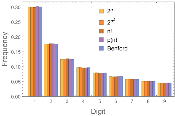
Figure 1. Frequencies of leading digits (in base $10$) among the first $10^{5}$ terms of the sequences $\{2^{n}\}$, $\{2^{n^{2}}\}$, $\{n!\}$, and $\{p(n)\}$, along with the frequencies given by the Benford distribution (1.1).

Figure 1 illustrates these results, showing the frequencies of leading digits for the sequences $\{2^{n}\}$, $\{2^{n^{2}}\}$, $\{n!\}$, and $\{p(n)\}$ (where $p(n)$ is the partition function). The leading digit frequencies of all four sequences are in excellent agreement with the frequencies predicted by Benford’s Law.

In contrast to these positive results, it has long been known (and is easy to see, e.g., by considering intervals of the form $[10^{k},2\cdot 10^{k})$) that sequences of polynomial (or slower) rate of growth such as $\{n\}$ or $\{n^{2}\}$ do not satisfy Benford’s Law in the usual asymptotic density sense. In many of these cases, Benford’s Law can be shown to hold in some weaker form, for example, with the natural asymptotic density replaced by other notions of density (see [12] for a survey).

1.3. Local Benford distribution

As Figure 1 shows, in terms of the global distribution of leading digits, the four sequences $\{2^{n}\}$, $\{2^{n^{2}}\}$, $\{n!\}$, and $\{p(n)\}$ all seem to behave in essentially the same way. This raises the question of whether one can distinguish between such leading digit sequences in some other way. For example, if we are given a block of consecutive leading digits from each of these four sequences, as in Table 1 below, can we tell, with a reasonable level of confidence, to which sequence each block belongs?

Sequence	Leading digits of first $50$ terms (concatenated)
$\{2^{n}\}$	2481361251 2481361251 2481361251 2481361251 2481371251
$\{2^{n^{2}}\}$	2156365121 2271519342 5412132118 1169511474 1146399353
$\{n!\}$	1262175433 3468123612 5126141382 8282131528 3162152163
$\{p(n)\}$	1235711234 5711122346 7111123345 6811112233 4567811112

Table 1. Leading digits (in base $10$) of the first $50$ terms of the sequences $\{2^{n}\}$, $\{2^{n^{2}}\}$, $\{n!\}$, and $\{p(n)\}$.

All four sequences in this table are known to satisfy Benford’s Law, so in terms of the global distribution of leading digits they behave in roughly the same way. This behavior is already evident in the limited data shown in Table 1. For example, among the first $50$ terms of the sequence $\{2^{n}\}$ exactly $15$ have leading digit $1$, while the digit $1$ counts for the other three sequences are $15$, $14$, and $18$, respectively. These counts are close to the counts predicted by Benford’s law, namely $50\cdot\log_{10}2\approx 15.05\dots$.

A closer examination of Table 1 reveals significant differences at the local level: The leading digits of $\{2^{n}\}$ exhibit an almost periodic behavior with a strong (and obvious) correlation between consecutive terms, while the sequence $\{p(n)\}$ shows a noticeable tendency of digits to repeat themselves. On the other hand, the leading digits of the sequences $\{2^{n^{2}}\}$ and $\{n!\}$ appear to behave more “randomly”, though it is not clear to what extent this randomness persists at the local level. Is one of the latter two sequences more “random” in some sense than the other?

In this paper we seek to answer questions of this type by studying the leading digit distribution of arithmetic sequences from a local point of view. More precisely, we will focus on the distribution of $k$-tuples of leading digits of consecutive terms in a sequence, and the question of when this distribution is asymptotically the same as that of $k$ independent Benford distributed random variables.

When viewed from such a local perspective, striking differences between sequences can emerge. This is illustrated in Figure 2, which shows the frequencies of (selected) pairs of leading digits for the same four sequences that we considered in Figure 1. In stark contrast to the single digit frequencies shown in Figure 1, the frequencies of pairs of leading digits vary widely from sequence to sequence.

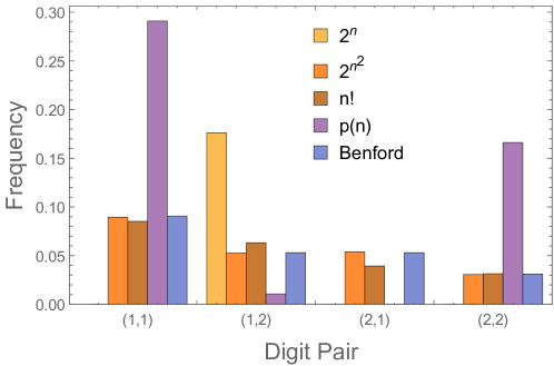
Figure 2. Frequencies of selected pairs $(d_{1},d_{2})$ of leading digits among the first $10^{5}$ terms of the sequences $\{2^{n}\}$, $\{2^{n^{2}}\}$, $\{n!\}$, and $\{p(n)\}$, along with the predicted frequencies, given by $P(d_{1})P(d_{2})=\log_{10}(1+1/d_{1})\log_{10}(1+1/d_{2})$. (Note that some of bars in the chart have height $0$ as the corresponding frequencies are $0$.)

Figure 2 suggests that for the sequence $\{2^{n^{2}}\}$ (but not for any of the other sequences in this figure) pairs of leading digits are distributed like independent Benford distributed random variables. Large scale computations of this sequence, shown in Table 2, provide compelling numerical evidence for this behavior.

$N$	$(1,1)$	$(1,2)$	$(2,1)$	$(2,2)$
$10^{4}$	0.0888777	0.054454	0.0552592	0.0312028
$10^{5}$	0.0894678	0.0528286	0.053985	0.0306747
$10^{6}$	0.0906688	0.0527907	0.0528264	0.0308901
$10^{7}$	0.0906353	0.052968	0.0529541	0.0309502
$10^{8}$	0.0906542	0.0529921	0.0529683	0.0310264
$10^{9}$	0.0906257	0.0530009	0.0530023	0.0310054
Benford	0.0906191	0.0530088	0.0530088	0.0310081

Table 2. Frequencies of selected pairs $(d_{1},d_{2})$ of leading digits among the first $N$ terms ($N=10^{k}$, $k=4,5,\dots,9$) of the sequence $\{2^{n^{2}}\}$, along with the predicted frequencies, given by $P(d_{1})P(d_{2})=\log_{10}(1+1/d_{1})\log_{10}(1+1/d_{2})$.

The results we will prove in this paper confirm the behavior suggested by Figure 2 and Table 2. We will show that, among the four sequences shown in Figures 1 and 2, only the sequence $\{2^{n^{2}}\}$ has the property that pairs of leading digits are distributed like independent Benford distributed variables. In this sense the sequence $\{2^{n^{2}}\}$ is the “most random” among these four sequences.

1.4. Summary of results and outline of paper

We call a sequence locally Benford distributed of order $k$ if, roughly speaking, $k$-tuples of leading digits of consecutive terms in this sequence are distributed like independent Benford-distributed digits (see Definition 2.1 below for a precise statement). This notion refines that of a Benford distributed sequence, which corresponds to the case $k=1$, and it provides a way to quantify the extent to which a Benford distributed sequence retains this property at the local level.

Given a Benford-distributed sequence (or, equivalently, a sequence that is locally Benford of order $1$), one can ask for the maximal value $k^{*}$ (if it exists) such that the sequence is locally Benford of order $k^{*}$. If such a value $k^{*}$ exists, we call $k^{*}$ the maximal local Benford order of the sequence; otherwise we say that the sequence has infinite maximal local Benford order.

Our main result, Theorem 2.8, determines this maximal local Benford order for a large class of arithmetic sequences that includes the main classes of sequences known to satisfy Benford’s Law. The result applies, in particular, to sequences of the form $\{a^{n}\}$, $\{a^{n^{d}}\}$, and $\{n^{\beta}a^{n^{\alpha}}\}$, as well as the factorials, the superfactorials, $\prod_{k=1}^{n}k!$, and similar iterated product sequences, and it allows us to classify these sequences according to their maximal local Benford order. For example, we will show (see Example 2.11(2)(4), Corollary 2.9, and Example 2.7(1) along with Theorem 2.8(ii)) that the sequences $\{2^{n}\}$, $\{n!\}$, and $\{p(n)\}$ have maximal local Benford order $1$ (so that, in particular, pairs of consecutive leading digits are not independent), while $\{2^{n^{2}}\}$ has maximal local Benford order $2$ (so that pairs of consecutive leading digits are independent, while triples are not). This answers the above question about the degree of “local randomness” in the four sequences shown in Table 1: The sequence $\{2^{n^{2}}\}$ is the most “random” of these sequences, in the sense of having the largest maximal Benford order.

The sequences covered by Theorem 2.8 all have finite maximal Benford order. To complement this result, we show in Theorem 2.13 the existence of sequences with infinite maximal local Benford order. Specifically, we consider doubly exponential sequences of the form $\{a^{\theta^{n}}\}$, where $a>1$. Using metric results from the theory of uniform distribution modulo $1$, we show that, for almost all real numbers $\theta>1$, such a sequence has infinite maximal local Benford order. We also show that when $\theta$ is an algebraic number, the sequence $\{a^{\theta^{n}}\}$ has finite maximal local Benford order, given by the degree of $\theta$ over $\mathbb{Q}$. The latter result applies, in particular, to the sequences $\{2^{2^{n}}\}$ and $\{2^{F_{n}}\}$, which are conjectured (but not known) to be Benford distributed. It shows that the maximal local Benford order of these sequences is at most $1$ in the case of $\{2^{2^{n}}\}$, and $2$ in the case of $\{2^{F_{n}}\}$.

The remainder of this paper is organized as follows. In Section 2, we introduce some notation and state our main results, Theorems 2.8 and 2.13, and some consequences and corollaries of these results. In Section 3, we introduce some background from the theory of uniform distribution modulo $1$ and we state our key tool, Proposition 3.5, a result on the uniform distribution modulo $1$ of $k$-tuples $(f(n),\dots,f(n+k-1))$, for certain classes of functions $f(n)$. We conclude this section by deducing Theorem 2.8 from Proposition 3.5. Section 4 is devoted to the proof of Proposition 3.5. Section 5 contains the proof of the corollaries of Theorem 2.8. Theorem 2.13 is proved in Section 6. The final section, Section 7, contains some remarks on related results and possible extensions and generalizations of our results.

2. Notation and statement of results

2.1. Notational conventions

Following the lead of most of the recent literature on Benford’s Law in a mathematical context, we consider leading digits with respect to expansions in a general base $b$, where $b$ is an integer $\geq 2$. The base $b$ analog of the Benford distribution (1.1) is given by

(2.1) $$P_{b}(d)=\log_{b}\left(1+\frac{1}{d}\right),\quad d=1,2,\dots,b-1.$$

The notations, definitions, and results we will introduce are understood to hold in this general setting. The dependence on $b$ may not be explicitly stated if it is clear from the context.

We let $\{a_{n}\}$ denote a sequence of positive real numbers, indexed by the natural numbers $n=1,2,\dots$. When convenient, we will use functional instead of subscript notation, and write a sequence as $\{f(n)\}$.

Given a real number $x$, we denote by $\lfloor x\rfloor$ (resp. $\lceil x\rceil$) the floor (resp. ceiling) of $x$, and we let $\{x\}=x-\lfloor x\rfloor$ denote the fractional part of $x$. (The curly brace notation is also used to denote sequences, but the meaning will always be clear from the context.)

We denote by $\log_{b}x$ the logarithm of $x$ in base $b$; that is, $\log_{b}x=(\log x)/(\log b)$.

We use the asymptotic notations $\sim$, $o(\dots)$, and $O(\dots)$, in the usual sense: $f(n)\sim g(n)$ means $\lim_{n\to\infty}f(n)/g(n)=1$; $f(n)=o(g(n))$ means $\lim_{n\to\infty}f(n)/g(n)=0$; and the notation $f(n)=O(g(n))$ means that there exists a constant $C$ (independent of $n$, but possibly depending on other parameters) such that $|f(n)|\leq C|g(n)|$ holds for all $n$.

Vectors and vector-valued functions are denoted by boldface symbols, and their components are indicated by subscripts, with indices starting at $0$. For example, $\mathbf{f}(n)=(f_{0}(n),\dots,f_{k-1}(n))$, $\mathbf{t}=(t_{0},\dots,t_{k-1})$. We denote by $\mathbf{0}$ the zero vector.

2.2. Local Benford distribution

Given a positive real number $x$ and an integer base $b\geq 2$, we let $d_{b}(x)$ denote the leading (i.e., most significant) digit of $x$ when expressed in base $b$. We then have, for any $d\in\{1,2,\dots,b-1\}$,

$$d_{b}(x)=d \Longleftrightarrow d\cdot b^{k}\leq x<(d+1)b^{k}\text{ for some $k\in\mathbb{Z}$ }$$

$$\Longleftrightarrow\log_{b}d\leq\{\log_{b}x\}<\log_{b}(d+1).$$

This equivalence relates the distribution of leading digits in base $b$ of a set of numbers $x$ to that of the fractional parts $\{\log_{b}x\}$. In particular, if these fractional parts are uniformly distributed in the interval $[0,1]$, then for each $d$ the proportion of numbers $x$ with leading digit $d$ will be $\log_{b}(d+1)-\log_{b}d=\log_{b}(1+1/d)$, i.e., the probability $P_{b}(d)$ given in (2.1). This motivates the following definition:

Definition 2.1 (Local Benford distribution).

Let $b$ be an integer base $\geq 2$, and let $\{a_{n}\}$ be a sequence of positive real numbers.

• The sequence $\{a_{n}\}$ is called Benford distributed with respect to base $b$ if

  (2.2) $$\lim_{N\to\infty}\#\frac{1}{N}\{n\leq N:\{\log_{b}a_{n}\}\leq\alpha\}=\alpha\quad(0\leq\alpha\leq 1).$$

• Let $k$ be a positive integer. The sequence $\{a_{n}\}$ is called locally Benford distributed of order $k$ with respect to base $b$ if

  (2.3) $$\lim_{N\to\infty} \#\frac{1}{N}\{n\leq N:\{\log_{b}a_{n+i}\}\leq\alpha_{i}\ (i=0,1,\dots,k-1)\}$$

  $$\qquad=\alpha_{0}\alpha_{1}\dots\alpha_{k-1}\quad(0\leq\alpha_{0},\alpha_{1},\dots,\alpha_{k-1}\leq 1).$$

Remarks 2.2.

(1) An alternative way to define a Benford distributed sequence would be to require the leading digits to have the asymptotic frequencies given by (2.1):

(2.4) $$\lim_{N\to\infty}\#\frac{1}{N}\{n\leq N:d_{b}(a_{n})=d\}=\log_{b}\left(1+\frac{1}{d}\right)\quad(d=1,\dots,b-1).$$

This amounts to restricting $\alpha$ in the given definition, (2.2), to the discrete values $\alpha=\log_{b}(d+1)$, $d=1,\dots,b-1$, and thus yields a slightly weaker property. Similarly, the notion of local Benford distribution could have been defined by the relation

(2.5) $$\lim_{N\to\infty} \#\frac{1}{N}\{n\leq N:d_{b}(a_{n+i})=d_{i}\ (i=0,1,\dots,k-1)\}$$

$$\qquad=\prod_{i=0}^{b-1}\log_{b}\left(1+\frac{1}{d_{i}}\right)\quad(d_{i}=1,\dots,b-1),$$

which would yield a slightly weaker property.

We decided to adopt the stronger definition, (2.2), as the basis for our concept of local Benford distribution since this is the definition most commonly used in the recent literature on the subject.

(2) In the case $k=1$, the definition of local Benford distribution, (2.3), reduces to that of the ordinary Benford distribution (2.2).

(3) It is immediate from the definition that local Benford distribution of order $k$ implies local Benford distribution of any smaller order $k^{\prime}<k$, and in particular implies Benford distribution in the sense of (2.2). As pointed out by the referee, a more general version of this observation holds: If a sequence $\{a_{n}\}$ is locally Benford distributed of order $k$, then for any integers $0\leq i_{1}<i_{2}<\dots<i_{h}\leq k$, the tuple $(a_{n+i_{1}},\dots,a_{n+i_{h}})$ behaves like a tuple of independent Benford distributed random variables.

Definition 2.3 (Maximal local Benford order).

Let $b$ be an integer base $\geq 2$ and let $\{a_{n}\}$ be a sequence of positive real numbers that is Benford distributed with respect to base $b$ (and hence also locally Benford distributed of order at least $1$).

• If there exists a maximal integer $k^{*}$ such that $\{a_{n}\}$ is locally Benford distributed of order $k^{*}$, then we call $k^{*}$ the maximal local Benford order of the sequence $\{a_{n}\}$ with respect to base $b$.

• If no such integer $k^{*}$ exists (i.e., if $\{a_{n}\}$ is locally Benford distributed of any order), we say that $\{a_{n}\}$ has infinite maximal local Benford order with respect to base $b$.

2.3. The classes $C_{k,i}$

Let $\Delta$ be the difference operator (or discrete derivative) defined by

(2.6) $$\Delta f(n)=f(n+1)-f(n),$$

and let $\Delta^{k}$ denote the $k$-th iterate of this operator, so that

(2.7) $$\Delta^{1}f(n)=\Delta f(n),\quad\Delta^{k+1}f(n)=\Delta(\Delta^{k}f(n))\quad(k=1,2,\dots).$$

We classify sequences $\{f(n)\}$ into classes $C_{k,i}$ according their asymptotic behavior under this iterated difference operator:

Definition 2.4 (Classes $C_{k,i}$).

Let $\{f(n)\}$ be a sequence of real numbers and let $k$ be a positive integer. We say that $\{f(n)\}$ is of

• class $C_{k,0}$ if for some $\theta\not\in\mathbb{Q}$,

  $$\lim_{n\to\infty}\Delta^{k}f(n)=\theta;$$

• class $C_{k,\alpha}$, where $0<\alpha<1$, if for some $\lambda\not=0$,

  $$\lim_{n\to\infty}n^{\alpha}\Delta^{k}f(n)=\lambda;$$

• class $C_{k,1}$, if for some $\lambda\not=0$,

  $$\lim_{n\to\infty}n\Delta^{k+1}f(n)=\lambda.$$

We denote by $C_{k,i}$ any of the three classes (i)–(iii).

Roughly speaking, class $C_{k,0}$ covers functions of growth proportional to $n^{k}$ and with irrational leading coefficient, class $C_{k,\alpha}$ covers functions of growth proportional to $n^{\beta}$, where $\beta>0$ is not an integer, while class $C_{k,1}$ covers functions of growth proportional to $n^{k}\log n$.

Remarks 2.5.

(1) Note that the definition of the class $C_{k,1}$ involves the $(k+1)$st iterate of the $\Delta$ operator, whereas the other two classes involve the $k$th iterate. This convention will allow us to state our results in a uniform manner for all three classes.

(2) It is not hard to see that a sequence $\{f(n)\}$ can belong to at most one of the classes $C_{k,i}$; that is, both $k$ and the class subscript $i$ are uniquely determined by the sequence $\{f(n)\}$. For example, suppose $f$ is of class $C_{k,0}$ for some $k\in\mathbb{N}$. Then

$$\Delta^{k+1}f(n)=\Delta^{k}f(n+1)-\Delta^{k}f(n)\to\theta-\theta=0,$$

and inductively we get $\Delta^{k+i}f(n)\to 0$ for all $i\geq 1$. Thus $f$ cannot be of class $C_{k^{\prime},0}$ for some $k^{\prime}>k$. Interchanging the roles of $k^{\prime}$ and $k$, we see that $f$ also cannot be of class $C_{k^{\prime},0}$ for some $k^{\prime}<k$. Hence, a sequence $\{f(n)\}$ can be in class $C_{k,0}$ for a most one value of $k$. Using similar reasoning one can show that $k$ is uniquely determined for sequences in the other two classes, $C_{k,\alpha}$ and $C_{k,1}$, and that a sequence can belong to at most one such class.

(3) It is clear from the definition that $\{\Delta f(n)\}$ belongs to $C_{k,i}$ if and only if $\{f(n)\}$ belongs to $C_{k+1,i}$. More generally, for any positive integer $h$ the sequence $\{\Delta^{h}f(n)\}$ belongs to $C_{k,i}$ if and only if the sequence $\{f(n)\}$ belongs to $C_{k+h,i}$.

(4) A sufficient condition for $f$ to be in some class $C_{k,i}$ is that $f$ is a function defined on $[1,\infty)$ satisfying the continuous analog of the given condition, i.e., with the $k$-th discrete derivative $\Delta^{k}f(n)$ replaced by the ordinary $k$-th derivative $f^{(k)}(x)$. To see this, note that if $f$ has continuous derivatives up to order $k$, then $\Delta^{k}f$ can be represented as an integral over the $k$-th derivative of $f$ of the form $(*)$ $\Delta^{k}f(n)=\int_{0}^{k}f^{(k)}(n+t)\phi_{k}(t)dt$, where $\phi_{k}(t)$ is a nonnegative kernel function supported on $[0,k]$ that integrates to $1$. The identity $(*)$ can be proved by induction.

Using the last of these remarks easily yields a large class of examples of functions belonging to one of the classes $C_{k,i}$:

Example 2.6.

• For any nonconstant polynomial $P(x)$ with irrational leading coefficient, $\{P(n)\}$ is of class $C_{k,0}$ with $k=\deg(P)$. In particular, $\{\theta n^{k}\}$ is of class $C_{k,0}$ whenever $\theta$ is irrational.

• For any nonconstant polynomial $P(x)$, the sequence $\{P(n)\log n\}$ is of class $C_{k,1}$ with $k=\deg(P)$. In particular, $\{n^{k}\log n\}$ is of class $C_{k,1}$.

• For any positive real number $\beta$ that is not an integer, the sequence $\{n^{\beta}\}$ is of class $C_{k,\alpha}$ with $k=\lceil\beta\rceil$ and $\alpha=k-\beta$.

2.4. Iterated product sequences

Given a sequence $\{a_{n}\}$, we define the iterated product sequences $\{a_{n}^{(h)}\}$ by (cf. [13])

(2.8) $$a_{n}^{(1)}=a_{n},\quad a_{n}^{(h+1)}=\prod_{m=1}^{n}a_{m}^{(h)}\quad(h=1,2,\dots).$$

Example 2.7.

• If $a_{n}=n!$, then the numbers $n!^{(2)}=\prod_{m=1}^{n}m!$ are the superfactorials, and the numbers $n!^{(h)}$ are generalized superfactorials, obtained by iterating the product operation.

• If $a_{n}=a^{P(n)}$, where $P$ is a polynomial of degree $d$, then $a_{n}^{(h)}=a^{P_{h}(n)}$, where $P_{h}(n)$ is a polynomial of degree $d+h-1$, defined inductively by $P_{1}(n)=P(n)$ and $P_{h+1}(n)=\sum_{m=1}^{n}P_{h}(m)$.

2.5. Statement of results

With the above definitions, we are ready to state our main result.

Theorem 2.8 (Main Theorem).

Let $b$ be an integer base $\geq 2$, let $\{a_{n}\}$ be a sequence of positive real numbers, and suppose the sequence $\{\log_{b}a_{n}\}$ belongs to one of the classes $C_{k,i}$ in Definition 2.4. Then:

• The sequence $\{a_{n}\}$ has maximal local Benford order $k$ with respect to base $b$; that is, $\{a_{n}\}$ is locally Benford distributed of order $k$, but not of any higher order.

• For any positive integer $h$, the iterated product sequences $\{a_{n}^{(h)}\}$ has maximal local Benford order $k+h-1$ with respect to base $b$.

The conditions on $\{a_{n}\}$ in this theorem are general enough to cover most of the classes of functions previously considered in the literature. In the following corollaries we give some special cases and consequences of this result.

Our first corollary is motivated by applications to the partition function and coefficients of modular forms (see [1]).

Corollary 2.9.

Suppose

(2.9) $$a_{n}\sim\lambda n^{\gamma}e^{cn^{\beta}},$$

where $\lambda,\gamma,c,\beta$ are constants with $\lambda>0,c>0,\beta>0$, and $\beta$ not an integer. Then $\{a_{n}\}$ has maximal local Benford order $\lceil\beta\rceil$ with respect to any base $b\geq 2$.

In particular, since the partition function $p(n)$ satisfies a relation of the form (2.9) with $\beta=1/2$, the corollary shows that $\{p(n)\}$ has maximal local Benford order $\lceil 1/2\rceil=1$ with respect to any base $b\geq 2$. Thus, while the leading digits of the partition function are Benford distributed (as previously shown in [1]), pairs of leading digits of consecutive terms do not behave like independent Benford distributed digits.

The next corollary concerns a very wide class of functions introduced in [13] (see Definition 3.4 and Theorem 3.10 of [11]) that includes, for example, sequences of geometric growth such as $\{2^{n}\}$ and the Fibonacci sequence $\{F_{n}\}$, and sequences of “super-geometric” growth such as $\{a^{n^{d}}\}$, as well as the sequence of factorials and similar functions such as $\{n^{n}\}$.

Corollary 2.10.

Let $b$ be an integer base $\geq 2$ and suppose

(2.10) $$a_{n}\sim\lambda n^{P(n)}b^{Q(n)},$$

where $P$ and $Q$ are polynomials and $\lambda>0$.

• If $\deg(P)<\deg(Q)$ and $Q$ has irrational leading coefficient, then $\{a_{n}\}$ has maximal local Benford order $k=\deg(Q)$ with respect to base $b$.

• If $\deg(P)\geq\deg(Q)$ and $P$ is nonconstant, then $\{a_{n}\}$ has maximal local Benford order $k=\deg(P)$ with respect to base $b$.

We mention some particular cases of this result:

Example 2.11.

1. The sequence $\{n^{n}\}$ satisfies (2.10) with $\lambda=1$, $P(n)=n$ and $Q(n)=0$, so by part (ii) of the corollary this sequence has maximal local Benford order $1$.

2. By Stirling’s formula we have $n!\sim\sqrt{2\pi}n^{n+1/2}e^{-n}$, so the factorial sequence $\{n!\}$ satisfies (2.10) with $P(n)=n+1/2$ and $Q(n)=-(1/\log b)n$. Thus, part (ii) of the corollary applies again and yields that $\{n!\}$ has maximal local Benford order $1$.

3. By Binet’s Formula, we have $F_{n}\sim(1/\sqrt{5})\Phi^{n}$, where $\Phi=(\sqrt{5}+1)/2$, so the Fibonacci sequence $\{F_{n}\}$ satisfies (2.10) with $P(n)=0$ and $Q(n)=(\log_{b}\Phi)n$. The leading coefficient of $Q$, $\log_{b}(\sqrt{5}+1)/2$, is irrational for any integer $b\geq 2$, so by part (i) of the corollary $\{F_{n}\}$ has maximal local Benford order $1$ with respect to any base $b\geq 2$.

4. The sequence $\{2^{n^{d}}\}$, where $d$ is a positive integer, satisfies (2.9) with $P(n)=0$ and $Q(n)=(\log_{b}2)n^{d}$. By part (i) of the corollary it follows that this sequence has maximal local Benford order $d$ with respect to any base $b$ such that $\log_{b}2$ is irrational, i.e., any base $b$ that is not a power of $2$.

The above special cases include the sequences in Figures 1 and 2 Table 1, and they allow us to resolve the question on the degree of “local randomness” in these sequences we had posed in the introduction: By Corollary 2.9 the sequence $\{p(n)\}$ has maximal local Benford order $1$. By Example 2.11, the sequences $\{n!\}$ and $\{2^{n}\}$ have maximal local Benford order $1$, while the sequence $\{2^{n^{2}}\}$ has maximal local Benford order $2$. Thus, pairs of leading digits of consecutive terms of $\{2^{n^{2}}\}$ behave like independent Benford-distributed random variables, while this is not the case for the sequences $\{2^{n}\}$, $\{n!\}$, and $\{p(n)\}$. In this sense, the sequence $\{2^{n^{2}}\}$ is the most “random” of the four sequences.

Corollary 2.12.

For any positive integer $n$, the generalized superfactorial sequence (see Definition 2.8), $\{n!^{(h)}\}$, has maximal local Benford order $h$ with respect to any base $b\geq 2$.

In all of the above examples the sequence has finite maximal local Benford order. One can ask if there exist sequences that have infinite local Benford order, i.e., sequences that are locally Benford distributed for any order $k$. The above results suggest that the order of local Benford distribution is closely related to the rate of growth of the sequence $\log_{b}a_{n}$. For example, if $\log_{b}a_{n}$ is a polynomial of degree $d$ with irrational leading coefficient, then $\{a_{n}\}$ has maximal local Benford order $d$. Hence one might expect that sequences for which $\log_{b}a_{n}$ grows at exponential rate “typically” will have infinite maximal local Benford order. The following result confirms this by showing that, in some sense, almost all sequences for which $\log_{b}a_{n}$ grows at an exponential rate have infinite local Benford order.

Theorem 2.13 (Local Benford order of doubly exponential sequences).

Let $a>1$ be a real number.

• For almost all real numbers $\theta>1$ the sequence $\{a^{\theta^{n}}\}$ has infinite maximal local Benford order with respect to any base $b\geq 2$.

• If $\theta>1$ is an algebraic number of degree $k$, then, with respect to any base $b$, the maximal local Benford order of the sequence $\{a^{\theta^{n}}\}$ is at most $k$.

Example 2.14.

• The sequence $\{2^{2^{n}}\}$ satisfies the conditions of Theorem 2.13(ii) with $\theta=2$. Since $2$ is algebraic of degree $1$, the theorem shows that the sequence cannot be locally Benford distributed of order $2$ (or greater). (Whether the sequence is locally Benford distributed of order $1$, i.e., whether it satisfies Benford’s Law, remains an open question.)

• By Binet’s Formula, we have

  (2.11) $$2^{F_{n}}\sim 2^{(1/\sqrt{5})\Phi^{n}},$$

  where $F_{n}$ denotes the $n$-th Fibonacci number and $\Phi=(\sqrt{5}+1)/2$. Since $\Phi$ is algebraic of degree $2$, the theorem can be applied to the sequence on the right of (2.11), and it shows that this sequence cannot be locally Benford distributed of order $3$ (or greater). In view of the relation (2.11) the same is true for the sequence $\{2^{F_{n}}\}$ (cf. Lemma 5.2 below).

3. Uniform distribution modulo 1 and the Key Proposition

In this section, we introduce some key concepts and results from the theory of uniform distribution modulo $1$, and we use these to reduce Theorem 2.8 to a statement about uniform distribution modulo $1$, Proposition 3.5 below. The proposition will be proved in the next section.

3.1. Uniform distribution modulo $1$ in $\mathbb{R}^{k}$

We recall the standard definition of uniform distribution modulo $1$ of sequences of real numbers, and its higher-dimensional analog; see, for example, Definitions 1.1 and 6.1 in Chapter 1 of [11].

Definition 3.1 (Uniform distribution modulo $1$ in $\mathbb{R}^{k}$).

• A sequence $\{f(n)\}$ of real numbers is said to be uniformly distributed modulo $1$ if

  (3.1) $$\lim_{N\to\infty}\frac{1}{N}\#\{n\leq N:\{f(n)\}\leq\alpha\}=\alpha\quad(0\leq\alpha\leq 1).$$

  (Recall that $\{x\}$ denotes the fractional part of $x$.)

• A sequence $\{\mathbf{f}(n)\}=\{(f_{0}(n),\dots,f_{k-1}(n))\}$ in $\mathbb{R}^{k}$ is said to be uniformly distributed modulo $1$ in $\mathbb{R}^{k}$ if

  (3.2) $$\lim_{N\to\infty}\frac{1}{N}\#\{n\leq N:\{f_{i}(n)\}\leq\alpha_{i}\ (i=0,1,\dots,k-1)\}$$

  $$\qquad=\alpha_{0}\alpha_{1}\dots\alpha_{k-1}\quad((\alpha_{0},\alpha_{1}\dots,\alpha_{k-1})\in[0,1]^{k}).$$

A key result in uniform distribution modulo $1$ is Weyl’s Criterion, which we will state in the following form; see Theorems 2.1, 6.2, and 6.3 in Chapter 1 of [11].

Lemma 3.2 (Weyl’s Criterion in $\mathbb{R}^{k}$).

• A sequence $\{f(n)\}$ of real numbers is uniformly distributed modulo $1$ if and only if

  (3.3) $$\lim_{N\to\infty}\frac{1}{N}\sum_{n=1}^{N}e^{2\pi itf(n)}=0\quad(t\in\mathbb{Z}\setminus\{0\}).$$

• A sequence $\{\mathbf{f}(n)\}=\{(f_{0}(n),\dots,f_{k-1}(n))\}$ in $\mathbb{R}^{k}$ is uniformly distributed modulo $1$ in $\mathbb{R}^{k}$ if and only if

  (3.4) $$\lim_{N\to\infty}\frac{1}{N} \sum_{n=1}^{N}\exp\left\{2\pi i(t_{0}f_{0}(n)+\dots+t_{k-1}f_{k-1}(n))\right\}=0$$

  $$\qquad\quad((t_{0},\dots,t_{k-1})\in\mathbb{Z}^{k}\setminus\{\mathbf{0}\}).$$

• A sequence $\{\mathbf{f}(n)\}=\{(f_{0}(n),\dots,f_{k-1}(n))\}$ in $\mathbb{R}^{k}$ is uniformly distributed modulo $1$ in $\mathbb{R}^{k}$ if and only if, for any vector $(t_{0},\dots,t_{k-1})\in\mathbb{Z}^{k}\setminus\{\mathbf{0}\}$, the sequence $\{t_{0}f_{0}(n)+\dots+t_{k-1}f_{k-1}(n)\}$ is uniformly distributed modulo $1$.

Part (iii) of this result is obtained by combining the $k$-dimensional Weyl criterion in (ii) with the one-dimensional Weyl criterion in (i), applied to the sequence $\{t_{0}f_{0}(n)+t_{1}f_{1}(n)+\dots+t_{k-1}f_{k-1}(n)\}$.

We next state the special case of the $k$-dimensional Weyl’s Criterion when $\mathbf{f}$ is of the form $\mathbf{f}(n)=(f(n),f(n+1),\dots,f(n+k-1))$, where $\{f(n)\}$ is a given sequence of real numbers. It will be convenient to introduce the notation

(3.5) $$f_{\mathbf{t}}(n)=\sum_{i=0}^{k-1}t_{i}f(n+i),$$

where $\mathbf{t}=(t_{0},t_{1},\dots,t_{k})$ is any $k$-dimensional vector. By applying (iii) of Lemma 3.2 with $\mathbf{f}(n)=(f(n),f(n+1),\dots,f(n+k-1))$, we obtain:

Corollary 3.3 (Weyl’s Criterion for $\{(f(n),f(n+1),\dots f(n+k-1))\}$).

Let $\{f(n)\}$ be a sequence of real numbers, and let $k$ be a positive real number. Then $\{(f(n),f(n+1),\dots,f(n+k-1))\}$ is uniformly distributed modulo $1$ in $\mathbb{R}^{k}$ if and only if, for each $\mathbf{t}\in\mathbb{Z}^{k}\setminus\{\mathbf{0}\}$, the sequence $\{f_{\mathbf{t}}(n)\}$ is uniformly distributed modulo $1$.

3.2. Local Benford distribution and uniform distribution modulo $1$

The following lemma characterizes local Benford distribution in terms of uniform distribution modulo $1$.

Lemma 3.4 (Local Benford distribution and uniform distribution modulo $1$).

Let $b$ be an integer base $\geq 2$, let $\{a_{n}\}$ be a sequence of positive real numbers, and let $f(n)=\log_{b}a_{n}$.

• The sequence $\{a_{n}\}$ is Benford distributed with respect to base $b$ if and only if the sequence $\{f(n)\}$ is uniformly distributed modulo $1$.

• Let $k$ be a positive integer. The sequence $\{a_{n}\}$ is locally Benford distributed of order $k$ with respect to base $b$ if and only if, for each $\mathbf{t}\in\mathbb{Z}^{k}\setminus\{\mathbf{0}\}$, the sequence $\{f_{\mathbf{t}}(n)\}$ is uniformly distributed modulo $1$.

Proof.

Assertion (i) is simply a restatement of the definition (2.2) of a Benford distributed sequence.

For the proof of (ii), we note that the definition (2.3) of a locally Benford distributed sequence sequence $\{a_{n}\}$ is exactly equivalent to the definition of uniform distribution modulo $1$ of the $k$-dimensional sequence $\{(f(n),f(n+1),\dots,f(n+k-1))\}$, with $f(n)=\log_{b}a_{n}$. By Corollary 3.3 this in turn is equivalent to the uniform distribution modulo $1$ of all sequences $\{f_{\mathbf{t}}(n)\}$, with $\mathbf{t}\in\mathbb{Z}^{k}\setminus\{\mathbf{0}\}$. ∎

3.3. The Key Proposition

We are now ready to recast our main result, Theorem 2.8, in terms of uniform distribution modulo $1$.

Proposition 3.5.

Let $k$ be a positive integer and let $\{f(n)\}$ be a sequence belonging to one of the classes $C_{k,i}$ in Definition 2.4. Then:

• For each $k$-dimensional vector $\mathbf{t}\in\mathbb{Z}^{k}\setminus\{\mathbf{0}\}$, the sequence $\{f_{\mathbf{t}}(n)\}$ is uniformly distributed modulo $1$.

• There exists a $(k+1)$-dimensional vector $\mathbf{t}\in\mathbb{Z}^{k+1}\setminus\{0\}$ such that the sequence $\{f_{\mathbf{t}}(n)\}$ is not uniformly distributed modulo $1$.

Franklin [8] established a result of the above type in the case when $f(n)$ is a polynomial with irrational leading coefficient. It is easy to see that in this case we have $\Delta^{k}f(n)=k!a_{k}$, where $k$ is the degree of $f(n)$ and $a_{k}$ is its leading coefficient, so $f(n)$ trivially belongs to the class $C_{k,0}$. Thus, Proposition 3.5 can be viewed as a far-reaching generalization of Franklin’s result.

3.4. Deduction of Theorem 2.8 from Proposition 3.5

Let $b$ be an integer base $\geq 2$, and let $\{a_{n}\}$ be a sequence of positive real numbers satisfying the assumptions of the theorem, so that the sequence $f(n)=\log_{b}a_{n}$ belongs to one of the classes $C_{k,i}$ in Definition 2.4 for some $k$. By Proposition 3.5 it follows that $\{f_{\mathbf{t}}(n)\}$ is uniformly distributed modulo $1$ for all $k$-dimensional vectors $\mathbf{t}\in\mathbb{Z}^{k}\setminus\{\mathbf{0}\}$, but not for all $(k+1)$-dimensional vectors $\mathbf{t}\in\mathbb{Z}^{k+1}\setminus\{\mathbf{0}\}$. By Lemma 3.4 it follows that $\{a_{n}\}$ is locally Benford of order $k$, but not of order $k+1$. This establishes part (i) of the theorem.

To prove part (ii), let $f^{(h)}(n)=\log_{b}a_{n}^{(h)}$, so that in particular $f^{(1)}(n)=f(n)$. Then, by the definition (2.8) of the iterated products, we have, for any $h\geq 2$,

$$f^{(h)}(n) =\log_{b}a_{n}^{(h)}=\log_{b}\prod_{m=1}^{n}a_{m}^{(h-1)}$$

$$=\sum_{m=1}^{n}\log_{b}a_{m}^{(h-1)}=\sum_{m=1}^{n}f^{(h-1)}(m),$$

and hence

$$\Delta f^{(h)}(n)=f^{(h)}(n+1)-f^{(h)}(n)=f^{(h-1)}(n+1).$$

By iteration we obtain

$$\Delta^{h-1}f^{(h)}(n)=f^{(1)}(n+h-1)=f(n+h-1)$$

and hence

(3.6) $$\Delta^{h+k-1}f^{(h)}(n)=\Delta^{k}f(n+h-1).$$

By the assumptions of the theorem, the sequence $\{f(n)\}$, and hence also the shifted sequence $\{f(n+h-1)\}$, satisfies one of the asymptotic conditions defining the classes $C_{k,i}$. By (3.6), it follows that the sequence $\{f^{(h)}(n)\}$ satisfies the same condition with $k$ replaced by $k+h-1$, and hence belongs to one of the classes $C_{k+h-1,i}$. Applying again Proposition 3.5 and Lemma 3.4 we conclude that $\{a_{n}^{(h)}\}$ is locally Benford of order $k+h-1$, but not of any higher order. ∎

4. Proof of Proposition 3.5

4.1. Auxiliary results

We collect here some known results from the theory of uniform distribution modulo $1$ that we will need for the proof of Proposition 3.5.

Lemma 4.1 (van der Corput’s Difference Theorem ([11, Chapter 1, Theorem 3.1])).

Let $\{f(n)\}$ be a sequence of real numbers such that, for each positive integer $h$, the sequence $\{f(n+h)-f(n)\}$ is uniformly distributed modulo $1$. Then $\{f(n)\}$ is uniformly distributed modulo $1$.

The following result is a discrete version of a classical exponential sum estimate of van der Corput (see, e.g., Theorem 2.2 in Graham and Kolesnik [9]), with the second derivative $f^{\prime\prime}(x)$ replaced by its discrete analog, $\Delta^{2}f(n)$. It can be proved by following the argument in [9], using the (discrete) Kusmin-Landau inequality (see [15]) in place of Theorem 2.1 of [9] (which is a continuous version of the Kusmin-Landau inequality).

Lemma 4.2 (Discrete van der Corput Lemma).

Let $\{f(n)\}$ be a sequence of real numbers, let $a<b$ be positive integers, and suppose that, for some real numbers $\Lambda>0$ and $\alpha>1$,

(4.1) $$\Lambda\leq|\Delta^{2}f(n)|\leq\alpha\Lambda\quad\quad(a\leq n<b).$$

Then

(4.2) $$\left|\sum_{n=a}^{b-1}e^{2\pi if(n)}\right|\leq C\left(\alpha(b-a)\Lambda^{1/2}+\Lambda^{-1/2}\right),$$

where $C$ is an absolute constant.

4.2. Uniform distribution of sequences in $C_{k,i}$

In this subsection we show that sequences $\{f(n)\}$ belonging to one of the classes $C_{k,i}$ are uniformly distributed modulo $1$. We proceed by induction on $k$. The base case, $k=1$, is contained in the following lemma.

Lemma 4.3 (Uniform distribution of sequences in $C_{1,i}$).

Let $\{f(n)\}$ be a sequence of real numbers belonging to one of the classes $C_{1,i}$, i.e., satisfying one of the conditions

(4.3) $$\lim_{n\to\infty}\Delta f(n)=\theta\quad\text{for some $\theta\not\in\mathbb{Q}$,}$$

(4.4) $$\lim_{n\to\infty}n^{\alpha}\Delta f(n)=\lambda\quad\text{for some $\alpha\in(0,1)$ and $\lambda\not=0$,}$$

(4.5) $$\lim_{n\to\infty}n\Delta^{2}f(n)=\lambda\quad\text{for some $\lambda\not=0$.}$$

Then $\{f(n)\}$ is uniformly distributed modulo $1$.

Proof.

The case (4.3) of the lemma is Theorem 3.3 in Chapter 1 of [11]. For the other two cases, (4.4) and (4.5), we will provide proofs as we have not been able to locate specific references in the literature.

Case (4.4). Fix $\alpha\in(0,1)$ and consider a sequence $\{f(n)\}$ satisfying (4.4). We will prove that this sequence is uniformly distributed modulo $1$ by showing that it satisfies the Weyl Criterion (see (3.3) in Lemma 3.2).

Let $t\in\mathbb{Z}\setminus\{0\}$ be given, and let $\lambda\not=0$ be as in (4.4). Without loss of generality, we may assume $t>0$ and $\lambda>0$. Let $K$ be a large, but fixed, constant, and consider intervals of the form $[N,N+KN^{\alpha})$. By (4.4) we have, as $N\to\infty$,

(4.6) $$f(N+m)-f(N) =\sum_{h=0}^{m-1}\Delta f(N+h)=(1+o(1))\sum_{h=0}^{m-1}\lambda(N+h)^{-\alpha}$$

$$=(1+o(1))m\lambda N^{-\alpha}$$

$$=m\lambda N^{-\alpha}+o(1)\quad(0\leq m<KN^{\alpha}),$$

where the convergence implied by the notation “$o(1)$” is uniform in $0\leq m<KN^{\alpha}$. It follows that

(4.7) $$\left|\sum_{N\leq n<N+KN^{\alpha}}e^{2\pi itf(n)}\right| =\left|\sum_{0\leq m<KN^{\alpha}}e^{2\pi it(f(N+m)-f(N))}\right|$$

$$=\left|\sum_{0\leq m<KN^{\alpha}}\left(e^{2\pi itm\lambda N^{-\alpha}}+o(1)\right)\right|.$$

Applying the elementary inequality

(4.8) $$\left|\sum_{m=0}^{M}e^{2\pi i\theta m}\right|\leq\frac{2}{|e^{2\pi i\theta}-1|}\leq\frac{1}{|\theta|}\quad(0<|\theta|\leq 1/2),$$

we deduce that, for some $N_{0}$,

(4.9) $$\left|\sum_{N\leq n<N+KN^{\alpha}}e^{2\pi itf(n)}\right|\leq\frac{2}{t\lambda N^{-\alpha}}\quad(N\geq N_{0}).$$

Note that the bound (4.9) represents a saving of a factor $2/(Kt\lambda)$ over the trivial bound for the exponential sum on the left. By splitting the summation range $[N_{0},N]$ into subintervals of the form $[N^{\prime},N^{\prime}+KN^{\prime\alpha})$ (where the initial interval may be of shorter length) and applying (4.9) to each of these subintervals, we obtain

(4.10) $$\limsup_{N\to\infty}\frac{1}{N}\left|\sum_{n=1}^{N}e^{2\pi itf(n)}\right|\leq\frac{2}{Kt\lambda}.$$

Since $K$ can be chosen arbitrarily large, the limit in (4.10) must be $0$. Hence the Weyl Criterion (3.3) holds, and the proof of the lemma for the case (4.4) is complete.

Case (4.5). Suppose $\{f(n)\}$ is a sequence satisfying (4.5). As before we will show that $\{f(n)\}$ is uniformly distributed by showing that it satisfies the Weyl criterion (3.3) for each $t\in\mathbb{Z}\setminus\{0\}$.

Without loss of generality we may assume $t>0$ and $\lambda>0$. With these simplifications, our assumption (4.5) implies

$$\frac{\lambda}{2n}<\Delta^{2}f(n)<\frac{2\lambda}{n}\quad(n\geq N_{0})$$

for some positive integer $N_{0}$. Hence we have

(4.11) $$\frac{t\lambda}{4N}<\Delta^{2}(tf(n))<\frac{2t\lambda}{N}\quad(N_{0}\leq N\leq n<2N).$$

Thus the sequence $\{tf(n)\}$ satisfies the assumption (4.1) of Lemma 4.2 on any interval of the form $[N,M)$, $N_{0}\leq N<M\leq 2N$, with the constants $\Lambda=t\lambda/(4N)$ and $\alpha=8$. It follows that

(4.12) $$\left|\sum_{n=N}^{M-1}e^{2\pi itf(n)}\right| \leq C\left(8(M-N)\left(\frac{t\lambda}{4N}\right)^{1/2}+\left(\frac{t\lambda}{4N}\right)^{-1/2}\right)$$

$$\leq C_{t,\lambda}N^{1/2}\quad(N_{0}\leq N<M\leq 2N),$$

where $C_{t,\lambda}$ is a constant depending only on $t$ and $\lambda$. The desired relation (3.3) then follows by splitting the summation range into dyadic intervals of the form $[N^{\prime},2N^{\prime})$, along with an interval $[N^{\prime},N]$, where $N<2N^{\prime}$. ∎

Lemma 4.4 (Uniform distribution of sequences in $C_{k,i}$).

Let $\{f(n)\}$ be a sequence of real numbers belonging to one of the classes $C_{k,i}$. Then $\{f(n)\}$ is uniformly distributed modulo $1$.

Proof.

We proceed by induction on $k$. The base case, $k=1$, is covered by Lemma 4.3. For the induction step, let $k\in\mathbb{N}$ be given, assume any sequence belonging to one of the classes $C_{k,i}$ is uniformly distributed modulo $1$, and let $\{f(n)\}$ be a sequence in one of the classes $C_{k+1,i}$. Thus, $\{f(n)\}$ satisfies one of the relations

(4.13) $$\lim_{n\to\infty}\Delta^{k+1}f(n)=\theta\quad\text{for some $\theta\not\in\mathbb{Q}$,}$$

(4.14) $$\lim_{n\to\infty}n^{\alpha}\Delta^{k+1}f(n)=\lambda\quad\text{for some $\alpha\in(0,1)$ and $\lambda\not=0$,}$$

(4.15) $$\lim_{n\to\infty}n\Delta^{k+2}f(n)=\lambda\quad\text{for some $\lambda\not=0$.}$$

By Lemma 4.1, to show that $\{f(n)\}$ is uniformly distributed modulo $1$, it suffices to show that, for each positive integer $h$, the sequence

(4.16) $$\Delta_{h}f(n)=f(n+h)-f(n).$$

is uniformly distributed modulo $1$. We will do so by showing that the sequences $\{\Delta_{h}f(n)\}$ belong to one of the classes $C_{k,i}$ and applying the induction hypothesis.

We have

(4.17) $$\Delta^{k}(\Delta_{h}f(n))=\Delta^{k}\left(\sum_{i=0}^{h-1}\Delta f(n+i)\right)=\sum_{i=0}^{h-1}\Delta^{k+1}f(n+i).$$

It follows that if $\{f(n)\}$ satisfies one of the relations (4.13)–(4.15), then $\{\Delta_{h}f(n)\}$ satisfies the corresponding relation with $k+1$ replaced by $k$ and $\theta$ (resp. $\lambda$) replaced by $h\theta$ (resp. $h\lambda$). Hence $\{\Delta_{h}f(n)\}$ belongs to one of the classes $C_{k,i}$, and applying the induction hypothesis we conclude that this sequence is uniformly distributed modulo $1$. Hence the sequence $\{f(n)\}$ itself is uniformly distributed modulo $1$, as desired. ∎

4.3. Proof of Proposition 3.5, part (i).

We proceed by induction on $k$. In the case $k=1$ we have $\mathbf{t}=(t_{0})$ and $f_{\mathbf{t}}(n)=t_{0}f(n)$, so the assertion reduces to showing that if a sequence $\{f(n)\}$ belongs to one of the classes $C_{1,i}$, then for any non-zero integer $t$, the sequence $\{tf(n)\}$ is uniformly distributed modulo $1$. But this follows from Lemma 4.3, applied with the function $tf(n)$ in place of $f(n)$, upon noting that $\{tf(n)\}$ belongs to $C_{1,i}$ if and only if $\{f(n)\}$ belongs to $C_{1,i}$.

Now suppose that the assertion holds for some integer $k\geq 1$, i.e., suppose that for any sequence $\{f(n)\}$ belonging to one of the classes $C_{k,i}$ and any nonzero $k$-dimensional vector $\mathbf{t}$, the sequence $\{f_{\mathbf{t}}(n)\}$ is uniformly distributed modulo $1$.

Let $\{f(n)\}$ be a sequence in $C_{k+1,i}$, and let $\mathbf{t}=(t_{0},t_{1}\dots,t_{k})\in\mathbb{Z}^{k+1}\setminus\{\mathbf{0}\}$ be given. We seek to show that the sequence $\{f_{\mathbf{t}}(n)\}$ is uniformly distributed modulo $1$. We distinguish two cases, according to whether or not the sum $\sum_{i=0}^{k}t_{i}$ vanishes.

Suppose first that $\sum_{i=0}^{k}t_{i}\not=0$. Using the identities

$$\Delta^{k+1}f_{\mathbf{t}}(n) =\sum_{i=0}^{k}t_{i}\Delta^{k+1}f(n+i),\quad\Delta^{k+2}f_{\mathbf{t}}(n)=\sum_{i=0}^{k}t_{i}\Delta^{k+2}f(n+i),$$

we see that if $f$ satisfies one of the relations (4.13)–(4.15), then $f_{\mathbf{t}}$ satisfies the same relation with the constants $\theta$ (resp. $\lambda$) replaced by $\theta\sum_{i=0}^{k}t_{i}$ (resp. $\lambda\sum_{i=0}^{k}t_{i}$). Since, by our assumption, $\sum_{i=0}^{k}t_{i}$ is a non-zero integer, it follows that the sequence $\{f_{\mathbf{t}}(n)\}$ belongs to one of the classes $C_{k,i}$. Hence, Lemma 4.4 can be applied to this sequence and shows that it is uniformly distributed modulo $1$.

Now suppose that $\sum_{i=0}^{k}t_{i}=0$. In this case we express $f_{\mathbf{t}}(n)$ in terms of the difference function $\Delta f(n)$, with a view towards applying the induction hypothesis to the latter function. We have

(4.18) $$f_{\mathbf{t}}(n) =\sum_{i=0}^{k}t_{i}f(n+i)=f(n)\sum_{i=0}^{k}t_{i}+\sum_{i=1}^{k}t_{i}\sum_{j=0}^{i-1}\Delta f(n+j)$$

$$=\sum_{j=0}^{k-1}\left(\sum_{i=j+1}^{k}t_{i}\right)\Delta f(n+j),$$

where in the last step we have used our assumption $\sum_{i=0}^{k}t_{i}=0$. Setting

(4.19) $$s_{j} =\sum_{i=j+1}^{k}t_{i}\quad(j=0,1,\dots,k-1),\quad\mathbf{s}=(s_{0},\dots,s_{k-1}),$$

(4.20) $$g(n) =\Delta f(n)=f(n+1)-f(n),$$

we can write (4.18) as

(4.21) $$f_{\mathbf{t}}(n)=g_{\mathbf{s}}(n).$$

Thus, to complete the induction step, it suffices to show that the sequence $\{g_{\mathbf{s}}(n)\}$ is uniformly distributed modulo $1$.

Observe that the linear transformation (4.19) between the $k$-dimensional vectors $(s_{0},\dots,s_{k-1})$ and $(t_{1},\dots,t_{k})$ is an invertible transformation on $\mathbb{Z}^{k}$. In particular, we have $(s_{0},\dots,s_{k-1})\not=\mathbf{0}$ if and only if $(t_{1},\dots,t_{k})\not=\mathbf{0}$. Our assumptions $(t_{0},t_{1},\dots,t_{k})\not=\bf 0$ and $\sum_{i=0}^{k}t_{i}=0$, force $(t_{1},\dots,t_{k})\not=\mathbf{0}$, and by the above remark it follows that the vector $\mathbf{s}$ is a nonzero $k$-dimensional vector with integer coordinates.

Since $\{f(n)\}$ belongs to one of the classes $C_{k+1,i}$, the sequence $\{g(n)\}=\{\Delta f(n)\}$ belongs to one of the classes $C_{k,i}$ (cf. Remark 2.5(3)), and since, as observed above, $\mathbf{s}\in\mathbb{Z}^{k}\setminus\{\mathbf{0}\}$, the sequence $\{g_{\mathbf{s}}(n)\}$ satisfies the assumptions of the proposition for the case $k$. Thus we can apply the induction hypothesis to conclude that the sequence $\{g_{\mathbf{s}}(n)\}$, and hence $\{f_{\mathbf{t}}(n)\}$, is uniformly distributed modulo $1$.

This completes the proof of Proposition 3.5(i).

4.4. Proof of Proposition 3.5, part (ii).

A routine induction argument shows that

(4.22) $$\Delta^{k}f(n)=\sum_{i=0}^{k}(-1)^{k-i}\binom{k}{i}f(n+i).$$

Thus $\Delta^{k}f(n)$ is of the form $f_{\mathbf{t}}(n)$, where $\mathbf{t}$ is the non-zero $(k+1)$-dimensional vector with components $t_{i}=(-1)^{k-i}\binom{k}{i}$, $i=0,1,\dots,k$. We will show that, if $\{f(n)\}$ belongs to one of the classes $C_{k,i}$, then $\{\Delta^{k}f(n)\}$, and hence $\{f_{\mathbf{t}}(n)\}$ with the above choice of $\mathbf{t}$, is not uniformly distributed modulo $1$.

If $\{f(n)\}$ belongs to the class $C_{k,0}$, then $\Delta^{k}f(n)\to\theta$ as $n\to\infty$, while if $\{f(n)\}$ belongs to the class $C_{k,\alpha}$, then $\Delta^{k}f(n)\to 0$ as $n\to\infty$. Thus in either case $\{\Delta^{k}f(n)\}$ cannot be uniformly distributed modulo $1$.

Now suppose $\{f(n)\}$ belongs to the class $C_{k,1}$. Then we have, for any integers $N\geq 1$ and $0\leq m\leq N$,

$$\Delta^{k}f(N+m)-\Delta^{k}f(N) =\sum_{h=0}^{m-1}\Delta^{k+1}f(N+h)$$

$$=(1+o(1))\sum_{h=0}^{m-1}\frac{\lambda}{N+h},$$

as $N\to\infty$, uniformly in $0\leq m\leq N$. Setting $\delta=\min(1,1/(4|\lambda|))$, it follows that, for sufficiently large $N$ and $0\leq m\leq\delta N$,

$$|\Delta^{k}f(N+m)-\Delta^{k}f(N)|\leq\frac{1}{3}.$$

But this implies that the numbers $\Delta^{k}f(n)$, $N\leq n\leq(1+\delta)N$, after reducing modulo $1$, cover an interval of length at most $2/3$. Hence the sequence $\{\Delta^{k}f(n)\}$ cannot be uniformly distributed modulo $1$.

This completes the proof of Proposition 3.5(ii).

5. Proof of the corollaries

We begin with two auxiliary results. The first is a simple result from the theory of uniform distribution modulo 1; see, for example, Theorem 1.2 in Chapter 1 of [11].

Lemma 5.1.

Let $\{u_{n}\}$ and $\{u_{n}^{*}\}$ be sequences of real numbers satisfying

$$u_{n}-u_{n}^{*}\to 0\quad(n\to\infty).$$

Then $\{u_{n}\}$ is uniformly distributed modulo $1$ if and only if $\{u_{n}^{*}\}$ is uniformly distributed modulo $1$.

Lemma 5.2.

Let $\{a_{n}\}$ and $\{a_{n}^{*}\}$ be sequences of positive real numbers satisfying

(5.1) $$a_{n}\sim a_{n}^{*}\quad(n\to\infty).$$

Then $\{a_{n}\}$ is locally Benford distributed of order $k$ with respect to some base $b$ if and only if $\{a_{n}^{*}\}$ is locally Benford distributed of order $k$ with respect to the same base $b$.

Proof.

Set $f(n)=\log_{b}a_{n}$ and $f^{*}(n)=\log_{b}a_{n}^{*}$. The hypothesis (5.1) is equivalent to

(5.2) $$f(n)-f^{*}(n)\to 0\quad(n\to\infty).$$

By Lemma 3.4, $\{a_{n}\}$ is locally Benford distributed of order $k$ if and only if, for each $\mathbf{t}=(t_{0},\dots,t_{k-1})\in\mathbb{Z}^{k}\setminus\{\mathbf{0}\}$, the sequence $\{f_{\mathbf{t}}(n)\}=\{t_{0}f(n)+\dots+t_{k-1}f(n+k-1)\}$ is uniformly distributed modulo $1$, and an analogous equivalence holds for the sequences $\{a_{n}^{*}\}$ and $\{f^{*}_{\mathbf{t}}(n)\}$. Thus, it suffices to show that if one the two sequences $\{f_{\mathbf{t}}(n)\}$ and $\{f^{*}_{\mathbf{t}}(n)\}$ is uniformly distributed modulo $1$, then so is the other.

Now, from (5.2) we deduce that, for any $\mathbf{t}=(t_{0},\dots,t_{k-1})\in\mathbb{Z}^{k}\setminus\{\mathbf{0}\}$,

$$f_{\mathbf{t}}(n)-f^{*}_{\mathbf{t}}(n)=\sum_{i=0}^{k-1}t_{i}(f(n+i)-f^{*}(n+i))\to 0\quad(n\to\infty).$$

By Lemma 5.1 this implies that $\{f_{\mathbf{t}}(n)\}$ is uniformly distributed modulo $1$ if and only if $\{f^{*}_{\mathbf{t}}(n)\}$ is uniformly distributed modulo $1$, as claimed. ∎

We are now ready to prove Corollaries 2.9, 2.10, and 2.12.

Proof of Corollary 2.9.

By Lemma 5.2 we may assume that $a_{n}$ is of the form $a_{n}=\lambda n^{\gamma}e^{cn^{\beta}}$, for some $\lambda>0$, $\gamma\in\mathbb{R}$, $c>0$, $\beta>0$, with $\beta$ not an integer, Then $\log a_{n}=\log\lambda+\gamma\log n+cn^{\beta}$, so the function $f(n)=\log_{b}a_{n}$ is of the form $f(x)=c_{0}+c_{1}\log x+c_{2}x^{\beta}$, for some constants $c_{0},c_{1}$, and $c_{2}\not=0$. Setting $k=\lceil\beta\rceil$ and $\alpha=k-\beta$, we then have $f^{(k)}(x)=c_{1}^{\prime}x^{-k}+c_{2}^{\prime}x^{\beta-k}=c_{1}^{\prime}x^{-k}+c_{2}^{\prime}x^{-\alpha}$ for some constants $c_{1}^{\prime}$ and $c_{2}^{\prime}\not=0$. Hence $f(x)$ satisfies $x^{\alpha}f^{(k)}(x)\to c_{2}^{\prime}$ as $x\to\infty$. By part (4) of Remark 2.5, this implies that

$$n^{\alpha}\Delta^{k}f(n)\to c_{2}^{\prime}\quad(n\to\infty),$$

i.e., $\{f(n)\}$ belongs to class $C_{k,\alpha}$. Theorem 2.8 then implies that $\{a_{n}\}$ has maximal local Benford order $k$, as claimed. ∎

Proof of Corollary 2.10.

Applying Lemma 5.2 as before, we may assume that $a_{n}=\lambda n^{P(n)}b^{Q(n)}$, where $P$ and $Q$ are polynomials and $\lambda>0$. Let $f(n)=\log_{b}a_{n}$. Then $f(x)$ is of the form $f(x)=cP(x)\log x+Q(x)$, where $c=1/\log b$.

Let $k_{P}$ and $k_{Q}$ denote the degrees of the polynomials $P$ and $Q$ respectively, and suppose first that $k_{P}<k_{Q}$. Setting $k=k_{Q}$, we have $(P(x)\log x)^{(k)}\to 0$ and $Q^{(k)}(x)=k!\theta$, where $\theta$ is the leading coefficient of $Q$. Hence $f^{(k)}(x)\to k!\theta$, and therefore also $\Delta^{k}f(n)\to k!\theta$. If now $\theta$ is irrational, then so is $k!\theta$, so $\{f(n)\}$ belongs to class $C_{k,0}$, and Theorem 2.8 implies that $\{a_{n}\}$ has maximal local Benford order $k$.

Now suppose that $k_{P}\geq k_{Q}$. Setting $k=k_{P}$, we have $Q^{(k+1)}(x)=0$, while $(P(x)\log x)^{(k+1)}\sim c/x$ as $x\to\infty$ for some nonzero constant $c$. Hence, $xf^{(k+1)}(x)\to c$, and therefore also $n\Delta^{k+1}f(n)\to c$. Thus $\{f(n)\}$ belongs to class $C_{k,1}$, and by Theorem 2.8 we conclude that $\{a_{n}\}$ has maximal local Benford order $k$. ∎

Proof of Corollary 2.12.

By Corollary 2.10 (see Example 2.11), the sequence of factorials, $\{n!\}$, has maximal local Benford order 1. By part (ii) of Theorem 2.8, this implies that the iterated product sequences $\{n!^{(h)}\}$ obtained from this sequence have maximal local Benford order $h$, as claimed. ∎

6. Proof of Theorem 2.13

We will prove Theorem 2.13 by reducing the two statements of the theorem to equivalent statements about uniform distribution modulo $1$ and applying known results to prove these statements. We will need the concept of complete uniform distribution modulo $1$, defined as follows (see, for example, [17]).

Definition 6.1 (Complete uniform distribution modulo $1$).

A sequence $\{f(n)\}$ of real numbers is said to be completely uniformly distributed modulo $1$ if, for any positive integer $k$, the $k$-dimensional sequence $\{(f(n),f(n+1),\dots,f(n+k-1))\}$ is uniformly distributed modulo $1$ in $\mathbb{R}^{k}$.

From the definition of local Benford distribution (see Definition 2.1) we immediately obtain the following characterization of sequences with infinite maximal local Benford order in terms of complete uniform distribution.

Lemma 6.2 (Infinite maximal local Benford order and complete uniform distribution modulo $1$).

Let $b$ be an integer base $\geq 2$, let $\{a_{n}\}$ be a sequence of positive real numbers, and let $f(n)=\log_{b}a_{n}$. Then $\{a_{n}\}$ has infinite maximal local Benford order with respect to base $b$ if and only if the sequence $\{f(n)\}$ is completely uniformly distributed modulo $1$.

Now note that for the sequences $\{a_{n}\}=\{a^{\theta^{n}}\}$ considered in Theorem 2.13 the function $f(n)=\log_{b}a_{n}$ has the form $f(n)=\log_{b}(a^{\theta^{n}})=\alpha\theta^{n}$, where $\alpha=\log_{b}a$ is a positive real number. Thus, in view of Lemmas 3.4 and 6.2, Theorem 2.13 reduces to the following proposition:

Proposition 6.3.

Let $\alpha>0$ be a real number.

• For almost all irrational numbers $\theta>1$, the sequence $\{\alpha\theta^{n}\}$ is completely uniformly distributed modulo $1$.

• If $\theta$ is algebraic number of degree $k$, then there exists a $(k+1)$-dimensional vector $\mathbf{t}=(t_{0},t_{1},\dots,t_{k})\in\mathbb{Z}^{k+1}\setminus\{0\}$ for which the sequence $\{\sum_{i=0}^{k}t_{i}\alpha\theta^{n+i}\}$ is not uniformly distributed modulo $1$.

Proof of Proposition 6.3.

The two results are implicit in Franklin [8]. Part (i) is a special case of [8, Theorem 15]. Part (ii) is essentially implicit in the proof of [8, Theorem 16] and can also be seen as follows: Suppose $\theta$ is algebraic of degree $k$. Then there exists a polynomial $p(x)=\sum_{i=0}^{k}a_{i}x^{i}$ with $a_{i}\in\mathbb{Z}$, $a_{k}\not=0$, such that $p(\theta)=0$. Letting $\mathbf{t}=(a_{0},a_{1},\dots,a_{k})$, we then have $\mathbf{t}\in\mathbb{Z}^{k+1}\setminus\{0\}$ and

$$\sum_{i=0}^{k}t_{i}\alpha\theta^{n+i}=\sum_{i=0}^{k}a_{i}\alpha\theta^{n+i}=\alpha\theta^{n}P(\theta)=0$$

for all $n\in\mathbb{N}$. Thus, the sequence $\{\sum_{i=0}^{k}a_{i}\alpha\theta^{n+i}\}$ cannot be uniformly distributed modulo $1$. ∎

7. Concluding remarks

We have chosen the classes $C_{k,i}$ as our basis for Theorem 2.8 as these classes have a relatively simple and natural definition, while being sufficiently broad to cover nearly all of the sequences for which Benford’s Law is known to hold. However, it is clear that similar results could be proved under a variety of other assumptions on the asymptotic behavior of $\Delta^{k}f(n)$. For example, the class $C_{k,\alpha}$ could be generalized to sequences $\{a_{n}\}$ for which $f(n)=\log_{b}a_{n}$ satisfies $n^{\alpha}(\log n)^{\beta}\Delta^{k}f(n)\to\lambda$ for some constants $\lambda\not=0$, $0<\alpha<1$ and $\beta$.

A natural question is whether asymptotic conditions like those above on the behavior of $\Delta^{k}f(n)$ can be replaced by Fejer type monotonicity conditions as in Theorem 3.4 in Chapter 1 of [11]. The inductive argument we have used to prove Proposition 3.5 depends crucially on having an asymptotic relation for $\Delta^{k}f(n)$ and completely breaks down if we do not have an asymptotic formula of this type available. In particular, it is not clear if the conclusion of Proposition 3.5 remains valid under the Fejer type conditions of [11, Chapter 1, Theorem 3.4], which require that $\Delta^{k}f(n)$ be monotone and satisfy $\Delta^{k}f(n)\to 0$ and $n\Delta^{k}f(n)\to\infty$ as $n\to\infty$.

An interesting feature of our results, pointed out to the authors by the referee, is that the quality of the local Benford distribution of a sequence is largely independent of the quality of its global Benford distribution. A sequence can have excellent global distribution properties (in the sense that the leading digit frequencies converge very rapidly to the Benford frequencies), while having very poor local distribution properties. For instance, any geometric sequence $\{a^{n}\}$ with $\log_{10}a\not\in\mathbb{Q}$ has maximal local Benford order $1$ in base $10$ and thus possess the smallest level of local Benford distribution among sequences that are Benford distributed. On the other hand, the rates of convergence of the leading digit frequencies in such sequences are closely tied to the irrationality exponent of $\log_{10}a$ and can vary widely.

Our results suggest that the rate of growth of a sequence $\{a_{n}\}$ is closely tied to the maximal local Benford order, provided $f(n)=\log_{b}a_{n}$ behaves, in an appropriate sense, sufficiently “smoothly”. In particular, sequences $\{a_{n}\}$ for which $f(n)$ is a “smooth” function of polynomial (or slower) rate of growth cannot be expected to have infinite maximal local Benford order. However, this heuristic does not apply to sequences for which $f(n)$ behaves more randomly. One such example is the sequence of Mersenne numbers, $2^{p_{n}}-1$, where $p_{n}$ is the $n$-th prime. In this case the behavior of $f(n)$ is determined by the behavior of the sequence of primes, which, while growing at a smooth rate (namely, $n\log n$), at the local level exhibit random-like behavior. Indeed, recent numerical evidence (see [6]) suggests that the sequence of Mersenne numbers, $\{2^{p_{n}}-1\}$, does have infinite maximal local Benford order. This is in stark contrast to “smooth” sequences with similar rate of growth such as $\{2^{n\log n}-1\}$, which, by Theorem 2.8, have maximal local Benford order $1$.

Theorem 2.13 could be generalized and strengthened in several directions by using known metric results on complete uniform distribution. For example, Niederreiter and Tichy [17] showed that, for any sequence $\{k_{n}\}$ of distinct positive integers and almost all $\theta>1$, the sequence $\{\theta^{k_{n}}\}$ is uniformly distributed modulo $1$. Their argument applies equally to sequences of the form $\{\alpha\theta^{k_{n}}\}$, where $\alpha>0$. By following the proof of Theorem 2.13, the latter result translates to a statement on the maximal local Benford order of sequences of the form $\{a^{\theta^{k_{n}}}\}$.

A well-known limitation of metric results of the above type is that they are not constructive: the results guarantee the existence of sequences with the desired distribution properties, but are unable to determine whether a given sequence has these properties. The same limitations apply to the result of Theorem 2.13. Thus, while Theorem 2.8 allows us to construct sequences of arbitrarily large finite local Benford order (for example, sequences of the form $\{2^{n^{d}}\}$), we do not know of a single “natural” example of a sequence with infinite maximal local Benford order.

References

- [1] T. C. Anderson, L. Rolen, and R. Stoehr, Benford’s law for coefficients of modular forms and partition functions, Proc. Amer. Math. Soc. 139 (2011), no. 5, 1533–1541.
- [2] F. Benford, The law of anomalous numbers, Proc. Amer. Philosophical Soc. 78 (1938), no. 4, 551–572.
- [3] A. Berger and T. P. Hill, A basic theory of Benford’s law, Probab. Surv. 8 (2011), 1–126.
- [4] by same author, An introduction to Benford’s law, Princeton University Press, Princeton, NJ, 2015.
- [5] A. Berger, T. P. Hill, and E. Rogers, Benford online bibliography, http://www.benfordonline.net. Last accessed 06.10.2018.
- [6] Z. Cai, M. Faust, A. J. Hildebrand, J. Li, and Y. Zhang, Leading digits of Mersenne numbers, Preprint (2018).
- [7] P. Diaconis, The distribution of leading digits and uniform distribution , Ann. Probability 5 (1977), no. 1, 72–81.
- [8] J. Franklin, Deterministic simulation of random processes, Math. Comp. 17 (1963), 28–59.
- [9] S. W. Graham and G. Kolesnik, Van der Corput’s method of exponential sums, London Mathematical Society Lecture Note Series, Cambridge University Press, Cambridge, 1991.
- [10] T. P. Hill, The significant-digit phenomenon, Amer. Math. Monthly 102 (1995), no. 4, 322–327.
- [11] L. Kuipers and H. Niederreiter, Uniform distribution of sequences, Wiley-Interscience, New York-London-Sydney, 1974.
- [12] B. Massé and D. Schneider, A survey on weighted densities and their connection with the first digit phenomenon, Rocky Mountain J. Math. 41 (2011), no. 5, 1395–1415.
- [13] by same author, Fast growing sequences of numbers and the first digit phenomenon, Int. J. Number Theory 11 (2015), no. 3, 705–719.
- [14] S. J. Miller (ed.), Benford’s Law: Theory and Applications, Princeton University Press, Princeton, NJ, 2015.
- [15] L. J. Mordell, On the Kusmin-Landau inequality for exponential sums, Acta Arith. 4 (1958), 3–9.
- [16] S. Newcomb, Note on the frequency of use of the different digits in natural numbers, Amer. J. Math. 4 (1881), no. 1-4, 39–40.
- [17] H. Niederreiter and R. Tichy, Solution of a problem of Knuth on complete uniform distribution of sequences, Mathematika 1 (1985), 26–32.
- [18] M. Nigrini, Benford’s Law: Applications for forensic accounting, auditing, and fraud detection, John Wiley Sons, Inc., 2012.
- [19] R. A. Raimi, The first digit problem, Amer. Math. Monthly 83 (1976), no. 7, 521–538.