Incompressible impinging jet flow with gravity^∗

Abstract.

In this paper, we investigate steady two-dimensional free-surface flows of an inviscid and incompressible fluid emerging from a nozzle, falling under gravity and impinging onto a horizontal wall. More precisely, for any given atmosphere pressure $p_{atm}$ and any appropriate incoming total flux $Q$, we establish the existence of two-dimensional incompressible impinging jet with gravity. The two free surfaces initiate smoothly at the endpoints of the nozzle and become to be horizontal in downstream. By transforming the free boundary problem into a minimum problem, we establish the properties of the flow region and the free boundaries. Moreover, the asymptotic behavior of the impinging jet in upstream and downstream is also obtained.

2010 Mathematics Subject Classification: 76B10; 76B03; 35Q31; 35J25.

Key words: Incompressible impinging jet, gravity, existence, free boundary.

1. Introduction and main results

1.1. Introduction

The problem describing a jet emerging from a nozzle and impacting on a solid wall is important. It possesses the key ingredients of a challenging mathematical problem with numerous practical applications, such as the industrial process of fabricating glassy metals, a jet of molten metal emerging from a nozzle is directed onto a moving plate and develops a glassy structure due to the rapid cooling. The more obvious industrial applications involve a Vertical/Short Takeoff and Landing (V/STOL) aircraft, terrestrial rocket launch, the formulation of continuous fibers from molten liquid extruded through an orifice [14]. Although these practical applications are different in many respects, the one underlying feature is the fundamental fluid mechanics of the impinging jet. Consequently, an accurate but mathematically tractable model to describe the essential features of the impinging jet would be desirable.

The impinging jet problem has been studied from the computational and experimental expects, by Dias-Elcrat and Trefethen, who presented an efficient procedure for solving the impinging jet problem numerically in [11]. See also in [19] for a numerical solution to the incompressible impinging jet in the absence of gravity. King and Bloor introduced a method in [20] for determining the free streamline of a free jet of ideal weightless fluid impacting on a wall. We also would like to refer the surveys [7] by Birkhoff and Zarantonello, [18] by Jacob, [16] by Gurevich, [21] by Milne-Thomson, [29] by Wu for the mathematical theory on jets of ideal fluid.

The first systematic existence theory on the incompressible impinging jet of ideal weightless fluids was mentioned in the monograph [13] of Friedman (Page 365 and Page 416), and some existence results of an impinging jet emerging from a two-dimensional nozzle and impacting on an infinite wall has been established in an unpublished paper by Caffarelli and Friedman. Very recently, Cheng, Du and Wang in [10] extended the existence and non-existence results to the oblique impinging jet. The ”oblique” means that the orifice of the nozzle is not parallel to the rigid wall. The main idea follows from the techniques introduced by Alt, Caffarelli and Friedman in [1, 2, 5], the original physical problem was transformed into a minimum problem, and then the existence of incompressible jet and the properties of the free boundary is established. The main purpose of this paper is to extend the existence result by Caffarelli and Friedman to the case where the gravity field is present. The analysis of jets in the presence of gravity is difficult because of the strong nonlinearity of the dynamic boundary condition that must be satisfied on both unknown free surfaces bounding the jet. In this paper, we consider the steady irrotational flow of an incompressible inviscid fluid emerging from a nozzle, falling vertically under the effects of the gravity and impinging on a rigid wall. The total incoming flux and atmospheric pressure are imposed, and some existence results on incompressible impinging jets under gravity are established.

Another motivation to investigate the impinging jet problem under gravity comes from the classical result on a falling jet under gravity without the horizontal plate in the significant work [3] by Alt, Caffarelli and Friedman. As mentioned in Page 59 in [3],

”The mathematical literature on jets with gravity is very meager. The reason for this is that the hodograph method which has been successfully used in steady 2-dimensional problems for jets and cavities without gravity cannot be extended to the case where gravity is present.”

They considered the incompressible jet under gravity emerging from a channel in axially symmetric case and two-dimensional asymmetric case, assuming the height of the channel to be infinite. In the axially symmetric case, existence and uniqueness of an incompressible jet with gravity were established, and surprisingly, some non-existence result on asymmetric jet under gravity was also obtained in Section 14 in [3]. They gave a counterexample to the existence of asymmetric jets under gravity, and showed that in general the two free streamlines can not connect the endpoints at the same time. Nevertheless, in this paper, we consider the jet emerging from the nozzle with finite height, which does not fall into the case of their counterexamples, and try to seek a mechanism to establish the well-posedness theory of the asymmetric jets under gravity. This seems to be the first well-posedness result on asymmetric jets under gravity.

1.2. Statement of the physical problem

The problem we will address is that the two-dimensional steady flow of an incompressible inviscid fluid emerges from a semi-infinitely long nozzle, and impinges onto the ground. We shall take into account of the gravity but neglect all other forces, such as surface tension and air resistance.

The situation is shown in Figure 1. $\displaystyle N:y=0$ is denoted as the ground, and an open semi-infinite nozzle is bounded by the nozzle walls $\displaystyle N_{1}$ and $\displaystyle N_{2}$. $\displaystyle N_{i}$ is bounded by $\displaystyle x=g_{i}(y)\in C^{2,\alpha}[H,H_{i})$ with $\displaystyle g_{1}(y)<g_{2}(y)$ and $\displaystyle H<H_{1}<H_{2}$, $\displaystyle i=1,2$. $\displaystyle H$ is the distance between the orifice of the nozzle and the ground. Without loss of generality, we assume that

$$g_{i}(H)=(-1)^{i},\quad\quad\lim_{y\rightarrow H_{i}^{-}}g_{i}(y)=-\infty\ \ \text{ and the width of the orifice is 2}.$$

Denote $\displaystyle A_{1}=(-1,H)$ and $\displaystyle A_{2}=(1,H)$ be the endpoints of the semi-infinite nozzle. The gravity acts in the negative $\displaystyle y$-direction.

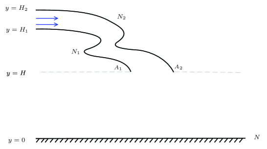
Figure 1. The nozzle walls and the ground

The resulting dynamics of the impinging jet is governed by the continuity equation and momentum equations in two dimensions,

$$\left\{\begin{array}[]{l}u_{x}+v_{y}=0,\\ uu_{x}+vu_{y}+p_{x}=0,\\ uv_{x}+vv_{y}+p_{y}=-g.\end{array}\right.$$ (1.1)

Here, $\displaystyle(u,v)$ is the velocity field, $\displaystyle p$ is the pressure of the incompressible fluid, and $\displaystyle g$ is the acceleration due to the gravity. The irrotational condition is written as

$$v_{x}-u_{y}=0.$$ (1.2)

The nozzle walls $\displaystyle N_{1}\cup N_{2}$ and the ground $\displaystyle N$ are assumed to be impermeable, and then the velocity satisfies the following no-flow condition,

$$(u,v)\cdot\vec{n}=0\ \ \text{on $\displaystyle N\cup N_{1}\cup N_{2}$},$$ (1.3)

where $\displaystyle\vec{n}$ is the outer normal to the boundaries.

In this paper, we will seek an impinging jet acted on by gravity and with two free streamlines, and the free streamlines initiate from the endpoints $\displaystyle A_{1}$ and $\displaystyle A_{2}$ of the nozzle, and extend to infinity.

Let $\displaystyle\Gamma_{1}$ and $\displaystyle\Gamma_{2}$ be the free streamlines connecting the nozzle walls $\displaystyle N_{1}$ and $\displaystyle N_{2}$, respectively. However, the location of the free streamlines is not known a priori. If the surface tension is negligible, the pressure on the free surface should be the constant atmospheric value $\displaystyle p_{atm}$. $\displaystyle\Omega_{0}$ denotes the flow region (which is unknown), bounded by the nozzle wall $\displaystyle N_{1}\cup N_{2}$, the free boundaries $\displaystyle\Gamma_{1}\cup\Gamma_{2}$ and the ground $\displaystyle N$ (see Figure 2).

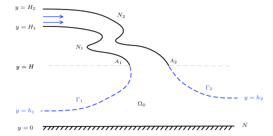
Figure 2. Impinging jet flow under gravity

Furthermore, the following notations will be used,

$$\text{$\displaystyle Q$~{}:~{}~{}the total incoming flux in upstream},$$ (1.4)

$$\text{$\displaystyle Q_{1}$~{}:~{}~{}the effluent flux in negative $\displaystyle x$-direction},$$

$$\text{$\displaystyle Q_{2}$~{}:~{}~{}the effluent flux in positive $\displaystyle x$-direction}.$$

It should be noted that the total incoming flux $\displaystyle Q=Q_{1}+Q_{2}$ is imposed in our problem and the quantities $\displaystyle Q_{1}$ and $\displaystyle Q_{2}$ are unknown a priori, which can be determined by the solution itself.

Now the impinging jet flow problem can be reformulated as: For any given total mass flux $\displaystyle Q$, determine an incompressible flow $\displaystyle(u,v,p)$ with free streamlines $\displaystyle\Gamma_{1}$ and $\displaystyle\Gamma_{2}$ connecting smoothly at the endpoints $\displaystyle A_{1}$ and $\displaystyle A_{2}$, on which the pressure is the given atmospheric pressure $\displaystyle p_{atm}$.

More precisely, a solution to the incompressible impinging jet problem is defined as follows.

Definition 1.1.

(a solution to the impinging jet problem) A vector $\displaystyle(u,v,p,\Gamma_{1},\Gamma_{2})$ is called a solution to the impinging jet problem, provided that the following properties hold:

Property 1. The free streamlines $\displaystyle\Gamma_{1}$ and $\displaystyle\Gamma_{2}$ can be described by $\displaystyle C^{1}$-smooth functions $\displaystyle x=k_{1}(y)$ and $\displaystyle x=k_{2}(y)$, respectively, and there exist two constants $\displaystyle h_{1},h_{2}\in(0,H)$, such that

$$\lim_{y\rightarrow h_{1}^{+}}k_{1}(y)=-\infty\ \ \text{and}\ \ \lim_{y\rightarrow h_{2}^{+}}k_{2}(y)=+\infty.$$

Property 2. The free boundaries $\displaystyle\Gamma_{1}$ and $\displaystyle\Gamma_{2}$ are analytic, and satisfy

$$g_{1}(H)=k_{1}(H)=-1\ \ \text{and}\ \ g_{2}(H)=k_{2}(H)=1,\$$ (1.5)

and

$$g^{\prime}_{1}(H+0)=k^{\prime}_{1}(H-0)\ \ \text{and}\ \ g^{\prime}_{2}(H+0)=k^{\prime}_{2}(H-0).$$ (1.6)

Property 3. $\displaystyle(u,v,p)\in\left(C^{1,\alpha}(\Omega_{0})\cap C^{0}(\overline{\Omega}_{0})\right)^{3}$ solves the steady incompressible Euler system (1.1), the irrotational condition (1.2) and the boundary condition (1.3).

Property 4. $\displaystyle p=p_{atm}$ on $\displaystyle\Gamma_{1}$ and $\displaystyle\Gamma_{2}$.

Remark 1.1.

The constants $\displaystyle h_{1}$ and $\displaystyle h_{2}$ are indeed the asymptotic widths of the impinging jet in left and right downstream, respectively. The property 1 in Definition 1.1 implies that the free boundaries $\displaystyle\Gamma_{1}$ and $\displaystyle\Gamma_{2}$ can not oscillate in downstream.

Remark 1.2.

The conditions (1.5) and (1.6) are so-called continuous fit conditions and smooth fit conditions for the impinging jet, which mean that the free boundaries connect the nozzle walls smoothly.

Remark 1.3.

The constant atmosphere pressure $\displaystyle p_{atm}$ is imposed arbitrarily in advance.

1.3. Main results

The main results of this paper are stated as follows. The first one is on the existence.

Theorem 1.1.

For any given atmosphere pressure $\displaystyle p_{atm}$ and total incoming flux $\displaystyle Q>2\sqrt{gH^{3}}$, there exists a solution $\displaystyle(u,v,p,\Gamma_{1},\Gamma_{2})$ to the incompressible impinging jet problem with gravity. Furthermore,
(1) the vertical velocity of the impinging jet is negative, namely, $\displaystyle v<0$ in $\displaystyle\Omega_{0}\cup\Gamma_{1}\cup\Gamma_{2}$.
(2) there exists a unique smooth streamline $\displaystyle\Gamma:x=k(y)$, which separates the impinging jet with two different downstream, and $\displaystyle\Gamma$ goes to the inlet of the nozzle and intersects the ground $\displaystyle N$ at the unique point $\displaystyle S$ (see Figure 3).
(3) The streamline $\displaystyle\Gamma$ is perpendicular to the ground $\displaystyle N$ at $\displaystyle S$, namely, $\displaystyle k^{\prime}(0+0)=0$.

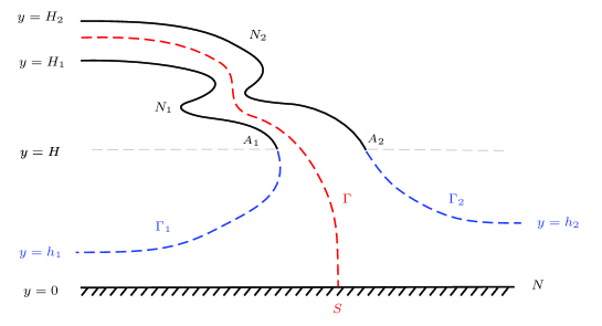
Figure 3. The interface $\displaystyle\Gamma$

Next, we will give the asymptotic behavior of the incompressible impinging jet under gravity.

Theorem 1.2.

Assume that there exists a large $\displaystyle R_{0}>1$, such that the nozzle wall $\displaystyle N_{i}$ can be described by $\displaystyle y=g_{i}^{-1}(x)$ for $\displaystyle x<-R_{0}$, $\displaystyle i=1,2$, then the impinging jet flow obtained in Theorem 1.1 satisfies the following asymptotic behavior in downstream,

$$\left(u,v,p\right)\rightarrow\left(-\frac{Q_{1}}{h_{1}},0,p_{1}(y)\right),\ \nabla(u,v)\rightarrow 0\ \text{and}\ \ \nabla p\rightarrow\left(0,-g\right)$$ (1.7)

uniformly in any compact subset of $\displaystyle(0,h_{1})$ as $\displaystyle x\rightarrow-\infty$, and

$$\left(u,v,p\right)\rightarrow\left(\frac{Q-Q_{1}}{h_{2}},0,p_{2}(y)\right),\ \nabla(u,v)\rightarrow 0\ \text{and}\ \ \nabla p\rightarrow\left(0,-g\right)$$ (1.8)

uniformly in any compact subset of $\displaystyle(0,h_{2})$ as $\displaystyle x\rightarrow+\infty$, where $\displaystyle Q_{1}$ is determined uniquely by

$$\frac{Q_{1}^{2}}{h_{1}^{2}}+2gh_{1}=\frac{(Q-Q_{1})^{2}}{h_{2}^{2}}+2gh_{2},$$

$\displaystyle p_{1}(y)=p_{atm}+g(h_{1}-y)$ for $\displaystyle y\in(0,h_{1})$ and $\displaystyle p_{2}(y)=p_{atm}+g(h_{2}-y)$ for $\displaystyle y\in(0,h_{2})$.

Similarly, in upstream,

$$\left(u,v,p\right)\rightarrow\left(\frac{Q}{H_{2}-H_{1}},0,p_{0}(y)\right),\ \nabla(u,v)\rightarrow 0\ \text{and}\ \ \nabla p\rightarrow\left(0,-g\right)$$ (1.9)

uniformly in any compact subset of $\displaystyle(H_{1},H_{2})$ as $\displaystyle x\rightarrow-\infty$, where $\displaystyle p_{0}(y)=p_{atm}+g(h_{1}-y)+\frac{Q_{1}^{2}}{2h_{1}^{2}}-\frac{Q^{2}}{2(H_{1}-H_{2})^{2}}$ for $\displaystyle y\in(H_{1},H_{2})$.

We would like to give some comments on the results as follows.

Remark 1.4.

In the significant work [3], the authors showed that in general there does not exist an asymmetric jet in gravity field issuing from a nozzle with infinite height, which satisfies the continuous fit conditions. However, the semi-infinite channel considered here possesses finite height, which seems physically reasonable and yet does not fall into the class studied in [3]. We establish the existence of the incompressible asymmetric impinging jet with continuous fit conditions under gravity for this class nozzles. This is the one of main differences to the work [3]. Meanwhile, ideas developed in this paper may provide a different way to establish the well-posedness of asymmetric jet flows under gravity without the horizontal plate $\displaystyle N$, by taking the limit $\displaystyle H\rightarrow+\infty$. This will be considered in the future.

Remark 1.5.

The mechanical behavior of the jet near the orifice is quite complicated because the flow has to adjust from a distribution compatible with the flow in a nozzle to the flow in a jet. Here we use the continuous and smooth fit conditions near the orifice, which is physically acceptable in the sense of Brillouin in [8] that the detachment is smooth at the fixed detached point. Yet, to ensure that such conditions are fulfilled mathematically is one of key elements to establish the existence of the impinging jet flow in this paper. The main new ideas are as follows. First, due to the Bernoulli’s law, the constant pressure condition on the free streamlines implies that

$$\frac{1}{2}(u^{2}+v^{2})+gy=constant\ \ \text{on}\ \ \Gamma_{1}\cup\Gamma_{2},$$

and this constant, denoted as $\displaystyle\lambda$ is undetermined at the present stage. On the other hand, as pointed out before, the effluent flux $\displaystyle Q_{1}$ is also not imposed here. Thus, to solve the impinging jet problem, we can treat the two quantities $\displaystyle(\lambda,Q_{1})$ as a pair of free parameters which will be adjusted to guarantee the continuous and smooth fit conditions. This is also the main difference from the problem of free jets without solid nozzle walls. It should be also mentioned that there are literatures on numerical and analytical results on the free jets of ideal fluids, see [9, 17, 25] and the references therein.

Remark 1.6.

Recall that in the absence of gravity, the existence of an impinging jet with two asymptotic directions and non-existence of an impinging jet with only one asymptotic direction have been shown in [10]. However, in this paper, our proof still excludes the critical cases $\displaystyle Q_{1}=0$ and $\displaystyle Q_{1}=Q$ and shows that $\displaystyle Q_{1}\in(0,Q)$ is the sufficient condition to the existence of impinging jet under gravity. This coincides with the results on impinging jets without gravity.

Remark 1.7.

One of the main differences between the impinging jets in [2, 3, 4] and general jets is the occurrence of the interface between the two fluids with different downstream. Here, we have to show the existence of the interface, and the uniqueness of the intersection point of the interface and the ground. In fact, we will show that the intersection point is a unique stagnation point in the fluid domain, furthermore, the interface $\displaystyle\Gamma$ intersects the ground perpendicularly at the stagnation point $\displaystyle S$ in Proposition 5.1.

Remark 1.8.

It should be noted that the assumption $\displaystyle Q>2\sqrt{gH^{3}}$ in Theorem 1.1 is a sufficient condition to exclude the stagnation point in the fluid domain (see Remark 2.1), especially on the free boundary. The advantage of this fact lies in exclusion the possible singularity on the free boundary of water waves with gravity. The singularity of the free surface flows with gravity at the stagnation point has been studied extensively in the elegant works [6, 22, 24, 26, 27, 28], which is closely related to a very interesting problem, the so-called Stokes Conjecture (Stokes [23] conjectured in 1880 that, at any stagnation point the free surface has a symmetric corner of $\displaystyle\frac{2\pi}{3}$). Therefore, unlike the results in [3], we do not restrict the deflection angle of the nozzle wall at the endpoints in this paper.

The remainder of this paper is organized as follows. Section 2 describes the set-up of the physical problem and formulates a free boundary problem for the stream function with two parameters $\displaystyle(\lambda,Q_{1})$. The solvability of the free boundary problem for any parameters follows from the standard variational approach in Section 2. To verify the continuous fit and smooth fit conditions, we will show that there exists a pair of parameters $\displaystyle(\lambda,Q_{1})$, such that the desired conditions hold in Section 3. We give the asymptotic behavior of the impinging jet in Section 4. Finally, we will investigate the existence, regularity and the properties of the interface $\displaystyle\Gamma$ and the branching point $\displaystyle S$ in Section 5.

2. Mathematical formulation of the impinging flow problem

In this section, we will formulate a boundary value problem with free boundaries, and furthermore, solve the free boundary problem by the variational method developed by Alt, Caffarelli and Friedman in [1, 2, 3]. For convenience to the readers, we will sketch the details and point out the differences as follows.

2.1. A free boundary problem

Due to the continuity equation, there exists a stream function $\displaystyle\psi(x,y)$, such that

$$\frac{\partial\psi}{\partial y}=u\ \ \text{and}\ \ \frac{\partial\psi}{\partial x}=-v.$$ (2.1)

The slip boundary conditions on the nozzle walls and the free boundaries imply that $\displaystyle N_{1}\cup\Gamma_{1}$ and $\displaystyle N_{2}\cup\Gamma_{2}$ are level sets of the stream function, and then without loss of generality, one assumes that

$$\psi=0\ \ \text{on}\ \ N_{1}\cup\Gamma_{1},\ \psi=Q_{1}\ \ \text{on}\ \ N\ \ \text{and}\ \psi=Q\ \ \ \text{on}\ \ \ N_{2}\cup\Gamma_{2}.$$

As mentioned before, in this work, we will seek an impinging jet under gravity with negative vertical velocity, and then it is reasonable to consider the free boundaries below the horizontal line $\displaystyle y=H$. Hence, we may assume that the possible fluid region is contained in the domain $\displaystyle\Omega$, bounded by $\displaystyle N_{1},N_{2},L_{1},L_{2}$ and $\displaystyle N$, where

$$L_{1}=\{(x,H)\mid x\leq-1\}\ \ \text{and}\ \ L_{2}=\{(x,H)\mid x\geq 1\}.$$

Moreover, we can define the free streamlines $\displaystyle\Gamma_{1}$ and $\displaystyle\Gamma_{2}$ as

$$\Gamma_{1}=\{0<y<H\}\cap\partial\{\psi>0\}\ \ \text{and}\ \ \Gamma_{2}=\{0<y<H\}\cap\partial\{\psi<Q\},$$ (2.2)

and the interface $\displaystyle\Gamma$ as

$$\Gamma=\Omega\cap\{\psi=Q_{1}\}.$$

Thus, the fluid region $\displaystyle\Omega_{0}=\Omega\cap\{0<\psi<Q\}$.

The irrotational condition implies

$$\Delta\psi=0\ \ \text{in}\ \ \Omega\cap\{0<\psi<Q\},$$

and the Bernoulli’s law gives that

$$\frac{|\nabla\psi|^{2}}{2}+gy+p=\text{constant}\ \ \text{in}\ \ \Omega\cap\{0<\psi<Q\}.$$ (2.3)

This, together with the constant pressure condition on the free streamlines, implies that $\displaystyle\frac{|\nabla\psi|^{2}}{2}+gy$ remains a constant on $\displaystyle\Gamma_{1}\cup\Gamma_{2}$, we denote this constant as $\displaystyle\lambda$. Hence, we formulate the following free boundary value problem in terms of a stream function.

$$\left\{\begin{array}[]{ll}&\Delta\psi=0\ \text{in}~{}~{}\Omega\cap\{0<\psi<Q\},\\ &\frac{\partial\psi}{\partial\nu}=-\sqrt{2\lambda-2gy}\ \ \text{on}~{}~{}\Gamma_{1},\ \frac{\partial\psi}{\partial\nu}=\sqrt{2\lambda-2gy}\ \ \text{on}~{}~{}\Gamma_{2},\\ &\psi=0\ \text{on}\ N_{1}\cup\Gamma_{1},\ \psi=Q\ \text{on}\ N_{2}\cup\Gamma_{2},\ \ \psi=Q_{1}\ \text{on}\ N,\end{array}\right.$$ (2.4)

where $\displaystyle\nu$ is the outer normal to the free boundaries.

The problem is now to find a stream function $\displaystyle\psi(x,y)$ solving the free boundary problem (2.4) with the continuous fit and smooth fit conditions. It should be emphasized that there are two undetermined parameters $\displaystyle\lambda$ and $\displaystyle Q_{1}$ in the free boundary problem, which will be determined by continuous fit conditions. In other words, we will solve the free boundary problem for any $\displaystyle\lambda$ and $\displaystyle Q_{1}$ first, and then show the existence of a pair of parameters $\displaystyle(\lambda,Q_{1})$ to guarantee the continuous fit conditions.

Once the free boundary problem (2.4) has been solved, the velocity field is given by (2.1) and the pressure is given by Bernoulli’s law, and then the free boundaries $\displaystyle\Gamma_{1}$ and $\displaystyle\Gamma_{2}$ are determined by (2.2).

2.2. On the asymptotic widths

In this subsection, we will find the relationship between the parameters $\displaystyle(\lambda,Q_{1})$ and the asymptotic widths $\displaystyle h_{1}$ and $\displaystyle h_{2}$ of the impinging jet in downstream if it exists.

Proposition 2.1.

For any given $\displaystyle Q>2\sqrt{gH^{3}}$,

(1) the parameters $\displaystyle\lambda>0$ and $\displaystyle Q_{1}\in[0,Q]$ can be determined uniquely by the asymptotic heights $\displaystyle h_{1}\in[0,H]$ and $\displaystyle h_{2}\in[0,H]$.

(2) for any given $\displaystyle Q_{1}\in(0,Q)$ and $\displaystyle\lambda\geq\frac{\max\{Q_{1}^{2},(Q-Q_{1})^{2}\}}{2H^{2}}+gH$, there exists a unique pair of asymptotic heights ($\displaystyle h_{1},h_{2}$) of the impinging jet flow with $\displaystyle h_{1}\in(0,H]$ and $\displaystyle h_{2}\in(0,H]$. Furthermore, $\displaystyle h_{1}$ increases with respect to $\displaystyle Q_{1}$ while $\displaystyle h_{2}$ decreases with respect to $\displaystyle Q_{1}$.

Proof.

(1). It is clear that

$$\text{$\displaystyle Q_{1}=\sqrt{2\lambda-2gh_{1}}h_{1}$ and $\displaystyle Q-Q_{1}=\sqrt{2\lambda-2gh_{2}}h_{2}$}.$$ (2.5)

Case 1. $\displaystyle h_{1}=h_{2}>0$, one has

$$Q_{1}=\frac{Q}{2}\ \ \text{and}\ \ \lambda=\frac{Q^{2}}{8h_{1}^{2}}+gh_{1}=\frac{Q^{2}}{8h_{2}^{2}}+gh_{2}.$$

Case 2. $\displaystyle h_{1}h_{2}=0$, one has

$$Q_{1}=0\ \ \text{and}\ \ \lambda=\frac{Q^{2}}{2h_{2}^{2}}+gh_{2}\ \ \text{for}\ \ h_{1}=0,$$

and

$$Q_{1}=Q\ \ \text{and}\ \ \lambda=\frac{Q^{2}}{2h_{1}^{2}}+gh_{1}\ \ \text{for}\ \ h_{2}=0.$$

Case 3. $\displaystyle h_{1}\neq h_{2}$ and $\displaystyle h_{1}h_{2}>0$, it follows from (2.5) that

$$Q_{1}^{2}=2\lambda h_{1}^{2}-2gh_{1}^{3}\ \ \text{and}\ \ (Q-Q_{1})^{2}=2\lambda h_{2}^{2}-2gh_{2}^{3},$$

which implies that

$$(h_{2}^{2}-h_{1}^{2})Q_{1}^{2}+2h_{1}^{2}QQ_{1}-(h_{1}^{2}Q^{2}+2gh_{1}^{2}h_{2}^{2}(h_{2}-h_{1}))=0.$$

Then we have

$$Q_{1}=\frac{-Qh_{1}^{2}+\sqrt{Q^{2}+2g(h_{2}^{2}-h_{1}^{2})(h_{2}-h_{1})}h_{1}h_{2}}{h_{2}^{2}-h_{1}^{2}},$$ (2.6)

or

$$Q_{1}=\frac{-Qh_{1}^{2}-\sqrt{Q^{2}+2g(h_{2}^{2}-h_{1}^{2})(h_{2}-h_{1})}h_{1}h_{2}}{h_{2}^{2}-h_{1}^{2}}\left\{\begin{array}[]{ll}<0,&\text{if}\ \ h_{1}<h_{2},\\ >Q,&\text{if}\ \ h_{1}>h_{2},\end{array}\right.$$

which can be dropped. It should be noted that

$$\sqrt{Q^{2}+2g(h_{2}^{2}-h_{1}^{2})(h_{2}-h_{1})}>Q\ \ \text{for any $\displaystyle h_{1}\neq h_{2}$}.$$

It suffices to show that $\displaystyle Q_{1}$ described in the formula (2.6) lies in $\displaystyle[0,Q]$. In fact, a direct calculation gives that

$$\begin{array}[]{rl}Q_{1}=\frac{h_{1}(Q^{2}+2g(h_{2}-h_{1})h_{2}^{2})}{Qh_{1}+\sqrt{Q^{2}+2g(h_{2}^{2}-h_{1}^{2})(h_{2}-h_{1})}h_{2}}.\end{array}$$

and

$$\begin{array}[]{rl}Q_{1}-Q=&\frac{-Qh_{2}^{2}+\sqrt{Q^{2}+2g(h_{2}^{2}-h_{1}^{2})(h_{2}-h_{1})}h_{1}h_{2}}{h_{2}^{2}-h_{1}^{2}}\\ =&\frac{h_{2}(-Q^{2}+2g(h_{2}-h_{1})h_{1}^{2})}{Qh_{2}+\sqrt{Q^{2}+2g(h_{2}^{2}-h_{1}^{2})(h_{2}-h_{1})}h_{1}}.\end{array}$$

Noting that $\displaystyle Q_{1}\geq 0$ and $\displaystyle Q_{1}-Q\leq 0$, due to the condition $\displaystyle Q>2\sqrt{gH^{3}}$.

Hence, $\displaystyle Q_{1}\in[0,Q]$ can be uniquely determined by $\displaystyle h_{1}$ and $\displaystyle h_{2}$. Furthermore, $\displaystyle\lambda=\frac{Q_{1}^{2}}{2h_{1}^{2}}+gh_{1}$ can be uniquely determined by $\displaystyle h_{1}$ and $\displaystyle Q_{1}$.

(2). Since $\displaystyle Q>2\sqrt{gH^{3}}$, we have $\displaystyle Q_{1}>\sqrt{gH^{3}}$ or $\displaystyle Q-Q_{1}>\sqrt{gH^{3}}$. Without loss of generality, we assume that $\displaystyle Q_{1}>\sqrt{gH^{3}}$.

Recall that $\displaystyle\lambda=\frac{Q_{1}^{2}}{2h_{1}^{2}}+gh_{1}=\frac{(Q-Q_{1})^{2}}{2h_{2}^{2}}+gh_{2}$. Set

$$\Lambda_{1}(t)=\frac{Q_{1}^{2}}{2t^{2}}+gt\ \ \text{and}\ \ \Lambda_{2}(t)=\frac{(Q-Q_{1})^{2}}{2t^{2}}+gt$$

for any fixed $\displaystyle Q_{1}\in[0,Q]$ and $\displaystyle t>0$. It is easy to check that

$$\Lambda^{\prime}_{1}(t)=\frac{gt^{3}-Q_{1}^{2}}{t^{3}}<0\ \ \text{for any $\displaystyle t\in(0,H]$}.$$ (2.7)

Since $\displaystyle\lambda\geq\frac{\max\{Q_{1}^{2},(Q-Q_{1})^{2}\}}{2H^{2}}+gH\geq\Lambda_{1}(H)$, it follows from (2.7) that $\displaystyle h_{1}\in(0,H]$ is determined uniquely by $\displaystyle\lambda$ and $\displaystyle Q_{1}$.

Similarly, we have

$$\Lambda_{2}^{\prime}(t)=-\frac{(Q-Q_{1})^{2}}{t^{3}}+g \Lambda_{2}^{\prime\prime}(t)=\frac{3(Q-Q_{1})^{2}}{t^{4}}>0 t>0$$ and for any .

Set $\displaystyle t_{0}=\frac{(Q-Q_{1})^{\frac{2}{3}}}{g^{\frac{1}{3}}}$, such that $\displaystyle\Lambda_{2}^{\prime}(t_{0})=0$. Then we consider the following two cases.

Case 1. $\displaystyle t_{0}\geq H$ (see Figure 4).

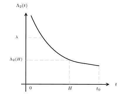
Figure 4. The relation $\displaystyle\Lambda_{2}(t)$ and $\displaystyle t$

Then $\displaystyle\Lambda_{2}^{\prime}(t)<0$ for any $\displaystyle t\in(0,H]$. On another side, the fact $\displaystyle\lambda\geq\frac{\max\{Q_{1}^{2},(Q-Q_{1})^{2}\}}{2H^{2}}+gH\geq\Lambda_{2}(H)$ implies that $\displaystyle h_{2}\in(0,H]$ can be determined uniquely by $\displaystyle\lambda=\frac{(Q-Q_{1})^{2}}{2h_{2}^{2}}+gh_{2}$.

Case 2. $\displaystyle t_{0}<H$ (see Figure 5), which is equivalent to $\displaystyle Q-Q_{1}<\sqrt{gH^{3}}$. This together with $\displaystyle Q_{1}>\sqrt{gH^{3}}$ gives that

$$\Lambda_{2}(H)=\frac{(Q-Q_{1})^{2}}{2H^{2}}+gH<\frac{Q_{1}^{2}}{2H^{2}}+gH\leq\lambda,$$

which implies that $\displaystyle h_{2}\in(0,H]$ is determined uniquely by $\displaystyle\lambda$ and $\displaystyle Q_{1}$, namely, $\displaystyle\lambda=\frac{(Q-Q_{1})^{2}}{2h_{2}^{2}}+gh_{2}$,

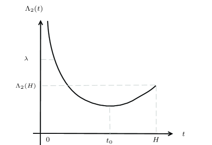
Figure 5. The relation $\displaystyle\Lambda_{2}(t)$ and $\displaystyle t$

Furthermore, we can conclude that $\displaystyle h_{1}$ is increasing with respect to $\displaystyle Q_{1}$ and $\displaystyle h_{2}$ is decreasing with respect to $\displaystyle Q_{1}$.

∎

Remark 2.1.

Note that $\displaystyle\lambda=\frac{Q_{1}^{2}}{2h_{1}^{2}}+gh_{1}=\frac{(Q-Q_{1})^{2}}{2h_{2}^{2}}+gh_{2}$. It follows from the proof of Proposition 2.1 that the condition $\displaystyle Q>2\sqrt{gH^{3}}$ ensures that one can choose $\displaystyle\lambda$ depending on $\displaystyle h_{1}$ and $\displaystyle h_{2}$ monotonically provided that

$$\lambda\geq\frac{\max\{Q_{1}^{2},(Q-Q_{1})^{2}\}}{2H^{2}}+gH.$$

Clearly, the right hand side has the following lower bound

$$\frac{Q^{2}}{8H^{2}}+gH,$$

which excludes the stagnation point on the free boundary $\displaystyle\Gamma_{1}\cup\Gamma_{2}$.

In particularly, for any $\displaystyle(Q_{1},\lambda)\in[0,Q]\times\left[\frac{\max\{Q_{1}^{2},(Q-Q_{1})^{2}\}}{2H^{2}}+gH,+\infty\right)$, there exists a unique pair $\displaystyle(h_{1},h_{2})$, such that

$$\lambda=\frac{Q_{1}^{2}}{2h_{1}^{2}}+gh_{1}=\frac{(Q-Q_{1})^{2}}{2h_{2}^{2}}+gh_{2}.$$

2.3. The variational approach

To solve the boundary value problem (2.4), we will use the variational method, which was developed by Alt, Caffarelli and Friedman in [1, 2, 3] for two-dimensional asymmetric jets and jets under gravity.

Define a functional with a parameter $\displaystyle\lambda$ as follows,

$$J_{\lambda}(\psi)=\int_{\Omega}|\nabla\psi|^{2}+(2\lambda-2gy)\chi_{\{0<\psi<Q\}\cap D}dxdy,$$ (2.8)

where $\displaystyle\chi_{E}$ is the characteristic function of a set $\displaystyle E$ and $\displaystyle D=\{0<y<H\}$. Define an admissible set with a parameter $\displaystyle Q_{1}$,

$$\begin{array}[]{rl}K_{Q_{1}}=\{\psi\in H^{1}_{loc}(\mathbb{R}^{2})\mid&\psi=Q_{1}\ \text{below}\ N,\psi=Q\ \text{in the right of}\ N_{2}\cup L_{2},\\ &\psi=0\ \text{in the left of}\ N_{1}\cup L_{1}\}.\end{array}$$

However, noting that the functional $\displaystyle J_{\lambda}(\psi)=+\infty$ for any $\displaystyle\psi\in K_{Q_{1}}$, we will consider the variational problem in a truncated domain. For any $\displaystyle\mu>1$, denote

$$\text{$\displaystyle H_{1,\mu}=\max\{y\mid g_{1}(y)=-\mu\}$}\ \ \text{$\displaystyle H_{2,\mu}=\min\{y>H_{1,\mu}\mid g_{2}(y)=-\mu\}$},$$ (2.9)

$$\text{$\displaystyle N_{1,\mu}=\{(x,y)\mid x=g_{1}(y),H\leq y\leq H_{1,\mu}\}$},\ \ \text{$\displaystyle L_{1,\mu}=L_{1}\cap\{x\geq-\mu\}$},$$

$$\text{$\displaystyle N_{2,\mu}=\{(x,y)\mid x=g_{2}(y),H\leq y\leq H_{2,\mu}\}$},\ \ \text{$\displaystyle L_{2,\mu}=L_{2}\cap\{x\leq\mu\}$},$$

$$\text{$\displaystyle\sigma_{1,\mu}=\{x=-\mu,0\leq y\leq H\}$},\ \ \text{ $\displaystyle\sigma_{2,\mu}=\{x=\mu,0\leq y\leq H\}$},$$

$$\text{$\displaystyle N_{\mu}=N\cap\{-\mu\leq x\leq\mu\}$},\ \ \text{$\displaystyle\sigma_{\mu}=\{x=-\mu,H_{1,\mu}\leq y\leq H_{2,\mu}\}$},$$

and $\displaystyle\Omega_{\mu}$ is bounded by $\displaystyle N_{1,\mu},N_{2,\mu},L_{1,\mu},L_{2,\mu},\sigma_{\mu},\sigma_{1,\mu},\sigma_{2,\mu}$ and $\displaystyle N_{\mu}$ (see Figure 6).

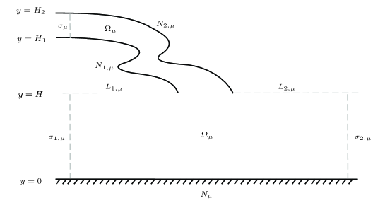
Figure 6. The truncated domain $\displaystyle\Omega_{\mu}$

Hence, one may consider the following truncated variational problem in the bounded domain $\displaystyle\Omega_{\mu}$. Define a functional

$$J_{\lambda,\mu}(\psi)=\int_{\Omega_{\mu}}|\nabla\psi|^{2}+(2\lambda-2gy)\chi_{\{0<\psi<Q\}\cap D_{\mu}}dxdy,$$

where $\displaystyle D_{\mu}=\{-\mu<x<\mu,0<y<H\}$.

The truncated variational problem $\displaystyle(P_{\lambda,Q_{1},\mu})$: For any $\displaystyle\mu>1$, $\displaystyle Q_{1}\in[0,Q]$ and $\displaystyle\lambda\geq\frac{\max\{Q_{1}^{2},(Q-Q_{1})^{2}\}}{2H^{2}}+gH$, find a $\displaystyle\psi_{\lambda,Q_{1},\mu}\in K_{\lambda,Q_{1},\mu}$, such that

$$\ \ \ J_{\lambda,\mu}(\psi_{\lambda,Q_{1},\mu})=\min_{\psi\in K_{\lambda,Q_{1},\mu}}J_{\lambda,\mu}(\psi),$$

where the admissible set $\displaystyle K_{\lambda,Q_{1},\mu}=\{\psi\in K_{Q_{1}}\mid\psi=\Psi_{\lambda,Q_{1},\mu}(x,y)\ \text{on}\ \partial\Omega_{\mu}\}$ and the boundary function

$$\Psi_{\lambda,Q_{1},\mu}(x,y)=\left\{\begin{array}[]{ll}0,&\text{on}\ \ N_{1,\mu}\cup L_{1,\mu},\\ Q,&\text{on}\ \ N_{2,\mu}\cup L_{2,\mu},\\ Q_{1},&\text{on}\ \ N_{\mu},\\ \max\left\{-\sqrt{2\lambda-2gh_{1}}y+Q_{1},0\right\},&\text{on}\ \ \sigma_{1,\mu},\\ \min\left\{\sqrt{2\lambda-2gh_{2}}y+Q_{1},Q\right\},&\text{on}\ \ \sigma_{2,\mu},\\ \frac{(y-H_{1,\mu})Q}{H_{2,\mu}-H_{1,\mu}}&\text{on}\ \ \sigma_{\mu}.\end{array}\right.$$

Here, $\displaystyle h_{1}$ and $\displaystyle h_{2}$ are the asymptotic heights of the impinging jets in left and right downstream, depending uniquely on $\displaystyle\lambda$ and $\displaystyle Q_{1}$ as in (2.5).

The existence of a minimizer $\displaystyle\psi_{\lambda,Q_{1},\mu}$ follows directly from Theorem 1.3 in [1], so the details are omitted here.

The corresponding free boundaries $\displaystyle\Gamma_{1,\lambda,Q_{1},\mu}$ and $\displaystyle\Gamma_{2,\lambda,Q_{1},\mu}$ are defined as

$$\text{$\displaystyle\Gamma_{1,\lambda,Q_{1},\mu}=D_{\mu}\cap\partial\{\psi_{\lambda,Q_{1},\mu}>0\}$ and $\displaystyle\Gamma_{2,\lambda,Q_{1},\mu}=D_{\mu}\cap\partial\{\psi_{\lambda,Q_{1},\mu}<Q\}$}.$$

It follows from Lemma 1.3, Lemma 2.3 and Lemma 2.4 in [1] that the following properties hold for the minimizer.

Proposition 2.2.

The minimizer $\displaystyle\psi_{\lambda,Q_{1},\mu}$ satisfies that

(1) $\displaystyle\psi_{\lambda,Q_{1},\mu}\in C^{0,1}(\Omega_{\mu})$ and is harmonic in $\displaystyle\Omega_{\mu}\cap\{0<\psi_{\lambda,Q_{1},\mu}<Q\}$.

(2) $\displaystyle 0\leq\psi_{\lambda,Q_{1},\mu}\leq Q$ in $\displaystyle\Omega_{\mu}$ and $\displaystyle 0<\psi_{\lambda,Q_{1},\mu}<Q$ in $\displaystyle\Omega_{\mu}\cap\{y>H\}$.

(3) The free boundaries $\displaystyle\Gamma_{1,\lambda,Q_{1},\mu}$ and $\displaystyle\Gamma_{2,\lambda,Q_{1},\mu}$ are analytic.

(4) $\displaystyle|\nabla\psi_{\lambda,Q_{1},\mu}|=\sqrt{2\lambda-2gy}$ on $\displaystyle\Gamma_{1,\lambda,Q_{1},\mu}\cup\Gamma_{2,\lambda,Q_{1},\mu}$.

Next, we will give a uniform estimate to the gradient of the minimizer away from the endpoints of the nozzle. The proof follows from the similar arguments in Section 5 in [2] immediately, and then the details are omitted here.

Lemma 2.3.

The minimizer $\displaystyle\psi_{\lambda,Q_{1},\mu}$ is continuous in $\displaystyle\bar{\Omega}_{\mu}$, and for any $\displaystyle\delta>0$, if $\displaystyle X\in\bar{\Omega}_{\mu}$ with $\displaystyle|X-A_{1}|>\delta$ and $\displaystyle|X-A_{2}|>\delta$, then there exists a constant $\displaystyle C$ depending on $\displaystyle\delta$ and $\displaystyle\Omega_{\mu}$, such that

$$|D\psi_{\lambda,Q_{1},\mu}(X)|\leq C(\sqrt{\lambda}+Q).$$

Furthermore, for any domain $\displaystyle K\Subset\Omega_{\mu}$ containing a free boundary point, the Lipschitz coefficient of $\displaystyle\psi_{\lambda,Q_{1},\mu}$ in $\displaystyle K$ is estimated by $\displaystyle C\sqrt{\lambda}$, where the constant $\displaystyle C$ depends on $\displaystyle K$ and $\displaystyle\Omega_{\mu}$, independent of $\displaystyle Q$.

2.4. The properties of the minimizer and the free boundaries

Next, we will establish some important properties of the minimizer and the free boundaries, such as monotonicity, uniqueness and regularity. First, we consider the monotonicity of the minimizer with respect to $\displaystyle x$. To this end, we will give a priori bounds of the minimizer as follows.

Lemma 2.4.

The minimizer $\displaystyle\psi_{\lambda,Q_{1},\mu}$ to the truncated variational problem $\displaystyle(P_{\lambda,Q_{1},\mu})$ satisfies

$$\max\left\{-\sqrt{2\lambda-2gh_{1}}y+Q_{1},0\right\}\leq\psi_{\lambda,Q_{1},\mu}(x,y)\leq\min\left\{\sqrt{2\lambda-2gh_{2}}y+Q_{1},Q\right\}\ \text{in}\ D_{\mu},$$ (2.10)

and

$$\max\left\{\frac{(y-H_{1,\mu})Q}{H_{2,\mu}-H_{1,\mu}},0\right\}<\psi_{\lambda,Q_{1},\mu}(x,y)<Q\ \quad\text{in}\ \ \Omega_{\mu}\cap\{y>H\},$$ (2.11)

where $\displaystyle H_{1,\mu}$ and $\displaystyle H_{2,\mu}$ are defined in (2.9).

Remark 2.2.

The bound (2.10) gives that

$$0<-\sqrt{2\lambda-2gh_{1}}y+Q_{1}\leq\psi_{\lambda,Q_{1},\mu}(x,y)\quad\quad\text{for}\quad y<h_{1},$$

and

$$\psi_{\lambda,Q_{1},\mu}(x,y)\leq\sqrt{2\lambda-2gh_{2}}y+Q_{1}<Q\quad\quad\text{for}\quad y<h_{2},$$

which in fact imply that the free boundary $\displaystyle\Gamma_{i,\lambda,Q_{1},\mu}$ lies above the asymptotic height $\displaystyle h_{i}$ for $\displaystyle i=1,2$. On another side, the bounds in (2.11) imply that the free boundaries lies below $\displaystyle y=H$.

Proof.

Consider the upper bound in (2.10) first. Since $\displaystyle\psi_{\lambda,Q_{1},\mu}\leq Q$ in $\displaystyle\Omega_{\mu}$, it suffices to obtain the upper bound in (2.10) for the case $\displaystyle Q_{1}<Q$.

Define an auxiliary comparison function

$$\omega_{\varepsilon}(y)=\min\left\{\sqrt{2\lambda-2g(h_{2}-\varepsilon)}y+Q_{1},Q\right\} \varepsilon\geq 0$$ for any ,

and a strip

$$D_{\mu,\varepsilon}=\Omega_{\mu}\cap\left\{y<\frac{Q-Q_{1}}{\sqrt{2\lambda-2g(h_{2}-\varepsilon)}}\right\}\ \ \text{for any $\displaystyle\varepsilon\geq 0$}.$$

Due to Lemma 2.3, $\displaystyle\psi_{\lambda,Q_{1},\mu}$ is Lipschitz continuous near $\displaystyle N_{\mu}$, this implies that there is a positive distance between the right free boundary and $\displaystyle N_{\mu}$. Thus, take a sufficiently large $\displaystyle\varepsilon>0$, such that

$$y=\frac{Q-Q_{1}}{\sqrt{2\lambda-2g(h_{2}-\varepsilon)}} \Gamma_{2,\lambda,Q_{1},\mu}$$ lies below the right free boundary .

It is easy to check that

$$\omega_{\varepsilon}>\psi_{\lambda,Q_{1},\mu} \sigma_{1,\mu}\cup\sigma_{2,\mu}$$  on

for any $\displaystyle\varepsilon\geq 0$, and it follows from Proposition 2.2 that

$$\psi_{\lambda,Q_{1},\mu}\leq Q=\omega_{\varepsilon}\ \ y=\frac{Q-Q_{1}}{\sqrt{2\lambda-2g(h_{2}-\varepsilon)}}$$  on ,

for $\displaystyle Q_{1}<Q$. If $\displaystyle\varepsilon$ is sufficiently large, $\displaystyle\psi_{\lambda,Q_{1},\mu}$ and $\displaystyle\omega_{\varepsilon}$ are harmonic in $\displaystyle D_{\mu,\varepsilon}$. Applying the maximum principle in $\displaystyle D_{\mu,\varepsilon}$ gives that

$$\psi_{\lambda,Q_{1},\mu}<\omega_{\varepsilon} D_{\mu,\varepsilon}$$ in ,

provided that $\displaystyle\varepsilon$ is sufficiently large.

Let $\displaystyle\varepsilon_{0}\geq 0$ be the smallest one and $\displaystyle y_{0}=\frac{Q-Q_{1}}{\sqrt{2\lambda-2g(h_{2}-\varepsilon_{0})}}$ (see Figure 7), such that

$$\psi_{\lambda,Q_{1},\mu}(x,y)<\omega_{\varepsilon_{0}}(y)\ \ \text{in}\ \ D_{\mu,\varepsilon_{0}},\ \ \text{and}\ \ \omega_{\varepsilon_{0}}(y_{0})=\psi_{\lambda,Q_{1},\mu}(x_{0},y_{0})\ \ \text{for some $\displaystyle x_{0}\in(-\mu,\mu)$. }$$

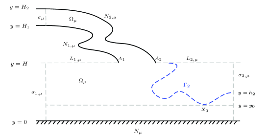
Figure 7. $\displaystyle\omega_{\varepsilon_{0}}$ and $\displaystyle\psi_{\lambda,Q_{1},\mu}$

It suffices to show that $\displaystyle\varepsilon_{0}=0$, and then the upper bound of the minimizer follows. If not, then $\displaystyle\varepsilon_{0}>0$, which implies that

$$y_{0}=\frac{Q-Q_{1}}{\sqrt{2\lambda-2g(h_{2}-\varepsilon_{0})}}<h_{2}.$$

Denote $\displaystyle X_{0}=(x_{0},y_{0})$. Since the free boundary $\displaystyle\Gamma_{2,\lambda,Q_{1},\mu}$ is analytic at $\displaystyle X_{0}$, it follows from Hopf’s lemma that

$$\sqrt{2\lambda-2gy_{0}}=\frac{\partial\psi_{\lambda,Q_{1},\mu}}{\partial\nu}>\frac{\partial\omega_{\varepsilon_{0}}}{\partial\nu}=\sqrt{2\lambda-2g(h_{2}-\varepsilon_{0})}=\frac{Q-Q_{1}}{y_{0}}=\frac{\sqrt{2\lambda-2gh_{2}}h_{2}}{y_{0}}\ \ \text{at}\ \ X_{0},$$

where $\displaystyle\nu=(0,1)$ is the outer normal vector to $\displaystyle\Gamma_{2,\lambda,Q_{1},\mu}$ at $\displaystyle X_{0}=(x_{0},y_{0})$. This is nothing but

$$y_{0}\sqrt{2\lambda-2gy_{0}}>h_{2}\sqrt{2\lambda-2gh_{2}}\ \ \text{for $\displaystyle y_{0}<h_{2}$}.$$ (2.12)

On another side, it is clear that the function $\displaystyle t\sqrt{2\lambda-2gt}$ is strictly increasing with respect to $\displaystyle t\in(0,H)$, which contradicts to (2.12).

Similarly, one can show that

$$\psi(x,y)\geq\max\left\{-\sqrt{2\lambda-2gh_{1}}y+Q_{1},0\right\}\ \ \text{in}\ \ D_{\mu}.$$

Finally, consider the estimate (2.11) in the nozzle. Denote $\displaystyle G_{\mu}=\Omega_{\mu}\cap\{y>H_{1,\mu}\}$. Applying the maximum principle in $\displaystyle G_{\mu}$ gives that $\displaystyle\frac{(y-H_{1,\mu})Q}{H_{2,\mu}-H_{1,\mu}}\leq\psi_{\lambda,Q_{1},\mu}$ in $\displaystyle G_{\mu}$. Since $\displaystyle 0<\psi_{\lambda,Q_{1},\mu}<Q$ in $\displaystyle\Omega_{\mu}\cap\{y>H\}$, it follows

$$\max\left\{\frac{(y-H_{1,\mu})Q}{H_{2,\mu}-H_{1,\mu}},0\right\}<\psi_{\lambda,Q_{1},\mu}(x,y)<Q\ \quad\quad\text{in}\ \ \Omega_{\mu}\cap\{y>H\}.$$

∎

With the aid of Lemma 2.4, one can obtain the uniqueness and monotonicity of the minimizer $\displaystyle\psi_{\lambda,Q_{1},\mu}$.

Proposition 2.5.

The minimizer $\displaystyle\psi_{\lambda,Q_{1},\mu}(x,y)$ to the truncated variational problem $\displaystyle(P_{\lambda,Q_{1},\mu})$ is increasing with respect to $\displaystyle x$. Furthermore, the minimizer $\displaystyle\psi_{\lambda,Q_{1},\mu}$ is unique for any fixed $\displaystyle\lambda,Q_{1}$ and $\displaystyle\mu$.

Proof.

Suppose that $\displaystyle\psi(x,y)=\psi_{\lambda,Q_{1},\mu}(x,y)$ and $\displaystyle\tilde{\psi}(x,y)=\tilde{\psi}_{\lambda,Q_{1},\mu}(x,y)$ are two minimizers to the truncated variational problem $\displaystyle(P_{\lambda,Q_{1},\mu})$. Define $\displaystyle\tilde{\psi}_{\varepsilon}(x,y)=\tilde{\psi}(x-\varepsilon,y)$ for any $\displaystyle\varepsilon\geq 0$, the corresponding functional $\displaystyle J_{\lambda,\mu}^{\varepsilon}$ with admissible set $\displaystyle K_{\lambda,Q_{1},\mu}^{\varepsilon}$ in truncated domain $\displaystyle\Omega_{\mu}^{\varepsilon}=\{(x,y)\mid(x-\varepsilon,y)\in\Omega_{\mu}\}$. Extend $\displaystyle\psi(x,y)$ and $\displaystyle\tilde{\psi}_{\varepsilon}(x,y)$ to larger domain, respectively, as

$$\psi(x,y)=\min\left\{\sqrt{2\lambda-2gh_{2}}y+Q_{1},Q\right\} \mu\leq x\leq\mu+\varepsilon,0\leq y\leq H$$ for

and

$$\tilde{\psi}_{\varepsilon}(x,y)=\left\{\begin{array}[]{ll}\max\left\{-\sqrt{2\lambda-2gh_{1}}y+Q_{1},0\right\},&\text{for}\ -\mu\leq x\leq-\mu+\varepsilon,0\leq y\leq H,\\ \max\left\{\frac{(y-H_{1,\mu})Q}{H_{2,\mu}-H_{1,\mu}},0\right\},&\text{for}\ -\mu\leq x\leq-\mu+\varepsilon,H\leq y\leq H_{2,\mu}.\end{array}\right.$$

Set

$$\psi_{1}=\max\{\psi,\tilde{\psi}_{\varepsilon}\}\ \ \text{and}\ \ \psi_{2}=\min\{\psi,\tilde{\psi}_{\varepsilon}\}.$$

Then Lemma 2.4 gives that

$$\psi_{1}=\psi\ \ \text{in $\displaystyle\Omega_{\mu}^{\varepsilon}\setminus\Omega_{\mu}$ and }\ \psi_{2}=\tilde{\psi}_{\varepsilon}\ \ \text{in $\displaystyle\Omega_{\mu}\setminus\Omega_{\mu}^{\varepsilon}$},$$ (2.13)

which implies that $\displaystyle\psi_{1}\in K_{\lambda,Q_{1},\mu}$ and $\displaystyle\psi_{2}\in K_{\lambda,Q_{1},\mu}^{\varepsilon}$. Next, we claim that

$$J_{\lambda,\mu}(\psi)=J_{\lambda,\mu}(\psi_{1})\ \ \text{and}\ \ J_{\lambda,\mu}^{\varepsilon}(\tilde{\psi}_{\varepsilon})=J_{\lambda,\mu}^{\varepsilon}(\psi_{2}).$$ (2.14)

Indeed, since $\displaystyle J_{\lambda,\mu}(\psi)\leq J_{\lambda,\mu}(\psi_{1})$ and $\displaystyle J_{\lambda,\mu}^{\varepsilon}(\tilde{\psi}_{\varepsilon})\leq J_{\lambda,\mu}^{\varepsilon}(\psi_{2})$, (2.14) will follow from

$$J_{\lambda,\mu}(\psi)+J_{\lambda,\mu}^{\varepsilon}(\tilde{\psi}_{\varepsilon})=J_{\lambda,\mu}(\psi_{1})+J_{\lambda,\mu}^{\varepsilon}(\psi_{2}).$$ (2.15)

In fact, (2.13) implies that $\displaystyle\psi\geq\tilde{\psi}_{\varepsilon}$ in $\displaystyle(\Omega_{\mu}^{\varepsilon}\setminus\Omega_{\mu})\cup(\Omega_{\mu}\setminus\Omega_{\mu}^{\varepsilon})$. Therefore one has

$$\Omega_{\mu}\cap\{\psi<\tilde{\psi}_{\varepsilon}\}=\Omega_{\mu}^{\varepsilon}\cap\{\psi<\tilde{\psi}_{\varepsilon}\}.$$ (2.16)

Due to (2.16), one may get

$$\begin{array}[]{rl}&\int_{\Omega_{\mu}}|\nabla\psi_{1}|^{2}dxdy+\int_{\Omega_{\mu}^{\varepsilon}}|\nabla\psi_{2}|^{2}dxdy\\ =&\int_{\Omega_{\mu}\cap\{\psi\geq\tilde{\psi}_{\varepsilon}\}}|\nabla\psi|^{2}dxdy+\int_{\Omega_{\mu}\cap\{\psi<\tilde{\psi}_{\varepsilon}\}}|\nabla\tilde{\psi}_{\varepsilon}|^{2}dxdy\\ &+\int_{\Omega_{\mu}^{\varepsilon}\cap\{\psi\geq\tilde{\psi}_{\varepsilon}\}}|\nabla\tilde{\psi}_{\varepsilon}|^{2}dxdy+\int_{\Omega_{\mu}^{\varepsilon}\cap\{\psi<\tilde{\psi}_{\varepsilon}\}}|\nabla\psi|^{2}dxdy\\ =&\int_{\Omega_{\mu}\cap\{\psi\geq\tilde{\psi}_{\varepsilon}\}}|\nabla\psi|^{2}dxdy+\int_{\Omega_{\mu}^{\varepsilon}\cap\{\psi<\tilde{\psi}_{\varepsilon}\}}|\nabla\tilde{\psi}_{\varepsilon}|^{2}dxdy\\ &+\int_{\Omega_{\mu}^{\varepsilon}\cap\{\psi\geq\tilde{\psi}_{\varepsilon}\}}|\nabla\tilde{\psi}_{\varepsilon}|^{2}dxdy+\int_{\Omega_{\mu}\cap\{\psi<\tilde{\psi}_{\varepsilon}\}}|\nabla\psi|^{2}dxdy\\ =&\int_{\Omega_{\mu}}|\nabla\psi|^{2}dxdy+\int_{\Omega_{\mu}^{\varepsilon}}|\nabla\tilde{\psi}_{\varepsilon}|^{2}dxdy.\end{array}$$ (2.17)

Similarly, one has

$$\begin{array}[]{rl}&\int_{D_{\mu}}(2\lambda-2gy)\chi_{\{0<\psi<Q\}}dxdy+\int_{D_{\mu}^{\varepsilon}}(2\lambda-2gy)\chi_{\{0<\tilde{\psi}_{\varepsilon}<Q\}}dxdy\\ =&\int_{D_{\mu}}(2\lambda-2gy)\chi_{\{0<\psi_{1}<Q\}}dxdy+\int_{D_{\mu}^{\varepsilon}}(2\lambda-2gy)\chi_{\{0<\psi_{2}<Q\}}dxdy,\end{array}$$

which, together with (2.17), gives (2.15). And hence the claim (2.14) is proved.

Moreover, we will show that if $\displaystyle 0<\psi(X_{0})=\tilde{\psi}_{\varepsilon}(X_{0})<Q$ with $\displaystyle X_{0}\in\Omega_{\mu}\cap\Omega_{\mu}^{\varepsilon}$, then

either $$\psi\geq\tilde{\psi}_{\varepsilon} \psi\leq\tilde{\psi}_{\varepsilon} X_{0}$$ or  in some neighborhood of . (2.18)

By the continuity of $\displaystyle\psi$, $\displaystyle 0<\psi<Q$ in $\displaystyle B_{r}(X_{0})\subset\Omega_{\mu}\cap\Omega_{\mu}^{\varepsilon}$ for some small $\displaystyle r>0$. Define a function $\displaystyle\phi$ as follows,

$$\Delta\phi=0\ \ \text{in}\ \ B_{r}(X_{0})\ \ \text{and $\displaystyle\phi=\psi_{1}$ on $\displaystyle\partial B_{r}(X_{0})$}.$$ (2.19)

Suppose that (2.18) is not true, we then claim that $\displaystyle\psi_{1}$ is not harmonic in $\displaystyle B_{r}(X_{0})$ for any small $\displaystyle r>0$. In fact, if $\displaystyle\psi_{1}$ solves the boundary value problem (2.19), and it is easy to check that $\displaystyle\Delta\psi=0$ in $\displaystyle B_{r}(X_{0})$ and $\displaystyle\psi\leq\psi_{1}$ on $\displaystyle\partial B_{r}(X_{0})$, the strong maximum principle gives that $\displaystyle\psi\equiv\psi_{1}$ in $\displaystyle B_{r}(X_{0})$, due to $\displaystyle\psi(X_{0})=\psi_{1}(X_{0})$. Namely, $\displaystyle\psi\geq\tilde{\psi}_{\varepsilon}$ in $\displaystyle B_{r}(X_{0})$, which contradicts to our assumption.

Since $\displaystyle\psi_{1}$ is not harmonic in $\displaystyle B_{r}(X_{0})$, and $\displaystyle\psi_{1}\neq\phi$ in $\displaystyle B_{r}(X_{0})$. Then it holds that

$$\begin{array}[]{rl}&\int_{B_{r}(X_{0})}|\nabla\phi|^{2}dxdy-\int_{B_{r}(X_{0})}|\nabla\psi_{1}|^{2}dxdy\\ =&-\int_{B_{r}(X_{0})}|\nabla(\phi-\psi_{1})|^{2}dxdy+2\int_{B_{r}(X_{0})}\nabla\phi\cdot\nabla(\phi-\psi_{1})dxdy\\ =&-\int_{B_{r}(X_{0})}|\nabla(\phi-\psi_{1})|^{2}dxdy\\ <&0.\end{array}$$ (2.20)

Extend $\displaystyle\phi=\psi_{1}$ outside $\displaystyle B_{r}(X_{0})$, such that $\displaystyle\phi\in K_{\lambda,Q_{1},\mu}$. It follows from (2.20) and the fact that $\displaystyle 0<\phi<Q$ in $\displaystyle\overline{B_{r}(X_{0})}$ that

$$J_{\lambda,\mu}(\phi)<J_{\lambda,\mu}(\psi_{1})=J_{\lambda,\mu}(\psi),$$

which contradicts to the fact that $\displaystyle\psi$ is a minimizer to the variational problem $\displaystyle(P_{\lambda,Q_{1},\mu})$. Hence, the claim (2.18) is proved.

Next, we will show that

$$\text{$\displaystyle\Omega_{\mu}\cap\{0<\psi<Q\}$ and $\displaystyle\Omega_{\mu}^{\varepsilon}\cap\{0<\tilde{\psi}_{\varepsilon}<Q\}$ are connected}.$$ (2.21)

If (2.21) fails, then without loss of generality, we assume that $\displaystyle\Omega_{\mu}\cap\{0<\psi<Q\}$ is not connected. Since $\displaystyle 0<\psi<Q$ in $\displaystyle\Omega_{\mu}\cap\{y>H\}$ (see (2.11)), let $\displaystyle E$ be a maximal connected subset of $\displaystyle\Omega_{\mu}\cap\{0<\psi<Q\}$, such that $\displaystyle\Omega_{\mu}\cap\{y>H\}\subset E$. Then there exists a point $\displaystyle Y_{0}\in\Omega_{\mu}\cap\{0<\psi<Q\}$, such that $\displaystyle Y_{0}\notin E$. The continuity of $\displaystyle\psi$ gives that there exists a maximal connected subset $\displaystyle F$ in $\displaystyle\Omega_{\mu}\cap\{0<\psi<Q\}$ and $\displaystyle Y_{0}\in F$.

If $\displaystyle\partial\Omega_{\mu}\cap\partial F=\varnothing$, we first show that $\displaystyle\psi=0$ or $\displaystyle\psi=Q$ on $\displaystyle\partial F$. If not, there exists a point $\displaystyle X_{0}\in\partial F$ with $\displaystyle 0<\psi(X_{0})<Q$. Due to the continuity of $\displaystyle\psi$ again, there exists a connected subsect $\displaystyle\tilde{F}$ of $\displaystyle\Omega_{\mu}\cap\{0<\psi<Q\}$, such that $\displaystyle F\subseteq\tilde{F}$, which contradicts to the definition of the set $\displaystyle F$. Since $\displaystyle\psi$ is harmonic in $\displaystyle F$, the strong maximum principle gives that $\displaystyle\psi\equiv 0$ or $\displaystyle\psi\equiv Q$ in $\displaystyle F$, which contradicts to the fact $\displaystyle 0<\psi(Y_{0})<Q$ with $\displaystyle Y_{0}\in F$.

If $\displaystyle\partial\Omega_{\mu}\cap\partial F\neq\varnothing$, the definition of $\displaystyle F$ implies that $\displaystyle\psi\equiv 0$ or $\displaystyle\psi\equiv Q$ on $\displaystyle\Omega_{\mu}\cap\partial F$. Without loss of generality, one may assume that $\displaystyle\psi\equiv 0$ on $\displaystyle\Omega_{\mu}\cap\partial F$. Hence, $\displaystyle\psi\equiv 0$ on $\displaystyle\partial\Omega_{\mu}\cap\partial F$, since $\displaystyle\psi$ is continuous up to $\displaystyle\partial\Omega_{\mu}$ and is monotone with respect to $\displaystyle y$ on $\displaystyle\partial\Omega_{\mu}$. Therefore, $\displaystyle\psi\equiv 0$ on $\displaystyle\partial F$, which together with the strong maximum principle gives that $\displaystyle\psi\equiv 0$ in $\displaystyle F$. This is a contradiction to the definition of $\displaystyle F$.

Hence, the claim (2.21) is obtained.

By virtue of (2.18), one has that

$$\text{there does not exist some point $\displaystyle X_{0}\in\Omega_{\mu}$, such that $\displaystyle 0<\psi(X_{0})=\tilde{\psi}_{\varepsilon}(X_{0})<Q$}.$$ (2.22)

In fact, suppose that there exists a point $\displaystyle X_{0}=(x_{0},y_{0})\in\Omega_{\mu}$, such that $\displaystyle 0<\psi(X_{0})=\tilde{\psi}_{\varepsilon}(X_{0})<Q$. Then there are two cases to be considered.

Case 1. $\displaystyle X_{0}\in\Omega_{\mu}\cap\Omega_{\mu}^{\varepsilon}$. In view of the claim (2.18), we have that either $\displaystyle\psi\geq\tilde{\psi}_{\varepsilon}$ or $\displaystyle\psi\leq\tilde{\psi}_{\varepsilon}$ in $\displaystyle B_{r}(X_{0})\subset(\Omega_{\mu}\cap\{0<\psi<Q\})\cap(\Omega_{\mu}^{\varepsilon}\cap\{0<\tilde{\psi}_{\varepsilon}<Q\})$ for some small $\displaystyle r>0$. The strong maximum principle gives that $\displaystyle\psi\equiv\tilde{\psi}_{\varepsilon}$ in $\displaystyle B_{r}(X_{0})$, due to $\displaystyle\psi(X_{0})=\tilde{\psi}_{\varepsilon}(X_{0})$. By virtue of (2.21), applying strong maximum principle again, we can conclude that

$$\text{$\displaystyle\psi\equiv\tilde{\psi}_{\varepsilon}$ in $\displaystyle(\Omega_{\mu}\cap\{0<\psi<Q\})\cap(\Omega_{\mu}^{\varepsilon}\cap\{0<\tilde{\psi}_{\varepsilon}<Q\})$},$$

which leads to a contradiction to the fact that $\displaystyle\tilde{\psi}_{\varepsilon}<Q=\psi$ on $\displaystyle N_{2,\mu}$.

Case 2. $\displaystyle X_{0}\in\Omega_{\mu}\setminus\Omega_{\mu}^{\varepsilon}$. Then there are three subcases.

Subcase 2.1. $\displaystyle X_{0}\in(\Omega_{\mu}\setminus\Omega_{\mu}^{\varepsilon})\cap\{y>H_{1,\mu}\}$. The extension of $\displaystyle\tilde{\psi}_{\varepsilon}$ implies that $\displaystyle 0<\psi(X_{0})=\tilde{\psi}_{\varepsilon}(X_{0})=\frac{(y_{0}-H_{1,\mu})Q}{H_{2,\mu}-H_{1,\mu}}<Q,$ which contradicts to the lower bound in (2.11).

Subcase 2.2. $\displaystyle X_{0}\in(\Omega_{\mu}\setminus\Omega_{\mu}^{\varepsilon})\cap\{h_{1}\leq y\leq H_{1,\mu}\}$. It is easy to see that $\displaystyle\tilde{\psi}_{\varepsilon}(X_{0})=0$, which contradicts to our assumption $\displaystyle 0<\tilde{\psi}_{\varepsilon}(X_{0})<Q$.

Subcase 2.3. $\displaystyle X_{0}\in(\Omega_{\mu}\setminus\Omega_{\mu}^{\varepsilon})\cap\{y<h_{1}\}$. Noticing the extension of $\displaystyle\tilde{\psi}_{\varepsilon}$, one has that $\displaystyle 0<\psi(X_{0})=\tilde{\psi}_{\varepsilon}(X_{0})=-\sqrt{2\lambda-2gh_{1}}y_{0}+Q_{1}<Q.$ The continuity of $\displaystyle\psi$ gives that there exists a small $\displaystyle r>0$, such that $\displaystyle 0<\psi<Q$ in $\displaystyle B_{r}(X_{0})\subset\Omega_{\mu}$ and $\displaystyle y_{0}+r<h_{1}$. Due to the lower bound $\displaystyle\psi\geq-\sqrt{2\lambda-2gh_{1}}y+Q_{1}$ in (2.10), the strong maximum principle implies that $\displaystyle\psi(X_{0})\equiv-\sqrt{2\lambda-2gh_{1}}y_{0}+Q_{1}$ in $\displaystyle B_{r}(X_{0})$. In view of (2.21), by using the strong maximum principle again, one gets that $\displaystyle\psi(X_{0})\equiv-\sqrt{2\lambda-2gh_{1}}y_{0}+Q_{1}$ in $\displaystyle\Omega_{\mu}\cap\{y<h_{1}\}$, which leads to a contradiction to the boundary value of $\displaystyle\psi$ on $\displaystyle\sigma_{2,\mu}$.

Since $\displaystyle\tilde{\psi}_{\varepsilon}<Q=\psi$ on $\displaystyle N_{2,\mu}$, it follows from (2.21) and (2.22) that

$$\ \psi(x,y)\geq\tilde{\psi}(x-\varepsilon,y)\ \quad\quad\text{in $\displaystyle\Omega_{\mu}$}.$$ (2.23)

Similarly, one can obtain that

$$\ \psi(x,y)\leq\tilde{\psi}(x+\varepsilon,y)\ \quad\quad\text{in $\displaystyle\Omega_{\mu}$}.$$ (2.24)

Taking $\displaystyle\varepsilon\rightarrow 0$ in (2.23) and (2.24) implies that $\displaystyle\psi=\tilde{\psi}$.

In particular, taking $\displaystyle\psi=\tilde{\psi}$ in (2.23), we conclude that $\displaystyle\psi(x,y)$ is monotone increasing with respect to $\displaystyle x$.

∎

2.5. The free boundaries of the minimizer

Thanks to the monotonicity of $\displaystyle\psi_{\lambda,Q_{1},\mu}$ with respect to $\displaystyle x$ in Proposition 2.5, there exist two functions $\displaystyle k_{1,\lambda,Q_{1},\mu}(y)$ and $\displaystyle k_{2,\lambda,Q_{1},\mu}(y)$ such that

$$\begin{array}[]{rl}&D_{\mu}\cap\{0<\psi_{\lambda,Q_{1},\mu}<Q\}\\ =&\{(x,y)\in D_{\mu}\mid k_{1,\lambda,Q_{1},\mu}(y)<x<k_{2,\lambda,Q_{1},\mu}(y)\ \ \text{for}\ \ 0<y<H\}.\end{array}$$ (2.25)

In order to establish the continuity of free boundaries, we need the following non-oscillation lemma, which implies that the free boundary cannot oscillate near any free boundary point.

Lemma 2.6.

(non-oscillation lemma) Suppose that there exist some $\displaystyle\alpha_{1},\alpha_{2}$ with $\displaystyle\alpha_{1}<\alpha_{2}$ and a domain $\displaystyle E\subset D_{\mu}\cap\{0<\psi_{\lambda,Q_{1},\mu}<Q\}$, such that

(1) $\displaystyle E$ is bounded by two disjoint arcs $\displaystyle\gamma_{1},\gamma_{2}$ ($\displaystyle\gamma_{1},\gamma_{2}\subset\Gamma_{2,\lambda,Q_{1},\mu})$, the lines $\displaystyle\{x=\alpha_{1}\}$ and $\displaystyle\{x=\alpha_{2}\}$ (see Figure 8). Denote the endpoints of $\displaystyle\gamma_{i}$ as $\displaystyle(\alpha_{1},\beta_{i})$ and $\displaystyle(\alpha_{2},\eta_{i})$ for $\displaystyle i=1,2$.

(2) dist$\displaystyle(E,\overline{A_{1}A_{2}})>c_{0}$ for some $\displaystyle c_{0}>0$.

There exists a constant $\displaystyle C>0$, depending only on $\displaystyle\lambda,H,c_{0}$ and $\displaystyle Q$, such that

$$|\alpha_{2}-\alpha_{1}|\leq C\max\{|\beta_{1}-\beta_{2}|,|\eta_{1}-\eta_{2}|\}.$$

A similar result holds for $\displaystyle\gamma_{1},\gamma_{2}\subset\Gamma_{1,\lambda,Q_{1},\mu}$.

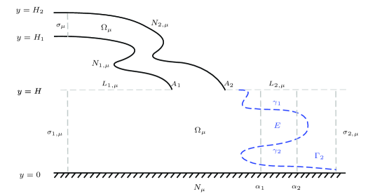
Figure 8. The domain $\displaystyle E$

Proof.

Denote $\displaystyle h=\max\left\{|\beta_{1}-\beta_{2}|,|\eta_{1}-\eta_{2}|\right\}$ and $\displaystyle\psi=\psi_{\lambda,Q_{1},\mu}$. Since $\displaystyle\psi$ is harmonic in $\displaystyle E$, it is easy to check that $\displaystyle\int_{\partial E}\frac{\partial\psi}{\partial\nu}dS=0$, which yields that

$$\int_{\gamma_{1}\cup\gamma_{2}}\sqrt{2\lambda-2gy}dS=\int_{\gamma_{1}\cup\gamma_{2}}\frac{\partial\psi}{\partial\nu}dS=-\int_{\partial E\cap\{x=\alpha_{2}\}}\frac{\partial\psi}{\partial x}dy+\int_{\partial E\cap\{x=\alpha_{1}\}}\frac{\partial\psi}{\partial x}dy,$$

where $\displaystyle\gamma_{1}$ and $\displaystyle\gamma_{2}$ are two arcs of the right free boundary.

By virtue of the Lipschitz continuity of $\displaystyle\psi$, one has

$$\begin{array}[]{rl}-\int_{\partial E\cap\{x=\alpha_{2}\}}\frac{\partial\psi}{\partial x}dy+\int_{\partial E\cap\{x=\alpha_{1}\}}\frac{\partial\psi}{\partial x}dy\leq Ch.\end{array}$$ (2.26)

On the other hand, one gets

$$\int_{\gamma_{1}\cup\gamma_{2}}\sqrt{2\lambda-2gy}dS\geq 2\sqrt{2\lambda-2gH}(\alpha_{2}-\alpha_{1}),$$

which together with (2.26) gives that

$$\alpha_{2}-\alpha_{1}\leq Ch.$$

∎

Remark 2.3.

The non-oscillation Lemma 2.6 remains true if one of the arcs, $\displaystyle\gamma_{1}$ for example, is a line segment (see Figure 9), and

$$\frac{\partial\psi_{\lambda,Q_{1},\mu}}{\partial\nu}\geq 0\ \ \text{on}\ \ \gamma_{1}.$$ (2.27)

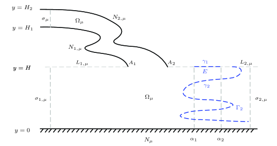
Figure 9. The domain $\displaystyle E$

With the aid of the non-oscillation Lemma 2.6, we can show the continuity of $\displaystyle k_{1,\lambda,Q_{1},\mu}(y)$ and $\displaystyle k_{2,\lambda,Q_{1},\mu}(y)$.

Lemma 2.7.

$\displaystyle k_{1,\lambda,Q_{1},\mu}(y)$ is continuous in $\displaystyle(h_{1},H)$ and $\displaystyle k_{2,\lambda,Q_{1},\mu}(y)$ is continuous in $\displaystyle(h_{2},H)$. Furthermore, $\displaystyle k_{i,\lambda,Q_{1},\mu}(H)=\lim_{y\rightarrow H^{-}}k_{i,\lambda,Q_{1},\mu}(y)$ exists for $\displaystyle i=1,2$.

Proof.

Denote $\displaystyle\psi=\psi_{\lambda,Q_{1},\mu}$ and $\displaystyle k_{i}(y)=k_{i,\lambda,Q_{1},\mu}(y)$ ($\displaystyle i=1,2$) for simplicity. We consider only the continuity of $\displaystyle k_{2}(y)$ in the following, and the continuity of $\displaystyle k_{1}(y)$ can be obtained by similar arguments.

As mentioned in Remark 2.2, the free boundary $\displaystyle\Gamma_{2,\lambda,Q_{1},\mu}$ lies above $\displaystyle y=h_{2}$. First, we will show that the one side limit of $\displaystyle k_{2}(y)$ exists as $\displaystyle y\rightarrow y_{0}^{-}$ or $\displaystyle y\rightarrow y_{0}^{+}$ for any $\displaystyle y_{0}\in(h_{2},H)$.

Suppose that there exists a $\displaystyle y_{0}\in(h_{2},H)$, such that there are two limits $\displaystyle\alpha_{1}$ and $\displaystyle\alpha_{2}$ with $\displaystyle\alpha_{1}<\alpha_{2}$ as $\displaystyle y\rightarrow y^{-}_{0}$, that is, the free boundary $\displaystyle\Gamma_{2,\lambda,Q_{1},\mu}$ oscillates as $\displaystyle y\rightarrow y_{0}^{-}$.

The monotonicity $\displaystyle\psi(x,y)$ with respect to $\displaystyle x$ implies that there exist two sequences $\displaystyle\{y_{n}\}_{n=1}^{\infty}$ and $\displaystyle\{\tilde{y}_{n}\}_{n=1}^{\infty}$ with $\displaystyle y_{n}<\tilde{y}_{n}<y_{n+1}$ for $\displaystyle n\geq 1$, such that $\displaystyle y_{n}\rightarrow y^{-}_{0}$, $\displaystyle\tilde{y}_{n}\rightarrow y^{-}_{0}$ and

$$\psi(x,y_{n})=Q\quad\text{and}\quad\psi(x,\tilde{y}_{n})<Q,$$ (2.28)

for $\displaystyle\delta_{1}<x<\delta_{2}$, where $\displaystyle\delta_{1}=\frac{3\alpha_{1}+\alpha_{2}}{4}$ and $\displaystyle\delta_{2}=\frac{\alpha_{1}+3\alpha_{2}}{4}$.

Let $\displaystyle E_{n}\subset\Omega_{\mu}\cap\{\psi<Q\}$ be a domain, bounded by the arcs $\displaystyle x=\delta_{1},x=\delta_{2},y=\tilde{\gamma}_{n}(x)\ \text{and}\ y=\gamma_{n}(x)$, where $\displaystyle(x,\gamma_{n}(x))$ and $\displaystyle(x,\tilde{\gamma}_{n}(x))$ are free boundary points of $\displaystyle\Gamma_{2,\lambda,Q_{1},\mu}$ with $\displaystyle\gamma_{n}(x)<\tilde{\gamma}_{n}(x)$. The existence of the domain $\displaystyle E_{n}$ follows from (2.28). It is easy to check that

$$\varepsilon_{n}=\sup_{\delta_{1}<x<\delta_{2}}\{\tilde{\gamma}_{n}(x)-\gamma_{n}(x)\}\rightarrow 0\ \ \text{as}\ \ n\rightarrow\infty.$$

The Lipschitz continuity of $\displaystyle\psi$ gives that

$$\psi>0\ \ \text{in $\displaystyle E_{n}$ for sufficiently large $\displaystyle n$}.$$

Therefore, by the non-oscillation Lemma 2.6 in $\displaystyle E_{n}$ for sufficiently large $\displaystyle n$, one has

$$0<\frac{\alpha_{2}-\alpha_{1}}{2}=\delta_{2}-\delta_{1}\leq C\varepsilon_{n}\ \ \ \text{for sufficiently large $\displaystyle n$},$$

which leads to a contradiction.

Thus, $\displaystyle\lim_{y\rightarrow y_{0}^{-}}k_{2}(y)$ exists for any $\displaystyle y_{0}\in(h_{2},H)$. Similar arguments yield the existence of $\displaystyle\lim_{y\rightarrow H^{-}}k_{2}(y)$, denoted by $\displaystyle k_{2}(H)$, and the existence of $\displaystyle\lim_{y\rightarrow y_{0}^{+}}k_{2}(y)$ for any $\displaystyle y_{0}\in(h_{2},H)$.

Finally, we will show that $\displaystyle k_{2}(y)$ is a continuous function in $\displaystyle(h_{2},H)$. Denote

$$k_{2}(y_{0}+0)=\lim_{y\rightarrow y_{0}^{+}}k_{2}(y)\ \ \text{and}\ k_{2}(y_{0}-0)=\lim_{y\rightarrow y_{0}^{-}}k_{2}(y),$$

and it suffices to show that

$$k_{2}(y_{0}+0)=k_{2}(y_{0}-0)=k_{2}(y_{0})\ \ \text{for any}\ \ y_{0}\in(h_{2},H).$$

Suppose that there exists a $\displaystyle y_{0}\in(h_{2},H)$, such that $\displaystyle k_{2}(y_{0}-0)\neq k_{2}(y_{0})$, and without loss of generality we assume $\displaystyle k_{2}(y_{0}-0)>k_{2}(y_{0})$. By virtue of the monotonicity of $\displaystyle\psi$ with respect to $\displaystyle x$, one has that $\displaystyle\gamma_{0}=\left\{(x,y_{0})\mid x_{1}<x<x_{2}\right\}$ is a part of the free boundary $\displaystyle\Gamma_{2,\lambda,Q_{1},\mu}$, where

$$x_{1}=\frac{k_{2}(y_{0}-0)+3k_{2}(y_{0})}{4}\quad\quad\text{ and}\quad\quad x_{2}=\frac{3k_{2}(y_{0}-0)+k_{2}(y_{0})}{4}.$$

It follows from Proposition 2.2 that

$$\frac{\partial\psi(x,y_{0}-0)}{\partial y}=\sqrt{2\lambda-2gy_{0}}\ \ \text{and}\ \ \psi=Q\ \ \text{on}\ \ \gamma_{0}.$$

The continuity of $\displaystyle\psi$ implies that there exists a small $\displaystyle\varepsilon>0$ such that

$$0<\psi<Q\ \ \text{in $\displaystyle\mathcal{E}_{\varepsilon}$},$$

where $\displaystyle\mathcal{E}_{\varepsilon}=\left\{(x,y)\mid x_{1}<x<x_{2},y_{0}-\varepsilon<y<y_{0}\right\}$.

It follows from the Cauchy-Kovalevskaya theorem and the unique continuation that

$$\psi(x,y)=\sqrt{2\lambda-2gy_{0}}(y-y_{0})+Q\ \ \text{in}\ \tilde{\mathcal{E}}_{\varepsilon}.$$

where $\displaystyle\tilde{\mathcal{E}}_{\varepsilon}=\{-\infty<x<+\infty,y_{0}-\varepsilon<y<y_{0}\}\cap\Omega_{\mu}$, which leads to a contradiction to the boundary condition of $\displaystyle\psi$.

∎

With the aid of Lemma 2.7, the free boundary can be denoted as

$$\Gamma_{i,\lambda,Q_{1},\mu}=\{(x,y)\in D_{\mu}\mid x=k_{i,\lambda,Q_{1},\mu}(y)\ \ \text{for}\ \ h_{i}<y<H\} i=1,2$$, .

Up to now, one can conclude that for any $\displaystyle Q_{1}\in[0,Q]$ and $\displaystyle\lambda\geq\frac{\max\{Q_{1}^{2},(Q-Q_{1})^{2}\}}{2H^{2}}+gH$, there exists a unique minimizer $\displaystyle\psi_{\lambda,Q_{1},\mu}$ to the variational problem $\displaystyle(P_{\lambda,Q_{1},\mu})$ with the smooth free boundaries $\displaystyle\Gamma_{1,\lambda,Q_{1},\mu}$ and $\displaystyle\Gamma_{2,\lambda,Q_{1},\mu}$.

2.6. Almost continuous fit conditions of the free boundaries

Next, we will verify the continuous fit conditions between the rigid boundaries and the free boundaries. Namely, there exists an appropriate pair $\displaystyle(\bar{\lambda}_{\mu},\bar{Q}_{1,\mu})$ to guarantee the continuous fit conditions

$$k_{1,\bar{\lambda}_{\mu},\bar{Q}_{1,\mu},\mu}(H)=-1\quad\text{and}\quad k_{2,\bar{\lambda}_{\mu},\bar{Q}_{1,\mu},\mu}(H)=1\quad\text{for any}\quad\mu>1.$$

In this subsection, we only give almost continuous fit conditions (in Proposition 2.12) for $\displaystyle\psi_{\lambda,Q_{1},\mu}$ in the truncated domain $\displaystyle\Omega_{\mu}$, and the continuous fit conditions for the minimizer in the whole fluid field will be verified in the next section.

This is one of key points and the essential difference to the asymmetric jets with gravity in [3]. In [3], Alt, Caffarelli and Friedman showed that there does not exist a jet under gravity from an asymmetric nozzle with infinite height, such that the continuous fit conditions hold. In other words, in general, the asymmetric free boundaries can not connect the endpoints of the nozzle at the same time. Here, a new observation is that assuming the asymmetric nozzle is of finite height, we can obtain the existence result on jets under gravity with continuous fit conditions.

The desired result will be shown by the following facts.

Fact 1. The minimizer $\displaystyle\psi_{\lambda,Q_{1},\mu}$ and the free boundaries $\displaystyle x=k_{i,\lambda,Q_{1},\mu}(y)$ depend continuously on $\displaystyle\lambda$ and $\displaystyle Q_{1}$.

Fact 2. For any $\displaystyle Q_{1},Q_{1}^{\prime}\in[0,Q]$ with $\displaystyle Q_{1}>Q_{1}^{\prime}$, it holds that

$$\psi_{\lambda,Q_{1},\mu}(x,y)\geq\psi_{\lambda,Q_{1}^{\prime},\mu}(x,y)\ \ \text{for any}\ \ (x,y)\in\Omega_{\mu}.$$

This fact indeed implies that the free boundary $\displaystyle x=k_{i,\lambda,Q_{1},\mu}(y)$ is decreasing with respect to $\displaystyle Q_{1}$, $\displaystyle i=1,2$.

Fact 3. For $\displaystyle Q_{1}=\frac{Q}{2}$, there exists some $\displaystyle\lambda>\frac{Q^{2}}{8H^{2}}+gH$, such that

$$k_{1,\lambda,Q_{1},\mu}(H)<-1 k_{2,\lambda,Q_{1},\mu}(H)>1$$ and . (2.29)

This fact implies that the following set is non-empty:

$$\Sigma_{\mu}=\{\lambda\mid\ \text{there exists a $\displaystyle Q_{1}\in(0,Q)$, such that \eqref{b240} holds}\}.$$

Fact 4. The set $\displaystyle\Sigma_{\mu}$ is uniformly bounded for any $\displaystyle\mu>1$.

Fact 5. Define $\displaystyle\bar{\lambda}_{\mu}=\sup_{\lambda\in\Sigma_{\mu}}\lambda$. There exists a $\displaystyle\bar{Q}_{1,\mu}\in[0,Q]$, such that the free boundaries $\displaystyle\Gamma_{1,\lambda,Q_{1},\mu}$ and $\displaystyle\Gamma_{2,\lambda,Q_{1},\mu}$ satisfy the almost continuous fit conditions (in Proposition 2.12).

First, we show that the minimizer and the free boundaries depend continuously on $\displaystyle\lambda$ and $\displaystyle Q_{1}$, and complete the proof of Fact 1.

Lemma 2.8.

For any sequences $\displaystyle\{\lambda_{n}\}$ and $\displaystyle\{Q_{1,n}\}$ with

$$\text{$\displaystyle Q_{1,n}\in[0,Q]$ and $\displaystyle\lambda_{n}\geq\frac{\max\{Q_{1,n}^{2},(Q-Q_{1,n})^{2}\}}{2H^{2}}+gH$},$$

if $\displaystyle\lambda_{n}\rightarrow\lambda$ and $\displaystyle Q_{1,n}\rightarrow Q_{1}$, then

$$\psi_{\lambda_{n},Q_{1,n},\mu}\rightarrow\psi_{\lambda,Q_{1},\mu}\ \ \text{uniformly in any compact subsect of $\displaystyle\Omega_{\mu}$},$$

and

$$k_{1,\lambda_{n},Q_{1,n},\mu}(H)\rightarrow k_{1,\lambda,Q_{1},\mu}(H)\ \ \text{and}\ \ k_{2,\lambda_{n},Q_{1,n},\mu}(H)\rightarrow k_{2,\lambda,Q_{1},\mu}(H).$$

Proof.

Denote $\displaystyle\psi_{n}=\psi_{\lambda_{n},Q_{1,n},\mu}$ and $\displaystyle k_{i,n}(y)=k_{i,\lambda_{n},Q_{1,n},\mu}(y)$ ($\displaystyle i=1,2$) for simplicity. Thanks to Lemma 2.3, one has

$$|\nabla\psi_{n}(X)|\leq C(\sqrt{\lambda_{n}}+Q)\leq C(\sqrt{2\lambda}+Q)\ \ \text{in any compact subset $\displaystyle K$ in $\displaystyle\Omega_{\mu}$},$$

where the constant $\displaystyle C$ depends only on $\displaystyle K$ and $\displaystyle\Omega_{\mu}$, provided that $\displaystyle n$ is sufficiently large. Then there exists a subsequence still labeled as $\displaystyle\{\psi_{n}\}$ such that

$$\psi_{n}\rightharpoonup\omega\ \ \text{weakly in}\ \ H_{loc}^{1}({\mathbb{R}}^{2})\ \text{and}\ \psi_{n}\rightarrow\omega\ \text{in}\ C^{\alpha}(\bar{E}),$$ (2.30)

for any compact subset $\displaystyle E$ of $\displaystyle\Omega_{\mu}$ and $\displaystyle 0<\alpha<1$.

Step 1. $\displaystyle D_{\mu}\cap\partial\{0<\psi_{n}<Q\}\rightarrow D_{\mu}\cap\partial\{0<\omega<Q\}$ in the Hausdorff distance, where the Hausdorff distance $\displaystyle d(E,F)$ between two sets $\displaystyle E$ and $\displaystyle F$ is defined as follows,

$$d(E,F)=\inf\left\{\varepsilon>0\mid E\subset\bigcup_{X\in F}B_{\varepsilon}(X)\ \ \text{and}\ \ F\subset\bigcup_{X\in E}B_{\varepsilon}(X)\right\}.$$

For any $\displaystyle X_{0}\in D_{\mu}$, if $\displaystyle X_{0}\notin D_{\mu}\cap\partial\{0<\omega<Q\}$, then there exists a small $\displaystyle r$ with $\displaystyle 0<r<\frac{1}{2}\text{dist}(X_{0},\partial\Omega_{\mu})$, such that $\displaystyle B_{r}(X_{0})\Subset D_{\mu}$ and $\displaystyle B_{r}(X_{0})\cap\partial\{0<\omega<Q\}=\varnothing$. We next claim that

$$B_{\frac{r}{20}}(X_{0})\cap\partial\{0<\psi_{n}<Q\}=\varnothing n$$ for sufficiently large . (2.31)

In fact, it follows from (2.30) that the claim (2.31) is true for $\displaystyle 0<\omega<Q$ in $\displaystyle B_{r}(X_{0})$. On another hand, if $\displaystyle\omega\equiv Q$ in $\displaystyle B_{r}(X_{0})$, for any small $\displaystyle\varepsilon>0$, the Lipschitz continuity of $\displaystyle\psi_{n}$ in Lemma 2.3 gives that there exists a positive integer $\displaystyle N(\varepsilon)$, such that

$$\text{ $\displaystyle\psi_{n}>0$ and $\displaystyle|Q-\psi_{n}(X)|<\varepsilon$ in $\displaystyle B_{\frac{3r}{4}}(X_{0})$ for any $\displaystyle n>N(\varepsilon)$}.$$

Then we have

$$\frac{2}{r}\fint_{\partial B_{\frac{r}{2}}(X_{0})}(Q-\psi_{n})dS<\frac{2\varepsilon}{r}\leq c^{*}\sqrt{2\lambda_{n}-2gH}\ \text{for sufficiently large $\displaystyle n$},$$

where the constant $\displaystyle c^{*}$ is same as in Lemma 6.2. Therefore, Lemma 6.2 implies that $\displaystyle\psi_{n}\equiv Q$ in $\displaystyle B_{\frac{r}{16}}(X_{0})$ for sufficiently large $\displaystyle n$, and thus the claim (2.31) is true. Similarly, one can obtain (2.31), provided that $\displaystyle\omega\equiv 0$ in $\displaystyle B_{r}(X_{0})$.

Reversely, for any $\displaystyle X_{0}\in D_{\mu}$, if $\displaystyle X_{0}\notin D_{\mu}\cap\partial\{0<\psi_{n}<Q\}$ for sufficiently large $\displaystyle n$, then there exists a small $\displaystyle r$ with $\displaystyle 0<r<\frac{1}{2}\text{dist}(X_{0},\partial\Omega_{\mu})$, such that $\displaystyle B_{r}(X_{0})\cap\partial\{0<\psi_{n}<Q\}=\varnothing$. Next, we claim that

$$\text{$\displaystyle B_{\frac{r}{4}}(X_{0})\cap\partial\{0<\omega<Q\}=\varnothing$}.$$ (2.32)

If $\displaystyle 0<\psi_{n}<Q$ in $\displaystyle B_{r}(X_{0})$ for a sequence $\displaystyle\{\psi_{n}\}$, then

$$\Delta\psi_{n}=0\ \ \text{in}\ \ B_{r}(X_{0}),$$

which implies that

$$\Delta\omega=0\ \text{and}\ \ 0\leq\omega\leq Q\ \text{in}\ B_{\frac{r}{2}}(X_{0}).$$

The strong maximum principle yields that

$$\text{either}\ \ \omega\equiv Q\ \ \ \text{or}\ \omega\equiv 0\ \ \ \text{or}\ \ \ 0<\omega<Q\ \text{ in}\ B_{\frac{r}{2}}(X_{0}),$$

which gives the claim (2.32).

If $\displaystyle\psi_{n}\equiv Q$ or $\displaystyle\psi_{n}=0$ in $\displaystyle B_{r}(X_{0})$ for a sequence $\displaystyle\{\psi_{n}\}$, it is easy to see that the claim (2.32) is true.

Hence, we have shown the convergence of the free boundary in the Hausdorff distance.

Step 2. $\displaystyle\chi_{\{0<\psi_{n}<Q\}}\rightarrow\chi_{\{0<\omega<Q\}}$ in $\displaystyle L^{1}(D_{\mu})$.

For any $\displaystyle X_{n}\in K\Subset D_{\mu}$ with $\displaystyle X_{n}\in\partial\{0<\psi_{n}<Q\}$, it follows from the results in Step 1 that there exists a subsequence $\displaystyle\{X_{n}\}$, such that $\displaystyle X_{n}\rightarrow X_{0}\in D_{\mu}\cap\partial\{0<\omega<Q\}$.

Since $\displaystyle\text{dist}(X_{n},A_{i})\geq\text{dist}(K,\partial\Omega_{\mu})$ for $\displaystyle i=1,2$, the Lipschitz continuity of $\displaystyle\psi_{n}$ in Lemma 2.3 implies that there exists a small $\displaystyle r_{0}$ with $\displaystyle 0<r_{0}<\frac{1}{2}\text{dist}(K,\partial D_{\mu})$, such that

$$\text{$\displaystyle\psi_{n}>0$ in $\displaystyle B_{r}(X_{n})$ for $\displaystyle X_{n}\in D_{\mu}\cap\partial\{\psi_{n}<Q\}$},$$ (2.33)

and

$$\text{$\displaystyle\psi_{n}<Q$ in $\displaystyle B_{r}(X_{n})$ for $\displaystyle X_{n}\in D_{\mu}\cap\partial\{\psi_{n}>0\}$},$$ (2.34)

for any $\displaystyle r\in(0,r_{0})$. With the aid of (2.33) and (2.34), it follows from Lemma 6.1 and Lemma 6.2 for $\displaystyle\psi_{n}$ that

$$c^{*}\sqrt{2\lambda_{n}-2gH}\leq\frac{1}{r}\fint_{\partial B_{r}(X_{n})}(Q-\psi_{n})dS\leq C^{*}\sqrt{2\lambda_{n}}\ \ \text{for}\ \ X_{n}\in D_{\mu}\cap\partial\{\psi_{n}<Q\},$$ (2.35)

and

$$c^{*}\sqrt{2\lambda_{n}-2gH}\leq\frac{1}{r}\fint_{\partial B_{r}(X_{n})}\psi_{n}dS\leq C^{*}\sqrt{2\lambda_{n}}\ \ \text{for}\ \ X_{n}\in D_{\mu}\cap\partial\{\psi_{n}>0\}$$ (2.36)

for any $\displaystyle r\in(0,r_{0})$, where the constant $\displaystyle C^{*}$ and $\displaystyle c^{*}$ are uniform constants as in Lemma 6.1 and Lemma 6.2, respectively.

Then taking $\displaystyle n\rightarrow+\infty$ in (2.35) and in (2.36), one has

$$c^{*}\sqrt{2\lambda-2gH}\leq\frac{1}{r}\fint_{\partial B_{r}(X_{0})}(Q-\omega)dS\leq C^{*}\sqrt{2\lambda}\ \ \text{for}\ \ X_{0}\in D_{\mu}\cap\partial\{\omega<Q\},$$ (2.37)

and

$$c^{*}\sqrt{2\lambda-2gH}\leq\frac{1}{r}\fint_{\partial B_{r}(X_{0})}\omega dS\leq C^{*}\sqrt{2\lambda}\ \ \text{for}\ \ X_{0}\in D_{\mu}\cap\partial\{\omega>0\},$$ (2.38)

for any $\displaystyle r\in(0,r_{0})$. Those together with Theorem 4.5 in [1] imply that

$$\mathcal{H}^{1}(D_{\mu}\cap\partial\{0<\omega<Q\})<+\infty,$$

where $\displaystyle\mathcal{H}^{1}$ is the one-dimensional Hausdorff measure on $\displaystyle\mathbb{R}^{2}$. Consequently,

$$\mathcal{L}^{2}(D_{\mu}\cap\partial\{0<\omega<Q\})=0,$$ (2.39)

where $\displaystyle\mathcal{L}^{2}$ is the two-dimensional Lebesgue measure on $\displaystyle\mathbb{R}^{2}$.

Let $\displaystyle O^{1}_{\varepsilon_{n}}$ be an $\displaystyle\varepsilon_{n}$-neighborhood of $\displaystyle D_{\mu}\cap\partial\{\omega>0\}$ and $\displaystyle O^{2}_{\varepsilon_{n}}$ be an $\displaystyle\varepsilon_{n}$-neighborhood of $\displaystyle D_{\mu}\cap\partial\{\omega<Q\}$, such that

$$D_{\mu}\cap\partial\{\psi_{n}>0\}\subset O^{1}_{\varepsilon_{n}}\ \ \text{and}\ \ D_{\mu}\cap\partial\{\psi_{n}<Q\}\subset O^{2}_{\varepsilon_{n}},$$

and

$$\mathcal{L}^{2}(D_{\mu}\cap O_{\varepsilon_{n}})\rightarrow 0\ \quad\text{as}\ \varepsilon_{n}\rightarrow 0,\ \ \ O_{\varepsilon_{n}}=O^{1}_{\varepsilon_{n}}\cup O^{2}_{\varepsilon_{n}},$$ (2.40)

due to $\displaystyle D_{\mu}\cap\partial\{0<\psi_{n}<Q\}\rightarrow D_{\mu}\cap\partial\{0<\omega<Q\}$ in the Hausdorff distance in Step 1.

Hence, one has

$$\int_{D_{\mu}}\left|\chi_{\{0<\psi_{n}<Q\}}-\chi_{\{0<\omega<Q\}}\right|dxdy\leq\int_{D_{\mu}\cap O_{\varepsilon_{n}}}1dxdy=\mathcal{L}^{2}(D_{\mu}\cap O_{\varepsilon_{n}}),$$ (2.41)

for sufficiently large $\displaystyle n$, which together with (2.40) gives that

$$\chi_{\{0<\psi_{n}<Q\}}\rightarrow\chi_{\{0<\omega<Q\}} L^{1}(D_{\mu})$$ in .

Step 3. $\displaystyle\nabla\psi_{n}\rightarrow\nabla\omega$ a.e. in $\displaystyle\Omega_{\mu}$.

Let $\displaystyle E$ be any compact subset of $\displaystyle\Omega_{\mu}\cap\{0<\omega<Q\}$. It follows from the result in Step 1 that the minimizer $\displaystyle\psi_{n}$ solves Laplace equation in $\displaystyle E$ for sufficiently large $\displaystyle n$. Thanks to the standard elliptic estimates for $\displaystyle\psi_{n}$, one has

$$\nabla\psi_{n}\rightarrow\nabla\omega\ \ \text{uniformly in $\displaystyle E$}.$$ (2.42)

Next, we will show that

$$\nabla\psi_{n}\rightarrow\nabla\omega\ \ \text{a.e. in $\displaystyle\Omega_{\mu}\cap\{\omega=Q\}$}.$$ (2.43)

Since $\displaystyle\Omega_{\mu}\cap\{\omega=Q\}$ is $\displaystyle\mathcal{L}^{2}$-measurable and $\displaystyle\mathcal{L}^{2}(\Omega_{\mu}\cap\partial\{\omega<Q\})=0$, it follows from Corollary 3 in [12] that

$$\lim_{r\rightarrow 0}\frac{\mathcal{L}^{2}(B_{r}(X)\cap\Omega_{\mu}\cap\{\omega=Q\})}{\mathcal{L}^{2}(B_{r}(X))}=1\ \ \text{for $\displaystyle\mathcal{L}^{2}$ a.e. $\displaystyle X\in\Omega_{\mu}\cap\{\omega=Q\}$}.$$

Denote

$$\mathcal{S}=\left\{X\in\Omega_{\mu}\cap\{\omega=Q\}\mid\lim_{r\rightarrow 0}\frac{\mathcal{L}^{2}(B_{r}(X)\cap\Omega_{\mu}\cap\{\omega=Q\})}{\mathcal{L}^{2}(B_{r}(X))}=1\right\}.$$

Then we claim that

$$\text{$\displaystyle\frac{Q-\omega(X_{0}+X)}{|X|}\rightarrow 0$ as $\displaystyle|X|\rightarrow 0$ for any $\displaystyle X_{0}\in\mathcal{S}$}.$$ (2.44)

In fact, suppose that there exists an $\displaystyle X_{0}\in\mathcal{S}$, such that $\displaystyle Q-\omega(Y)>kr$ for some $\displaystyle Y\in B_{r}(X_{0})$ with $\displaystyle r\rightarrow 0$ and $\displaystyle k>0$. With the aid of (2.37) and (2.38), it follows from Theorem 4.3 and Remark 4.4 in [1] that $\displaystyle\omega\in C^{0,1}(\Omega_{\mu})$, which implies that

$$Q-\omega>\frac{k}{2}r\ \ \text{in $\displaystyle B_{\varepsilon kr}(Y)\subset B_{2r}(X_{0})$ for some small $\displaystyle\varepsilon>0$},\ \ \ 0<r<\frac{1}{4}\text{dist}(X_{0},\partial\Omega_{\mu}).$$

This gives that $\displaystyle\Omega_{\mu}\cap\{\omega<Q\}$ has positive density at $\displaystyle X_{0}$, namely,

$$\lim_{r\rightarrow 0}\frac{\mathcal{L}^{2}(B_{2r}(X_{0})\cap\Omega_{\mu}\cap\{\omega<Q\})}{\mathcal{L}^{2}(B_{2r}(X_{0}))}>\frac{\varepsilon^{2}k^{2}}{4},$$

which contradicts to the fact $\displaystyle X_{0}\in\mathcal{S}$.

With the aid of (2.30) and (2.44), for any $\displaystyle\varepsilon>0$, one has

$$\frac{Q-\psi_{n}}{r}<\varepsilon\ \ \text{and}\ \ \psi_{n}>0\ \ \text{in $\displaystyle B_{r}(X_{0})$ for small $\displaystyle r$ with $\displaystyle 0<r<\frac{1}{4}\text{dist}(X_{0},\partial\Omega_{\mu})$},$$

provided that $\displaystyle n$ is sufficiently large, that is $\displaystyle n>N(\varepsilon,r)$. It follows from the Lemma 6.2 in the appendix that $\displaystyle\psi_{n}\equiv Q$ in $\displaystyle B_{\frac{r}{8}}(X_{0})$, which implies that $\displaystyle\omega\equiv Q$ in $\displaystyle B_{\frac{r}{16}}(X_{0})$. Thus, $\displaystyle\mathcal{S}$ is open, and furthermore,

$$\psi_{n}\equiv\omega \mathcal{S} n$$ in any compact subset of for sufficiently large .

This completes the proof of (2.43).

Similarly, one can show that

$$\nabla\psi_{n}\rightarrow\nabla\omega\ \ \text{a.e. $\displaystyle\Omega_{\mu}\cap\{\omega=0\}$}.$$

Since $\displaystyle\mathcal{L}^{2}(\Omega_{\mu}\cap\partial\{0<\omega<Q\})=0$, it holds that $\displaystyle\nabla\psi_{n}\rightarrow\nabla\omega$ a.e. in $\displaystyle\Omega_{\mu}$.

Step 4. $\displaystyle\omega=\psi_{\lambda,Q_{1},\mu}$. Denote $\displaystyle\psi=\psi_{\lambda,Q_{1},\mu}$ in the proof for the notational simplicity.

First, we will check that $\displaystyle\omega$ is a minimizer to the truncated variational problem $\displaystyle(P_{\lambda,Q_{1},\mu})$. It follows from (2.30) that $\displaystyle\omega\in K_{\lambda,Q_{1},\mu}$, and

$$J_{\lambda,\mu}(\psi)\leq J_{\lambda,\mu}(\omega).$$

It suffices to show that

$$J_{\lambda,\mu}(\psi)\geq J_{\lambda,\mu}(\omega).$$ (2.45)

For any $\displaystyle\eta\in C_{0}^{0,1}(\Omega_{\mu})$ with $\displaystyle 0\leq\eta\leq 1$, set

$$\phi_{n}=\psi+(1-\eta)(\psi_{n}-\omega).$$

It is easy to check that $\displaystyle\phi_{n}\in K_{\lambda_{n},Q_{1,n},\mu}$ and

$$\chi_{\{0<\phi_{n}<Q\}\cap D_{\mu}}\leq\chi_{\{0<\psi<Q\}\cap D_{\mu}}+\chi_{\{\eta<1\}\cap D_{\mu}}.$$

Hence,

$$\begin{array}[]{rl}&\int_{\Omega_{\mu}}|\nabla\psi_{n}|^{2}+(2\lambda_{n}-2gy)\chi_{\{0<\psi_{n}<Q\}\cap D_{\mu}}dxdy\\ \leq&\int_{\Omega_{\mu}}|\nabla\phi_{n}|^{2}+(2\lambda_{n}-2gy)\chi_{\{0<\phi_{n}<Q\}\cap D_{\mu}}dxdy\\ \leq&\int_{\Omega_{\mu}}|\nabla\phi_{n}|^{2}+(2\lambda_{n}-2gy)\chi_{\{0<\psi<Q\}\cap D_{\mu}}dxdy+2\lambda_{n}\int_{D_{\mu}}\chi_{\{\eta<1\}}dxdy.\end{array}$$ (2.46)

Since $\displaystyle\mathcal{L}^{2}(\Omega_{\mu}\cap\partial\{0<\psi<Q\})=0$, by virtue of the results in Step 2 and Step 3 and taking $\displaystyle n\rightarrow+\infty$ in (2.46), one has

$$\begin{array}[]{rl}&\int_{\Omega_{\mu}}|\nabla\omega|^{2}+(2\lambda-2gy)\chi_{\{0<\omega<Q\}\cap D_{\mu}}dxdy\\ \leq&\int_{\Omega_{\mu}}|\nabla\psi|^{2}+(2\lambda-2gy)\chi_{\{0<\psi<Q\}\cap D_{\mu}}dxdy+2\lambda\int_{D_{\mu}}\chi_{\{\eta<1\}}dxdy.\end{array}$$ (2.47)

Choosing $\displaystyle\eta(X)=d_{\varepsilon}(X)=\min\left\{\frac{1}{\varepsilon}dist(X,\mathbb{R}^{2}\setminus D_{\mu}),1\right\}$ for $\displaystyle\varepsilon>0$ in (2.47) and taking $\displaystyle\varepsilon\rightarrow 0$ yield (2.45). Thanks to the uniqueness of the minimizer to the truncated variational problem $\displaystyle(P_{\lambda,Q_{1},\mu})$, one gets that $\displaystyle\omega=\psi=\psi_{\lambda,Q_{1},\mu}$.

Step 5. In this step, we will show the convergence of the free boundaries at the initial points, namely, $\displaystyle k_{i,n}(H)\rightarrow k_{i,\lambda,Q_{1},\mu}(H)$ as $\displaystyle n\rightarrow+\infty$ ($\displaystyle i=1,2$).

Suppose not, without loss of generality, we assume that there exist two subsequences still labeled by $\displaystyle\{\lambda_{n}\}$ and $\displaystyle\{Q_{1,n}\}$ such that

$$k_{2,n}(H)\rightarrow k_{2,\lambda,Q_{1},\mu}(H)+\delta \delta\neq 0.$$ with

Denote $\displaystyle\psi=\psi_{\lambda,Q_{1},\mu}$ and $\displaystyle k_{2}(H)=k_{2,\lambda,Q_{1},\mu}(H)$ for simplicity. There are three cases to be considered.

Case 1. $\displaystyle\delta<0$. We consider two subcases in the following.

Subcase 1.1. $\displaystyle k_{2}(H)+\delta\geq 1$. Denote

$$I_{0}=\left\{(x,H)\mid k_{2}(H)+\frac{3\delta}{4}<x<k_{2}(H)+\frac{\delta}{4}\right\}$$

and

$$U_{\delta,\varepsilon}=\left\{(x,y)\mid k_{2}(H)+\frac{3\delta}{4}<x<k_{2}(H)+\frac{\delta}{4},H-\varepsilon<y<H+\varepsilon\right\}$$

for small $\displaystyle\varepsilon>0$.

It is easy to check that $\displaystyle I_{0}=U_{\delta,\varepsilon}\cap\partial\{\psi<Q\}$. We extend $\displaystyle\psi_{n}=Q$ and $\displaystyle\psi=Q$ in $\displaystyle U_{\delta,\varepsilon}\setminus\Omega_{\mu}$. Since $\displaystyle\text{dist}(A_{i},U_{\delta,\varepsilon})\geq-\frac{\delta}{4}$ ($\displaystyle i=1,2$), Lemma 2.3 gives that $\displaystyle\psi_{n}\in C^{0,1}(\bar{U}_{\delta,\varepsilon})$. Obviously, $\displaystyle 0<\psi_{n}\leq Q$ in $\displaystyle U_{\delta,\varepsilon}$ for small $\displaystyle\varepsilon>0$.

Next, we show that

$$\Gamma_{2,\lambda_{n},Q_{1,n},\mu}\cap\{y=H\}=\varnothing\ \ \text{and}\ \ U_{\delta,\varepsilon}\cap\partial\{\psi_{n}<Q\}\neq\varnothing\ \ \text{for sufficiently large $\displaystyle n$}.$$

Noting that $\displaystyle k_{2,n}(H)\rightarrow k_{2,\lambda,Q_{1},\mu}(H)+\delta\geq 1$ with $\displaystyle\delta<0$, then $\displaystyle k_{2,n}(H)\leq k_{2,\lambda,Q_{1},\mu}(H)+\frac{7\delta}{8}$ for sufficiently large $\displaystyle n$. The definition of $\displaystyle k_{2,n}(H)$ implies that $\displaystyle B_{r}((k_{2,n}(H),H))\cap\Gamma_{2,\lambda_{n},Q_{1,n},\mu}\neq\varnothing$ for any $\displaystyle r>0$, which yields that $\displaystyle\Gamma_{2,\lambda_{n},Q_{1,n},\mu}\cap\{y=H\}=\varnothing$, due to that the free boundary $\displaystyle\Gamma_{2,\lambda_{n},Q_{1,n},\mu}$ is a $\displaystyle y$-graph. Recalling that $\displaystyle\psi_{n}\rightarrow\psi$ in $\displaystyle\bar{U}_{\delta,\varepsilon}$ and $\displaystyle\psi<Q$ in $\displaystyle U_{\delta,\varepsilon}\cap\{y<H\}$, it follows from $\displaystyle k_{2,n}(H)\leq k_{2,\lambda,Q_{1},\mu}(H)+\frac{7\delta}{8}$ that $\displaystyle U_{\delta,\varepsilon}\cap\partial\{\psi_{n}<Q\}\neq\varnothing$ for sufficiently large $\displaystyle n$.

Since the right free boundary of $\displaystyle\psi_{n}$ is analytic, it holds that $\displaystyle U_{\delta,\varepsilon}\cap\partial\{\psi_{n}<Q\}$ is $\displaystyle C^{1,\alpha}$ ($\displaystyle 0<\alpha<1$), and

$$\Delta\psi_{n}=0\ \text{in}~{}~{}U_{\delta,\varepsilon}\cap\{\psi_{n}<Q\},\ \ \frac{\partial\psi_{n}}{\partial\nu}=\sqrt{2\lambda_{n}-2gy}\ \ \text{on}~{}~{}U_{\delta,\varepsilon}\cap\partial\{\psi_{n}<Q\},$$

where $\displaystyle\nu$ is the outer normal. Moreover, the $\displaystyle C^{1,\alpha}$-norm of $\displaystyle U_{\delta,\varepsilon}\cap\partial\{\psi_{n}<Q\}$ is independent of $\displaystyle n$. In fact, for $\displaystyle\phi_{n}=\frac{Q-\psi_{n}}{\sqrt{2\lambda_{n}}}$, it is easy to check that

$$\phi_{n}=0\ \ \text{and}\ \ \sqrt{1-\frac{4gH}{3\lambda}}\leq|\nabla\phi_{n}|=\sqrt{1-\frac{gy}{\lambda_{n}}}\leq 1\ \ \ \text{on}\ \ U_{\delta,\varepsilon}\cap\partial\{\psi_{n}<Q\},$$

for sufficiently large $\displaystyle n$. Applying the results in Section 8 in [1], we can conclude that the free boundary $\displaystyle U_{\delta,\varepsilon}\cap\partial\{\psi_{n}<Q\}$ is analytic and the uniform estimate of $\displaystyle|\nabla\phi_{n}|$ gives that the $\displaystyle C^{1,\alpha}$-norm of $\displaystyle U_{\delta,\varepsilon}\cap\partial\{\psi_{n}<Q\}$ is independent of $\displaystyle n$.

Furthermore, by virtue of the results in previous steps, one has

$$\psi_{n}\rightarrow\psi\ \ \text{uniformly in $\displaystyle U_{\delta,\varepsilon}$, $\displaystyle\nabla\psi_{n}\rightharpoonup\nabla\psi$ weakly in $\displaystyle L^{2}(U_{\delta,\varepsilon})$},$$

and

$$U_{\delta,\varepsilon}\cap\{\psi_{n}<Q\}\rightarrow U_{\delta,\varepsilon}\cap\{\psi<Q\} \mathcal{L}^{2} I_{0}=U_{\delta,\varepsilon}\cap\partial\{\psi<Q\}$$ in measure, .

Therefore, we can apply the convergence of free boundaries in Lemma 6.1 in Chapter 3 in [13] to obtain

$$\Delta\psi=0\ \text{in}~{}~{}U_{\delta,\varepsilon}\cap\{\psi<Q\},\ \ \psi=Q\ \text{and}\ \frac{\partial\psi}{\partial\nu}=\sqrt{2\lambda-2gH}\ \ \text{on}~{}~{}I_{0}=U_{\delta,\varepsilon}\cap\partial\{\psi<Q\},$$

which implies that

$$\frac{\partial\psi(x,H-0)}{\partial y}=\sqrt{2\lambda-2gH}\ \ \text{on}\ \ I_{0}.$$

It follows from the Cauchy-Kovalevskaya theorem for $\displaystyle\psi$ in $\displaystyle U_{\delta,\varepsilon}\cap\{y<H\}$ that

$$\psi=\sqrt{2\lambda-2gH}(y-H)+Q\ \ \text{in}\ \ \ U_{\delta,\varepsilon}\cap\{y<H\}.$$

By using the unique continuation for the harmonic function, one has

$$\psi=\sqrt{2\lambda-2gH}(y-H)+Q\ \ \text{in}\ \left\{(x,y)\mid-\infty<x<+\infty,H-\varepsilon<y<H\right\}\cap\Omega_{\mu},$$

which is impossible.

Subcase 1.2. $\displaystyle k_{2}(H)+\delta<1$. The monotonicity of $\displaystyle\psi(x,y)$ gives that $\displaystyle\psi(x,H)=Q$ for $\displaystyle k_{2}(H)+\delta\leq x\leq\min\{k_{2}(H),1\}$. Denote $\displaystyle I_{0}=\left\{(x,H)\mid k_{2}(H)+\delta+\varepsilon<x<k_{2}(H)+\delta+2\varepsilon\right\}$ for $\displaystyle\varepsilon=\frac{\min\{1-k_{2}(H),0\}-\delta}{3}$. Similar to Subcase 1.1, by virtue of the convergence of the free boundary of $\displaystyle\psi_{n}$, one has

$$\frac{\partial\psi(x,H+0)}{\partial y}=\sqrt{2\lambda-2gH}\ \ \text{on}\ \ I_{0},$$

which also leads to a contradiction by using the Cauchy-Kovalevskaya theorem.

Case 2. $\displaystyle\delta>0$ and $\displaystyle k_{2}(H)<1$. Set $\displaystyle\varepsilon=\frac{\min\{\delta,1-k_{2}(H)\}}{4}$. The convergence of the free boundary gives that

$$\frac{\partial\psi(x,H+0)}{\partial y}=\sqrt{2\lambda-2gH}\ \ \text{if}\ \ k_{2}(H)+\varepsilon<x<1-\varepsilon,\ y=H,$$

which leads to a contradiction due to the Cauchy-Kovalevskaya theorem.

Case 3. $\displaystyle\delta>0$ and $\displaystyle k_{2}(H)\geq 1$. It follows from the arguments in Lemma 5.6 (i) in [4] that

$$\frac{\partial\psi_{n}(x,H-0)}{\partial y}\geq\sqrt{2\lambda_{n}-2gH}\ \ \text{on}\ \ \left\{k_{2}(H)+\frac{\delta}{4}<x<k_{2}(H)+\frac{3\delta}{4},y=H\right\},$$

for sufficiently large $\displaystyle n$.

Let $\displaystyle E_{n}$ be the domain bounded by $\displaystyle y=H$, $\displaystyle x=k_{2,n}(y)$, $\displaystyle x=k_{2}(H)+\frac{\delta}{4}$ and $\displaystyle x=k_{2}(H)+\frac{3\delta}{4}$. Since $\displaystyle k_{2,n}(H)\rightarrow k_{2}(H)+\delta$ with $\displaystyle\delta>0$, one has $\displaystyle k_{2,n}(H)\geq k_{2}(H)+\frac{7\delta}{8}$ for sufficiently large $\displaystyle n$. Denote $\displaystyle y_{\delta}=\max\left\{y\mid k_{2}(y)=k_{2}(H)+\frac{\delta}{8}\right\}$. It follows from $\displaystyle D_{\mu}\cap\partial\{0<\psi_{n}<Q\}\rightarrow D_{\mu}\cap\partial\{0<\omega<Q\}$ in the Hausdorff distance in Step 1 that

$$D_{\delta}\cap\partial\{\psi_{n}<Q\}\rightarrow D_{\delta}\cap\partial\{\omega<Q\}\ \ \text{in the Hausdorff distance},$$

where $\displaystyle D_{\delta}=D_{\mu}\cap\left\{k_{2}(H)<x<k_{2}(H)+\delta\right\}$. This implies that

$$k_{2,n}(y_{\delta})\rightarrow k_{2,\lambda,Q_{1},\mu}(y_{\delta})=k_{2}(H)+\frac{\delta}{8}.$$

Thus, one has $\displaystyle\Gamma_{2,\lambda_{n},Q_{1,n},\mu}\cap\left\{x=k_{2}(H)+\frac{\delta}{4}\right\}\neq\varnothing$ for sufficiently large $\displaystyle n$. Therefore, the domain $\displaystyle E_{n}$ is well-defined.

Furthermore, it follows from $\displaystyle\psi_{n}\rightarrow\psi$ and $\displaystyle\psi=Q$ on $\displaystyle L_{2,\mu}$ that

$$y_{n}=\max\left\{y\mid k_{2,n}(y)=k_{2}(H)+\frac{3\delta}{4}\right\}\rightarrow H\ \ \text{as}\ \ n\rightarrow+\infty.$$

Thanks to the non-oscillation Lemma 2.6 and Remark 2.3 for $\displaystyle\psi_{n}$ in $\displaystyle E_{n}$, there exists a constant $\displaystyle C$ independent of $\displaystyle n$, such that

$$0<\frac{\delta}{2}\leq C(H-y_{n}),$$

which gives a contradiction for sufficiently large $\displaystyle n$.

∎

Second, the monotonicity of the minimizer $\displaystyle\psi_{\lambda,Q_{1},\mu}$ with respect to the parameter $\displaystyle Q_{1}$ is obtained as follows.

Lemma 2.9.

For any $\displaystyle Q_{1},Q_{1}^{\prime}\in[0,Q]$ with $\displaystyle Q_{1}>Q_{1}^{\prime}$, it holds that

$$\psi_{\lambda,Q_{1},\mu}(x,y)\geq\psi_{\lambda,Q_{1}^{\prime},\mu}(x,y) \Omega_{\mu}$$ in .

Proof.

It is easy to check that

$$\min\{\psi_{\lambda,Q_{1},\mu},\psi_{\lambda,Q_{1}^{\prime},\mu}\}\in K_{\lambda,Q_{1}^{\prime},\mu}\ \ \ \text{and}\ \ \ \max\{\psi_{\lambda,Q_{1},\mu},\psi_{\lambda,Q_{1}^{\prime},\mu}\}\in K_{\lambda,Q_{1},\mu}.$$

Since $\displaystyle\psi_{\lambda,Q_{1}^{\prime},\mu}=Q_{1}^{\prime}<Q_{1}=\psi_{\lambda,Q_{1},\mu}$ on $\displaystyle N_{\mu}$, it follows from the similar arguments in Proposition 2.5 that

$$\psi_{\lambda,Q_{1},\mu}(x,y)\geq\psi_{\lambda,Q_{1}^{\prime},\mu}(x,y)\ \ \text{in}\ \ \Omega_{\mu}.$$

∎

Next, we will verify the Fact 3.

Lemma 2.10.

For $\displaystyle Q_{1}=\frac{Q}{2}$, there exists a $\displaystyle\lambda>\frac{Q^{2}}{8H^{2}}+gH$, such that if $\displaystyle\lambda-\frac{Q^{2}}{8H^{2}}-gH$ is small, then

$$k_{1,\lambda,Q_{1},\mu}(H)<-1\ \text{and}\ k_{2,\lambda,Q_{1},\mu}(H)>1.$$

Proof.

Suppose not, without loss of generality, we assume that there exists a sequence $\displaystyle\{\lambda_{n}\}$ with $\displaystyle\lambda_{n}>\lambda_{0}=\frac{Q^{2}}{8H^{2}}+gH$, such that $\displaystyle\lambda_{n}\downarrow\lambda_{0}$ and $\displaystyle k_{2,\lambda_{n},Q_{1},\mu}(H)\leq 1$.

Then Lemma 2.4 implies that

$$\max\left\{-\sqrt{2\lambda_{n}-2gh_{1,n}}y+Q_{1},0\right\}\leq\psi_{\lambda_{n},Q_{1},\mu}(x,y)\leq\min\left\{\sqrt{2\lambda_{n}-2gh_{2,n}}y+Q_{1},Q\right\}$$

in $\displaystyle D_{\mu}$, where $\displaystyle h_{1,n}=h_{2,n}\in(0,H]$ is determined uniquely by

$$\lambda_{n}=\frac{Q^{2}}{8h_{1,n}^{2}}+gh_{1,n}.$$

With the aid of Lemma 2.8, taking $\displaystyle n\rightarrow+\infty$ in above inequality gives that

$$\frac{Q}{2}\left(1-\frac{y}{H}\right)=-\sqrt{2\lambda_{0}-2gH}y+\frac{Q}{2}\leq\psi_{\lambda_{0},Q_{1},\mu}(x,y)\leq\sqrt{2\lambda_{0}-2gH}y+\frac{Q}{2}=\frac{Q}{2}\left(1+\frac{y}{H}\right)$$

in $\displaystyle D_{\mu}$, which implies that $\displaystyle 0<\psi_{\lambda_{0},Q_{1},\mu}(x,y)<Q$ in $\displaystyle D_{\mu}$, and thus both of the free boundaries $\displaystyle\Gamma_{1,\lambda_{0},Q_{1},\mu}$ and $\displaystyle\Gamma_{2,\lambda_{0},Q_{1},\mu}$ are empty in $\displaystyle D_{\mu}$. For the case $\displaystyle k_{2,\lambda_{n},Q_{1},\mu}(H)\leq 1$, we claim that the free boundary $\displaystyle\Gamma_{2,\lambda_{n},Q_{1},\mu}$ is non-empty. In fact, if $\displaystyle\Gamma_{2,\lambda_{n},Q_{1},\mu}$ is empty, namely, $\displaystyle\psi_{\lambda_{n},Q_{1},\mu}<Q$ in $\displaystyle D_{\mu}$. Since $\displaystyle k_{2,\lambda_{n},Q_{1},\mu}(H)\leq 1$, the definition of $\displaystyle k_{2,\lambda_{n},Q_{1},\mu}(H)$ gives that $\displaystyle B_{r}((k_{2,\lambda_{n},Q_{1},\mu}(H),H))\cap\Gamma_{2,\lambda_{n},Q_{1},\mu}\neq\varnothing$ for any $\displaystyle r>0$. Therefore, the free boundary $\displaystyle\Gamma_{2,\lambda_{n},Q_{1},\mu}$ is non-empty. This contradicts to our assumption that the free boundary $\displaystyle\Gamma_{2,\lambda_{n},Q_{1},\mu}$ is empty.

Denote $\displaystyle\psi=\psi_{\lambda_{0},Q_{1},\mu}$ and $\displaystyle\psi_{n}=\psi_{\lambda_{n},Q_{1},\mu}$ for simplicity. Set

$$I=\left\{(x,H)\mid\frac{3+\mu}{4}<x<\frac{1+3\mu}{4}\right\}$$

and

$$U_{\varepsilon}=\left\{(x,y)\mid\frac{3+\mu}{4}<x<\frac{1+3\mu}{4},H-\varepsilon<y<H+\varepsilon\right\}$$

for small $\displaystyle\varepsilon>0$.

Obviously, $\displaystyle I=U_{\varepsilon}\cap\partial\{\psi<Q\}$ and $\displaystyle\text{dist}(A_{i},U_{\varepsilon})\geq\frac{1}{4}$ ($\displaystyle i=1,2$). Extend $\displaystyle\psi_{n}=Q$ and $\displaystyle\psi=Q$ in $\displaystyle U_{\varepsilon}\setminus\Omega_{\mu}$. It follows from Lemma 2.3 that $\displaystyle\psi_{n}\in C^{0,1}(\bar{U}_{\varepsilon})$ and $\displaystyle 0<\psi_{n}\leq Q$ in $\displaystyle U_{\varepsilon}$ for small $\displaystyle\varepsilon>0$. The analyticity of $\displaystyle\Gamma_{2,\lambda_{n},Q_{1},\mu}$ implies that $\displaystyle U_{\varepsilon}\cap\partial\{\psi_{n}<Q\}$ is $\displaystyle C^{1,\alpha}$ ($\displaystyle 0<\alpha<1$), and

$$\Delta\psi_{n}=0\ \text{in}~{}~{}U_{\varepsilon}\cap\{\psi_{n}<Q\},\ \ \frac{\partial\psi_{n}}{\partial\nu}=\sqrt{2\lambda_{n}-2gy}\ \ \text{on}~{}~{}U_{\varepsilon}\cap\partial\{\psi_{n}<Q\},$$

where $\displaystyle\nu$ is the outer normal. Moreover, following the similar arguments in the proof of Lemma 2.8, one has

$$\psi_{n}\rightarrow\psi\ \ \text{uniformly in $\displaystyle U_{\varepsilon}$, $\displaystyle\nabla\psi_{n}\rightharpoonup\nabla\psi$ weakly in $\displaystyle L^{2}(U_{\varepsilon})$},$$

and

$$U_{\varepsilon}\cap\{\psi_{n}<Q\}\rightarrow U_{\varepsilon}\cap\{\psi<Q\} \mathcal{L}^{2} I=U_{\varepsilon}\cap\partial\{\psi<Q\}$$ in measure, .

Therefore, we can apply the convergence of free boundaries in Lemma 6.1 in Chapter 3 in [13] to get

$$\Delta\psi=0\ \text{in}~{}~{}U_{\varepsilon}\cap\{\psi<Q\},\ \ \psi=Q\ \text{and}\ \frac{\partial\psi(x,H-0)}{\partial\nu}=\sqrt{2\lambda-2gH}\ \ \text{on}~{}~{}I=U_{\varepsilon}\cap\partial\{\psi<Q\}.$$

It follows from the Cauchy-Kovalevskaya theorem for $\displaystyle\psi$ in $\displaystyle U_{\varepsilon}\cap\{y<H\}$ that

$$\psi=\sqrt{2\lambda-2gH}(y-H)+Q\ \ \text{in}\ \ \ U_{\varepsilon}\cap\{y<H\}.$$

By using the unique continuation for the harmonic function, one has

$$\psi=\sqrt{2\lambda-2gH}(y-H)+Q\ \ \text{in}\ \left\{(x,y)\mid-\infty<x<+\infty,H-\varepsilon<y<H\right\}\cap\Omega_{\mu},$$

which is impossible.

∎

The following lemma gives the Fact 4.

Lemma 2.11.

For any $\displaystyle Q_{1}\in(0,Q)$, there exists a positive constant $\displaystyle C_{0}$ independent of $\displaystyle\mu$ and $\displaystyle Q_{1}$, such that

$$k_{1,\lambda,Q_{1},\mu}(H)>-1\ \ \text{or}\ \ k_{2,\lambda,Q_{1},\mu}(H)<1,$$ (2.48)

for any $\displaystyle\lambda>C_{0}$.

Proof.

Suppose that there exist a $\displaystyle Q_{1}\in(0,Q)$ and a large $\displaystyle\lambda$, such that

$$k_{1,\lambda,Q_{1},\mu}(H)\leq-1\ \ \text{and}\ \ k_{2,\lambda,Q_{1},\mu}(H)\geq 1.$$

Denote the two initial points of the free boundaries as $\displaystyle\mathcal{B}_{1}=\left(k_{1,\lambda,Q_{1},\mu}(H),H\right)$ and $\displaystyle\mathcal{B}_{2}=\left(k_{2,\lambda,Q_{1},\mu}(H),H\right)$. Then one has

$$\frac{1}{r}\fint_{\partial B_{r}(X_{0})}\psi_{\lambda,Q_{1},\mu}dS\leq\frac{Q}{r}\ \ \text{for any $\displaystyle X_{0}\in\Gamma_{1,\lambda,Q_{1},\mu}$}.$$

Let $\displaystyle r_{0}=\frac{Q}{c^{*}\sqrt{\lambda-2gH}}$ ($\displaystyle c^{*}$ as in Lemma 6.2). Then

$$\frac{1}{r_{0}}\fint_{\partial B_{r_{0}}(X_{0})}\psi_{\lambda,Q_{1},\mu}dS\leq\frac{Q}{r_{0}}=c^{*}\sqrt{2\lambda-2gH}\ \ \text{for any $\displaystyle X_{0}\in\Gamma_{1,\lambda,Q_{1},\mu}$}.$$

We claim that

$$B_{r_{0}}(X_{0})\cap\{\psi_{\lambda,Q_{1},\mu}=Q\}\neq\varnothing\ \ \text{for any $\displaystyle X_{0}\in\Gamma_{1,\lambda,Q_{1},\mu}$}.$$

In fact, suppose that there exists an $\displaystyle X_{0}\in\Gamma_{1,\lambda,Q_{1},\mu}$, such that $\displaystyle B_{r_{0}}(X_{0})\cap\{\psi_{\lambda,Q_{1},\mu}=Q\}=\varnothing$, which implies that $\displaystyle\psi_{\lambda,Q_{1},\mu}<Q$ in $\displaystyle B_{r}(X_{0})$. The non-degeneracy Lemma 6.3 in the appendix implies that $\displaystyle\psi_{\lambda,Q_{1},\mu}\equiv 0$ in $\displaystyle B_{\frac{r}{8}}(X_{0})$, which contradicts to the fact $\displaystyle X_{0}\in\Gamma_{1,\lambda,Q_{1},\mu}$.

Thus it holds that

$$B_{2r_{0}}(\mathcal{B}_{1})\ \ \text{intersects $\displaystyle\left\{\psi_{\lambda,Q_{1},\mu}=Q\right\}$}.$$

Similarly,

$$B_{2r_{0}}(\mathcal{B}_{2})\ \ \text{intersects $\displaystyle\left\{\psi_{\lambda,Q_{1},\mu}=0\right\}$}.$$

Without loss of generality, we assume that the free boundary $\displaystyle\Gamma_{2,\lambda,Q_{1},\mu}$ lies above of the free boundary $\displaystyle\Gamma_{1,\lambda,Q_{1},\mu}$ near the segment $\displaystyle\overline{A_{1}A_{2}}$. Let $\displaystyle E\subset\Omega_{\mu}$ be the domain bounded by $\displaystyle x=\frac{1}{2}$, $\displaystyle x=-\frac{1}{2}$ and $\displaystyle\Gamma_{2,\lambda,Q_{1},\mu}$ and $\displaystyle y=H_{0}$ (see Figure 10), where $\displaystyle H_{0}=\min\left\{y\mid g_{2}(y)=\frac{1}{2}\right\}$. Set $\displaystyle\Psi_{\lambda}(X)=\frac{Q-\psi_{\lambda,Q_{1},\mu}(X)}{\sqrt{2\lambda}}$. It is easy to check that $\displaystyle\Psi_{\lambda}$ is harmonic in $\displaystyle E$ and

$$\Psi_{\lambda}=0\ \ \text{and}\ \ \frac{1}{2}\leq|\nabla\Psi_{\lambda}|=\frac{\sqrt{2\lambda-2gy}}{\sqrt{2\lambda}}\leq 1\ \ \ \text{on}\ \ \Gamma_{2,\lambda,Q_{1},\mu},$$

for sufficiently large $\displaystyle\lambda$. By means of the results in Section 8 in [1], we can conclude that the free boundary $\displaystyle\Gamma_{2,\lambda,Q_{1},\mu}$ of $\displaystyle\Psi_{\lambda}$ is analytic and the $\displaystyle C^{3}$-norm of $\displaystyle\partial E\cap\Gamma_{2,\lambda,Q_{1},\mu}$ is independent of $\displaystyle\lambda$. Applying the elliptic estimate for harmonic function $\displaystyle\Psi_{\lambda}$ on the boundary $\displaystyle\partial E\cap\Gamma_{2,\lambda,Q_{1},\mu}$ (see Corollary 6.7 in [15]), we have

$$\frac{1}{2}\leq|\nabla\Psi_{\lambda}|\leq C\max_{X\in E}|\Psi_{\lambda}(X)|\leq C\frac{Q}{\sqrt{2\lambda}}\ \quad\text{on}\ \ (\partial E\cap\Gamma_{2,\lambda,Q_{1},\mu})\cap\left\{-\frac{1}{4}\leq x\leq\frac{1}{4}\right\},$$

where the constant $\displaystyle C$ depends on $\displaystyle E$ and the $\displaystyle C^{3}$-norm of $\displaystyle\partial E\cap\Gamma_{2,\lambda,Q_{1},\mu}$, and does not depend on $\displaystyle\lambda$. This leads to a contradiction for sufficiently large $\displaystyle\lambda$.

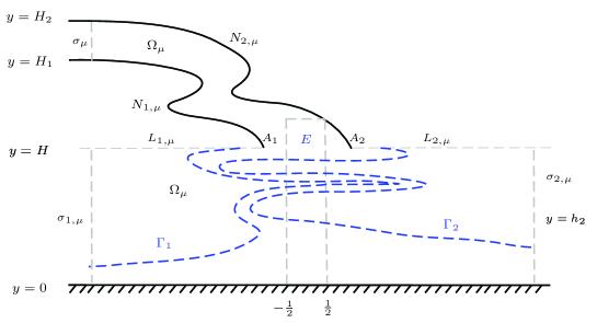
Figure 10. The domain $\displaystyle E$

∎

Set

$$\bar{\lambda}_{\mu}=\sup_{\lambda\in\Sigma_{\mu}}\lambda.$$ (2.49)

It follows from Lemma 2.11 that there exists a $\displaystyle C_{0}>0$ independent of $\displaystyle\mu$ and $\displaystyle Q_{1}$, such that

$$\frac{\max\{Q_{1}^{2},(Q-Q_{1})^{2}\}}{2H^{2}}+gH\leq\bar{\lambda}_{\mu}\leq C_{0}.$$ (2.50)

Next, we can establish the almost continuous fit conditions to the impinging jet flow under gravity.

Proposition 2.12.

(almost continuous fit conditions) For any $\displaystyle\mu>1$, there exist a $\displaystyle\bar{Q}_{1,\mu}\in\left[0,Q\right]$ and a $\displaystyle\bar{\lambda}_{\mu}\geq\frac{\max\{{\bar{Q}_{1,\mu}}^{2},(Q-\bar{Q}_{1,\mu})^{2}\}}{2H^{2}}+gH$ , such that

(1) $\displaystyle k_{1,\bar{\lambda}_{\mu},\bar{Q}_{1,\mu},\mu}(H)\leq-1$ and $\displaystyle k_{2,\bar{\lambda}_{\mu},\bar{Q}_{1,\mu},\mu}(H)\geq 1$.

(2) $\displaystyle k_{1,\bar{\lambda}_{\mu},\bar{Q}_{1,\mu},\mu}(H)=-1$ or $\displaystyle k_{2,\bar{\lambda}_{\mu},\bar{Q}_{1,\mu},\mu}(H)=1$.

(3) $\displaystyle k_{2,\bar{\lambda}_{\mu},\bar{Q}_{1,\mu},\mu}(H)=1$ for $\displaystyle\bar{Q}_{1,\mu}<Q$.

(4) $\displaystyle k_{1,\bar{\lambda}_{\mu},\bar{Q}_{1,\mu},\mu}(H)=-1$ for $\displaystyle\bar{Q}_{1,\mu}>0$.

Remark 2.4.

Obviously, as long as the critical cases $\displaystyle\bar{Q}_{1,\mu}=0$ and $\displaystyle\bar{Q}_{1,\mu}=Q$ are excluded, then the continuous fit conditions

$$k_{1,\bar{\lambda}_{\mu},\bar{Q}_{1,\mu},\mu}(H)=-1 k_{2,\bar{\lambda}_{\mu},\bar{Q}_{1,\mu},\mu}(H)=1$$ and

are satisfied. This will be done in the next section.

Proof.

(1). By using the similar arguments in Lemma 2.8, taking a sequence $\displaystyle\{\lambda_{n}\}$ with $\displaystyle\lambda_{n}\in\Sigma_{\mu}$ and $\displaystyle\lambda_{n}\uparrow\bar{\lambda}_{\mu}$, we can obtain from the definition of $\displaystyle\Sigma_{\mu}$ that there exists a sequence $\displaystyle\{Q_{1,n}\}$ with $\displaystyle Q_{1,n}\in(0,Q)$, such that

$$\text{$\displaystyle k_{1,\lambda_{n},Q_{1,n},\mu}(H)<-1\ $ and $\displaystyle\ k_{2,\lambda_{n},Q_{1,n},\mu}(H)>1$}.$$ (2.51)

It follows from the similar arguments in the proof of Lemma 2.8 that there exist two subsequences $\displaystyle\{\lambda_{n}\}$ and $\displaystyle\{Q_{1,n}\}$, such that

$$\lambda_{n}\rightarrow\bar{\lambda}_{\mu},\ Q_{1,n}\rightarrow\bar{Q}_{1,\mu},$$

and

$$\psi_{\lambda_{n},Q_{1,n},\mu}\rightharpoonup\psi_{\bar{\lambda}_{\mu},\bar{Q}_{1,\mu},\mu}\ \ \text{in $\displaystyle H^{1}(\Omega_{\mu})$ and uniformly in any compact subset of $\displaystyle\Omega_{\mu}$},$$

as $\displaystyle n\rightarrow+\infty$. Furthermore,

$$\lim_{n\rightarrow+\infty}k_{1,\lambda_{n},Q_{1,n},\mu}(H)=k_{1,\bar{\lambda}_{\mu},\bar{Q}_{1,\mu},\mu}(H)\ \text{and}\ \lim_{n\rightarrow+\infty}k_{2,\lambda_{n},Q_{1,n},\mu}(H)=k_{2,\bar{\lambda}_{\mu},\bar{Q}_{1,\mu},\mu}(H).$$

Therefore, the assertion (1) follows from (2.51).

(2). Suppose that the assertion (2) is not true. Then it follows from the assertion (1) that

$$k_{1,\bar{\lambda}_{\mu},\bar{Q}_{1,\mu},\mu}(H)<-1\ \ \text{and}\ \ k_{1,\bar{\lambda}_{\mu},\bar{Q}_{1,\mu},\mu}(H)>1.$$ (2.52)

Due to the continuous dependence of $\displaystyle k_{i,\lambda,Q_{1},\mu}(H)$ on $\displaystyle\lambda$ and $\displaystyle Q_{1}$ in Lemma 2.8, there exist $\displaystyle\lambda^{\prime}>\bar{\lambda}_{\mu}$ and $\displaystyle Q_{1}^{\prime}\in\left(0,Q\right)$ with $\displaystyle\lambda^{\prime}-\bar{\lambda}_{\mu}$ and $\displaystyle|\bar{Q}_{1,\mu}-Q_{1}^{\prime}|$ small enough, such that

$$k_{1,\lambda^{\prime},Q_{1}^{\prime},\mu}(H)<-1\ \ \text{and}\ \ k_{2,\lambda^{\prime},Q_{1}^{\prime},\mu}(H)>1.$$

Then we have that $\displaystyle\lambda^{\prime}\in\Sigma_{\mu}$, which contradicts to the definition of $\displaystyle\bar{\lambda}_{\mu}$ in (2.49).

(3). Suppose that the opposite is true. Then $\displaystyle k_{2,\bar{\lambda}_{\mu},\bar{Q}_{1,\mu},\mu}(H)>1$ for $\displaystyle\bar{Q}_{1,\mu}<Q$, and the assertion (2) implies that $\displaystyle k_{1,\bar{\lambda}_{\mu},\bar{Q}_{1,\mu},\mu}(H)=-1$. Due to Lemma 2.9, it holds that

$$\psi_{\bar{\lambda}_{\mu},Q_{1},\mu}(x,y)\geq\psi_{\bar{\lambda}_{\mu},\bar{Q}_{1,\mu},\mu}(x,y)\ \ \text{in}\ \ \Omega_{\mu},$$

for any $\displaystyle Q_{1}\in(\bar{Q}_{1,\mu},Q)$. Denote

$$\psi=\psi_{\bar{\lambda}_{\mu},\bar{Q}_{1,\mu},\mu} \psi_{1}=\psi_{\bar{\lambda}_{\mu},Q_{1},\mu}(x,y) k_{i,\bar{Q}_{1,\mu}}(y)=k_{i,\bar{\lambda}_{\mu},\bar{Q}_{1,\mu},\mu}(y) k_{i,Q_{1}}(y)=k_{i,\bar{\lambda}_{\mu},Q_{1},\mu}(y)$$, , and

for $\displaystyle i=1,2$ in the following. Therefore, $\displaystyle k_{1,Q_{1}}(H)\leq k_{1,\bar{Q}_{1,\mu}}(H)=-1$. Next, we claim that

$$k_{1,Q_{1}}(H)<k_{1,\bar{Q}_{1,\mu}}(H)=-1,$$ (2.53)

for any $\displaystyle Q_{1}\in(\bar{Q}_{1,\mu},Q)$. Suppose that there exists a $\displaystyle Q_{1}\in(\bar{Q}_{1,\mu},Q)$ such that $\displaystyle k_{1,Q_{1}}(H)=k_{1,\bar{Q}_{1,\mu}}(H)$. It follows from the results in Section 9 in [4] and Section 11 in Chapter 3 in [13] that the continuous fit condition implies the smooth fit condition. Hence, $\displaystyle N_{1,\mu}\cup\Gamma_{1,\bar{\lambda}_{\mu},\bar{Q}_{1,\mu},\mu}$ and $\displaystyle N_{1,\mu}\cup\Gamma_{1,\bar{\lambda}_{\mu},Q_{1},\mu}$ are $\displaystyle C^{1}$ at $\displaystyle A_{1}$. Furthermore, $\displaystyle\nabla\psi$ is uniformly continuous in a $\displaystyle\{\psi>0\}$-neighborhood of $\displaystyle A_{1}$, and $\displaystyle\nabla\psi_{1}$ is uniformly continuous in a $\displaystyle\{\psi_{1}>0\}$-neighborhood of $\displaystyle A_{1}$, namely,

$$-\sqrt{2\lambda-2gH}=\frac{\partial\psi}{\partial\nu}=\frac{\partial\psi_{1}}{\partial\nu}=-\sqrt{2\lambda-2gH}\ \ \ \text{at $\displaystyle A_{1}$,}$$

where $\displaystyle\nu$ is the outer normal vector. It should be noted that it’s difficult to verify the inner ball property at the point $\displaystyle A_{1}$, then one can not apply the Hopf’s lemma at $\displaystyle A_{1}$.

First, we show that

$$\Gamma_{1,\bar{\lambda}_{\mu},\bar{Q}_{1,\mu},\mu}\cap\Gamma_{1,\bar{\lambda}_{\mu},Q_{1},\mu}=\varnothing.$$ (2.54)

Suppose not, there exists a $\displaystyle X_{0}=(x_{0},y_{0})\in\Gamma_{1,\bar{\lambda}_{\mu},\bar{Q}_{1,\mu},\mu}\cap\Gamma_{1,\bar{\lambda}_{\mu},Q_{1},\mu}$. Since $\displaystyle\Gamma_{1,\bar{\lambda}_{\mu},\bar{Q}_{1,\mu},\mu}$ and $\displaystyle\Gamma_{1,\bar{\lambda}_{\mu},Q_{1},\mu}$ are analytic at $\displaystyle X_{0}$, Hopf’s lemma gives that

$$-\sqrt{2\lambda-2gy_{0}}=\frac{\partial\psi_{1}}{\partial\nu}<\frac{\partial\psi}{\partial\nu}=-\sqrt{2\lambda-2gy_{0}}\ \ \text{at}\ \ X_{0},$$

where $\displaystyle\nu$ is the outer normal vector, which leads to a contradiction.

The continuity of $\displaystyle\psi$ and $\displaystyle\psi_{1}$ implies that

$$\psi<Q\ \ \text{and}\ \ \psi_{1}<Q\ \ \text{in $\displaystyle B_{r}(A_{1})$},$$

for any small $\displaystyle r>0$.

Let $\displaystyle\mathcal{M}=B_{r}(A_{1})\cap N_{1,\mu}$. It follows from the strong maximum principle that

$$\psi<\psi_{1}\ \text{in $\displaystyle\overline{B_{r}(A_{1})}\cap\{\psi>0\}$}.$$ (2.55)

Since $\displaystyle N_{1,\mu}$ are $\displaystyle C^{2,\alpha}$ and $\displaystyle\psi=\psi_{1}=0$ on $\displaystyle\mathcal{M}$, thanks to Hopf’s lemma, one has

$$\frac{\partial\psi_{1}}{\partial\nu}<\frac{\partial\psi}{\partial\nu}\ \ \text{on}\ \ \mathcal{M},$$

where $\displaystyle\nu$ is the outer normal vector of $\displaystyle\mathcal{M}$. It follows from (2.55) that there exists a small $\displaystyle\eta_{1}>0$, such that

$$\psi_{1}\geq(1+\eta_{1})\psi\ \ \text{on $\displaystyle\partial B_{r}(A_{1})\cap\{\psi>0\}$}$$

This, together with (2.54) and (2.55), implies that there exists a small $\displaystyle\eta\in(0,\eta_{1})$ such that

$$\psi_{1}\geq(1+\eta)\psi\ \ \text{on $\displaystyle\partial(B_{r}(A_{1})\cap\{\psi>0\})$}.$$

It follows from the maximum principle that

$$\psi_{1}>(1+\eta)\psi\ \ \text{in $\displaystyle B_{r}(A_{1})\cap\{\psi>0\}$,}$$

which together with $\displaystyle\psi_{1}=\psi=0$ at $\displaystyle A_{1}$ gives that

$$-\sqrt{2\lambda-2gH}=\frac{\partial\psi_{1}}{\partial\nu}\leq(1+\eta)\frac{\partial\psi}{\partial\nu}=-(1+\eta)\sqrt{2\lambda-2gH}\ \ \ \text{at $\displaystyle A_{1}$,}$$

which leads to a contradiction. Thus, the claim (2.53) holds true.

Since $\displaystyle k_{2,\bar{Q}_{1,\mu}}(H)>1$, by using the continuous dependence of $\displaystyle k_{2,\bar{\lambda}_{\mu},Q_{1},\mu}(H)$ with respect to $\displaystyle Q_{1}$, we have

$$k_{2,Q_{1}}(H)>1\ \ \text{for small $\displaystyle Q_{1}-\bar{Q}_{1,\mu}>0$}.$$ (2.56)

In view of (2.53) and (2.56), we can obtain a contradiction to the definition of $\displaystyle\bar{\lambda}_{\mu}$ by using the continuous dependence of $\displaystyle k_{i,Q_{1}}(H)$ with respect to $\displaystyle\lambda$ and $\displaystyle Q_{1}$.

(4). Similar to (3), one can show that

$$\text{ if $\displaystyle\bar{Q}_{1,\mu}>0$, then $\displaystyle k_{1,\bar{\lambda}_{\mu},\bar{Q}_{1,\mu},\mu}(H)=-1$}.$$

∎

3. The existence of the impinging flow problem

In this section, we will give the existence of the impinging flow problem based on the previous results.

Proposition 3.1.

For any $\displaystyle Q>2\sqrt{gH^{3}}$, there exist a pair $\displaystyle(\lambda,Q_{1})$ and a solution $\displaystyle\psi_{\lambda,Q_{1}}$ to the free boundary problem (2.4) with $\displaystyle Q_{1}\in[0,Q]$ and $\displaystyle\lambda\geq\frac{\max\{Q_{1}^{2},(Q-Q_{1})^{2}\}}{2H^{2}}+gH$. Moreover,

(1) $\displaystyle\psi_{\lambda,Q_{1}}(x,y)$ is increasing with respect to $\displaystyle x$ and the free boundary $\displaystyle\Gamma_{i,\lambda,Q_{1}}$ is analytic. Furthermore, the free boundary $\displaystyle\Gamma_{i,\lambda,Q_{1}}$ can be described by a continuous function $\displaystyle x=k_{i,\lambda,Q_{1}}(y)$ for $\displaystyle y\in(h_{i},H)$, respectively, $\displaystyle i=1,2$.

(2) (almost continuous fit conditions) $\displaystyle k_{1,\lambda,Q_{1}}(H)\leq-1$ and $\displaystyle k_{2,\lambda,Q_{1}}(H)\geq 1$. Furthermore,

$$k_{1,\lambda,Q_{1}}(H)=-1\quad{\text{o}r}\quad k_{2,\lambda,Q_{1}}(H)=1,$$

and

$$k_{1,\lambda,Q_{1}}(H)=-1 Q_{1}>0 k_{2,\lambda,Q_{1}}(H)=1 Q_{1}<Q$$ if , and if .

Proof.

Let $\displaystyle\{\mu_{n}\}$ be a sequence such that $\displaystyle\mu_{n}\rightarrow+\infty$. It follows from the similar arguments in the proof of Lemma 2.8 that

$$\bar{\lambda}_{\mu_{n}}\rightarrow\lambda\ \ \text{and}\ \ \bar{Q}_{1,\mu_{n}}\rightarrow Q_{1},$$

and

$$\psi_{\bar{\lambda}_{\mu_{n}},\bar{Q}_{1,\mu_{n}},\mu_{n}}\rightarrow\psi_{\lambda,Q_{1}}\ \text{weakly in $\displaystyle H_{loc}^{1}(\Omega)$ and uniformly in any compact subset of $\displaystyle\Omega$}.$$

It follows from (2.50) that

$$\lambda\leq C_{0}.$$ (3.1)

Next, we will show that $\displaystyle\psi_{\lambda,Q_{1}}$ is a local minimizer to the variational problem $\displaystyle(P_{\lambda,Q_{1}})$ (see Remark 6.1). Set $\displaystyle\psi_{n}=\psi_{\bar{\lambda}_{\mu_{n}},\bar{Q}_{1,\mu_{n}},\mu_{n}}$. We first claim that

$$\begin{array}[]{rl}&\int_{E}|\nabla\psi_{n}|^{2}+(2\bar{\lambda}_{\mu_{n}}-2gy)\chi_{\{0<\psi_{n}<Q\}\cap D}dxdy\\ \leq&\int_{E}|\nabla\tilde{\psi}|^{2}+(2\bar{\lambda}_{\mu_{n}}-2gy)\chi_{\{0<\tilde{\psi}<Q\}\cap D}dxdy,\end{array}$$ (3.2)

for any $\displaystyle\tilde{\psi}\in H^{1}(E)$ and $\displaystyle\tilde{\psi}=\psi_{n}$ on $\displaystyle\partial E$, provided that $\displaystyle n$ is sufficiently large, where $\displaystyle E$ is any compact subset of $\displaystyle\Omega$. In fact, there exists a $\displaystyle N>0$, such that $\displaystyle E\subset\Omega_{\mu_{n}}$ for any $\displaystyle n>N$. Extend $\displaystyle\tilde{\psi}=\psi_{n}$ outside of $\displaystyle E$ such that $\displaystyle\tilde{\psi}=\Psi_{\bar{\lambda}_{\mu_{n}},\mu_{n}}(y)$ on $\displaystyle\partial\Omega_{\mu_{n}}$, then it implies that (3.2) is valid.

With the aid of (3.2), by using the similar arguments in Step 4 in the proof of Lemma 2.8, one can conclude that $\displaystyle\psi_{\lambda,Q_{1}}$ is a local minimizer to the variational problem $\displaystyle(P_{\lambda,Q_{1}})$, and thus it follows from Proposition 2.2 that $\displaystyle\psi_{\lambda,Q_{1}}$ is harmonic in $\displaystyle\Omega\cap\{0<\psi_{\lambda,Q_{1}}<Q\}$ and the free boundary $\displaystyle\Gamma_{i,\lambda,Q_{1}}$ is analytic with $\displaystyle|\nabla\psi_{\lambda,Q_{1}}|=\sqrt{2\lambda-2gy}$ on $\displaystyle\Gamma_{i,\lambda,Q_{1}}$. Furthermore, Lemma 2.5 gives that the local minimizer $\displaystyle\psi_{\lambda,Q_{1}}(x,y)$ is increasing with respect to $\displaystyle x$. By using similar arguments as in Lemma 2.7, one can conclude that the free boundary $\displaystyle\Gamma_{i,\lambda,Q_{1}}$ of $\displaystyle\psi_{\lambda,Q_{1}}$ can be described by a generalized continuous function $\displaystyle x=k_{i,\lambda,Q_{1}}(y)$ ($\displaystyle i=1,2$), namely, $\displaystyle k_{i,\lambda,Q_{1}}(y+0)=\lim_{t\rightarrow y+0}k_{i,\lambda,Q_{1}}(t)$ and $\displaystyle k_{i,\lambda,Q_{1}}(y-0)=\lim_{t\rightarrow y-0}k_{i,\lambda,Q_{1}}(t)$ exist and may be infinite, and $\displaystyle k_{i,\lambda,Q_{1}}(y+0)=k_{i,\lambda,Q_{1}}(y-0)\in[-\infty,+\infty]$ for and $\displaystyle y\in(h_{i},H)$.

Next, we will show that

$$\text{ $\displaystyle k_{1,\lambda,Q_{1}}(H)=-1$ for $\displaystyle Q_{1}>0$, and $\displaystyle k_{2,\lambda,Q_{1}}(H)=1$ for $\displaystyle Q_{1}<Q$}.$$ (3.3)

If not, without loss of generality, one may assume that $\displaystyle k_{1,\lambda,Q_{1}}(H)\neq-1$ for $\displaystyle Q_{1}>0$. Since $\displaystyle Q_{1}>0$, so $\displaystyle\bar{Q}_{1,\mu_{n}}>0$ for sufficiently large $\displaystyle n$, and it follows from Lemma 2.12 that $\displaystyle k_{1,\bar{\lambda}_{\mu_{n}},\bar{Q}_{1,\mu_{n}},\mu_{n}}(H)=-1$. Similar to the Step 5 in the proof of Lemma 2.8, one can obtain a contradiction by using the convergence of the free boundary and the Cauchy-Kovalevskaya theorem.

∎

Next, $\displaystyle k_{i,\lambda,Q_{1}}(y)$ has the following properties for $\displaystyle i=1,2$.

Proposition 3.2.

The free boundary $\displaystyle\Gamma_{i,\lambda,Q_{1}}:x=k_{i,\lambda,Q_{1}}(y)$ is a bounded continuous function for any $\displaystyle x\in(h_{i},H]$, where $\displaystyle h_{i}$ is determined uniquely by (2.5) for $\displaystyle i=1,2$. Furthermore,

$$\lim_{y\rightarrow h_{1}^{+}}k_{1,\lambda,Q_{1}}(y)=-\infty Q_{1}>0 \lim_{y\rightarrow h_{2}^{+}}k_{2,\lambda,Q_{1}}(y)=+\infty Q_{1}<Q$$ if , and if .

Proof.

Consider first that $\displaystyle Q_{1}<Q$. In this case, $\displaystyle h_{2}\in(0,H)$. It follows from (2) in Proposition 3.1 that $\displaystyle k_{2,\lambda,Q_{1}}(H)=1$, and thus $\displaystyle k_{2,\lambda,Q_{1}}(y)$ is finite near $\displaystyle y=H$. It remains to show that

$$\text{$\displaystyle k_{2,\lambda,Q_{1}}(y)$ is continuous and finite in $\displaystyle(h_{2},H)$ and $\displaystyle\lim_{y\rightarrow h_{2}^{+}}k_{2,\lambda,Q_{1}}(y)=+\infty$},$$ (3.4)

which will be proved in three steps.

Step 1. Let $\displaystyle(\beta_{i},\alpha_{i})$ be the maximal intervals ($\displaystyle i=1,2,\cdot\cdot\cdot$), such that $\displaystyle k_{2,\lambda,Q_{1}}(y)$ is finite valued, $\displaystyle\alpha_{1}=H$ and $\displaystyle\beta_{i}\geq\alpha_{i+1}$. We first claim that

the number of intervals $$(\beta_{i},\alpha_{i})$$ is finite.

If not, then $\displaystyle\alpha_{i}-\beta_{i}\rightarrow 0$ and $\displaystyle\beta_{i}-\alpha_{i+1}\rightarrow 0$ as $\displaystyle i\rightarrow+\infty$. There are the following two cases to be considered.

Case 1. $\displaystyle k_{2,\lambda,Q_{1}}(\alpha_{i}-0)=k_{2,\lambda,Q_{1}}(\beta_{i}+0)=-\infty$. (See Figure 11)

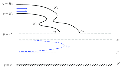
Figure 11. Case 1

Denote $\displaystyle G_{i}\subset\{(x,y)\in D\mid x<k_{2,\lambda,Q_{1}}(y),\beta_{i}<y<\alpha_{i}\}$, such that $\displaystyle G_{i}$ satisfies

$$\forall\ X_{1}=(x_{1},y_{1})\in G_{i},\ \ \exists\ y_{0}\ \ \text{such that}\ \ x_{1}=k_{2,\lambda,Q_{1}}(y_{0})\ \ \text{and}\ \ X_{0}=(x_{1},y_{0})\in\Gamma_{2,\lambda,Q_{1}}.$$

Thanks to the Lipschitz continuity of $\displaystyle\psi_{\lambda,Q_{1}}$, we have

$$Q-\psi_{\lambda,Q_{1}}(X_{1})=\psi_{\lambda,Q_{1}}(X_{0})-\psi_{\lambda,Q_{1}}(X_{1})\leq C(\alpha_{i}-\beta_{i}),$$

which implies that

$$\psi_{\lambda,Q_{1}}(X_{1})>0 X_{1}\in G_{i}$$ for any , (3.5)

provided that $\displaystyle\beta_{i}-\alpha_{i}$ is small enough such that $\displaystyle C(\alpha_{i}-\beta_{i})<Q$.

Hence, we can derive a contradiction to the non-oscillation Lemma 2.6 in the region $\displaystyle G_{i}\cap\{-2R<x<-R\}$ (for some $\displaystyle R$ sufficiently large) provided that $\displaystyle\alpha_{i}-\beta_{i}$ is small enough.

Case 2. $\displaystyle k_{2,\lambda,Q_{1}}(\alpha_{i}-0)=+\infty$ or $\displaystyle k_{2,\lambda,Q_{1}}(\beta_{i}+0)=+\infty$. Without loss of generality, we assume that $\displaystyle k_{2,\lambda,Q_{1}}(\beta_{i}+0)=+\infty$ and consider the following two subcases.

Subcase 2.1. $\displaystyle k_{2,\lambda,Q_{1}}(\alpha_{i+1}-0)=+\infty$ (see Figure 12).

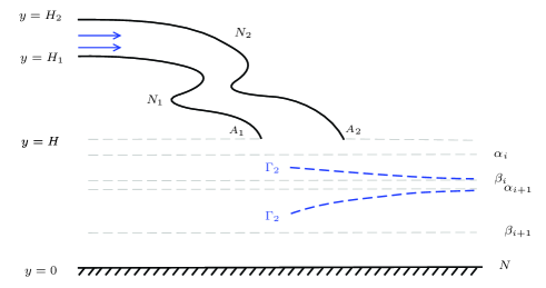
Figure 12. Subcase 2.1

For sufficiently large $\displaystyle R>0$, set

$$G_{i,R}=\left\{(x,y)\in D\mid x>R,\frac{\alpha_{i+1}+\beta_{i+1}}{2}<y<\frac{\alpha_{i}+\beta_{i}}{2}\right\}.$$

Similar to (3.5), we can conclude that $\displaystyle\psi_{\lambda,Q_{1}}>0$ in $\displaystyle G_{i,R}$ for sufficiently large $\displaystyle i$. This leads to a contradiction by using the non-oscillation Lemma 2.6 in the region $\displaystyle G_{i,R}\cap\{x<2R\}$.

Subcase 2.2. $\displaystyle k_{2,\lambda,Q_{1}}(\alpha_{i+1}-0)=-\infty$ (see Figure 13).

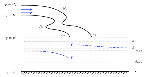
Figure 13. Subcase 2.2

By using the monotonicity of $\displaystyle\psi_{\lambda,Q_{1}}(x,y)$ with respect to $\displaystyle x$, we have that $\displaystyle\psi_{\lambda,Q_{1}}=Q$ on $\displaystyle\{y=\alpha_{i+1}\}$, and thus the line $\displaystyle\{y=\alpha_{i+1}\}$ is the free boundary of $\displaystyle\psi_{\lambda,Q_{1}}$. It follows from Proposition 2.2 that

$$\psi_{\lambda,Q_{1}}=Q\ \text{and}\ \frac{\partial\psi_{\lambda,Q_{1}}}{\partial y}=\sqrt{2\lambda-2g\alpha_{i+1}}\ \text{on}\ \ \{y=\alpha_{i+1}\},$$

which contradicts to the Cauchy-Kovalevskaya theorem.

Hence, we can conclude that the number of $\displaystyle(\alpha_{i},\beta_{i})$ is finite.

Step 2. In this step, we will show that

$$\text{the number of $\displaystyle(\alpha_{i},\beta_{i})$ is in fact one, namely, $\displaystyle i=1$}.$$ (3.6)

If not, the number of the intervals $\displaystyle(\beta_{i},\alpha_{i})$ is at least 2. Then there are the following three cases.

Case 1. $\displaystyle k_{2,\lambda,Q_{1}}(\beta_{1}+0)=k_{2,\lambda,Q_{1}}(\alpha_{2}-0)=+\infty$.

The non-oscillation Lemma 2.6 gives that $\displaystyle\alpha_{2}<\beta_{1}$. We first claim that

$$k_{1,\lambda,Q_{1}}(y)<+\infty \alpha_{2}<y<\beta_{1}$$ for any . (3.7)

If not, without loss of generality, one may assume that there exists a $\displaystyle\beta_{0}\in(\alpha_{2},\beta_{1})$, such that

$$\lim_{y\rightarrow\beta_{0}^{+}}k_{1,\lambda,Q_{1}}(y)=+\infty\ \ \text{and}\ \ k_{1,\lambda,Q_{1}}(y)<+\infty\ \ \text{for}\ \ y\in(\beta_{0},\beta_{1}).$$

Since $\displaystyle k_{2,\lambda,Q_{1}}(\beta_{1}+0)=k_{1,\lambda,Q_{1}}(\beta_{0}+0)=+\infty$, we conclude that the free boundaries $\displaystyle\Gamma_{1,\lambda,Q_{1}}$ and $\displaystyle\Gamma_{2,\lambda,Q_{1}}$ satisfy the flatness condition (see Section 7 in [1]) near $\displaystyle y=\beta_{0}$ and $\displaystyle y=\beta_{1}$. Then there exists a large $\displaystyle x_{0}>0$, such that

$$\Gamma_{1,\lambda,Q_{1}}\cap\{(x,y)\mid x>x_{0},\beta_{0}<y<\beta_{1}\} y=g_{1}(x) g_{1}(x)\downarrow\beta_{0}$$ is described by , and

as $\displaystyle x\rightarrow+\infty$, and

$$\Gamma_{2,\lambda,Q_{1}}\cap\{(x,y)\mid x>x_{0},\beta_{1}<y<\alpha_{1}\} y=g_{2}(x) g_{2}(x)\downarrow\beta_{1}$$ is described by , and

as $\displaystyle x\rightarrow+\infty$. Furthermore, it holds that

$$g^{\prime}_{i}(x)\rightarrow 0\ \text{ as}\ \ x\rightarrow+\infty,\ \ \ \left|g_{i}^{(j)}(x)\right|\leq C\ \ \text{for}\ \ i=1,2,j=2,3.$$

Due to the uniform elliptic estimates, there exists a sequence $\displaystyle\{\psi_{\lambda,Q_{1}}(x+n,y)\}$, such that

$$\psi_{\lambda,Q_{1}}(x+n,y)\rightarrow\psi_{0}(x,y),\quad\text{in}\ C^{2,\alpha}(\mathbb{T})$$

where $\displaystyle\mathbb{T}=\{-\infty<x<+\infty\}\times\{\beta_{0}<y<\beta_{1}\}$, and

$$\left\{\begin{array}[]{ll}&\Delta\psi_{0}=0\quad\quad\text{in}~{}~{}\mathbb{T},\\ &\frac{\partial\psi_{0}(x,\beta_{0})}{\partial y}=\sqrt{2\lambda-2g\beta_{0}}\ \ \text{and}\ \ \frac{\partial\psi_{0}(x,\beta_{1})}{\partial y}=\sqrt{2\lambda-2g\beta_{1}},\\ &\psi_{0}(x,\beta_{0})=0\ \text{and}\ \psi_{0}(x,\beta_{1})=Q.\end{array}\right.$$ (3.8)

A direct computation gives that

$$\psi_{0}(y)=\sqrt{2\lambda-2g\beta_{1}}(y-\beta_{1})+Q\quad\quad\text{for}\ \beta_{0}<y<\beta_{1},$$

and

$$\frac{\partial\psi_{0}(x,\beta_{1})}{\partial y}=\sqrt{2\lambda-2g\beta_{1}}\quad\quad\text{for}\ -\infty<x<+\infty,$$

which contradicts to $\displaystyle\frac{\partial\psi_{0}(x,\beta_{1})}{\partial y}=\sqrt{2\lambda-2g\beta_{0}}$, due to $\displaystyle\sqrt{2\lambda-2g\beta_{1}}<\sqrt{2\lambda-2g\beta_{0}}$.

Denote

$$G_{R}=\{(x,y)\in D\mid R<x<2R,\alpha_{2}<y<H\}$$

for sufficiently large $\displaystyle R>0$. Then it follows from the claim (3.7) that $\displaystyle\psi_{\lambda,Q_{1}}>0$ in $\displaystyle G_{R}$, which contradicts to the non-oscillation Lemma 2.6 in $\displaystyle G_{R}$.

Case 2. $\displaystyle k_{2,\lambda,Q_{1}}(\beta_{1}+0)=-k_{2,\lambda,Q_{1}}(\alpha_{2}-0)=+\infty$.

Due to the monotonicity of $\displaystyle\psi_{\lambda,Q_{1}}$ with respect to $\displaystyle x$, it follows from Proposition 2.2 that

$$\psi_{\lambda,Q_{1}}=Q\ \text{and}\ \frac{\partial\psi_{\lambda,Q_{1}}}{\partial y}=-\sqrt{2\lambda-2g\alpha_{2}}\quad\text{on}\ \{y=\alpha_{2}\},$$

which contradicts to the Cauchy-Kovalevskaya theorem.

Case 3. $\displaystyle k_{2,\lambda,Q_{1}}(\beta_{1}+0)=-k_{2,\lambda,Q_{1}}(\alpha_{2}-0)=-\infty$.

Similarly to Case 2, one can get

$$\psi_{\lambda,Q_{1}}=Q\ \text{and}\ \frac{\partial\psi_{\lambda,Q_{1}}}{\partial y}=\sqrt{2\lambda-2g\beta_{1}}\quad\text{on}\ \{y=\beta_{1}\},$$

which also leads to a contradiction.

Case 4. $\displaystyle k_{2,\lambda,Q_{1}}(\beta_{1}+0)=k_{2,\lambda,Q_{1}}(\alpha_{2}-0)=-\infty$.

There are the following two subcases.

Subcase 4.1. $\displaystyle k_{2,\lambda,Q_{1}}(\beta_{2}+0)=-\infty$. We first claim that

$$k_{1,\lambda,Q_{1}}(y)=-\infty\ \ \text{for any}\ \ \beta_{2}<y<\alpha_{2}.$$ (3.9)

If not, without loss of generality, we assume that there exists a $\displaystyle\beta_{0}\in(\beta_{2},\alpha_{2})$, such that

$$\lim_{y\rightarrow\beta_{0}^{+}}k_{1,\lambda,Q_{1}}(y)=-\infty\ \ \text{and}\ \ k_{1,\lambda,Q_{1}}(y)>-\infty\ \ \text{for}\ \ y\in(\beta_{0},\beta_{0}+\varepsilon)\ \text{and small $\displaystyle\varepsilon>0$}.$$

Similar to Case 1 in Step 2, there exists a sequence $\displaystyle\{\psi_{\lambda,Q_{1}}(x-n,y)\}$, such that

$$\psi_{\lambda,Q_{1}}(x-n,y)\rightarrow\psi_{0}(x,y),\quad\quad\text{in}\ \ C^{2,\alpha}\left(\{x<k_{2,\lambda,Q_{1}}(y),\beta_{2}<y<\alpha_{2}\}\right),$$

and $\displaystyle\psi_{0}$ satisfies (3.8), which leads to a contradiction. The claim (3.9) implies that

$$\psi_{\lambda,Q_{1}}>0\ \ \text{in}\ \ \{(x,y)\in D\mid x<k_{2,\lambda,Q_{1}}(y),\beta_{2}<y<\alpha_{2}\},$$

which contradicts to the non-oscillation Lemma 2.6.

Subcase 4.2. $\displaystyle k_{2,\lambda,Q_{1}}(\beta_{2}+0)=+\infty$. Similar to the claim (3.9), one can get

$$k_{1,\lambda,Q_{1}}(y)=-\infty\ \ \text{for any}\ \ 0<y<\alpha_{2}.$$ (3.10)

The non-oscillation Lemma 2.6 yields that

$$k_{2,\lambda,Q_{1}}(y)=+\infty\ \ \text{for any}\ \ 0<y<\beta_{2}.$$ (3.11)

With the aid of (3.10) and (3.11), by using the similar arguments in Case 1 in Step 2, one can get a sequence $\displaystyle\{\psi_{\lambda,Q_{1}}(x+n,y)\}$, such that

$$\psi_{\lambda,Q_{1}}(x+n,y)\rightarrow\psi_{1}(x,y),\quad\ \ \text{in}\ ~{}~{}C^{2,\alpha}\left(\{-\infty<x<+\infty\}\times\{0<y<\beta_{2}\}\right),$$

and $\displaystyle\psi_{1}$ satisfies

$$\left\{\begin{array}[]{ll}&\Delta\psi_{1}=0\ \ \text{in}\ ~{}~{}\{-\infty<x<+\infty\}\times\{0<y<\beta_{2}\},\\ &\frac{\partial\psi_{1}(x,\beta_{2})}{\partial y}=\sqrt{2\lambda-2g\beta_{2}},\ \ \psi_{1}(x,\beta_{2})=Q.\end{array}\right.$$

By the uniqueness for the Cauchy-Kovalevskaya theorem, one has

$$\psi_{1}(x,y)=\sqrt{2\lambda-2g\beta_{2}}(y-\beta_{2})+Q\ \ \text{in}\ \{-\infty<x<+\infty\}\times\{0<y<\beta_{2}\}.$$ (3.12)

It follows from Lemma 2.4 that

$$\max\{-\sqrt{2\lambda-2gh_{1}}y+Q_{1},0\}\leq\psi_{1}(x,y)\leq\min\{\sqrt{2\lambda-2gh_{2}}y+Q_{1},Q\}$$

in $\displaystyle D$, which implies that $\displaystyle\psi_{1}(x,0)=Q_{1}$. Hence

$$Q-Q_{1}=\sqrt{2\lambda-2g\beta_{2}}\beta_{2}.$$ (3.13)

Similarly, there exists a sequence $\displaystyle\{\psi_{\lambda,Q_{1}}(x-n,y)\}$, such that

$$\psi_{\lambda,Q_{1}}(x-n,y)\rightarrow\psi_{2}(x,y),\quad\text{in}\ C^{2,\alpha}(\mathbb{T}),$$

where $\displaystyle\mathbb{T}=\{-\infty<x<+\infty\}\times\{0<y<\alpha_{2}\}$, and $\displaystyle\psi_{2}$ satisfies

$$\left\{\begin{array}[]{ll}&\Delta\psi_{2}=0\quad\quad\text{in}~{}~{}\mathbb{T},\\ &\frac{\partial\psi_{2}(x,\alpha_{2})}{\partial y}=\sqrt{2\lambda-2g\alpha_{2}},\ \ \psi_{2}(x,\alpha_{2})=Q.\end{array}\right.$$

It implies that

$$Q-Q_{1}=\sqrt{2\lambda-2g\alpha_{2}}\alpha_{2}.$$ (3.14)

It follows from (3.13) and (3.14) that we obtain a contradiction to $\displaystyle\alpha_{2}>\beta_{2}$.

Hence, we have shown that

$$\text{$\displaystyle k_{2,\lambda,Q_{1}}(y)$ is continuous and finite in $\displaystyle(\beta_{1},H)$ and infinite in $\displaystyle(0,\beta_{1})$}.$$

Furthermore,

$$\text{$\displaystyle\lim_{y\rightarrow\beta_{1}^{+}}k_{2,\lambda,Q_{1}}(y)=+\infty$}.$$ (3.15)

Step 3. In this step, we will show that

$$\beta_{1}=h_{2}.$$

Due to (3.15), it follows from the similar arguments in Case 1 in Step 1 that there exists a sequence $\displaystyle\{\psi_{\lambda,Q_{1}}(x+n,y)\}$, such that

$$\psi_{\lambda,Q_{1}}(x+n,y)\rightarrow\psi_{0}(x,y)\quad\quad\text{in}\ C^{2,\alpha}(\mathbb{T}),$$

where $\displaystyle\mathbb{T}=\{-\infty<x<+\infty\}\times\{0<y<\beta_{1}\}$, and

$$\left\{\begin{array}[]{ll}&\Delta\psi_{0}=0\quad\quad\text{in}~{}~{}\mathbb{T},\\ &\frac{\partial\psi_{0}(x,\beta_{1})}{\partial y}=\sqrt{2\lambda-2g\beta_{1}}\ \text{and}\ \psi_{0}(x,\beta_{1})=Q\ \ \text{for $\displaystyle-\infty<x<+\infty$}.\end{array}\right.$$

Similar arguments in the proof in Subcase 4.2 in Step 2 show

$$Q-Q_{1}=\sqrt{2\lambda-2g\beta_{1}}\beta_{1}.$$

This and Proposition 2.1 give $\displaystyle\beta_{1}=h_{2}$.

Next we consider the case that $\displaystyle Q_{1}=Q$. It follows from similar arguments above that

$$\text{$\displaystyle k_{1,\lambda,Q_{1}}(y)$ is continuous and finite in $\displaystyle(h_{1},H)$ and $\displaystyle\lim_{y\rightarrow h_{1}^{+}}k_{1,\lambda,Q_{1}}(y)=-\infty$}.$$

Finally, using the non-oscillation Lemma 2.6, one can show that

$$h_{2}=0,\ \ \ \text{$\displaystyle k_{2,\lambda,Q_{1}}(y)$ is continuous and finite in $\displaystyle(0,H)$}.$$

∎

The previous result gives the almost continuous fit conditions. The continuous fit conditions will follow once the critical value $\displaystyle Q_{1}=0$ or $\displaystyle Q_{1}=Q$ can be excluded.

Proposition 3.3.

The value $\displaystyle Q_{1}$ in Proposition 3.1 lies in $\displaystyle(0,Q)$.

Proof.

Without loss of generality, we assume that $\displaystyle Q_{1}=0$, which implies that $\displaystyle h_{2}\in(0,H)$. The non-oscillation Lemma 2.6 gives that

$$k_{1,\lambda,0}(0)=\lim_{y\rightarrow 0^{+}}k_{1,\lambda,0}(y)\ \text{exists}.$$

Next, we consider the following three cases.

Case 1. $\displaystyle k_{1,\lambda,0}(0)=+\infty$ (see Figure 14).

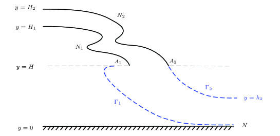
Figure 14. Case 1.

Since $\displaystyle k_{2,\lambda,0}(h_{2})=+\infty$, it follows from the similar arguments in Case 1 in Step 2 in the proof of Proposition 3.2 that there exists a sequence $\displaystyle\{\psi_{\lambda,0}(x+n,y)\}$, such that

$$\psi_{\lambda,0}(x+n,y)\rightarrow\psi_{0}(x,y)\quad\quad\text{in}\ C^{2,\alpha}(\{-\infty<x<+\infty\}\times\{0<y<h_{2}\}),$$

and $\displaystyle\psi_{0}$ satisfies

$$\left\{\begin{array}[]{ll}&\Delta\psi_{0}=0\quad\quad\text{in}~{}~{}\{-\infty<x<+\infty\}\times\{0<y<h_{2}\},\\ &\frac{\partial\psi_{0}(x,0+0)}{\partial y}=\sqrt{2\lambda}\ \ \text{and}\ \ \frac{\partial\psi_{0}(x,h_{2}-0)}{\partial y}=\sqrt{2\lambda-2gh_{2}},\\ &\psi_{0}(x,0)=0\ \text{and}\ \psi_{0}(x,h_{2})=Q.\end{array}\right.$$

This is an overdetermined problem, due to $\displaystyle\sqrt{2\lambda-2gh_{2}}<\sqrt{2\lambda}$.

Case 2. $\displaystyle k_{1,\lambda,0}(0)=-\infty$ (see Figure 15).

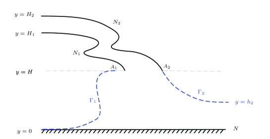
Figure 15. Case 2.

The maximum principle gives that

$$\frac{\partial\psi_{\lambda,0}}{\partial y}\geq 0\ \ \text{on}\ \ N.$$

Similar to the Case 1 in the proof of Proposition 3.2, one can obtain a contradiction by using the non-oscillation Lemma 2.6 and Remark 2.3 for $\displaystyle\psi_{\lambda,0}$ in $\displaystyle D\cap\{-2R<x<-R\}\cap\{\psi_{\lambda,0}>0\}$, provided that $\displaystyle R$ is sufficiently large.

Case 3. $\displaystyle k_{1,\lambda,0}(0)\in(-\infty,+\infty)$ (see Figure 16).

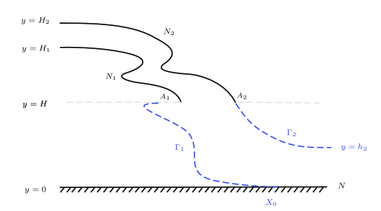
Figure 16. Case 3.

Set $\displaystyle X_{0}=(k_{1,\lambda,0}(0),0)$. It follows from the results in Section 9 in [4] and Section 11 in Chapter 3 in [13] that the continuous fit conditions imply the smooth fit conditions, we have that the free boundary $\displaystyle\Gamma_{1,\lambda,0}$ is $\displaystyle C^{1}$-smooth at $\displaystyle X_{0}$. Furthermore, $\displaystyle\nabla\psi_{\lambda,0}$ is uniformly continuous in a $\displaystyle\{\psi_{\lambda,0}>0\}$-neighborhood of $\displaystyle X_{0}$, and thus

$$|\nabla\psi_{\lambda,0}|=\frac{\partial\psi_{\lambda,0}}{\partial y}=\sqrt{2\lambda} X_{0}$$ at .

Consider a function

$$\omega_{0}(x,y)=\min\{\gamma y,Q\} \gamma=\frac{\sqrt{2\lambda-2gh_{2}}+\sqrt{2\lambda}}{2}$$ for .

It follows from the Step 3 in the proof of Proposition 3.1 that

$$\psi_{\lambda,0}(x,y)\rightarrow\min\{\sqrt{2\lambda-2gh_{2}}y,Q\}\ \ \text{as}\ \ x\rightarrow+\infty.$$

Since $\displaystyle\gamma>\sqrt{2\lambda-2gh_{2}}$, so $\displaystyle\psi_{\lambda,0}\leq\omega_{0}$ in the far field, which together with the maximum principle gives that

$$\psi_{\lambda,0}(x,y)\leq\omega_{0}(x,y)\ \ \text{in}\ \ D\cap\{\omega_{0}<Q\}.$$

In view of $\displaystyle\psi_{\lambda,0}=\omega_{0}=0$ at $\displaystyle X_{0}$, thus we have

$$\sqrt{2\lambda}=\frac{\partial\psi_{\lambda,0}}{\partial y}=\frac{\partial\psi_{\lambda,0}}{\partial\nu}\leq\frac{\partial\omega_{0}}{\partial\nu}=\frac{\partial\omega_{0}}{\partial y}=\gamma=\frac{\sqrt{2\lambda-2gh_{2}}+\sqrt{2\lambda}}{2}\ \ \text{at}\ \ X_{0},$$

which leads to a contradiction, due to $\displaystyle h_{2}>0$.

∎

Remark 3.1.

Proposition 3.3 implies that the impinging jet under gravity with continuous fit conditions must possess two asymptotic directions in far fields. This conclusion coincides the results on impinging jet in absence of gravity in [10].

As a consequence of Proposition 3.1-Proposition 3.3, we can get

Theorem 3.4.

For any $\displaystyle Q>2\sqrt{gH^{3}}$, there exist an effluent flux $\displaystyle Q_{1}\in(0,Q)$ and a $\displaystyle\lambda>\frac{\max\{Q_{1}^{2},(Q-Q_{1})^{2}\}}{2H^{2}}+gH$, such that there exists a solution $\displaystyle(u,v,p,\Gamma_{1},\Gamma_{2})$ to the impinging jet flow problem, where

$$u=\frac{\partial\psi_{\lambda,Q_{1}}}{\partial y},\ v=-\frac{\partial\psi_{\lambda,Q_{1}}}{\partial x}\ \text{and}\ p=p_{atm}+\lambda-\frac{|\nabla\psi_{\lambda,Q_{1}}|^{2}}{2}-gy,$$

and

$$\Gamma_{i}=\Gamma_{i,\lambda,Q_{1}}:x=k_{i,\lambda,Q_{1}}(y)=k_{i}(y)\ \text{for $\displaystyle y\in(h_{i},H)$ and $\displaystyle i=1,2$}.$$

Proof.

It follows from Proposition 3.1 and Proposition 3.3 that

$$\ Q_{1}\in(0,Q)\ \ \text{and}\ \ \lambda\geq\frac{\max\{Q_{1}^{2},(Q-Q_{1})^{2}\}}{2H^{2}}+gH.$$

Furthermore, Proposition 3.1 and Proposition 3.2 give that

$$k_{1,\lambda,Q_{1}}(H)=-1\ \ \text{and}\ \ k_{2,\lambda,Q_{1}}(H)=1,$$

and

$$\text{$\displaystyle\lim_{y\rightarrow h_{1}^{+}}k_{1,\lambda,Q_{1}}(y)=-\infty$ and $\displaystyle\lim_{y\rightarrow h_{2}^{+}}k_{2,\lambda,Q_{1}}(y)=+\infty$},$$

where $\displaystyle h_{1}$ and $\displaystyle h_{2}$ are uniquely determined by (2.5). It follows from Lemma 6.5 in the appendix that the free boundary $\displaystyle\Gamma_{1,\lambda,Q_{1}}$ and $\displaystyle\Gamma_{2,\lambda,Q_{1}}$ are analytic, and the Bernoulli’s law gives that $\displaystyle p=p_{atm}$ on $\displaystyle\Gamma_{1,\lambda,Q_{1}}\cup\Gamma_{2,\lambda,Q_{1}}$.

Next, we will show that $\displaystyle\lambda>\frac{\max\{Q_{1}^{2},(Q-Q_{1})^{2}\}}{2H^{2}}+gH$. If not, without loss of generality, one may assume that $\displaystyle Q_{1}\geq\frac{Q}{2}>\sqrt{gH^{3}}$ and $\displaystyle\lambda=\frac{Q_{1}^{2}}{2H^{2}}+gH$. Since $\displaystyle Q_{1}=\sqrt{2\lambda-2gh_{1}}h_{1}$, it follows from the proof of Proposition 2.1 that $\displaystyle h_{1}=H$. This implies that the free boundary $\displaystyle\Gamma_{1,\lambda,Q_{1}}$ is empty, which leads to a contradiction.

Therefore, the continuous fit conditions are fulfilled for the free boundary $\displaystyle\Gamma_{i,\lambda,Q_{1}}$ at $\displaystyle A_{i}$ ($\displaystyle i=1,2$). It follows from the results in Section 9 in [4] and Section 11 in Chapter 3 in [13] that the continuous fit conditions imply the smooth fit conditions, hence, $\displaystyle N_{i}\cup\Gamma_{i,\lambda,Q_{1}}$ is $\displaystyle C^{1}$-smooth at $\displaystyle A_{i}$, that is

$$k_{1,\lambda,Q_{1}}^{\prime}(H-0)=g^{\prime}_{1}(H+0)\ \ \text{and}\ \ k_{2,\lambda,Q_{2}}(H-0)=g^{\prime}_{2}(H+0).$$

Furthermore, $\displaystyle\nabla\psi_{\lambda,Q}$ is uniformly continuous in a $\displaystyle\{\psi_{\lambda,Q_{1}}>0\}$-neighborhood of $\displaystyle A_{1}$, and $\displaystyle\nabla\psi_{\lambda,Q_{1}}$ is uniformly continuous in a $\displaystyle\{\psi_{\lambda,Q_{1}}<Q\}$-neighborhood of $\displaystyle A_{2}$.

It remains to show that

$$v=-\frac{\partial\psi_{\lambda,Q_{1}}}{\partial x}<0\ \quad\text{in}~{}~{}(\Omega\cap\{0<\psi_{\lambda,Q_{1}}<Q\})\cup\Gamma_{1,\lambda,Q_{1}}\cup\Gamma_{2,\lambda,Q_{1}}.$$ (3.16)

By virtue of the monotonicity of $\displaystyle\psi_{\lambda,Q_{1}}$ with respect to $\displaystyle x$, one has

$$\psi_{\lambda,Q_{1}}(x_{1},y)\geq\psi_{\lambda,Q_{1}}(x_{2},y)\ \ \text{for any}\ \ x_{1}\geq x_{2},$$

which implies that

$$-\frac{\partial\psi_{\lambda,Q_{1}}}{\partial x}\leq 0 \Omega_{0}=\Omega\cap\{0<\psi_{\lambda,Q_{1}}<Q\}$$ in .

Consider $\displaystyle v=-\frac{\partial\psi_{\lambda,Q_{1}}}{\partial x}$ in $\displaystyle\Omega_{0}$, which solves the Laplace equation in $\displaystyle\Omega_{0}$. The strong maximum principle gives that $\displaystyle v<0$ in $\displaystyle\Omega_{0}$. Finally, we claim that

$$v<0\ \ \ \text{on}~{}~{}\Gamma_{1,\lambda,Q_{1}}\cup\Gamma_{2,\lambda,Q_{1}}.$$

If not, without loss of generality, suppose that there exists a $\displaystyle X_{0}=(x_{0},y_{0})\in\Gamma_{2,\lambda,Q_{1}}$, such that $\displaystyle v(X_{0})=0$. Since the free boundary $\displaystyle\Gamma_{2,\lambda,Q_{1}}$ is analytic at $\displaystyle X_{0}$, we can assume that $\displaystyle\nu=(0,1)$ is the outer normal vector to $\displaystyle\Gamma_{2,\lambda,Q_{1}}$ at $\displaystyle X_{0}$. Then Hopf’s lemma implies that

$$v_{y}=\frac{\partial v}{\partial\nu}>0\ \ \text{at}\ \ X_{0}.$$ (3.17)

It follows from Proposition 2.2 that $\displaystyle u^{2}+v^{2}=|\nabla\psi_{\lambda,Q_{1}}|^{2}=2\lambda-2gy$ on $\displaystyle\Gamma_{2,\lambda,Q_{1}}$, and

$$\frac{\partial(u^{2}+v^{2})}{\partial s}=\frac{\partial(2\lambda-2gy)}{\partial s}=(0,-2g)\cdot(1,0)=0\ \ \text{at}\ \ X_{0},$$ (3.18)

where $\displaystyle s=(1,0)$ is the tangential vector of $\displaystyle\Gamma_{2,\lambda,Q_{1}}$ at $\displaystyle X_{0}$. On the other hand, it follows from (3.17) that

$$\frac{\partial(u^{2}+v^{2})}{\partial s}=2uu_{x}+2vv_{y}=-2uv_{y}=-2\sqrt{2\lambda-2gy_{0}}v_{y}<0\ \ \text{at}\ \ X_{0},$$

which contradicts to (3.18).

Since $\displaystyle v<0$ on $\displaystyle\Gamma_{1,\lambda,Q_{1}}\cup\Gamma_{2,\lambda,Q_{1}}$, the implicit function theorem gives that $\displaystyle x=k_{i,\lambda,Q_{1}}(y)$ is $\displaystyle C^{1}$-smooth for any $\displaystyle x\in(h_{i},H)$, $\displaystyle i=1,2$.

∎

4. The asymptotic behaviors in the far field

Since $\displaystyle k_{2,\lambda,Q_{1}}(h_{2}+0)=+\infty$, it follows from the similar arguments in Step 3 in the proof of Proposition 3.2 that there exists a sequence $\displaystyle\{\psi_{\lambda,Q_{1}}(x+n,y)\}$, such that

$$\psi_{\lambda,Q_{1}}(x+n,y)\rightarrow\sqrt{2\lambda-2gh_{2}}y+Q_{1}\ \ \text{uniformly in}\ \ C^{2,\alpha}(G),$$

for any $\displaystyle G\subset\subset(-\infty,+\infty)\times(0,h_{2})$. This gives that

$$(-v(x,y),u(x,y))=\nabla\psi_{\lambda,Q_{1}}(x,y)\rightarrow(0,\sqrt{2\lambda-2gh_{2}})$$

uniformly in any compact subset of $\displaystyle(0,h_{2})$, as $\displaystyle x\rightarrow+\infty$. It follows from Bernoulli’s law that

$$p(x,y)\rightarrow p_{atm}+g(h_{2}-y)\ \text{uniformly in any compact subset of $\displaystyle(0,h_{2})$, }$$

as $\displaystyle x\rightarrow+\infty$.

Furthermore, it holds that

$$\nabla(u,v)\rightarrow 0\ \ \text{and}\ \nabla p\rightarrow\left(0,-g\right),$$

uniformly in any compact subset of $\displaystyle(0,h_{2})$, as $\displaystyle x\rightarrow+\infty$.

By using the similar arguments, one gets

$$\left(u,v,p\right)\rightarrow\left(-\sqrt{2\lambda-2gh_{1}},0,p_{1}(y)\right),\ \nabla(u,v)\rightarrow 0\ \text{and}\ \ \nabla p\rightarrow\left(0,-g\right)$$

uniformly in any compact subset of $\displaystyle(0,h_{1})$ as $\displaystyle x\rightarrow-\infty$, where $\displaystyle p_{1}(y)=p_{atm}+g(h_{1}-y)$.

Next, we will obtain the asymptotic behavior of the impinging jet flow in the upstream. Define the function $\displaystyle\psi_{n}(x,y)=\psi_{\lambda,Q_{1}}(x-n,y)$ for $\displaystyle x<\frac{n}{2}$. For any compact subset $\displaystyle G$ of $\displaystyle S=(-\infty,+\infty)\times(H_{1},H_{2})$, with the aid of the assumptions of the nozzle walls $\displaystyle N_{1}$ and $\displaystyle N_{2}$ in the inlet, it follows from the standard elliptic estimates that we have

$$\|\psi_{n}\|_{C^{2,\alpha}(G)}\leq C(G)\ \ \text{for sufficiently large}\ n,\ \ 0<\alpha<1.$$ (4.1)

Arzela-Ascoli lemma gives that there exists a subsequence still labeled by $\displaystyle\psi_{n}$, such that

$$\psi_{n}\rightarrow\psi_{0}\ \ \text{uniformly in}\ \ C^{2,\beta}(G)\ \ \text{for \ some}\ 0<\beta<\alpha.$$ (4.2)

Furthermore, $\displaystyle\psi_{0}$ satisfies

$$\left\{\begin{array}[]{ll}\Delta\psi_{0}=0\ \ \text{in}\ \ S,\\ \psi_{0}(x,H_{1})=0,\ \psi_{0}(x,H_{2})=Q,\\ 0\leq\psi_{0}\leq Q\ \ \text{in}\ \ S.\end{array}\right.$$ (4.3)

It is easy to check that the boundary value problem (4.3) possesses a unique solution

$$\psi_{0}=\frac{Q}{H_{2}-H_{1}}y\ \ \text{in}\ \ S.$$ (4.4)

Hence, this together with (4.2) yields that

$$\left(u,v\right)\rightarrow\left(\frac{Q}{H_{2}-H_{1}},0\right),\ \nabla(u,v)\rightarrow 0$$

uniformly in any compact subset of $\displaystyle(H_{1},H_{2})$ as $\displaystyle x\rightarrow-\infty$. It then follows form the Bernoulli’s law that

$$p\rightarrow p_{0}(y)\ \text{and}\ \ \nabla p\rightarrow\left(0,-g\right)$$

uniformly in any compact subset of $\displaystyle(H_{1},H_{2})$ as $\displaystyle x\rightarrow-\infty$, where $\displaystyle p_{0}(y)=p_{atm}+\lambda-\frac{Q^{2}}{2(H_{2}-H_{1})^{2}}-gy$.

5. The properties of the interface $\displaystyle\Gamma$

In this section, we will investigate the properties of the interface $\displaystyle\Gamma=\Omega\cap\{\psi_{\lambda,Q_{1}}=Q_{1}\}$ between two fluids with different downstreams. This is another important difference between the impinging jet flows and the general jet flows.

Proposition 5.1.

The interface $\displaystyle\Gamma=\Omega\cap\{\psi_{\lambda,Q_{1}}=Q_{1}\}$ can be denoted by $\displaystyle x=k(y)$ for $\displaystyle y\in(0,H_{3})$, where $\displaystyle H_{3}=\frac{Q_{1}(H_{2}-H_{1})}{Q}+H_{1}$. Furthermore, $\displaystyle\lim_{y\rightarrow 0^{+}}k(y)$ exists and is finite, and $\displaystyle k^{\prime}(0+0)=0$.

Proof.

Recall that $\displaystyle\Omega_{0}=\Omega\cap\{0<\psi_{\lambda,Q_{1}}<Q\}$. Since $\displaystyle v<0$ in $\displaystyle\Omega_{0}$, the interface $\displaystyle\Gamma$ is a $\displaystyle y$-graph, and the implicit function theorem implies that $\displaystyle\Gamma$ can be denoted by a $\displaystyle C^{1}$-smooth function $\displaystyle x=k(y)$ for any $\displaystyle y\in(0,H_{3})$, where $\displaystyle H_{3}=\frac{Q_{1}(H_{2}-H_{1})}{Q}+H_{1}$ is nothing but the asymptotic height of the interface $\displaystyle\Gamma$ in upstream. It follows from the asymptotic behavior of $\displaystyle\psi_{\lambda,Q_{1}}$ in Section 4 that

$$\lim_{y\rightarrow H_{3}^{-}}k(y)=-\infty\ \ \text{and $\displaystyle k(y)$ is finite for any $\displaystyle y\in(0,H_{3})$}.$$

Next, we will show that

$$\lim_{y\rightarrow 0^{+}}k(y)\ \ \text{exists and is finite}.$$ (5.1)

Suppose that there exist two sequences $\displaystyle y_{n}\downarrow 0$ and $\displaystyle\tilde{y}_{n}\downarrow 0$, such that

$$\lim_{n\rightarrow+\infty}k(y_{n})=x_{1}\ \ \text{and}\ \ \lim_{n\rightarrow+\infty}k(\tilde{y}_{n})=x_{2}.$$ (5.2)

Without loss of generality, one may assume that $\displaystyle x_{1}>x_{2}$. We claim that

$$\frac{\partial\psi_{\lambda,Q_{1}}}{\partial y}=0\ \ \text{on the segment $\displaystyle I=\{(x,0)\mid x_{2}<x<x_{1}\}$}.$$ (5.3)

In fact, suppose that there exists a point $\displaystyle X_{0}=(x_{0},0)\in I$, such that

$$\frac{\partial\psi_{\lambda,Q_{1}}}{\partial y}\neq 0 X_{0}$$ at .

Without loss of generality, assume that $\displaystyle\frac{\partial\psi_{\lambda,Q_{1}}(X_{0})}{\partial y}>0$. Then one has

$$\psi_{\lambda,Q_{1}}(x_{0},y)<Q_{1}\ \ \text{for}\ \ 0<y<\varepsilon,$$ (5.4)

for small $\displaystyle\varepsilon>0$, due to $\displaystyle\psi_{\lambda,Q_{1}}(x_{0},0)=Q_{1}$.

Due to the monotonicity of $\displaystyle\psi(x,y)$ with respect to $\displaystyle x$, it follows from (5.2) that

$$\psi_{\lambda,Q_{1}}(x_{0},\tilde{y}_{n})\geq\psi_{\lambda,Q_{1}}(k(\tilde{y}_{n}),\tilde{y}_{n})=Q_{1}\ \text{and}\ \psi_{\lambda,Q_{1}}(x_{0},y_{n})\leq\psi_{\lambda,Q_{1}}(k(y_{n}),y_{n})=Q_{1},$$

for any small $\displaystyle\tilde{y}_{n},y_{n}\in(0,\varepsilon)$, which contradicts to (5.4).

Take $\displaystyle X_{0}=(x_{0},0)\in I$, then $\displaystyle x_{2}<x_{0}-\varepsilon<x_{1}$ for small $\displaystyle\varepsilon>0$. Denote $\displaystyle\psi_{\varepsilon}(x,y)=\psi_{\lambda,Q_{1}}(x-\varepsilon,y)$, the monotonicity of $\displaystyle\psi_{\lambda,Q_{1}}(x,y)$ with respect to $\displaystyle x$ implies that

$$\psi_{\varepsilon}(x,y)\leq\psi_{\lambda,Q_{1}}(x,y)\ \ \text{in $\displaystyle\Omega$.}$$

In view of $\displaystyle\psi_{\lambda,Q_{1}}=\psi_{\varepsilon}=Q_{1}$ at $\displaystyle X_{0}$, then Hopf’s lemma shows that

$$\frac{\partial(\psi_{\lambda,Q_{1}}-\psi_{\varepsilon})}{\partial y}>0\ \ \text{at $\displaystyle X_{0}$},$$

which contradicts to (5.3). Hence, $\displaystyle\lim_{y\rightarrow 0^{+}}k(y)$ exists.

Next, we will show that

$$-\infty<\lim_{y\rightarrow 0^{+}}k(y)<+\infty.$$

If not, without loss of generality, one may assume that $\displaystyle\lim_{y\rightarrow 0^{+}}k(y)=+\infty$. The asymptotic behavior of $\displaystyle\psi_{\lambda,Q_{1}}$ implies that there exists a sufficiently large $\displaystyle R_{0}>0$, such that

$$\sqrt{2\lambda-2gH}\leq|\nabla\psi_{\lambda,Q_{1}}|\leq\sqrt{2\lambda}$$ (5.5)

in any subdomain of $\displaystyle\{(x,y)\mid x\geq R_{0},0<y<h_{2}\}$. Denote $\displaystyle G=\{(x,y)\mid x<k(y),0<y<h_{2}\}$. Then one has

$$\Delta\psi_{\lambda,Q_{1}}=0\ \ \text{and $\displaystyle\psi_{\lambda,Q_{1}}<Q_{1}$ in}\ \ G_{R_{0}},$$

where $\displaystyle G_{R_{0}}=G\cap\{R_{0}<x<2R_{0}\}$. The maximum principle gives that

$$\frac{\partial\psi_{\lambda,Q_{1}}}{\partial\nu}\geq 0\ \ \text{on}\ \ N,\ \ \text{and}\ \ \frac{\partial\psi_{\lambda,Q_{1}}}{\partial\nu}\geq\sqrt{2\lambda-2gH}\ \ \text{on}\ \ \Gamma,$$ (5.6)

where $\displaystyle\nu$ is the outer normal vector.

It follows from (5.5) and (5.6) that

$$\begin{array}[]{rl}\sqrt{2\lambda-2gH}R_{0}\leq&\int_{(\Gamma\cup N)\cap\{R_{0}<x<2R_{0}\}}\frac{\partial\psi_{\lambda,Q_{1}}}{\partial\nu}dS\\ =&\int_{G_{R_{0}}}\Delta\psi_{\lambda,Q_{1}}dxdy\\ &-\int_{\partial G_{R_{0}}\cap\{x=R_{0}\}}\frac{\partial\psi_{\lambda,Q_{1}}}{\partial x}dy+\int_{\partial G_{R_{0}}\cap\{x=2R_{0}\}}\frac{\partial\psi_{\lambda,Q_{1}}}{\partial x}dy\\ \leq&2\sqrt{2\lambda}H,\end{array}$$

which leads to a contradiction, provided that $\displaystyle R_{0}$ is sufficiently large.

Finally, we will show that the interface $\displaystyle\gamma$ intersects the ground $\displaystyle N$ perpendicularly.

Denote $\displaystyle S=(k(0),0)$ as the stagnation point. Let $\displaystyle\tilde{\psi}(x,y)=\psi_{\lambda,Q_{1}}(k(0)+x,y)-Q_{1}$. It follows from Proposition 2.2 that $\displaystyle\tilde{\psi}(x,y)$ is harmonic in $\displaystyle B_{r}(0)\cap\{y>0\}$ for some $\displaystyle r>0$ and $\displaystyle\tilde{\psi}$ vanishes on $\displaystyle B_{r}(0)\cap\{y=0\}$. Hence, $\displaystyle\tilde{\psi}$ can be extended to a harmonic function in $\displaystyle B_{r}(0)$. Then $\displaystyle\{\tilde{\psi}=0\}$ consists of arcs forming equal angles at the origin. By virtue of the previous arguments, there exists a continuous arc $\displaystyle\gamma$ initiating at $\displaystyle 0$ and $\displaystyle\tilde{\psi}$ vanishes on $\displaystyle\gamma$. Hence, $\displaystyle\gamma$ must intersect $\displaystyle\{y>0\}$ orthogonally at $\displaystyle 0$, which implies that

$$k^{\prime}(0+0)=0.$$

∎

6. Appendix

In this section, we will list some important lemmas for the minimizer $\displaystyle\psi_{\lambda,Q_{1},\mu}$, which have been established in [1, 2, 4].

It follows from Lemma 3.2 in [1] and Lemma 3.1 in [2] that the following lemma holds.

Lemma 6.1.

There exists a universal constant $\displaystyle C^{*}$ such that, for any disc $\displaystyle B_{r}(X_{0})\subset\Omega_{\mu}$, if

$$\frac{1}{r}\fint_{\partial B_{r}(X_{0})}\psi_{\lambda,Q_{1},\mu}dS\geq C^{*}\sqrt{2\lambda},\ \ \text{then $\displaystyle\psi_{\lambda,Q_{1},\mu}>0$ in $\displaystyle B_{r}(X_{0})$}.$$

Similarly, if

$$\frac{1}{r}\fint_{\partial B_{r}(X_{0})}(Q-\psi_{\lambda,Q_{1},\mu})dS\geq C^{*}\sqrt{2\lambda},\ \ \text{then $\displaystyle\psi_{\lambda,Q_{1},\mu}<Q$ in $\displaystyle B_{r}(X_{0})$}.$$

By using the similar arguments for Lemma 3.4 in [1] and Lemma 2.4 in [4], one can have the following lemma.

Lemma 6.2.

There exists a universal positive constant $\displaystyle c^{*}$, such that for any disc $\displaystyle B_{r}(X_{0})$ with $\displaystyle X_{0}\in D_{\mu}$, if

$$\frac{1}{r}\fint_{\partial B_{r}(X_{0})}\psi_{\lambda,Q_{1},\mu}dS\leq c^{*}\sqrt{2\lambda-2gH},~{}~{}and~{}~{}\psi_{\lambda,Q_{1},\mu}<Q~{}~{}in~{}~{}B_{r}(X_{0}),$$

then $\displaystyle\psi_{\lambda,Q_{1},\mu}=0$ in $\displaystyle B_{\frac{r}{8}}(X_{0})\cap D_{\mu}$; similarly, if

$$\frac{1}{r}\fint_{\partial B_{r}(X_{0})}\left(Q-\psi_{\lambda,Q_{1},\mu}\right)dS\leq c^{*}\sqrt{2\lambda-2gH},~{}~{}and~{}~{}\psi_{\lambda,Q_{1},\mu}>0~{}~{}in~{}~{}B_{r}(X_{0}),$$

then $\displaystyle\psi_{\lambda,Q_{1},\mu}=Q$ in $\displaystyle B_{\frac{r}{8}}(X_{0})\cap D_{\mu}$.

Lemma 6.2 implies the following non-degeneracy lemma.

Lemma 6.3.

For any $\displaystyle X_{0}\in\overline{\{\psi_{\lambda,Q_{1},\mu}>0\}\cap D_{\mu}}$, if $\displaystyle\psi_{\lambda,Q_{1},\mu}<Q$ in $\displaystyle B_{r}(X_{0})$ for some $\displaystyle r>0$, then

$$\frac{1}{r}\fint_{\partial B_{r}(X_{0})}\psi_{\lambda,Q_{1},\mu}dS\geq c^{*}\sqrt{2\lambda-2gH}.$$ (6.1)

In particular,

$$\sup_{\partial B_{r}(X_{0})}\psi_{\lambda,Q_{1},\mu}\geq c^{*}\sqrt{2\lambda-2gH}r.$$ (6.2)

Similarly, the result holds with $\displaystyle\psi_{\lambda,Q_{1},\mu}$ replaced by $\displaystyle Q-\psi_{\lambda,Q_{1},\mu}$.

It follows from Lemma 5.1 in [2] that we have the following bounded gradient lemma.

Lemma 6.4.

Let $\displaystyle X_{0}=(x_{0},y_{0})$ be a free boundary point in $\displaystyle D_{\mu}$ and $\displaystyle B_{r}(X_{0})\subset B_{R}(X_{0})\subset D_{\mu}$. Then

$$|\nabla\psi_{\lambda,Q_{1},\mu}(x,y)|\leq C\ \ \text{in}\ \ B_{r}(X_{0}),$$

where $\displaystyle C$ depends only on $\displaystyle\lambda$ and $\displaystyle\left(1-\frac{r}{R}\right)^{-1}$, but it is independent of $\displaystyle Q$.

Since $\displaystyle Q>2\sqrt{gH^{3}}$, it follows from Remark 2.1 that $\displaystyle\lambda\geq\frac{\max\{Q_{1}^{2},(Q-Q_{1})^{2}\}}{8H^{2}}+gH\geq\frac{3}{2}gH$, we have that $\displaystyle\sqrt{2\lambda-2gy}$ is analytic for any $\displaystyle y\in(0,H)$. Then the regularity of the free boundary is obtained in Theorem 8.4 in [1].

Lemma 6.5.

The free boundary $\displaystyle D_{\mu}\cap\partial\{0<\psi_{\lambda,Q_{1},\mu}<Q\}$ is locally analytic.

Remark 6.1.

Those lemmas still hold for the local minimizer $\displaystyle\psi_{\lambda,Q_{1}}$ to the variational problem $\displaystyle(P_{\lambda,Q_{1}})$. A local minimizer $\displaystyle\psi_{\lambda,Q_{1}}$ to the variational problem $\displaystyle(P_{\lambda,Q_{1}})$ means that

$$J_{E}(\psi_{\lambda,Q_{1}})\leq J_{E}(\psi)\ \ \text{for any $\displaystyle\psi\in H^{1}(E)$},\ \ \psi=\psi_{\lambda,Q_{1}}\ \ \text{on}\ \partial E,$$ (6.3)

for any bounded domain $\displaystyle E\subset\Omega$ with smooth boundary, where the functional

$$J_{E}(\psi)=\int_{E}|\nabla\psi|^{2}+\sqrt{2\lambda-2gy}\chi_{\{0<\psi<Q\}\cap D}dxdy.$$

Conflict of interest. The authors declare that they have no conflict of interest.

References

- [1] H. W. Alt, L. A. Caffarelli, Existence and regularity for a minimum problem with free boundary, J. Reine Angew. Math., 325, 405-144, (1981).
- [2] H. W. Alt, L. A. Caffarelli, A. Friedman, Asymmetric jet flows, Comm. Pure Appl. Math., 35, 29-68, (1982).
- [3] H. W. Alt, L. A. Caffarelli, A. Friedman, Jet flows with gravity, J. Reine Angew. Math., 35, 58-103, (1982).
- [4] H. W. Alt, L. A. Caffarelli, A. Friedman, Axially symmetric jet flows, Arch. Rational Mech. Anal., 81, 97-149, (1983).
- [5] H. W. Alt, L. A. Caffarelli, A. Friedman, Variational problems with two phases and their free boundaries, Trans. Amer. Math. Soc., 282, 431-461, (1984).
- [6] C. J. Amick, L. E. Fraenkel, J. F. Toland, On the Stokes conjecture for the wave of extreme form, Acta Math., 148, 193-214, (1982).
- [7] G. Birkhoff, E. H. Zarantonello, Jets, Wakes and Cavities, Academic Press, New York, (1957).
- [8] M. Brillouin, Les surfaces de glissement de Helmholtz et la résistance des fluides, Ann. Chim. Phys., 23, 145-230, (1911).
- [9] C. D. Donaldson, R. S. Snedeker, A study of free jet impingement. Part 1. Mean properties of free and impinging jets, J. Fluid Mech., 45, 281-319, (1971).
- [10] J. F. Cheng, L. L. Du, Y. F. Wang, On incompressible oblique impinging jet flows, to appear in J. Differential Equations, https://doi.org/10.1016/j.jde.2018.06.021, (2018).
- [11] F. Dias, A. R. Elcrat, L. N. Trefethen, Ideal jet flow in two dimensions, J. Fluid Mech., 185, 275-288, (1987).
- [12] L. C. Evans, Measure theory and fine properties of functions, Studies in Advanced Mathematics, CRC Press, 1992.
- [13] A. Friedman, Variational principles and free-boundary problems, Pure and Applied Mathematics, John Wiley Sons, Inc., New York, 1982.
- [14] W. A. Gifford, A finite element analysis of isothermal fiber formation, Phys. Fluid, 25, 219-225, (1982).
- [15] D. Gilbarg, N. S. Trudinger, Elliptic Partial Differential Equations of Second Order, Classics in Mathematics. Springer-Verlag, Berlin, 2001.
- [16] M. I. Gurevich, The theory of jets in an ideal fluid, International Series of Monographs in Pure and Applied Mathematics, Vol. 93, Pergamon Press, Oxford-New York-Toronto, Ont. 1966.
- [17] J. Hureau, R. Weber, Impinging free jets of ideal fluid, J. Fluid Mech., 372, 357-374, (1998).
- [18] C. Jacob, Introductzon Mathematésque á la Mécanque des Fluides, Gauthier-Villars, Paris, 1959.
- [19] D. R. Jenkins, N. G. Barton, Computation of the free-surface shape of an inviscid jet incident on a porous wall, IMA J. Appl. Math., 41, 193-296, (1988).
- [20] A. C. King, M. I. G. Bloor, Free-surface flow of a stream obstructed by an arbitrary bed topography, Quart. J. Mech. Appl. Math., 43, 87-106, (1990).
- [21] L. M. Milne-Thomson, Theoretical Hydrodynamics, (5th edn), Macmillan, 1968.
- [22] P. I. Plotnikov, Proof of the Stokes conjecture in the theory of surface waves, Stud. Appl. Math. , 108, 217-244, (2012).
- [23] G. G. Stokes, Considerations relative to the greatest height of oscillatory irrotational waves which can be propagated without change of form, in Mathematical and Physical Papers, Vol. I, pp. 225-228, Cambridge University Press, Cambridge, 1880.
- [24] W. A. Strauss, Steady water waves, Bull. Amer. Math. Soc., 47, 671-694, (2010).
- [25] E. O. Tuck, The shape of free jets of water under gravity, J. Fluid Mech., 76, 635-640, (1976).
- [26] E. Varvaruca, Singularities of Bernoulli free boundaries, Comm. Partial Differential Equations, 31, 1451-1477, (2006).
- [27] E. Varvaruca, G. S. Weiss, A geometric approach to generalized Stokes conjectures, Acta Math., 206, 363-403, (2011).
- [28] E. Varvaruca, G. S. Weiss, The Stokes conjecture for waves with vorticity, Ann. Inst. H. Poincaré Anal. Non Linéaire, 29, 861-885, (2012).
- [29] T. Y. Wu, Cavity and wakes flows, Annual Reviews of Fluid Mechnics, 4, 243-284, (1972).