Variational regularization of the weighted conical Radon transform

Abstract

Recovering a function from integrals over conical surfaces recently got significant interest. It is relevant for emission tomography with Compton cameras and other imaging applications. In this paper, we consider the weighted conical Radon transform with vertices on the sphere. Opposed to previous works on conical Radon transform, we allow a general weight depending on the distance of the integration point from the vertex. As first main result, we show uniqueness of inversion for that transform. To stably invert the weighted conical Radon transform, we use general convex variational regularization. We present numerical minimization schemes based on the Chambolle-Pock primal dual algorithm. Within this framework, we compare various regularization terms, including non-negativity constraints, $H^{1}$-regularization and total variation regularization. Compared to standard quadratic Tikhonov regularization, TV-regularization is demonstrated to significantly increase the reconstruction quality from conical Radon data.

Keywords: Conical Radon transform, convex regularization, total variation, solution uniqueness, image reconstruction, iterative minimization.

AMS subject classifications: 44A12, 45D05, 92C55.

1 Introduction

In this paper, we study the problem of reconstructing a function from its weighted conical Radon transform

$$\mathcal{C}f(z,\psi)=\int_{S(z,\psi)}f(x)\,U\left(\lVert x-z\rVert\right)\mathrm{d}S(x)\,.$$

Here $S(z,\psi)\subseteq\mathbb{R}^{n}$ is a conical surface with vertex $z$ on the unit sphere $\mathbb{S}^{n-1}$, semi-axis $-z$ and half-opening angle $\psi\in[0,\pi/2]$, $U$ is a radial weight function, and $\mathrm{d}S$ the standard surface measure.

There are various variants of conical Radon transforms that differ in the restrictions of the opening angle, the axis direction or the locations of the vertices of the conical surfaces, and might include different weights. Many of such versions of conical Radon transforms have been studied in the literature, see [1, 2, 3, 4, 5, 6, 7, 8, 9, 10, 11, 12, 13, 14, 15, 16, 17, 18]. For the special case of a weight $U(r)=r^{m}$ with $m\in\mathbb{Z}$, our transform $\mathcal{C}f$ has been studied in [19] in general dimension, and in [20] for the weight $U(r)=e^{-\lambda r}$ in dimension $n=2$. Some other works (for example [12, 17, 3]) consider weights of the form $U(r)=r^{m}$ for overdetermined conical Radon transforms. The ill-posed character is microlocally analyzed in [21] in dimension $n=2$ for the case $U(r)=1$, where also artifacts are characterized. The use of a general weight for the conical Radon transform has not been previously studied for any variant of the conical Radon transform.

The inversion of conical Radon transforms arises in single photon emission tomography (SPECT) using Compton cameras [22, 23], as well as in other applications such as single scattering optical tomography [24]. In the context of SPECT with Compton cameras, the general radial weight that we consider in this paper allows to include the physically relevant effect of attenuation of photons. In the context of SPECT using the classical Anger cameras where the exponential and the attenuated Radon transform appear this issue is well investigated; see for example [25, 26, 27, 28, 29, 30, 31, 32, 33, 34]. For the conical Radon transform, attenuation is investigated much less and we are only aware of the works [35, 36] considering the special case $U(r)=e^{-\lambda r}$.

The main contributions of this article are as follows. First, we derive a uniqueness result for $\mathcal{C}$ extending the result of [19] to general weights. Second, in order to address the ill-posedness of inversion of the weighted conical Radon transform, we apply convex variational regularization

$$\Phi_{g,\alpha}(f)\coloneqq\frac{1}{2}\lVert\mathcal{C}f-g\rVert_{L^{2}}^{2}+\alpha\Psi(f)\to\min_{f}\,.$$

Here $\alpha$ denotes a positive regularization parameter and $\Psi$ is a convex regularizer that allows to include positivity as well as total variation (TV) regularization. For the implementation of the numerical minimization, we apply the primal dual algorithm of Chambolle and Pock [37]. To the best of our knowledge, neither general convex variational regularization nor the Chambolle-Pock algorithm have previously been studied for the conical Radon transform. We present numerical studies comparing various regularizers. The presented results clearly suggest that TV-regularization outperforms the other regularizers for the considered phantom type.

Outline

This paper is organized as follows. In Section 2, we define the weighted conical Radon transform and study its mathematical properties. In Section 3, we consider its variational regularization. Additionally, we derive the numerical minimization algorithm and present numerical results for $L^{2}$-regularization, $H^{1}$-regularization and TV-regularization, all with and without positivity constraint. The paper concludes with a short summary and outlook presented in Section 4.

2 The conical Radon transform

Throughout this paper, $U\in C^{\infty}([0,\infty),\mathbb{R})$ denotes a given function with $U(r)\geq 0$ for all $r\geq 0$. For $z\in\mathbb{S}^{n-1}$ and $\psi\in[0,\pi/2]$, we denote by

$$S(z,\psi)=\{z+r\omega\mid r\geq 0\text{ and }\omega\in\mathbb{S}^{n-1}\text{ with }-{\omega}\mathchoice{\mathbin{\vbox{\hbox{\scalebox{0.6}{$\displaystyle\bullet$}}}}}{\mathbin{\vbox{\hbox{\scalebox{0.6}{$\textstyle\bullet$}}}}}{\mathbin{\vbox{\hbox{\scalebox{0.6}{$\scriptstyle\bullet$}}}}}{\mathbin{\vbox{\hbox{\scalebox{0.6}{$\scriptscriptstyle\bullet$}}}}}{z}=\cos\psi\}$$ (2.1)

the surface of a right circular half cone in $\mathbb{R}^{n}$ with vertex $z$, central axis $-z$, and half opening angle $\psi$. We write $D_{\mathbb{X}}\coloneqq C^{\infty}_{0}(B_{1}(0))$ for the space of smooth functions with compact support in the ball $B_{1}(0)$, and $D_{\mathbb{Y}}\coloneqq C^{\infty}(\mathbb{S}^{n-1}\times[0,\pi/2])$. The results in this section extend the results of [19] for the conical Radon transform with weights $U(r)=r^{m}$ to the case of general radial weights.

2.1 Definition and basic properties

We first define the transform studied in this paper.

Definition 2.1 (Weighted conical Radon transform).

For $f\in D_{\mathbb{X}}$ we define the weighted conical Radon transform (with vertices on the sphere, orthogonal axis and weighting function $U$) by

$$\mathcal{C}f\colon\mathbb{S}^{n-1}\times[0,\pi/2]\to\mathbb{R}\colon(z,\psi)\mapsto\int_{S(z,\psi)}f(x)\,U\left(\lVert x-z\rVert\right)\mathrm{d}S(x)\,.$$ (2.2)

The weighted conical Radon transform integrates a function $f\in D_{\mathbb{X}}$ supported inside the unit ball over cones with vertices on the unit sphere $\mathbb{S}^{n-1}=\{x\in\mathbb{R}^{n}\mid\lVert x\rVert=1\}$ and central axis orthogonal to $\mathbb{S}^{n-1}$ pointing to the interior of the sphere. Alternative expressions for the conical Radon transform that will be helpful for our analysis are derived next.

Proposition 2.2.

Suppose $f\in D_{\mathbb{X}}$.

1. If $Q\in O(n)$ and $z\in\mathbb{S}^{n-1}$, then $(\mathcal{C}f)(Qz,\,\cdot\,)=\mathcal{C}(f\circ Q)(z,\,\cdot\,)$.

2. For every $(z,\psi)\in\mathbb{S}^{n-1}\times[0,\pi/2]$, we have

   $$(\mathcal{C}f)(e_{1},\psi) =\int_{0}^{\infty}U\left(r\right)(r\sin(\psi))^{n-2}$$ (2.3)

   $$\hskip 21.68231pt\times\int_{\mathbb{S}^{n-2}}f\left(1-r\cos(\psi),r\sin(\psi)\eta\right)\mathrm{d}S(\eta)\mathrm{d}r\,,$$

   $$(\mathcal{C}f)(e_{1},\psi) =\int_{0}^{\pi-2\psi}U\left(\frac{\sin(\alpha)}{\sin(\psi+\alpha)}\right)\frac{(\sin(\psi))^{n-1}(\sin(\alpha))^{n-2}}{(\sin(\psi+\alpha))^{n}}$$ (2.4)

   $$\hskip 21.68231pt\times\int_{\mathbb{S}^{n-2}}f\left(\frac{\sin(\psi)}{\sin(\psi+\alpha)}(\cos(\alpha),\sin(\alpha)\eta)\right)\mathrm{d}S(\eta)\mathrm{d}\alpha\,.$$

Proof.

The proof is similar as the proof of [19, Lemma 2.2] with only a slight modification concerning the weight function. ∎

2.2 Adjoint transform

For $g\in D_{\mathbb{Y}}$ we define the weighted conical backprojection $\mathcal{C}^{\sharp}g\colon\mathbb{R}^{n}\to\mathbb{R}$ by

$$\mathcal{C}^{\sharp}g(x)\coloneqq\int_{\mathbb{S}^{n-1}}\int_{0}^{\pi/2}g(z,\psi)\,U\left(\lVert x-z\rVert\right)\\ \times\delta\left({(x-z)}\mathchoice{\mathbin{\vbox{\hbox{\scalebox{0.6}{$\displaystyle\bullet$}}}}}{\mathbin{\vbox{\hbox{\scalebox{0.6}{$\textstyle\bullet$}}}}}{\mathbin{\vbox{\hbox{\scalebox{0.6}{$\scriptstyle\bullet$}}}}}{\mathbin{\vbox{\hbox{\scalebox{0.6}{$\scriptscriptstyle\bullet$}}}}}{z+\lVert x-z\rVert\cos(\psi)}\right)\,\mathrm{d}\psi\,\mathrm{d}S(z)\,,$$ (2.5)

if $x\in B_{R_{0}}(0)$, and $\mathcal{C}^{\sharp}g(x)=0$ otherwise. In the next proposition, we will show that $\mathcal{C}^{\sharp}$ is the (formal) adjoint of $\mathcal{C}$ with respect to the $L^{2}$-inner products

$$\left\langle f_{1},f_{2}\right\rangle_{L^{2}} \coloneqq\int_{\mathbb{R}^{n}}f_{1}(x)f_{2}(x)\,\mathrm{d}x$$ (2.6)

$$\left\langle g_{1},g_{2}\right\rangle_{L^{2}} \coloneqq\int_{\mathbb{S}^{n-1}}\int_{0}^{\pi/2}g_{1}(z,\psi)g_{2}(z,\psi)\,\mathrm{d}\psi\,\mathrm{d}S(z)$$ (2.7)

on $D_{\mathbb{X}}$ and $D_{\mathbb{Y}}$, respectively.

Proposition 2.3 (Weighted conical backprojection).

The operator $\mathcal{C}^{\sharp}$ is the $L^{2}$-adjoint of $\mathcal{C}$, that is, for all $f\in D_{\mathbb{X}}$ and $g\in D_{\mathbb{Y}}$ it holds $\left\langle\mathcal{C}f,g\right\rangle_{L^{2}}=\left\langle f,\mathcal{C}^{\sharp}g\right\rangle_{L^{2}}$.

Proof.

For every $f\in D_{\mathbb{X}}$ and $g\in D_{\mathbb{Y}}$ we have

$$\left\langle\mathcal{C}f,g\right\rangle_{L^{2}} =\int_{\mathbb{S}^{n-1}}\int_{0}^{\pi/2}g(z,\psi)\left(\mathcal{C}f\right)(z,\psi)\,\mathrm{d}\psi\,\mathrm{d}S(z)$$

$$=\int_{\mathbb{S}^{n-1}}\int_{0}^{\pi/2}\int_{S(z,\psi)}g(z,\psi)f(x)U\left(\lVert x-z\rVert\right)\mathrm{d}S(x)\,\mathrm{d}\psi\,\mathrm{d}S(z)$$

$$=\int_{\mathbb{S}^{n-1}}\int_{0}^{\pi/2}\int_{\mathbb{R}^{n}}g(z,\psi)f(x)\,U\left(\lVert x-z\rVert\right)$$

$$\hskip 86.72267pt\times\delta\left({(x-z)}\mathchoice{\mathbin{\vbox{\hbox{\scalebox{0.6}{$\displaystyle\bullet$}}}}}{\mathbin{\vbox{\hbox{\scalebox{0.6}{$\textstyle\bullet$}}}}}{\mathbin{\vbox{\hbox{\scalebox{0.6}{$\scriptstyle\bullet$}}}}}{\mathbin{\vbox{\hbox{\scalebox{0.6}{$\scriptscriptstyle\bullet$}}}}}{z}+\lVert x-z\rVert\cos(\psi)\right)\,\mathrm{d}x\,\mathrm{d}\psi\,\mathrm{d}S(z)$$

$$=\int_{\mathbb{R}^{n}}\int_{\mathbb{S}^{n-1}}\int_{0}^{\pi/2}g(z,\psi)\,U\left(\lVert x-z\rVert\right)\,$$

$$\hskip 86.72267pt\times\delta\left({(x-z)}\mathchoice{\mathbin{\vbox{\hbox{\scalebox{0.6}{$\displaystyle\bullet$}}}}}{\mathbin{\vbox{\hbox{\scalebox{0.6}{$\textstyle\bullet$}}}}}{\mathbin{\vbox{\hbox{\scalebox{0.6}{$\scriptstyle\bullet$}}}}}{\mathbin{\vbox{\hbox{\scalebox{0.6}{$\scriptscriptstyle\bullet$}}}}}{z}+\lVert x-z\rVert\cos(\psi)\right)\,f(x)\,\mathrm{d}\psi\,\mathrm{d}S(z)\,\mathrm{d}x$$

$$=\int_{\mathbb{R}^{n}}f(x)\left(\mathcal{C}^{\sharp}g\right)(x)\,\mathrm{d}x$$

$$=\left\langle f,\mathcal{C}^{\sharp}g\right\rangle_{L^{2}}\,,$$

where we used the Theorem of Fubini. ∎

2.3 Decomposition in one-dimensional integral equations

Next we derive an explicit decomposition of the conical Radon transform in one-dimensional integral operators (see Theorem 2.4). For that purpose we use the spherical harmonic decompositions

$$f(r\theta) =\sum_{\ell=0}^{\infty}\sum_{k=1}^{N(n,\ell)}f_{{\ell,k}}(r)\,Y_{{\ell,k}}(\theta)\,,$$ (2.8)

$$(\mathcal{C}f)(z,\psi) =\sum_{\ell=0}^{\infty}\sum_{k=1}^{N(n,\ell)}(\mathcal{C}f)_{{\ell,k}}(\psi)Y_{{\ell,k}}(z)\,.$$ (2.9)

Here $Y_{{\ell,k}}$, for $\ell\in\mathbb{N}$ and $k\in\{1,\dots,N(n,\ell)\}$, denote spherical harmonics [38, 39] of degree $\ell$ forming a complete orthonormal system in $\mathbb{S}^{n-1}$. The set of all $(\ell,k)$ with $\ell\in\mathbb{N}$ and $k\in\{1,\dots,N(n,\ell)\}$ will be denoted by $I(n)$. Let $C^{\mu}_{\ell}$ denote the Gegenbauer polynomials normalized in such a way that $C^{\mu}_{\ell}(1)=1$.

As in [19], we derive different relations between $f_{{\ell,k}}$ and $(\mathcal{C}f)_{{\ell,k}}$ in the form of Abelian integral equations.

Theorem 2.4 (Generalized Abel equation for $f_{\ell,k}$).

Let $f\in D_{\mathbb{X}}$ and let $f_{{\ell,k}}$ and $(\mathcal{C}f)_{{\ell,k}}$ be as (2.8) and (2.9) for $(\ell,k)\in I(n)$. Then, for $\psi\in[0,\pi/2]$,

$$(\mathcal{C}f)_{{\ell,k}}(\psi)=\lvert\mathbb{S}^{n-2}\rvert\int_{\sin(\psi)}^{1}f_{{\ell,k}}(\rho)\frac{\rho\,K_{\ell}(\psi,\rho)}{\sqrt{\rho^{2}-(\sin(\psi))^{2}}}\mathrm{d}\rho\,,$$ (2.10)

with the kernel functions

$$K_{\ell}(\psi,\rho)\coloneqq\left(\sin(\psi)\right)^{n-1}\sum_{\sigma=\pm 1}U\left(\cos(\psi)-\sigma\,\sqrt{\rho^{2}-\sin(\psi)^{2}}\right)$$

$$\hskip 86.72267pt\times\left(\cos(\psi)-\sigma\,\sqrt{\rho^{2}-\sin(\psi)^{2}}\right)^{n-2}$$

$$\hskip 86.72267pt\times\,C_{\ell}^{(n-2)/2}\left(\left(\sin(\psi)^{2}+\sigma\,\cos(\psi)\sqrt{\rho^{2}-\sin(\psi)^{2}}\right)/\rho\right)\,.$$ (2.11)

Proof.

Following the proof of [19, Lemma 3.1], we obtain

$$\forall\psi\in[0,\pi/2]\colon\quad(\mathcal{C}f)_{{\ell,k}}(\psi)=\lvert\mathbb{S}^{n-2}\rvert\int_{0}^{\pi-2\psi}f_{{\ell,k}}\left(\frac{\sin(\psi)}{\sin(\psi+\alpha)}\right)U\left(\frac{\sin(\alpha)}{\sin(\psi+\alpha)}\right)\\ \times\frac{(\sin(\psi))^{n-1}(\sin(\alpha))^{n-2}}{(\sin(\psi+\alpha))^{n}}C_{\ell}^{(n-2)/2}(\cos(\alpha))\mathrm{d}\alpha\,.$$ (2.12)

Splitting the integral in one integral over $\alpha<\pi/2-\psi$ and one over $\alpha\geq\pi/2-\psi$ and proceeding similar as in [19, Theorem 3.2] yields the claim. ∎

Proposition 2.5.

Let $f\in D_{\mathbb{X}}$ and let $f_{{\ell,k}}$ and $(\mathcal{C}f)_{{\ell,k}}$ be as (2.8) and (2.9). Further, for every $(\ell,k)\in I(n)$ denote

1. $\hat{g}_{{\ell,k}}(t)\coloneqq\lvert\mathbb{S}^{n-2}\rvert^{-1}(1-t)^{-(n-2)/2}(\mathcal{C}f)_{{\ell,k}}(\arccos\sqrt{t})$;

2. $\hat{f}_{{\ell,k}}(s)\coloneqq f_{{\ell,k}}\left(\sqrt{1-s}\,\right)/2$;

3. $F_{\ell}(t,s)\coloneqq\sum_{\sigma=\pm 1}\sigma^{\ell}\,U\left(\sqrt{t}-\sigma\sqrt{t-s}\,\right)\left(\sqrt{t}-\sigma\sqrt{t-s}\,\right)^{n-2}$
   $\times C_{\ell}^{(n-2)/2}\left(\frac{\sqrt{t}\sqrt{t-s}+\sigma(1-t)}{\sqrt{1-s}}\right)$.

Then $\hat{f}_{{\ell,k}}$ and $\hat{g}_{{\ell,k}}$ are related via:

$$\forall t\in[0,1]\colon\quad\hat{g}_{{\ell,k}}(t)=\int_{0}^{t}\hat{f}_{{\ell,k}}\left(s\right)\frac{F_{\ell}(t,s)}{\sqrt{t-s}}\mathrm{d}s\,.$$ (2.13)

Proof.

Follows the lines of [19, Lemma 3.3]. ∎

2.4 Uniqueness of reconstruction

In this section, we show uniqueness of recovering the function by its conical radon transform and thus the injectivity of $\mathcal{C}$ by showing solution uniqueness of the Abelian integral equations in Theorem 2.7. Since the kernel function of the Abelian integral equation (2.10) has zeros on the diagonal, the proof of the uniqueness relies on the uniqueness result derived in [19], which we briefly state at this point: For $a,b\in\mathbb{R}$ with $a<b$ we set $\Delta(a,b)\coloneqq\left\{(t,s)\in\mathbb{R}^{2}\mid a\leq s\leq t\leq b\right\}$.

Lemma 2.6.

Suppose that $F\colon\Delta(a,b)\to\mathbb{R}$, where $a<b$, satisfies the following:

1. $F\in C^{3}(\Delta(a,b))$.

2. $N_{F}\coloneqq\{s\in[a,b)\mid F(s,s)=0\}$ is finite and consists of simple roots.

3. For every $s\in N_{F}$, the gradient $(\beta_{1},\beta_{2})\coloneqq\nabla F(s,s)$ satisfies

   $$1+\frac{1}{2}\,\frac{\beta_{1}}{\beta_{1}+\beta_{2}}>0\,.$$ (2.14)

Then, for any $g\in C([a,b])$, the integral equation $\forall t\in[a,b]\colon\int_{a}^{t}\frac{F(t,s)}{\sqrt{t-s}}\,f(s)\mathrm{d}s=g(t)$ has at most one solution $f\in C([a,b])$.

Proof.

See  [19, Theorem 3.4]. ∎

Theorem 2.7 (Uniqueness of recovering $f_{\ell,k}$).

Suppose the function $U$ is real-analytic and satisfies $\frac{n+1}{2}+\frac{\sqrt{s}\,U^{\prime}(\sqrt{s})}{U\left(\sqrt{s}\right)}>0$ for all $s\in[0,2]$. For any $f\in D_{\mathbb{X}}$ and any $(\ell,k)\in I(n)$, the spherical harmonic coefficient $f_{{\ell,k}}$ of $f$ can be recovered as the unique solution of

$$\forall\psi\in[0,\pi/2]\colon\quad(\mathcal{C}f)_{{\ell,k}}(\psi)=\lvert\mathbb{S}^{n-2}\rvert\int_{\sin(\psi)}^{1}f_{\ell,k}(\rho)\frac{\rho\,K_{\ell}(\psi,\rho)\mathrm{d}\rho}{\sqrt{\rho^{2}-(\sin(\psi))^{2}}}\,,$$

with the kernel functions $K_{\ell}$ defined by (2.11).

Proof.

We proceed as in the proof of Theorem 3.5 in [19]. Let $f\in D_{\mathbb{X}}$ vanish outside a ball of radius $1-a^{2}$, where $a\in(0,1)$. We show that equation (2.13) has a unique solution, which is sufficient according to Lemma 2.5. For that purpose, we verify that $F_{\ell}\colon\Delta(a,1)\to\mathbb{R}$ satisfies the conditions (F1)-(F3) in Lemma 2.6.

• Ad (F1): Using the abbreviations $U_{n}$ for the function $r\mapsto U(r)\,r^{n-2}$ and $C\coloneqq C_{\ell}^{(n-2)/2}$, the kernel $F_{\ell}$ can be written in the form

  $$F_{\ell}(t,s)=\sum_{\sigma=\pm 1}\sigma^{\ell}U_{n}(\sqrt{t}-\sigma\sqrt{t-s}\,)C\left(\frac{\sqrt{t}\sqrt{t-s}+\sigma(1-t)}{\sqrt{1-s}}\right)\,.$$

  The function $F_{\ell}$ is clearly smooth on $\{(t,s)\in\Delta(a,1)\mid t\neq s\}$. Using $C(-x)=(-1)^{\ell}C(x)$ and that $U_{n}$ is analytic, $F_{\ell}$ is an even real analytic function in $\sqrt{t-s}$ which shows that $F_{\ell}$ is also smooth on the diagonal $\{(t,s)\in\Delta(a,1)\mid t=s\}$.

• Ad (F2): Let $v(s)\coloneqq F_{\ell}(s,s)=2\,U_{n}(\sqrt{s})C(\sqrt{1-s})$ denote the restriction of the kernel to the diagonal.

  As an orthogonal polynomial, the function $C$ has only a finite number of isolated and simple roots. We conclude the same holds true for the function $v$, using that $U$ is a positive function.

• Ad (F3): Let $s_{0}\in[a,1)$ be a zero of $v$. Setting $(\beta_{1},\beta_{2})\coloneqq\nabla F_{\ell}(s_{0},s_{0})$, we obtain

  $$\beta_{1}+\beta_{2}=v^{\prime}(s_{0})=-\frac{U_{n}(\sqrt{s_{0}})}{\sqrt{1-s_{0}}}C^{\prime}\left(\sqrt{1-s_{0}}\right)\,.$$ (2.15)

  Following the Proof of Theorem 3.5 in [19] one verifies

  $$\beta_{1}=\frac{1}{\sqrt{1-s_{0}}}C^{\prime}(\sqrt{1-s_{0}})\,\left((n-3)U_{n}(\sqrt{s_{0}})-2\sqrt{s_{0}}U_{n}^{\prime}\left(\sqrt{s_{0}}\right)\right).$$ (2.16)

  From (2.15) and (2.16) and using the definition of $U_{n}$ it follows that

  $$1+\frac{\beta_{1}}{2(\beta_{1}+\beta_{2})}=\frac{n+1}{2}+\frac{\sqrt{s}\,U^{\prime}(\sqrt{s})}{U\left(\sqrt{s}\right)}\,.$$

  Thus, by assumption, property (F3) is satisfied.

Lemma 2.6 now yields that $\hat{f}_{\ell,k}$ is the unique solution of (2.5). ∎

3 Convex regularization and iterative minimization

The stability analysis made in [20] (performed there in 2D) shows that the inversion of the conical Radon transform is highly ill-conditioned (compare [21], where the artifacts are characterized in 2D). To address the ill-posedness, in our previous works [20, 19] we used standard quadratic Tikhonov regularization. In this paper, we go one step further and apply variational regularization allowing a general convex regularization term. For the following we set $\mathbb{X}\coloneqq L^{2}(B_{1}(0))$ and $\mathbb{Y}\coloneqq L^{2}(\mathbb{S}^{n-1}\times[0,\pi/2])$.

3.1 Variational regularization

In order to stably solve $\mathcal{C}f=g$, we consider variational regularization which consists in minimizing the generalized Tikhonov functional

$$\Phi_{g,\alpha}(f)\coloneqq\frac{1}{2}\lVert\mathcal{C}f-g\rVert_{L^{2}}^{2}+\alpha\Psi(f)\,.$$ (3.1)

Here $\alpha$ is some non-negative constant and $\Psi\colon\mathbb{X}\to[0,\infty]$ is a proper convex, coercive and weakly lower semi-continuous functional. Tikhonov regularization is used to stably approximate $\Psi$-minimizing solutions of $\mathcal{C}(f)=g$, which are defined as elements in $\operatorname*{arg\,min}\{\Psi(f)\mid f\in\mathbb{X}\wedge\mathcal{C}(f)=g\}$.

We first derive the boundedness of $f\mapsto\mathcal{C}f$ with respect to the $L^{2}$-norm.

Lemma 3.1.

Suppose $r\mapsto r^{n-3}U(r)^{2}$ is integrable over $(0,2)$. For some constant $c\in(0,\infty)$ we have $\lVert\mathcal{C}f\rVert_{L^{2}}\leq c\lVert f\rVert_{L^{2}}$ for all $f\in D_{\mathbb{X}}$. In particular, $\mathcal{C}$ can be uniquely extended to a bounded operator $\mathcal{C}\colon\mathbb{X}\to\mathbb{Y}$, which has bounded adjoint.

Proof.

Let $z\in\mathbb{S}^{n-1}$ and $Q\in O(n)$ satisfy $Qe_{1}=z$. By Proposition 2.2, we have

$$\lVert (\mathcal{C}f)(z,\,\cdot\,)\rVert^{2}_{L^{2}}$$

$$=\int_{0}^{\pi/2}\lvert\mathcal{C}(f\circ Q)(e_{1},\psi)\rvert^{2}\mathrm{d}\psi$$

$$=\int_{0}^{\pi/2}(\sin(\psi))^{2(n-2)}$$

$$\hskip 43.36464pt\times\biggl{\lvert}\int_{0}^{2}\int_{\mathbb{S}^{n-2}}U(r)r^{n-2}(f\circ Q)\left(1-r\cos(\psi),r\sin(\psi)\eta\right)\mathrm{d}S(\eta)\mathrm{d}r\biggr{\rvert}^{2}\mathrm{d}\psi$$

$$\leq\lvert\mathbb{S}^{n-2}\rvert\biggl{(}\int_{0}^{2}r^{n-3}U(r)^{2}\mathrm{d}r\biggr{)}\biggl{(}\int_{0}^{\pi/2}(\sin(\psi))^{2(n-2)}$$

$$\hskip 43.36464pt\times\int_{0}^{2}\int_{\mathbb{S}^{n-2}}r^{n-1}\lvert(f\circ Q)\left(1-r\cos(\psi),r\sin(\psi)\eta\right)\rvert^{2}\mathrm{d}S(\eta)\mathrm{d}r\mathrm{d}\psi\biggr{)}\,.$$

$$\leq\lvert\mathbb{S}^{n-2}\rvert\biggl{(}\int_{0}^{2}r^{n-3}U(r)^{2}\mathrm{d}r\biggr{)}\lVert f\rVert_{L^{2}}^{2}\,.$$

Integration over $z\in\mathbb{S}^{n-1}$ and using that $\int_{0}^{2}r^{n-3}U(r)^{2}\mathrm{d}r$ is finite yields the claimed estimate. Because $D_{\mathbb{X}}\subseteq\mathbb{X}$ is dense, the operator can be extended to a bounded operator on $\mathbb{X}$ in a unique way. The adjoint is therefore bounded, too. ∎

The continuity of $\mathcal{C}$ together with standard results for convex variational regularization implies the following.

Theorem 3.2 (Existence, stability and convergence).

Let $\Psi\colon\mathbb{X}\to[0,\infty]$ be proper, convex, coercive and weakly lower semi-continuous, and suppose $r\mapsto r^{n-3}U(r)^{2}$ is integrable over $(0,2)$. Then the following hold:

1. For every $g\in\mathbb{Y}$ and $\alpha>0$, $\Phi_{g,\alpha}$ has at least one minimizer.

2. Let $\alpha>0$, $g\in\mathbb{Y}$, and let $(g_{k})_{k\in\mathbb{N}}\in\mathbb{Y}^{\mathbb{N}}$ satisfy $\lVert g-g_{k}\rVert_{L^{2}}\to 0$. Then, every sequence $f_{k}\in\operatorname*{arg\,min}\Phi_{g_{k},\alpha}$ has a weakly convergent subsequence $(f_{\tau(k)})_{k\in\mathbb{N}}$, and its limit $f$ is a minimizer of $\Phi_{g,\alpha}$ with $\Psi(f_{\tau(k)})\to\Psi(f)$ for $k\to\infty$.

3. Let $g\in\operatorname{ran}(\mathcal{C})$, $\left(\delta_{k}\right)_{k\in\mathbb{N}}\in(0,\infty)^{\mathbb{N}}$ converge to zero, and let $(g_{k})_{k\in\mathbb{N}}\in\mathbb{Y}^{\mathbb{N}}$ satisfy $\lVert g-g_{k}\rVert\leq\delta_{k}$. Suppose further that $(\alpha_{k})_{k\in\mathbb{N}}\in(0,\infty)^{\mathbb{N}}$ satisfies $\alpha_{k}\to 0$ and $\delta_{k}^{2}/\alpha_{k}\to 0$ as $k\to\infty$, and choose $f_{k}\in\operatorname*{arg\,min}\Phi_{g_{k},\alpha_{k}}$ for every $k\in\mathbb{N}$.

   • $(f_{k})_{k\in\mathbb{N}}$ has a weakly converging subsequence.

   • The limit $f$ of every weakly convergent subsequence $(f_{\tau(k)})_{\ell\in\mathbb{N}}$ of $(f_{k})_{k\in\mathbb{N}}$ is a $\Psi$-minimizing solution of $\mathcal{C}(f)=g$ and satisfies $\Psi(f_{\tau(k)})\to\Psi(f)$.

   • If the $\Psi$-minimizing solution of $\mathcal{C}(f)=g$ is unique, then $f_{k}\rightharpoonup f$.

Proof.

Follows from the boundedness $\mathcal{C}$ derived in Proposition 3.1 together with general results for convex variational regularization [40]. ∎

Note that the uniqueness of a $\Psi$-minimizing solution of $\mathcal{C}(f)=g$ is guaranteed if its solution is unique. Uniqueness of the $\Psi$-minimizing solution is also guaranteed in the case where $\Psi$ is strictly convex. This property is satisfied, for example, for standard Tikhonov regularization where $\Psi(f)=\lVert f\rVert_{L^{2}}^{2}$, or for $\ell^{q}$-regularization where $\Psi(f)=\sum_{\lambda\in\Lambda}\lvert\left\langle f_{\lambda},\varphi_{\lambda}\right\rangle\rvert^{q}$ with $q>1$ and some frame $(\varphi_{\lambda})_{\lambda}$ of $\mathbb{X}$.

3.2 Iterative minimization

In the numerical results presented below, we consider the following instances for the regularizer $\Psi\colon\mathbb{X}\to[0,\infty]$:

• $\Psi(f)=\frac{1}{2}\lVert f\rVert^{2}_{L^{2}}$ ($L^{2}$-regularization);

• $\Psi(f)=\frac{1}{2}\lVert\mathbf{D}f\rVert^{2}_{L^{2}}$ ($H^{1}$-regularization);

• $\Psi(f)=\lVert\mathbf{D}f\rVert_{L^{1}}$ (TV-regularization).

Additionally, we consider any of these methods with an added convex constraint. All resulting regularization functionals are proper, convex, coercive and weakly lower semi-continuous.

For numerically minimizing the Tikhonov functional (3.1), we consider its discrete counterparts. For that purpose, let ${\boldsymbol{f}}\in(\mathbb{R}^{N+1})^{\otimes n}$ be the discrete phantom, ${\boldsymbol{g}}^{\delta}\in\mathbb{R}^{P\times(Q+1)}$ discrete data and $\boldsymbol{C}\colon(\mathbb{R}^{N+1})^{\otimes n}\to\mathbb{R}^{P\times(Q+1)}$ the discretization of the forward operator. For all considered regularizers, we can write the resulting discrete Tikhonov functional in the form

$$\boldsymbol{\Phi}({\boldsymbol{f}})\coloneqq\frac{1}{2}\lVert\boldsymbol{C}{\boldsymbol{f}}-{\boldsymbol{g}}^{\delta}\rVert_{2}^{2}+\frac{\alpha}{q}\lVert\boldsymbol{L}{\boldsymbol{f}}\rVert_{q}^{q}+I_{M}({\boldsymbol{f}})\,.$$ (3.2)

Here $I_{M}$ denotes the indicator of some convex set $M\subseteq(\mathbb{R}^{N+1})^{\otimes n}$ defined by $I_{M}({\boldsymbol{f}})=0$ if ${\boldsymbol{f}}\in M$ and $I_{M}({\boldsymbol{f}})=\infty$ else. In particular, in the case that we take $M=([0,\infty)^{N+1})^{\otimes n}$ it guarantees non-negativity. The mapping $\boldsymbol{L}\in\{\boldsymbol{D},\boldsymbol{I}\}$ stands either for the discrete gradient $\boldsymbol{D}\colon(\mathbb{R}^{N+1})^{\otimes n}\to((\mathbb{R}^{N+1})^{\otimes n})^{2}$ in the case of $H^{1}$-regularization and TV-regularization, or for the identity operator $\boldsymbol{I}$ on $(\mathbb{R}^{N+1})^{\otimes n}$ in the case of $L^{2}$-regularization. The parameter $q\in\{1,2\}$ is taken $q=1$ in the case of TV regularization, and $q=2$ in the cases of $L^{2}$-regularization or $H^{1}$-regularization.

Algorithm 1 Chambolle-Pock Algorithm for minimizing the functional (3.2) in case of constrained TV regularization

1:  Choose $a\leq\|(\boldsymbol{C},\boldsymbol{D})\|_{2}$; $\tau\leftarrow 1/a$; $\sigma\leftarrow 1/a$; $\theta\leftarrow 1$; $k\leftarrow 0$

2:  Initialize ${\boldsymbol{f}}_{0}$, ${\boldsymbol{p}}_{0}$, and ${\boldsymbol{q}}_{0}$ to zero values

3:  ${\boldsymbol{u}}_{0}\leftarrow{\boldsymbol{f}}_{0}$

4:  while stopping criteria not satisfied do

5:     ${\boldsymbol{p}}_{k+1}\leftarrow({\boldsymbol{p}}_{k}+\sigma(\boldsymbol{C}{\boldsymbol{u}}_{k}-{\boldsymbol{g}}^{\delta}))/(1+\sigma)$

6:     ${\boldsymbol{q}}_{k+1}\leftarrow\alpha({\boldsymbol{q}}_{k}+\sigma\boldsymbol{D}{\boldsymbol{u}}_{k})/\max\{\alpha\mathbf{1},|{\boldsymbol{q}}_{k}+\sigma\boldsymbol{D}{\boldsymbol{u}}_{k}|\}$

7:     ${\boldsymbol{f}}_{k+1}\leftarrow\boldsymbol{P}_{M}({\boldsymbol{f}}_{k}-\tau\boldsymbol{C}^{*}{\boldsymbol{p}}_{k+1}-\tau\boldsymbol{D}^{*}\,{\boldsymbol{q}}_{k+1})$

8:     ${\boldsymbol{u}}_{k+1}\leftarrow{\boldsymbol{f}}_{k+1}+\theta({\boldsymbol{f}}_{k+1}-{\boldsymbol{f}}_{k})$

9:     $k\leftarrow k+1$

10:  end while

The Tikhonov functional (3.2) can be minimized by various convex optimization methods [41]. In this work we use the minimization algorithm of [42], which is a special instance of the Chambolle-Pock primal-dual algorithm [37]. It can be applied to any instance of regularization functional that we consider in this paper. For TV-minimization with convex constraint, the resulting algorithm is summarized in Algorithm 1. Here $\lVert\,\cdot\,\rVert_{2}$ denotes the matrix norm induced by the Euclidean norm, $\mathbf{1}$ is the matrix with all entries set to $1$ and $\boldsymbol{P}_{M}$ denotes the projection on the convex set $M$. In the case of $L^{2}$-regularization and $H^{1}$-regularization, the algorithms look similar, only line 6 has to be replaced by the update rule

$${\boldsymbol{q}}_{k+1}\leftarrow\frac{\alpha({\boldsymbol{q}}_{k}+\sigma\boldsymbol{L}{\boldsymbol{u}}_{k})}{\alpha+\sigma}\,.$$

For motivation and a derivation of Algorithm 1 as well as a convergence analysis we refer to the original papers [37, 42].

3.3 Numerical simulations

For the presented numerical results, we assume weight $U(r)=e^{-\mu r}$ and consider the two dimensional case. In this case, the weighted conical Radon transform reduces to the attenuated V-line transform

$$(\mathcal{C}f)(\varphi,\psi)=\\ \sum_{\sigma=\pm 1}\int_{0}^{\infty}f\left((\cos(\varphi),\sin(\varphi))-r(\cos(\varphi-\sigma\psi),\sin(\varphi-\sigma\psi))\right)e^{-\mu r}\mathrm{d}r\,,$$ (3.3)

where $\varphi\in[0,2\pi)$ and $\psi\in[0,\pi/2]$. The $V$-line transform (3.3) corresponds to transforms studied in [19] and [17].

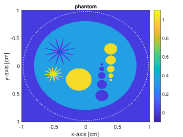
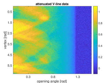
Figure 3.1: Phantom and noisy data used for the numerical results. Left: The numerical phantom $f\in{\boldsymbol{f}}\in\mathbb{R}^{257\times 257}$ consists of the superposition of ellipse and two star shaped tumor like structures. Right: Simulated data ${\boldsymbol{g}}^{\delta}=\boldsymbol{C}{\boldsymbol{f}}+{\boldsymbol{\xi}}\in\mathbb{R}^{200\times 151}$ with $5\%$ noise added.

Discrete forward and adjoint operator

The discrete forward and adjoint operators are defined by considering the entries ${\boldsymbol{f}}[i_{1},i_{2}]$ as sampled values of a function $f$ at locations $(-1,-1)+2(i_{1},i_{2})/N$ for $(i_{1},i_{2})\in\{0,\dots,N\}^{2}$ and replacing the function $f$ by a bilinear interpolant $T[{\boldsymbol{f}}]$. The attenuated V-line transform $\boldsymbol{C}{\boldsymbol{f}}={\boldsymbol{g}}$ is discretized by numerically computing the integral of the interpolant $T[{\boldsymbol{f}}]$ over each of the two branches of the V-lines with the composite trapezoidal rule. We take $(\cos(\varphi[k]),\sin(\varphi[k]))$ with $\varphi[k]=2\pi(k-1)/P$ for $k\in\{1,\dots,P\}$ for the vertex positions, and $\psi[\ell]=\pi\,\ell/(2Q)$ with $\ell\in\{0,\dots,Q\}$ for the opening angles. For the numerical integration of each branch, we use $N+1$ equidistant radii in the interval $[0,2]$. The discrete backprojection operator is defined by using the trapezoidal rule similar to the well-known approach for the classical Radon transform [43].

For the following numerical results we use $N=256$, $P=200$, $Q=150$, and $\mu=0.5$. The used discrete phantom ${\boldsymbol{f}}$ and the numerically computed data $\boldsymbol{C}{\boldsymbol{f}}$ with added Gaussian noise are shown in Figure 3.1.

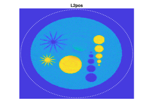
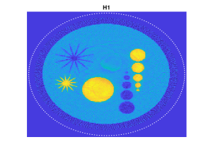
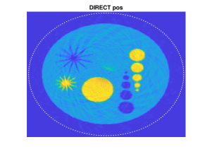
Figure 3.2: Reconstructions from exact data. Top left: least squares. Top right: positivity constraint least squares. Line 2, left: $L^{2}$-regularization. Line 2, right: $L^{2}$-regularization with positivity constraint. Line 3, left: $H^{1}$-regularization. Line 3, right: $H^{1}$-regularization with positivity constraint. Line 4, left: TV-regularization. Line 4, right: TV-regularization with positivity constraint. Bottom, left: Fourier reconstruction from [20]. Bottom, right: Nonnegative part of Fourier reconstruction.

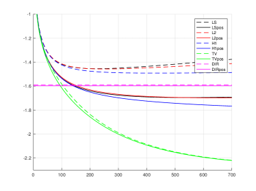
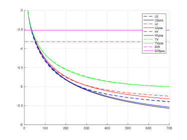
Figure 3.3: Reconstruction errors and residuals from exact data. Left: Logarithm $\log_{10}E^{2}({\boldsymbol{f}}_{j})$ of squared reconstruction error. Right: Logarithm $\log_{10}R^{2}({\boldsymbol{f}}_{j})$ of squared residuals.

Reconstruction from exact data

We first investigate the variational regularization methods on simulated data without noise added. We consider $L^{2}$-regularization, $H^{1}$-regularization and TV-regularization. All methods are used with and without positivity constraint. For comparison purposes, we also perform reconstructions using plain least squares, positivity constrained least squares and the direct Fourier reconstruction method from [20]. The regularization parameter has been taken $\alpha=0.002$ for TV and $H^{1}$ regularization and $\alpha=0.01$ for $L^{2}$ regularization. The reconstruction results after 700 iterations are shown in Figure 3.2. Total variation minimization (with and without positivity constraint) clearly outperforms all other methods. In particular, $L^{2}$- as well as $H^{1}$-regularization contain a ghost source corresponding to the big disc, which is not contained in the TV-reconstruction. Using the least squares methods, the ghost image is also not that severe.

To quantitatively evaluate the reconstructions, we compute the relative squared $\ell^{2}$-error and relative squared $\ell^{2}$-residuals, respectively,

$$E^{2}({\boldsymbol{f}}_{j}) \coloneqq\frac{\sum_{i_{1},i_{2}}\lvert{\boldsymbol{f}}_{j}[i_{1},i_{2}]-{\boldsymbol{f}}[i_{1},i_{2}]\rvert^{2}}{\sum_{i_{1},i_{2}}\lvert{\boldsymbol{f}}[i_{1},i_{2}]\rvert^{2}}$$ (3.4)

$$R^{2}({\boldsymbol{f}}_{j}) \coloneqq\frac{\sum_{k,\ell}\lvert\boldsymbol{C}{\boldsymbol{f}}_{j}[k,\ell]-{\boldsymbol{g}}[k,\ell]\rvert^{2}}{\sum_{k,\ell}\lvert{\boldsymbol{g}}[k,\ell]\rvert^{2}}\,.$$ (3.5)

Logarithmic plots of $E^{2}({\boldsymbol{f}}_{j})$ and $R^{2}({\boldsymbol{f}}_{j})$ are shown in Figure 3.3. The reconstruction error for the TV-regularization is much smaller than for all other methods. The residuals, as expected, are smallest for plain least squares. As a consequence of the ill-posedness, this does not imply small reconstruction error. In fact, the least squares methods show a slight semi-convergence behavior which is due data error introduced by the numerical implementation and the ill-posedness of the inverting the attenuated V-line transform.

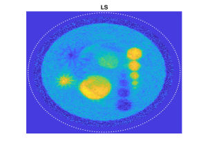
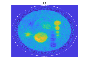
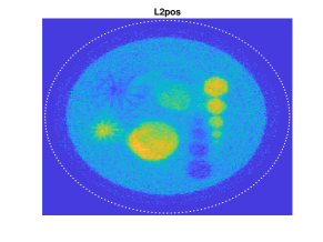
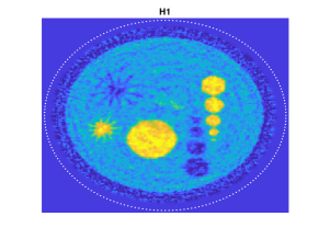
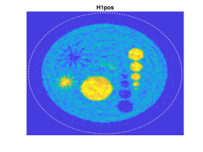
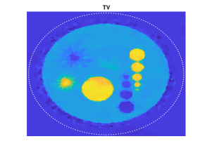
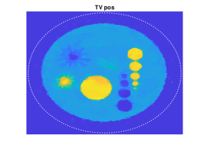
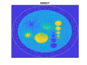
Figure 3.4: Reconstructions from noisy data. Top left: least squares. Top right: positivity constraint least squares. Line 2, left: $L^{2}$-regularization. Line 2, right: $L^{2}$-regularization with positivity constraint. Line 3, left: $H^{1}$-regularization. Line 3, right: $H^{1}$-regularization with positivity constraint. Line 4, left: TV-regularization. Line 4, right: TV-regularization with positivity constraint. Bottom, left: Fourier reconstruction from [20]. Bottom, right: Nonnegative part of Fourier reconstruction.

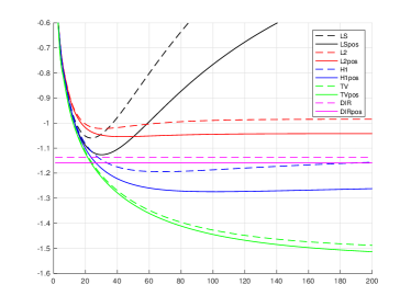
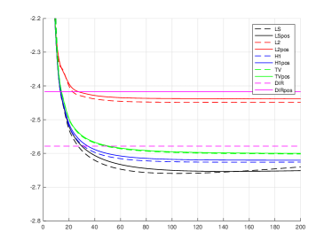
Figure 3.5: Reconstruction errors and residuals from noisy data. Left: Logarithm $\log_{10}E^{2}({\boldsymbol{f}}_{j})$ of squared reconstruction error. Right: Logarithm $\log_{10}R^{2}({\boldsymbol{f}}_{j})$ of squared residuals.

Reconstruction from noisy data

To test the algorithms in a more realistic situation, we repeated the simulation studies where we added additive Gaussian noise ${\boldsymbol{\xi}}\in\mathbb{R}^{(P+1)\times Q}$ to the simulated data. The relative $\ell^{2}$-error

$$\delta=\frac{\sqrt{\sum_{k,\ell}\lvert{\boldsymbol{\xi}}[k,\ell]\rvert^{2}}}{\sqrt{\sum_{k,\ell}\lvert{\boldsymbol{g}}[k,\ell]\rvert^{2}}}$$

is approximately $5\%$. We again consider $L^{2}$-regularization, $H^{1}$-regularization, TV-regularization, least-squares minimization and the Fourier reconstruction method from [20], where each method is used with and without positivity constraint. In order to stabilize the reconstruction, the regularization parameter had to be increased for all methods. It has been taken $\lambda=0.14$ for $L^{2}$-regularization, $\lambda=0.06$ for $H^{1}$-regularization, and $\lambda=0.015$ for TV-regularization.

Reconstruction results from noisy data are shown in Figure 3.4. We used 200 iterations for the regularized iterations and stopped the least squares iterations after 15 iterations in order to prevent overfitting. Logarithmic plots of the squared relative $\ell^{2}$-error $E^{2}({\boldsymbol{f}}_{j})$ and the squared relative $\ell^{2}$-residual $R^{2}({\boldsymbol{f}}_{j})$ are shown in Figure 3.5. As can be seen from the reconstruction as well as the evolution of the reconstruction error, TV-regularization again performs best for the considered type of phantom. In particular, in all other methods, the ghost image is clearly visible and the reconstruction error is much larger than for TV-regularization.

4 Conclusion and outlook

In this paper, we investigated variational regularization methods for the stable inversion of the conical Radon transform with vertices on the sphere. We presented convergence results of variational regularization and a numerical minimization algorithm based on the Chambolle-Pock primal dual algorithm [37, 42]. In particular, the algorithm framework allows a TV-regularizer, quadratic penalties, positivity constraint as well as their combinations. In terms of relative $\ell^{2}$-reconstruction error, we found TV-regularization to clearly outperform least squares quadratic-regularization (all with or without positivity constraint).

The results in this paper show that compared to quadratic regularization, the use of non-smooth convex regularization can clearly improve reconstruction of the conical Radon transforms. Several interesting generalizations of variational regularization are possible. First, one could replace the sphere with more general surfaces of vertices and allow different axis for each vertex location. Second, the algorithmic framework can be extended to variable axis on the sphere. The transform then depends on the $2n-1$ independent variables and is therefore highly overdetermined. In applications such as emission tomography with Compton camera, the noise level is usually high and the full overdetermined transform must actually be used for image reconstruction. Moreover, noise statistics as well as factors governing system performance such as Doppler broadening or polarization [22] should be included in the forward and adjoint problem. Resulting algorithms based on conical Radon transforms (which require binning of Compton camera raw data) should be compared with list mode EM reconstruction algorithms [44] that work without data binning.

Besides numerical investigations, several theoretical aspects have to be addressed in future work. This includes stability and uniqueness analysis as well as range descriptions of the various forms of conical Radon transforms.

References

- Allmaras et al. [2013] M. Allmaras, D. Darrow, Y. Hristova, G. Kanschat, and P. Kuchment. Detecting small low emission radiating sources. Inverse Probl. Imaging, 7(1):47–79, 2013.
- Maxim et al. [2009] V. Maxim, M. Frandes, and R. Prost. Analytical inversion of the Compton transform using the full set of available projections. Inverse Problems, 25(9):1–21, 2009.
- Palamodov [2017] V. Palamodov. Reconstruction from cone integral transforms. Inverse Problems, 33(10):104001, 2017.
- Ambartsoumian and Roy [2016] G. Ambartsoumian and S. Roy. Numerical inversion of a broken ray transform arising in single scattering optical tomography. IEEE Trans. Comput. Imaging, 2(2):166–173, 2016.
- Cree and Bones [1994] M. J. Cree and P. J. Bones. Towards direct reconstruction from a gamma camera based on compton scattering. IEEE Trans. Med. Imaging, 13(2):398–407, 1994. ISSN 0278-0062.
- Haltmeier [2014] M. Haltmeier. Exact reconstruction formulas for a radon transform over cones. Inverse Problems, 30(3), 2014.
- Basko et al. [1998] R. Basko, G. L. Zeng, and G. T. Gullberg. Application of spherical harmonics to image reconstruction for the compton camera. Phys. Med. Biol., 43(4):887, 1998.
- Gouia-Zarrad and Ambartsoumian [2014] R. Gouia-Zarrad and G. Ambartsoumian. Exact inversion of the conical radon transform with a fixed opening angle. Inverse Problems, 30(4):045007, 2014.
- Jung and Moon [2015] C. Jung and S. Moon. Inversion formulas for cone transforms arising in application of Compton cameras. Inverse Problems, 31(1):015006, 20, 2015.
- Parra [2000] L. C. Parra. Reconstruction of cone-beam projections from compton scattered data. IEEE Trans. Nucl. Sci., 47(4):1543–1550, 2000. ISSN 0018-9499.
- Smith [2005] B. Smith. Reconstruction methods and completeness conditions for two compton data models. J. Opt. Soc. Am. A, 22(3):445–459, 2005.
- Kuchment and Terzioglu [2016] P. Kuchment and F. Terzioglu. Three-dimensional image reconstruction from compton camera data. SIAM J. Imaging Sci., 9(4):1708–1725, 2016.
- Tomitani and Hirasawa [2002] T. Tomitani and M. Hirasawa. Image reconstruction from limited angle compton camera data. Phys. Med. Biol., 47(12):2129, 2002.
- Maxim [2014] V. Maxim. Filtered backprojection reconstruction and redundancy in compton camera imaging. IEEE Tran. Image Process., 23(1):332–341, 2014.
- Morvidone et al. [2010] M. Morvidone, M. K. Nguyen, T. T. Truong, and H. Zaidi. On the V-line Radon transform and its imaging applications. Int. J. Biomed. Imaging, 2010:208179, 6, 2010.
- Terzioglu et al. [2018] F. Terzioglu, P. Kuchment, and L. Kunyansky. Compton camera imaging and the cone transform: a brief overview. Inverse Problems, 34(5):054002, 2018.
- Moon and Haltmeier [2017] S. Moon and M. Haltmeier. Analytic inversion of a conical radon transform arising in application of compton cameras on the cylinder. SIAM J. Imaging Sci., 10(2):535–557, 2017.
- Smith [2011] B. D. Smith. Line-reconstruction from compton cameras: data sets and a camera design. Optical Engineering, 50(5):053204, 2011.
- Schiefeneder and Haltmeier [2017] D. Schiefeneder and M. Haltmeier. The radon transform over cones with vertices on the sphere and orthogonal axes. SIAM J. Appl. Math., 77(4):1335–1351, 2017.
- Haltmeier et al. [2017a] M. Haltmeier, S. Moon, and D. Schiefeneder. Inversion of the attenuated v-line transform with vertices on the circle. IEEE Trans. Comput. Imaging, 3(4):853–863, 2017a.
- Zhang [2018] Y. Zhang. Artifacts in the inversion of the broken ray transform in the plane, 2018. arXiv:1711.08575.
- Rogers et al. [2004] W. L. Rogers, N. H. Clinthorne, and A. Bolozdynya. Compton cameras for nuclear medical imaging. In Emission Tomography: The Fundamentals of PET and SPECT, pages 383–419. Elsevier, 2004.
- Todd et al. [1974] R. W. Todd, J. M. Nightingale, and D. B. Everett. A proposed gamma camera. Nature, 251:132–134, 1974.
- Florescu et al. [2011] L. Florescu, V. A. Markel, and J. C. Schotland. Inversion formulas for the broken-ray radon transform. Inverse Problems, 27(2):025002, 2011.
- Bellini et al. [1979] S. Bellini, M. Piacentini, C. Cafforio, and F. Rocca. Compensation of tissue absorption in emission tomography. IEEE Trans. Acoust., Speech, Signal Processing, 27(3):213–218, 1979. doi: 10.1109/TASSP.1979.1163232.
- Novikov [2002] R. G. Novikov. An inversion formula for the attenuated x-ray transformation. Arkiv för matematik, 40(1):145–167, 2002.
- Hawkins et al. [1988] W. G. Hawkins, P. K. Leichner, and N.-C. Yang. The circular harmonic transform for spect reconstruction and boundary conditions on the fourier transform of the sinogram. IEEE Trans. Med. Imag., 7(2):135–138, 1988.
- Inouye et al. [1989] T. Inouye, K. Kose, and A. Hasegawa. Image reconstruction algorithm for single-photon-emission computed tomography with uniform attenuation. Physics in Medicine and Biology, 34(3):299–304, 1989.
- Puro [2001] A. Puro. Cormack-type inversion of exponential Radon transform. Inverse Problems, 17(1):179, 2001.
- Tretiak and Metz [1980] O. Tretiak and C. Metz. The exponential Radon transform. SIAM J. Appl. Math., 39(2):341–354, 1980. doi: 10.1137/0139029.
- Markoe and Quinto [1985] A. Markoe and E. T. Quinto. An elementary proof of local invertibility for generalized and attenuated radon transforms. SIAM journal on mathematical analysis, 16(5):1114–1119, 1985.
- Clough and Barrett [1983] A. V. Clough and H. H Barrett. Attenuated Radon and Abel transforms. J. Opt. Soc. Am., 73(11):1590–1595, 1983.
- Natterer [2001a] F. Natterer. Inversion of the attenuated radon transform. Inverse Problems, 17(1):113, 2001a.
- Kunyansky [2001] L. A. Kunyansky. A new spect reconstruction algorithm based on the novikov explicit inversion formula. Inverse Problems, 17(2):293, 2001.
- Gouia-Zarrad and Moon [(in press] R. Gouia-Zarrad and S. Moon. Inversion of the attenuated conical Radon transform with a fixed opening angle. Math. Method. Appl. Sci., (in press).
- Haltmeier et al. [2017b] M. Haltmeier, S. Moon, and D. Schiefeneder. Inversion of the attenuated v-line transform with vertices on the circle. IEEE Trans. Comput. Imaging, 3(4):853–863, 2017b.
- Chambolle and Pock [2011] A. Chambolle and T. Pock. A first-order primal-dual algorithm for convex problems with applications to imaging. J. Math. Imaging Vision, 40(1):120–145, 2011. ISSN 0924-9907. doi: 10.1007/s10851-010-0251-1. URL http://dx.doi.org/10.1007/s10851-010-0251-1.
- Müller [1966] C. Müller. Spherical Harmonics. Lecture Notes in Mathematics. Springer, Berlin-New York, 1966.
- Seeley [1966] R. T. Seeley. Spherical harmonics. Amer. Math. Monthly, 73(4):115–121, 1966.
- Scherzer et al. [2009] O. Scherzer, M. Grasmair, H. Grossauer, M. Haltmeier, and F. Lenzen. Variational methods in imaging, volume 167 of Applied Mathematical Sciences. Springer, New York, 2009. ISBN 978-0-387-30931-6.
- Combettes and Pesquet [2011] P. L. Combettes and J.-C. Pesquet. Proximal splitting methods in signal processing. In Fixed-point algorithms for inverse problems in science and engineering, pages 185–212. Springer, 2011.
- Sidky et al. [2012] E. Y. Sidky, J. H. Jørgensen, and X. Pan. Convex optimization problem prototyping for image reconstruction in computed tomography with the chambolle–pock algorithm. Phys. Med. Biol., 57(10):3065, 2012.
- Natterer [2001b] F. Natterer. The Mathematics of Computerized Tomography, volume 32 of Classics in Applied Mathematics. SIAM, Philadelphia, 2001b.
- Wilderman et al. [2001] S. J. Wilderman, J. A. Fessler, N. H. Clinthorne, J. W. LeBlanc, and W. L. Rogers. Improved modeling of system response in list mode em reconstruction of compton scatter camera images. IEEE Trans. on Nucl. Sci., 48(1):111–116, 2001.