Synthetic Dimension in Photonics

Abstract

The physics of a photonic structure is commonly described in terms of its apparent geometric dimensionality. On the other hand, with the concept of synthetic dimension, it is in fact possible to explore physics in a space with a dimensionality that is higher as compared to the apparent geometrical dimensionality of the structures. In this review, we discuss the basic concepts of synthetic dimension in photonics, and highlighting the various approaches towards demonstrating such synthetic dimension for fundamental physics and potential applications.

I Introduction

The physics of a photonic structure is commonly described in terms of its apparent geometric dimensionality. A few 0, 1, 2 and 3 dimensional examples are microcavities ward11 ; feng12 , waveguides kawachi90 , two-dimensional photonic crystals joannopoulos97 , and three-dimensional metamaterials soukoulis11 ; liu11 , respectively.

Using these same photonic structures, however, it is in fact possible to explore physics in a space with a dimensionality that is higher as compared to the apparent geometrical dimensionality of these structures. The basic idea is to configure synthetic dimensions, and to combine such synthetic dimensions with the geometric dimensions to form higher dimensional synthetic space regensburger11 ; regensburger12 ; schwartz13 ; luo15 ; yuanol ; ozawa16 .

In photonics, there are two approaches for creating such a synthetic space.

1. Forming a lattice. Consider a system as described by coupling a set of physical states together. The dimensionality of the system is then determined by the nature of coupling. As an illustration, suppose we label the states as consecutive integers, and therefore we can visualize the states as being placed on a line [Fig. 1(a)]. The coupling in Fig. 1(b), where consists of a nearest neighbor coupling between the states, results in a one-dimensional lattice. On the other hand, with the same set of states, one can in fact form higher-dimensional lattices, with the longer-range coupling as indicated in Fig. 1(c).

2. Exploiting the parameter dependency the system. As a general illustration, consider a system in an n-dimensional space, as described by a Hamiltonian of the form $H(p_{1},\ldots,p_{m},r_{1},\ldots,r_{n})$, where $p_{1},\ldots,p_{m}$ are external parameters, and $r_{1},\ldots,r_{n}$ are the spatial coordinates. One can think of each parameter of the Hamiltonian as an extra synthetic dimension.

In additional to photonics, both of these approaches for creating synthetic dimensions have been also extensively explored in other physical systems, such as cold atoms in optical lattices boada12 ; kraus12 ; mei12 ; gomezleon13 ; ganeshan13 ; xu13 ; kraus13 ; celi14 ; mei14 ; boada15 ; price15 ; mancini15 ; stuhl15 ; nakajima16 ; lohse16 ; zeng16 ; suszalski16 ; taddia17 ; price17 ; martin17 ; baum18 ; peng18 ; lohse18 ; shang18 and superconducting qubits strauch08 ; tsomokos10 ; mei16 . The development of the concept of synthetic dimension in photonics share some of the motivations. For examples, theoretically it is known that there are rich physics, and in particular, rich topological physics in systems beyond three dimensions zhang01 ; qi08 ; kitaev09 ; lian16 ; lian17 ; roy17 . The development of synthetic dimension provides an experimental approach to explore such physics. Also, while three dimensional physics can in principle be explored in three dimensional structures, constructing such structures may be challenging and it may be more advantageous to explore such a physics in one or two-dimensional structures that are easier to construct.

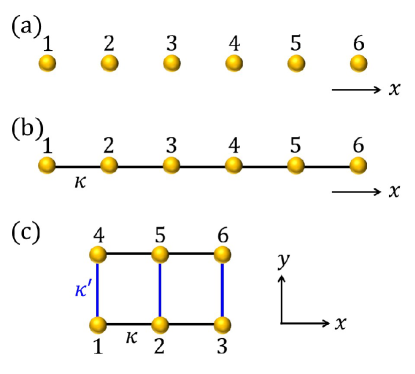
Figure 1: (a) The physical states labelled by consecutive integers. (b) Introducing coupling between nearest-neighbor physical states creates a one-dimensional system. (c) Introducing long-range coupling between different states generates a two-dimensional system schwartz13 ; yuanhaldane .

On the other hand, there are aspects of synthetic dimension concepts that are unique in photonics. In particular, in forming a lattice, the states that are being used can have different frequencies, or different orbital angular momentums, corresponding to different internal degrees of freedom of photons. The construction of the synthetic space thus enables new possibilities for manipulating these internal degrees of freedom, which are of significant potential importance for applications such as communications and information processing.

In this paper, we provide a short review of the current developments of the concepts of synthetic dimension in photonics. The rest of the paper is organized as follows: In Sec. II, we review the approach to create synthetic dimension by designing the coupling between various photonic states to form a synthetic lattice. In Section III, we discuss some of the physics effects in these photonic synthetic lattices, focusing in particular on photonic gauge potential and topological photonics effects. In Sec. IV, we review the approach of exploring high dimensional photonic phenomena in the parameter space. We conclude in Sec. V.

II Forming a synthetic lattice of photonic states

In order to create a synthetic space using the approach of forming a lattice, one needs a set of physical states, as well as mechanisms to specifically configure the coupling among these states. Photonics offers a rich variety of possibilities for forming lattices. For the states, one can use photonic modes with different frequencies, or with different spatial distributions such as different orbital angular momentums, or alternatively one can use multiple temporal pulses. Photonic structures also offer great flexibilities in configuring the coupling of these different states. In this section, we brief review these various approaches for creating synethic space by forming a lattice.

II.1 Using photonic modes with different frequencies

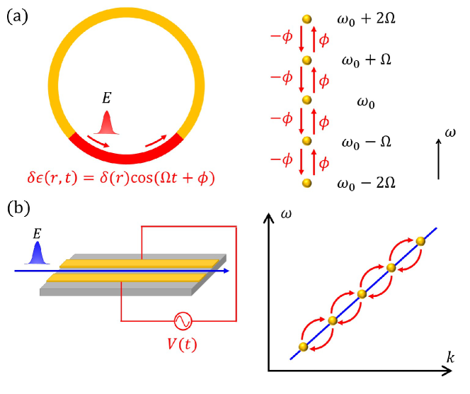
Figure 2: (a) A dynamically modulated ring resonator can be described by a tight-binding model of a photon along a one-dimensional lattice in the synthetic frequency dimension yuanol ; yuanoptica . (b) A phase-matched modulation along a dielectric waveguide can achieve a one-dimensional lattice formed from waveguide modes at different frequencies qin18 ; bell17 .

In photonics, a natural way to create a synthetic dimension is to use the frequency of light. Photonic structures naturally support modes at different frequencies. Moreover, a lattice can be formed by coupling these modes together, through either dynamic modulation of the structure, or by nonlinear optics techniques.

As a simple illustration of the use of dynamic modulation to couple modes with different frequencies together, consider a structure with a time-dependent permittivity described by:

$$\epsilon(r,t)=\epsilon_{s}(r)+\delta\epsilon(r,t),$$ (1)

where $\epsilon_{s}(r)$ describes a static dielectric structure, and $\delta\epsilon(r,t)$ describes a time-dependent modulation. For such a time-dependent system, its electromagnetic properties can be described from the Maxwell’s equation as:

$$\nabla\times\nabla\times E+\mu_{0}\frac{\partial^{2}}{\partial t^{2}}\epsilon_{s}E=-\mu_{0}\frac{\partial^{2}P}{\partial t^{2}},$$ (2)

where

$$P=\delta\epsilon E$$ (3)

is the polarization current density induced by the dynamic modulation.

Since for typical modulation, we have $|\delta\epsilon|\ll\epsilon_{s}$, one can treat the dynamically modulated structure perturbatively. We first determine the mode of the static structure by solving an eigenvalue problem:

$$\nabla\times\nabla\times E_{m}=\mu_{0}\epsilon_{s}\omega_{m}^{2}E_{m},$$ (4)

where $\omega_{m}$ is the frequency of the mode, and $E_{m}$ is the eigenmode field distribution. For the dynamic structure, the modulation induces coupling between these modes. Therefore, we expand the field $E$ in terms of the eigenmodes of the static structure:

$$E=\sum_{m}a_{m}E_{m}e^{i\omega_{m}t},$$ (5)

and describe the properties of the dynamic structure in terms of the dynamics of the modal amplitudes $a_{m}$${}^{\prime}s$.

The formalism above can be used to describe a modulated ring resonator yuanol ; ozawa16 ; yuanoptica ; linnc ; zhang17 ; yuanhaldane ; lin18 ; yuanPT . Consider a static ring resonator composed of a single-mode waveguide, which we assume to have zero group velocity dispersion for simplicity. Suppose the ring supports a resonant mode at a frequency $\omega_{0}$. In the vicinity of the frequency $\omega_{0}$, resonant modes then form an equally spaced frequency comb, with the $m$-th resonant mode having the frequency

$$\omega_{m}=\omega_{0}+m\Omega_{R}.$$ (6)

In Eq. (6), $\Omega_{R}=2\pi c/n_{0}L$ is the free-spectral range of the ring which also defines the modal spacing in frequency, $n_{0}=n(\omega_{0})$ is the group index of the waveguide at $\omega_{0}$, and $L$ is the circumference for the ring.

Suppose we modulate the ring resonator structure above as:

$$\delta\epsilon(r,t)=\delta(r)\cos(\Omega t+\phi),$$ (7)

where $\delta(r)$ is the modulation profile, $\Omega$ is the modulation frequency and $\phi$ is the modulation phase. For simplicity we set $\Omega=\Omega_{R}$. The induced polarization density from the $m$-th mode is then

$$P=\frac{\delta(r)E_{m}}{2}a_{m}\left(e^{i\phi}e^{i\omega_{m+1}t}+e^{-i\phi}e^{i\omega_{m-1}t}\right).$$ (8)

Thus, the induced polarization will resonantly excite modes $m+1$ and $m-1$. Hence we expect that the modal amplitudes satisfies:

$$i\frac{da_{m}}{dt}=ge^{i\phi}a_{m-1}+ge^{-i\phi}a_{m+1}.$$ (9)

Here $g$ is the coupling strength. (A detailed derivation can be found in Refs. yuanol ; ozawa16 .) The Hamiltonian of such a system is then

$$H=g\sum_{m}\left(e^{i\phi}c^{\dagger}_{m+1}c_{m}+e^{-i\phi}c^{\dagger}_{m}c_{m+1}\right).$$ (10)

where $c_{m}(c^{\dagger}_{m})$ is the annihilation (creation) operator for the $m$-th resonant mode. The Hamiltonian in Eq. (10) describes a tight-binding model of a photon in a one-dimensional lattice in the synthetic frequency dimension yuanol ; yuanoptica .

Similar approach for creating a synthetic dimension along the frequency axis can also be achieved in a waveguide. Consider a static single-mode waveguide with the propagation direction along the $z$-direction, its eigenmode has the form

$$E_{k}=E_{k}(x,y)e^{-ikz}.$$ (11)

Here $E_{k}(x,y)$ is the modal profile, and $k$ is the wavevector. The eigenfrequency of the mode is $\omega(k)$, which also defines the dispersion relation of the waveguide. Suppose we operate in the vicinity of an operating frequency $\omega_{0}$ with the corresponding wavevector $k_{0}$, i.e. $\omega_{0}=\omega(k_{0})$. Near $\omega_{0}$ one can expand the dispersion relation as:

$$\omega-\omega_{0}=v_{g}(k-k_{0}),$$ (12)

where $v_{g}$ is the group velocity of the waveguide.

For such a waveguide, we then modulate its permittivity as:

$$\delta\epsilon=\delta(x,y)\cos(\Omega t-Kz+\phi),$$ (13)

where we choose the modulation to be phase-matched with the waveguide mode, such that

$$\Omega=Kv_{g},$$ (14)

In the presence of such modulation, we expand the field in the waveguide as:

$$E=\sum_{m}a_{m}(z)E_{m}(x,y)e^{i\left(\omega_{m}t-k_{m}z\right)},$$ (15)

where $\omega_{m}=\omega_{0}+m\Omega$, and $k_{m}$ is the corresponding wavevector, i.e. $\omega_{m}=\omega(k_{m})$. The induced polarization from the $m$-th mode has the form

$$P=\frac{\delta(x,y)E_{m}(x,y)}{2}a_{m}\left[e^{i\phi}e^{i\left(\omega_{m+1}t-k_{m+1}z\right)}+e^{-i\phi}e^{i\left(\omega_{m-1}t-k_{m-1}z\right)}\right],$$ (16)

We see that the induced polarization would couple with the $m+1$ and $m-1$ mode in a phase-matched fashion. We expect that the coupled mode theory to have the form:

$$i\frac{da_{m}}{dz}=ge^{i\phi}a_{m-1}+ge^{-i\phi}a_{m+1}.$$ (17)

We again see a one-dimensional tight binding model for photons along a synthetic frequency dimension.

The modulations in Eqs. (7) and (13) can be achieved using electro-optical modulation qin18 . Recent developments of on-chip silicon tzuang14 and LiNbO₃ modulators wang14nb ; zhang17nb in either ring resonator or waveguide geometries may prove to be quite useful for creating synthetic lattice. In addition, one can also consider the use of accoustic-optical modulators in fiber ring resonators. Similar effects can also be accomplished with the use of nonlinear optical effects peschel08 ; bersch09 . Ref. bell17 used two strong pumps differ in frequency by $\Omega$, to create a synthetic lattice along the frequency dimension, for a weak probe wave. Similar four-wave mixing process has also been considered in a Raman medium yuanraman .

II.2 Using photonic modes with different orbital angular momentum

Instead of creating a synthetic dimension in the spectral domain, one can also create a synthetic dimension exploiting the spatial degree of freedom in optical modes. Consider a light beam, with its transverse profile carrying non-zero orbital angular momentum, circulating around in a ring cavity to form resonant modes of the cavity. In general, the resonant frequency of such a resonant mode should depend on the orbital angular momentum of the corresponding circulating beam. However, with appropriate design, one can in fact create a degenerate optical cavity, in which resonant modes formed by beams with different orbital angular momenta have the same frequency. Inside such degenerate cavity, one can then introduce an auxiliary cavity, which incorporates spatial light modulators, in order to couple a small portion of the amplitude of a beam with an orbital angular moment $l$ to a beam with an orbital angular moment $l-1$ and $l+1$. The system then is described by a tight-binding model luo15 ; luo17 ; sun17 ; zhou17 ; luo18

$$H=g\sum_{l}\left(e^{i\phi}c^{\dagger}_{l}c_{l-1}+e^{-i\phi}c^{\dagger}_{l}c_{l+1}\right),$$ (18)

where $l$ corresponds to the orbital angular moment of light. Thus, the cavity structure shown in Fig. 3 can be used to achieve a synthetic dimension based on the orbital angular momentum. While here for simplicity we consider only nearest neighbor coupling along the $l$-axis, long-range coupling can also be achieved with different design of the spatial light modulators (Ref. luo17 ).

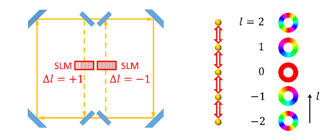
Figure 3: A cavity that is degenerate for optical beams with different angular momentum (solid line). Within this cavity, an auxiliary cavity (dashed line) is incorporated, where two spatial light modulators couple a beam at angular momentum $l$ to beams at angular momentums $l\pm 1$, respectively. Such a cavity can be described by a synthetic lattice along the angular momenta direction luo15 .

II.3 Using multiple pulses

Another platform to create a synthetic photonic lattice is to exploit the temporal degree of freedom, where the evolution of a sequence of pulses is mapped onto the dynamics of a particle moving on a set of discrete lattice sites regensburger11 ; regensburger12 ; wimmer13 ; regensburger13 ; wimmer15 ; wimmer17 ; vatnik17 ; wimmer18 . As an illustration, consider two fibre loops with different lengths, connected by a $50/50$ coupler [see Fig. 4(a)]. We assume that the round-trip times for light travelling through the short and long loops are $T_{s}$ and $T_{l}$, respectively, with the time difference $T_{l}-T_{s}\equiv 2\Delta T$ and the average time $(T_{l}+T_{s})/2\equiv T$. Within the long loop there is in addition a phase modulator. For a pulse at a particular position in the short (long) loop at the time $t_{0}$, after a round trip around the short (long) trip, it returns to the same position at the time $t_{0}+T-\Delta T$ ($t_{0}+T+\Delta T$). Suppose at the time $t=mT+n\Delta T$, two pulses, denoted as $u_{n}^{m}$ and $v_{n}^{m}$, arrives at the input ends of the coupler in the short and long loops, respectively. Two pulses $u^{m}_{n+1}$ and $v^{m}_{n+1}$, upon passing through the coupler, generates an output pulse in the short loop. Such an output pulse then goes through a round trip in the short loop to generate $u^{m+1}_{n}$, i.e.

$$u_{n}^{m+1}=\frac{1}{\sqrt{2}}\left(u^{m}_{n+1}+iv^{m}_{n+1}\right).$$ (19)

And similarly

$$v_{n}^{m+1}=\frac{1}{\sqrt{2}}\left(iu^{m}_{n-1}+v^{m}_{n-1}\right)e^{i\phi(n)},$$ (20)

In Eqs. (19) and (20), we have used the scattering matrix of the coupler, and have incorporated the effects of the phase modulators. Here we assume that the modulation period is $T$, and hence the time-dependent transmission phase depends on $n$ only. Eqs. (19) and (20) describe the temporal motion (motion along the $m$-axis) of a particle on a one-dimensional synthetic lattice as labelled by $n$.

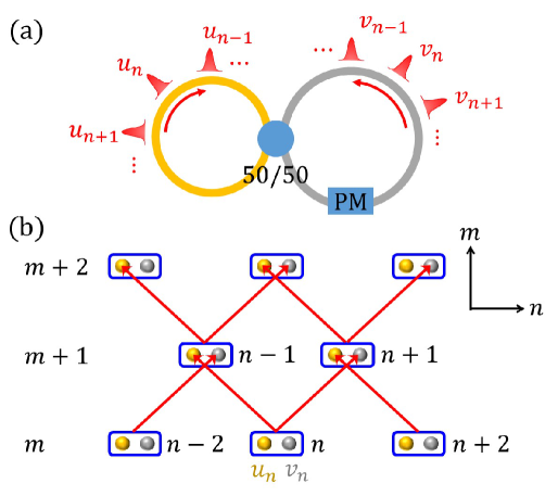
Figure 4: (a) Two fibre loops connected by a $50/50$ coupler. (b) An equivalent lattice network which describes a one-dimensional synthetic lattice ($n$) evolves along the time ($m$) regensburger11 ; regensburger12 .

To summarize Section II, photonics provides a rich set of opportunities to create synthetic lattices. The general idea here is to specifically design the coupling between various photonic modes. In addition to the few examples above, with different spectral, spatial and temporal modes, there exist many other possibilities of utilizing photonic modes. For example, Ref. lustig18 experimentally demonstrated a synthetic lattice that maps into a topological insulator, based on modes in an array of coupled waveguides. While in the examples above for simplicity we have considered one-dimensional synthetic lattices with nearest neighbor coupling, it is possible to achieve higher dimensional synthetic lattice with more complex couplings. For example, Refs. schwartz13 ; yuanhaldane show that by utilizing modulators with a few modulation frequencies, one can achieve a synthetic lattice with dimensions higher than one using the same set of modes in the ring resonator here as we considered in Section II. A. The effects of long-range coupling in synthetic dimensions have been also explored in Ref. bell17 .

In photonics, the number of distinct lattice sites along the synthetic dimension can potentially be quite large. For ring resonators systems, for example, it is conceivable to have hundreds of different modes coupling together, since the modulation frequency is typically far smaller than the resonant frequencies of the modes. Have such a large space along the synthetic dimension is useful for the demonstration of analogues of bulk physics effects in the synthetic space. In addition, the boundaries along the synthetic dimension can also be introduced, either naturally through the group velocity dispersion for the modulated ring or waveguides yuanol , or by specifically designed boundaries using a memory effect baum18 .

III The Physics of Synthetic Lattice

The photonic synthetic lattices as discussed in Section II provide versatile platforms to explore fundamental physics effects. In addition, since the synthetic lattice is built upon various degrees of freedom of light, the abilities to control the flow of light in the synthetic lattice provides abilities to control properties of light that are important for practical applications.

The description of a dynamically modulated ring in terms of a one-dimensional tight-binding model certainly has a long history. This description, for example, has been used to described the physics of mode-locked lasers harris65 ; harris67 ; haus75 ; haus00 . In recent years, the concept of the synthetic lattice has been explored to demonstrate a wide range of physics effects including the physics of parity-time symmetry regensburger12 ; regensburger13 ; wimmer15 ; yuanPT , Anderson localization vatnik17 , and time-reversal of light wimmer18 . Here we focus on two important emerging directions in the physics of synthetic lattice: creating an effective gauge potential for light, and topological photonics effects.

III.1 Effective gauge potential

Photons are neutral particles. Thus, there is no naturally occurring gauge potential that couples to photons. On the other hand, in the construction of photonic synthetic lattices, the ability for achieving an effective gauge potential for photons naturally emerge. To illustrate the concept of such an effective gauge potential for photons fang12 ; fang12np ; yuanprl , consider first the Hamiltonian

$$H=g\sum_{\langle i,j\rangle}\left(e^{-i\phi_{ij}(t)}c_{i}^{\dagger}c_{j}+e^{i\phi_{ij}(t)}c_{j}^{\dagger}c_{i}\right),$$ (21)

where $\phi_{ij}(t)$ is the hopping phase between lattice sites $i$ and $j$. The hopping phase in general can be time-dependent. For simplicity we consider only nearest neighbor coupling. We can therefore make the association luttinger51

$$\int_{i}^{j}A\cdot d\mathbf{r}=\phi_{ij}(t).$$ (22)

where $A$ is the effective gauge potential for photons. In a higher dimensional lattice fang12np ,

$$B=\frac{1}{S}\oint_{\mathrm{plaquette}}A\cdot d\mathbf{r}$$ (23)

is the effective magnetic field through a plaquette, here $S$ is the area of the plaquette. Also, if $\phi_{ij}(t)$ is time dependent, we then have a time dependent gauge potential $A(t)$ yuanprl .

$$E=-\frac{\partial A}{\partial t}$$ (24)

is therefore an effective electric field for photons. As we see in Section II, the various techniques for creating a photonic synthetic lattice naturally incorporates the capabilities for controlling such hopping phases in the lattice. Therefore, these technique naturally leads to gauge potentials, as well as effective electric or magnetic fields for photons.

As perhaps the simplest illustration of the effect of a gauge potential, we consider the effect of Bloch oscillation in the synthetic space along the frequency axis. Bloch oscillation occurs when a charge particle in a one-dimensional lattice is subject to a constant electric field. This effect, initially proposed in solid state physics bloch29 , has been previously considered for photons in waveguide arrays lenz99 ; trompeter06 ; longhi06 ; dreisow09 ; levy10 and photonic crystals kavokin00 ; malpuech01 ; sapienza03 ; agarwal04 ; lousse05 ; estevez15 . Here we show that such an effect can occur in the synthetic space as well yuanoptica ; longhi05 ; bersch09 ; peschel08 ; bersch11 . Consider the ring resonator incorporating a phase modulator as discussed in Section II. A. By choosing the modulation frequency $\Omega$ to be slightly different from the mode spacing $\Omega_{R}$, the resulting Hamiltonian has the same form as Eq. (10), but with a time-dependent phase $\phi(t)=(\Omega-\Omega_{R})t$. From Eq. (24), then, such a modulation results in an effective time-independent electric field in the synthetic space.

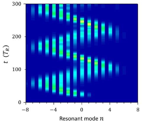
Figure 5: The evolution of the light in time for each resonant mode $n$ exhibits the spectral Bloch oscillation yuanoptica .

The effect of such a constant effective electric field can be seen in Fig. 5. Suppose at $t=0$ a few spectral components are excited. As time evolves the excited spectral components oscillates, which is precisely the effect of Bloch oscillation in the spectral domain. Moreover, it was noted in Ref. yuanoptica that a periodic switching of the modulation frequency around the mode spacing can give rise to a uni-directional shift of photons along the frequency axis, which is a useful capability for controlling the frequency of light. Related capabilities for controlling the spectrum of light, including negative refraction and focusing of light along the frequency axis, has also been demonstrated by creating a photonic gauge potential in a waveguide bell17 ; peschel08 ; bersch09 ; qin18 , based on the waveguide system as discussed in Section II. A.

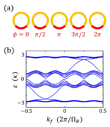
Figure 6: (a) A one-dimensional array of ring resonators undergoing dynamic modulations yuanol ; ozawa16 . The modulators in the rings have different modulation phases $\phi$. (b) Projected band structure for the system in (a) with 21 rings, assuming that the lattice is infinite along the synthetic frequency dimension yuanol .

One can also explore the consequences of effective magnetic fields for photons in the synthetic space yuanol ; ozawa16 ; yuanraman . For this purpose, consider an array of identical ring resonators, each of which incorporates a phase modulator with the modulation frequency equal to the mode spacing in the ring [Fig. 6(a)]. Based on the discussion in Section II. A, each ring supports a one-dimensional lattice along the frequency axis. The modes in nearest-neighbor rings at the same frequency are also coupled through evanescent tunnelling. The system thus is described by a Hamiltonian:

$$H=\sum_{m,n}g\left(e^{-in\phi}c^{\dagger}_{m,n}c_{m+1,n}+e^{in\phi}c^{\dagger}_{m+1,n}c_{m,n}\right)+\kappa\left(c^{\dagger}_{m,n}c_{m,n+1}+c^{\dagger}_{m,n+1}c_{m,n}\right),$$ (25)

where $m$ denotes the different modes in the same ring, $n$ labels a ring in the array, and $\kappa$ is the coupling constant due to evanescent tunnelling between two nearest-neighbor rings. We assume that the spacing between the rings is $d$. By choosing the modulation phase in Eq. (7) to be $n\phi$ for the modulator in the $n$-th ring, as shown in Eq. (25), the resulting Hamiltonian gives rise to a uniform effective magnetic field $\phi/\Omega_{R}d$ in the synthetic space as described in the Landau gauge.

The Hamiltonian of Eq. (25) is periodic along the frequency axis (i.e. $m$-axis). Thus the wavevector reciprocal to the frequency axis, $k_{f}\in[-\pi/\Omega_{R},\pi/\Omega_{R})$, is conserved. Such $k_{f}$ conservation remains true even with a finite number of rings. In Fig. 6(b), we plot the projected bandstructure, which represents the eigenvalues of the Hamiltonian in Eq. (25) as a function of $k_{f}$, for a system consisting of 21 rings with the choice of $\phi=\pi/2$ yuanol . The bandstructure exhibits one-way edge states, as expected for such a lattice system in the presence of an effective magnetic field. This system therefore enables one-way frequency translation that is topologically protected. Hamiltonian similar to Eq. (25) can also be created in the synthetic space based on orbital angular momentum of light as discussed in Section II. B luo15 . In such a case the system provides a novel platform for controlling and converting the orbital angular moment of light, which is of potential importance for communication applications.

III.2 Topological Photonics

In the previous section, the Hamiltonian of Eq. (25) in fact is topologically non-trivial. The resulting band structure has non-trivial Chern number that arises from the effective magnetic field. In addition to using such magnetic field, there are other mechanisms in the synthetic systems to achieve non-trivial topological effects. For example, in a system similar to what has been discussed in Section II. B, where modes with different orbital angular momenta are coupled together to form a one-dimensional synthetic lattice, one can realize the Su-Schriffer-Heeger (SSH) model with a sharp boundary, and hence demonstrating bulk-edge correspondence in the SSH model zhou17 .

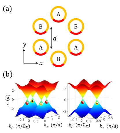
Figure 7: (a) A two-dimensional honeycomb array of ring resonators undergoing dynamic modulations. (b) Bandstructures show Weyl points in three-dimensional synthetic space. Left (right): the band structure in $k_{x}(k_{y})-k_{f}$ plane at $k_{y}=0$ ($k_{x}=4\pi/3\sqrt{3}d$) linnc .

The effects of topological physics depends strongly on the dimensionality of the physical system. There are rich set of effects that are unique to higher-dimensional system with no lower-dimensional counterparts. The concept of synthetic dimension provides a natural pathway towards exploring these higher-dimensional physics.

Here we illustrate this pathway by considering the exploration of Weyl point physics in synthetic dimension linnc ; zhang17 ; sun17 . A Weyl point is a two-fold degeneracy in a three-dimensional band structure with linear dispersion in its vicinity weyl29 . The Weyl point is of substantial interest in topological physics because it represents a magnetic monopole in the momentum space, and hence its presence is robust to any small perturbation.

Photonic structures that support a Weyl point typically have complex three-dimensional geometries bravoabad15 ; lu15 ; chen15 ; wang16weyl . On the other hand, with the concept of synthetic dimension, it is in fact possible to explore Weyl-point physics with two-dimensional geometries that are easier to construct. Consider a two-dimensional array of ring resonators forming a honeycomb lattice. Each ring resonator incorporates a phase modulator. Therefore, as discussed in Section II. A, each ring supports a one-dimensional lattice along the frequency axis. The system thus is described by a three-dimensional lattice model. It was shown in Ref. linnc that Weyl-point physics emerges by appropriately choosing the modulation phases $\phi_{A}$ and $\phi_{B}$, on the $A$ and $B$ sites of the honeycomb lattices (Fig. 7). Along similar directions, Ref. lin18 showed that a three-dimensional topological insulator can be constructed using a two-dimensional ring resonator lattice. Four-dimensional quantum Hall effect has been studied in a three-dimensional resonator lattice ozawa16 . Also, it was shown that the two-dimensional Haldane model can be implemented using only three ring resonators yuanhaldane .

In Section II we have discussed various techniques for achieving long-range coupling in the synthetic space. Such long range coupling can be used to create topological flat bands sun11 ; tang11 which is important for simulating of many-body physics including the fractional quantum Hall effect umucalilar12 . The presence of long-range coupling can also be used for achieving novel band structure effects such as a single Dirac cone in a two-dimensional system without breaking time-reversal symmetry mross16 .

Exploration of nonlinear effects in synthetic space is certainly of fundamental interests in the context, for example, of quantum simulations. In many important interacting lattice Hamiltonians, the interaction is local with respect to the lattice sites. On the other hand, for the schemes involving the frequency axis as the synthetic dimension, typical nonlinear optics effects result in a form of interaction that is nonlocal across different lattice sites strekalov16 , and thus is not directly suitable for the simulation of local-interacting Hamiltonians. Ref. ozawa17 proposed to achieve local interaction in a system where the synthetic dimension is the geometrical angular coordinate. It is an interesting open question to achieve local interaction for other approaches aiming to create synthetic space.

IV Synthetic dimension from parameter space

IV.1 Physics concept

Instead of forming a synthetic lattice, another common method to create a synthetic space is to utilize the parameter degrees of freedom. Consider any physical system as described by a Hamiltonian $H(p)$ that is parametrically dependent on a continuous variable $p$. The parameter dependency of the system can be alternatively described in a synthetic space with the $p$-axis as an extra synthetic dimension in addition to the usual physical space. In this way, higher dimensional physics can then manifest in terms of parameter dependency of a lower-dimensional physical system.

The concept of gauge potential and the associated topological physics effects naturally arise in such synthetic space incorporating the parameter axis. As a simple illustration, consider a Hamiltonian in the parameter space described by a two-dimensional vector $\mathbf{R}$, which satisfies the Schrödinger equation berry84 ; raffaele00

$$H(\mathbf{R})|\Psi(\mathbf{R})\rangle=E(\mathbf{R})|\Psi(\mathbf{R})\rangle,$$ (26)

We assume that as $\mathbf{R}$ varies the Hilbert space does not change. Suppose we consider a closed curve $\mathcal{C}$ in the $R$-space. Along this closed loop, one can define the Berry’s phase $\gamma$ as

$$\gamma=\oint_{\mathcal{C}}i\langle\Psi(\mathbf{R})|\nabla_{\mathbf{R}}|\Psi(\mathbf{R})\rangle\cdot d\mathbf{R}.$$ (27)

The integral kernel here gives the Berry connection, or the gauge potential in parameter space:

$$\mathbf{A}(\mathbf{R})=i\langle\Psi(\mathbf{R})|\nabla_{\mathbf{R}}|\Psi(\mathbf{R})\rangle.$$ (28)

With the Stokes’s theorem, we obtain the Berry curvature

$$\mathbf{B}(\mathbf{R})=\nabla_{\mathbf{R}}\times\mathbf{A}(\mathbf{R}).$$ (29)

The usual topological description of a two-dimensional band structure can be formulated in exactly the same fashion as above, with $\mathbf{R}$ corresponding to the wavevector $k$ roushan14 ; schroer14 ; yale16 . Since the wavevector is defined on the first Brillouin zone which is a 2-torus, the integration of the $B$-field is quantized and gives rise to the Chern numbers of the bands. The important observation here, however, is that the topological argument commonly used for band-structure can in fact be used for any parameter dependency. Moreover, if one were to vary the parameter as a function of time adiabatically, the dynamics of such time-dependent system has signature of higher dimensional topological physics. Below, we illustrate these aspects with specific examples.

IV.2 Nontrivial topology in the parameter space

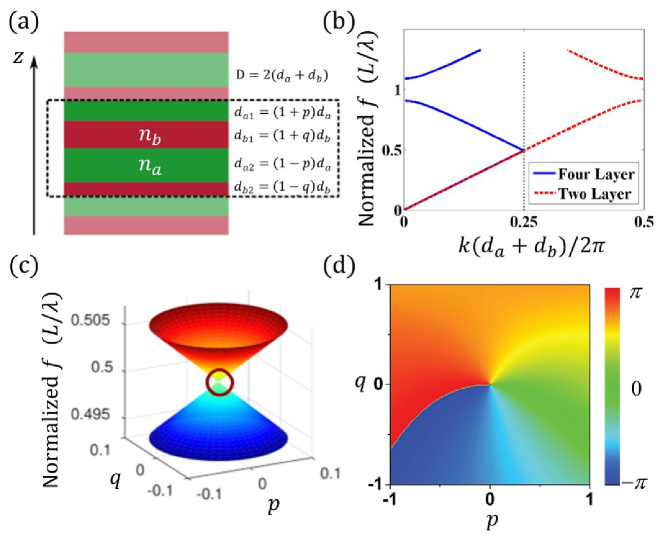
Figure 8: (a) A one-dimensional photonic crystal in Ref. wang17 with each unit cell including four layers where the thickness of each layer depends on parameters $p$ and $q$. (b) The band structure of the crystal with $p=q=0$. (c) Bandstructure in the ($p$, $q$) space with $k=\pi/2(d_{a}+d_{b})$. (d) The reflection phase for light incident upon such a photonic crystal from air, in the ($p$, $q$) space wang17 .

As an illustration, consider a one-dimensional photonic crystal in Ref. wang17 , the unit cell of which consists of four layers, with thickness $(1+p)d_{a}$, $(1+q)d_{b}$, $(1-p)d_{a}$, and $(1-q)d_{b}$. The band structure of such a crystal, in the special case where $p=q=0$, is shown in Fig. 8(b). In such a case, the four-layer unit cell is in fact not a primitive cell, and thus there is no band gap at the edge of the first Brilliouin zone $k=\pi/2(d_{a}+d_{b})$. At this $k$ point the bands are two-fold degenerate with linear dispersion along the $k$-axis. On the other hand, for $p$ and $q$ slightly deviating from 0, the four-layer unit cell becomes the primitive cell, and hence a band gap opens at the Brillouin zone edge, as shown in Fig. 8(c). The size of the gap scales linearly with respect to both $p$ and $q$. Therefore, one can show that in the three dimensional space of $k$, $p$ and $q$, the point $k=\pi/2(d_{a}+d_{b})$, $p=0$, and $q=0$ is in fact a Weyl point. The physical signature of such a Weyl point manifests in the reflection phase for a wave at a frequency of the Weyl point $f=0.49$ $L/\lambda$, incident from air onto the photonic crystal along the normal incidence direction. As one varies the parameters $p$ and $q$, the reflection phase winds around $p=q=0$. Remarkably, in this construction one can explore aspects of three-dimension Weyl-point physics using a simple one-dimensional structure.

IV.3 Adiabatic evolution in the parameter space

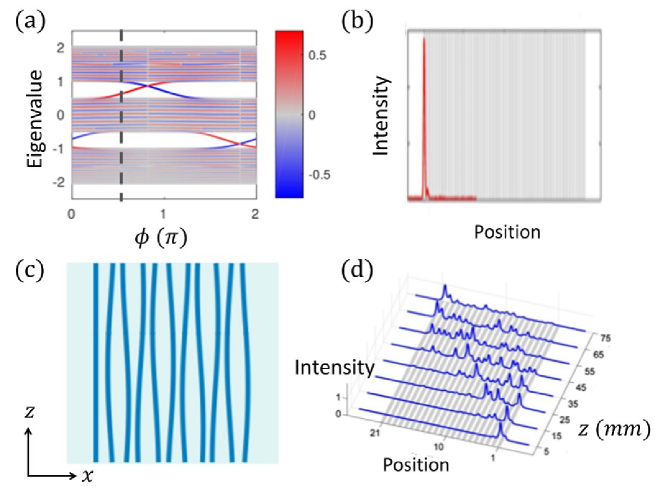
Figure 9: (a) Bandstructure of the Aubry-André model described by Eq. (30) composed of 99 sites with $g=1$, $V=0.5$, and $b=(\sqrt{5}+1)/2$. (b) Intensity distributions in the experiment show the edge state in the gap. Here $\phi=0.5\pi$. (c) Waveguide array where spacings between waveguides are slowly modified along the $z$-direction, as described by Eq. (31). (d) Intensity distributions versus the propagation distance $z$. Light is injected into the rightmost waveguide into a structure similar to (c). $\phi$ is changed from $0.35\pi$ to $1.75\pi$ adiabatically kraus12quasi .

In the previous section, for a system as described by a parametric Hamiltonian, the higher-dimensional physics is revealed by considering the properties of a set of physical structures with varying parameters. On the other hand, with a single physical structure, one can also explore higher dimensional physics by allowing the parameters to vary as a function of time, and considering the dynamics of such time-dependent parametric system.

As an illustration we consider consider the Aubry-André model aubry80 which describes a one-dimensional lattice

$$H=\sum_{m}g\left(a^{\dagger}_{m}a_{m+1}+a^{\dagger}_{m}a_{m-1}\right)+\sum_{m}a^{\dagger}_{m}a_{m}V\cos(2\pi bm+\phi),$$ (30)

where $a_{m}(a^{\dagger}_{m})$ is the annihilation (creation) operator on the $m$-th site, and $g$ is the coupling strength. $V$ is the amplitude of the on-site potential. $b$ and $\phi$ are parameters controlling the modulation of the on-site potential with respect to the site locations kraus12quasi . We note that for an irrational $b$ there is no periodicity in Eq. (30). In fact, in that case Eq. (30) describes a quasi-crystal.

By considering $\phi$ as a synthetic dimension, the Aubry-André model describes a synthetic two-dimensional space. In fact, it is known that Aubry-André model is closely related to the Quantum Hall system as described by a two dimensional model of a square lattice under a uniform magnetic field in the Landau gauge, as described by the Hamiltonian of Eq. (25). The $b$ in Eq. (30) maps to the magnetic field per unit cell in the two-dimensional model, and $\phi$ maps to the wavevector $k_{y}$ along periodic direction with the choice of the Landau gauge. Thus, for a finite structure, the eigenspectrum of the Aubry-André model exhibits gaps [Fig. 9(a)]. For particular values of $\phi$, an edge state can appear inside the gap [Fig. 9(b)]. The variation of eigenfrequencies as a function of $\phi$ corresponds directly to the dispersion of the one-way edge state in the Quantum Hall system.

In the finite-size Aubry-André model, suppose at $t=0$ the system is at an edge state on one of ends, by varying $\phi$ adiabatically as a function of time, the mode will evolve according to the edge state dispersion, eventually becomes a bulk state, and then reemerges as an edge state localized on the opposite end. Thus, the adiabatic evolution of the state in the time-dependent one-dimensional system provides a direct probe of the properties of the corresponding two-dimensional system.

Ref. kraus12quasi provides a direct experimental demonstration of such adiabatic evolution of the edge state. For this purpose, Ref. kraus12quasi made two important modification of the Aubry-André model. First of all, the Aubry-André model is transformed to:

$$H=g\sum_{m}\left[1+V\cos(2\pi bm+\phi)\right]a^{\dagger}_{m}a_{m+1}+\left[1-V\cos(2\pi b(m-1)+\phi)\right]a^{\dagger}_{m}a_{m-1}.$$ (31)

where the site-dependent modulation now appears in the coupling constant between nearest neighbor sites. Secondly, instead of considering time evolution, Ref. kraus12quasi consider an array of waveguides, where the variation of the field amplitudes along the propagation direction $z$ then provides a simulation of the temporal dynamics. With these modifications, Ref. kraus12quasi constructed a structure as shown in Fig. 9(c), where $\phi$ varies from $0.35\pi$ to $1.75\pi$ as a function $z$. The adiabatic dynamics is shown in 9(d). The injected light into the edge state at one end of the waeguide array evolves into a bulk state as light propagates along the $z$-direction, and eventually appear as an edge state on the other side, which is precisely the adiabatic evolution of the state as expected for the Aubry-André model.

The use of adiabatic evolution provides a powerful approach to explore higher dimension physics. In the waveguide array platform, this approach has also been used to experimentally explore topological phase transition verbin13 , as well as four-dimensional quantum Hall effects zilberberg18 . The connection of the one-dimensional Aubry-André model, which can be quasiperodic with an irrational $b$, to a two dimensional model also in fact points to a general connection between quasi-crystal in lower dimensional space and crystal structure in higher dimensional space. This connection has been previously explored to develop a computational tool for photonic quasicrystal rodriguez08 .

V Summary and outlook

To summarize this article, we provide a brief review of the concept of synthetic dimension in photonics, an area that has been rapidly developing in the past few years, in close connection with the developments of the gauge field and topological concepts in photonics. The initial motivation for exploring the synthetic dimension has been to develop a versatile approach in photonics for demonstrating many important fundamental physics effects, including in particular many important topological physics effects. And indeed, as we have seen in this review, a remarkably rich set of physics effects have been theoretically proposed and/or experimentally demonstrated using the synthetic dimension approach. We also envision that the concept of synthetic dimension will prove to be significant for practical applications, leading to new possibilities for manipulating and controlling some of the fundamental properties of light.

- (1) J. Ward and O. Benson, “WGM microresonators: sensing, lasing and fundamentaloptics with microspheres,” Laser Photonics Rev. 5, 553–570 (2011).
- (2) S. Feng, T. Lei, H. Chen, H. Cai, X. Luo, and A. W. Poon, “Silicon photonics: From a microresonator perspective,” Laser Photonics Rev. 6, 145–177 (2012).
- (3) M. Kawachi, “Silica waveguides on silicon and their application to integrated-optic components,” Opt. Quant. Electron. 22, 391–416 (1990).
- (4) J. D. Joannopoulos, P. R. Villeneuve, and S. Fan, “Photonic crystals: putting a new twist on light,” Nature 386, 143–149 (1997).
- (5) C. M. Soukoulis and M. Wegener, “Past achievements and future challenges in the development of three-dimensional photonic metamaterials,” Nat. Photonics 5, 523-530 (2011).
- (6) Y. Liu and X. Zhang, “Metamaterials: a new frontier of science and technology,” Chem. Soc. Rev. 40, 2494–2507 (2011).
- (7) A. Regensburger, C. Bersch, B. Hinrichs, G. Onishchukov, A. Schreiber, C. Silberhorn, and U. Peschel, “Photon propagation in a discrete fiber network: An interplay of coherence and losses,” Phys. Rev. Lett. 107, 233902 (2011).
- (8) A. Regensburger, C. Bersch, M.-A. Miri, G. Onishchukov, D. N. Christodoulides, and U. Peschel, “Parity-time synthetic photonic lattices,” Nature 488, 167–171 (2012).
- (9) A. Schwartz and B. Fischer, “Laser mode hyper-combs,” Opt. Express 21, 6196–6204 (2013).
- (10) X.-W. Luo, X. Zhou, C.-F. Li, J.-S. Xu, G.-C. Guo, and Z.-W. Zhou, “Quantum simulation of 2D topological physics in a 1D array of optical cavities,” Nat. Commun. 6, 7704 (2015).
- (11) L. Yuan, Y. Shi, and S. Fan, “Photonic gauge potential in a system with a synthetic frequency dimension,” Opt. Lett. 41, 741–744 (2016).
- (12) T. Ozawa, H. M. Price, N. Goldman, O. Zilberberg, and I. Carusotto, “Synthetic dimensions in integrated photonics: From optical isolation to four-dimensional quantum Hall physics,” Phys. Rev. A 93, 043827 (2016).
- (13) O. Boada, A. Celi, J. I. Latorre, and M. Lewenstein, “Quantum simulation of an extra dimension,” Phys. Rev. Lett. 108, 133001 (2012).
- (14) Y. E. Kraus and O. Zilberberg, “Topological equivalence between the Fibonacci quasicrystal and the Harper model,” Phys. Rev. Lett. 109, 116404 (2012).
- (15) F. Mei, S.-L. Zhu, Z.-M. Zhang, C. H. Oh, and N. Goldman, “Simulating topological insulators with cold atoms in a one-dimensional optical lattice,” Phys. Rev. A 85, 013638 (2012).
- (16) A. Gómez-León and G. Platero, “Floquet-Bloch theory and topology in periodically driven lattices,” Phys. Rev. Lett. 110, 200403 (2013).
- (17) S. Ganeshan, K. Sun, and S. Das Sarma, “,Topological zero-energy modes in gapless commensurate Aubry-André-Harper models,” Phys. Rev. Lett. 110, 180403 (2013).
- (18) Z. Xu, L. Li, and S. Chen, “Fractional topological states of dipolar fermions in one-dimensional optical superlattices,” Phys. Rev. Lett. 110, 215301 (2013).
- (19) Y. E. Kraus, Z. Ringel, and O. Zilberberg, “Four-dimensional quantum Hall effect in a two-dimensional quasicrystal,” Phys. Rev. Lett. 111, 226401 (2013).
- (20) A. Celi, P. Massignan, J. Ruseckas, N. Goldman, I. B. Spielman, G. Juzeliūnas, and M. Lewenstein, “Synthetic gauge fields in synthetic dimensions,” Phys. Rev. Lett. 112, 043001 (2014).
- (21) F. Mei, J.-B. You, D.-W. Zhang, X. C. Yang, R. Fazio, S.-L. Zhu, and L. C. Kwek, “Topological insulator and particle pumping in a one-dimensional shaken optical lattice,” Phys. Rev. A 90, 063638 (2014).
- (22) O. Boada, A. Celi, J. Rodríguez-Laguna, J. I. Latorre, and M. Lewenstein, “Quantum simulation of non-trivial topology,” New J. Phys. 17, 045007 (2015).
- (23) H. M. Price, O. Zilberberg, T. Ozawa, I. Carusotto, and N. Goldman, “Four-dimensional quantum Hall effect with ultracold atoms,” Phys. Rev. Lett. 115, 195303 (2015).
- (24) M. Mancini, G. Pagano, G. Cappellini, L. Livi, M. Rider, J. Catani, C. Sias, P. Zoller, M. Inguscio, M. Dalmonte, and L. Fallani “Observation of chiral edge states with neutral fermions in synthetic Hall ribbons,” Science 349, 1510–1513 (2015).
- (25) B. K. Stuhl, H.-I. Lu, L. M. Aycock, D. Genkina, I. B. Spielman, “Visualizing edge states with an atomic Bose gas in the quantum Hall regime,” Science 349, 1514–1518 (2015).
- (26) S. Nakajima, T. Tomita, S. Taie, T. Ichinose, H. Ozawa, L. Wang, M. Troyer, and Y. Takahashi, “Topological Thouless pumping of ultracold fermions,” Nat. Phys. 12, 296–300 (2016).
- (27) M. Lohse, C. Schweizer, O. Zilberberg, M. Aidelsburger, and I. Bloch, “A Thouless quantum pump with ultracold bosonic atoms in an optical superlattice,” Nat. Phys. 12, 350–354 (2016).
- (28) T.-S. Zeng, W. Zhu, and D. N. Sheng, “Fractional charge pumping of interacting bosons in one-dimensional superlattice,” Phys. Rev. B 94, 235139 (2016).
- (29) D. Suszalski and J. Zakrzewski, “Different lattice geometries with a synthetic dimension,” Phys. Rev. A 94, 033602 (2016).
- (30) L. Taddia, E. Cornfeld, D. Rossini, L. Mazza, E. Sela, and R. Fazio, “Topological fractional pumping with alkaline-earth-like atoms in synthetic lattices,” Phys. Rev. Lett. 118, 230402 (2017).
- (31) H. M. Price, T. Ozawa, and N. Goldman, “Synthetic dimensions for cold atoms from shaking a harmonic trap,” Phys. Rev. A 95, 023607 (2017).
- (32) I. Martin, G. Refael, and B. Halperin, “Topological frequency conversion in strongly driven quantum systems,” Phys. Rev. X 7, 041008 (2017).
- (33) Y. Baum and G. Refael, “Setting boundaries with memory: generation of topological boundary states in Floquet-induced synthetic crystals,” Phys. Rev. Lett. 120, 106402 (2018).
- (34) Y. Peng and G. Refael, “Topological energy conversion through bulk/boundary of driven systems,” arXiv:1801.05811.
- (35) M. Lohse, C. Schweizer, H. M. Price, O. Zilberberg, and I. Bloch, “Exploring 4D quantum Hall physics with a 2D topological charge pump,” Nature 553, 55–58 (2018).
- (36) C. Shang, X. Chen, W. Luo, and F. Ye, “Quantum anomalous Hall-quantum spin Hall effect in optical superlattices,” Opt. Lett. 43, 275–278 (2018).
- (37) F. W. Strauch and C. J. Williams, “Theoretical analysis of perfect quantum state transfer with superconducting qubits,” Phys. Rev. B 78, 094516 (2008).
- (38) D. I. Tsomokos, S. Ashhab, and F. Nori, “Using superconducting qubit circuits to engineer exotic lattice systems,” Phys. Rev. A 82, 052311 (2010).
- (39) F. Mei, Z.-Y. Xue, D.-W. Zhang, L. Tian, C. Lee, and S.-L. Zhu, “Witnessing topological Weyl semimetal phase in a minimal circuit-QED lattice,” Quantum Sci. Technol. 1, 015006 (2016).
- (40) S.-C. Zhang and J. Hu, “A four-dimensional generalization of the quantum Hall effect,” Science 294, 823–828 (2001).
- (41) X.-L. Qi, T. L. Hughes, and S.-C. Zhang, “Topological field theory of time-reversal invariant insulators,” Phys. Rev. B 78, 195424 (2008).
- (42) A. Kitaev, “Periodic table for topological insulators and superconductors,” AIP Conference Proceedings 1134, 22 (2009).
- (43) B. Lian and S.-C. Zhang, “Five-dimensional generalization of the topological Weyl semimetal,” Phys. Rev. B 94, 041105 (2016).
- (44) B. Lian and S.-C. Zhang, “Weyl semimetal and topological phase transition in five dimensions,” Phys. Rev. B 95, 235106 (2017).
- (45) R. Roy and F. Harper, “Periodic table for Floquet topological insulators,” Phys. Rev. B 96, 155118 (2017).
- (46) L. Yuan and S. Fan, “Bloch oscillation and unidirectional translation of frequency in a dynamically modulated ring resonator,” Optica 3, 1014–1018 (2016).
- (47) Q. Lin, M. Xiao, L. Yuan, and S. Fan, “Photonic Weyl point in a two-dimensional resonator lattice with a synthetic frequency dimension,” Nat. Commun. 7, 13731 (2016).
- (48) Y. Zhang and Y. Zhu, “Generation of Weyl points in coupled optical microdisk-resonator arrays via external modulation,” Phys. Rev. A 96, 013811 (2017).
- (49) L. Yuan, M. Xiao, Q. Lin, and S. Fan, “Synthetic space with arbitrary dimensions in a few rings undergoing dynamic modulation,” Phys. Rev. B 97, 104105 (2018).
- (50) Q. Lin, X.-Q. Sun, M. Xiao, S.-C. Zhang, and S. Fan, “Constructing three-dimensional photonic topological insulator using two-dimensional ring resonator lattice with a synthetic frequency dimension,” arXiv:1802.02597 (2018).
- (51) L. Yuan, Q. Lin, M. Xiao, A. Dutt, and S. Fan, “Pulse shortening in an actively mode-locked laser with parity-time symmetry,” (under preparation).
- (52) C. Qin, F. Zhou, Y. Peng, D. Sounas, X. Zhu, B. Wang, J. Dong, X. Zhang, A. Alù, and P. Lu, “Spectrum control through discrete frequency diffraction in the presence of photonic gauge potentials,” Phys. Rev. Lett. 120, 133901 (2018).
- (53) L. D. Tzuang, M. Soltani, Y. H. D. Lee, and M. Lipson, “High RF carrier frequency modulation in silicon resonators by coupling adjacent free-spectral-range modes,” Opt. Lett. 39, 1799–1802 (2014).
- (54) C. Wang, M. J. Burek, Z. Lin, H. A. Atikian, V. Venkataraman, I.-C. Huang, P. Stark, and M. Lončar, “Integrated high quality factor lithium niobate microdisk resonators,” Opt. Express 22, 30924–30933 (2014).
- (55) M. Zhang, C. Wang, R. Cheng, A. Shams-Ansari, and M. Lončar, “Monolithic ultra-high-Q lithium niobate microring resonator,” Optica 4, 1536–1537 (2017).
- (56) U. Peschel, C. Bersch, and G. Onishchukov, “Discreteness in time,” Open Phys. 6, 619–627 (2008).
- (57) C. Bersch, G. Onishchukov, and U. Peschel, “Experimental observation of spectral Bloch oscillations,” Opt. Lett. 34, 2372–2374 (2009).
- (58) B. A. Bell, K. Wang, A. S. Solntsev, D. N. Neshev, A. A. Sukhorukov, and B. J. Eggleton, “Spectral photonic lattices with complex long-range coupling,” Optica 4, 1433–1436 (2017).
- (59) L. Yuan, D.-w. Wang, S. Fan, “Synthetic gauge potential and effective magnetic field in a Raman medium undergoing molecular modulation,” Phys. Rev. A 95, 033801 (2017).
- (60) X.-W. Luo, X. Zhou, J.-S. Xu, C.-F. Li, G.-C. Guo, C. Zhang, and Z.-W. Zhou, “Synthetic-lattice enabled all-optical devices based on orbital angular momentum of light,” Nat. Commun. 8, 16097 (2017).
- (61) B. Y. Sun, X. W. Luo, M. Gong, G. C. Guo, and Z. W. Zhou, “Weyl semimetal phases and implementation in degenerate optical cavities,” Phys. Rev. A 96, 013857 (2017).
- (62) X.-F. Zhou, X.-W. Luo, S. Wang, G.-C. Guo, X. Zhou, H. Pu, and Z.-W. Zhou, “Dynamically manipulating topological physics and edge modes in a single degenerate optical cavity,” Phys. Rev. Lett. 118, 083603 (2017).
- (63) X.-W. Luo, C. Zhang, G.-C. Guo, and Z.-W. Zhou, “Topological photonic orbital-angular-momentum switch,” Phys. Rev. A 97, 043841 (2018).
- (64) M. Wimmer, A. Regensburger, C. Bersch, M.-A. Miri, S. Batz, G. Onishchukov, D. N. Christodoulides, and U. Peschel, “Optical diametric drive acceleration through action-reaction symmetry breaking,” Nat. Phys. 9, 780–784 (2013).
- (65) A. Regensburger, M.-A. Miri, C. Bersch, J. Näger, G. Onishchukov, D. N. Christodoulides, and U. Peschel, “Observation of defect states in PT-symmetric optical lattices,” Phys. Rev. Lett. 110, 223902 (2013).
- (66) M. Wimmer, A. Regensburger, M.-A. Miri, C. Bersch, D. N. Christodoulides, and U. Peschel, “Observation of optical solitons in PT-symmetric lattices,” Nat. Commun. 6, 7782 (2015).
- (67) M. Wimmer, H. M. Price, I. Carusotto, and U. Peschel, “Experimental measurement of the Berry curvature from anomalous transport,” Nat. Phys. 13, 545–550 (2017).
- (68) I. D. Vatnik, A. Tikan, G. Onishchukov, D. V. Churkin, and A. A. Sukhorukov, “Anderson localization in synthetic photonic lattices,” Sci. Rep. 7, 4301 (2017).
- (69) M. Wimmer and U. Peschel, “Observation of time reversed light propagation by an exchange of eigenstates,” Sci. Rep. 8, 2125 (2018).
- (70) E. Lustig, S. Weimann, Y. Plotnik, Y. Lumer, M. A. Bandres, A. Szameit, and M. Segev, “Photonic Topological Insulator in Synthetic Dimensions,” arXiv:1807.01983.
- (71) S. E. Harris and O. P. McDuff, “Theory of FM Laser Oscillation,” IEEE J. Quantum Electron. 1, 245–262 (1965).
- (72) O. P. McDuff and S. E. Harris, “Nonlinear Theory of the Internally Loss-Modulated Laser,” IEEE J. Quantum Electron. 3, 101–111 (1967).
- (73) H. A. Haus, “A Theory of Forced Mode Locking,” IEEE J. Quantum Electron. 11, 323–330 (1975).
- (74) H. A. Haus, “Mode-Locking of Lasers,” IEEE J. Sel. Top. Quantum Electron. 6, 1173–1185 (2000).
- (75) K. Fang, Z. Yu, and S. Fan, “Photonic Aharonov-Bohm effect based on dynamic modulation,” Phys. Rev. Lett. 108, 153901 (2012).
- (76) K. Fang, Z. Yu, and S. Fan, “Realizing effective magnetic field for photons by controlling the phase of dynamic modulation,” Nat. Photonics 6, 782–787 (2012).
- (77) L. Yuan and S. Fan, “Three-dimensional dynamic localization of light from a time-dependent effective gauge field for photons,” Phys. Rev. Lett. 114, 243901 (2015).
- (78) J. M. Luttinger, “The effect of a magnetic field on electrons in a periodic potential,” Phys. Rev. 84, 814–817 (1951).
- (79) F. Bloch, “Über die Quantenmechanik der Elektronen in Kristallgittern,” Z. Phys. 52, 555–600 (1929).
- (80) G. Lenz, I. Talanina, and C. M. de Sterke, “Bloch Oscillations in an Array of Curved Optical Waveguides,” Phys. Rev. Lett. 83, 963–966 (1999).
- (81) H. Trompeter, W. Krolikowski, D. N. Neshev, A. S. Desyatnikov, A. A. Sukhorukov, Y. S. Kivshar, T. Pertsch, U. Peschel, and F. Lederer, “Bloch Oscillations and Zener Tunneling in Two-Dimensional Photonic Lattices,” Phys. Rev. Lett. 96, 053903 (2006).
- (82) S. Longhi, “Optical Zener-Bloch oscillations in binary waveguide arrays,” Europhys. Lett. 76, 416–421 (2006).
- (83) F. Dreisow, A. Szameit, M. Heinrich, T. Pertsch, S. Nolte, A. Tünnermann, and S. Longhi, “Bloch-Zener Oscillations in Binary Superlattices,” Phys. Rev. Lett. 102, 076802 (2009).
- (84) M. Levy and P. Kumar, “Nonreciprocal Bloch oscillations in magneto-optic waveguide arrays,” Opt. Lett. 35, 3147–3149 (2010).
- (85) A. Kavokin, G. Malpuech, A. Di Carlo, and P. Lugli, “Photonic Bloch oscillations in laterally confined Bragg mirrors,” Phys. Rev. B 61, 4413–4416 (2000).
- (86) G. Malpuech, A. Kavokin, G. Panzarini, and A. Di Carlo, “Theory of photon Bloch oscillations in photonic crystals,” Phys. Rev. B 63, 035108 (2001).
- (87) R. Sapienza, P. Costantino, D. Wiersma, M. Ghulinyan, C. J. Oton, and L. Pavesi, “Optical Analogue of Electronic Bloch Oscillations,” Phys. Rev. Lett. 91, 263902 (2003).
- (88) V. Agarwal, J. A. del Río, G. Malpuech, M. Zamfirescu, A. Kavokin, D. Coquillat, D. Scalbert, M. Vladimirova, and B. Gil, “Photon Bloch Oscillations in Porous Silicon Optical Superlattices,” Phys. Rev. Lett. 92, 097401 (2004).
- (89) V. Lousse, and S. Fan, “Tunable terahertz Bloch oscillations in chirped photonic crystals,” Phys. Rev. B 72, 075119 (2005)
- (90) J. O. Estevez, J. Arriaga, E. Reyes-Ayona, and V. Agarwal, “Chirped dual periodic structures for photonic Bloch oscillations and Zener tunneling,” Opt. Express 23, 16500-16510 (2015).
- (91) S. Longhi, “Dynamic localization and Bloch oscillations in the spectrum of a frequency mode-locked laser,” Opt. Lett. 30, 786–788 (2005).
- (92) C. Bersch, G. Onishchukov, and U. Peschel, “Spectral and temporal Bloch oscillations in optical fibres,” Appl. Phys. B 104, 495–501 (2011).
- (93) H. Weyl, “Elektron und gravitation. I,” Z. Phys. 56, 330–352 (1929).
- (94) J. Bravo-Abad, L. Lu, L. Fu, H. Buljan, and M. Soljačić, “Weyl points in photonic-crystal superlattices,” 2D Mater. 2, 034013 (2015).
- (95) L. Lu, Z. Wang, D. Ye, L. Ran, L. Fu, J. D. Joannopoulos, M. Soljačić, “Experimental observation of Weyl points,” Science 349, 622–624 (2015).
- (96) W.-J. Chen, M. Xiao, and C. T. Chan, “Photonic crystals possessing multiple Weyl points and the experimental observation of robust surface states,” Nat. Commun. 7, 13038 (2015).
- (97) L. Wang, S.-K. Jian, and H. Yao, “Topological photonic crystal with equifrequency Weyl points,” Phys. Rev. A 93, 61801 (2016).
- (98) K. Sun, Z. Gu, H. Katsura, and S. Das Sarma, “Nearly flatbands with nontrivial topology,” Phys. Rev. Lett. 106, 236803 (2011).
- (99) E. Tang, J.-W. Mei, and X.-G. Wen, “High-temperature fractional quantum hall states,” Phys. Rev. Lett. 106, 236802 (2011).
- (100) R. O. Umucalılar and I. Carusotto, “Fractional quantum Hall states of photons in an array of dissipative coupled cavities,” 108, 206809 (2012).
- (101) D. F. Mross, J. Alicea, and O. I. Motrunich, “Explicit derivation of duality between a free dirac cone and quantum electrodynamics in (2+1) dimensions,” Phys. Rev. Lett. 117, 016802 (2016).
- (102) D. V. Strekalov, C. Marquardt, A. B. Matsko, H. G. L. Schwefel, and G. Leuchs, “Nonlinear and quantum optics with whispering gallery resonators,” J. Opt. 18, 123002 (2016).
- (103) T. Ozawa and I. Carusotto, “Synthetic Dimensions with Magnetic Fields and Local Interactions in Photonic Lattices,” Phys. Rev. Lett. 118, 013601 (2017).
- (104) M. V. Berry, “Quantal phase factors accompanying adiabatic changes,” Proc. R. Soc. London, Ser. A 392, 45–57 (1984)
- (105) R. Raffaele, “Manifestations of Berry’s phase in molecules and condensed matter,” J. Phys. Condens. Matter 12, R107–R143 (2000)
- (106) P. Roushan, C. Neill, Y. Chen, M. Kolodrubetz, C. Quintana, N. Leung, M. Fang, R. Barends, B. Campbell, Z. Chen, B. Chiaro, A. Dunsworth, E. Jeffrey, J. Kelly, A. Megrant, J. Mutus, P. J. J. O’Malley, D. Sank, A. Vainsencher, J. Wenner, T. White, A. Polkovnikov, A. N. Cleland, and J. M. Martinis, “Observation of topological transitions in interacting quantum circuits,” Nature 515, 241–244 (2014).
- (107) M. D. Schroer, M. H. Kolodrubetz, W. F. Kindel, M. Sandberg, J. Gao, M. R. Vissers, D. P. Pappas, A. Polkovnikov, and K. W. Lehnert, “Measuring a Topological Transition in an Artificial Spin-1/2 System,” Phys. Rev. Lett. 113, 050402 (2014).
- (108) C. G. Yale, F. J. Heremans, B. B. Zhou, A. Auer, G. Burkard, and D. D. Awschalom, “Optical manipulation of the Berry phase in a solid-state spin qubit,” Nat. Photonics 10, 184–189 (2016).
- (109) Q. Wang, M. Xiao, H. Liu, S. Zhu, and C. T. Chan, “Optical interface states protected by synthetic Weyl points,” Phys. Rev. X 7, 031032 (2017).
- (110) S. Aubry and G. André, “Analyticity breaking and anderson localization in incommensurate lattices,” Ann. Isr. Phys. Soc. 3, 133–164 (1980).
- (111) Y. E. Kraus, Y. Lahini, Z. Ringel, M. Verbin, and O. Zilberberg, “Topological states and adiabatic pumping in quasicrystals,” Phys. Rev. Lett. 109, 106402 (2012).
- (112) M. Verbin, O. Zilberberg, Y. E. Kraus, Y. Lahini, and Y. Silberberg, “Observation of topological phase transitions in photonic quasicrystals,” Phys. Rev. Lett. 110, 076403 (2013).
- (113) O. Zilberberg, S. Huang, J. Guglielmon, M. Wang, K. P. Chen, Y. E. Kraus, and M. C. Rechtsman, “Photonic topological boundary pumping as a probe of 4D quantum Hall physics,” Nature 553, 59–62 (2018).
- (114) A. W. Rodriguez, A. P. McCauley, Y. Avniel, and S. G. Johnson, “Computation and visualization of photonic quasicrystal spectra via Bloch’s theorem,” Phys. Rev. B 77, 104201 (2008).