Provably Positive High-Order Schemes for Ideal Magnetohydrodynamics: Analysis on General Meshes

Abstract

This paper proposes and analyzes arbitrarily high-order discontinuous Galerkin (DG) and finite volume methods which provably preserve the positivity of density and pressure for the ideal magnetohydrodynamics (MHD) on general meshes. Unified auxiliary theories are built for rigorously analyzing the positivity-preserving (PP) property of numerical MHD schemes with a Harten–Lax–van Leer (HLL) type flux on polytopal meshes in any space dimension. The main challenges overcome here include establishing certain relation between the PP property and a discrete divergence of magnetic field on general meshes, and estimating proper wave speeds in the HLL flux to ensure the PP property. In the 1D case, we prove that the standard DG and finite volume methods with the proposed HLL flux are PP, under a condition accessible by a PP limiter. For the multidimensional conservative MHD system, the standard DG methods with a PP limiter are not PP in general, due to the effect of unavoidable divergence error in the magnetic field. We construct provably PP high-order DG and finite volume schemes by proper discretization of the symmetrizable MHD system, with two divergence-controlling techniques: the locally divergence-free elements and an important penalty term. The former technique leads to zero divergence within each cell, while the latter controls the divergence error across cell interfaces. Our analysis reveals in theory that a coupling of these two techniques is very important for positivity preservation, as they exactly contribute the discrete divergence terms which are absent in standard multidimensional DG schemes but crucial for ensuring the PP property. Several numerical tests further confirm the PP property and the effectiveness of the proposed PP schemes. Unlike the conservative MHD system, the exact smooth solutions of the symmetrizable MHD system are proved to retain the positivity even if the divergence-free condition is not satisfied. Our analysis and findings further the understanding, at both discrete and continuous levels, of the relation between the PP property and the divergence-free constraint.

1 Introduction

This paper is concerned with highly accurate and robust numerical methods for the ideal compressible magnetohydrodynamics (MHD), which play an important role in many fields including astrophysics, plasma physics and space physics. When viscous, resistive and relativistic effects can be neglected, the governing equations of ideal MHD, which combine the equations of gas dynamics with the Maxwell equations, have been widely used to model the dynamics of electrically conducting fluids in the presence of magnetic field. The ideal MHD system can be written as

$${\bf U}_{t}+\nabla\cdot{\bf F}({\bf U})={\bf 0},$$ (1.1)

with an additional divergence-free constraint on the magnetic field

$$\nabla\cdot{\bf B}=0.$$ (1.2)

The conservative vector ${\bf U}=(\rho,\rho{\bf v},{\bf B},E)^{\top}$; in the $d$-dimensional case, the divergence operator $\nabla\cdot=\sum_{i=1}^{d}\frac{\partial}{\partial x_{i}}$, and the flux ${\bf F}=({\bf F}_{1},\dots,{\bf F}_{d})$ with

$${\bf F}_{i}({\bf U})=\Big{(}\rho v_{i},~{}\rho v_{i}{\bf v}-B_{i}{\bf B}+p_{\rm tot}{\bf e}_{i},~{}v_{i}{\bf B}-B_{i}{\bf v},~{}v_{i}(E+p_{\rm tot})-B_{i}({\bf v}\cdot{\bf B})\Big{)}^{\top}.$$

Here $\rho$ is the density, ${\bf v}=(v_{1},v_{2},v_{3})$ is the fluid velocity, ${\bf B}=(B_{1},B_{2},B_{3})$ denotes the magnetic field, $p_{\rm tot}=p+\frac{|{\bf B}|^{2}}{2}$ is the total pressure which consists of the gas pressure $p$ and the magnetic pressure, the row vector ${\bf e}_{i}$ denotes the $i$th row of the unit matrix of size 3, $E=\frac{1}{2}\left(\rho|{\bf v}|^{2}+|{\bf B}|^{2}\right)+\rho e$ is the total energy consisting of kinetic, magnetic and thermal energies, and $e$ denotes the specific internal energy. The system (1.1) is closed with an equation of state (EOS). Although the ideal EOS, $p=(\gamma-1)\rho e$, with a constant adiabatic index $\gamma$, is the most widely used choice, there are situations where it is more suitable to use other EOSs. A general EOS can be expressed as $p=p(\rho,e)$, which is assumed to satisfy (cf. [64]):

$$\mbox{if}\quad\rho>0,\quad\mbox{then}\quad e>0~{}\Leftrightarrow~{}p(\rho,e)>0.$$ (1.3)

This is a reasonable condition, and it holds for the ideal EOS with $\gamma>1$.

Although the satisfaction of the divergence-free condition (1.2) is not explicitly included in the system (1.1), the exact solution of (1.1) always preserves zero divergence in future time if the initial divergence is zero. However, due to truncation errors, most of the numerical MHD schemes for $d\geq 2$ lead to a nonzero numerical divergence in the magnetic field, even if the initial data satisfy (1.2). As it is widely known, large divergence error can lead to numerical instabilities or nonphysical features in the numerical solutions, cf. [11, 24, 8, 46, 34]. In the past several decades, many numerical techniques were proposed to control the divergence error or enforce the divergence-free condition in the discrete sense, including but not limited to: the projection method [11], the locally divergence-free methods [34, 60], the hyperbolic divergence cleaning method [20], the constrained transport method [24] and its variants (e.g., [43, 8, 3, 27, 45, 1, 35, 17, 25]), and the eight-wave methods (e.g., [40, 41, 12, 38]). The eight-wave method was first proposed by Powell [40, 41], based on appropriate discretization of the modified MHD equations of Godunov [28]:

$${\bf U}_{t}+\nabla\cdot{\bf F}({\bf U})=-(\nabla\cdot{\bf B})~{}{\bf S}({\bf U}),$$ (1.4)

where ${\bf S}({\bf U})=(0,~{}{\bf B},~{}{\bf v},~{}{\bf v}\cdot{\bf B})^{\top}.$ In some literature, (1.4) is also called Powell’s MHD system. The right-hand side term of (1.4), termed as the Godunov–Powell source term in the following, is proportional to $\nabla\cdot{\bf B}$. This means, at the continuous level, the Godunov form (1.4) and conservative form (1.1) are equivalent under the condition (1.2). However, the Godunov–Powell source term modifies the character of the MHD equations, making the system (1.4) Galilean invariant (cf. [21]), symmetrizable [28] and useful for designing entropy stable schemes (see, e.g., [12, 38]). These good properties do not hold anymore if the source term is dropped. As first demonstrated by Powell [41], the inclusion of the source term also helps advect the divergence away with the flow. This renders the eight-wave method a stable approach to control the divergence error, although some drawbacks [46] can be caused due to the loss of conservativeness.

In physics, the density, pressure and internal energy are positive. An equivalent mathematical description is that, the conservative vector ${\bf U}$ should stay in the set of physically admissible states defined by

$${\mathcal{G}}=\left\{{\bf U}=(\rho,{\bf m},{\bf B},E)^{\top}:\rho>0,~{}{\mathcal{E}}({\bf U}):=E-\frac{1}{2}\left(\frac{|{\bf m}|^{2}}{\rho}+|{\bf B}|^{2}\right)>0\right\},$$ (1.5)

where the condition (1.3) has been used, and ${\mathcal{E}}({\bf U})=\rho e$ denotes the internal energy. We are interested in positivity-preserving (PP) numerical schemes whose solutions always stay in ${\mathcal{G}}$. The motivation comes from that, once the negative density or negative pressure (internal energy) appears in the numerical solution, the corresponding discrete problem becomes ill-posed because of the loss of hyperbolicity, often causing the breakdown of the simulation codes. However, most the existing schemes for the ideal MHD are not PP in general, and may have a large risk of failure in solving MHD problems with low internal energy, low density, small plasma-beta and/or strong discontinuity. A few efforts were made to reduce this risk. Balsara and Spicer [7] tried to maintain positive pressure by switching the Riemann solvers for different wave situations. Janhunen [32] noticed the challenge of designing PP schemes for the conservative system (1.1), so he proposed a modified MHD system, which is similar to the Godunov form (1.4) but includes only the source term in the induction equation. By the discretization of his modified system, Janhunen [32] developed a 1D HLL-type Riemann solver, and numerically demonstrated its PP property which has not been proven yet. Bouchut, Klingenberg, and Waagan [9] skillfully derived several approximate multiwave Riemann solvers for the 1D ideal MHD, and gave the sufficient conditions for the solvers to satisfy the PP property and discrete entropy inequalities. Those conditions are met by explicit wave speeds estimated in [10], where the solvers were also implemented and multidimensional extension was discussed based on Janhunen’s modified system. Waagan [48] noticed the importance of proper discretization on Janhunen’s modified system, and designed a positive second-order MUSCL-Hancock scheme by the approximate Riemann solvers of [9, 10] and a new linear reconstruction. The robustness of that scheme was further demonstrated in [49] by extensive numerical tests and comparisons. In the last few years, significant advances have been made in developing bound-preserving high-order schemes for hyperbolic systems; see the pioneer works by Zhang and Shu [62, 63, 65], and more recent works, e.g., [31, 57, 37, 15, 53, 50, 59, 61]. Balsara [5] proposed a self-adjusting PP limiter to enforce the positivity of the reconstructed solutions in a finite volume method for (1.1). Cheng et al. [13] extended the PP limiter of [63, 64] to enforce the positivity of DG solutions for (1.1). These PP limiters [5, 13] are based on a presumed proposition that the cell-averaged solutions computed by those schemes always belong to $\mathcal{G}$. Such a proposition has not yet been rigorously proven for the methods in [5, 13], although it could be deduced for the 1D schemes in [13] under some assumptions. Using the presumed PP property of the Lax–Friedrichs (LF) scheme, Christlieb et al. [16, 14] developed PP high-order accurate finite difference schemes for (1.1) by extending the parametrized flux limiters [57, 56, 44]. It was numerically demonstrated that all the PP techniques mentioned above could enhance the robustness of some MHD codes, but few theoretical evidences were provided, especially in the multidimensional cases, to completely prove the PP property of full discretized schemes. In fact, finite numerical tests could be insufficient to genuinely demonstrate that a scheme is always PP under all circumstances. Therefore, it is highly significant to develop provably PP schemes and rigorous PP analysis techniques for the ideal MHD.

Seeking provably PP schemes for the ideal MHD is quite difficult, largely due to the intrinsic complexity of the MHD equations as well as the lack of sufficient knowledge about the underlying relation between the PP property and the divergence-free condition (1.2). It can seen from (1.5) that the difficulties mainly lie in maintaining the positivity of internal energy, whose calculation nonlinearly involves all the conservative variables. In most of the numerical MHD methods, the conservative quantities are themselves evolved according to their own conservation laws, which are seemingly unrelated to and numerically do not necessarily guarantee the positivity of the computed internal energy. In theory, it is indeed a challenge to make an a priori judgment on whether a scheme is always PP under all circumstances or not.

Recently, two progresses [51, 52] were made to rigorously analyze, understand and design provably PP methods for the ideal MHD. The first rigorous PP analysis was carried out in [51] for conservative finite volume and DG schemes for (1.1). The analysis revealed in theory that a discrete divergence-free (DDF) condition is crucial for designing the PP conservative schemes for (1.1). This finding is consistent with the relativistic MHD case [54]. It was also proved in [51] that if the proposed DDF condition is slightly violated, even the first-order multidimensional LF scheme for (1.1) is generally not PP, and using very small CFL number or many times larger numerical viscosity does not help to prevent this effect. The DDF condition relies on a combination of the information on adjacent cells, and thus is not ensured by a locally divergence-free approach. As a result, in the multidimensional cases, a usual PP limiter does not genuinely guarantee the PP property of the standard DG schemes for (1.1), even if the locally divergence-free DG element [34] is employed. Interestingly, on the other hand, at the PDE level the positivity preservation and the divergence-free constraint (1.1) are also inextricably linked for the ideal MHD equations. For the conservative system (1.1), Janhunen [32] noticed that the exact solutions to 1D Riemann problems can have negative pressure if the initial data has a jump in the normal component of the magnetic field (i.e., a nonzero divergence). Recently in [52], we first observed that the exact smooth solution of (1.1) may also fail to be PP if the divergence-free constraint (1.2) is (slightly) violated. Fortunately, in the present paper we find that the smooth solutions of the modified system (1.4) always retain the desired positivity even if the magnetic field is not divergence-free. All these findings motivate us to seek the multidimensional PP methods via proper discretization of the modified system (1.4) rather than the conservative system (1.1). Using the analysis techniques proposed in [51], we first successfully developed in [52] the multidimensional provably PP high-order DG methods for (1.4). Note that the study in [51, 52] was restricted to the schemes with the global LF flux on uniform Cartesian meshes. It is desirable to construct provably PP high-order schemes with lower dissipative numerical fluxes and on more general/unstructured meshes.

The aim of this paper is to present the rigorous analysis and a general framework for constructing provably PP high-order DG and finite volume methods with the HLL-type flux for the ideal MHD on general meshes. The contributions and significant innovations of this work are outlined as follows:

1. We present unified auxiliary theories for PP analysis of schemes with the HLL-type flux on general meshes for the ideal MHD in any space dimension. These provide a novel way to analytically extract the underlying relation between the PP property and the discrete divergence of magnetic field on an arbitrary polytopal mesh. Explicit estimates of the wave speeds in the HLL flux are technically derived to guarantee the provably PP property.

2. For the 1D MHD system (1.1), we prove the PP property of the standard finite volume and DG methods with the proposed HLL flux, under a condition accessible by a simple PP limiter.

3. In the multidimensional cases, we construct provably PP high-order DG methods based on the proposed HLL flux, a PP limiter [13], and a proper discretization of the modified MHD system (1.4) with two divergence-controlling techniques: the locally divergence-free elements and a novel discretization of the Godunov–Powell source term in an upwind manner according to the associated local wave speeds in the HLL flux. The former technique leads to zero divergence within each cell, while the latter controls the divergence error across cell interfaces. Our analysis clearly reveals in theory that a coupling of these two techniques is very important for positivity preservation, as they exactly contribute the discrete divergence terms which are absent in standard multidimensional DG schemes but crucial for ensuring the PP property. We also generalize the DDF condition of [51] to general meshes and derive sufficient conditions for achieving PP conservative schemes in the multiple dimensions.

4. We prove that the strong solution to the initial-value problem of the modified MHD system (1.4) preserves the positivity of density and pressure even if the divergence-free condition (1.2) is not satisfied. This feature, not enjoyed by the conservative system (1.1) (see [52]), can serve as a justification for designing provably PP multidimensional schemes based on the modified system (1.4).

The efforts mentioned above are novel and highly nontrivial. A key difficulty is to analytically quantify the relation of the PP property to the discrete divergence on general meshes. Especially, in the analysis of the positivity of ${\mathcal{E}}({\bf U})$, the discrete equations for the conservative variables are nonlinearly coupled, and the limiting values of the numerical solution at the interfaces of each cell are intrinsically connected by the discrete divergence. These make the PP analysis in the MHD case very complicated especially in the multidimensional cases, and some standard analysis techniques (cf. [63]) are inapplicable as demonstrated in [51]. We will skillfully address these challenges by a novel equivalent form of the set $\mathcal{G}$ and highly technical estimates. Note that a LF flux can be considered as a special HLL flux. Therefore, all the analyses in the this paper directly apply to the local and global LF fluxes. It is also worth mentioning that many multi-state or multi-wave HLL-type fluxes were developed or applied to the ideal MHD in the literature (e.g., [32, 30, 36, 39, 9, 4, 26, 6]), but only a few of them (cf. [30, 39, 9]) were shown to be PP for some 1D schemes. Moreover, their PP property for higher order schemes, in the multidimensional cases, and its relation to the divergence-free condition in the discrete sense have not yet been rigorously proved.

The paper is organized as follows. After establishing the auxiliary theories for our PP analysis on general meshes in Section 2, we present the 1D and multidimensional provably PP methods in Sections 3 and 4, respectively. We conduct numerical tests in Section 5 to verify the PP property and the effectiveness of the proposed PP techniques, before concluding the paper in Section 6. The positivity of strong solutions of the modified MHD system (1.4) is shown in Appendix A.

2 Auxiliary theories

In this section, we present the auxiliary results for our PP analysis on general meshes.

2.1 Properties of admissible state set

The function ${\mathcal{E}}({\bf U})$ in (1.5) is nonlinear with respect to $\bf U$, complicating the analysis of the PP property of a given scheme. The following equivalent form of ${\mathcal{G}}$ was proposed in [51].

Lemma 2.1.

The admissible state set ${\mathcal{G}}$ is equivalent to

$${\mathcal{G}}_{*}=\left\{{\bf U}=(\rho,{\bf m},{\bf B},E)^{\top}:\rho>0,~{}{\bf U}\cdot{\bf n}^{*}+\frac{|{\bf B}^{*}|^{2}}{2}>0,~{}\forall{\bf v}^{*},{\bf B}^{*}\in{\mathbb{R}}^{3}\right\},$$ (2.1)

where

$${\bf n}^{*}=\bigg{(}\frac{|{\bf v}^{*}|^{2}}{2},~{}-{\bf v}^{*},~{}-{\bf B}^{*},~{}1\bigg{)}^{\top}.$$

The proof of Lemma 2.1 can be found in [51]. As we can see, the equivalent set ${\mathcal{G}}_{*}$ is defined with two constraints linear with respect to $\bf U$, which give it advantages over the natural definition (1.5) in showing the PP property of numerical schemes. This novel equivalent form is a cornerstone of our PP analysis.

The convexity of admissible state set is desired and useful in bound-preserving analysis, as it helps simplify the analysis if the scheme can be reformulated into certain convex combinations; see e.g., [63, 65, 55, 50]. We have the convexity of ${\mathcal{G}}_{*}$, cf. [51].

Lemma 2.2.

The set ${\mathcal{G}}_{*}$ is convex. Moreover, $\lambda{\bf U}_{1}+(1-\lambda){\bf U}_{0}\in{\mathcal{G}}_{*}$ for any ${\bf U}_{1}\in{\mathcal{G}}_{*},{\bf U}_{0}\in\overline{\mathcal{G}}_{*}$ and $\lambda\in(0,1]$, where $\overline{\mathcal{G}}_{*}$ is the closure of ${\mathcal{G}}_{*}$.

2.2 Technical estimates relative to flux

2.2.1 Main estimates

We summarize our main estimate result in this subsection with the proof of it given later.

For the sake of convenience, we introduce the following notations, which will be frequently used in this paper. For any vector ${\bm{\xi}}=(\xi_{1},\cdots,\xi_{d})\in{\mathbb{R}}^{d}$, we define the inner products

$$\langle{\bm{\xi}},{\bf v}\rangle:=\sum_{k=1}^{d}{\xi}_{k}v_{k},\qquad\langle{\bm{\xi}},{\bf B}\rangle:=\sum_{k=1}^{d}{\xi}_{k}B_{k},\qquad\langle{\bm{\xi}},{\bf F}\rangle:=\sum_{k=1}^{d}{\xi}_{k}{\bf F}_{k}.$$

For any unit vector ${\bm{\xi}}\in{\mathbb{R}}^{d}$, define

$${\mathscr{C}}({\bf U};{\bm{\xi}}):=\frac{1}{\sqrt{2}}\left[{\mathscr{C}}_{s}^{2}+\frac{|{\bf B}|^{2}}{\rho}+\sqrt{\left({\mathscr{C}}_{s}^{2}+\frac{|{\bf B}|^{2}}{\rho}\right)^{2}-4\frac{{\mathscr{C}}_{s}^{2}\langle{\bm{\xi}},{\bf B}\rangle^{2}}{\rho}}\right]^{\frac{1}{2}},$$

where ${\mathscr{C}}_{s}:=\frac{p}{\rho\sqrt{2e}}$. Note that, for the ideal EOS, ${\mathscr{C}}_{s}=\sqrt{\frac{(\gamma-1)p}{2\rho}}$.

Recall that a technical inequality constructed in [51, Lemma 2.6] has played a pivotal role in the PP analysis on Cartesian meshes in [51, 52]. That inequality involves two states, which correspond to the numerical solutions at a couple of symmetric quadrature points on cell interfaces. The cells of a general mesh are generally non-symmetric, so that the results in [51] are inapplicable to the present analysis. To carry out PP analysis on a general mesh, we need to construct a (general) “multi-state” inequality, which is derived in the following theorem.

Theorem 2.1.

For $1\leq j\leq N$, let $s_{j}>0$ and the unit vector ${\bm{\xi}}^{(j)}\in{\mathbb{R}}^{d}$ satisfy

$$\sum_{j=1}^{N}s_{j}{\bm{\xi}}^{(j)}={\bf 0}.$$ (2.2)

Given $N$ admissible states ${\bf U}^{(j)}$, $1\leq j\leq N$, we define

$$\begin{split}\widehat{\alpha}_{j}&:=\max\left\{\big{\langle}{\bm{\xi}}^{(j)},{\bf v}^{(j)}\big{\rangle},\frac{1}{\sum\limits_{i=1}^{N}s_{i}}\sum_{i=1}^{N}s_{i}\left\langle{\bm{\xi}}^{(j)}-{\bm{\xi}}^{(i)},\frac{\sqrt{\rho^{(j)}}{\bf v}^{(j)}+\sqrt{\rho^{(i)}}{\bf v}^{(i)}}{\sqrt{\rho^{(j)}}+\sqrt{\rho^{(i)}}}\right\rangle\right\}\\ &\qquad+{\mathscr{C}}({\bf U}^{(j)};{{\bm{\xi}}^{(j)}})+\frac{2}{\sum\limits_{i=1}^{N}s_{i}}\sum_{i=1}^{N}s_{i}\frac{|{\bf B}^{(j)}-{\bf B}^{(i)}|}{\sqrt{\rho^{(j)}}+\sqrt{\rho^{(i)}}}.\end{split}$$ (2.3)

Then for any $\alpha_{j}\geq\widehat{\alpha}_{j}$, the state

$$\overline{\bf U}:=\frac{1}{{\sum\limits_{j=1}^{N}{s_{j}\alpha_{j}}}}\sum\limits_{j=1}^{N}{{{s_{j}\bigg{(}\alpha_{j}{{\bf U}^{(j)}-\Big{\langle}{\bm{\xi}}^{(j)},{\bf F}({\bf U}^{(j)})\Big{\rangle}}\bigg{)}}}},$$ (2.4)

belongs to ${\mathcal{G}}_{\rho}:=\{{\bf U}=(\rho,{\bf m},{\bf B},E)^{\top}:\rho>0\}$, and satisfies

$$\overline{\bf U}\cdot{\bf n}^{*}+\frac{|{\bf B}^{*}|^{2}}{2}\geq-\frac{{\bf v}^{*}\cdot{\bf B}^{*}}{{\sum\limits_{j=1}^{N}{s_{j}\alpha_{j}}}}\sum_{j=1}^{N}s_{j}\big{\langle}{\bm{\xi}}^{(j)},{\bf B}^{(j)}\big{\rangle},\quad\forall{\bf v}^{*},{\bf B}^{*}\in{\mathbb{R}}^{3}.$$ (2.5)

Furthermore, $\overline{\bf U}\in\overline{\mathcal{G}}_{*}$ if

$$\sum_{j=1}^{N}s_{j}\big{\langle}{\bm{\xi}}^{(j)},{\bf B}^{(j)}\big{\rangle}=0.$$ (2.6)

The proof of Theorem 2.1 and the construction of the inequality (2.5) are highly nontrivial and technical. For better legibility, we put the proof in Section 2.2.2. Here, we would like to briefly explain the result in Theorem 2.1, whose meaning will become more clear in the PP analysis in Sections 3 and 4. Let us consider a cell of the computational mesh, and assume it is a non-self-intersecting $d$-polytope with $N$ edges ($d=2$) or faces ($d=3$). The index $j$ on the variables in Theorem 2.1 represents the $j$th edge or face of the polytope, and $s_{j}$ and ${\bm{\xi}}^{(j)}$ respectively correspond to the $(d-1)$-dimensional Hausdorff measure and the unit outward normal vector of the $j$th edge or face. One can verify that the condition (2.2) holds naturally. In addition, ${\bf U}^{(j)}$ stands for the approximate values of ${\bf U}$ on the $j$th edge or face. The condition (2.6) is actually a DDF condition over the polytope.

Remark 2.1.

In Theorem 2.1, $\sum_{j=1}^{N}s_{j}\alpha_{j}$ is always positive, because

$$\sum\limits_{j=1}^{N}s_{j}\widehat{\alpha}_{j}>\frac{1}{\sum\limits_{i=1}^{N}s_{i}}\sum\limits_{j=1}^{N}s_{j}\sum_{i=1}^{N}s_{i}\left\langle{\bm{\xi}}^{(j)}-{\bm{\xi}}^{(i)},\frac{\sqrt{\rho^{(j)}}{\bf v}^{(j)}+\sqrt{\rho^{(i)}}{\bf v}^{(i)}}{\sqrt{\rho^{(j)}}+\sqrt{\rho^{(i)}}}\right\rangle=0.$$

Remark 2.2.

Theorem 2.1, particularly the inequality (2.5), clearly establishes a connection between the PP property and the discrete divergence of magnetic field, i.e., $\sum_{j=1}^{N}s_{j}\langle{\bm{\xi}}^{(j)},{\bf B}^{(j)}\rangle$. This will be a key point of our PP analysis. The right-hand side term of (2.5) is very important. The construction of this term is highly technical. If it is dropped, the inequality (2.5) would become invalid. As we will see, this term provides a way to take into account the discrete divergence in the PP analysis.

The following results are immediate corollaries of Theorem 2.1, which are useful for deriving PP numerical fluxes.

For any unit vector ${\bm{\xi}}\in{\mathbb{R}}^{d}$, and any pair of admissible states ${\bf U}$ and $\tilde{\bf U}$, we define

$$\alpha_{r}({\bf U},\tilde{\bf U};{\bm{\xi}}):=\max\left\{\langle{\bm{\xi}},{\bf v}\rangle,\frac{\sqrt{\rho}\langle{\bm{\xi}},{\bf v}\rangle+\sqrt{\tilde{\rho}}\langle{\bm{\xi}},\tilde{\bf v}\rangle}{\sqrt{\rho}+\sqrt{\tilde{\rho}}}\right\}+{\mathscr{C}}({\bf U};{\bm{\xi}})+\frac{|{\bf B}-\tilde{\bf B}|}{\sqrt{\rho}+\sqrt{\tilde{\rho}}},$$ (2.7)

$$\alpha_{l}({\bf U},\tilde{\bf U};{\bm{\xi}}):=\min\left\{\langle{\bm{\xi}},{\bf v}\rangle,\frac{\sqrt{\rho}\langle{\bm{\xi}},{\bf v}\rangle+\sqrt{\tilde{\rho}}\langle{\bm{\xi}},\tilde{\bf v}\rangle}{\sqrt{\rho}+\sqrt{\tilde{\rho}}}\right\}-{\mathscr{C}}({\bf U};{\bm{\xi}})-\frac{|{\bf B}-\tilde{\bf B}|}{\sqrt{\rho}+\sqrt{\tilde{\rho}}},$$ (2.8)

and

$$\alpha_{\star}({\bf U},\tilde{\bf U};{\bm{\xi}}):=\max\left\{|\langle{\bm{\xi}},{\bf v}\rangle|,\left|\frac{\sqrt{\rho}\langle{\bm{\xi}},{\bf v}\rangle+\sqrt{\tilde{\rho}}\langle{\bm{\xi}},\tilde{\bf v}\rangle}{\sqrt{\rho}+\sqrt{\tilde{\rho}}}\right|\right\}+{\mathscr{C}}({\bf U};{\bm{\xi}})+\frac{|{\bf B}-\tilde{\bf B}|}{\sqrt{\rho}+\sqrt{\tilde{\rho}}}.$$ (2.9)

Corollary 2.1.

For any ${\bf U},\tilde{\bf U}\in{\mathcal{G}}$, any unit vector ${\bm{\xi}}\in{\mathbb{R}}^{d}$, and

$$\forall\alpha\geq\alpha_{r}({\bf U},\tilde{\bf U};{\bm{\xi}}),\quad\forall\tilde{\alpha}\leq\alpha_{l}(\tilde{\bf U},{\bf U};{\bm{\xi}}),$$

the state

$$\overline{\bf U}:=\frac{1}{\alpha-\tilde{\alpha}}\Big{(}\alpha{\bf U}-\langle{\bm{\xi}},{\bf F}({\bf U})\rangle-\tilde{\alpha}\tilde{\bf U}+\langle{\bm{\xi}},{\bf F}(\tilde{\bf U})\rangle\Big{)},$$

belongs to ${\mathcal{G}}_{\rho}$ and satisfies

$$\overline{\bf U}\cdot{\bf n}^{*}+\frac{|{\bf B}^{*}|^{2}}{2}+\frac{{\bf v}^{*}\cdot{\bf B}^{*}}{\alpha-\tilde{\alpha}}\left(\langle{\bm{\xi}},{\bf B}\rangle-\langle{\bm{\xi}},\tilde{\bf B}\rangle\right)\geq 0,\quad\forall{\bf v}^{*},{\bf B}^{*}\in\mathbb{R}^{3}.$$ (2.10)

Furthermore, if $\langle{\bm{\xi}},{\bf B}\rangle-\langle{\bm{\xi}},\tilde{\bf B}\rangle=0,$ then $\overline{\bf U}\in\overline{\mathcal{G}}_{*}$.

Proof.

This directly follows from Theorem 2.1 with $N=2$, by taking

$$s_{1}=s_{2}=1,\ \,{\bm{\xi}}^{(1)}=-{\bm{\xi}}^{(2)}={\bm{\xi}},\ \,{\bf U}^{(1)}={\bf U},\ \ {\bf U}^{(2)}=\tilde{\bf U},\ \ \alpha_{1}=\alpha,\ \ \alpha_{2}=-\tilde{\alpha}. \blacksquare$$

Corollary 2.2.

Let ${\bf U},\tilde{\bf U}\in{\mathcal{G}}$, unit vector ${\bm{\xi}}\in{\mathbb{R}}^{d}$. For $\forall\alpha\geq\alpha_{\star}({\bf U},\tilde{\bf U};{\bm{\xi}})$, $\forall\tilde{\alpha}\geq\alpha_{\star}(\tilde{\bf U},{\bf U};{\bm{\xi}})$, the state

$$\overline{\bf U}:=\frac{1}{\alpha+\tilde{\alpha}}\Big{(}\alpha{\bf U}-\langle{\bm{\xi}},{\bf F}({\bf U})\rangle+\tilde{\alpha}\tilde{\bf U}+\langle{\bm{\xi}},{\bf F}(\tilde{\bf U})\rangle\Big{)},$$

belongs to ${\mathcal{G}}_{\rho}$ and satisfies

$$\overline{\bf U}\cdot{\bf n}^{*}+\frac{|{\bf B}^{*}|^{2}}{2}+\frac{{\bf v}^{*}\cdot{\bf B}^{*}}{\alpha+\tilde{\alpha}}\left(\langle{\bm{\xi}},{\bf B}\rangle-\langle{\bm{\xi}},\tilde{\bf B}\rangle\right)\geq 0,\quad\forall{\bf v}^{*},{\bf B}^{*}\in\mathbb{R}^{3}.$$ (2.11)

Furthermore, if $\langle{\bm{\xi}},{\bf B}\rangle-\langle{\bm{\xi}},\tilde{\bf B}\rangle=0,$ then $\overline{\bf U}\in\overline{\mathcal{G}}_{*}$.

Proof.

This is a direct consequence of Corollary 2.1. $\blacksquare$

Remark 2.3.

The inequalities (2.5), (2.10) and (2.11) extend the inequality constructed in [51, Lemma 2.6]. Corollaries 2.1 and 2.2 are useful for estimating the wave speeds to ensure the PP property of the HLL flux and local Lax-Friedrichs flux, respectively; see Theorem 2.2.

2.2.2 Proof of Theorem 2.1

We first establish several technical lemmas as the stepping stones on the path to prove Theorem 2.1.

For any ${\bf U}\in{\mathcal{G}}$ and ${\bf v}^{*},{\bf B}^{*}\in{\mathbb{R}}^{3}$, we define the nonzero vector $\bm{\theta}\in\mathbb{R}^{7}$ by

$${\bm{\theta}}({\bf U},{\bf v}^{*},{\bf B}^{*}):=\frac{1}{\sqrt{2}}\Big{(}{\bf B}-{\bf B}^{*},~{}\sqrt{\rho}({\bf v}-{\bf v}^{*}),~{}\sqrt{2\rho e}\Big{)}^{\top}.$$

As a novel point, introducing such a vector will bring much convenience in the following estimates and analyses. It is easy to verify that

$${\bf U}\cdot{\bf n}^{*}+\frac{|{\bf B}^{*}|^{2}}{2}=|{\bm{\theta}}|^{2}.$$ (2.12)

Lemma 2.3.

The set

$${\mathcal{G}}_{\rho}:=\big{\{}{\bf U}=(\rho,{\bf m},{\bf B},E)^{\top}:\rho>0\big{\}},$$

is a convex set. And for any ${\bf U}\in{\mathcal{G}}_{\rho}$, ${\bm{\xi}}\in\mathbb{R}^{d}$ and $\alpha>\langle{\bm{\xi}},{\bf v}\rangle$, it holds

$$\alpha{\bf U}-\langle{\bm{\xi}},{\bf F}({\bf U})\rangle\in{\mathcal{G}}_{\rho}.$$

Proof.

The result can be easily verified. $\blacksquare$

Lemma 2.4.

For any ${\bf U}\in{\mathcal{G}}$, any ${\bf v}^{*},{\bf B}^{*}\in{\mathbb{R}}^{3}$ and all $i\in\{1,2,3\}$, we have

$${\bf F}_{i}({\bf U})\cdot{\bf n}^{*}-B_{i}({\bf v}^{*}\cdot{\bf B}^{*})\leq v_{i}\sum_{k=4}^{7}\theta_{k}^{2}+v_{i}^{*}\bigg{(}\frac{1}{2}|{\bf B}|^{2}-{\bf B}\cdot{\bf B}^{*}\bigg{)}+{\mathscr{C}}_{i}|{\bm{\theta}}|^{2},$$ (2.13)

where ${\mathscr{C}}_{i}:={\mathscr{C}}({\bf U};{\bf e}_{i})$, and the vector ${\bf e}_{i}$ is the $i$-th row of the unit matrix of size 3.

Proof.

For any $i\in\{1,2,3\}$, we observe that

$${\bf F}_{i}({\bf U})\cdot{\bf n}^{*}-B_{i}({\bf v}^{*}\cdot{\bf B}^{*})=v_{i}\sum_{k=4}^{7}\theta_{k}^{2}+v_{i}^{*}\bigg{(}\frac{1}{2}|{\bf B}|^{2}-{\bf B}\cdot{\bf B}^{*}\bigg{)}+\Phi_{i},$$ (2.14)

where

$$\Phi_{i}({\bf U},{\bf v}^{*},{\bf B}^{*}):=p(v_{i}-v_{i}^{*})+\sum_{\begin{subarray}{c}1\leq k\leq 3\\ k\neq i\end{subarray}}\Big{(}B_{k}(v_{i}-v_{i}^{*})-B_{i}(v_{k}-v_{k}^{*})\Big{)}(B_{k}-B_{k}^{*}).$$

Let us show that $\Phi_{i}$ is bounded by ${\mathscr{C}}_{i}|{\bm{\theta}}|^{2}$ from above. We further observe that $\Phi_{i}$ is a quadratic form in the variables $\theta_{k}$, $1\leq k\leq 7$, and moreover, the coefficients of the quadratic form do not depend on ${\bf v}^{*}$ and ${\bf B}^{*}$. Specifically, for the fixed $i$, we have

$$p(v_{i}-v_{i}^{*})=2{\mathscr{C}}_{s}\frac{\sqrt{\rho}}{\sqrt{2}}(v_{i}-v_{i}^{*})\sqrt{\rho e}=2{\mathscr{C}}_{s}\theta_{3+i}\theta_{7},$$

$$\Big{(}B_{k}(v_{i}-v_{i}^{*})-B_{i}(v_{k}-v_{k}^{*})\Big{)}(B_{k}-B_{k}^{*})=2\frac{B_{k}}{\sqrt{\rho}}\theta_{3+i}\theta_{k}-2\frac{B_{i}}{\sqrt{\rho}}\theta_{3+k}\theta_{k},~{}~{}\forall k\neq i.$$

Define $i_{1}:=i~{}{\rm mod}~{}3+1$ and $i_{2}:=(i+1)~{}{\rm mod}~{}3+1$, and

$$\tilde{\bm{\theta}}:=\big{(}\theta_{3+i},~{}\theta_{3+i_{1}},~{}\theta_{3+i_{2}},~{}\theta_{i_{1}},~{}\theta_{i_{2}},~{}\theta_{7}\big{)}^{\top},$$

then

$$\Phi_{i}=2{\mathscr{C}}_{s}\theta_{3+i}\theta_{7}+2\sum_{k\in\{i_{1},i_{2}\}}\bigg{(}\frac{B_{k}}{\sqrt{\rho}}\theta_{3+i}\theta_{k}-\frac{B_{i}}{\sqrt{\rho}}\theta_{3+k}\theta_{k}\bigg{)}=\tilde{\bm{\theta}}^{\top}{\bf A}\tilde{\bm{\theta}},$$

where

$${\bf A}=\begin{pmatrix}0&0&0&B_{i_{1}}\rho^{-\frac{1}{2}}&B_{i_{2}}\rho^{-\frac{1}{2}}&{\mathscr{C}}_{s}\\ 0&0&0&-B_{i}\rho^{-\frac{1}{2}}&0&0\\ 0&0&0&0&-B_{i}\rho^{-\frac{1}{2}}&0\\ B_{i_{1}}\rho^{-\frac{1}{2}}&-B_{i}\rho^{-\frac{1}{2}}&0&0&0&0\\ B_{i_{2}}\rho^{-\frac{1}{2}}&0&-B_{i}\rho^{-\frac{1}{2}}&0&0&0\\ {\mathscr{C}}_{s}&0&0&0&0&0\end{pmatrix}.$$

The spectral radius of ${\bf A}$ is ${\mathscr{C}}_{i}$. Therefore,

$$|\Phi_{i}|\leq|\tilde{\bm{\theta}}^{\top}{\bf A}\tilde{\bm{\theta}}|\leq{\mathscr{C}}_{i}|\tilde{\bm{\theta}}|^{2}={\mathscr{C}}_{i}(|{\bm{\theta}}|^{2}-\theta_{i}^{2})\leq{\mathscr{C}}_{i}|{\bm{\theta}}|^{2},$$

which along with the identity (2.14) imply (2.13). $\blacksquare$

For any unit vector ${\bm{\xi}}\in{\mathbb{R}}^{d}$, we introduce a matrix ${\bf T}_{\bm{\xi}}:={\rm diag}\big{\{}1,\widehat{\bf T}_{{\bm{\xi}}},\widehat{\bf T}_{{\bm{\xi}}},1\big{\}}$, with the rotational matrix $\widehat{\bf T}_{{\bm{\xi}}}$ defined as follows:
(i). In $d=1$, ${\bm{\xi}}=\xi$ is a scalar of value 1 or $-1$, and $\widehat{\bf T}_{{\bm{\xi}}}$ is defined as ${\rm diag}\{\xi,1,1\}$.
(ii). In $d=2$, let $(\cos\varphi,\sin\varphi)$ be the polar coordinate representation of ${\bm{\xi}}$, and

$$\widehat{\bf T}_{{\bm{\xi}}}:=\begin{pmatrix}\cos\varphi~{}&~{}\sin\varphi~{}&~{}0\\ -\sin\varphi~{}&~{}\cos\varphi~{}&~{}0\\ 0~{}&~{}0~{}&~{}1\end{pmatrix}.$$

(iii). In $d=3$, let $(\sin\phi\cos\varphi,\sin\phi\sin\varphi,\cos\phi)$ be the spherical coordinate representation of ${\bm{\xi}}$, and

$$\widehat{\bf T}_{{\bm{\xi}}}:=\begin{pmatrix}\sin\phi\cos\varphi~{}&~{}\sin\phi\sin\varphi~{}&~{}\cos\phi\\ -\sin\varphi~{}&~{}\cos\varphi~{}&~{}0\\ -\cos\phi\cos\varphi~{}&~{}-\cos\phi\sin\varphi~{}&~{}\sin\phi\end{pmatrix}.$$

The rotational invariance property of the $d$-dimensional MHD system (1.1) implies

$$\langle{\bm{\xi}},{\bf F}({\bf U})\rangle={\bf T}_{\bm{\xi}}^{-1}{\bf F}_{1}({\bf T}_{\bm{\xi}}{\bf U}).$$ (2.15)

This helps us extend Lemma 2.4 to the following general case.

Lemma 2.5.

For any ${\bf U}\in{\mathcal{G}}$, any ${\bf v}^{*},{\bf B}^{*}\in{\mathbb{R}}^{3}$ and any unit vector ${\bm{\xi}}\in\mathbb{R}^{d}$, it holds

$$\langle{\bm{\xi}},{\bf F}({\bf U})\rangle\cdot{\bf n}^{*}-\langle{\bm{\xi}},{\bf B}\rangle({\bf v}^{*}\cdot{\bf B}^{*})\leq\langle{\bm{\xi}},{\bf v}\rangle\sum_{k=4}^{7}\theta_{k}^{2}+\langle{\bm{\xi}},{\bf v}^{*}\rangle\Big{(}\frac{1}{2}|{\bf B}|^{2}-{\bf B}\cdot{\bf B}^{*}\Big{)}+{\mathscr{C}}({\bf U};{\bm{\xi}})|{\bm{\theta}}|^{2}.$$

Proof.

Let $\hat{\bf U}:={\bf T}_{\bm{\xi}}{\bf U}$, $\hat{\bf v}^{*}:=\widehat{\bf T}_{\bm{\xi}}{\bf v}^{*}$, $\hat{\bf B}:=\widehat{\bf T}_{\bm{\xi}}{\bf B}^{*}$, $\hat{\bm{\theta}}:={\bm{\theta}}(\hat{\bf U},\hat{\bf v}^{*},\hat{\bf B}^{*})$, and

$$\hat{\bf n}^{*}:=\bigg{(}\frac{|\hat{\bf v}^{*}|^{2}}{2},~{}-\hat{\bf v}^{*},~{}-\hat{\bf B}^{*},~{}1\bigg{)}^{\top}={\bf T}_{\bm{\xi}}{\bf n}^{*}.$$

By the definition (1.5), one can easily verify $\hat{\bf U}\in{\mathcal{G}}$, which, together with the orthogonality of ${\bf T}_{\bm{\xi}}^{-1}$ and $\widehat{\bf T}_{\bm{\xi}}^{-1}$, imply

$$\langle{\bm{\xi}},{\bf F}({\bf U})\rangle\cdot{\bf n}^{*}-\langle{\bm{\xi}},{\bf B}\rangle({\bf v}^{*}\cdot{\bf B}^{*})$$

$$\overset{\eqref{eq:MHD:rotINV}}{=}\big{(}{\bf T}_{\bm{\xi}}^{-1}{\bf F}_{1}(\hat{\bf U})\big{)}\cdot\big{(}{\bf T}_{\bm{\xi}}^{-1}\hat{\bf n}^{*}\big{)}-\hat{B}_{1}(\widehat{\bf T}_{\bm{\xi}}^{-1}\hat{\bf v}^{*})\cdot(\widehat{\bf T}_{\bm{\xi}}^{-1}\hat{\bf B}^{*})$$

$$={\bf F}_{1}(\hat{\bf U})\cdot\hat{\bf n}^{*}-\hat{B}_{1}(\hat{\bf v}^{*}\cdot\hat{\bf B}^{*})$$

$$\overset{\eqref{eq:wklieq1}}{\leq}\hat{v}_{1}\sum_{k=4}^{7}\hat{\theta}_{k}^{2}+\hat{v}_{1}^{*}\bigg{(}\frac{1}{2}|\hat{\bf B}|^{2}-\hat{\bf B}\cdot\hat{\bf B}^{*}\bigg{)}+{\mathscr{C}}_{1}(\hat{\bf U})|\hat{\bm{\theta}}|^{2}$$

$$=\langle{\bm{\xi}},{\bf v}\rangle\sum_{k=4}^{7}\theta_{k}^{2}+\langle{\bm{\xi}},{\bf v}^{*}\rangle\Big{(}\frac{1}{2}|{\bf B}|^{2}-{\bf B}\cdot{\bf B}^{*}\Big{)}+{\mathscr{C}}({\bf U};{\bm{\xi}})|{\bm{\theta}}|^{2}.$$

The proof is completed. $\blacksquare$

Lemma 2.6.

Assume that ${\bf U}=(\rho,\rho{\bf v},{\bf B},E)^{\top}\in{\mathcal{G}}$, $\tilde{\bf U}=(\tilde{\rho},\tilde{\rho}\tilde{\bf v},\tilde{\bf B},\tilde{E})^{\top}\in{\mathcal{G}}$. For $\forall{\bf v}^{*},{\bf B}^{*}\in{\mathbb{R}}^{3}$, $\forall{\bm{\xi}}\in\mathbb{R}^{d}$ and $\forall\delta\in\mathbb{R}$, it holds

$$\langle{\bm{\xi}},{\bf v}^{*}\rangle\left[\bigg{(}\frac{\big{|}{\bf B}\big{|}^{2}}{2}-{\bf B}\cdot{\bf B}^{*}\bigg{)}-\bigg{(}\frac{\big{|}\tilde{\bf B}\big{|}^{2}}{2}-\tilde{\bf B}\cdot{\bf B}^{*}\bigg{)}\right]$$ (2.16)

$$\qquad\leq\langle{\bm{\xi}},\delta{\bf v}+(1-\delta)\tilde{\bf v}\rangle\sum_{k=1}^{3}\big{(}\theta_{k}^{2}-\tilde{\theta}_{k}^{2}\big{)}+|{\bm{\xi}}|f({\bf U},\tilde{\bf U};\delta)\big{(}|{{\bm{\theta}}}|^{2}+|{\tilde{\bm{\theta}}}|^{2}\big{)},$$

where ${\bm{\theta}}:={\bm{\theta}}({\bf U},{\bf v}^{*},{\bf B}^{*})$ and ${\tilde{\bm{\theta}}}:={\bm{\theta}}({{\tilde{\bf U}}},{\bf v}^{*},{\bf B}^{*})$, and $f({\bf U},\tilde{\bf U};\delta)$ is defined by

$$f({\bf U},\tilde{\bf U};\delta):=\frac{|\tilde{\bf B}-{\bf B}|}{\sqrt{2}}\sqrt{\frac{\delta^{2}}{\rho}+\frac{(1-\delta)^{2}}{\tilde{\rho}}}.$$ (2.17)

Proof.

With the aid of the Cauchy-Schwarz inequality, we have

$$\langle{\bm{\xi}},{\bf v}^{*}\rangle\left[\bigg{(}\frac{\big{|}{\bf B}\big{|}^{2}}{2}-{\bf B}\cdot{\bf B}^{*}\bigg{)}-\bigg{(}\frac{\big{|}\tilde{\bf B}\big{|}^{2}}{2}-\tilde{\bf B}\cdot{\bf B}^{*}\bigg{)}\right]-\langle{\bm{\xi}},\delta{\bf v}+(1-\delta)\tilde{\bf v}\rangle\sum_{k=1}^{3}\big{(}\theta_{k}^{2}-\tilde{\theta}_{k}^{2}\big{)}$$

$$=\left(\frac{\delta}{2}\langle{\bm{\xi}},{\bf v}-{\bf v}^{*}\rangle+\frac{1-\delta}{2}\langle{\bm{\xi}},\tilde{\bf v}-{\bf v}^{*}\rangle\right)({\bf\tilde{B}}-{\bf B})\cdot\big{(}{\bf B}+\tilde{\bf B}-2{\bf B}^{*}\big{)}$$

$$\leq\frac{|{\bm{\xi}}|}{2}\left(\frac{|\delta|}{\sqrt{\rho}}\sqrt{\rho}|{\bf v}-{\bf v}^{*}|+\frac{|1-\delta|}{\sqrt{\tilde{\rho}}}\sqrt{\tilde{\rho}}|\tilde{\bf v}-{\bf v}^{*}|\right)|{\bf\tilde{B}}-{\bf B}|\big{(}|{\bf B}-{\bf B}^{*}|+|\tilde{\bf B}-{\bf B}^{*}|\big{)}$$

$$\leq\frac{|{\bm{\xi}}|}{2}\sqrt{\frac{\delta^{2}}{\rho}+\frac{(1-\delta)^{2}}{\tilde{\rho}}}\sqrt{\rho|{\bf v}-{\bf v}^{*}|^{2}+\tilde{\rho}|\tilde{\bf v}-{\bf v}^{*}|^{2}}|{\bf\tilde{B}}-{\bf B}|\sqrt{2(|{\bf B}-{\bf B}^{*}|^{2}+|\tilde{\bf B}-{\bf B}^{*}|^{2})}$$

$$=2|{\bm{\xi}}|f({\bf U},\tilde{\bf U};\delta)\sqrt{\sum_{k=4}^{6}\big{(}\theta_{k}^{2}+\tilde{\theta}_{k}^{2}\big{)}}\sqrt{\sum_{k=1}^{3}\big{(}\theta_{k}^{2}+\tilde{\theta}_{k}^{2}\big{)}}$$

$$\leq|{\bm{\xi}}|f({\bf U},\tilde{\bf U};\delta)\sum_{k=1}^{6}\big{(}\theta_{k}^{2}+\tilde{\theta}_{k}^{2}\big{)}\leq|{\bm{\xi}}|f({\bf U},\tilde{\bf U};\delta)\big{(}|{{\bm{\theta}}}|^{2}+|{\tilde{\bm{\theta}}}|^{2}\big{)}.$$

The proof is completed. $\blacksquare$

We are now ready to prove Theorem 2.1.

Proof.

Note that $\alpha_{j}\geq\widehat{\alpha}_{j}>\langle{\bm{\xi}}^{(j)},{\bf v}^{(j)}\rangle$. It follows from Lemma 2.3 that $\alpha_{j}{\bf U}^{(j)}-\langle{\bm{\xi}}^{(j)},{\bf F}({\bf U}^{(j)})\rangle\in{\mathcal{G}}_{\rho}$, and furthermore $\overline{\bf U}\in{\mathcal{G}}_{\rho}$, by noting that $\sum_{j=1}^{N}s_{j}\alpha_{j}>0$ (see Remark 2.1).

We then focus on proving the inequality (2.5), or equivalently,

$$\sum_{j=1}^{N}s_{j}\Pi^{(j)}\leq\sum_{j=1}^{N}\alpha_{j}|{\bm{\theta}}^{(j)}|^{2},$$ (2.18)

where ${\bm{\theta}}^{(j)}:={\bm{\theta}}({\bf U}^{(j)},{\bf v}^{*},{\bf B}^{*})$, and

$$\Pi^{(j)}:=\langle{\bm{\xi}}^{(j)},{\bf F}({\bf U}^{(j)})\rangle\cdot{\bf n}^{*}-\langle{\bm{\xi}}^{(j)},{\bf B}^{(j)}\rangle({\bf v}^{*}\cdot{\bf B}^{*}).$$

Using Lemma 2.5 gives

$$\sum_{j=1}^{N}s_{j}\Pi^{(j)} \leq\left\{\sum_{j=1}^{N}s_{j}\langle{\bm{\xi}}^{(j)},{\bf v}^{(j)}\rangle\sum_{k=4}^{7}\big{|}\theta_{k}^{(j)}\big{|}^{2}\right\}+\left\{\sum_{j=1}^{N}s_{j}{\mathscr{C}}({\bf U}^{(j)};{\bm{\xi}})|{\bm{\theta}}^{(j)}|^{2}\right\}$$

$$\quad+\left\{\sum_{j=1}^{N}s_{j}\langle{\bm{\xi}}^{(j)},{\bf v}^{*}\rangle\Big{(}\frac{1}{2}|{\bf B}^{(j)}|^{2}-{\bf B}^{(j)}\cdot{\bf B}^{*}\Big{)}\right\}$$

$$=:\Pi_{1}+\Pi_{2}+\Pi_{3}.$$ (2.19)

Noting that, for any $1\leq i\leq N$, the hypothesis (2.2) implies

$$\sum_{j=1}^{N}s_{j}\langle{\bm{\xi}}^{(j)},{\bf v}^{*}\rangle=\left\langle\sum_{j=1}^{N}s_{j}{\bm{\xi}}^{(j)},{\bf v}^{*}\right\rangle=0.$$

Thus we can reformulate $\Pi_{3}$ as

$$\Pi_{3} =\sum_{j=1}^{N}s_{j}\langle{\bm{\xi}}^{(j)},{\bf v}^{*}\rangle\Big{(}\frac{1}{2}|{\bf B}^{(j)}|^{2}-{\bf B}^{(j)}\cdot{\bf B}^{*}\Big{)}-\sum_{j=1}^{N}s_{j}\langle{\bm{\xi}}^{(j)},{\bf v}^{*}\rangle\Big{(}\frac{1}{2}|{\bf B}^{(i)}|^{2}-{\bf B}^{(i)}\cdot{\bf B}^{*}\Big{)}$$

$$=\sum_{j=1}^{N}s_{j}\langle{\bm{\xi}}^{(j)},{\bf v}^{*}\rangle\left[\Big{(}\frac{1}{2}|{\bf B}^{(j)}|^{2}-{\bf B}^{(j)}\cdot{\bf B}^{*}\Big{)}-\Big{(}\frac{1}{2}|{\bf B}^{(i)}|^{2}-{\bf B}^{(i)}\cdot{\bf B}^{*}\Big{)}\right]=:\sum_{j=1}^{N}s_{j}\Pi_{3}^{(ji)},$$

for any $1\leq i\leq N$. For any $\delta\in\mathbb{R}$, it follows from Lemma 2.6 that

$$\begin{split}\Pi_{3}^{(ji)}&\leq\langle{\bm{\xi}}^{(j)},\delta{\bf v}^{(j)}+(1-\delta){\bf v}^{(i)}\rangle\sum_{k=1}^{3}\left(|\theta_{k}^{(j)}|^{2}-|\theta_{k}^{(i)}|^{2}\right)\\ &\quad+f({\bf U}^{(j)},{\bf U}^{(i)};\delta)\big{(}|{\bm{\theta}}^{(j)}|^{2}+|{\bm{\theta}}^{(i)}|^{2}\big{)}.\end{split}$$ (2.20)

In particular, we take the free variable $\delta$ as ${\sqrt{\rho^{(j)}}}/\big{(}\sqrt{\rho^{(j)}}+\sqrt{\rho^{(i)}}\big{)}$, which gives the Roe-type weighted average. Let

$$\bar{\bf v}^{(ji)}:=\frac{\sqrt{\rho^{(j)}}{\bf v}^{(j)}+\sqrt{\rho^{(i)}}{\bf v}^{(i)}}{\sqrt{\rho^{(j)}}+\sqrt{\rho^{(i)}}},$$

then the inequality (2.20) becomes

$$\Pi_{3}^{(ji)}\leq\left\langle{\bm{\xi}}^{(j)},\bar{\bf v}^{(ji)}\right\rangle\sum_{k=1}^{3}\left(|\theta_{k}^{(j)}|^{2}-|\theta_{k}^{(i)}|^{2}\right)+\frac{|{\bf B}^{(j)}-{\bf B}^{(i)}|}{\sqrt{\rho^{(j)}}+\sqrt{\rho^{(i)}}}\big{(}|{\bm{\theta}}^{(j)}|^{2}+|{\bm{\theta}}^{(i)}|^{2}\big{)}.$$ (2.21)

It follows that

$$\left(\sum_{i=1}^{N}s_{i}\right)\Pi_{3} =\sum_{i=1}^{N}\sum_{j=1}^{N}s_{i}s_{j}\Pi_{3}^{(ji)}$$ (2.22)

$$\leq\sum_{i=1}^{N}\sum_{j=1}^{N}s_{i}s_{j}\left\langle{\bm{\xi}}^{(j)},\bar{\bf v}^{(ji)}\right\rangle\sum_{k=1}^{3}\left(|\theta_{k}^{(j)}|^{2}-|\theta_{k}^{(i)}|^{2}\right)$$

$$\quad+\sum_{i=1}^{N}\sum_{j=1}^{N}s_{i}s_{j}\frac{|{\bf B}^{(j)}-{\bf B}^{(i)}|}{\sqrt{\rho^{(j)}}+\sqrt{\rho^{(i)}}}\big{(}|{\bm{\theta}}^{(j)}|^{2}+|{\bm{\theta}}^{(i)}|^{2}\big{)}.$$

By $\bar{\bf v}^{(ji)}=\bar{\bf v}^{(ij)}$ and the technique of exchanging indexes $i$ and $j$, we obtain

$$\sum_{i=1}^{N}\sum_{j=1}^{N}s_{i}s_{j}\left\langle{\bm{\xi}}^{(j)},\bar{\bf v}^{(ji)}\right\rangle\sum_{k=1}^{3}|\theta_{k}^{(i)}|^{2}=\sum_{i=1}^{N}\sum_{j=1}^{N}s_{i}s_{j}\left\langle{\bm{\xi}}^{(i)},\bar{\bf v}^{(ji)}\right\rangle\sum_{k=1}^{3}|\theta_{k}^{(j)}|^{2},$$

$$\sum_{i=1}^{N}\sum_{j=1}^{N}s_{i}s_{j}\frac{|{\bf B}^{(j)}-{\bf B}^{(i)}|}{\sqrt{\rho^{(j)}}+\sqrt{\rho^{(i)}}}|{\bm{\theta}}^{(i)}|^{2}=\sum_{i=1}^{N}\sum_{j=1}^{N}s_{i}s_{j}\frac{|{\bf B}^{(j)}-{\bf B}^{(i)}|}{\sqrt{\rho^{(j)}}+\sqrt{\rho^{(i)}}}|{\bm{\theta}}^{(j)}|^{2}.$$

Therefore, the inequality (2.22) can be rewritten as

$$\left(\sum_{i=1}^{N}s_{i}\right)\Pi_{3} \leq\sum_{i=1}^{N}\sum_{j=1}^{N}s_{i}s_{j}\left\langle{\bm{\xi}}^{(j)}-{\bm{\xi}}^{(i)},\bar{\bf v}^{(ji)}\right\rangle\sum_{k=1}^{3}|\theta_{k}^{(j)}|^{2}+2\sum_{i=1}^{N}\sum_{j=1}^{N}s_{i}s_{j}\frac{|{\bf B}^{(j)}-{\bf B}^{(i)}|}{\sqrt{\rho^{(j)}}+\sqrt{\rho^{(i)}}}|{\bm{\theta}}^{(j)}|^{2},$$

which further yields

$$\begin{split}\Pi_{3}&\leq\sum_{j=1}^{N}s_{j}\left(\frac{1}{\sum_{i=1}^{N}s_{i}}\sum_{i=1}^{N}s_{i}\left\langle{\bm{\xi}}^{(j)}-{\bm{\xi}}^{(i)},\bar{\bf v}^{(ji)}\right\rangle\right)\sum_{k=1}^{3}|\theta_{k}^{(j)}|^{2}\\ &\quad+\sum_{j=1}^{N}s_{j}\left(\frac{2}{\sum_{i=1}^{N}s_{i}}\sum_{i=1}^{N}s_{i}\frac{|{\bf B}^{(j)}-{\bf B}^{(i)}|}{\sqrt{\rho^{(j)}}+\sqrt{\rho^{(i)}}}\right)|{\bm{\theta}}^{(j)}|^{2}.\end{split}$$ (2.23)

Note that

$$\Pi_{1}+\sum_{j=1}^{N}s_{j}\left(\frac{1}{\sum_{i=1}^{N}s_{i}}\sum_{i=1}^{N}s_{i}\left\langle{\bm{\xi}}^{(j)}-{\bm{\xi}}^{(i)},\bar{\bf v}^{(ji)}\right\rangle\right)\sum_{k=1}^{3}|\theta_{k}^{(j)}|^{2}$$

$$\quad\leq\sum_{j=1}^{N}s_{j}\max\left\{\big{\langle}{\bm{\xi}}^{(j)},{\bf v}^{(j)}\big{\rangle},\frac{1}{\sum_{i=1}^{N}s_{i}}\sum_{i=1}^{N}s_{i}\left\langle{\bm{\xi}}^{(j)}-{\bm{\xi}}^{(i)},\bar{\bf v}^{(ji)}\right\rangle\right\}\sum_{k=1}^{7}|\theta_{k}^{(j)}|^{2},$$

which along with (2.19) and (2.23) imply

$$\sum_{j=1}^{N}s_{j}\Pi^{(j)}\leq\sum_{j=1}^{N}\widehat{\alpha}_{j}|{\bm{\theta}}^{(j)}|^{2}\leq\sum_{j=1}^{N}\alpha_{j}|{\bm{\theta}}^{(j)}|^{2}.$$

Hence the inequality (2.18) holds.

Under the condition (2.6), the inequality (2.5) becomes $\overline{\bf U}\cdot{\bf n}^{*}+\frac{|{\bf B}^{*}|^{2}}{2}\geq 0,$ $\forall{\bf v}^{*},{\bf B}^{*}\in{\mathbb{R}}^{3}$, which together with $\overline{\bf U}\in{\mathcal{G}}_{\rho}$ imply $\overline{\bf U}\in\overline{\mathcal{G}}_{*}$. The proof is completed. $\blacksquare$

2.3 Estimates relative to source term

We also need the following lemma, which was proposed in [52].

Lemma 2.7.

For any ${\bf U}\in{\mathcal{G}}$ and any ${\bf v}^{*},{\bf B}^{*}\in{\mathbb{R}}^{3}$, we have

$${\bf S}({\bf U})\cdot{\bf n}^{*}=({\bf v}-{\bf v}^{*})\cdot({\bf B}-{\bf B}^{*})-{\bf v}^{*}\cdot{\bf B}^{*},$$ (2.24)

$$|\sqrt{\rho}({\bf v}-{\bf v}^{*})\cdot({\bf B}-{\bf B}^{*})|<{\bf U}\cdot{\bf n}^{*}+\frac{|{\bf B}^{*}|^{2}}{2}.$$ (2.25)

Furthermore, for any $b\in{\mathbb{R}}$, it holds

$$-b({\bf S}({\bf U})\cdot{\bf n}^{*})\geq b({\bf v}^{*}\cdot{\bf B}^{*})-\frac{|b|}{\sqrt{\rho}}\left({\bf U}\cdot{\bf n}^{*}+\frac{|{\bf B}^{*}|^{2}}{2}\right).$$ (2.26)

2.4 Properties of the HLL flux

The Harten–Lax–van Leer (HLL) flux is derived from an approximate Riemann solver in the direction normal to each cell interface. Let ${\bm{\xi}}\in\mathbb{R}^{d}$ be the unit normal vector of the interface. Then the HLL flux at the interface is given by

$$\hat{\bf F}({\bf U}^{-},{\bf U}^{+};{\bm{\xi}})=\begin{cases}\langle{\bm{\xi}},{\bf F}({\bf U}^{-})\rangle,&0\leq\sigma_{l}<\sigma_{r},\\[2.84526pt] \displaystyle\frac{\sigma_{r}\langle{\bm{\xi}},{\bf F}({\bf U}^{-})\rangle-\sigma_{l}\langle{\bm{\xi}},{\bf F}({\bf U}^{+})\rangle+\sigma_{l}\sigma_{r}({\bf U}^{+}-{\bf U}^{-})}{\sigma_{r}-\sigma_{l}},&\sigma_{l}<0<\sigma_{r},\\[2.84526pt] \langle{\bm{\xi}},{\bf F}({\bf U}^{+})\rangle,&\sigma_{l}<\sigma_{r}\leq 0.\end{cases}$$ (2.27)

Here $\sigma_{l}({\bf U}^{-},{\bf U}^{+};{\bm{\xi}})$ and $\sigma_{r}({\bf U}^{-},{\bf U}^{+};{\bm{\xi}})$ are functions of ${\bf U}^{-}$, ${\bf U}^{+}$ and ${\bm{\xi}}$, denoting the estimates of the leftmost and rightmost wave speeds in the (rotated) Riemann problem in the direction of ${\bm{\xi}}$, where ${\bf U}^{-}$ and ${\bf U}^{+}$ are the left and right initial states respectively. We require $\sigma_{r}>\sigma_{l}$, and

$$\sigma_{r}({\bf U}^{-},{\bf U}^{+};{\bm{\xi}})=-\sigma_{l}({\bf U}^{+},{\bf U}^{-};-{\bm{\xi}}),$$ (2.28)

which ensures that the numerical flux (2.27) is conservative, that is,

$$\hat{\bf F}({\bf U}^{-},{\bf U}^{+};{\bm{\xi}})+\hat{\bf F}({\bf U}^{+},{\bf U}^{-};-{\bm{\xi}})=0.$$

Let

$$\sigma^{+}=\max\{\sigma_{r},0\},\quad\sigma^{-}=\min\{\sigma_{l},0\},$$

then the flux (2.27) can be reformulated as

$$\hat{\bf F}({\bf U}^{-},{\bf U}^{+};{\bm{\xi}})=\frac{\sigma^{+}\langle{\bm{\xi}},{\bf F}({\bf U}^{-})\rangle-\sigma^{-}\langle{\bm{\xi}},{\bf F}({\bf U}^{+})\rangle+\sigma^{-}\sigma^{+}({\bf U}^{+}-{\bf U}^{-})}{\sigma^{+}-\sigma^{-}}.$$ (2.29)

Note that the LF flux can be considered as a special HLL flux with $\sigma_{r}=-\sigma_{l}=\sigma$, where $\sigma$ is the maximum wave speed. Therefore, all the analysis in the present paper also applies to the local LF flux and global LF flux.

The following property is derived for the HLL flux (2.27) in the ideal MHD case.

Theorem 2.2.

Assume ${\bf U}^{-},{\bf U}^{+}\in{\mathcal{G}}$. If the parameters (approximate wave speeds) in the HLL flux (2.27) satisfy

$$\sigma_{r}\geq\alpha_{r}({\bf U}^{+},{\bf U}^{-};{\bm{\xi}}),\qquad\sigma_{l}\leq\alpha_{l}({\bf U}^{-},{\bf U}^{+};{\bm{\xi}}),$$ (2.30)

then

$$\hat{\bf F}({\bf U}^{-},{\bf U}^{+};{\bm{\xi}})=\sigma^{-}{\bf H}({\bf U}^{-},{\bf U}^{+};{\bm{\xi}})+\langle{\bm{\xi}},{\bf F}({\bf U}^{-})\rangle-\sigma^{-}{\bf U}^{-},$$ (2.31)

$$\hat{\bf F}({\bf U}^{-},{\bf U}^{+};{\bm{\xi}})=\sigma^{+}{\bf H}({\bf U}^{-},{\bf U}^{+};{\bm{\xi}})+\langle{\bm{\xi}},{\bf F}({\bf U}^{+})\rangle-\sigma^{+}{\bf U}^{+},$$ (2.32)

and the intermediate state

$${\bf H}({\bf U}^{-},{\bf U}^{+};{\bm{\xi}}):=\frac{1}{\sigma^{+}-\sigma^{-}}\Big{(}\sigma^{+}{\bf U}^{+}-\langle{\bm{\xi}},{\bf F}({\bf U}^{+})\rangle-\sigma^{-}{\bf U}^{-}+\langle{\bm{\xi}},{\bf F}({\bf U}^{-})\rangle\Big{)}$$ (2.33)

belongs to ${\mathcal{G}}_{\rho}$ and satisfies

$${\bf H}\cdot{\bf n}^{*}+\frac{|{\bf B}^{*}|^{2}}{2}+\frac{{\bf v}^{*}\cdot{\bf B}^{*}}{\sigma^{+}-\sigma^{-}}\big{(}\langle{\bm{\xi}},{\bf B}^{+}\rangle-\langle{\bm{\xi}},{\bf B}^{-}\rangle\big{)}\geq 0,\quad\forall{\bf v}^{*},{\bf B}^{*}\in\mathbb{R}^{3}.$$ (2.34)

Furthermore, if $\langle{\bm{\xi}},{\bf B}^{+}\rangle=\langle{\bm{\xi}},{\bf B}^{-}\rangle$, then ${\bf H}\in\overline{\mathcal{G}}_{*}$.

Proof.

The identities (2.31)–(2.32) can be verified by using (2.29). Under the condition (2.30), we have

$$\sigma^{+}\geq\sigma_{r}\geq\alpha_{r}({\bf U}^{+},{\bf U}^{-};{\bm{\xi}}),\quad\sigma^{-}\leq\sigma_{l}\leq\alpha_{l}({\bf U}^{-},{\bf U}^{+};{\bm{\xi}}).$$

It follows from Corollary 2.1 that ${\bf H}({\bf U}^{-},{\bf U}^{+};{\bm{\xi}})\in{\mathcal{G}}_{\rho}$ and satisfies (2.34). $\blacksquare$

Remark 2.4.

It is observed from (2.34) that the admissibility of the intermediate state ${\bf H}$ is closely related to the jump in the normal magnetic field across the cell interface. If the jump is zero, then ${\bf H}\in\overline{\mathcal{G}}_{*}$; otherwise, ${\bf H}$ does not always belong to $\overline{\mathcal{G}}_{*}$ even if many times larger wave speeds are employed. However, in the multidimensional cases, a standard finite volume or DG method cannot avoid jumps in normal magnetic field at cell interfaces although such jumps do not exist in the exact solution. This causes some challenges essentially different from 1D case. We will demonstrate that this issue can be overcome by coupling two divergence-controlling techniques: the locally divergence-free element and properly discretized Godunov–Powell source term. The former technique leads to zero divergence within each cell, while the latter controls the divergence error across cell interfaces.

Remark 2.5.

The proposed condition (2.30) for the wave speeds $\sigma_{l}$ and $\sigma_{r}$ is crucial for the provably PP property of our schemes presented later. The condition (2.30) is acceptable, because $\alpha_{l}$ and $\alpha_{r}$ are respectively close to the minimum and maximum signal speeds of the system (1.4) in the direction of ${\bm{\xi}}$. Let $\sigma_{l}^{\rm std}$ and $\sigma_{r}^{\rm std}$ denote a standard choice of wave speeds in the HLL flux, for example, Davis [19] gave those speeds as

$$\sigma_{l}^{\rm std}=\min\{\lambda_{1}({\bf U}^{-};{\bm{\xi}}),\lambda_{1}({\bf U}^{+};{\bm{\xi}})\},\quad\sigma_{r}^{\rm std}=\max\{\lambda_{8}({\bf U}^{-};{\bm{\xi}}),\lambda_{8}({\bf U}^{+};{\bm{\xi}})\},$$ (2.35)

or Einfeldt et al. [23] suggested to use

$$\sigma_{l}^{\rm std}=\min\{\lambda_{1}({\bf U}^{-};{\bm{\xi}}),\lambda_{1}({\bf U}^{\tt Roe};{\bm{\xi}})\},\quad\sigma_{r}^{\rm std}=\max\{\lambda_{8}({\bf U}^{+};{\bm{\xi}}),\lambda_{8}({\bf U}^{\tt Roe};{\bm{\xi}})\},$$

where $\lambda_{1}({\bf U};{\bm{\xi}})$ amd $\lambda_{8}({\bf U};{\bm{\xi}})$ are the minimum and maximum eigenvalues of the Jacobi matrix of the system (1.4) in the direction of ${\bm{\xi}}$, and $\lambda_{i}({\bf U}^{\tt Roe};{\bm{\xi}})$ is the estimate of eigenvalues based on the Roe matrix (cf. [41]). These choices may not necessarily give a PP flux in the MHD case and probably not satisfy (2.30). In practice, by considering the stability and the PP property, we suggest to use

$$\sigma_{l}=\min\{\alpha_{l}({\bf U}^{-},{\bf U}^{+};{\bm{\xi}}),\sigma_{l}^{\rm std}\},\quad\sigma_{r}=\max\{\alpha_{r}({\bf U}^{+},{\bf U}^{-};{\bm{\xi}}),\sigma_{r}^{\rm std}\}$$ (2.36)

in the HLL flux, and use

$$\sigma_{r}=-\sigma_{l}=\max\big{\{}\alpha_{\star}({\bf U}^{-},{\bf U}^{+};{\bm{\xi}}),\alpha_{\star}({\bf U}^{+},{\bf U}^{-};{\bm{\xi}}),\sigma^{\rm std}\big{\}},$$

in the local LF flux, where $\sigma^{\rm std}$ denotes a standard numerical viscosity parameter for the local LF flux.

3 Positivity-preserving schemes in one dimension

In this section, we present provably PP finite volume and DG schemes with the proposed HLL flux for 1D MHD equations (1.1). Let $x$ denote the spatial variable. The condition (1.2) and the fifth equation of (1.1) imply $B_{1}(x,t)\equiv{\rm constant}$ (denoted by ${\tt B}_{\tt const}$) for all $x$ and $t\geq 0$.

Let $I_{j}=[x_{j-\frac{1}{2}},x_{j+\frac{1}{2}}]$, $I=\cup_{j}I_{j}$ be a partition of the spatial domain. Denote $\Delta x_{j}=x_{j+\frac{1}{2}}-x_{j-\frac{1}{2}}$. Let $\{t_{0}=0,t_{n+1}=t_{n}+\Delta t_{n},n\geq 0\}$ be a partition of the time interval $[0,T]$, where the time step-size $\Delta t_{n}$ is determined by some Courant–Friedrichs–Lewy (CFL) condition. Let $\bar{\bf U}_{j}^{n}$ denote the numerical approximation to the cell average of the exact solution ${\bf U}(x,t)$ over $I_{j}$ at $t=t_{n}$. We would like to seek PP schemes with $\bar{\bf U}_{j}^{n}$ always preserved in the admissible state set $\mathcal{G}$.

3.1 First-order scheme

We consider the 1D first-order scheme

$$\bar{\bf U}_{j}^{n+1}=\bar{\bf U}_{j}^{n}-\frac{\Delta t_{n}}{\Delta x_{j}}\Big{(}\hat{\bf F}_{1}(\bar{\bf U}_{j}^{n},\bar{\bf U}_{j+1}^{n})-\hat{\bf F}_{1}(\bar{\bf U}_{j-1}^{n},\bar{\bf U}_{j}^{n})\Big{)},$$ (3.1)

where $\hat{\bf F}_{1}(\bar{\bf U}_{j}^{n},\bar{\bf U}_{j+1}^{n}):=\hat{\bf F}(\bar{\bf U}_{j}^{n},\bar{\bf U}_{j+1}^{n};1)$ is taken as the HLL flux in (2.29).

Theorem 3.1.

Assume that $\bar{\bf U}_{j}^{0}\in{\mathcal{G}}$ and $\bar{B}_{1,j}^{0}={\tt B}_{\tt const}$ for all $j$, and the wave speeds in the HLL flux satisfy (2.30). Then the solution $\bar{\bf U}_{j}^{n}$, computed by the scheme (3.1) under the CFL condition

$$\left(\sigma_{j-\frac{1}{2}}^{n,+}-\sigma_{j+\frac{1}{2}}^{n,-}\right)\frac{\Delta t_{n}}{\Delta x_{j}}<1,\quad\forall j,$$ (3.2)

belongs to ${\mathcal{G}}$ and satisfies $\bar{B}_{1,j}^{n}={\tt B}_{\tt const}$ for all $j$ and $n\in{\mathbb{N}}$, where

$$\sigma_{j-\frac{1}{2}}^{n,+}:=\sigma^{+}(\bar{\bf U}_{j-1}^{n},\bar{\bf U}_{j}^{n};1),\qquad\sigma_{j+\frac{1}{2}}^{n,-}:=\sigma^{-}(\bar{\bf U}_{j}^{n},\bar{\bf U}_{j+1}^{n};1).$$

Proof.

Here we use the induction argument for the time level number $n$. The conclusion obviously holds for $n=0$ because of the hypothesis on the initial data. Let us assume that $\bar{\bf U}_{j}^{n}\in{\mathcal{G}}$ with $\bar{B}_{1,j}^{n}={\tt B}_{\tt const}$ for all $j$, and verify the conclusion holds for $n+1$. Let $\lambda:=\Delta t_{n}/\Delta x_{j}$, and ${\bf H}_{j+\frac{1}{2}}^{n}:={\bf H}(\bar{\bf U}_{j}^{n},\bar{\bf U}_{j+1}^{n};1)$; see (2.33) for the definition of ${\bf H}$. Under the induction hypothesis, we have that ${\bf H}_{j+\frac{1}{2}}^{n}\in\overline{\mathcal{G}}_{*},\forall j$ according to Theorem 2.2, and the fifth component of ${\bf H}_{j+\frac{1}{2}}^{n}$ is ${\tt B}_{\tt const}$ for all $j$ by noting that the fifth component of ${\bf F}_{1}$ is zero. Using the identities (2.31) and (2.32), one can rewrite the scheme (3.1) as

$$\begin{split}\bar{\bf U}_{j}^{n+1}&=\bar{\bf U}_{j}^{n}-\lambda\Big{[}\left(\sigma_{j+\frac{1}{2}}^{n,-}{\bf H}_{j+\frac{1}{2}}^{n}+{\bf F}_{1}(\bar{\bf U}_{j}^{n})-\sigma_{j+\frac{1}{2}}^{n,-}\bar{\bf U}_{j}^{n}\right)\\ &\qquad\qquad-\left(\sigma_{j-\frac{1}{2}}^{n,+}{\bf H}_{j-\frac{1}{2}}^{n}+{\bf F}_{1}(\bar{\bf U}_{j}^{n})-\sigma_{j-\frac{1}{2}}^{n,+}\bar{\bf U}_{j}^{n}\right)\Big{]}\\ &=\Big{(}1+\lambda(\sigma_{j+\frac{1}{2}}^{n,-}-\sigma_{j-\frac{1}{2}}^{n,+})\Big{)}\bar{\bf U}_{j}^{n}+\Big{(}-\lambda\sigma_{j+\frac{1}{2}}^{n,-}\Big{)}{\bf H}_{j+\frac{1}{2}}^{n}+\lambda\sigma_{j-\frac{1}{2}}^{n,+}{\bf H}_{j-\frac{1}{2}}^{n}.\end{split}$$ (3.3)

Under the condition (3.2), $\bar{\bf U}_{j}^{n+1}$ is a convex combination of $\bar{\bf U}_{j}^{n}$, ${\bf H}_{j+\frac{1}{2}}^{n}$ and ${\bf H}_{j-\frac{1}{2}}^{n}$. Hence we have $\bar{\bf U}_{j}^{n+1}\in{\mathcal{G}}$ by Lemma 2.2. The fifth equation of (3.3) also implies

$$\bar{B}_{1,j}^{n+1}=\Big{(}1+\lambda(\sigma_{j+\frac{1}{2}}^{n,-}-\sigma_{j-\frac{1}{2}}^{n,+})\Big{)}{\tt B}_{\tt const}-\lambda\sigma_{j+\frac{1}{2}}^{n,-}{\tt B}_{\tt const}+\lambda\sigma_{j-\frac{1}{2}}^{n,+}{\tt B}_{\tt const}={\tt B}_{\tt const}.$$

Therefore, the conclusion holds for $n+1$. The proof is completed. $\blacksquare$

3.2 High-order schemes

For convenience, we first focus on the forward Euler method for time discretization and will discuss the high-order time discretization later. We consider the high-order finite volume schemes as well as the scheme satisfied by the cell-averaged solution of a standard DG method for (1.1), which have the following form

$$\bar{\bf U}_{j}^{n+1}=\bar{\bf U}_{j}^{n}-\frac{\Delta t_{n}}{\Delta x_{j}}\Big{(}\hat{\bf F}_{1}({\bf U}_{j+\frac{1}{2}}^{-},{\bf U}_{j+\frac{1}{2}}^{+})-\hat{\bf F}_{1}({\bf U}_{j-\frac{1}{2}}^{-},{\bf U}_{j-\frac{1}{2}}^{+})\Big{)},$$ (3.4)

where $\hat{\bf F}_{1}({\bf U}_{j+\frac{1}{2}}^{-},{\bf U}_{j+\frac{1}{2}}^{+}):=\hat{\bf F}({\bf U}_{j+\frac{1}{2}}^{-},{\bf U}_{j+\frac{1}{2}}^{+};1)$ is taken as the HLL flux in (2.29). The quantities ${\bf U}_{j+\frac{1}{2}}^{-}$ and ${\bf U}_{j+\frac{1}{2}}^{+}$ denote the high-order accurate approximations of the point values ${\bf U}(x_{j+\frac{1}{2}},t_{n})$ within the cells $I_{j}$ and $I_{j+1}$, respectively, computed by

$${\bf U}_{j+\frac{1}{2}}^{-}={\bf U}_{j}^{n}\big{(}x_{j+\frac{1}{2}}-0\big{)},\quad{\bf U}_{j+\frac{1}{2}}^{+}={\bf U}_{j+1}^{n}\big{(}x_{j+\frac{1}{2}}+0\big{)}.$$ (3.5)

Here the function ${\bf U}_{j}^{n}(x)$ is a polynomial vector of degree $k$ with the cell-averaged value of $\bar{\bf U}_{j}^{n}$ over the cell $I_{j}$. It approximates ${\bf U}(x,t_{n})$ within $I_{j}$, and is either reconstructed in the finite volume schemes from $\{\bar{\bf U}_{j}^{n}\}$ or directly evolved in the DG schemes. The discrete evolution equations for the high-order “moments” of ${\bf U}_{j}^{n}(x)$ in the DG schemes are omitted.

If $k=0$, i.e., ${\bf U}_{j}^{n}(x)=\bar{\bf U}_{j}^{n}$, $\forall x\in I_{j}$, then the scheme (3.4) reduces to the first-order scheme (3.1), which has been proven to be PP under the CFL condition (3.2).

When $k\geq 1$, the solution $\bar{\bf U}_{j}^{n+1}$ of the high-order scheme (3.4) does not always belong to $\mathcal{G}$ even if $\bar{\bf U}_{j}^{n}\in{\mathcal{G}}$ for all $j$. In the following theorem, we give a satisfiable condition for achieving the provably PP property of the scheme (3.4) when $k\geq 1$.

Let $\{\widehat{x}_{j}^{(\mu)}\}_{\mu=1}^{{\tt L}}$ be the L-point Gauss–Lobatto quadrature points in the interval $I_{j}$. The associated weights are denoted by $\{\widehat{\omega}_{\mu}\}_{\mu=1}^{\tt L}$ with $\sum_{\mu=1}^{\tt L}\widehat{\omega}_{\mu}=1$. Following [62, 63], we take ${\tt L}=\lceil\frac{k+3}{2}\rceil$.

Theorem 3.2.

Let the wave speeds in the HLL flux satisfy (2.30). If the polynomial vectors $\{{\bf U}^{n}_{j}(x)\}$ satisfy

$$B_{1,j+\frac{1}{2}}^{\pm}={\tt B}_{\tt const},\quad\forall j,$$ (3.6)

$${\bf U}_{j}^{n}(\widehat{x}_{j}^{(\mu)})\in{\mathcal{G}},\quad\forall\mu\in\{1,2,\cdots,{\tt L}\},~{}\forall j,$$ (3.7)

then the high-order scheme (3.4) is PP under the CFL condition

$$\frac{\Delta t_{n}}{\Delta x_{j}}\max\left\{\alpha_{j}^{\star}+\sigma_{j-\frac{1}{2}}^{n,+},\alpha_{j}^{\star}-\sigma_{j+\frac{1}{2}}^{n,-}\right\}\leq\widehat{\omega}_{1},\quad\forall j,$$ (3.8)

where $\sigma_{j+\frac{1}{2}}^{n,\pm}:=\sigma^{\pm}({\bf U}_{j+\frac{1}{2}}^{-},{\bf U}_{j+\frac{1}{2}}^{+};1)$, and

$$\alpha_{j}^{\star}:=\max\left\{\alpha_{\star}({\bf U}_{j-\frac{1}{2}}^{+},{\bf U}_{j+\frac{1}{2}}^{-};1),\alpha_{\star}({\bf U}_{j+\frac{1}{2}}^{-},{\bf U}_{j-\frac{1}{2}}^{+};1)\right\}.$$

Proof.

Using (2.31)–(2.32), we can reformulate the numerical fluxes in (3.4) as

$$\hat{\bf F}_{1}({\bf U}_{j+\frac{1}{2}}^{-},{\bf U}_{j+\frac{1}{2}}^{+})=\sigma_{j+\frac{1}{2}}^{n,-}{\bf H}_{j+\frac{1}{2}}+{\bf F}_{1}({\bf U}_{j+\frac{1}{2}}^{-})-\sigma_{j+\frac{1}{2}}^{n,-}{\bf U}_{j+\frac{1}{2}}^{-},$$ (3.9)

$$\hat{\bf F}_{1}({\bf U}_{j-\frac{1}{2}}^{-},{\bf U}_{j-\frac{1}{2}}^{+})=\sigma_{j-\frac{1}{2}}^{n,+}{\bf H}_{j-\frac{1}{2}}+{\bf F}_{1}({\bf U}_{j-\frac{1}{2}}^{+})-\sigma_{j-\frac{1}{2}}^{n,+}{\bf U}_{j-\frac{1}{2}}^{+},$$ (3.10)

where ${\bf H}_{j+\frac{1}{2}}={\bf H}({\bf U}_{j+\frac{1}{2}}^{-},{\bf U}_{j+\frac{1}{2}}^{+};1)$. Under the conditions (3.6)–(3.7), we have ${\bf H}_{j+\frac{1}{2}}\in\overline{\mathcal{G}}_{*}$ for all $j$ by using Theorem 2.2. The exactness of the $\tt L$-point Gauss–Lobatto quadrature rule for the polynomials of degree $k$ implies

$$\bar{\bf U}_{j}^{n}=\frac{1}{\Delta x_{j}}\int_{I_{j}}{\bf U}_{j}^{n}({x})dx=\sum\limits_{\mu=1}^{\tt L}\widehat{\omega}_{\mu}{\bf U}_{j}^{n}(\widehat{x}_{j}^{(\mu)}).$$

Noting $\widehat{\omega}_{1}=\widehat{\omega}_{\tt L}$ and $\widehat{x}_{j}^{1,{\tt L}}={x}_{j\mp\frac{1}{2}}$ and using (3.9)–(3.10), we can rewrite the scheme (3.4) into the following convex combination form

$$\bar{\bf U}_{j}^{n+1} =\sum\limits_{\mu=2}^{{\tt L}-1}\widehat{\omega}_{\mu}{\bf U}_{j}^{n}(\widehat{x}_{j}^{(\mu)})+\Big{(}2\widehat{\omega}_{1}+\lambda\sigma_{j+\frac{1}{2}}^{n,-}-\lambda\sigma_{j-\frac{1}{2}}^{n,+}\Big{)}{\bf\Xi}$$ (3.11)

$$\quad+\Big{(}-\lambda\sigma_{j+\frac{1}{2}}^{n,-}\Big{)}{\bf H}_{j+\frac{1}{2}}+\lambda\sigma_{j-\frac{1}{2}}^{n,+}{\bf H}_{j-\frac{1}{2}},$$

where $\lambda:=\Delta t_{n}/\Delta x_{j}$, and

$${\bf\Xi}:=\frac{\left(\lambda^{-1}\widehat{\omega}_{1}+\sigma^{n,-}_{j+\frac{1}{2}}\right){\bf U}_{j+\frac{1}{2}}^{-}-{\bf F}_{1}\big{(}{\bf U}_{j+\frac{1}{2}}^{-}\big{)}+\left(\lambda^{-1}\widehat{\omega}_{1}-\sigma^{n,+}_{j-\frac{1}{2}}\right){\bf U}_{j-\frac{1}{2}}^{+}+{\bf F}_{1}\big{(}{\bf U}_{j-\frac{1}{2}}^{+}\big{)}}{\lambda^{-1}\widehat{\omega}_{1}+\sigma^{n,-}_{j+\frac{1}{2}}+\lambda^{-1}\widehat{\omega}_{1}-\sigma^{n,+}_{j-\frac{1}{2}}}.$$

The condition (3.8) implies

$$\lambda^{-1}\widehat{\omega}_{1}+\sigma^{n,-}_{j+\frac{1}{2}}\geq\alpha_{j}^{\star}\geq\alpha_{\star}({\bf U}_{j+\frac{1}{2}}^{-},{\bf U}_{j-\frac{1}{2}}^{+};1),~{}\lambda^{-1}\widehat{\omega}_{1}-\sigma^{n,+}_{j-\frac{1}{2}}\geq\alpha_{j}^{\star}\geq\alpha_{\star}({\bf U}_{j-\frac{1}{2}}^{+},{\bf U}_{j+\frac{1}{2}}^{-};1),$$

which together with the condition (3.6) yield ${\bf\Xi}\in\overline{\mathcal{G}}_{*}$ by Corollary 2.2. We therefore conclude $\bar{\bf U}_{j}^{n+1}\in{\mathcal{G}}$ from (3.11) according to the convexity of ${\mathcal{G}}_{*}$ and Lemma 2.1. $\blacksquare$

Remark 3.1.

In practice, it is easy to ensure the condition (3.6), since the exact solution $B_{1}(x,t)\equiv{\tt B}_{\tt const}$ and the flux for $B_{1}$ in the $x$-direction is zero. The condition (3.7) can also be easily enforced by a simple scaling limiter, which was designed in [13] by extending the techniques in [62, 63, 64]. For readers’ convenience, the PP limiter is briefly reviewed in Appendix B.

The above PP schemes and analysis are focused on first-order time discretization. In fact, the high-order explicit time discretization are also be applied by using strong stability-preserving (SSP) methods (cf. [29]). The PP analysis remains valid, because $\mathcal{G}$ is convex and an SSP method is a convex combination of the forward Euler method.

4 Positivity-preserving schemes in multiple dimensions

In this section, we develop provably PP methods for the multidimensional ideal MHD. We remark that the design of multidimensional PP schemes have challenges essentially different from the 1D case, due to the divergence-free condition (1.2). For the sake of clarity, we shall restrict ourselves to the 2D case ($d=2$), keeping in mind that our PP methods and analyses are extendable to the 3D case. We will use ${\bf x}\in\mathbb{R}^{d}$ to denote the spatial coordinate vector.

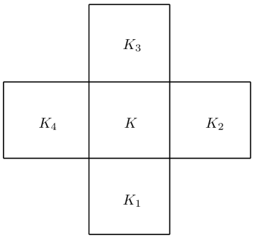
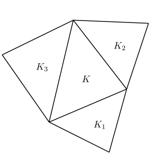
Figure 4.1: Illustration of a rectangular mesh (left) and a triangular mesh (right).

Assume that the 2D spatial domain is partitioned into a mesh ${\mathcal{T}}_{h}$, which can be unstructured and consists of polygonal cells. An illustration of two special meshes is given in Fig. 4.1. Let $K\in\mathcal{T}_{h}$ be a polygonal cell with edges $\mathscr{E}_{K}^{j}$, $j=1,\cdots,N_{K}$, and $K_{j}$ be the adjacent cell which shares the edge $\mathscr{E}_{K}^{j}$ with $K$. We denote by ${\bm{\xi}}_{K}^{(j)}=\big{(}\xi_{1,K}^{(j)},\cdots,\xi_{d,K}^{(j)}\big{)}$ the unit normal vector of $\mathscr{E}_{K}^{j}$ pointing from $K$ to $K_{j}$. The notations $|K|$ and $|{\mathscr{E}}_{K}^{j}|$ are used to denote the area of $K$ and the length of ${\mathscr{E}}_{K}^{j}$, respectively. The time interval is also divided into the mesh $\{t_{0}=0,t_{n+1}=t_{n}+\Delta t_{n},n\geq 0\}$ with the time step-size $\Delta t_{n}$ determined by some CFL condition.

4.1 First-order schemes

We consider the following first-order scheme for the Godunov form (1.4) of the ideal MHD equations

$$\bar{\bf U}_{K}^{n+1}=\bar{\bf U}_{K}^{n}-\frac{\Delta t_{n}}{|K|}\sum_{j=1}^{N_{K}}\left|{\mathscr{E}}_{K}^{j}\right|\hat{\bf F}\big{(}\bar{\bf U}_{K}^{n},\bar{\bf U}_{K_{j}}^{n};{\bm{\xi}}^{(j)}_{K}\big{)}-\Delta t_{n}\big{(}{\rm div}_{K}\bar{\bf B}^{n}\big{)}{\bf S}(\bar{\bf U}^{n}_{K}),$$ (4.1)

where $\bar{\bf U}_{K}^{n}$ is the numerical approximation to the cell average of ${\bf U}({\bf x},t_{n})$ over the cell $K$, and the numerical flux $\hat{\bf F}$ is taken as the HLL flux in (2.29). As a discretization of the Godunov–Powell source, the last term at the right-hand side of (4.1) is a penalty term, with $\mbox{\rm div}_{K}\bar{\bf B}^{n}$ defined by

$$\mbox{\rm div}_{K}\bar{\bf B}^{n}:=\frac{1}{|K|}\sum_{j=1}^{N_{K}}\big{|}{\mathscr{E}}_{K}^{j}\big{|}\left\langle{\bm{\xi}}_{K}^{(j)},\frac{\sigma_{K,j}^{n,+}\bar{\bf B}_{K}^{n}-\sigma_{K,j}^{n,-}\bar{\bf B}_{K_{j}}^{n}}{\sigma_{K,j}^{n,+}-\sigma_{K,j}^{n,-}}\right\rangle,$$ (4.2)

where $\sigma_{K,j}^{n,\pm}:=\sigma^{\pm}(\bar{\bf U}_{K}^{n},\bar{\bf U}_{K_{j}}^{n};{\bm{\xi}}^{(j)}_{K})$. The quantity $\mbox{\rm div}_{K}\bar{\bf B}^{n}$ can be considered as a discrete divergence of magnetic field, because it is a first-order accurate approximation to the left-hand side of

$$\frac{1}{|K|}\sum_{j=1}^{N_{K}}\int_{{\mathscr{E}}_{K}^{j}}\left\langle{\bm{\xi}}_{K}^{(j)},{\bf B}({\bf x},t_{n})\right\rangle ds=\frac{1}{|K|}\int_{K}\nabla\cdot{\bf B}d{\bf x}=0.$$

In the special case of using the LF type fluxes, $\sigma_{K,j}^{n,+}=-\sigma_{K,j}^{n,-}$, then the discrete divergence becomes

$$\mbox{\rm div}_{K}\bar{\bf B}^{n}=\frac{1}{|K|}\sum_{j=1}^{N_{K}}\big{|}{\mathscr{E}}_{K}^{j}\big{|}\left\langle{\bm{\xi}}_{K}^{(j)},\frac{\bar{\bf B}_{K}^{n}+\bar{\bf B}_{K_{j}}^{n}}{2}\right\rangle,$$

which is consistent with the one introduced in [51, 52] on the Cartesian meshes.

The PP property of the scheme (4.1) is shown as follows.

Theorem 4.1.

Let the wave speeds in the HLL flux satisfy (2.30). If $\bar{\bf U}_{K}^{n}\in{\mathcal{G}}$, $\forall K\in{\mathcal{T}}_{h}$, then the solution $\bar{\bf U}^{n+1}_{K}$ of (4.1) belongs to $\mathcal{G}$ for all $K\in{\mathcal{T}}_{h}$ under the CFL-type condition

$$\Delta t_{n}\left(\frac{1}{|K|}\sum_{j=1}^{N_{K}}\big{|}{\mathscr{E}}_{K}^{j}\big{|}\left(-\sigma_{K,j}^{n,-}\right)+\frac{\left|{\rm div}_{K}\bar{\bf B}^{n}\right|}{\sqrt{\bar{\rho}_{K}^{n}}}\right)<1,\quad\forall K\in{\mathcal{T}}_{h}.$$ (4.3)

Proof.

Let ${\bf H}_{K,j}^{n}:={\bf H}(\bar{\bf U}_{K}^{n},\bar{\bf U}_{K_{j}}^{n};{\bm{\xi}}_{K}^{(j)})$. Then the identity (2.31) implies

$$\hat{\bf F}\big{(}\bar{\bf U}_{K}^{n},\bar{\bf U}_{K_{j}}^{n};{\bm{\xi}}^{(j)}_{K}\big{)}=\sigma_{K,j}^{n,-}{\bf H}_{K,j}^{n}+\left\langle{\bm{\xi}}_{K}^{(j)},{\bf F}(\bar{\bf U}_{K}^{n})\right\rangle-\sigma_{K,j}^{n,-}\bar{\bf U}_{K}^{n}.$$ (4.4)

Using (4.4) and the identity

$$\sum_{j=1}^{N_{k}}\big{|}{\mathscr{E}}_{K}^{j}\big{|}{\bm{\xi}}_{K}^{(j)}={\bf 0},$$ (4.5)

one can rewrite the scheme (4.1) as

$$\bar{\bf U}_{K}^{n+1}=\frac{\Delta t_{n}}{|K|}\sum_{j=1}^{N_{K}}\big{|}{\mathscr{E}}_{K}^{j}\big{|}\left(-\sigma_{K,j}^{n,-}\right){\bf H}_{K,j}^{n}+(1-\lambda_{K})\bar{\bf U}_{K}^{n}-\Delta t_{n}\big{(}{\rm div}_{K}\bar{\bf B}^{n}\big{)}{\bf S}(\bar{\bf U}^{n}_{K}),$$ (4.6)

where $\lambda_{K}:=\frac{\Delta t_{n}}{|K|}\sum_{j=1}^{N_{K}}\big{|}{\mathscr{E}}_{K}^{j}\big{|}\big{(}-\sigma_{K,j}^{n,-}\big{)}\in[0,1).$ Thanks to Theorem 2.2, we have ${\bf H}_{K,j}^{n}\in{\mathcal{G}}_{\rho}$ and for any ${\bf v}^{*},{\bf B}^{*}\in{\mathbb{R}}^{3}$,

$${\bf H}_{K,j}^{n}\cdot{\bf n}^{*}+\frac{|{\bf B}^{*}|^{2}}{2}\geq-\frac{{\bf v}^{*}\cdot{\bf B}^{*}}{\sigma_{K,j}^{n,+}-\sigma_{K,j}^{n,-}}\left\langle{\bm{\xi}}_{K}^{(j)},\bar{\bf B}_{K_{j}}^{n}-\bar{\bf B}_{K}^{n}\right\rangle.$$ (4.7)

Since ${\bf H}_{K,j}^{n}\in{\mathcal{G}}_{\rho}$ and the first component of ${\bf S}(\bar{\bf U}^{n}_{K})$ is zero, we have $\bar{\rho}^{n+1}_{K}\geq(1-\lambda_{K})\bar{\rho}^{n}_{K}>0$. For any ${\bf v}^{*},{\bf B}^{*}\in\mathbb{R}^{3}$, using (2.24) we derive from (4.6) that

$$\bar{\bf U}_{K}^{n+1}\cdot{\bf n}^{*}+\frac{|{\bf B}^{*}|^{2}}{2}=\Pi_{1}+\Pi_{2},$$

where

$$\Pi_{1} :=\frac{\Delta t_{n}}{|K|}\sum_{j=1}^{N_{K}}\big{|}{\mathscr{E}}_{K}^{j}\big{|}\left(-\sigma_{K,j}^{n,-}\right)\left({\bf H}_{K,j}^{n}\cdot{\bf n}^{*}+\frac{|{\bf B}^{*}|^{2}}{2}\right)+\Delta t_{n}\big{(}\mbox{\rm div}_{K}\bar{\bf B}^{n}\big{)}\big{(}{\bf v}^{*}\cdot{\bf B}^{*}\big{)},$$

$$\Pi_{2} :=(1-\lambda_{K})\left(\bar{\bf U}_{K}^{n}\cdot{\bf n}^{*}+\frac{|{\bf B}^{*}|^{2}}{2}\right)-\Delta t_{n}\big{(}{\rm div}_{K}\bar{\bf B}^{n}\big{)}(\bar{\bf v}_{K}^{n}-{\bf v}^{*})\cdot(\bar{\bf B}_{K}^{n}-{\bf B}^{*}).$$

Let us estimate the lower bounds of $\Pi_{1}$ and $\Pi_{2}$ respectively. Using (4.7) and (4.5) gives

$$\Pi_{1} \overset{\eqref{eq:Hnstar}}{\geq}\frac{\Delta t_{n}}{|K|}\sum_{j=1}^{N_{K}}\big{|}{\mathscr{E}}_{K}^{j}\big{|}\sigma_{K,j}^{n,-}\frac{\big{\langle}{\bm{\xi}}_{K}^{(j)},\bar{\bf B}_{K_{j}}^{n}-\bar{\bf B}_{K}^{n}\big{\rangle}}{\sigma_{K,j}^{n,+}-\sigma_{K,j}^{n,-}}\big{(}{\bf v}^{*}\cdot{\bf B}^{*}\big{)}+\Delta t_{n}\big{(}\mbox{\rm div}_{K}\bar{\bf B}^{n}\big{)}\big{(}{\bf v}^{*}\cdot{\bf B}^{*}\big{)}$$

$$\overset{\eqref{eq:DefDisDivB}}{=}\frac{\Delta t_{n}}{|K|}\sum_{j=1}^{N_{K}}\big{|}{\mathscr{E}}_{K}^{j}\big{|}\left(\sigma_{K,j}^{n,-}\frac{\big{\langle}{\bm{\xi}}_{K}^{(j)},\bar{\bf B}_{K_{j}}^{n}-\bar{\bf B}_{K}^{n}\big{\rangle}}{\sigma_{K,j}^{n,+}-\sigma_{K,j}^{n,-}}+\left\langle{\bm{\xi}}_{K}^{(j)},\frac{\sigma_{K,j}^{n,+}\bar{\bf B}_{K}^{n}-\sigma_{K,j}^{n,-}\bar{\bf B}_{K_{j}}^{n}}{\sigma_{K,j}^{n,+}-\sigma_{K,j}^{n,-}}\right\rangle\right)\big{(}{\bf v}^{*}\cdot{\bf B}^{*}\big{)}$$

$$=\frac{\Delta t_{n}}{|K|}\sum_{j=1}^{N_{K}}\big{|}{\mathscr{E}}_{K}^{j}\big{|}\left\langle{\bm{\xi}}_{K}^{(j)},\bar{\bf B}_{K}^{n}\right\rangle\big{(}{\bf v}^{*}\cdot{\bf B}^{*}\big{)}\overset{\eqref{eq:sumxi0}}{=}0.$$

It follows from (2.25) that

$$\Pi_{2} \geq(1-\lambda_{K})\left(\bar{\bf U}_{K}^{n}\cdot{\bf n}^{*}+\frac{|{\bf B}^{*}|^{2}}{2}\right)-\Delta t_{n}\frac{\left|{\rm div}_{K}\bar{\bf B}^{n}\right|}{\sqrt{\bar{\rho}^{n}_{K}}}\Big{|}\sqrt{\bar{\rho}^{n}_{K}}(\bar{\bf v}_{K}^{n}-{\bf v}^{*})\cdot(\bar{\bf B}_{K}^{n}-{\bf B}^{*})\Big{|}$$

$$\overset{\eqref{eq:widelyusedIEQ}}{\geq}\left(1-\lambda_{K}-\Delta t_{n}\frac{\left|{\rm div}_{K}\bar{\bf B}^{n}\right|}{\sqrt{\bar{\rho}^{n}_{K}}}\right)\left(\bar{\bf U}_{K}^{n}\cdot{\bf n}^{*}+\frac{|{\bf B}^{*}|^{2}}{2}\right)>0.$$

Therefore, $\bar{\bf U}_{K}^{n+1}\cdot{\bf n}^{*}+\frac{|{\bf B}^{*}|^{2}}{2}>0$, $\forall{\bf v}^{*},{\bf B}^{*}\in\mathbb{R}^{3}$.

Hence $\bar{\bf U}_{K}^{n+1}\in\mathcal{G}$ by Lemma 2.1. $\blacksquare$

It is worth emphasizing that the penalty term is crucial for guaranteeing the PP property of the scheme (4.1). While the scheme (4.1) without this term reduces to the 2D HLL scheme for the conservative MHD system (1.1), specifically,

$$\bar{\bf U}_{K}^{n+1}=\bar{\bf U}_{K}^{n}-\frac{\Delta t_{n}}{|K|}\sum_{j=1}^{N_{K}}\big{|}{\mathscr{E}}_{K}^{j}\big{|}\hat{\bf F}\big{(}\bar{\bf U}_{K}^{n},\bar{\bf U}_{K_{j}}^{n};{\bm{\xi}}^{(j)}_{K}\big{)}.$$ (4.8)

For the LF flux, the analysis in [51] on Cartesian meshes showed that the scheme (4.8) is generally not PP, unless a discrete divergence-free (DDF) condition is satisfied. We find that, on a general mesh ${\mathcal{T}}_{h}$, the corresponding DDF condition is

$$\mbox{\rm div}_{K}\bar{\bf B}^{n}=0,\quad\forall K\in{\mathcal{T}}_{h}.$$ (4.9)

As a direct consequence of Theorem 4.1, we immediately have the following corollary.

Corollary 4.1.

Let the wave speeds in the HLL flux satisfy (2.30). If $\bar{\bf U}_{K}^{n}\in{\mathcal{G}}$, $\forall K\in{\mathcal{T}}_{h}$, and satisfy the DDF condition (4.9), then under the CFL condition

$$\frac{\Delta t_{n}}{|K|}\sum_{j=1}^{N_{K}}\big{|}{\mathscr{E}}_{K}^{j}\big{|}\left(-\sigma_{K,j}^{n,-}\right)<1,\quad\forall K\in{\mathcal{T}}_{h},$$

the solution $\bar{\bf U}^{n+1}_{K}$ of (4.8) belongs to $\mathcal{G}$ for all $K\in{\mathcal{T}}_{h}$.

If ${\mathcal{T}}_{h}$ is a Cartesian mesh and the numerical flux $\hat{\bf F}$ is taken as the global LF flux, then the scheme (4.8) preserves the DDF condition (4.9) provided that the DDF condition is satisfied by the initial data [51]. It was also shown in [51] that even slightly violating the DDF condition can cause the failure of the scheme (4.8) to preserve the positivity of pressure. Unfortunately, on general meshes the scheme (4.8) does not necessarily preserve the DDF condition (4.9), and it is generally not PP.

4.2 High-order schemes

We are now in the position to discuss provably PP high-order schemes for the multidimensional ideal MHD. We mainly focus on the PP high-order DG methods, keeping in mind that the analysis and framework also apply to high-order finite volume schemes.

4.2.1 Locally divergence-free schemes

We first propose locally divergence-free schemes for the modified MHD system (1.4), as they are the base schemes of our PP high-order schemes presented later. Towards achieving high-order spatial accuracy, the exact solution ${\bf U}({\bf x},t_{n})$ is approximated with a discontinuous piecewise polynomial function ${\bf U}_{h}^{n}({\bf x})$, which is sought in the locally divergence-free DG space [34]

$${\mathbb{V}}_{h}^{k}=\left\{{\bf u}=(u_{1},\cdots,u_{8})^{\top}~{}\Big{|}~{}u_{\ell}\big{|}_{K}\in{\mathbb{P}}^{k}(K),\forall\ell,~{}\sum_{i=1}^{d}\frac{\partial u_{4+i}}{\partial{x_{i}}}\bigg{|}_{K}=0,~{}\forall K\in{\mathcal{T}}_{h}\right\},$$

where ${\mathbb{P}}^{k}(K)$ is the space of polynomials in $K$ of degree at most $k$.

Our ${\mathbb{P}}^{k}$-based locally divergence-free DG method is obtained by proper discretization of the Godunov form (1.4). Specifically, our DG solution ${\bf U}_{h}^{n}\in{\mathbb{V}}_{h}^{k}$ is explicitly evolved by

$$\begin{split}&\int_{K}{\bf u}\cdot\frac{{\bf U}_{h}^{n+1}-{\bf U}_{h}^{n}}{\Delta t_{n}}dxdy=\int_{K}\nabla{\bf u}\cdot{\bf F}({\bf U}_{h}^{n})d{\bf x}\\ &\quad-\sum_{j=1}^{N_{K}}\int_{{\mathscr{E}}_{K}^{j}}{\bf u}^{{\rm int}(K)}\cdot\bigg{\{}\hat{\bf F}\left({\bf U}_{h}^{n,{\rm int}(K)},{\bf U}_{h}^{n,{\rm ext}(K)};{\bm{\xi}}^{(j)}_{K}\right)\\ &\qquad-\left[\eta_{K}({\bf x})\left\langle{\bm{\xi}}^{(j)}_{K},{\bf B}_{h}^{n,{\rm ext}(K)}-{\bf B}_{h}^{n,{\rm int}(K)}\right\rangle{\bf S}\big{(}{\bf U}_{h}^{n,{\rm int}(K)}\big{)}\right]\bigg{\}}ds,\quad\forall{\bf u}\in{\mathbb{V}}_{h}^{k},\end{split}$$ (4.10)

where the numerical flux $\hat{\bf F}$ is taken as the HLL flux in (2.29), and the factor

$$\eta_{K}({\bf x}):=\frac{\sigma^{-}\big{(}{\bf U}_{h}^{n,{\rm int}(K)},{\bf U}_{h}^{n,{\rm ext}(K)};{\bm{\xi}}^{(j)}_{K}\big{)}}{\sigma^{+}\big{(}{\bf U}_{h}^{n,{\rm int}(K)},{\bf U}_{h}^{n,{\rm ext}(K)};{\bm{\xi}}^{(j)}_{K}\big{)}-\sigma^{-}\big{(}{\bf U}_{h}^{n,{\rm int}(K)},{\bf U}_{h}^{n,{\rm ext}(K)};{\bm{\xi}}^{(j)}_{K}\big{)}},\quad\forall{\bf x}\in{\mathscr{E}}_{K}^{j}.$$

Here the superscripts “${\rm int}(K)$” and “${\rm ext}(K)$” indicate that the associated limits at the interface ${\mathscr{E}}_{K}^{j}$ are taken from the interior and exterior of $K$, respectively. The term inside the bracket in (4.10) is a penalty term discretized from the Godunov–Powell source term. The factor $\eta_{K}$ is carefully devised in an upwind manner according to the local wave speeds in the HLL flux. This is motivated from our theoretical analysis, and is very important for achieving the provably PP property, as we will see the proof of Theorem 4.2 and Remark 4.3. If the LF flux is employed, i.e., $\sigma^{-}=-\sigma^{+}$, then $\eta_{K}({\bf x})\equiv-\frac{1}{2}$, and the penalty term reduces to the one used in [52].

In the practical computations, the boundary and element integrals at the right-hand side of (4.10) are discretized by certain quadratures of sufficiently high order accuracy (specifically, the algebraic degree of accuracy should be at least $2k$). For example, we can employ the Gauss quadrature with $Q=k+1$ points for the boundary integral:

$$\begin{split}&\int_{{\mathscr{E}}_{K}^{j}}{\bf u}^{{\rm int}(K)}\cdot\bigg{[}\hat{\bf F}\left({\bf U}_{h}^{n,{\rm int}(K)},{\bf U}_{h}^{n,{\rm ext}(K)};{\bm{\xi}}^{(j)}_{K}\right)\\ &\qquad-\eta_{K}({\bf x})\left\langle{\bm{\xi}}^{(j)}_{K},{\bf B}_{h}^{n,{\rm ext}(K)}-{\bf B}_{h}^{n,{\rm int}(K)}\right\rangle{\bf S}\big{(}{\bf U}_{h}^{n,{\rm int}(K)}\big{)}\bigg{]}ds\end{split}$$

$$\begin{split}&\quad\approx|{\mathscr{E}}_{K}^{j}|\sum_{q=1}^{Q}\omega_{q}{\bf u}^{{\rm int}(K)}({\bf x}_{K}^{(jq)})\cdot\bigg{[}\hat{\bf F}\left({\bf U}_{h}^{n,{\rm int}(K)}({\bf x}_{K}^{(jq)}),{\bf U}_{h}^{n,{\rm ext}(K)}({\bf x}_{K}^{(jq)});{\bm{\xi}}^{(j)}_{K}\right)\\ &\qquad-\eta_{K}({\bf x}_{K}^{(jq)})\left\langle{\bm{\xi}}^{(j)}_{K},{\bf B}_{h}^{n,{\rm ext}(K)}({\bf x}_{K}^{(jq)})-{\bf B}_{h}^{n,{\rm int}(K)}({\bf x}_{K}^{(jq)})\right\rangle{\bf S}\left({\bf U}_{h}^{n,{\rm int}(K)}({\bf x}_{K}^{(jq)})\right)\bigg{]},\end{split}$$

where $\{{\bf x}_{K}^{(jq)}\}_{1\leq q\leq Q}$ are the quadrature points on the interface ${\mathscr{E}}_{K}^{j}$, and $\{\omega_{q}\}_{1\leq q\leq Q}$ are the associated weights.

Let

$${\bf U}_{h}^{n}\big{|}_{K}=:{\bf U}_{K}^{n}({\bf x}),$$

and its cell average over $K$ be $\bar{\bf U}_{K}^{n}$. Then we can obtain from (4.10) the evolution equations for the cell averages $\{\bar{\bf U}_{K}^{n}\}$ as follows

$$\bar{\bf U}_{K}^{n+1}=\bar{\bf U}_{K}^{n}+\Delta t_{n}{\bf L}_{K}({\bf U}_{h}^{n}),$$ (4.11)

where

$$\begin{split}{\bf L}_{K}({\bf U}_{h}^{n})&:=-\frac{1}{|K|}\sum_{j=1}^{N_{K}}\sum_{q=1}^{Q}|{\mathscr{E}}_{K}^{j}|\omega_{q}\bigg{[}\hat{\bf F}\left({\bf U}_{h}^{n,{\rm int}(K)}({\bf x}_{K}^{(jq)}),{\bf U}_{h}^{n,{\rm ext}(K)}({\bf x}_{K}^{(jq)});{\bm{\xi}}^{(j)}_{K}\right)\\ &-\eta_{K}({\bf x}_{K}^{(jq)})\left\langle{\bm{\xi}}^{(j)}_{K},{\bf B}_{h}^{n,{\rm ext}(K)}({\bf x}_{K}^{(jq)})-{\bf B}_{h}^{n,{\rm int}(K)}({\bf x}_{K}^{(jq)})\right\rangle{\bf S}\left({\bf U}_{h}^{n,{\rm int}(K)}({\bf x}_{K}^{(jq)})\right)\bigg{]}.\end{split}$$

The scheme (4.11) can also be derived from a finite volume method for (1.4), if the approximate function ${\bf U}_{h}^{n}$ in (4.11) is reconstructed from $\{\bar{\bf U}_{K}^{n}\}$ by using a locally divergence-free reconstruction approach (cf. [66, 58]) such that ${\bf U}_{h}^{n}\in{\mathbb{V}}_{h}^{k}$.

If choosing $k=0$, the above finite volume and DG schemes reduce to the first-order scheme (4.1), whose PP property has been proven in Theorem 4.1. If taking $k\geq 1$, the above high-order accurate DG and finite volume schemes are generally not PP. However, we find that these locally divergence-free schemes have the weak positivity, that is, they can be rendered provably PP by a simple limiting procedure, as demonstrated in the following. Note that the standard multidimensional DG schemes does not have the weak positivity, even if the locally divergence-free element is used.

4.2.2 Positivity-preserving schemes

We first assume that there exists a special 2D quadrature on each cell $K\in{\mathcal{T}}_{h}$ satisfying:

• The quadrature rule is with positive weights and exact for integrals of polynomials of degree up to $k$ on the cell $K$.

• The set of the quadrature points, denoted by ${\mathbb{S}}_{K}$, must include all the Gauss quadrature points ${\bf x}_{K}^{(jq)}$, $j=1,\dots,N_{K}$, $q=1,\dots,Q$, on the cell interface.

In other words, we would like to have a special quadrature such that

$$\frac{1}{|K|}\int_{K}u({\bf x})d{\bf x}=\sum_{j=1}^{N_{K}}\sum_{q=1}^{Q}\varpi_{jq}u({\bf x}_{K}^{(jq)})+\sum_{q=1}^{\widetilde{Q}}\widetilde{\varpi}_{q}u(\widetilde{\bf x}_{K}^{(q)}),\quad\forall u\in{\mathbb{P}}^{k}(K),$$ (4.12)

where $\{\widetilde{\bf x}_{K}^{(q)}\}$ are the other (possible) quadrature nodes in $K$, and the quadrature weights $\varpi_{jq},\widetilde{\varpi}_{q}$ are positive and satisfy $\sum_{j=1}^{N_{K}}\sum_{q=1}^{Q}\varpi_{jq}+\sum_{q=1}^{\widetilde{Q}}\widetilde{\varpi}_{q}=1.$ For rectangular cells, such a quadrature was constructed in [62, 63] by tensor products of Gauss quadrature and Gauss–Lobatto quadrature. For triangular cells, it can be constructed by a Dubinar transform from rectangles to triangles [65]. For more general polygonal cells, one can always decompose the polygons into non-overlapping triangles, and then build the above quadrature rule by gathering those on the small triangles; see, for example, [47, 22]. An illustration of the special quadrature on rectangle and triangle for $k=2$ is shown in Fig. 4.2, where the (red) solid points are $\{{\bf x}_{K}^{(jq)}\}$ and the (blue) hollow circles denote $\{\widetilde{\bf x}_{K}^{(q)}\}$. We remark that such a special quadrature is not employed for computing any integral, but only used in the PP limiter and theoretical analysis as it decomposes the cell average into a convex combination of the desired point values.

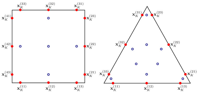
Figure 4.2: Illustration of the quadrature (4.12) on a rectangular cell (left) and a triangular cell (right) for $k=2$. The (red) solid points are $\{{\bf x}_{K}^{(jq)}\}$ and the (blue) hollow circles denote $\{\widetilde{\bf x}_{K}^{(q)}\}$; all of them constitute the point set ${\mathbb{S}}_{K}$.

Based on the above special quadrature and the high-order locally divergence-free schemes in Section 4.2.1, our provably PP high-order DG and finite volume schemes are constructed as follows. The rigorous proof of the PP property is very technical and will be presented later.

Step 0. Initialization. After setting $t=0$ and $n=0$, we compute the cell averages $\{\bar{\bf U}_{K}^{0}\}$ and the polynomial functions $\{{\bf U}_{K}^{0}({\bf x})\}$ by a local $L^{2}$-projection of the initial data onto ${\mathbb{V}}_{h}^{k}$, so that $\bar{\bf U}_{K}^{0}\in{\mathcal{G}}$ is ensured by the convexity of $\mathcal{G}$, and ${\bf U}_{h}^{0}\in{\mathbb{V}}_{h}^{k}$ is also guaranteed.

Step 1. Given admissible cell-averaged solution $\big{\{}\bar{\bf U}_{K}^{n}\big{\}}$ and ${\bf U}_{h}^{n}\in{\mathbb{V}}_{h}^{k}$, perform the PP limiting procedure. The PP limiter [13] is employed to modify the polynomials $\big{\{}{\bf U}_{K}^{n}({\bf x})\big{\}}$, such that the modified polynomials $\big{\{}\widetilde{\bf U}_{K}^{n}({\bf x})\big{\}}$ satisfy

$$\widetilde{\bf U}_{K}^{n}({\bf x})\in{\mathcal{G}},\quad\forall{\bf x}\in{\mathbb{S}}_{K}:=\left\{\widetilde{\bf x}_{K}^{(q)}\right\}_{1\leq q\leq\widetilde{Q}}\bigcup\left\{{\bf x}_{K}^{(jq)}\right\}_{1\leq j\leq N_{K},1\leq q\leq Q}.$$ (4.13)

For readers’ convenience, the PP limiter is briefly reviewed in Appendix B. Let $\widetilde{\bf U}_{h}^{n}({\bf x})$ be the (discontinuous) piecewise polynomial function corresponding to $\widetilde{\bf U}_{K}^{n}({\bf x})$. Note that the limited function $\widetilde{\bf U}_{h}^{n}\in{\mathbb{V}}_{h}^{k}$, since the PP limiter only involves certain local convex combination of ${\bf U}_{K}^{n}({\bf x})$ and its cell average over $K$.

Step 2. Update the cell averages by the scheme

$$\bar{\bf U}_{K}^{n+1}=\bar{\bf U}_{K}^{n}+\Delta t_{n}{\bf L}_{K}(\widetilde{\bf U}_{h}^{n}),$$ (4.14)

As will be shown in Theorem 4.2, because of the weak positivity of our locally divergence-free schemes, the PP limiting procedure in Step 1 can ensure $\bar{\bf U}_{K}^{n+1}\in{\mathcal{G}}$, which meets the requirement of performing the PP limiting procedure in the next time-forward step.

Step 3. Build the piecewise polynomial function ${\bf U}_{h}^{n+1}$. For our $\mathbb{P}^{k}$-based DG method $({k}\geq 1)$, the high-order “moments” of the polynomials $\{{\bf U}_{K}^{n+1}({\bf x})\}$ are evolved by (4.10) with ${\bf U}_{h}^{n}$ replaced with $\widetilde{\bf U}_{h}^{n}$. For a high-order finite volume scheme, the approximate solution polynomials $\{{\bf U}_{K}^{n+1}({\bf x})\}$ are reconstructed from the cell averages $\big{\{}\bar{\bf U}_{K}^{n+1}\big{\}}$ by a locally divergence-free method such that ${\bf U}_{h}^{n+1}\in{\mathbb{V}}_{h}^{k}$. We here omit the details, because these does not affect the PP property of the schemes.

Step 4. Set $t_{n+1}=t_{n}+\Delta t_{n}$. If $t_{n+1}<T$, assign $n\leftarrow n+1$ and go to Step 1, where $\bar{\bf U}_{K}^{n+1}\in{\mathcal{G}}$ has been guaranteed in Step 2; otherwise, output results.

Now, we give the proof of the PP property of the above schemes, i.e., prove that the cell average $\bar{\bf U}_{K}^{n+1}$ computed by the scheme (4.14) always stays $\mathcal{G}$ under the condition (4.13). It is worth emphasizing that the locally divergence-free spatial discretization and the penalty term in (4.10) are crucial for achieving the provably PP scheme, as will be seen from the proof of Theorem 4.2.

To shorten the notations, we define

$${\bf U}^{{\rm int}(K)}_{jq}:=\widetilde{\bf U}_{h}^{n,{\rm int}(K)}({\bf x}_{K}^{(jq)}),\qquad{\bf U}^{{\rm ext}(K)}_{jq}:=\widetilde{\bf U}_{h}^{n,{\rm ext}(K)}({\bf x}_{K}^{(jq)}),$$

where the dependence on $n$ is omitted. Let

$$\sigma_{jq}^{K,\pm}:=\sigma^{\pm}\big{(}{\bf U}_{jq}^{{\rm int}(K)},{\bf U}_{jq}^{{\rm ext}(K)};{\bm{\xi}}^{(j)}_{K}\big{)}.$$

For $\forall K\in{\mathcal{T}}_{h}$, we define

$$\begin{split}&\widehat{\alpha}_{jq}^{{\rm int}(K)}:={\mathscr{C}}({\bf U}_{jq}^{{\rm int}(K)};{\bm{\xi}}_{K}^{(j)})+\frac{2}{|\partial K|}\sum_{i=1}^{N_{K}}|{\mathscr{E}}_{K}^{i}|\frac{|{\bf B}_{jq}^{{\rm int}(K)}-{\bf B}_{iq}^{{\rm int}(K)}|}{\sqrt{\rho_{jq}^{{\rm int}(K)}}+\sqrt{\rho_{iq}^{{\rm int}(K)}}}\\ &+\max\left\{\big{\langle}{\bm{\xi}}^{(j)}_{K},{\bf v}^{{\rm int}(K)}_{jq}\big{\rangle},\frac{1}{|\partial K|}\sum_{i=1}^{N_{K}}|{\mathscr{E}}_{K}^{i}|\left\langle{\bm{\xi}}^{(j)}_{K}-{\bm{\xi}}^{(i)}_{K},\frac{\sqrt{\rho_{jq}^{{\rm int}(K)}}{\bf v}_{jq}^{{\rm int}(K)}+\sqrt{\rho_{iq}^{{\rm int}(K)}}{\bf v}_{iq}^{{\rm int}(K)}}{\sqrt{\rho_{jq}^{{\rm int}(K)}}+\sqrt{\rho_{iq}^{{\rm int}(K)}}}\right\rangle\right\},\end{split}$$

with $|\partial K|:=\sum_{i=1}^{N_{K}}|{\mathscr{E}}_{K}^{i}|$ denoting the circumference of the cell $K$.

Theorem 4.2.

Let the wave speeds in the HLL flux satisfy (2.30). If the polynomial vectors $\{\widetilde{\bf U}_{K}^{n}({\bf x})\}$ are locally divergence-free and satisfy the condition (4.13), then the scheme (4.14) preserves $\bar{\bf U}_{K}^{n+1}\in{\mathcal{G}}$ under the CFL-type condition

$$\Delta t_{n}\frac{|{\mathscr{E}}_{K}^{j}|}{|K|}\alpha_{jq}^{K}<\frac{\varpi_{jq}}{\omega_{q}},\qquad\forall K\in{\mathcal{T}}_{h},~{}1\leq j\leq N_{K},~{}1\leq q\leq Q,$$ (4.15)

with

$$\alpha_{jq}^{K}:=\widehat{\alpha}_{jq}^{{\rm int}(K)}-\sigma_{jq}^{K,-}-\eta_{K}\big{(}{\bf x}_{K}^{(jq)}\big{)}\Big{(}{\rho_{jq}^{{\rm int}(K)}}\Big{)}^{-\frac{1}{2}}\left|\big{\langle}{\bm{\xi}}_{K}^{(j)},{\bf B}_{jq}^{{\rm int}(K)}-{\bf B}_{jq}^{{\rm ext}(K)}\big{\rangle}\right|.$$ (4.16)

Note that $\sigma_{jq}^{K,-}\leq 0$ and $-1\leq\eta_{K}\big{(}{\bf x}_{K}^{(jq)}\big{)}\leq 0$. The last term in (4.16) is relatively small compared to the maximum signal speed, and thus does not cause strict restriction on the time step-size; see the detailed justification and numerical evidence in [52].

We now present the proof of Theorem 4.2.

Proof.

Recalling the identity (2.31) and Theorem 2.2, one has

$$\begin{split}&\hat{\bf F}\big{(}{\bf U}_{jq}^{{\rm int}(K)},{\bf U}_{jq}^{{\rm ext}(K)};{\bm{\xi}}^{(j)}_{K}\big{)}=\sigma_{jq}^{K,-}{\bf H}_{jq}^{K}+\left\langle{\bm{\xi}}_{K}^{(j)},{\bf F}({\bf U}_{jq}^{{\rm int}(K)})\right\rangle-\sigma_{jq}^{K,-}{\bf U}_{jq}^{{\rm int}(K)}\\ &=\big{(}\widehat{\alpha}_{jq}^{{\rm int}(K)}-\sigma_{jq}^{K,-}\big{)}{\bf U}_{jq}^{{\rm int}(K)}-\left(\widehat{\alpha}_{jq}^{{\rm int}(K)}{\bf U}_{jq}^{{\rm int}(K)}-\big{\langle}{\bm{\xi}}_{K}^{(j)},{\bf F}({\bf U}_{jq}^{{\rm int}(K)})\big{\rangle}\right)+\sigma_{jq}^{K,-}{\bf H}_{jq}^{K},\end{split}$$

where ${\bf H}_{jq}^{K}:={\bf H}({\bf U}_{jq}^{{\rm int}(K)},{\bf U}_{jq}^{{\rm ext}(K)};{\bm{\xi}}_{K}^{(j)})\in{\mathcal{G}}_{\rho}$ and for $\forall{\bf v}^{*},{\bf B}^{*}\in\mathbb{R}^{3}$,

$${\bf H}_{jq}^{K}\cdot{\bf n}^{*}+\frac{|{\bf B}^{*}|^{2}}{2}\geq-\frac{{\bf v}^{*}\cdot{\bf B}^{*}}{\sigma_{jq}^{K,+}-\sigma_{jq}^{K,-}}\left\langle{\bm{\xi}}_{K}^{(j)},{\bf B}_{jq}^{{\rm ext}(K)}-{\bf B}_{jq}^{{\rm int}(K)}\right\rangle.$$ (4.17)

Plugging the above formula of $\hat{\bf F}$ into (4.14), we can rewrite the scheme (4.14) as

$$\bar{\bf U}_{K}^{n+1}=\bar{\bf U}_{K}^{n}+{\bf\Xi}_{1}+{\bf\Xi}_{2}+{\bf\Xi}_{3}+{\bf\Xi}_{4},$$ (4.18)

with

$${\bf\Xi}_{1}:=\frac{\Delta t_{n}}{|K|}\sum_{j=1}^{N_{K}}\sum_{q=1}^{Q}|{\mathscr{E}}_{K}^{j}|\omega_{q}\left(\sigma_{jq}^{K,-}-\widehat{\alpha}_{jq}^{{\rm int}(K)}\right){\bf U}_{jq}^{{\rm int}(K)}$$

$${\bf\Xi}_{2}:=\frac{\Delta t_{n}}{|K|}\sum_{j=1}^{N_{K}}\sum_{q=1}^{Q}|{\mathscr{E}}_{K}^{j}|\omega_{q}\left(\widehat{\alpha}_{jq}^{{\rm int}(K)}{\bf U}_{jq}^{{\rm int}(K)}-\big{\langle}{\bm{\xi}}_{K}^{(j)},{\bf F}({\bf U}_{jq}^{{\rm int}(K)})\big{\rangle}\right),$$

$${\bf\Xi}_{3}:=\frac{\Delta t_{n}}{|K|}\sum_{j=1}^{N_{K}}\sum_{q=1}^{Q}|{\mathscr{E}}_{K}^{j}|\omega_{q}\left(-\sigma_{jq}^{K,-}\right){\bf H}_{jq}^{K},$$

$${\bf\Xi}_{4}:=\frac{\Delta t_{n}}{|K|}\sum_{j=1}^{N_{K}}\sum_{q=1}^{Q}\big{|}{\mathscr{E}}_{K}^{j}\big{|}\omega_{q}\eta_{K}\big{(}{\bf x}_{K}^{(jq)}\big{)}\left\langle{\bm{\xi}}_{K}^{(j)},{\bf B}_{jq}^{{\rm ext}(K)}-{\bf B}_{jq}^{{\rm int}(K)}\right\rangle{\bf S}\big{(}{\bf U}_{jq}^{{\rm int}(K)}\big{)}.$$

For $1\leq q\leq Q$, let

$$\overline{{\bf U}}^{{\rm int}(K)}_{q}:=\frac{1}{\sum\limits_{j=1}^{N_{K}}\big{|}{\mathscr{E}}_{K}^{j}\big{|}\widehat{\alpha}_{jq}^{{\rm int}(K)}}\sum_{j=1}^{N_{K}}|{\mathscr{E}}_{K}^{j}|\left(\widehat{\alpha}_{jq}^{{\rm int}(K)}{\bf U}_{jq}^{{\rm int}(K)}-\big{\langle}{\bm{\xi}}_{K}^{(j)},{\bf F}({\bf U}_{jq}^{{\rm int}(K)})\big{\rangle}\right),$$

then ${\bf\Xi}_{2}$ can be reformulated as

$${\bf\Xi}_{2}=\frac{\Delta t_{n}}{|K|}\sum_{q=1}^{Q}\omega_{q}\left(\sum_{j=1}^{N_{K}}|{\mathscr{E}}_{K}^{j}|\widehat{\alpha}_{jq}^{{\rm int}(K)}\right)\overline{{\bf U}}^{{\rm int}(K)}_{q}.$$ (4.19)

Thanks to Theorem 2.1 and Eq. (4.5), we have, for all $1\leq q\leq Q$, $\overline{{\bf U}}^{{\rm int}(K)}_{q}\in{\mathcal{G}}_{\rho}$ and

$$\overline{\bf U}^{{\rm int}(K)}_{q}\cdot{\bf n}^{*}+\frac{|{\bf B}^{*}|^{2}}{2}\geq-\frac{{\bf v}^{*}\cdot{\bf B}^{*}}{{\sum\limits_{j=1}^{N_{K}}{|{\mathscr{E}}_{K}^{j}|\widehat{\alpha}_{jq}^{{\rm int}(K)}}}}\sum_{j=1}^{N_{K}}|{\mathscr{E}}_{K}^{j}|\big{\langle}{\bm{\xi}}^{(j)}_{K},{\bf B}_{jq}^{{\rm int}(K)}\big{\rangle},\quad\forall{\bf v}^{*},{\bf B}^{*}\in{\mathbb{R}}^{3}.$$

Note $\sum_{j=1}^{N_{K}}|{\mathscr{E}}_{K}^{j}|\widehat{\alpha}_{jq}^{{\rm int}(K)}>0$ as indicated in Remark 2.1. Therefore, ${\bf\Xi}_{2}\in{\mathcal{G}}_{\rho}$, and

$${\Pi}_{2} :=\frac{\Delta t_{n}}{|K|}\sum_{q=1}^{Q}\omega_{q}\left(\sum_{j=1}^{N_{K}}|{\mathscr{E}}_{K}^{j}|\widehat{\alpha}_{jq}^{{\rm int}(K)}\right)\left(\overline{{\bf U}}^{{\rm int}(K)}_{q}\cdot{\bf n}^{*}+\frac{|{\bf B}^{*}|^{2}}{2}\right)$$ (4.20)

$$\geq-\frac{\Delta t_{n}}{|K|}\big{(}{\bf v}^{*}\cdot{\bf B}^{*}\big{)}\sum_{q=1}^{Q}\omega_{q}\sum_{j=1}^{N_{K}}|{\mathscr{E}}_{K}^{j}|\big{\langle}{\bm{\xi}}^{(j)}_{K},{\bf B}_{jq}^{{\rm int}(K)}\big{\rangle}.$$

It follows that

$$\Pi_{2} \geq-\frac{\Delta t_{n}}{|K|}\big{(}{\bf v}^{*}\cdot{\bf B}^{*}\big{)}\sum_{j=1}^{N_{K}}\int_{{\mathscr{E}}_{K}^{j}}\big{\langle}{\bm{\xi}}^{(j)}_{K},\widetilde{\bf B}_{K}^{n}\big{\rangle}ds$$ (4.21)

$$=-\frac{\Delta t_{n}}{|K|}\big{(}{\bf v}^{*}\cdot{\bf B}^{*}\big{)}\int_{K}\big{(}\nabla\cdot\widetilde{\bf B}_{K}^{n}\big{)}d{\bf x}=0,$$

where we have sequentially used the exactness of the $Q$-point quadrature rule on each interface for polynomials of degree up to $k$, Green’s theorem and the locally divergence-free property of the polynomial vector $\widetilde{\bf B}_{K}^{n}({\bf x})$.

Now, we first show $\bar{\rho}_{K}^{n+1}>0$. Recalling that the first component of ${\bf S}({\bf U})$ is zero, we know that the first component of ${\bf\Xi}_{4}$ is zero. Since ${\bf\Xi}_{2}\in{\mathcal{G}}_{\rho}$ and ${\bf H}_{jq}^{K}\in{\mathcal{G}}_{\rho}$, $1\leq j\leq N_{K}$, $1\leq q\leq Q$, we deduce from (4.18) that

$$\bar{\rho}_{K}^{n+1} >\bar{\rho}_{K}^{n}+\frac{\Delta t_{n}}{|K|}\sum_{j=1}^{N_{K}}\sum_{q=1}^{Q}|{\mathscr{E}}_{K}^{j}|\omega_{q}\left(\sigma_{jq}^{K,-}-\widehat{\alpha}_{jq}^{{\rm int}(K)}\right)\rho_{jq}^{{\rm int}(K)}$$

$$\begin{split}&=\sum_{q=1}^{\widetilde{Q}}\widetilde{\varpi}_{q}\widetilde{\rho}_{K}^{n}(\widetilde{\bf x}_{K}^{(q)})+\sum_{j=1}^{N_{K}}\sum_{q=1}^{Q}\varpi_{jq}\rho_{jq}^{{\rm int}(K)}\\ &\quad+\frac{\Delta t_{n}}{|K|}\sum_{j=1}^{N_{K}}\sum_{q=1}^{Q}|{\mathscr{E}}_{K}^{j}|\omega_{q}\left(\sigma_{jq}^{K,-}-\widehat{\alpha}_{jq}^{{\rm int}(K)}\right)\rho_{jq}^{{\rm int}(K)}\end{split}$$

$$\geq\sum_{j=1}^{N_{K}}\sum_{q=1}^{Q}\omega_{q}\rho_{jq}^{{\rm int}(K)}\left(\frac{\varpi_{jq}}{\omega_{q}}-\frac{\Delta t_{n}}{|K|}\big{|}{\mathscr{E}}_{K}^{j}\big{|}\left(\widehat{\alpha}_{jq}^{{\rm int}(K)}-\sigma_{jq}^{K,-}\right)\right)\geq 0,$$

where we have used in the above equality the exactness of the quadrature rule (4.12) for polynomials of degree up to $k$, and in the last inequality the condition (4.15).

We then prove for any ${\bf v}^{*},{\bf B}^{*}\in\mathbb{R}^{3}$ that $\bar{\bf U}_{K}^{n+1}\cdot{\bf n}^{*}+\frac{|{\bf B}^{*}|^{2}}{2}>0$. It follows from (4.18) that

$$\bar{\bf U}_{K}^{n+1}\cdot{\bf n}^{*}+\frac{|{\bf B}^{*}|^{2}}{2}=\Pi_{0}+\Pi_{1}+\Pi_{2}+\Pi_{3}+\Pi_{4},$$ (4.22)

where $\Pi_{2}\geq 0$ is defined in (4.20), $\Pi_{4}:={\bf\Xi}_{4}\cdot{\bf n}^{*}$, and

$$\Pi_{0}:=\bar{\bf U}_{K}^{n}\cdot{\bf n}^{*}+\frac{|{\bf B}^{*}|^{2}}{2},$$ (4.23)

$$\Pi_{1}:=\frac{\Delta t_{n}}{|K|}\sum_{j=1}^{N_{K}}\sum_{q=1}^{Q}|{\mathscr{E}}_{K}^{j}|\omega_{q}\left(\sigma_{jq}^{K,-}-\widehat{\alpha}_{jq}^{{\rm int}(K)}\right)\left({\bf U}_{jq}^{{\rm int}(K)}\cdot{\bf n}^{*}+\frac{|{\bf B}^{*}|^{2}}{2}\right),$$ (4.24)

$$\Pi_{3}:=\frac{\Delta t_{n}}{|K|}\sum_{j=1}^{N_{K}}\sum_{q=1}^{Q}|{\mathscr{E}}_{K}^{j}|\omega_{q}\left(-\sigma_{jq}^{K,-}\right)\left({\bf H}_{jq}^{K}\cdot{\bf n}^{*}+\frac{|{\bf B}^{*}|^{2}}{2}\right).$$ (4.25)

We now estimate the lower bounds of $\Pi_{0}$, $\Pi_{3}$ and $\Pi_{4}$ respectively. Based on the exactness of the quadrature rule (4.12) for polynomials of degree up to $k$, we can decompose the cell average as

$$\bar{\bf U}_{K}^{n}=\frac{1}{|K|}\int_{K}\widetilde{\bf U}_{h}^{n}({\bf x})d{\bf x}=\sum_{q=1}^{\widetilde{Q}}\widetilde{\varpi}_{q}\widetilde{\bf U}_{h}^{n}(\widetilde{\bf x}_{K}^{(q)})+\sum_{j=1}^{N_{K}}\sum_{q=1}^{Q}\varpi_{jq}{\bf U}_{jq}^{{\rm int}(K)}.$$

It follows that

$$\Pi_{0} =\sum_{q=1}^{\widetilde{Q}}\widetilde{\varpi}_{q}\left(\widetilde{\bf U}_{h}^{n}(\widetilde{\bf x}_{K}^{(q)})\cdot{\bf n}^{*}+\frac{|{\bf B}^{*}|^{2}}{2}\right)+\sum_{j=1}^{N_{K}}\sum_{q=1}^{Q}\varpi_{jq}\left({\bf U}_{jq}^{{\rm int}(K)}\cdot{\bf n}^{*}+\frac{|{\bf B}^{*}|^{2}}{2}\right)$$ (4.26)

$$\geq\sum_{j=1}^{N_{K}}\sum_{q=1}^{Q}\varpi_{jq}\left({\bf U}_{jq}^{{\rm int}(K)}\cdot{\bf n}^{*}+\frac{|{\bf B}^{*}|^{2}}{2}\right),$$

where the inequality follows from Lemma 2.1 and $\widetilde{\bf U}_{h}^{n}(\widetilde{\bf x}_{K}^{(q)})\in{\mathcal{G}}$ according to (4.13). Noting $\sigma_{jq}^{K,-}\leq 0$ and using (4.17) give a lower bound of $\Pi_{3}$ as

$$\Pi_{3} \geq\frac{\Delta t_{n}}{|K|}({\bf v}^{*}\cdot{\bf B}^{*})\sum_{j=1}^{N_{K}}\sum_{q=1}^{Q}|{\mathscr{E}}_{K}^{j}|\omega_{q}\frac{\sigma_{jq}^{K,-}}{\sigma_{jq}^{K,+}-\sigma_{jq}^{K,-}}\left\langle{\bm{\xi}}_{K}^{(j)},{\bf B}_{jq}^{{\rm ext}(K)}-{\bf B}_{jq}^{{\rm int}(K)}\right\rangle$$ (4.27)

$$=\frac{\Delta t_{n}}{|K|}({\bf v}^{*}\cdot{\bf B}^{*})\sum_{j=1}^{N_{K}}\sum_{q=1}^{Q}|{\mathscr{E}}_{K}^{j}|\omega_{q}\eta_{K}\big{(}{\bf x}_{K}^{(jq)}\big{)}\left\langle{\bm{\xi}}_{K}^{(j)},{\bf B}_{jq}^{{\rm ext}(K)}-{\bf B}_{jq}^{{\rm int}(K)}\right\rangle.$$

A lower bound of $\Pi_{4}$ can be derived by using the inequality (2.26) as

$$\begin{split}\Pi_{4}&\geq\frac{\Delta t_{n}}{|K|}\sum_{j=1}^{N_{K}}\sum_{q=1}^{Q}\big{|}{\mathscr{E}}_{K}^{j}\big{|}\omega_{q}\Bigg{[}\eta_{K}\big{(}{\bf x}_{K}^{(jq)}\big{)}\left\langle{\bm{\xi}}_{K}^{(j)},{\bf B}_{jq}^{{\rm int}(K)}-{\bf B}_{jq}^{{\rm ext}(K)}\right\rangle({\bf v}^{*}\cdot{\bf B}^{*})\\ &\quad-\left(\rho_{jq}^{{\rm int}(K)}\right)^{-\frac{1}{2}}\left|\eta_{K}\big{(}{\bf x}_{K}^{(jq)}\big{)}\big{\langle}{\bm{\xi}}_{K}^{(j)},{\bf B}_{jq}^{{\rm int}(K)}-{\bf B}_{jq}^{{\rm ext}(K)}\big{\rangle}\right|\left({\bf U}_{jq}^{{\rm int}(K)}\cdot{\bf n}^{*}+\frac{|{\bf B}^{*}|^{2}}{2}\right)\Bigg{]},\end{split}$$

which, along with (4.27) and $\eta_{K}({\bf x}_{K}^{(jq)})\leq 0$, further imply

$$\Pi_{3}+\Pi_{4} \geq\frac{\Delta t_{n}}{|K|}\sum_{j=1}^{N_{K}}\sum_{q=1}^{Q}\bigg{[}\big{|}{\mathscr{E}}_{K}^{j}\big{|}\omega_{q}\eta_{K}\big{(}{\bf x}_{K}^{(jq)}\big{)}\left(\rho_{jq}^{{\rm int}(K)}\right)^{-\frac{1}{2}}$$ (4.28)

$$\quad\times\left|\big{\langle}{\bm{\xi}}_{K}^{(j)},{\bf B}_{jq}^{{\rm int}(K)}-{\bf B}_{jq}^{{\rm ext}(K)}\big{\rangle}\right|\left({\bf U}_{jq}^{{\rm int}(K)}\cdot{\bf n}^{*}+\frac{|{\bf B}^{*}|^{2}}{2}\right)\bigg{]}.$$

Combining the lower bounds in (4.21), (4.26), (4.28), with (4.22), we obtain

$$\begin{split}\bar{\bf U}_{K}^{n+1}\cdot{\bf n}^{*}+\frac{|{\bf B}^{*}|^{2}}{2}&\geq\sum_{j=1}^{N_{K}}\sum_{q=1}^{Q}\varpi_{jq}\left({\bf U}_{jq}^{{\rm int}(K)}\cdot{\bf n}^{*}+\frac{|{\bf B}^{*}|^{2}}{2}\right)\\ &\quad+\frac{\Delta t_{n}}{|K|}\sum_{j=1}^{N_{K}}\sum_{q=1}^{Q}|{\mathscr{E}}_{K}^{j}|\omega_{q}\Bigg{[}\left(\sigma_{jq}^{K,-}-\widehat{\alpha}_{jq}^{{\rm int}(K)}\right)+\eta_{K}\big{(}{\bf x}_{K}^{(jq)}\big{)}\\ &\quad\times\frac{\left|\big{\langle}{\bm{\xi}}_{K}^{(j)},{\bf B}_{jq}^{{\rm int}(K)}-{\bf B}_{jq}^{{\rm ext}(K)}\big{\rangle}\right|}{\sqrt{\rho_{jq}^{{\rm int}(K)}}}\left({\bf U}_{jq}^{{\rm int}(K)}\cdot{\bf n}^{*}+\frac{|{\bf B}^{*}|^{2}}{2}\right)\Bigg{]}\end{split}$$

$$=\sum_{j=1}^{N_{K}}\sum_{q=1}^{Q}\left(\varpi_{jq}-\frac{\Delta t_{n}}{|K|}\big{|}{\mathscr{E}}_{K}^{j}\big{|}\omega_{q}\alpha_{jq}^{K}\right)\left({\bf U}_{jq}^{{\rm int}(K)}\cdot{\bf n}^{*}+\frac{|{\bf B}^{*}|^{2}}{2}\right)>0,$$

where the CFL condition (4.15) and ${\bf U}_{jq}^{{\rm int}(K)}\in{\mathcal{G}}={\mathcal{G}}_{*}$ have been used in the last inequality. Therefore, we have

$$\bar{\bf U}_{K}^{n+1}\cdot{\bf n}^{*}+\frac{|{\bf B}^{*}|^{2}}{2}>0,\quad\forall{\bf v}^{*},{\bf B}^{*}\in\mathbb{R}^{3},$$

which, along with $\bar{\rho}_{K}^{n+1}>0$, imply $\bar{\bf U}_{K}^{n+1}\in{\mathcal{G}}$ by Lemma 2.1.

The proof is completed. $\blacksquare$

Let us further understand the above PP DG schemes and the result in Theorem 4.2 on two special meshes.

Example 1. Assume that the mesh is rectangular with cells $\{[x_{i-\frac{1}{2}},x_{i+\frac{1}{2}}]\times[y_{\ell-\frac{1}{2}},y_{\ell+\frac{1}{2}}]\}$ and spatial step-sizes $\Delta x_{i}:=x_{i+\frac{1}{2}}-x_{i-\frac{1}{2}}$ and $\Delta y_{\ell}:=y_{\ell+\frac{1}{2}}-y_{\ell-\frac{1}{2}}$ in $x$- and $y$-directions respectively, where $(x,y)$ denotes the 2D spatial coordinate variables. Let ${\mathbb{S}}_{i}^{x}=\{x_{i}^{(q)}\}_{q=1}^{Q}$ and ${\mathbb{S}}_{\ell}^{y}=\{y_{\ell}^{(q)}\}_{q=1}^{Q}$ denote the $Q$-point Gauss quadrature points in the intervals $[x_{i-\frac{1}{2}},x_{i+\frac{1}{2}}]$ and $[y_{\ell-\frac{1}{2}},y_{\ell+\frac{1}{2}}]$ respectively. For the cell $K=[x_{i-\frac{1}{2}},x_{i+\frac{1}{2}}]\times[y_{\ell-\frac{1}{2}},y_{\ell+\frac{1}{2}}]$, the point set $\mathbb{S}_{K}$ in (4.13) is given by (cf. [62, 63])

$${\mathbb{S}}_{K}=\big{(}\widehat{\mathbb{S}}_{i}^{x}\otimes{\mathbb{S}}_{\ell}^{y}\big{)}\cup\big{(}{\mathbb{S}}_{i}^{x}\otimes\widehat{\mathbb{S}}_{\ell}^{y}\big{)},$$ (4.29)

where $\widehat{\mathbb{S}}_{i}^{x}=\{\widehat{x}_{i}^{(\mu)}\}_{\mu=1}^{\tt L}$ and $\widehat{\mathbb{S}}_{\ell}^{y}=\{\widehat{y}_{\ell}^{(\mu)}\}_{\mu=1}^{\tt L}$ denote the $\tt L$-point Gauss–Lobatto quadrature points in the intervals $[x_{i-\frac{1}{2}},x_{i+\frac{1}{2}}]$ and $[y_{\ell-\frac{1}{2}},y_{\ell+\frac{1}{2}}]$ respectively, where ${\tt L}\geq\frac{k+3}{2}$ such that the associated quadrature has algebraic accuracy of at least degree $k$. See Fig. 4.2 for an illustration of $\mathbb{S}_{K}$ for $k=2$. With $\mathbb{S}_{K}$ in (4.29), a special quadrature (cf. [62, 63]) satisfying (4.12) can be constructed:

$$\begin{split}\frac{1}{|K|}\int_{K}u({\bf x})d{\bf x}&=\frac{\Delta x_{i}\widehat{\omega}_{1}}{\Delta x_{i}+\Delta y_{\ell}}\sum\limits_{q=1}^{Q}\omega_{q}\left(u\big{(}x_{i}^{(q)},y_{\ell-\frac{1}{2}}\big{)}+u\big{(}x_{i}^{(q)},y_{\ell+\frac{1}{2}}\big{)}\right)\\ &+\frac{\Delta y_{\ell}\widehat{\omega}_{1}}{\Delta x_{i}+\Delta y_{\ell}}\sum\limits_{q=1}^{Q}\omega_{q}\left(u\big{(}x_{i-\frac{1}{2}},y_{\ell}^{(q)}\big{)}+u\big{(}x_{i+\frac{1}{2}},y_{\ell}^{(q)}\big{)}\right)\\ &+\frac{\Delta x_{i}}{\Delta x_{i}+\Delta y_{\ell}}\sum\limits_{\mu=2}^{{\tt L}-1}\sum\limits_{q=1}^{Q}\widehat{\omega}_{\mu}\omega_{q}u\big{(}x_{i}^{(q)},\widehat{y}_{\ell}^{(\mu)}\big{)}\\ &+\frac{\Delta y_{\ell}}{\Delta x_{i}+\Delta y_{\ell}}\sum\limits_{\mu=2}^{{\tt L}-1}\sum\limits_{q=1}^{Q}\widehat{\omega}_{\mu}\omega_{q}u\big{(}\widehat{x}_{i}^{(\mu)},y_{\ell}^{(q)}\big{)},\quad\forall u\in{\mathbb{P}}^{k}(K),\end{split}$$ (4.30)

where $\{\widehat{w}_{\mu}\}_{\mu=1}^{\tt L}$ are the weights of the $\tt L$-point Gauss–Lobatto quadrature. If labeling the bottom, right, top and left adjacent cells of $K$ as $K_{1}$, $K_{2}$, $K_{3}$ and $K_{4}$, respectively, as illustrated in Fig. 4.1, then (4.30) implies

$$\varpi_{jq}=\frac{\Delta x_{i}\widehat{\omega}_{1}\omega_{q}}{\Delta x_{i}+\Delta y_{\ell}},\quad j=1,3;\qquad\varpi_{jq}=\frac{\Delta y_{\ell}\widehat{\omega}_{1}\omega_{q}}{\Delta x_{i}+\Delta y_{\ell}},\quad j=2,4.$$

Then according to Theorem 4.2, the CFL condition (4.15) for our PP DG schemes on rectangular meshes is

$$\Delta t_{n}\left(\frac{1}{\Delta x_{i}}+\frac{1}{\Delta y_{\ell}}\right)\alpha_{jq}^{K}<\widehat{\omega}_{1}=\frac{1}{{\tt L}({\tt L}-1)},\quad\forall K\in{\mathcal{T}}_{h},~{}1\leq j\leq 4,~{}1\leq q\leq Q.$$

Example 2. Assume that the mesh is triangular. A special quadrature satisfying (4.12) was introduced in [65], with the point set $\mathbb{S}_{K}$, denoted by local barycentric coordinates, as

$$\Bigg{\{}\bigg{(}\frac{1}{2}+\zeta_{q},(\frac{1}{2}+\widehat{\zeta}_{\mu})(\frac{1}{2}-\zeta_{q}),(\frac{1}{2}-\widehat{\zeta}_{\mu})(\frac{1}{2}-\zeta_{q})\bigg{)},$$

$$\quad\bigg{(}(\frac{1}{2}-\widehat{\zeta}_{\mu})(\frac{1}{2}-\zeta_{q}),\frac{1}{2}+\zeta_{q},(\frac{1}{2}+\widehat{\zeta}_{\mu})(\frac{1}{2}-\zeta_{q})\bigg{)},$$

$$\quad\bigg{(}(\frac{1}{2}+\widehat{\zeta}_{\mu})(\frac{1}{2}-\zeta_{q}),(\frac{1}{2}-\widehat{\zeta}_{\mu})(\frac{1}{2}-\zeta_{q}),\frac{1}{2}+\zeta_{q}\bigg{)},1\leq q\leq Q,1\leq\mu\leq{\tt L}\Bigg{\}},$$

where $\{\zeta_{q}\}_{q=1}^{Q}$ and $\{\widehat{\zeta}_{\mu}\}_{\mu=1}^{\tt L}$ are the Gauss quadrature points and the Gauss–Lobatto quadrature points on $\big{[}-\frac{1}{2},\frac{1}{2}\big{]}$ respectively, and ${\tt L}\geq\frac{k+3}{2}$. For this quadrature, (4.12) becomes (cf. [65])

$$\frac{1}{|K|}\int_{K}u({\bf x})d{\bf x}=\frac{2}{3}\widehat{\omega}_{1}\sum_{j=1}^{3}\sum_{q=1}^{Q}\omega_{q}u({\bf x}_{K}^{(jq)})+\sum_{q=1}^{\widetilde{Q}}\widetilde{\varpi}_{q}u(\widetilde{\bf x}_{K}^{(q)}),\quad\forall u\in{\mathbb{P}}^{k}(K),$$ (4.31)

where $\widetilde{Q}=3({\tt L}-2)Q$. The specific expressions of the weights $\widetilde{\varpi}_{q}$ at quadrature points in the interior of $K$ are omitted here. Eq. (4.31) implies

$$\varpi_{jq}=\frac{2}{3}\widehat{\omega}_{1}\omega_{q},\quad 1\leq j\leq 3.$$

Then, according to Theorem 4.2, the CFL condition (4.15) for our PP DG schemes on triangular meshes is

$$\Delta t_{n}\frac{|{\mathscr{E}}_{K}^{j}|}{|K|}\alpha_{jq}^{K}<\frac{2}{3}\widehat{\omega}_{1}=\frac{2}{3{\tt L}({\tt L}-1)},\quad\forall K\in{\mathcal{T}}_{h},~{}1\leq j\leq 3,~{}1\leq q\leq Q.$$

Remark 4.1.

Our PP schemes have two features: the locally divergence-free spatial discretization and the penalty term properly discretized from the Godunov–Powell source term. The former feature ensures zero divergence of numerical magnetic field within each cell, while the latter controls the divergence error across the cell interfaces. The proof of Theorem 4.2 clearly shows that, thanks to these two features, the PP property of the proposed schemes is obtained without requiring the DDF condition, which is needed for the PP property of the conservative schemes without the penalty term, see the following theorem.

The scheme (4.14) without the penalty term becomes

$$\bar{\bf U}_{K}^{n+1}=\bar{\bf U}_{K}^{n}-\frac{\Delta t_{n}}{|K|}\sum_{j=1}^{N_{K}}\sum_{q=1}^{Q}|{\mathscr{E}}_{K}^{j}|\omega_{q}\hat{\bf F}\left({\bf U}_{jq}^{{\rm int}(K)},{\bf U}_{jq}^{{\rm ext}(K)};{\bm{\xi}}^{(j)}_{K}\right),$$ (4.32)

which is a conservative finite volume scheme or the scheme satisfied by the cell averages of a DG method for the conservative MHD system (1.1). As mentioned before, even the first-order version ($k=0$) of the scheme (4.32), i.e., the scheme 4.8, is generally not PP unless a DDF condition is satisfied by the numerical magnetic field. The DDF condition can also be generalized to high-order schemes ($k\geq 1$), as shown in Theorem 4.3.

Theorem 4.3.

Let the wave speeds in the HLL flux satisfy (2.30). If the polynomial vectors $\{\widetilde{\bf U}_{K}^{n}({\bf x})\}$ satisfy the condition (4.13), then under the CFL-type condition

$$\Delta t_{n}\frac{|{\mathscr{E}}_{K}^{j}|}{|K|}\left(\widehat{\alpha}_{jq}^{{\rm int}(K)}-\sigma_{jq}^{K,-}\right)<\frac{\varpi_{jq}}{\omega_{q}},\qquad\forall K\in{\mathcal{T}}_{h},~{}1\leq j\leq N_{K},~{}1\leq q\leq Q,$$ (4.33)

the solution $\bar{\bf U}_{K}^{n+1}$ of the scheme (4.32) satisfies that $\bar{\rho}_{K}^{n+1}>0$ and

$${\mathcal{E}}(\bar{\bf U}_{K}^{n+1})>-\Delta t_{n}\left(\bar{\rho}_{K}^{n+1}\right)^{-1}(\bar{\bf m}_{K}^{n+1}\cdot\bar{\bf B}_{K}^{n+1})\left(\mbox{\rm div}_{K}\widetilde{\bf B}^{n}_{h}\right),$$ (4.34)

where $\mbox{\rm div}_{K}\widetilde{\bf B}^{n}_{h}$ is the discrete divergence defined by

$$\mbox{\rm div}_{K}\widetilde{\bf B}^{n}_{h}:=\frac{1}{|K|}\sum_{j=1}^{N_{K}}\sum_{q=1}^{Q}\big{|}{\mathscr{E}}_{K}^{j}\big{|}\omega_{q}\left\langle{\bm{\xi}}_{K}^{(j)},\frac{\sigma_{jq}^{K,+}{\bf B}_{jq}^{{\rm int}(K)}-\sigma_{jq}^{K,-}{\bf B}_{jq}^{{\rm ext}(K)}}{\sigma_{jq}^{K,+}-\sigma_{jq}^{K,-}}\right\rangle.$$ (4.35)

Furthermore, if the magnetic field $\widetilde{\bf B}_{h}^{n}({\bf x})$ satisfies the DDF condition

$$\mbox{\rm div}_{K}\widetilde{\bf B}^{n}_{h}=0,$$ (4.36)

then $\bar{\bf U}_{K}^{n+1}\in{\mathcal{G}}$.

Proof.

Since the first component of ${\bf S}({\bf U})$ is zero, the discrete equations for $\rho$ in the two schemes (4.14) and (4.32) are the same. Hence $\bar{\rho}_{K}^{n+1}>0$ directly follows from the proof of Theorem 4.3.

Similar to the proof of Theorem 4.3, it can be derived for any ${\bf v}^{*},{\bf B}^{*}\in\mathbb{R}^{3}$ that

$$\bar{\bf U}_{K}^{n+1}\cdot{\bf n}^{*}+\frac{|{\bf B}^{*}|^{2}}{2}=\Pi_{0}+\Pi_{1}+\Pi_{2}+\Pi_{3},$$ (4.37)

where $\Pi_{2}$ is defined (4.20), and $\Pi_{0}$, $\Pi_{1}$ and $\Pi_{3}$ are defined in (4.23)–(4.25), respectively. Combining the estimates (4.20), (4.26) and (4.27), gives

$$\begin{split}&\bar{\bf U}_{K}^{n+1}\cdot{\bf n}^{*}+\frac{|{\bf B}^{*}|^{2}}{2}\geq-\Delta t_{n}({\bf v}^{*}\cdot{\bf B}^{*})\left(\mbox{\rm div}_{K}\widetilde{\bf B}^{n}_{h}\right)\\ &\quad+\sum_{j=1}^{N_{K}}\sum_{q=1}^{Q}\left(\varpi_{jq}-\frac{\Delta t_{n}}{|K|}\big{|}{\mathscr{E}}_{K}^{j}\big{|}\omega_{q}\big{(}\widehat{\alpha}_{jq}^{{\rm int}(K)}-\sigma_{jq}^{K,-}\big{)}\right)\left({\bf U}_{jq}^{{\rm int}(K)}\cdot{\bf n}^{*}+\frac{|{\bf B}^{*}|^{2}}{2}\right)\\ &\quad>-\Delta t_{n}({\bf v}^{*}\cdot{\bf B}^{*})\left(\mbox{\rm div}_{K}\widetilde{\bf B}^{n}_{h}\right).\end{split}$$

Taking ${\bf v}^{*}=\bar{\bf m}_{K}^{n+1}/\bar{\rho}_{K}^{n+1}$ and ${\bf B}^{*}=\bar{\bf B}_{K}^{n+1}$ gives (4.34).

Under the DDF condition (4.36), the estimate $\eqref{eq:lowercalE}$ becomes ${\mathcal{E}}(\bar{\bf U}_{K}^{n+1})>0$, which along with $\bar{\rho}_{K}^{n+1}>0$ imply $\bar{\bf U}_{K}^{n+1}\in{\mathcal{G}}$. $\blacksquare$

Remark 4.2.

In practice, it is not easy to meet the DDF condition (4.36), because it depends on the limiting values of the magnetic field evaluated at the adjacent cells of $K$. The locally divergence-free property cannot ensure the DDF condition (4.36). If ${\bf B}_{h}^{n}({\bf x})$ is globally divergence-free, that is, it is locally divergence-free in each cell with normal magnetic component continuous across the cell interfaces, then by Green’s theorem, the DDF condition $\mbox{\rm div}_{K}{\bf B}^{n}_{h}=0$ is satisfied naturally. However, the usual PP limiting technique (cf. [63, 13]) with local scaling can destroy the globally divergence-free property of ${\bf B}_{h}^{n}({\bf x})$. Therefore, it is nontrivial and still open to devise a limiting procedure that can enforce the two conditions (4.13) and (4.36) at the same time.

Remark 4.3.

We can split the discrete divergence into two parts:

$$\begin{split}\mbox{\rm div}_{K}\widetilde{\bf B}^{n}_{h}&=\frac{1}{|K|}\sum_{j=1}^{N_{K}}\sum_{q=1}^{Q}\big{|}{\mathscr{E}}_{K}^{j}\big{|}\omega_{q}\left\langle{\bm{\xi}}_{K}^{(j)},{\bf B}_{jq}^{{\rm int}(K)}\right\rangle\\ &\quad+\frac{1}{|K|}\sum_{j=1}^{N_{K}}\sum_{q=1}^{Q}\big{|}{\mathscr{E}}_{K}^{j}\big{|}\omega_{q}\eta_{K}({\bf x}_{K}^{(jq)})\left\langle{\bm{\xi}}_{K}^{(j)},{\bf B}_{jq}^{{\rm int}(K)}-{\bf B}_{jq}^{{\rm ext}(K)}\right\rangle.\end{split}$$

The first part becomes zero if the locally divergence-free discretization is used, while the second part, which involves the divergence error across the cell interfaces, can be handled by including our properly discretized Godunov–Powell source term. As we have seen in the above analysis, a coupling of these two divergence-controlling techniques is very important in our PP DG methods, because they exactly contribute the discrete divergence terms which are absent in a standard multidimensional DG scheme (4.32) but crucial for ensuring the PP property.

Remark 4.4.

In the above discussions, we restrict ourselves to the first-order accurate forward Euler time discretization. One can also use SSP high-order accurate time discretizations (cf. [29]) to solve the ODE system $\frac{d}{dt}{\bf U}_{h}={\bf L}({\bf U}_{h})$. For instance, the explicit third-order SSP Runge-Kutta method reads

$$\begin{split}&{\bf U}_{h}^{*}=\widetilde{\bf U}_{h}^{n}+\Delta t_{n}{\bf L}(\widetilde{\bf U}_{h}^{n}),\\ &{\bf U}_{h}^{**}=\frac{3}{4}\widetilde{\bf U}_{h}^{n}+\frac{1}{4}\Big{(}\widetilde{\bf U}_{h}^{*}+\Delta t_{n}{\bf L}(\widetilde{\bf U}_{h}^{*})\Big{)},\\ &{\bf U}_{h}^{n+1}=\frac{1}{3}\widetilde{\bf U}_{h}^{n}+\frac{2}{3}\Big{(}\widetilde{\bf U}_{h}^{**}+\Delta t_{n}{\bf L}(\widetilde{\bf U}_{h}^{**})\Big{)},\end{split}$$ (4.38)

where the approximate solution functions with “$\sim$” at above denote the PP limited solution. Based on the the convexity of $\mathcal{G}$ and that an SSP method is a convex combination of the forward Euler method, the PP property of the full high-order scheme also holds.

5 Numerical tests

In this section, we present some numerical results of the proposed PP DG schemes for several extreme MHD problems involving low density, low pressure, low plasma-beta $\beta:=2p/|{\bf B}|^{2}$, and/or strong discontinuity, to verify the provenly PP property and to demonstrate the effectiveness of our HLL flux and the proposed discretization of the Godunov–Powell source term. The tests below are conducted on uniform 1D meshes or 2D rectangular meshes, while the implementation of our PP schemes on unstructured triangular meshes is ongoing and will be reported in a separate paper. Without loss of generality, we focus on the proposed PP third-order (${\mathbb{P}}^{2}$) DG methods with the SSP Runge-Kutta time discretization (4.38). Although our analysis has suggested a CFL condition for guaranteeing the provably PP property, we observe that our PP DG methods still work robustly and maintain the desired positivity with suitably larger time step-size in the tested cases. Unless otherwise stated, the following computations are restricted to the ideal EOS $p=(\gamma-1)\rho e$ with $\gamma=1.4$, and the CFL number is set as $0.15$. The HLL flux is always used with the local wave speeds given by (2.36).

5.1 Smooth problems

A 1D and a 2D smooth problems are respectively solved on the uniform meshes of $M^{d}$ cells to test the accuracy of the PP third-order DG methods. The 1D problem is similar to the one simulated in [63] for testing the PP DG scheme for the Euler equations, and has the exact solution

$$(\rho,{\bf v},p,{\bf B})(x,t)=(1+0.99\sin(x-t),~{}1,~{},0,~{},0,~{}1,~{}0.1,~{}0,~{}0),\quad x\in[0,2\pi],~{}t\geq 0,$$

which describes a sine wave propagating with low density. The 2D problem is the vortex problem with the same setup as in [16] and has a extremely low pressure (about $5.3\times 10^{-12}$) in the vortex center; the adiabatic index $\gamma=\frac{5}{3}$; the computational domain is $[−10,10]^{2}$ with periodic boundary conditions. Fig. 5.1 displays the numerical errors obtained by our third-order DG scheme at different mesh resolutions. It is seen that the expected convergence order is achieved.

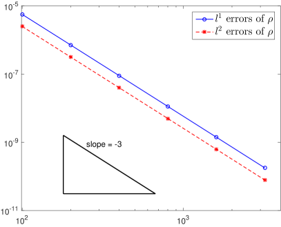
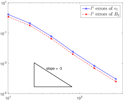
Figure 5.1: Numerical errors obtained by the PP third-order DG scheme at different mesh resolutions with $M^{d}$ cells. Left: the 1D smooth problem at $t=0.1$; right: the 2D smooth problem at $t=0.05$. The horizontal axis denotes the value of $M$.

Next, we simulate several MHD problems involving discontinuities. Before the PP limiting procedure, the WENO limiter [42] is also implemented with the aid of the local characteristic decomposition, to enhance the numerical stability of high-order DG schemes in resolving the strong discontinuities and their interactions. The 2D WENO limiter is combined with the locally divergence-free reconstruction approach in [66]. The WENO limiter is only employed adaptively in the “trouble” cells detected by the indicator of [33].

5.2 Riemann problems

Two 1D Riemann problems are solved. The first is a 1D vacuum shock tube problem (cf. [16]) with the initial data

$$(\rho,{\bf v},p,{\bf B})(x,0)=\begin{cases}(10^{-12},~{}0,~{}0,~{}0,~{}10^{-12},~{}0,~{}0,~{}0),\quad&x<0,\\ (1,~{}0,~{}0,~{}0,~{}0.5,~{}0,~{}1,~{}0),\quad&x>0.\end{cases}$$

It is used to demonstrate that our 1D PP DG scheme can handle extremely low density and pressure. The adiabatic index $\gamma=\frac{5}{3}$, and the computational domain is set as $[-0.5,0.5]$. Fig. 5.2 shows the density and pressure of the numerical solution on, respectively, the mesh of $200$ cells as well as those of a highly resolved solution with $5000$ cells at time $t=0.1$. One can observe that the solutions of low resolution and high resolution are in quite good agreement. We confirm that the low pressure and the low density are both correctly captured by comparing with the results in [16]. The PP third-order DG code is very robust during the simulation. It is noticed that, if the PP limiter is not used to enforce the condition (3.7), the code breaks down within a few time steps due to unphysical solution.

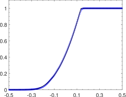
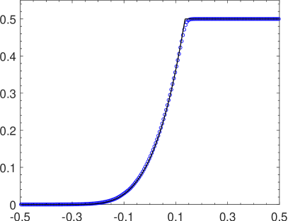
Figure 5.2: The density (left) and pressure (right) obtained by the PP third-order DG method on the meshes of $200$ cells (symbols “$\circ$”) and $5000$ cells (solid lines), respectively.

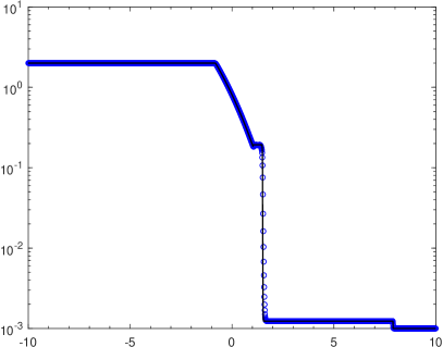
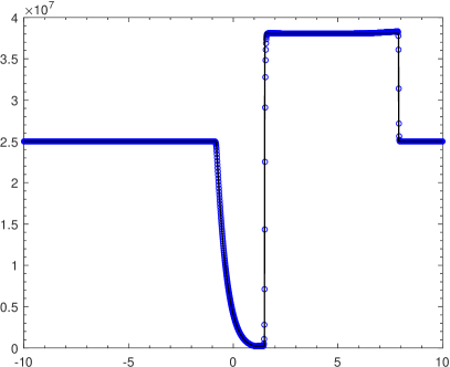
Figure 5.3: Numerical results at $t=0.00003$ obtained by the PP third-order DG method with $2000$ cells (symbols “$\circ$”) and $10000$ cells (solid lines). Left: log plot of density; right: magnetic pressure.

The second Riemann problem is a variant of the Leblanc problem (cf. [63]) of gas dynamics by adding a strong magnetic field. The initial condition is

$$(\rho,{\bf v},p,{\bf B})(x,0)=\begin{cases}(2,~{}0,~{}0,~{}0,~{}10^{9},~{}0,~{}5000,~{}5000),\quad&x<0,\\ (0.001,~{}0,~{}0,~{}0,~{}1,~{}0,~{}5000,~{}5000),\quad&x>0.\end{cases}$$

The initial pressure has a very large jump, and the plasma-beta at the right state is extremely low ($\beta=4\times 10^{-8}$), making the successful simulation of this problem a challenge. The computational domain is taken as $[-10,10]$. To fully resolve the wave structure of such a problem, a fine mesh is often required [63]. Fig. 5.3 displays the numerical results at $t=0.00003$ obtained by the PP third-order DG scheme with $2000$ cells and $10000$ cells, respectively. It is observed that the strong discontinuities are well resolved, and the low resolution and high resolution are highly in agreement. Fig. 5.4 gives a comparison of the numerical solutions resolved by using the proposed HLL flux and the global LF flux of [51], respectively. As expected, the PP DG method with the HLL flux exhibits better resolution. In this extreme test, it is also necessary to enforce the condition (3.7) by the PP limiting procedure, otherwise negative pressure will appear in the cell averages of the DG solution.

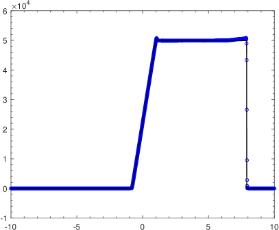
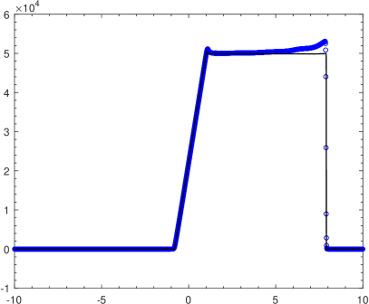
Figure 5.4: Same as Fig. 5.3 except for the velocity $v_{1}$ obtained by using the proposed HLL flux (left) and the global LF flux (right).

5.3 Blast problem

This test was first introduced by Balsara and Spicer [8], and has become a benchmark for testing 2D MHD codes. If the low gas pressure, strong magnetic field or small plasma-beta is involved, then simulating such MHD blast problems can be very challenging. Therefore, it is often used to examine the robustness of MHD schemes; see e.g., [13, 16].

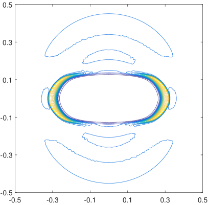
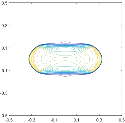
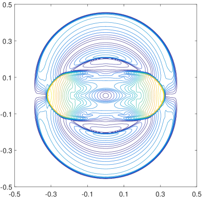
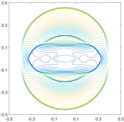
Figure 5.5: The contour plots of density (top left), pressure (top right), velocity $|{\bf v}|$ (bottom left) and magnetic pressure (bottom right) at time $t=0.01$ for the blast problem.

The simulation is implemented in $[-0.5,0.5]^{2}$ with outflow boundary conditions. Our setup is the same as in [8, 13]. Initially, the domain is filled with fluid at rest with unit density. The explosion zone $(r<0.1)$ has a pressure of $1000$, while the ambient medium $(r>0.1)$ has a pressure of $0.1$, where $r=\sqrt{x^{2}+y^{2}}$. The magnetic field is initialized in the $x$-direction as $100/\sqrt{4\pi}$. For this setup, the ambient medium has a small plasma-beta (about $2.51\times 10^{-4}$). Our numerical results at $t=0.01$, obtained by the PP third-order DG method with $320\times 320$ cells, are displayed in Fig. 5.5. Our results agree well with those in [8, 35, 16], and the density profile is well resolved with much less oscillations than those shown in [8, 16]. The velocity profile clearly shows higher resolution than that in [52] obtained by the same DG method but with the global LF flux. We also notice that, if the PP limiter is turned off, the condition (4.13) will be violated since $t\approx 2.24\times 10^{-4}$, and the method will fail due to negative numerical pressure.

5.4 Shock cloud interaction

This test [18] simulates the disruption of a high density cloud by a strong shock wave, and has been widely simulated in the literature (e.g., [46, 2]). We employ the same setup as in [46, 2]. The simulation is implemented in the domain $\Omega=[0,1]^{2}$ with the right boundary specified as supersonic inflow condition and the others as outflow conditions. The adiabatic index $\gamma=\frac{5}{3}$, and the initial conditions are given by the two states

$$(\rho,{\bf v},p,{\bf B})=\begin{cases}(3.86859,0,0,0,167.345,0,2.1826182,-2.1826182),\quad&x<0.6,\\ (1,-11.2536,0,0,1,0,0.56418958,0.56418958),\quad&x>0.6,\end{cases}$$

separated by a discontinuity parallel to the $y$-axis at $x=0.6$. To the right of the discontinuity there is a circular cloud of radius $0.15$, centered at $x=0.8$ and $y=0.5$. The cloud has the same states as the surrounding fluid except for a higher density of $10$.

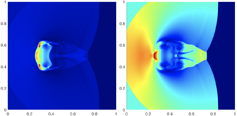
Figure 5.6: The schlieren images of density (left) and pressure (right) at time $t=0.06$ for the shock cloud interaction problem.

We simulate this problem by using our PP third-order DG method with $400\times 400$ cells. The numerical results at time $t=0.06$ are shown in Fig. 5.6. It is seen that the complex flow structures and interactions are correctly captured, and the results agree well with those in, for example, [46, 2]. In this test, it is also necessary to employ the PP limiter to enforce the condition (4.13). We also observe that, if the penalty term is dropped from our PP DG method, negative pressure will appear in the cell average of the DG solutions and the code breaks down at $t\approx 0.014$, because the resulting scheme (namely the locally divergence-free DG method with the proposed HLL flux and the PP and WENO limiters) is not PP in general. This further confirms the importance of the penalty term.

5.5 Astrophysical jets

The last test is to simulate jet flow, which is relevant in astrophysics. In a high Mach number jet with strong magnetic field, the internal energy is very small compared to the huge magnetic and/or kinetic energies, thus negative pressure is very likely to be produced in the numerical simulations. Moreover, there may exist shear flows, strong shock waves, and interface instabilities in high-speed jet flows. Successfully simulating such jet flows is indeed a challenge, cf. [63, 5, 53, 55].

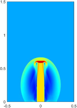
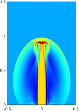
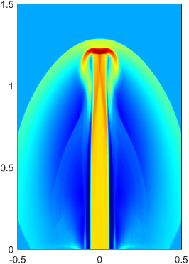
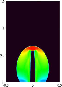
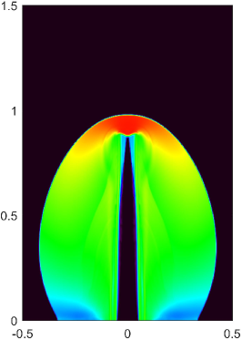
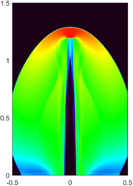
Figure 5.7: The schlieren images of density logarithm (top) and gas pressure logarithm (bottom) for the Mach 800 jet problem with $B_{a}=\sqrt{2000}$. From left to right: $t=0.001$, $0.0015$ and $0.002$.

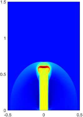
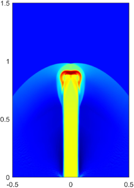
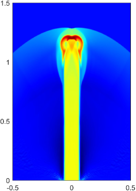
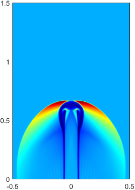
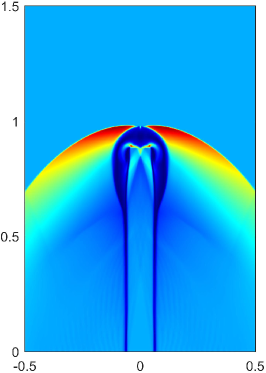
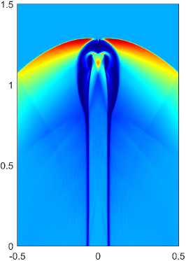
Figure 5.8: The schlieren images of density logarithm (top) and magnetic pressure (bottom) for the Mach 800 jet problem with $B_{a}=\sqrt{20000}$. From left to right: $t=0.001$, $0.0015$ and $0.002$.

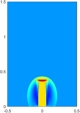
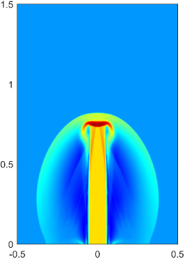
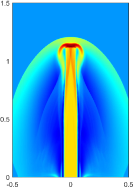
Figure 5.9: The schlieren images of density logarithm for the Mach 2000 jet problem with $B_{a}=\sqrt{20000}$. From left to right: $t=0.00025$, $0.0005$ and $0.00075$.

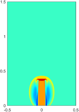
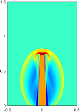
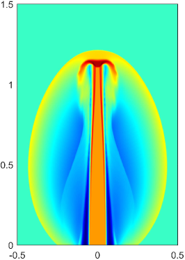
Figure 5.10: The schlieren images of density logarithm for the Mach 10000 jet problem with $B_{a}=\sqrt{20000}$. From left to right: $t=0.00005$, $0.0001$ and $0.00015$.

We consider the Mach 800 MHD jets proposed in [51, 52] and extended from the gas dynamical jet of Balsara [5] by adding a magnetic field. Initially, the domain $[-0.5,0.5]\times[0,1.5]$ is full of the static ambient medium with $(\rho,p)=(0.1\gamma,1)$. The adiabatic index $\gamma=1.4$. A Mach 800 dense jet is injected in the $y$-direction through the inlet part ($\left|x\right|<0.05$) on the bottom boundary ($y=0$). The fixed inflow condition with $(\rho,p,v_{1},v_{2},v_{3})=(\gamma,1,0,800,0)$ is specified on the nozzle $\{y=0,\left|x\right|<0.05\}$, while the other boundary conditions are outflow. A magnetic field $(0,B_{a},0)$ is initialized along the $y$-direction. As $B_{a}$ is set larger, this test becomes more challenging. We set computational domain as $[0,0.5]\times[0,1.5]$ with the reflecting boundary condition specified at $x=0$, and divided it into $200\times 600$ cells. We here show our numerical results in two strongly magnetized cases: (i) $B_{a}=\sqrt{2000}$, and the corresponding plasma-beta $\beta_{a}=10^{-3}$; (ii) $B_{a}=\sqrt{20000}$, and the corresponding plasma-beta $\beta_{a}=10^{-4}$. The schlieren images of the numerical solutions for these two cases are respectively displayed in Figs. 5.7 and 5.8 within the domain $[-0.5,0.5]\times[0,1.5]$. Those plots clearly show the time evolution of the jets. It is seen that the flow structures in different magnetized cases are very different. The present method well captures the Mach shock wave at the jet head and other discontinuities with high resolution. The results agree with those in [52] computed by the PP DG method with a global LF flux. In these extreme tests, our PP method exhibits good robustness without using any artificial treatment. We also perform the tests with varied Mach numbers, and the method also works very robustly. For example, the numerical result for a Mach 2000 jet with $B_{a}=\sqrt{20000}$ is displayed in Fig. 5.9. Interestingly, the flow structures are similar to those in Fig. 5.7 of the Mach 800 jet with a weaker magnetic field $B_{a}=\sqrt{2000}$. This is probably due to the huge kinetic energy, which becomes dominant and weakens the effect of magnetic field. The dynamics of the Mach 2000 jet evolve much faster than the Mach 800 jet, as expected. A higher Mach (Mach 10000) jet with $B_{a}=\sqrt{20000}$ is further simulated and shown in Fig. 5.10. We see that this jet shape is thinner.

In the above simulations, it is necessary to employ the PP limiting procedure to meet the condition (4.13), which is not satisfied automatically. To confirm the importance of the proposed penalty term in our PP schemes, we have also performed the above tests by dropping the penalty term and keeping the PP and WENO limiters turned on. The resulting scheme is actually the locally divergence-free, conservative, third-order DG method with PP and WENO limiters. We find that this scheme with either the proposed HLL flux or the global LF flux, which is generally not PP in theory, cannot run the above jet tests. The failure results from negative numerical pressure produced in the cell averages of the DG solution. We observe that, without the proposed penalty term, the code also fails on a refined mesh, and also for more strongly magnetized cases. This, again, demonstrates that the proposed penalty term is really crucial for guaranteeing the PP property.

6 Conclusions

In this paper, we proposed and analyzed provably PP high-order DG and finite volume schemes for the ideal MHD on general meshes. The unified auxiliary theories were built for rigorous PP analysis of numerical schemes with HLL-type flux on an arbitrary polytopal mesh. A close relation was established between the PP property and the discrete divergence of magnetic field on general meshes. We also derived explicit estimates of the wave speeds in the HLL flux to ensure the provably PP property. In the 1D case, we proved that the standard finite volume and DG methods with the proposed HLL flux are PP, under a condition accessible by a PP limiter. In the multidimensional cases, we constructed provably PP high-order DG schemes based on suitable discretization of the modified MHD system (1.4). In addition to the proper wave speeds in the numerical flux and a standard PP limiter, we demonstrated that a coupling of two divergence-controlling techniques is also crucial for achieving the provably PP property. The two techniques are the locally divergence-free DG element and a properly discretized Godunov–Powell source term, which control the divergence error within each cell and across the cell interfaces, respectively. Our analysis clearly revealed that these two techniques exactly contribute the discrete divergence terms which are absent in a standard multidimensional DG schemes but very important for ensuring the PP property. We also proved in Appendix A the positivity of the strong solution of the modified MHD system (1.1). Such a feature, not enjoyed by the conservative system (1.1) (see [52]), can serve as a justification for designing provably PP multidimensional schemes based on the modified system (1.4). The analysis and findings in this paper provide a clear understanding, at both discrete and continuous levels, of the relation between the PP property and the divergence-free constraint. The proposed framework and analysis techniques as well as the provenly PP schemes can also be useful for investigating or designing other PP schemes for the ideal MHD.

Several numerical tests were conducted on 1D mesh and 2D rectangular mesh, to confirm the provenly PP property and to demonstrate the effectiveness of the proposed PP techniques. The implementation of our PP DG schemes on unstructured triangular meshes is ongoing and will be reported separately in the future.

Appendix A Positivity of strong solutions of the modified MHD system

In [52], we analytically demonstrated that the exact smooth solution of the conservative MHD system (1.1) may fail to be PP if the divergence-free condition (1.2) is violated. Here we would like to show that the strong solutions of the modified MHD system (1.4) always retain the positivity of density and pressure even if the divergence-free condition (1.2) is not satisfied. It is reasonable to hope that such a claim may also hold for the weak entropy solutions of (1.4).

Consider the initial-value problem of the system (1.4), for ${\bf x}\in{\mathbb{R}}^{d}$ and $t>0$, with initial data

$$(\rho,{\bf v},p,{\bf B})({\bf x},0)=(\rho_{0},{\bf v}_{0},p_{0},{\bf B}_{0})({\bf x}),$$ (A.1)

and the ideal EOS $p=(\gamma-1)\rho e$, where $\gamma>1$. Using the method of characteristics, one can show the following result.

Proposition A.1.

Assume that the initial data (A.1) are in $C^{1}({\mathbb{R}}^{d})$ with $\rho_{0}({\bf x})>0$ and $p_{0}({\bf x})>0,$ $\forall{\bf x}\in{\mathbb{R}}^{d}$. If the initial-value problem of (1.4) with (A.1) has a $C^{1}$ solution $(\rho,{\bf v},p,{\bf B})({\bf x},t)$ for ${\bf x}\in{\mathbb{R}}^{d}$ and $0\leq t<T$, then the solution satisfies $\rho({\bf x},t)>0$ and $p({\bf x},t)>0$ for all ${\bf x}\in{\mathbb{R}}^{d}$ and $0\leq t<T$.

Proof.

Let $\frac{D}{Dt}:=\partial_{t}+{\bf v}({\bf x},t)\nabla\cdot$ be the directional derivative along the direction

$$\frac{d{\bf x}}{dt}={\bf v}({\bf x},t).$$ (A.2)

For any $\left(\bar{\bf x},\bar{t}\right)\in\mathbb{R}^{d}\times\mathbb{R}_{+}$, let ${\bf x}={\bf x}(t;\bar{\bf x},\bar{t})$ be the integral curve of (A.2) through the point $\left(\bar{\bf x},\bar{t}\right)$. Denote ${\bf x}_{0}(\bar{\bf x},\bar{t}):={\bf x}(0;\bar{\bf x},\bar{t})$, then, at $t=0$, the curve passes through the point $\left({\bf x}_{0}(\bar{\bf x},\bar{t}),0\right)$. Recall that, for smooth solutions, the first equation of the system (1.4) can be reformulated as

$$\frac{D\rho}{Dt}=-\rho\nabla\cdot{\bf v}.$$ (A.3)

Integrating Eq. (A.3) along the curve ${\bf x}={\bf x}(t;\bar{\bf x},\bar{t})$ gives

$$\rho(\bar{\bf x},\bar{t})=\rho_{0}({\bf x}_{0}(\bar{\bf x},\bar{t}))\exp\left(-\int_{0}^{\bar{t}}\nabla\cdot{\bf v}({\bf x}(t;\bar{\bf x},\bar{t}),t)dt\right)>0.$$

For smooth solutions, we derive from the modified system (1.4) the pressure equation

$$\frac{Dp}{Dt}=-\gamma p\nabla\cdot{\bf v},$$ (A.4)

which implies $p(\bar{\bf x},\bar{t})=p_{0}({\bf x}_{0}(\bar{\bf x},\bar{t}))\exp\left(-\gamma\int_{0}^{\bar{t}}\nabla\cdot{\bf v}({\bf x}(t;\bar{\bf x},\bar{t}),t)dt\right)>0.$ $\blacksquare$

Remark A.1.

By similar arguments one can show that the above proposition also holds for the modified MHD equations introduced by Janhunen [32], because the corresponding equations for density and pressure are exactly also (A.3) and (A.4), respectively. This may explain why it is also possible to develop PP schemes based on proper discretization of Janhunen’s MHD system, cf. [32, 10, 48, 49].

Recall that the pressure equation associated with the conservative system (1.1) is

$$\frac{Dp}{Dt}=-\gamma p\nabla\cdot{\bf v}-(\gamma-1)({\bf v}\cdot{\bf B})\nabla\cdot{\bf B},$$

which, in comparison with (A.4), has an additional term proportional to $\nabla\cdot{\bf B}$. As shown in [52], due to this term, negative pressure can appear in the exact smooth solution of the conservative MHD system (1.1) if $\nabla\cdot{\bf B}\neq 0$.

Appendix B Review of the positivity-preserving limiter

We employ a simple PP limiter to enforce the condition (3.7) or (4.13) for our 1D or 2D PP schemes. The limiter was originally proposed by Zhang and Shu [62, 63, 64] for scalar conservation laws and the compressible Euler equations. It was extended to the ideal MHD case in [13]. For readers’ convenience, we here briefly review this limiter. It is worth noting that the PP limiter works only when the cell averages of the numerical solutions always stay in ${\mathcal{G}}$. This is rigorously proved for our PP high-order schemes, but does not always hold for the standard multidimensional DG schemes without the proposed penalty term.

We perform the PP limiter separately for each cell. Let $K$ denote a cell, and ${\mathbb{S}}_{K}$ be the quadrature points involved in the condition (3.7) or (4.13) in $K$. Let ${\bf U}_{K}^{n}({\bf x})$ be the approximate polynomial solution within $K$, and $\bar{\bf U}_{K}^{n}$ be the cell average which is always preserved in $\mathcal{G}$ by our PP schemes. If ${\bf U}_{K}^{n}({\bf x})\notin{\mathcal{G}}$ for some ${\bf x}\in{\mathbb{S}}_{K}$, then we seek the modified polynomial $\widetilde{\bf U}_{K}^{n}({\bf x})$ with the same cell average such that $\widetilde{\bf U}_{K}^{n}({\bf x})\in{\mathcal{G}}$ for all ${\bf x}\in{\mathbb{S}}_{K}$. To avoid the effect of the rounding error, we introduce two sufficiently small positive numbers, $\epsilon_{1}$ and $\epsilon_{2}$, as the desired lower bounds for density and internal energy, respectively, such that $\bar{\bf U}_{K}^{n}\in{\mathcal{G}}_{\epsilon}=\{{\bf U}:\rho\geq\epsilon_{1},{\mathcal{E}}({\bf U})\geq\epsilon_{2}\}$; e.g., take $\epsilon_{1}=\min\{10^{-13},\bar{\rho}_{K}^{n}\}$ and $\epsilon_{2}=\min\{10^{-13},{\mathcal{E}}(\bar{\bf U}_{K}^{n})\}$.

The PP limiting procedure consists of two steps. First, modify the density to enforce the positivity by

$$\widehat{\rho}_{K}({\bf x})=\theta_{1}(\rho_{K}^{n}({\bf x})-\bar{\rho}_{K}^{n})+\bar{\rho}_{K}^{n},\quad\theta_{1}=\min\left\{1,\frac{\bar{\rho}_{K}^{n}-\epsilon_{1}}{\bar{\rho}_{K}^{n}-\min_{{\bf x}\in{\mathbb{S}}_{K}}\rho_{K}^{n}({\bf x})}\right\}.$$

Then modify $\widehat{\bf U}_{K}({\bf x}):=(\widehat{\rho}_{K}({\bf x}),{\bf m}_{K}^{n}({\bf x}),{\bf B}_{K}^{n}({\bf x}),E_{K}^{n}({\bf x}))^{\top}$ to enforce the positivity of internal energy by

$$\widetilde{\bf U}_{K}^{n}({\bf x})=\theta_{2}(\widehat{\bf U}_{K}({\bf x})-\bar{\bf U}_{K}^{n})+\bar{\bf U}_{K}^{n},\quad\theta_{2}=\min\left\{1,\frac{{\mathcal{E}}(\bar{\bf U}_{K}^{n})-\epsilon_{2}}{{\mathcal{E}}(\bar{\bf U}_{K}^{n})-\min_{{\bf x}\in{\mathbb{S}}_{K}}{\mathcal{E}}\big{(}\widehat{\bf U}_{K}({\bf x})\big{)}}\right\}.$$

It is easy to verify that $\widetilde{\bf U}_{K}^{n}({\bf x})$ belongs to ${\mathcal{G}}_{\epsilon}$ for all ${\bf x}\in{\mathbb{S}}_{K}$ and has the cell average $\bar{\bf U}_{K}^{n}$. Such a limiter can also maintain the approximation accuracy; see [62, 63, 61].

References

- [1] R. Artebrant and M. Torrilhon, Increasing the accuracy in locally divergence-preserving finite volume schemes for MHD, J. Comput. Phys., 227 (2008), pp. 3405–3427.
- [2] J. Balbás and E. Tadmor, Nonoscillatory central schemes for one- and two-dimensional magnetohydrodynamics equations. II: High-order semidiscrete schemes, SIAM J. Sci. Comput., 28 (2006), pp. 533–560.
- [3] D. S. Balsara, Second-order-accurate schemes for magnetohydrodynamics with divergence-free reconstruction, Astrophys. J. Suppl. Ser., 151 (2004), pp. 149–184.
- [4] D. S. Balsara, Multidimensional HLLE Riemann solver: Application to Euler and magnetohydrodynamic flows, J. Comput. Phys., 229 (2010), pp. 1970–1993.
- [5] D. S. Balsara, Self-adjusting, positivity preserving high order schemes for hydrodynamics and magnetohydrodynamics, J. Comput. Phys., 231 (2012), pp. 7504–7517.
- [6] D. S. Balsara, M. Dumbser, and R. Abgrall, Multidimensional HLLC Riemann solver for unstructured meshes — With application to Euler and MHD flows, J. Comput. Phys., 261 (2014), pp. 172–208.
- [7] D. S. Balsara and D. Spicer, Maintaining pressure positivity in magnetohydrodynamic simulations, J. Comput. Phys., 148 (1999), pp. 133–148.
- [8] D. S. Balsara and D. Spicer, A staggered mesh algorithm using high order Godunov fluxes to ensure solenoidal magnetic fields in magnetohydrodynamic simulations, J. Comput. Phys., 149 (1999), pp. 270–292.
- [9] F. Bouchut, C. Klingenberg, and K. Waagan, A multiwave approximate Riemann solver for ideal MHD based on relaxation. I: theoretical framework, Numer. Math., 108 (2007), pp. 7–42.
- [10] F. Bouchut, C. Klingenberg, and K. Waagan, A multiwave approximate Riemann solver for ideal MHD based on relaxation II: numerical implementation with 3 and 5 waves, Numer. Math., 115 (2010), pp. 647–679.
- [11] J. U. Brackbill and D. C. Barnes, The effect of nonzero on the numerical solution of the magnetodydrodynamic equations, J. Comput. Phys., 35 (1980), pp. 426–430.
- [12] P. Chandrashekar and C. Klingenberg, Entropy stable finite volume scheme for ideal compressible MHD on 2-D Cartesian meshes, SIAM J. Numer. Anal., 54 (2016), pp. 1313–1340.
- [13] Y. Cheng, F. Li, J. Qiu, and L. Xu, Positivity-preserving DG and central DG methods for ideal MHD equations, J. Comput. Phys., 238 (2013), pp. 255–280.
- [14] A. J. Christlieb, X. Feng, D. C. Seal, and Q. Tang, A high-order positivity-preserving single-stage single-step method for the ideal magnetohydrodynamic equations, J. Comput. Phys., 316 (2016), pp. 218–242.
- [15] A. J. Christlieb, Y. Liu, Q. Tang, and Z. Xu, High order parametrized maximum-principle-preserving and positivity-preserving WENO schemes on unstructured meshes, J. Comput. Phys., 281 (2015), pp. 334–351.
- [16] A. J. Christlieb, Y. Liu, Q. Tang, and Z. Xu, Positivity-preserving finite difference weighted ENO schemes with constrained transport for ideal magnetohydrodynamic equations, SIAM J. Sci. Comput., 37 (2015), pp. A1825–A1845.
- [17] A. J. Christlieb, J. A. Rossmanith, and Q. Tang, Finite difference weighted essentially non-oscillatory schemes with constrained transport for ideal magnetohydrodynamics, J. Comput. Phys., 268 (2014), pp. 302–325.
- [18] W. Dai and P. R. Woodward, A simple finite difference scheme for multidimensional magnetohydrodynamical equations, J. Comput. Phys., 142 (1998), pp. 331–369.
- [19] S. F. Davis, Simplified second-order Godunov-type methods, SIAM J. Sci. Stat. Comp., 9 (1988), pp. 445–473.
- [20] A. Dedner, F. Kemm, D. Kröner, C.-D. Munz, T. Schnitzer, and M. Wesenberg, Hyperbolic divergence cleaning for the MHD equations, J. Comput. Phys., 175 (2002), pp. 645–673.
- [21] P. J. Dellar, A note on magnetic monopoles and the one-dimensional MHD Riemann problem, J. Comput. Phys., 172 (2001), pp. 392–398.
- [22] J. Du and C.-W. Shu, Positivity-preserving high-order schemes for conservation laws on arbitrarily distributed point clouds with a simple WENO limiter, Int. J. Numer. Anal. Model., 15 (2018), pp. 1–25.
- [23] B. Einfeldt, C.-D. Munz, P. L. Roe, and B. Sjögreen, On Godunov-type methods near low densities, J. Comput. Phys., 92 (1991), pp. 273–295.
- [24] C. R. Evans and J. F. Hawley, Simulation of magnetohydrodynamic flows: a constrained transport method, Astrophys. J., 332 (1988), pp. 659–677.
- [25] P. Fu, F. Li, and Y. Xu, Globally divergence-free discontinuous Galerkin methods for ideal magnetohydrodynamic equations, J. Sci. Comput., (2018).
- [26] F. G. Fuchs, A. D. McMurry, S. Mishra, N. H. Risebro, and K. Waagan, Approximate Riemann solvers and robust high-order finite volume schemes for multi-dimensional ideal MHD equations, Commun. Comput. Phys., 9 (2011), pp. 324–362.
- [27] T. A. Gardiner and J. M. Stone, An unsplit Godunov method for ideal MHD via constrained transport, J. Comput. Phys., 205 (2005), pp. 509–539.
- [28] S. K. Godunov, Symmetric form of the equations of magnetohydrodynamics, Numerical Methods for Mechanics of Continuum Medium, 1 (1972), pp. 26–34.
- [29] S. Gottlieb, D. I. Ketcheson, and C.-W. Shu, High order strong stability preserving time discretizations, J. Sci. Comput., 38 (2009), pp. 251–289.
- [30] K. Gurski, An HLLC-type approximate Riemann solver for ideal magnetohydrodynamics, SIAM J. Sci. Comput., 25 (2004), pp. 2165–2187.
- [31] X. Y. Hu, N. A. Adams, and C.-W. Shu, Positivity-preserving method for high-order conservative schemes solving compressible Euler equations, J. Comput. Phys., 242 (2013), pp. 169–180.
- [32] P. Janhunen, A positive conservative method for magnetohydrodynamics based on HLL and Roe methods, J. Comput. Phys., 160 (2000), pp. 649–661.
- [33] L. Krivodonova, J. Xin, J.-F. Remacle, N. Chevaugeon, and J. E. Flaherty, Shock detection and limiting with discontinuous Galerkin methods for hyperbolic conservation laws, Appl. Numer. Math., 48 (2004), pp. 323–338.
- [34] F. Li and C.-W. Shu, Locally divergence-free discontinuous Galerkin methods for MHD equations, J. Sci. Comput., 22 (2005), pp. 413–442.
- [35] F. Li, L. Xu, and S. Yakovlev, Central discontinuous Galerkin methods for ideal MHD equations with the exactly divergence-free magnetic field, J. Comput. Phys., 230 (2011), pp. 4828–4847.
- [36] S. Li, An HLLC Riemann solver for magneto-hydrodynamics, J. Comput. Phys., 203 (2005), pp. 344–357.
- [37] C. Liang and Z. Xu, Parametrized maximum principle preserving flux limiters for high order schemes solving multi-dimensional scalar hyperbolic conservation laws, J. Sci. Comput., 58 (2014), pp. 41–60.
- [38] Y. Liu, C.-W. Shu, and M. Zhang, Entropy stable high order discontinuous Galerkin methods for ideal compressible MHD on structured meshes, J. Comput. Phys., 354 (2018), pp. 163–178.
- [39] T. Miyoshi and K. Kusano, A multi-state HLL approximate Riemann solver for ideal magnetohydrodynamics, J. Computat. Phys., 208 (2005), pp. 315–344.
- [40] K. G. Powell, An approximate Riemann solver for magnetohydrodynamics (that works in more than one dimension), Tech. Report ICASE Report No. 94-24, NASA Langley, VA, 1994.
- [41] K. G. Powell, P. Roe, R. Myong, and T. Gombosi, An upwind scheme for magnetohydrodynamics, in 12th Computational Fluid Dynamics Conference, 1995, p. 1704.
- [42] J. Qiu and C.-W. Shu, Runge–Kutta discontinuous Galerkin method using WENO limiters, SIAM J. Sci. Comput., 26 (2005), pp. 907–929.
- [43] D. Ryu, F. Miniati, T. Jones, and A. Frank, A divergence-free upwind code for multidimensional magnetohydrodynamic flows, Astrophys. J., 509 (1998), pp. 244–255.
- [44] D. C. Seal, Q. Tang, Z. Xu, and A. J. Christlieb, An explicit high-order single-stage single-step positivity-preserving finite difference WENO method for the compressible Euler equations, J. Sci. Comput., 68 (2016), pp. 171–190.
- [45] M. Torrilhon, Locally divergence-preserving upwind finite volume schemes for magnetohydrodynamic equations, SIAM J. Sci. Comput., 26 (2005), pp. 1166–1191.
- [46] G. Tóth, The constraint in shock-capturing magnetohydrodynamics codes, J. Comput. Phys., 161 (2000), pp. 605–652.
- [47] F. Vilar, C.-W. Shu, and P.-H. Maire, Positivity-preserving cell-centered lagrangian schemes for multi-material compressible flows: From first-order to high-orders. Part II: the two-dimensional case, J. Comput. Phys., 312 (2016), pp. 416–442.
- [48] K. Waagan, A positive MUSCL-Hancock scheme for ideal magnetohydrodynamics, J. Comput. Phys., 228 (2009), pp. 8609–8626.
- [49] K. Waagan, C. Federrath, and C. Klingenberg, A robust numerical scheme for highly compressible magnetohydrodynamics: Nonlinear stability, implementation and tests, J. Comput. Phys., 230 (2011), pp. 3331–3351.
- [50] K. Wu, Design of provably physical-constraint-preserving methods for general relativistic hydrodynamics, Phys. Rev. D, 95 (2017), 103001.
- [51] K. Wu, Positivity-preserving analysis of numerical schemes for ideal magnetohydrodynamics, SIAM J. Numer. Anal., 56 (2018), pp. 2124–2147.
- [52] K. Wu and C.-W. Shu, Provably positive discontinuous Galerkin methods for multidimensional ideal magnetohydrodynamics, SIAM J. Sci. Comput., submitted (2018).
- [53] K. Wu and H. Tang, High-order accurate physical-constraints-preserving finite difference WENO schemes for special relativistic hydrodynamics, J. Comput. Phys., 298 (2015), pp. 539–564.
- [54] K. Wu and H. Tang, Admissible states and physical-constraints-preserving schemes for relativistic magnetohydrodynamic equations, Math. Models Methods Appl. Sci., 27 (2017), pp. 1871–1928.
- [55] K. Wu and H. Tang, Physical-constraint-preserving central discontinuous Galerkin methods for special relativistic hydrodynamics with a general equation of state, Astrophys. J. Suppl. Ser., 228 (2017), 3.
- [56] T. Xiong, J.-M. Qiu, and Z. Xu, Parametrized positivity preserving flux limiters for the high order finite difference WENO scheme solving compressible Euler equations, J. Sci. Comput., 67 (2016), pp. 1066–1088.
- [57] Z. Xu, Parametrized maximum principle preserving flux limiters for high order schemes solving hyperbolic conservation laws: one-dimensional scalar problem, Math. Comp., 83 (2014), pp. 2213–2238.
- [58] Z. Xu, D. S. Balsara, and H. Du, Divergence-free WENO reconstruction-based finite volume scheme for solving ideal MHD equations on triangular meshes, Commun. Comput. Phys., 19 (2016), pp. 841–880.
- [59] Z. Xu and X. Zhang, Bound-preserving high order schemes, in Handbook of Numerical Methods for Hyperbolic Problems: Applied and Modern Issues, edited by R. Abgrall and C.-W. Shu, vol. 18, North-Holland, Amsterdam, 2017, Elsevier.
- [60] S. Yakovlev, L. Xu, and F. Li, Locally divergence-free central discontinuous Galerkin methods for ideal MHD equations, J. Comput. Sci., 4 (2013), pp. 80–91.
- [61] X. Zhang, On positivity-preserving high order discontinuous Galerkin schemes for compressible Navier-Stokes equations, J. Comput. Phys., 328 (2017), pp. 301–343.
- [62] X. Zhang and C.-W. Shu, On maximum-principle-satisfying high order schemes for scalar conservation laws, J. Comput. Phys., 229 (2010), pp. 3091–3120.
- [63] X. Zhang and C.-W. Shu, On positivity-preserving high order discontinuous Galerkin schemes for compressible Euler equations on rectangular meshes, J. Comput. Phys., 229 (2010), pp. 8918–8934.
- [64] X. Zhang and C.-W. Shu, Positivity-preserving high order discontinuous Galerkin schemes for compressible Euler equations with source terms, J. Comput. Phys., 230 (2011), pp. 1238–1248.
- [65] X. Zhang, Y. Xia, and C.-W. Shu, Maximum-principle-satisfying and positivity-preserving high order discontinuous galerkin schemes for conservation laws on triangular meshes, Journal of Scientific Computing, 50 (2012), pp. 29–62.
- [66] J. Zhao and H. Tang, Runge-Kutta discontinuous Galerkin methods for the special relativistic magnetohydrodynamics, J. Comput. Phys., 343 (2017), pp. 33–72.