Feynman integrals, toric geometry and mirror symmetry

Abstract

This expository text is about using toric geometry and mirror symmetry for evaluating Feynman integrals. We show that the maximal cut of a Feynman integral is a GKZ hypergeometric series. We explain how this allows to determine the minimal differential operator acting on the Feynman integrals. We illustrate the method on sunset integrals in two dimensions at various loop orders. The graph polynomials of the multi-loop sunset Feynman graphs lead to reflexive polytopes containing the origin and the associated variety are ambient spaces for Calabi-Yau hypersurfaces. Therefore the sunset family is a natural home for mirror symmetry techniques. We review the evaluation of the two-loop sunset integral as an elliptic dilogarithm and as a trilogarithm. The equivalence between these two expressions is a consequence of 1) the local mirror symmetry for the non-compact Calabi-Yau three-fold obtained as the anti-canonical hypersurface of the del Pezzo surface of degree 6 defined by the sunset graph polynomial and 2) that the sunset Feynman integral is expressed in terms of the local Gromov-Witten prepotential of this del Pezzo surface.

1 Introduction

Scattering amplitudes are fundamental quantities used to understand fundamental interactions and the elementary constituents in Nature. It is well known that scattering amplitudes are used in particle physics to compare the theoretical predictions to experimental measurements in particle colliders (see Bendavid:2018nar for instance). More recently the use of modern developments in scattering amplitudes have been extended to gravitational physics like unitarity methods to gravitational wave physics Neill:2013wsa ; Bjerrum-Bohr:2013bxa ; Cachazo:2017jef ; Guevara:2017csg ; Bjerrum-Bohr:2018xdl .

The $l$-loop scattering amplitude $A_{n,l}^{D}(\underline{s},\underline{m}^{2})$ between $n$ fields in $D$ dimensions is a function of the kinematics invariants $\underline{s}=\{s_{ij}=(p_{i}+p_{j})^{2},1\leq i,j\leq n\}$ where $p_{i}$ are the incoming momenta of the external particle, and the internal masses $\underline{m}^{2}=(m_{1},\dots,m_{r})$.

We focus on the questions : what kind of function is a Feynman integral? What is the best analytic representation?

The answer to these questions depend very strongly on which properties one wants to display. An analytic representation suitable for an high precision numerical evaluation may not be the one that displays the mathematical nature of the integral.

For instance the two-loop sunset integral has received many different, but equivalent, analytical expressions: hypergeometric and Lauricella functions Tarasov:2006nk ; Bauberger:1994by , Bessel integral representation Bailey:2008ib ; Broadhurst:2008mx ; Broadhurst:2016myo , Elliptic integrals Caffo:1999nk ; Laporta:2004rb , Elliptic polylogarithms Adams:2014vja ; Adams:2015gva ; Adams:2015ydq ; Adams:2016vdo ; Adams:2018ulb ; Adams:2018yqc ; Bloch:2016izu and trilogarithms Bloch:2016izu .

The approach that we will follow here will be guided by the geometry of the graph polynomial using the parametric representation of the Feynman integral. In §2 we review the description of the Feynman integral $I_{\Gamma}$ for a graph $\Gamma$ in parametric space. We focus on the properties of the second Symanzik polynomial as a preparation for the toric approach used in §3. In §2.2 we show that the maximal cut $\pi_{\Gamma}$ of a Feynman integral has a parametric representation similar to the one of the Feynman integral $I_{\Gamma}$ where the only difference is the cycle of integration. The toric geometry approach is described in §3. In section 3.2 we explain that the maximal cut integral is an hypergeometric series from the Gel’fand-Kapranov-Zelevinski (GKZ) construction. In section 3.4, we show on examples how to derive the minimal differential operator annihilating the maximal cut integral. In §4 we review the evaluation of the two-loop sunset integral in two space-time dimensions. In section 4.1 we give its expression as an elliptic dilogarithm

$$I_{\circleddash}(p^{2},\xi_{1}^{2},\xi_{2}^{2},\xi_{3}^{2})\propto\varpi\,\sum_{i=1}^{6}c_{i}\sum_{n\geq 1}(\textrm{Li}_{2}(q^{n}z_{i})-(\textrm{Li}_{2}(-q^{n}z_{i}))$$ (1)

where $\varpi$ is a period of the elliptic curve defined by the graph polynomial, $q$ the nome function of the external momentum $p^{2}$ and internal masses $\xi_{i}^{2}$ for $i=1,2,3$. In §4.2 we show that the sunset integral evaluates as sum of trilogarithm functions in (231)

$$I_{\circleddash}(p^{2},\xi_{1}^{2},\xi_{2}^{2},\xi_{3}^{2})\propto\varpi\,(3(\log Q)^{3}\cr+\sum_{(n_{1},n_{2},n_{3})\geq 0}\left(d_{n_{1},n_{2},n_{3}}+\delta_{n_{1},n_{2},n_{3}}\log(-p^{2})\right)\textrm{Li}_{3}(\prod_{i=1}^{3}\xi_{i}^{2n_{i}}Q^{n_{i}})\,.$$ (2)

In §4.3 we show that the equivalence between theses two expression is the result of a local mirror map, $q\leftrightarrow Q$ in (237), for the non-compact Calabi-Yau three-fold obtained as the anti-canonical bundle over the del Pezzo 6 surface defined by the sunset graph polynomial. Remarkably the sunset Feynman integral is expressed in terms of the genus zero local Gromov-Witten prepotential Bloch:2016izu . Therefore this provides a natural application for Batyrev’s mirror symmetry techniques Batyrev94 . One remarkable fact is that the computation can be done using the existing technology of mirror symmetry developed in other physical Hosono:1993qy ; CKYZ ; Huang:2013yta or mathematics Doran:2011ti contexts.

2 Feynman integrals

A connected Feynman graph $\Gamma$ is determined by the number $n$ of propagators (internal edges), the number $l$ of loops, and the number $v$ of vertices. The Euler characteristic of the graph relates these three numbers as $v=n-l+1$, therefore only the number of loops $l$ and the number $n$ of propagators are needed.

In a momentum representation an $l$-loop with $n$ propagators Feynman graph reads

$$I_{\Gamma}(\underline{s},\underline{\xi}^{2},\underline{\nu},D):={(\mu^{2})^{\omega}\over\pi^{lD\over 2}}\,{\prod_{i=1}^{n}\Gamma(\nu_{i})\over\Gamma(\omega)}\,\int_{({\mathbb{R}}^{1,D-1})^{l}}\,{\prod_{i=1}^{l}d^{D}\ell_{i}\over\prod_{i=1}^{n}(q_{i}^{2}-m_{i}^{2}+i\varepsilon)^{\nu_{i}}}\,,$$ (3)

where $D$ is the space-time dimension, and we set $\omega:=\sum_{i=1}^{n}\nu_{i}-lD/2$ and $q_{i}$ is the momentum flowing in between the vertices $i$ and $i+1$. With $\mu^{2}$ a scale of dimension mass squared. From now we set $m_{i}^{2}=\xi_{i}^{2}\mu^{2}$ and $p_{i}\to p_{i}\mu$, with these new variables the $\mu^{2}$ dependence disappear. The internal masses are positive $\xi_{i}^{2}\geq 0$ with $1\leq i\leq n$. Finally $+i\varepsilon$ with $\varepsilon>0$ is the Feynman prescription for the propagators for a space-time metric of signature $(+-\cdots-)$. The arguments of the Feynman integral are $\underline{\xi}^{2}:=\{\xi_{1}^{2},\dots,\xi_{n}^{2}\}$ and $\nu:=\{\nu_{1},\dots,\nu_{n}\}$ and $\underline{s}:=\{s_{ij}=(p_{i}+p_{j})^{2}\}$ with $p_{i}$ with $i=1,\dots,v_{e}$ with $0\leq v_{e}\leq v$ the external momenta subject to the momentum conservation condition $p_{1}+\cdots+p_{v_{e}}=0$. There are $n$ internal masses $\xi_{i}^{2}$ with $1\leq i\leq n$, is $v_{e}$ is the number of external momenta we have $v_{e}$ external masses $p_{i}^{2}$ with $1\leq i\leq v_{e}$ (some of the mass could vanish but we do a generic counting here), and ${v_{e}(v_{e}-3)\over 2}$ independent kinematics invariants $s_{ij}=(p_{i}+p_{j})^{2}$. The total number of kinematic parameters is

$$N_{\Gamma}(n,l)=n+{v_{e}(v_{e}-1)\over 2}\leq N_{\Gamma}(n,l)^{max}=n+{(n-l+1)(n-l)\over 2}\,.$$ (4)

We set

$$I_{\Gamma}(\underline{s},\underline{m},D):=I_{\Gamma}(\underline{s},\underline{m},1,\dots,1,D)\,,$$ (5)

and for $\nu_{i}$ positive integers we have

$$I_{\Gamma}(\underline{s},\underline{m},\underline{\nu},D)=\prod_{i=1}^{n}\left({\partial\over\partial(\xi_{i}^{2})}\right)^{\nu_{i}}I_{\Gamma}(\underline{s},\underline{m},D)\,.$$ (6)

2.1 The parametric representation

Introducing the variables $x_{i}$ with $1\leq i\leq n$ such that

$$\sum_{i=1}^{n}x_{i}(q_{i}^{2}-\xi_{i}^{2})=(\ell^{\mu}_{1},\dots,\ell^{\mu}_{l})\cdot\Omega\cdot(\ell^{\mu}_{1},\dots,\ell^{\mu}_{l})^{T}\!+(\ell^{\mu}_{1},\dots,\ell^{\mu}_{l})\cdot(Q_{1}^{\mu},\dots,Q_{l}^{\mu})-J,$$ (7)

and performing standard Gaussian integrals on the $x_{i}$ (see Vanhove:2014wqa for instance) one obtains the equivalent parametric representation that we will use in these notes

$$I_{\Gamma}(\underline{s},\underline{\xi},\underline{\nu},D)=\int_{\Delta_{n}}\Omega_{\Gamma},$$ (8)

the integrand is the $n-1$-form

$$\Omega_{\Gamma}=\prod_{i=1}^{n}x_{i}^{\nu_{i}-1}\,{\mathcal{U}^{\omega-{D\over 2}}\over\mathcal{F}^{\omega}}\,\Omega_{0},$$ (9)

where $\Omega_{0}$ is the differential $n-1$-form on the real projective space $\mathbb{P}^{n-1}$

$$\Omega_{0}:=\sum_{j=1}^{n}(-1)^{j-1}\,x_{j}\,dx_{1}\wedge\cdots\wedge\widehat{dx_{j}}\wedge\cdots\wedge dx_{n}\,,$$ (10)

where $\widehat{dx_{j}}$ means that $dx_{j}$ is omitting in this sum. The domain of integration $\Delta_{n}$ is defined as

$$\Delta_{n}:=\{[x_{1},\cdots,x_{n}]\in\mathbb{P}^{n-1}|x_{i}\in\mathbb{R},x_{i}\geq 0\}.$$ (11)

The second Symanzik polynomial $\mathcal{F}=\mathcal{U}\,\bigl{(}(Q_{1}^{\mu},\dots,Q_{l}^{\mu})\cdot\Omega^{-1}\cdot(Q_{1}^{\mu},\dots,Q_{l}^{\mu})^{T}\\ -J\bigr{)}$, takes the form

$$\mathcal{F}(\underline{s},\underline{\xi}^{2},x_{1},\dots,x_{n})=\mathcal{U}(x_{1},\dots,x_{n})\,\left(\sum_{i=1}^{n}\xi_{i}^{2}x_{i}\right)-\sum_{1\leq i\leq j\leq n}s_{ij}\mathcal{G}_{ij}(x_{1},\dots,x_{n})$$ (12)

where the first Symanzik polynomial $\mathcal{U}(x_{1},\dots,x_{n})=\det\Omega$ and $\mathcal{G}_{ij}(x_{1},\dots,x_{n})$ are polynomial in the $x_{i}$ variables only.

• The first Symanzik polynomial $\mathcal{U}(x_{1},\dots,x_{n})$ is an homogeneous polynomial of degree $l$ in the Feynman parameters $x_{i}$ and it is at most linear in each of the $x_{i}$ variables. It does not depend on the physical parameters. This polynomial is also known as the Kirchhoff polynomial of graph $\Gamma$. Which is as well the determinant of the Laplacian of the graph see (Bogner:2010kv, , eq (35)) for a definition.

• The polynomial $\mathcal{U}(x_{1},\dots,x_{n})$ can be seen as the determinant of the period matrix $\Omega$ of the punctured Feynman graph Vanhove:2014wqa , i.e. the graph with amputated external legs. Or equivalently it can be obtained by considering the degeneration limit of a genus $l$ Riemann surfaces with $n$ punctures. This connection plays an important in understanding the quantum field theory Feynman integrals as the $\alpha^{\prime}\to 0$ limit of the corresponding string theory integrals Tourkine:2013rda ; Amini:2015czm .

• The graph polynomial $\mathcal{F}$ is homogeneous of degree $l+1$ in the variables $(x_{1},\dots,x_{n})$. This polynomial depends on the internal masses $\xi_{i}^{2}$ and the kinematic invariants $s_{ij}=(p_{i}\cdot p_{j})/\mu^{2}$. The polynomials $\mathcal{G}_{ij}$ are at most linear in all the variables $x_{i}$ since this is given by the spanning 2-trees Bogner:2010kv . Therefore if all internal masses are vanishing then $\mathcal{F}$ is linear in the Feynman parameters $x_{i}$.

• The $\mathcal{U}$ and $\mathcal{F}$ are independent of the dimension of space-time. The space-time dimension enters only in the powers of $\mathcal{U}$ and $\mathcal{F}$ in the parametric representation for the Feynman graphs. Therefore one can see the Feynman integral as a meromorphic function of $(\underline{\nu},D)$ in $\mathbb{C}^{1+n}$ as discussed in Speer .

• All the physical parameters, the internal masses $\xi_{i}^{2}$ and the kinematic variables $s_{ij}=(p_{i}\cdot p_{j})/\mu^{2}$ (that includes the external masses) enter linearly. This will be important for the toric approach described in §3.

2.2 Maximal cut

We show that the maximal cut of a Feynman graph has a nice parametric representation. Let us consider the maximal cut

$$\pi_{\Gamma}(\underline{s},\underline{\xi}^{2},D):={1\over\Gamma(\omega)(2i\pi)^{n}\pi^{lD\over 2}}\,\int_{({\mathbb{R}}^{1,D-1})^{L}}\,\prod_{i=1}^{l}d^{D}\ell_{i}\prod_{i=1}^{n}\delta(q_{i}^{2}-m_{i}^{2}+i\varepsilon),$$ (13)

of the Feynman integral $I_{\Gamma}(\underline{s},\underline{\xi}^{2},D)$ which is obtained from the Feynman integral in (3) by replacing all propagators by a delta-function

$${1\over d^{2}}={1\over 2i\pi}\delta(d^{2}).$$ (14)

Using the representation of the $\delta$-function

$$\delta(x)=\int_{-\infty}^{+\infty}dwe^{iwx},$$ (15)

we obtain that the integral is

$$\pi_{\Gamma}(\underline{s},\underline{m},D):={1\over\Gamma(\omega)(2i\pi)^{n}\pi^{lD\over 2}}\,\int_{{\mathbb{R}}^{(1,D-1)L}}e^{-i\sum_{i=1}^{n}x_{i}(\ell_{i}^{2}+m_{i}^{2}-i\varepsilon)}\prod_{i=1}^{l}d^{D}\ell_{i}\prod_{i=1}^{n}dx_{i}\,.$$ (16)

At this stage the integral is similar to the one leading to the parametric representation with the replacement $x_{r}\to ix_{r}$ with $x_{r}\in\mathbb{R}$. Setting $\tilde{x}_{r}=ix_{r}$ and performing the Gaussian integrals over the loop momenta, we get

$$\pi_{n}(\underline{s},\underline{\xi}^{2},D):={1\over(2i\pi)^{n}}\,\int_{i{\mathbb{R}}^{n}}{\widetilde{\mathcal{U}}^{\omega-{D\over 2}}\over\widetilde{\mathcal{F}}^{\omega}}\prod_{i=1}^{n}\delta(1-\sum_{i=1}^{n}\tilde{x}_{i})d\tilde{x}_{i}\,.$$ (17)

using the projective nature of the integrand we have ${\widetilde{\mathcal{U}}^{\omega-D/2}\over\widetilde{\mathcal{F}}^{\omega}}=i^{-n}{\mathcal{U}^{\omega-D/2}\over\mathcal{F}^{\omega}}$ and the integral can be rewritten as the torus integral

$$\pi_{\Gamma}(\underline{s},\underline{\xi}^{2},D):={1\over(2i\pi)^{n}}\,\int_{|x_{1}]=\cdots=|x_{n-1}|=1}{\mathcal{U}^{\omega-D/2}\over\mathcal{F}^{\omega}}\prod_{i=1}^{n-1}dx_{i}\,.$$ (18)

This integral shares the same integrand with the Feynman integral $I_{\Gamma}$ in (8) but the cycle of integration differs since we are integrating over a $n$-torus. We show in §3.2 that this maximal cut arises naturally from the toric formalism.

2.3 The differential equations

In general a Feynman integral $I_{\Gamma}(\underline{s},\underline{\xi}^{2},\underline{\nu},D)$ satisfies an inhomogeneous system of differential equations

$$\mathcal{L}_{\Gamma}I_{\Gamma}=\mathcal{S}_{\Gamma},$$ (19)

where the inhomogeneous term $\mathcal{S}_{\Gamma}$ essentially arises from boundary terms corresponding to reduced graph topologies where internal edges have been contracted. Knowing the maximal cut integral allows to determine differential operators $\mathcal{L}_{\Gamma}$

$$\mathcal{L}_{\Gamma}\pi_{\Gamma}(\underline{s},\underline{\xi}^{2},D)=0,$$ (20)

This fact has been exploited in Primo:2016ebd ; Primo:2017ipr ; Bosma:2017ens ; Frellesvig:2017aai to obtain the minimal order differential operator. The important remark in this construction is to use that the only difference between the Feynman integral $I_{\Gamma}$ and the maximal cut $\pi_{\Gamma}$ is the choice of cycle of integration. Since the Picard-Fuchs operator $\mathcal{L}_{\Gamma}$ acts as

$$\mathcal{L}_{\Gamma}\pi_{\Gamma}(\underline{s},\underline{\xi}^{2},D)=\int_{\gamma_{n}}\mathcal{L}_{\Gamma}\Omega_{F}=\int_{\gamma_{n}}d(\beta_{\Gamma})=0$$ (21)

this integral vanishes because the cycle $\gamma_{n}=\{|x_{1}|=\cdots=|x_{n}|=1\}$ has no boundaries $\partial\gamma_{n}=\emptyset$. In the case of the Feynman integral $I_{\Gamma}$ this is not longer true as

$$\mathcal{L}_{\Gamma}I_{\Gamma}(\underline{s},\underline{\xi}^{2},D)=\int_{\Delta_{n}}d(\beta_{\Gamma})=\int_{\partial\Delta_{n}}\beta_{\Gamma}=\mathcal{S}_{\Gamma}\neq 0\,.$$ (22)

The boundary contributions arises from the configuration with some of the Schwinger coordinate $x_{i}=0$ vanishing which corresponds to the so-called reduced topologies that are known to arises when applying the integration-by-part algorithm (see Chetyrkin:1981qh ; Tarasov:1997kx ; Tarasov:2017yyd for instance).

We illustrate this logic on some elementary examples of differential equations for multi-valued integrals relevant for the one- and two-loop massive sunset integrals discussed in this text.

The logarithmic integral

We consider the integral

$$I_{1}(t)=\int_{a}^{b}{dx\over x(x-t)}\,,$$ (23)

and its cut integral

$$\pi(t)=\int_{\gamma}{dx\over x(x-t)}\,,$$ (24)

where $\gamma$ is a cycle around the point $x=t$. Clearly we have

$${d\over dx}\left(1\over t-x\right)={1\over x(x-t)}+t{d\over dt}\left(1\over x(x-t)\right)\,,$$ (25)

therefore the integral $\pi(t)$ satisfies the differential equation

$$t{d\over dt}\pi(t)+\pi(t)=\int_{\gamma}{d\over dx}\left(1\over t-x\right)=0\,,$$ (26)

and the integral $I_{1}(t)$ satisfies

$$t{d\over dt}I_{1}(t)+I_{1}(t)=\int_{a}^{b}{d\over dx}\left(1\over t-x\right)={1\over b(b-t)}-{1\over a(a-t)}\,.$$ (27)

Changing variables from $t$ to $p^{2}$ or an internal mass will give the familiar differential equation for the one-loop bubble that will be commented further in §3.4.

Elliptic curve

The second example is the differential equation for the period of an elliptic curve $\mathcal{E}:y^{2}z=x(x-z)(x-tz)$ which is the geometry of the two-loop sunset integral. Consider the differential of the first kind on the elliptic curve

$$\omega={dx\over\sqrt{x(x-1)(x-t)}}\,,$$ (28)

this form can be seen as a residue evaluated on the elliptic curve $\omega=\textrm{Res}_{\mathcal{E}}\Omega$ of the form on the projective space $\mathbb{P}^{2}$

$$\Omega={\Omega_{0}\over y^{2}z-x(x-z)(x-tz)}\,.$$ (29)

where $\Omega_{0}=zdx\wedge dy+ydz\wedge dx+xdy\wedge dz$ is the natural top form on the projective space $[x:y:z]$. Systematic ways of deriving Picard-Fuchs operators for elliptic curve is given by Griffith’s algorithm Griffiths1960 . Consider the second derivative with respect to the parameter $t$

$${d^{2}\over dt^{2}}\Omega=2{x^{2}(x-z)^{2}z^{2}\over(y^{2}z-x(x-z)(x-tz))^{2}}\Omega_{0}$$ (30)

the numerator belongs to the Jacobian ideal of the polynomial $p(x,y,z):=y^{2}z-x(x-z)(x-tz)$, $J_{1}=\langle\partial_{x}p(x,y,z)=-3x^{2}+2(t+1)xz-tz^{2}2,\partial_{y}p(x,y,z)=2yz,\break\partial_{z}p(x,y,z)=(t+1)x^{2}+y^{2}-2txz\rangle$, since

$$x^{2}(x-z)^{2}z^{2}=m^{1}_{x}\partial_{x}p(x,y,z)+m^{1}_{y}\partial_{y}p(x,y,z)+m^{1}_{z}\partial_{z}p(x,y,z)\,.$$ (31)

This implies that

$${d^{2}\over dt^{2}}\Omega={\partial_{x}m^{1}_{x}+\partial_{y}m^{1}_{y}+\partial_{z}m^{1}_{z}\over(y^{2}z-x(x-z)(x-tz))^{2}}\Omega_{0}\cr+d\left((ym^{1}_{z}-zm^{1}_{y})dx+(zm^{1}_{x}-xm^{1}_{z})dy+(xm^{1}_{y}-ym^{1}_{x})dz\over(y^{2}z-x(x-z)(x-tz))^{2}\right)$$ (32)

therefore

$${d^{2}\over dt^{2}}\Omega+p_{1}(t){d\over dt}\Omega={-p_{1}(t)x(x-z)z+\partial_{x}m^{1}_{x}+\partial_{y}m^{1}_{y}+\partial_{z}m^{1}_{z}\over(y^{2}z-x(x-z)(x-tz))^{2}}\Omega_{0}\cr+d\left((ym^{1}_{z}-zm^{1}_{y})dx+(zm^{1}_{x}-xm^{1}_{z})dy+(xm^{1}_{y}-ym^{1}_{x})dz\over(y^{2}z-x(x-z)(x-tz))^{2}\right)\,.$$ (33)

One easily derives that $\partial_{x}m^{1}_{x}+\partial_{y}m^{1}_{y}+\partial_{z}m^{1}_{z}$ is in the Jacobian ideal generated by $J_{1}$ and $x(x-z)z$ with the result that

$$\partial_{x}m^{1}_{x}+\partial_{y}m^{1}_{y}+\partial_{z}m^{1}_{z}=m^{2}_{x}\partial_{x}p(x,y,z)+m^{2}_{y}\partial_{y}p(x,y,z)+m^{2}_{z}\partial_{z}p(x,y,z)\cr+{2t-1\over t(t-1)}x(x-z)z,$$ (34)

therefore $p_{1}(t)={2t-1\over t(t-1)}$ and the Picard-Fuchs operator reads

$${d^{2}\over dt^{2}}\Omega+{2t-1\over t(t-1)}{d\over dt}\Omega-{\partial_{x}m^{2}_{x}+\partial_{y}m^{2}_{y}+\partial_{z}m^{2}_{z}\over(y^{2}z-x(x-z)(x-tz))^{2}}\Omega_{0}=\cr d\left((ym^{1}_{z}-zm^{1}_{y})dx+(zm^{1}_{x}-xm^{1}_{z})dy+(xm^{1}_{y}-ym^{1}_{x})dz\over(y^{2}z-x(x-z)(x-tz))^{2}\right)\cr+d\left((ym^{2}_{z}-zm^{2}_{y})dx+(zm^{2}_{x}-xm^{2}_{z})dy+(xm^{2}_{y}-ym^{2}_{x})dz\over y^{2}z-x(x-z)(x-tz)\right)\,.$$ (35)

since $\partial_{x}m^{2}_{x}+\partial_{y}m^{2}_{y}+\partial_{z}m^{2}_{z}=-{1\over 4t(t-1)}$ we have that

$$\left(4t(t-1){d^{2}\over dt^{2}}-4(2t-1){d\over dt}+1\right)\omega=-2\partial_{x}\left(y\over(x-t)^{2}\right)\,.$$ (36)

For $\alpha$ and $\beta$ a (sympletic) basis of $H_{1}(\mathcal{E},\mathbb{Z})$ the period integrals $\varpi_{1}(t):=\int_{\alpha}\omega$ and $\varpi_{2}(t):=\int_{\beta}\omega$ both satisfy the differential equation

$$\left(4t(t-1){d^{2}\over dt^{2}}-4(1-2t){d\over dt}+1\right)\varpi_{i}(t)=0\,.$$ (37)

Again this differential operator acting on an integral with a different domain of integration can lead to an homogeneous terms as this is case for the two-loop sunset Feynman integral.

The all procedure is easily implemented in Singular DGPS with the following set of commands

In [1]: // Griffith-Dwork method forderiving the Picard-Fuchs operator for the elliptic curve y^2z=x(x-z)(x-tz)

In [2]: ring A=(0,t),(x,y,z),dp;

In [3]: poly f=y^2*z-x*(x-z)*(x-t*z);

In [4]: ideal I1=jacob(f); I1

Out[4]: I1[1]=-3*x2+(2t+2)*xz+(-t)*z2         I1[2]=2*yz         I1[3]=(t+1)*x2+y2+(-2t)*xz

In [5]: matrix M1=lift(I1,x^2*(x-z)^2*z^2); M1

Out[5]: M1[1,1]=2/(3t+3)*xz3         M1[2,1]=-1/(2t+2)*x2yz+1/(6t+6)*yz3         M1[3,1]=1/(t+1)*x2z2-1/(3t+3)*z4

In [6]: // checking the decompositionx^2*(x-z)^2*z^2-M1[1,1]*I[1]-M1[2,1]*I[2]-M1[3,1]*I[3]

Out[6]: 0

In [7]:  poly dC1=diff(M[1,1],x)+diff(M[2,1],y)+diff(M[3,1],z);dC1

Out[7]:  dC1=3/(t+1)*x2z-1/(t+1)*z3

In [8]:  ideal I2=jacob(f),x*(x-z)*z;

In [9]:  matrix M2=lift(I2,dC1); M2

Out[9]: M2[1,1]=1/(2t2+2t)*z         M2[2,1]=1/(4t2-4t)*y         M2[3,1]=-1/(2t2-2t)*z         M2[4,1]=(2t-1)/(t2-t)

In [10]: // checking the decompositiondC1-M2[1,1]*I[1]-M2[2,1]*I[2]-M2[3,1]*I[3]-M2[4,1]*x*(x-z)*z

Out[10]: 0

In [11]:  poly dC2=diff(M2[1,1],x)+diff(M2[2,1],y)+diff(M2[3,1],z);dC2

Out[11]: -1/(4t2-4t)

3 Toric geometry and Feynman graphs

We will show how the toric approach provides a nice way to obtain this maximal cut integral. The maximal cut integral $\pi_{\Gamma}(\underline{s},\underline{\xi}^{2},D)$ is the particular case of generalised Euler integrals

$$\int_{\sigma}\prod_{i=1}^{r}P_{i}(x_{1},\dots,x_{n})^{\alpha_{i}}\prod_{i=1}^{n}x_{i}^{\beta_{i}}dx_{i}$$ (38)

studied by Gel’fand, Kapranov and Zelevinski (GKZ) in GKZ1 ; GKZ2 . There $P_{i}(x_{1},\dots,x_{n})$ are Laurent polynomials, $\alpha_{i}$ and $\beta_{i}$ are complex numbers and $\sigma$ is a cycle. The cycle entering the maximal cut integral in (18) is the product of circles $\sigma=\{|x_{1}|=|x_{2}|=\cdots=|x_{n}|=1\}$. But other cycles arise when considering different cuts of Feynman graphs. The GKZ approach provides a totally combinatorial approach to differential equation satisfied by these integrals.

As well in the case when $P(\underline{x},\underline{z})=\sum_{i}z_{i_{1},\dots,i_{r}}\prod_{i=1}^{n}x_{i}^{\alpha_{i}}$ is the Laurent polynomial defining a Calabi-Yau hypersurface $\{P(\underline{x},\underline{z})=0\}$, Batyrev showed that there is one canonical period integral Batyrev:1993jq ; COX:1994bt

$$\Pi(\underline{z}):={1\over(2i\pi)^{n}}\int_{|x_{1}|=\cdots=|x_{n}|=1}{1\over P(\underline{x},\underline{z})}\prod_{i=1}^{n}{dx_{i}\over x_{i}}\,.$$ (39)

This corresponds to the maximal cut integral (18) In the case where $\omega=D/2=1$ which is satisfied by the $(n-1)$-loop sunset integral $D=2$ dimensions. The graph hypersurface of the $(n-1)$-loop sunset (see (47)) is always a Calabi-Yau $(n-1)$-fold. See for more comments about this at the end of §4.3. We refer to the reviews Hosono:1994av ; Closset:2009sv for some introduction to toric geometry for physicts.

3.1 Toric polynomials and Feynman graphs

The second Symanzik polynomial $\mathcal{F}(\underline{s},\underline{\xi}^{2},x_{1},\dots,x_{n})$ defined in (12) is a specialisation of the homogeneous (toric) polynomial of degree $l+1$ at most quadratic in each variables in the projective variables $(x_{1},\dots,x_{n})\in\mathbb{P}^{n-1}$

$$\mathcal{F}^{toric}_{l}(\underline{z},x_{1},\dots,x_{n})=\mathcal{U}^{tor}_{l}(x_{1},\dots,x_{n})\left(\sum_{i=1}^{n}\xi_{i}^{2}x_{i}\right)-\mathcal{V}^{tor}_{l}(x_{1},\dots,x_{n}),$$ (40)

where for $l\leq n$

$$\mathcal{U}^{tor}_{l}(x_{1},\dots,x_{n}):=\sum_{0\leq r_{i}\leq 1\atop r_{1}+\cdots+r_{n}=l}u_{i_{1},\dots,i_{n}}\prod_{i=1}^{n}x_{i}^{r_{i}},$$ (41)

where the coefficients $u_{i_{1},\dots,i_{n}}\in\{0,1\}$. The expression in (40) is the most generic form compatible with the properties of the Symanzik polynomials listed in §2.1.

There are ${n!\over(n-l)!l!}$ independent coefficient in the polynomial $\mathcal{U}^{tor}_{l}(x_{1},\dots,x_{n})$. Of course this is a huge over counting, as this does not take into account the symmetries of the graphs and the constraints on the non-vanishing of some coefficients. This will be enough for the toric description we are using here. In order to keep most of the combinatorial power of the toric approach we will only do the specialisation of the toric coefficients with the physical slice corresponding of Feynman graph polynomial at the end on solutions. This will avoid having to think at constrained system of differential equations which is a difficult problem discussed recently in Bitoun:2017nre .

The kinematics part has the toric polynomial

$$\mathcal{V}^{tor}_{l}(x_{1},\dots,x_{n}):=\sum_{0\leq r_{i}\leq 1\atop r_{1}+\cdots+r_{n}=l+1}z_{i_{1},\dots,i_{n}}\prod_{i=1}^{n}x_{i}^{r_{i}},$$ (42)

where the coefficients $z_{i_{1},\cdots,i_{n}}\in\mathbb{C}$. The number of independent toric variables $z_{\underline{i}}$ in $\mathcal{V}^{tor}(x_{1},\dots,x_{n})$ is ${n!\over(n-l-1)!(l+1)!}$.

Some important special cases

There are few important special cases.

• At one-loop order $l=1$ and the number of independent toric variables in $\mathcal{V}^{tor}(x_{1},\dots,x_{n})$ is exactly the number of independent kinematics for an $n$-gon one-loop amplitude

  $$\includegraphics[width=113.81102pt]{ngon.pdf}\,.$$

  In this case the most general toric one-loop polynomial is

  $$\mathcal{F}^{tor}_{1}(x_{1},\cdots,x_{n})=\left(\sum_{i=1}^{n}x_{i}\right)\left(\sum_{i=1}^{n}\xi_{i}^{2}x_{i}\right)-\mathcal{V}^{tor}_{1}(x_{1},\cdots,x_{n}).$$ (43)

• For $l=n$ there is only one vertex the graph is $n$-bouquet which is a product of $n$ one-loop graphs. These graphs contribute to the reduced topologies entering the determination of the inhomogeneous term $\mathcal{S}_{\Gamma}$ of the Picard-Fuchs equation (19). They don’t contribute to the maximal cut $\pi_{\Gamma}$ for $l>1$.

  

• The case $l=n-1$ corresponds to the $(n-1)$-loop two-point sunset graphs

  $$\includegraphics[width=113.81102pt]{nsunset.pdf}\,.$$

  In that case the kinematic polynomial is just

  $$\mathcal{V}^{tor}_{n-1}(x_{1},\dots,x_{n})=z_{1,\dots,1}x_{1}\cdots x_{n},$$ (44)

  and the toric polynomial

  $$\mathcal{F}^{tor}_{n-1}(x_{1},\dots,x_{n})=x_{1}\cdots x_{n}\left(\sum_{i=1}^{n}{u_{1,\dots,0,\dots,1}\over x_{i}}\right)\left(\sum_{i=1}^{n}\xi_{i}^{2}x_{i}\right)-z_{1,\dots,1}x_{1}\cdots x_{n},$$ (45)

  where the index $0$ in $u_{1,\dots,0,\dots,1}$ is at position $i$. Actually by redefining the parameter $z_{1,\dots,1}$ the generic toric polynomial associated to the sunset graph are

  $$\mathcal{F}^{tor}_{\circleddash}(x_{1},\dots,x_{n})=x_{1}\cdots x_{n}\left(\sum_{1\leq i,j\leq n\atop i\neq j}z_{ij}{x_{i}\over x_{j}}-z_{0}\right),$$ (46)

  where $z_{ij}\in\mathbb{C}$ and $z_{0}\in\mathbb{C}\backslash\{0\}$. This polynomial has $1-n+n^{2}$ parameters where a sunset graph as $n+1$ physical parameters given by $n$ masses and one kinematics invariant

  $$\mathcal{F}_{\circleddash}^{l}(p^{2},\underline{\xi}^{2},\underline{x})=x_{1}\cdots x_{l+1}\left(\sum_{i=1}^{l+1}{1\over x_{i}}\right)\left(\sum_{i=1}^{l+1}\xi_{i}^{2}x_{i}\right)-p^{2}x_{1}\cdots x_{l+1}\,.$$ (47)

  So there are too many parameters from $n\geq 3$ but this generalisation will be useful for the GKZ description used in the next sections.

3.2 The GKZ approach : a review

In the section we briefly review the GKZ construction based on GKZ1 ; GKZ2 see as well Stienstra:tf . We consider the Laurent polynomial of $n-1$ variables $P(z_{1},\dots,z_{r})=\mathcal{F}^{tor}\underline{z},x_{1},\dots,x_{n}/(x_{1}\cdots x_{n})$ from the toric polynomial of §3.1. The coefficients of monomials are $z_{i}$ (by homogeneity we set $x_{n}=1$)

$$P(z_{1},\dots,z_{r})=\sum_{\mathbf{a}=(a_{1},\dots,a_{n-1})\in\mathbf{A}}z_{\boldsymbol{a}}\prod_{i=1}^{n-1}x_{i}^{a_{i}},$$ (48)

with $\mathbf{a}=(a_{1},\dots,a_{n-1})$ is an element of $\mathbf{A}=(\mathbf{a}_{1},\dots,\mathbf{a}_{r})$ a finite subset of $\mathbb{Z}^{n-1}$. The number of elements in $A$ is $r$ the number of monomials in $P(z_{1},\dots,z_{r})$.

We consider the natural fundamental period integral Batyrev:1993wa

$$\Pi(\underline{z}):={1\over(2i\pi)^{n-1}}\int_{|x_{1}|=\cdots=|x_{n-1}|=1}P(z_{1},\dots,z_{r})^{m}\prod_{i=1}^{n-1}{dx_{i}\over x_{i}},$$ (49)

which is the same as maximal cut $\pi_{\Gamma}$ in (18) for $D=2\omega=-m$. The derivative with respect to $z_{\mathbf{a}}$ reads

$${\partial\over\partial z_{\boldsymbol{a}}}\Pi(\underline{z})={1\over(2i\pi)^{n-1}}\int_{|x_{1}|=\cdots=|x_{n-1}|=1}\,mP(z_{1},\dots,z_{r})^{m-1}\prod_{i=1}^{n-1}x_{i}^{a_{i}}\,{dx_{i}\over x_{i}},$$ (50)

therefore for every vector $\boldsymbol{\ell}=(\ell_{1},\dots,\ell_{r})\in\mathbb{Z}^{n-1}$ such that

$$\ell_{1}+\cdots+\ell_{r}=0,\qquad\ell_{1}\mathbf{a}_{1}+\cdots+\ell_{r}\mathbf{a}_{r}=\boldsymbol{\ell}\cdot\mathbf{A}=0,$$ (51)

then holds the differential equation

$$\left(\prod_{l_{i}>0}\partial_{z_{i}}^{l_{i}}-\prod_{l_{i}<0}\partial_{z_{i}}^{-l_{i}}\right)\,\Pi(\underline{z})=0.$$ (52)

Introducing the so-called $\mathcal{A}$-hypergeometric functions $\Phi_{\mathbb{L},\gamma}(z_{1},\dots,z_{r})$ of $r$ complex variables $(z_{1},\dots,z_{r})\in\mathbb{C}^{r}$

$$\Phi_{\mathbb{L},\boldsymbol{\gamma}}(z_{1},\dots,z_{r})=\sum_{(\ell_{1},\dots,\ell_{r})\in\mathbb{L}}\prod_{j=1}^{r}{z_{j}^{\gamma_{j}+\ell_{j}}\over\Gamma(\gamma_{j}+\ell_{j}+1)},$$ (53)

depending on the complex parameters $\boldsymbol{\gamma}:=(\gamma_{1},\dots,\gamma_{r})\in\mathbb{C}^{r}$ and the lattice

$$\mathbb{L}:=\{(\ell_{1},\dots,\ell_{r})\in\mathbb{Z}|\sum_{i=1}^{r}\ell_{i}\mathbf{a}_{i}=0,\ell_{1}+\cdots+\ell_{r}=0\},$$ (54)

with $r$ elements $\{\mathbf{a}_{1},\dots,\mathbf{a}_{r}\}\in\mathbb{Z}^{n}$. These functions are solutions of the so-called $\mathcal{A}$-hypergeometric system of differential equations given by a vector $\mathbf{c}\in\mathbb{C}^{n}$ and :

• For every $\boldsymbol{\ell}=(\ell_{1},\dots,\ell_{r})\in\mathbb{L}$ there is one differential operator

  $$\Box_{\boldsymbol{\ell}}:=\prod_{\ell_{i}>0}\partial_{z_{i}}^{\ell_{i}}-\prod_{\ell_{i}<0}\partial_{z_{i}}^{-\ell_{i}},$$ (55)

  such that $\Box_{\boldsymbol{\ell}}\Phi_{\mathbb{L},\gamma}(z_{1},\dots,z_{r})=0$

• $n$ differential operators $\mathbf{E}:=(E_{1},\dots,E_{n-1})$

  $$\mathbf{E}:=\mathbf{a}_{1}z_{1}{\partial\over\partial z_{1}}+\cdots+\mathbf{a}_{r}z_{r}{\partial\over\partial z_{r}},$$ (56)

  such that for $\mathbf{c}=(c_{1},\dots,c_{n-1})$ we have

  $$(\mathbf{E}-\mathbf{c})\Phi_{\mathbb{L},\gamma}(z_{1},\dots,z_{r})=0.$$ (57)

  Notice that $E_{1}=\sum_{i=1}^{n}z_{i}{\partial\over\partial z_{i}}$ is the Euler operator and $c_{1}$ is the degree of homogeneity of the hypergeometric function.

  These operators satisfy the commutation relations

  $$\mathbf{z}^{\mathbf{u}}\mathbf{E}-\mathbf{E}\mathbf{z}^{\mathbf{u}} =-(\mathbf{A}\cdot\mathbf{u})\,\mathbf{z}^{\mathbf{u}},$$ (58)

  $$\partial_{z}^{\mathbf{u}}\mathbf{E}-\mathbf{E}\partial_{z}^{\mathbf{u}} =(\mathbf{A}\cdot\mathbf{u})\,\partial_{z}^{\mathbf{u}},$$ (59)

  with $\mathbf{z}^{\mathbf{u}}:=\prod_{i=1}^{r}z_{r}^{u_{r}}$ and $\partial_{z}^{\mathbf{u}}:=\prod_{i=1}^{r}\partial_{z_{r}}^{u_{r}}$.

Using the GKZ construction one can easily derive a system of differential operator annihilating the maximal of any Feynman integral after identification of the toric variables with the physical parameters. The system of differential operators obtained from the GKZ system can be massaged into a set of Picard-Fuchs differential operators in a spirit similar to the one used in mirror symmetry Hosono:1993qy ; Hosono:1994ax ; CoxKatz .

Since it is rather complicated to restrict differential operators but it is easier to restrict functions, it is therefore preferable to determine the $\mathcal{A}$-hypergeometric representation of the maximal cut integral and derive the minimal differential operator annihilating this integral. For well chosen vector $\boldsymbol{\ell}\in\mathbb{L}$ the differential operator factorises with a factor being given by the minimal (Picard-Fuchs) differential operator acting on the Feynman integral.

An important remark is that the maximal cut integral

$$\pi_{\Gamma}=\int_{|x_{1}|=\cdots=|x_{n-1}|=1}{1\over\mathcal{F}_{\Gamma}}\prod_{i=1}^{n-1}dx_{i},$$ (60)

is a particular case of fundamental period $\Pi(\underline{z})$ in (49) with $m=-1$ and therefore is given by a $\mathcal{A}$-hypergeometric function once we have identified the toric variables $z_{i}$ with the physical parameters.

In the next section we illustrate this approach on some simple but fundamental examples.

3.3 Hypergeometric functions and GKZ system

The relation between hypergeometric functions and the GKZ differential system can be simply understood as follows (see Cattani ; Beukers:2016er ; Stienstra:tf ).

The Gauß hypergeometric series

Consider the case of $\mathbb{L}=(1,1,-1,1)\mathbb{Z}\subset\mathbb{Z}^{4}$ and the vector $\gamma=(0,c-1,-a,-b)\in\mathbb{C}^{4}$ and $c$ a positive integer. The GKZ hypergeometric function is

$$\Phi_{\mathbb{L},\gamma}(u_{1},\dots,u_{4})=\sum_{n\in\mathbb{Z}}{u_{1}^{n}u_{2}^{1-c+n}u_{3}^{-a-n}u_{4}^{-b-n}\over\Gamma(1+n)\Gamma(c+n)\Gamma(1-n-a)\Gamma(1-n-b)}\,,$$ (61)

which can be rewritten as

$$\Phi_{\mathbb{L},\gamma}(u_{1},\dots,u_{4})={u_{2}^{c-1}u_{3}^{-a}u_{4}^{-b}\over\Gamma(c)\Gamma(1-a)\Gamma(1-b)}\,_{2}F_{1}\left({a,\ b\atop c}\Big{|}{u_{1}u_{2}\over u_{3}u_{4}}\right)\,.$$ (62)

The GKZ system is

$$\left({\partial^{2}\over\partial u_{1}\partial u_{2}}-{\partial^{2}\over\partial u_{3}\partial u_{4}}\right)\Phi_{\mathbb{L},\gamma}(u_{1},\dots,u_{4}) =0,$$ (63)

$$\left(u_{1}{\partial\over\partial u_{1}}-u_{2}{\partial\over\partial u_{2}}+1-c\right)\Phi_{\mathbb{L},\gamma}(u_{1},\dots,u_{4}) =0,$$ (64)

$$\left(u_{1}{\partial\over\partial u_{1}}+u_{3}{\partial\over\partial u_{3}}+a\right)\Phi_{\mathbb{L},\gamma}(u_{1},\dots,u_{4}) =0,$$ (65)

$$\left(u_{1}{\partial\over\partial u_{1}}+u_{4}{\partial\over\partial u_{4}}+b\right)\Phi_{\mathbb{L},\gamma}(u_{1},\dots,u_{4}) =0\,.$$ (66)

By differentiating we find

$$\left(u_{2}{\partial^{2}\over\partial u_{1}\partial u_{2}}-u_{1}{\partial^{2}\over\partial u_{1}^{2}}+c{\partial\over\partial u_{1}}\right)\Phi_{\mathbb{L},\gamma}(u_{1},\dots,u_{4}) =0,$$ (67)

$$\left(u_{3}u_{4}{\partial^{2}\over\partial u_{3}\partial u_{4}}-\left(u_{1}{\partial\over\partial u_{1}}+a\right)\left(u_{1}{\partial\over\partial u_{1}}+b\right)\right)\Phi_{\mathbb{L},\gamma}(u_{1},\dots,u_{4}) =0\,.$$ (68)

combining these equations one finds

$$\left(u_{1}^{2}{\partial\over\partial u_{1}}+(1+a+b)u_{1}{\partial\over\partial u_{1}}+ab\right)\Phi_{\mathbb{L},\gamma}(u_{1},\dots,u_{4})\cr={u_{3}u_{4}\over u_{2}}\,\left(u_{1}{\partial^{2}\over\partial u_{1}^{2}}+c{\partial\over\partial u_{1}}\right)\Phi_{\mathbb{L},\gamma}(u_{1},\dots,u_{4}).$$ (69)

Setting $F(z)=\Gamma(c)\Gamma(1-a)\Gamma(1-b)\Phi_{\mathbb{L},\gamma}(z,1,1,1)$ gives that $F(z)={}_{2}F_{1}({a\,b\atop c}|z)$ satisfies the Gauß hypergeometric differential equation

$$z(z-1){d^{2}F(z)\over dz^{2}}+((a+b+1)z+c){dF(z)\over dz}+abF(z)=0\,.$$ (70)

3.4 The massive one-loop graph

In this section we show how to apply the GKZ formalism on the one-loop bubble integral

Maximal cut

The one-loop sunset (or bubble) graph as the graph polynomial

$$\mathcal{F}_{\circ}(x_{1},x_{2},t,\xi_{1}^{2},\xi_{2}^{2})=p^{2}x_{1}x_{2}-(\xi_{1}^{2}x_{1}+\xi_{2}^{2}x_{2})(x_{1}+x_{2})\,.$$ (71)

The most general toric degree two polynomial in $\mathbb{P}^{2}$ with at most degree two monomial is given by

$$\mathcal{F}^{tor}_{\circ}(x_{1},x_{2},z_{1},z_{2},z_{3})=z_{1}x_{1}^{2}+z_{2}x_{2}^{2}+z_{3}x_{1}x_{2}\,.$$ (72)

This toric polynomial has three parameters which is exactly the number of independent physical parameters. The identification of the variables is given by

$$z_{1}=-\xi_{1}^{2},\qquad z_{2}=-\xi_{2}^{2},\qquad z_{3}=p^{2}-(\xi_{1}^{2}+\xi_{2}^{2})\,,$$ (73)

We consider the equivalent toric Laurent polynomial

$$P(x_{1},x_{2})={\mathcal{F}^{tor}_{\circ}\over x_{1}x_{2}}=\sum_{i=1}^{3}z_{i}x_{1}^{a_{i}^{1}}x_{2}^{a_{i}^{2}}\,,$$ (74)

so that $p^{2}$ in (71) corresponds to the constant term (or the origin the Newton polytope) and setting $\mathbf{a}_{i}=(1,a_{i}^{1},a_{i}^{2})$ we have

$$\mathbf{A}_{\circ}=\begin{pmatrix}\mathbf{a}_{1}\cr\mathbf{a}_{2}\cr\mathbf{a}_{3}\end{pmatrix}=\begin{pmatrix}1&-1&1\cr 1&1&-1\cr 1&0&0\end{pmatrix}\,.$$ (75)

The lattice is defined by

$$\mathbb{L}_{\circ}:=\{\boldsymbol{\ell}:=(\ell_{1},\ell_{2},\ell_{3})\in\mathbb{Z}^{3}|\ell_{1}\mathbf{a}_{1}+\ell_{2}\mathbf{a}_{2}+\ell_{3}\mathbf{a}_{3}=\boldsymbol{\ell}\cdot\mathbf{A}_{\circ}=0\}\,.$$ (76)

This means that the elements of $\mathbb{L}_{\circ}$ are in the kernel of $\mathbf{A}_{\circ}$. This lattice in $\mathbb{Z}^{3}$ has rank one

$$\mathbb{L}_{\circ}=(1,1,-2)\mathbb{Z}\,.$$ (77)

Notice that all the elements automatically satisfy the condition $\ell_{1}+\ell_{2}+\ell_{3}=0$.

Because the rank is one the GKZ system of differential equations is given by

$$e_{1} :=\frac{\partial^{2}}{\partial z_{1}\partial z_{2}}-\frac{\partial^{2}}{(\partial z_{3})^{2}},$$ (78)

$$d_{1} :=\sum_{r=1}^{3}z_{r}\frac{\partial}{\partial z_{r}},$$ (79)

$$d_{2} :=z_{1}{\partial\over\partial z_{1}}-z_{2}{\partial\over\partial z_{2}},$$ (80)

By construction for $\alpha\in\mathbb{C}$

$$e_{1}(\mathcal{F}^{tor}_{\circ})^{\alpha} =0,$$ (81)

$$d_{1}(\mathcal{F}_{\circ}^{tor})^{\alpha} =\alpha\,(\mathcal{F}_{\circ}^{tor})^{\alpha},$$ (82)

and

$$d_{2}(\mathcal{F}_{\circ}^{tor})^{\alpha}=\frac{1}{2}\,\left(\partial_{x_{1}}(x_{1}(\mathcal{F}_{\circ}^{tor})^{\alpha})-\partial_{x_{2}}(x_{2}(\mathcal{F}_{\circ}^{tor})^{\alpha})\right)\,,$$ (83)

therefore the action of the derivative $d_{2}$ vanishes on the integral but not the integrand

$$d_{2}\int_{\gamma}(\mathcal{F}_{\circ}^{tor})^{\alpha}=0\qquad\textrm{for}\qquad\partial\gamma=\emptyset\,.$$ (84)

The GKZ hypergeometric series is defined as for $\gamma_{i}\not\in\mathbb{Z}$

$$\Phi_{\mathbb{L},\boldsymbol{\gamma}}^{\circ}=\sum_{\boldsymbol{\ell}\in\mathbb{L}_{\circ}}\prod_{i=1}^{3}{z_{i}^{l_{i}+\gamma_{i}}\over\Gamma(l_{i}+\gamma_{i}+1)},$$ (85)

in this sum we have $\boldsymbol{\ell}=n(1,1,-2)$ with $n\in\mathbb{Z}$, and the condition $\sum_{i=1}^{3}\gamma_{i}\mathbf{a}_{i}=(0,0,-1)$ which can be solved using $\boldsymbol{\gamma}=(\gamma_{1},\gamma_{2},\gamma_{3})=\gamma(1,1,-2)+(0,0,-1)$, leading to

$$\Phi_{\mathbb{L},\boldsymbol{\gamma}}^{\circ}={1\over z_{3}}\sum_{n\in\mathbb{Z}}{u_{1}^{n}\over\Gamma(n+\gamma+1)^{2}\Gamma(-2n+\gamma)},$$ (86)

where we have introduced the new toric coordinate

$$u_{1}:={z_{1}z_{2}\over z_{3}^{2}}=\frac{\xi_{1}^{2}\xi_{2}^{2}}{\left(p^{2}-(\xi_{1}^{2}+\xi_{2}^{2})\right)^{2}}\,.$$ (87)

This is the natural coordinate dictated by the invariance of the period integral under the transformation $(x_{1},x_{2})\to(\lambda x_{1},\lambda x_{2})$ and $(z_{1},z_{2},z_{3})\to(z_{1}/\lambda,z_{2}/\lambda,z_{3}/\lambda)$.

This GKZ hypergeometric function is a combination of ${}_{3}F_{2}$ hypergeometric functions

$$\Phi_{\mathbb{L},\boldsymbol{\gamma}}^{\circ}={1\over z_{3}^{1-2\gamma}}\Bigg{(}{u_{1}^{\gamma-1}\over\Gamma(\gamma)\Gamma(\gamma+2)}\,{}_{3}F_{2}\left({1,\,1-\gamma,\,1-\gamma\atop 1+\frac{\gamma}{2},\,\frac{3}{2}+\frac{\gamma}{2}}\Big{|}{1\over 4u_{1}}\right)\cr+{u_{1}^{\gamma}\over\Gamma(\gamma+1)^{2}}\,{}_{3}F_{2}\left({1,\,\frac{1}{2}-\frac{\gamma}{2},\,\frac{1}{2}-\frac{\gamma}{2}\atop 1+\gamma,\,1+\gamma}\Big{|}4u_{1}\Bigg{)}\right)\,.$$ (88)

For $\gamma=0$ the series is trivially zero as the system is resonant and needs to be regularised Stienstra:1997 ; Hosono:1998ct . The regularisation is to use the functional equation for the $\Gamma$-function $\Gamma(z)\Gamma(1-z)=\pi/\sin(\pi z)$ to replace the pole term by

$$\lim_{\epsilon\to 0}{\Gamma(\epsilon)\over\Gamma(-2n+\epsilon)}=\Gamma(1+2n),\qquad n\in\mathbb{Z}\backslash\{0\},$$ (89)

and write the associated regulated period as

$$\pi_{\circ}=\lim_{\epsilon\to 0}{1\over z_{3}}\,\sum_{n\in\mathbb{N}}{u_{1}^{n}\Gamma(\epsilon)\over\Gamma(n+1)^{2}\Gamma(-2n+\epsilon)}\,,$$ (90)

which is easily shown to be

$$\pi_{\circ}(z_{1},z_{2},z_{3}) ={1\over z_{3}}{}_{2}F_{1}\left({\frac{1}{2}\ 1\atop 1}\Big{|}4u_{1}\right)={1\over\sqrt{z_{3}^{2}-4z_{1}z_{2}}}\,,$$ (91)

$$={1\over\sqrt{(p^{2}-(\xi_{1}+\xi_{2})^{2})(p^{2}-(\xi_{1}-\xi_{2})^{2})}}\,.$$ (92)

This expression of course matches the expression for the maximal cut (18) integral $\pi_{\circ}(p^{2},\xi_{1}^{2},\xi_{2}^{2},2)$ in two dimensions

$$\pi_{\circ}(p^{2},\xi_{1}^{2},\xi_{2}^{2},2)={1\over(2i\pi)^{2}}\int_{|x_{1}|=|x_{2}|=1}{dx_{1}dx_{2}\over\mathcal{F}_{\circ}(x_{1},x_{2})}\,.$$ (93)

The differential operator

From the expression of the maximal cut $\pi_{\circ}$ in (91) as an hypergeometric series, which satisfies a second order differential equation (70), we can extract a differential operator with respect to $p^{2}$ or the masses $\xi_{i}^{2}$ annihilating the maximal cut. This differential equation is not the minimal one as it can be factorised leaving minimal order differential operators are annihilating the maximal cut are such that $L_{PF,(1)}^{\circ}\pi_{\circ}(p^{2},\xi_{1}^{2},\xi_{2}^{2})=0$ and $L_{PF,(2)}^{\circ}\pi_{\circ}(p^{2},\xi_{1}^{2},\xi_{2}^{2})=0$ with

$$L_{PF,(1)}^{\circ}=p^{2}{d\over dp^{2}}+{p^{2}(p^{2}-\xi_{1}^{2}-\xi_{2}^{2})\over(p^{2}-(\xi_{1}+\xi_{2})^{2})(p^{2}-(\xi_{1}-\xi_{2})^{2})}\,,$$ (94)

and

$$L_{PF,(2)}^{\circ}=\xi_{1}^{2}{d\over d\xi_{1}^{2}}-{\xi_{1}^{2}(p^{2}-\xi_{1}^{2}+\xi_{2}^{2})\over(p^{2}-(\xi_{1}+\xi_{2})^{2})(p^{2}-(\xi_{1}-\xi_{2})^{2})}\,,$$ (95)

with of course a similar operator with the exchange of $\xi_{1}$ and $\xi_{2}$. These operators do not annihilate the integrand but lead to total derivatives

$$L_{PF,(1)}^{\circ}\,{1\over\mathcal{F}_{\circ}(\underline{x},p^{2},\underline{\xi}^{2})}=\partial_{x_{1}}\left(p^{2}(2\xi_{2}^{2}-(p^{2}-(\xi_{1}^{2}+\xi_{2}^{2}))x_{1})\over(p^{2}-(\xi_{1}+\xi_{2})^{2})(p^{2}-(\xi_{1}-\xi_{2})^{2})\mathcal{F}_{2}(x_{1},1,p^{2},\underline{\xi}^{2})\right)\,,$$ (96)

and

$$L_{PF,(2)}^{\circ}\,{1\over\mathcal{F}_{\circ}(\underline{x},p^{2},\underline{\xi}^{2})}=\partial_{x_{1}}\left(((p^{2}-\xi_{2}^{2})^{2}-\xi_{1}^{2}(p^{2}+\xi_{2}^{2}))x_{1}-\xi_{2}^{2}(p^{2}+\xi_{1}^{2}-\xi_{2}^{2})\over(p^{2}-(\xi_{1}+\xi_{2})^{2})(p^{2}-(\xi_{1}-\xi_{2})^{2})\,\mathcal{F}_{2}(x_{1},1,p^{2},\underline{\xi}^{2})\right)\,.$$ (97)

These operators can be obtained from the operator $td/dt+1$ derived in §2.3 and the change of variables $t=\frac{\sqrt{\left(p^{2}-\xi_{1}^{2}-\xi_{2}^{2}\right)^{2}-4\xi_{1}^{2}\xi_{2}^{2}}}{\xi_{1}^{2}}$. For the boundary term one needs to pay attention that the shift induces a dependence on the physical parameters in the domain of integration.

The massive one-loop sunset Feynman integral

Having determined the differential operators acting on the maximal cut it is now easy to obtain the action of these operators on the one-loop integral. The action of the Picard-Fuchs operators on the Feynman integral $I_{\circ}(p^{2},\xi_{1}^{2},\xi_{2}^{2},2)$ are given by

$$L_{PF,(1)}^{\circ}\,I_{\circ}(p^{2},\xi_{1}^{2},\xi_{2}^{2},2)=-{2\over(p^{2}-(\xi_{1}+\xi_{2})^{2})(p^{2}-(\xi_{1}-\xi_{2})^{2})}\,,$$ (98)

and

$$L_{PF,(2)}^{\circ}\,I_{\circ}(p^{2},\xi_{1}^{2},\xi_{2}^{2},2)={\xi_{1}^{2}-\xi_{2}^{2}-p^{2}\over(p^{2}-(\xi_{1}+\xi_{2})^{2})(p^{2}-(\xi_{1}-\xi_{2})^{2})}\,.$$ (99)

It is then easy to obtain that in $D=2$ dimensions the one-loop massive bubble evaluates to

$$I_{\circ}(p^{2},\xi_{1}^{2},\xi_{2}^{2})={1\over\sqrt{(p^{2}-(\xi_{1}+\xi_{2})^{2})(p^{2}-(\xi_{1}-\xi_{2})^{2})}}\cr\times\log\left(p^{2}-(\xi_{1}^{2}+\xi_{2}^{2})-\sqrt{(p^{2}-(\xi_{1}+\xi_{2})^{2})(p^{2}-(\xi_{1}-\xi_{2})^{2})}\over p^{2}-(\xi_{1}^{2}+\xi_{2}^{2})+\sqrt{(p^{2}-(\xi_{1}+\xi_{2})^{2})(p^{2}-(\xi_{1}-\xi_{2})^{2})}\right)\,.$$ (100)

3.5 The two-loop sunset

The sunset graph polynomial is the most general cubic in $\mathbb{P}^{2}$ with maximal order two degree for each variables

$$\mathcal{F}_{\circleddash}(x_{1},x_{2},x_{3},t,\underline{\xi}^{2})=x_{1}x_{2}x_{3}\left(p^{2}-(\xi_{1}^{2}x_{1}+\xi_{2}^{2}x_{2}+\xi_{3}^{2}x_{3})\left({1\over x_{1}}+{1\over x_{2}}+{1\over x_{3}}\right)\right)\,,$$ (101)

which corresponds to the toric polynomial

$$\mathcal{F}_{\circleddash}^{tor}=x_{1}x_{2}x_{3}\left(\frac{x_{3}z_{1}}{x_{1}}+\frac{x_{2}z_{2}}{x_{1}}+\frac{x_{3}z_{3}}{x_{2}}+\frac{x_{1}z_{4}}{x_{3}}+\frac{x_{2}z_{5}}{x_{3}}+\frac{x_{1}z_{6}}{x_{2}}+z_{7}\right)\,.$$ (102)

To the contrary to the one-loop case there are more toric parameters $z_{i}$ than physical variables. The identification of the physical variables is

$$-\xi_{1}^{2}=z_{4}=z_{6},\quad-\xi_{2}^{2}=z_{2}=z_{5},\quad-\xi_{3}^{2}=z_{1}=z_{3},\quad p^{2}-(\xi_{1}^{2}+\xi_{2}^{2}+\xi_{3}^{2})=z_{7},$$ (103)

As before writing the toric polynomial as

$$P_{\circleddash}=\sum_{i=1}^{7}z_{i}x_{1}^{a_{i}^{1}}x_{2}^{a_{i}^{2}}x_{3}^{a_{i}^{3}}\,,$$ (104)

and setting $\mathbf{a}_{i}=(1,a_{i}^{1},a_{i}^{2},a_{i}^{3})$ we have

$$\mathbf{A}_{\circleddash}=\begin{pmatrix}\mathbf{a}_{1}\cr\vdots\cr\mathbf{a}_{7}\end{pmatrix}=\begin{pmatrix}1&-1&0&1\cr 1&-1&1&0\cr 1&0&-1&1\cr 1&1&0&-1\cr 1&0&1&-1\cr 1&1&-1&0\cr 1&0&0&0\end{pmatrix}\,,$$ (105)

The lattice is now defined by

$$\mathbb{L}_{\circleddash}:=\{\boldsymbol{\ell}:=(\ell_{1},\dots,\ell_{7})\in\mathbb{Z}^{7}|\ell_{1}\mathbf{a}_{1}+\cdots+\ell_{7}\mathbf{a}_{7}=\boldsymbol{\ell}\cdot\mathbf{A}_{\circleddash}=0\}\,.$$ (106)

This lattice in $\mathbb{Z}^{7}$ has rank four $\mathbb{L}_{\circleddash}=\oplus_{i=1}^{4}L_{i}\mathbb{Z}$ with the basis

$$\begin{pmatrix}L_{1}\cr\vdots\cr L_{4}\end{pmatrix}=\begin{pmatrix}1&0&0&0&1&1&-3\cr 0&1&0&0&0&1&-2\cr 0&0&1&0&1&0&-2\cr 0&0&0&1&-1&-1&1\end{pmatrix}\,,$$ (107)

From this we derive the sunset GKZ system

$$e_{1} :=\frac{\partial^{3}}{\partial z_{1}\partial z_{5}\partial z_{6}}-\frac{\partial^{3}}{(\partial z_{7})^{3}},$$ (108)

$$e_{2} :=\frac{\partial^{2}}{\partial z_{2}\partial z_{6}}-\frac{\partial^{2}}{(\partial z_{7})^{2}},$$ (109)

$$e_{3} :=\frac{\partial^{2}}{\partial z_{3}\partial z_{5}}-\frac{\partial^{2}}{(\partial z_{7})^{2}},$$ (110)

$$e_{4} :=\frac{\partial^{2}}{\partial z_{4}\partial z_{7}}-\frac{\partial^{2}}{\partial z_{5}\partial z_{6}}$$ (111)

by construction $e_{i}(\mathcal{F}_{\circleddash}^{tor})^{\alpha}=0$ with $\alpha\in\mathbb{C}$ for $1\leq i\leq 4$. We have as well this second set of operators from the operators

$$d_{1} :=\sum_{r=1}^{7}z_{r}\frac{\partial}{\partial z_{r}},$$ (112)

$$d_{2} :=z_{1}\frac{\partial}{\partial z_{1}}+z_{2}\frac{\partial}{\partial z_{2}}-z_{4}\frac{\partial}{\partial z_{4}}-z_{6}\frac{\partial}{\partial z_{6}},$$ (113)

$$d_{3} :=z_{2}\frac{\partial}{\partial z_{2}}-z_{3}\frac{\partial}{\partial z_{3}}+z_{5}\frac{\partial}{\partial z_{5}}-z_{6}\frac{\partial}{\partial z_{6}},$$ (114)

$$d_{4} :=z_{1}\frac{\partial}{\partial z_{1}}+z_{3}\frac{\partial}{\partial z_{3}}-z_{4}\frac{\partial}{\partial z_{4}}-z_{5}\frac{\partial}{\partial z_{5}}$$ (115)

The interpretation of these operators is the following

• The Euler operator $d_{1}\mathcal{F}_{tor}^{\alpha}=\alpha\,\mathcal{F}_{tor}^{\alpha}$ for $\alpha\in\mathbb{C}$.

• To derive the action of these operators on the maximal cut period integral

  $$\pi^{tor}_{\circleddash}(z_{1},\dots,z_{7})={1\over(2i\pi)^{3}}\int_{\gamma}{1\over\mathcal{F}_{\circleddash}^{tor}}\prod_{i=1}^{3}dx_{i}\,,$$ (116)

  we remark that if $\mathcal{F}_{\circleddash}^{tor}=x_{1}x_{2}x_{3}\,P_{\circleddash}$ we have

  $$d\left({1\over P_{\circleddash}}{dx_{1}\over x_{1}}\right) ={-z_{1}x_{1}/x_{2}+z_{3}x_{2}+z_{4}x_{2}/x_{1}-z_{6}/x_{2}\over P_{\circleddash}^{2}}\,{dx_{1}\over x_{1}}\wedge{dx_{2}\over x_{2}},$$ (117)

  $$d\left({1\over P_{\circleddash}}{dx_{1}\over x_{1}}\right) =-{z_{1}x_{1}/x_{2}+z_{2}x_{1}-z_{4}x_{2}/x_{1}-z_{5}/x_{1}\over P_{\circleddash}^{2}}\,{dx_{1}\over x_{1}}\wedge{dx_{2}\over x_{2}},$$ (118)

  therefore since the cycle $\gamma$ has no boundary

  $$d_{2}\pi^{tor}_{\circleddash} =\int_{\gamma}d\left({1\over P_{\circleddash}}{dx_{1}\over x_{1}}\right)=0,$$ (119)

  $$d_{3}\pi^{tor}_{\circleddash} =-\int_{\gamma}d\left({1\over P_{\circleddash}}{dx_{2}\over x_{2}}\right)=0,$$ (120)

  $$d_{4}\pi^{tor}_{\circleddash} =\int_{\gamma}d\left({1\over P_{\circleddash}}\left({dx_{1}\over x_{1}}+{dx_{2}\over x_{2}}\right)\right)=0\,.$$ (121)

• The natural toric coordinates are

  $$u_{1}:={z_{1}z_{5}z_{6}\over z_{7}^{3}},\qquad u_{2}:={z_{2}z_{6}\over z_{7}^{2}},\qquad u_{3}:={z_{3}z_{5}\over z_{7}^{2}},\qquad u_{4}:={z_{4}z_{7}\over z_{5}z_{6}}\,,$$ (122)

  which reads in terms of the physical parameters

  $$u_{2} =\frac{\xi^{2}_{1}\xi^{2}_{2}}{{\left(p^{2}-(\xi^{2}_{1}+\xi^{2}_{2}+\xi^{2}_{3})\right)}^{2}},\quad u_{3}=\frac{\xi^{2}_{2}\xi^{2}_{3}}{{\left(p^{2}-(\xi^{2}_{1}+\xi^{2}_{2}+\xi^{2}_{3})\right)}^{2}},$$ (123)

  $$u_{4} =\frac{p^{2}-(\xi^{2}_{1}+\xi^{2}_{2}+\xi^{2}_{3})}{\xi^{2}_{2}},\quad u_{1}=u_{2}u_{3}u_{4}.$$ (124)

  They are the natural variables associated with the toric symmetries of the period integral

  $$(x_{1},x_{2}) \to(\lambda x_{1},x_{2}), (z_{1},z_{2},z_{3},z_{4},z_{5},z_{6},z_{7})\to(z_{1}/\lambda,z_{2}/\lambda,z_{3},z_{4}\lambda,z_{5}\lambda,z_{6},z_{7}),$$ (125)

  $$(x_{1},x_{2}) \to(x_{1},\lambda x_{2}), (z_{1},z_{2},z_{3},z_{4},z_{5},z_{6},z_{7})\to(z_{1}\lambda,z_{2},z_{3}/\lambda,z_{4}/\lambda,z_{5},z_{6}\lambda,z_{7}),$$ (126)

  $$(x_{1},x_{2}) \to(\lambda x_{1},\lambda x_{2}), (z_{1},z_{2},z_{3},z_{4},z_{5},z_{6},z_{7})\to(z_{1},z_{2}/\lambda,z_{3}/\lambda,z_{4},z_{5}\lambda,z_{6}\lambda,z_{7}).$$ (127)

The sunset GKZ hypergeometric series is defined as for $\gamma_{i}\not\in\mathbb{Z}$ with $1\leq i\leq 7$

$$\Phi^{\circleddash}_{\mathbb{L},\boldsymbol{\gamma}}(z_{1},\dots,z_{7})=\sum_{\boldsymbol{\ell}\in\mathbb{L}}\prod_{i=1}^{7}{z_{i}^{l_{i}+\gamma_{i}}\over\Gamma(l_{i}+\gamma_{i}+1)},$$ (128)

in this sum we have $\boldsymbol{\ell}=\sum_{i=1}^{4}n_{i}L_{i}$ with $n_{i}\in\mathbb{Z}$, and the condition $\sum_{i=1}^{7}\gamma_{i}\mathbf{a}_{i}=(-1,0,0,0)$ which can be solved using $\boldsymbol{\gamma}=(\gamma_{1},\dots,\gamma_{7})=\sum_{i=1}^{4}\gamma_{i}\mathcal{L}_{i}+(0,\dots,0,-1)$. Using the leading to toric variables the solution reads

$$\Phi^{\circleddash}_{\mathbb{L},\boldsymbol{\gamma}}(z_{1},\dots,z_{7})={1\over z_{7}}\sum_{(n_{1},\dots,n_{4})\in\mathbb{Z}}{u_{1}^{n_{1}+\gamma_{1}}u_{2}^{n_{2}+\gamma_{2}}u_{3}^{n_{3}+\gamma_{3}}u_{4}^{n_{4}+\gamma_{4}}\over\prod_{i=1}^{4}\Gamma(n_{i}+\gamma_{i}+1)}\times\cr\times\,{1\over\Gamma(n_{1}+n_{2}-n_{4}+\gamma_{1}+\gamma_{2}-\gamma_{4}+1)\Gamma(n_{1}+n_{3}-n_{4}+\gamma_{1}+\gamma_{3}-\gamma_{4}+1)}\cr\times{1\over\Gamma(-3n_{1}-2n_{2}-2n_{3}+n_{4}-3\gamma_{1}-2\gamma_{2}-2\gamma_{3}+\gamma_{4})}\,.$$ (129)

With $\boldsymbol{\gamma}=(0,0,0,0,0,0,0)$ the series is trivially zero as being resonant. The resolution is to the regularise the term has a zero by using for $\ell_{7}<0$

$$\lim_{\epsilon\to 0}{\Gamma(\epsilon)\over\Gamma(\ell_{7}+\epsilon)}=(-1)^{\ell_{7}}\Gamma(1-\ell_{7})\,,$$ (130)

and write the associated regulated period as

$$\pi_{\circleddash}^{(2)}(p^{2},\underline{\xi}^{2})=\lim_{\epsilon\to 0}\!\!\!\!\!\sum_{(n_{1},n_{2},n_{3},n_{4})\in\mathbb{N}}{}{(\xi_{1}^{2})^{n_{1}+n_{2}}(\xi_{2}^{2})^{n_{1}+n_{2}+n_{3}-n_{4}}(\xi_{3}^{2})^{n_{1}+n_{3}}\over\prod_{i=1}^{4}\Gamma(1+n_{i})}\cr\times{(p^{2}-(\xi_{1}^{2}+\xi_{2}^{2}+\xi_{3}^{2}))^{-3n_{1}-2n_{2}-2n_{3}+n_{4}-1}(-1)^{-3n_{1}-2n_{2}-2n_{3}+n_{4}}\Gamma(\epsilon)\over\Gamma(1+n_{1}+n_{2}-n_{4})\Gamma(1+n_{1}+n_{3}-n_{4})\Gamma(-3n_{1}-2n_{2}-2n_{3}+n_{4}+\epsilon)}\,.$$ (131)

One can expand this expression as a series near $t=\infty$ to get that

$$\pi_{\circleddash}^{(2)}(p^{2},\xi_{1}^{2},\xi_{2}^{2},\xi_{3}^{2})=\sum_{n\geq 0}(p^{2})^{-n-1}\,\sum_{n_{1}+n_{2}+n_{3}=n}\left(n!\over n_{1}!n_{2}!n_{3}!\right)^{2}\xi_{1}^{2n_{1}}\xi_{2}^{2n_{2}}\xi_{3}^{2n_{3}}\,,$$ (132)

which is the series expansion of the maximal cut integral

$$\pi_{\circleddash}^{(2)}(p^{2},\underline{\xi}^{2})={1\over(2i\pi)^{3}}\int_{\gamma}{1\over\mathcal{F}_{\circleddash}}\prod_{i=1}^{3}dx_{i}\,,$$ (133)

where $\gamma=\{|x_{1}|=|x_{2}|=|x_{3}|=1\}$. The construction generalises easily to the case of the higher loop sunset integral in an easy way DNV .

The differential operators

Now that we have the expression for the maximal cut it is easy to derive the minimal order differential operator annihilating this period. There are various methods to derive the Picard-Fuchs operator from the maximal cut. One method is to use the series expansion of the period around $s=1/t=0$. Another method is to reduce the GKZ system of differential operator in similar fashion as shown for the hypergeometric function in §3.3. This method leads to a fourth order differential operator which factorises a minimal second order operator. We notice that this approach is similar to the integration-by-part based approach

The minimal order differential operator is of second order

$$\mathcal{L}_{PF}^{\circleddash}=\left(p^{2}{d\over dp^{2}}\right)^{2}+q_{1}(p^{2},\underline{\xi}^{2})\,\left(p^{2}{d\over dp^{2}}\right)+q_{0}(p^{2},\underline{\xi}^{2})\,,$$ (134)

with the coefficients given inAdams:2013nia ; Bloch:2016izu . The action of this differential operator on the maximal cut is given by

$$\mathcal{L}_{PF}^{\circleddash}\pi_{\circleddash}^{(2)}={1\over(2i\pi)^{3}}\int_{\gamma}\mathcal{L}_{PF}^{\circleddash}{1\over\mathcal{F}_{\circleddash}}\,\prod_{i=1}^{3}dx_{i}={1\over(2i\pi)^{3}}\int_{\gamma}\left(\sum_{i=1}^{3}\partial_{i}\beta_{i}\right)\,\prod_{i=1}^{3}dx_{i}=0\,.$$ (135)

The action of this operator on the Feynman integral is given by then we find that that full differential operator acting on the two-loop sunset integral is given by

$$\mathcal{L}_{PF}^{\circleddash}\,I_{\circleddash}(p^{2},\underline{\xi}^{2})=\int_{x_{1}\geq 0\atop x_{2}\geq 0}\left(\sum_{i=1}^{3}\partial_{i}\beta_{i}\right)\,\delta(x_{3}=1)\,\prod_{i=1}^{3}dx_{i}=\mathcal{S}_{\circleddash}\,,$$ (136)

where the inhomogeneous term reads

$$\mathcal{S}_{\circleddash}=\mathcal{Y}_{\circleddash}(p^{2},\underline{\xi}^{2})+c_{1}(p^{2},\underline{\xi}^{2})\log\left(m_{1}^{2}\over m_{3}^{2}\right)+c_{2}(p^{2},\underline{\xi}^{2})\log\left(m_{2}^{2}\over m_{3}^{2}\right)\,,$$ (137)

with the Yukawa coupling

$$\mathcal{Y}_{\circleddash}(p^{2},\underline{\xi}^{2})={6(p^{2})^{2}-4p^{2}(\xi_{1}^{2}+\xi_{2}^{2}+\xi_{3}^{2})-2\prod_{i=1}^{4}\mu_{i}\over(p^{2})^{2}\prod_{=1}^{4}(p^{2}-\mu_{i}^{2})}\,,$$ (138)

where $(\mu_{1},\dots,\mu_{4})=((-\xi_{1}+\xi_{2}+\xi_{3})^{2}),(\xi_{1}-\xi_{2}+\xi_{3})^{2}),(\xi_{1}+\xi_{2}-\xi_{3})^{2}),(\xi_{1}+\xi_{2}+\xi_{3})^{2}))$. A geometric interpretation is the integral Bloch:2016izu

$$\mathcal{Y}_{\circleddash}(p^{2},\underline{\xi}^{2})=\int_{\mathcal{E}_{\circleddash}}\Omega_{\circleddash}\wedge p^{2}{d\over p^{2}}\Omega_{\circleddash}\,,$$ (139)

where $\Omega_{\circleddash}$ is the sunset residue differential form

$$\Omega_{\circleddash}=\textrm{Res}_{\mathcal{E}_{\circleddash}=0}{x_{1}dx_{2}\wedge dx_{3}+x_{3}dx_{1}\wedge dx_{2}+x_{2}dx_{3}\wedge dx_{1}\over\mathcal{F}_{\circleddash}}\,,$$ (140)

on the sunset elliptic curve

$$\mathcal{E}_{\circleddash}:=\{p^{2}x_{1}x_{2}x_{3}-(\xi_{1}^{2}x_{1}+\xi_{2}^{2}x_{2}+\xi_{3}^{2}x_{3})(x_{1}x_{2}+x_{1}x_{3}+x_{2}x_{3})|(x_{1},x_{2},x_{3})\in{\mathbb{P}}^{2}\}\,.$$ (141)

The Yukawa coupling satisfies the differential equation

$$p^{2}{d\over p^{2}}\mathcal{Y}_{\circleddash}(t)=(2-q_{1}(p^{2},\underline{\xi}^{2}))\mathcal{Y}_{\circleddash}(p^{2},\underline{\xi}^{2})\,.$$ (142)

The coefficients $c_{1}$ and $c_{2}$ in (137) are the integral of the residue one form between the marked points on $Q_{1}=[0,-\xi_{3}^{2},\xi_{2}^{2}]$, $Q_{2}=[-\xi_{3}^{2},0,\xi_{1}^{2}]$ and $Q_{3}=[-\xi_{2}^{2},\xi_{1}^{2},0]$ on the elliptic curve Bloch:2016izu

$$c_{1}(p^{2},\underline{\xi}^{2}):=p^{2}{d\over p^{2}}\int_{Q_{1}}^{Q_{3}}\Omega_{\circleddash},\qquad c_{2}(p^{2},\underline{\xi}^{2}):=p^{2}{d\over p^{2}}\int_{Q_{2}}^{Q_{3}}\Omega_{\circleddash}\,.$$ (143)

3.6 The generic case

In this section we show how to determine the differential equation for the $l$-loop sunset integral from the knowledge of the maximal cut. The maximal cut of the $l$-loop sunset integral is given by

$$\pi_{\circleddash}^{(l)}(p^{2},\underline{\xi}^{2})=\sum_{n\geq 0}t^{-n-1}\,A_{\circleddash}(l,n,\xi_{1}^{2},\dots,\xi_{l+1}^{2})\,,$$ (144)

with

$$A_{\circleddash}(l,n,\xi_{1}^{2},\cdots,\xi_{l+1}^{2}):=\sum_{r_{1}+\cdots+r_{l+1}=n}\left(n!\over r_{1}!\cdots r_{l+1}!\right)^{2}\prod_{i=1}^{l+1}\xi_{i}^{2r_{i}}\,.$$ (145)

The all equal mass case

For the all equal mass case one can easily determine the differential equation to all order Vanhove:2014wqa using the Bessel integral representation of Bailey:2008ib . We present here a different derivation.

For the all equal masses the coefficient of the maximal cut satisfies a nice recursion Verril2004

$$\sum_{k\geq 0}\left(n^{l+2}\sum_{1\leq i\leq k}\sum_{a_{i}+b_{i}=l+2\atop 1<a_{i+1}+1<a_{i}\leq l+1}\prod_{i=1}^{k}(-a_{i}b_{i})\left(n-i\over n-i+1\right)^{a_{i}-1}\right)\,A_{\circleddash}(l,n-k,\underline{1})=0,$$ (146)

where $a_{i}\in\mathbb{N}$. Standard method gives that the associated differential operator acting on $t\pi^{l}_{\circleddash}(t,1,\dots,1)=\sum_{n\geq 0}(p^{2})^{-n}A(l+1,n,1,\dots,1)$ reads

$$\mathcal{L}_{PF,\circleddash}^{(l),1mass}=\sum_{k\geq 0}(p^{2})^{k}\sum_{1\leq i\leq k}\sum_{a_{i}+b_{i}=l+2,a_{k+1}=0\atop 1<a_{i+1}+1<a_{i}\leq l+1}\left(k-p^{2}{d\over p^{2}}\right)^{l+2-a_{1}}\cr\times\prod_{i=1}^{k}(-a_{i}b_{i})\left(k-i-p^{2}{d\over dp^{2}}\right)^{a_{i}-a_{i+1}}.$$ (147)

This operator has been derived in (Vanhove:2014wqa, , §9) using different method.

They are differential operators of order $l$, the loop order, in $d/dp^{2}$ and the coefficients are polynomials of degree $l+1$

$$\mathcal{L}_{PF}^{(l),1mass}=(-p^{2})^{\lceil l/2\rceil-1}\prod_{i=1}^{\lfloor l/2\rfloor+1}(p^{2}-\mu_{i}^{2})\left({d\over dp^{2}}\right)^{l}+\cdots$$ (148)

where $\mu_{i}^{2}:=(\pm 1\pm 1\cdots\pm 1)^{2}$ is the set of the different thresholds. The operator $\mathcal{L}_{PF}^{(2),1mass}$ is the Picard-Fuchs operator of the family of elliptic curves for $\Gamma_{1}(6)$ for the all equal mass sunset Bloch:2013tra , the operator $\mathcal{L}_{PF}^{(3),1mass}$ of the family of $K3$ surfaces Bloch:2014qca . Having determined the Picard-Fuchs operator it is not difficult to derive its action on the Feynman integral with the result that Vanhove:2014wqa

$$\mathcal{L}_{PF}^{(l),1mass}(I_{\circleddash}(p^{2},1,\dots,1))=-(l+1)!\,.$$ (149)

The general mass case

For unequal masses the recursion relation does not close only on the coefficients (145) and no simple closed formula is known for the differential operator on the maximal cut. The minimal differential operator annihilating the $\pi_{\circleddash}^{(l)}(t,\underline{\xi}^{2})$ can be obtained using the GKZ hypergeometric function discussed in the previous section.

For the $l$-loop sunset integral the GKZ lattice has rank $l^{2}$, $\mathbb{L}=\sum_{i=1}^{l^{2}}n_{i}\,L_{i}$. For instance for the three-loop sunset the regulated hypergeometric series representation of the maximal cut reads

$$\pi_{\circleddash}^{(3)}(p^{2},\underline{\xi}^{2})=-\lim_{\epsilon\to 0}\sum_{(n_{1},\dots,n_{9})\in\mathbb{N}^{9}}{(\xi_{1}^{2})^{n_{1}+n_{2}+n_{3}}(\xi_{2}^{2})^{n_{1}+n_{3}+n_{4}+n_{6}-n_{7}-n_{8}+n_{9}}\over\prod_{i=1}^{9}\Gamma(1+n_{i})}\cr\times{(\xi_{3}^{2})^{n_{2}+n_{5}+n_{8}}(\xi_{4}^{2})^{n_{1}+n_{4}+n_{6}}\over\Gamma(n_{1}+n_{4}+n_{6}-n_{7}-n_{8}+1)\Gamma(n_{2}+n_{5}-n_{6}+n_{8}-n_{9}+1)}\cr\times{\over\Gamma(n_{1}+n_{3}-n_{5}+n_{6}-n_{7}-n_{8}+n_{9}+1)}\cr\times{(-p^{2}+\xi_{1}^{2}+\xi_{2}^{2}+\xi_{3}^{2}+\xi_{4}^{2})^{-3n_{1}-2n_{2}-2n_{3}-2n_{4}-n_{5}-2n_{6}+n_{7}-n_{9}-1}\Gamma(\epsilon)\over\Gamma(-3n_{1}-2n_{2}-2n_{3}-2n_{4}-n_{5}-2n_{6}+n_{7}-n_{9}+\epsilon)}.$$ (150)

The minimal order differential operator annihilating the maximal cut $p^{2}\pi_{\circleddash}^{(3)}(p^{2},\underline{\xi}^{2})$ with generic mass configurations, $\xi_{1}\neq\xi_{2}\neq\xi_{3}\neq\xi_{4}$ and all the masses non vanishing, is an operator of order 6, with polynomial coefficients $c_{k}(t)$ of degree up to 29

$$L_{PF,\circleddash}^{3}=\sum_{k=0}^{6}c_{k}(t)\left(t{d\over t}\right)^{k}\,.$$ (151)

For instance the differential operator for the mass configuration $\xi_{i}=i$ with $1\leq i\leq 4$ is given by

$$c_{6} =(t-100)(t-36)(t-64)(t-4)^{2}(t-16)^{2}$$ (152)

$$\times\big{(}345t^{12}-10275t^{11}+243243t^{10}+700860t^{9}-289019444t^{8}+9517886160t^{7}$$ (153)

$$-169244843904t^{6}+2163112875520t^{5}-24375264125952t^{4}$$ (154)

$$+198627459010560t^{3}-896517312217088t^{2}$$ (155)

$$+1570362910310400t-1192050032640000\big{)},$$ (156)

and

$$c_{5} =(t-4)(t-16)\big{(}7245t^{17}-1461150t^{16}+108842709t^{15}-4073021820t^{14}$$ (157)

$$+79037467036t^{13}+706049613520t^{12}-122977114948800t^{11}$$ (158)

$$+4897976525794560t^{10}-118057966435402752t^{9}$$ (159)

$$+2042520337021317120t^{8}-28129034886941589504t^{7}$$ (160)

$$+321784682881513881600t^{6}-2877522528057659228160t^{5}$$ (161)

$$+17978948962533528043520t^{4}-69950845277551433089024t^{3}$$ (162)

$$+151178557780128065126400t^{2}-182250696371318292480000t$$ (163)

$$+96676211287130112000000\big{)},$$ (164)

and

$$c_{4} =2\,\big{(}23460t^{19}-4086975t^{18}+273974766t^{17}-9833465295t^{16}$$ (165)

$$+173874227860t^{15}+3780156754180t^{14}$$ (166)

$$-419091386081744t^{13}+16647873781420800t^{12}$$ (167)

$$-425729411677916160t^{11}+8098824799795968000t^{10}$$ (168)

$$-125136842089603031040t^{9}+1631034274362173030400t^{8}$$ (169)

$$+17364390414642101354496t^{7}+140612615518097533829120t^{6}$$ (170)

$$-807868060015143792148480t^{5}+3100095209313936311582720t^{4}$$ (171)

$$-7563751451192001262780416t^{3}+11448586013594218187980800t^{2}$$ (172)

$$-9812428506034109153280000t+3374878648568905728000000\big{)},$$ (173)

and

$$c_{3} =12\big{(}8970t^{19}-1147050t^{18}+56442264t^{17}-1477273050t^{16}-447578647t^{15}$$ (174)

$$+2416587481200t^{14}-130189239609348t^{13}+4001396495500560t^{12}$$ (175)

$$-86975712270293184t^{11}+1511724058206439680t^{10}$$ (176)

$$-22690173944998831104t^{9}+289974679497600921600t^{8}$$ (177)

$$-2900762618196498137088t^{7}+20882244400635484241920t^{6}$$ (178)

$$-101090327023260610854912t^{5}+308760428925736546467840t^{4}$$ (179)

$$-559057237244267332632576t^{3}+533177283118109609164800t^{2}$$ (180)

$$-133034777312420167680000t-140619943690371072000000\big{)},$$ (181)

and

$$c_{2} =24\big{(}3105t^{19}-260100t^{18}+8740695t^{17}-121279200t^{16}-8982728081t^{15}$$ (182)

$$+771645247175t^{14}-29786960482306t^{13}+741851366254700t^{12}$$ (183)

$$-14140682364004072t^{11}+237224880534337760t^{10}$$ (184)

$$-3605462277123620992t^{9}+44725169880349560320t^{8}$$ (185)

$$-405767142088142927872t^{7}+2549108215435181793280t^{6}$$ (186)

$$-11307241496864563101696t^{5}+40972781273200446013440t^{4}$$ (187)

$$-141797614014479525216256t^{3}+363118631232748702924800t^{2}$$ (188)

$$-415180490608717332480000t+210929915535556608000000\big{)},$$ (189)

and

$$c_{1} =24\,\big{(}345t^{19}-15000t^{18}+345675t^{17}+7323600t^{16}-3165461083t^{15}$$ (191)

$$+184943420750t^{14}-5084383561348t^{13}+91042473303800t^{12}$$ (192)

$$-1344824163401536t^{11}+17444484465759680t^{10}$$ (193)

$$-146155444722244096t^{9}-426434786380119040t^{8}$$ (194)

$$+31798683088486989824t^{7}-488483076656283893760t^{6}$$ (195)

$$+5136134162164414021632t^{5}-40834519838668015534080t^{4}$$ (196)

$$+222597043391679285952512t^{3}-685074395310881085849600t^{2}$$ (197)

$$+830360981217434664960000t-421859831071113216000000\big{)},$$ (198)

and

$$c_{0} =1728\,\big{(}21908444t^{15}-1482071825t^{14}+40507170144t^{13}-668436089250t^{12}$$ (199)

$$+8209054542408t^{11}-65000176183240t^{10}-503218239747392t^{9}$$ (200)

$$+31962708303867520t^{8}-619576476284137472t^{7}+7554395788685281280t^{6}$$ (201)

$$-73455221906789646336t^{5}+571135922816871792640t^{4}$$ (202)

$$-3095113137012548304896t^{3}+9514922157095570636800t^{2}$$ (203)

$$-11532791405797703680000t+5859164320432128000000\big{)}\,.$$ (204)

A systematic study of the differential operators for the $l$ loop sunset integral will appear in DNV .

4 Analytic evaluations for sunset integral

In this section we give different analytic expressions for the two-loop sunset integral. In one form the two-loop sunset integral is given by an elliptic dilogarithm as review in §4.1 or as a ordinary trilogarithm as review in §4.1. In §4.3 we explain that the equivalence between the two expressions is a manifestation of the mirror symmetry proven in Bloch:2016izu .

4.1 The sunset integral as an elliptic dilogarithm

The geometry of the graph hypersurface is a family of elliptic curves

$$\mathcal{E}_{\circleddash}:=\{p^{2}x_{1}x_{2}x_{3}-(\xi_{1}^{2}x_{1}+\xi_{2}^{2}x_{2}+\xi_{3}^{2}x_{3})(x_{1}x_{2}+x_{1}x_{3}+x_{2}x_{3})|(x_{1},x_{2},x_{3})\in{\mathbb{P}}^{2}\}\,.$$ (205)

One can use the information from the geometry of the graph polynomial and use a parameterisation of the physical variables making the geometry of the elliptic curve explicit.

The elliptic curve $\mathcal{E}_{\circleddash}$ can be represented as $\mathbb{C}^{\times}/q^{\mathbb{Z}}$ where $q=\exp(2i\pi\tau)$ and $\tau$ is the period ratio of the elliptic curve. There a six special points on the elliptic curve $\mathcal{E}_{\circleddash}$ the three points that intersect the domain of integration

$$P_{1}:=[1,0,0],\qquad P_{2}:=[0,1,0],\qquad P_{3}:=[0,0,1],$$ (206)

and three other points outside the domain of integration

$$Q_{1}:=[0,-\xi_{3}^{2},\xi_{2}^{2}],\qquad Q_{2}:=[-\xi_{3}^{2},0,\xi_{1}^{2}],\qquad Q_{3}:=[-\xi_{1}^{2},\xi_{2}^{2},0].$$ (207)

If one denotes by $x(P_{i})$ the image of the point $P_{i}$ in $\mathbb{C}^{\times}/q^{\mathbb{Z}}$ and $x(Q_{i})$ the image of the point $Q_{i}$ we have $x(P_{i})=-x(Q_{i})$ with $i=1,2,3$

$$\left(\theta_{1}(x(P_{i})/x(P_{j}))\over\theta_{c}(x(P_{i})/x(P_{j}))\right)^{2}={\xi_{k}\over\sqrt{t}\xi_{i}\xi_{j}}\,,$$ (208)

with $(i,j,k)$ a permutation of $(1,2,3)$ and $c$ a permutation of $(2,3,4)$. It was shown in Bloch:2016izu that the sunset Feynman integral is given by

$$I_{\circleddash}(p^{2},\underline{\xi}^{2})\equiv{i\varpi_{r}\over\pi}\left(\hat{E}_{2}\left(x(P_{1})\over x(P_{2})\right)+\hat{E}_{2}\left(x(P_{2})\over x(P_{3})\right)+\hat{E}_{2}\left(x(P_{3})\over x(P_{1})\right)\right)\,\mod\textrm{periods}\,,$$ (209)

where $\hat{E}_{2}(x)$ is the elliptic dilogarithm

$$\hat{E}_{2}(x)=\sum_{n\geq 0}\left(\textrm{Li}_{{}_{2}}\left(q^{n}x\right)-\textrm{Li}_{{}_{2}}\left(-q^{n}x\right)\right)-\sum_{n\geq 1}\left(\textrm{Li}_{{}_{2}}\left(q^{n}/x\right)-\textrm{Li}_{{}_{2}}\left(-q^{n}/x\right)\right)\,.$$ (210)

The $J$-invariant of the sunset elliptic curve is

$$J_{\circleddash}=256{(3-u_{\circleddash}^{2})^{3}\over 4-u_{\circleddash}^{2}}\,,$$ (211)

where the Hauptmodul is

$$u_{\circleddash}={(p^{2}-\xi_{1}^{2}-\xi_{2}^{2}-\xi_{3}^{2})^{2}-4(\xi_{1}^{2}\xi_{2}^{2}+\xi_{1}^{2}\xi_{3}^{2}+\xi_{2}^{2}\xi_{3}^{2})\over\sqrt{16t\xi_{1}^{2}\xi_{2}^{2}\xi_{3}^{2}}},$$ (212)

given in term of Jacobi theta functions

$$u_{\circleddash}^{3,4}={\theta_{3}^{4}+\theta_{4}^{4}\over\theta_{3}^{2}\theta_{4}^{2}},\quad u_{\circleddash}^{2,3}=-{\theta_{3}^{4}+\theta_{2}^{4}\over\theta_{3}^{2}\theta_{2}^{2}},\quad u_{\circleddash}^{2,4}=i{\theta_{2}^{4}-\theta_{4}^{4}\over\theta_{2}^{2}\theta_{4}^{2}},$$ (213)

and the period is given for each pair $(a,b)=(3,4),(2,3),(2,4)$ by

$$\varpi_{r}={t^{1\over 4}\pi\theta_{a}\theta_{b}\over(\xi_{1}^{2}\xi_{2}^{2}\xi_{3}^{2})^{1\over 4}},$$ (214)

is the elliptic curve period which is real on the line $t<(\xi_{1}+\xi_{2}+\xi_{3})^{2}$.

By using the dilogarithm functional equations one can bring the expression (209) in a form similar to the one used in Brown:6917B

$$\sum_{i=1}^{3}\sum_{n\in\mathbb{Z}}\textrm{Li}_{2}(q^{n}x_{i})\,.$$ (215)

This representation needs to be properly regularised as discussed in Brown:6917B whereas the representation in (210) is a converging sum. An equivalent representation used multiple elliptic polylogarithms Adams:2014vja ; Adams:2015gva ; Adams:2015ydq ; Adams:2016vdo ; Adams:2018ulb ; Adams:2018yqc this representation has the advantage of generalising to other graphs Broedel:2017kkb ; Broedel:2017siw ; Broedel:2018iwv ; Broedel:2018rwm ; Broedel:2018tgw ; Remiddi:2017har .

For the all equal masses case, $1=\xi_{1}=\xi_{2}=\xi_{3}$, the family of elliptic curves

$$\mathcal{E}_{\circleddash}:=\{p^{2}x_{1}x_{2}x_{3}-(x_{1}+x_{2}+x_{3})(x_{1}x_{2}+x_{1}x_{3}+x_{2}x_{3})=0|(x_{1},x_{2},x_{3})\in\mathbb{P}^{2}\},$$ (216)

defines a pencil of elliptic curves in $\mathbb{P}^{2}$ corresponding to a modular family of elliptic curves $f:\mathcal{E}_{\circleddash}\to X_{1}(6)=\{\tau\in\mathbb{C}|\Im\textrm{m}(\tau)>0\}/\Gamma_{1}(6)$ (see Bloch:2013tra ). When all the masses are equal the map is easier since the elliptic curve is a modular curve for $\Gamma_{1}(6)$ and the coordinates of the points are mapped to sixth root of unity $x(P_{r})=e^{2i\pi r\over 6}$ and $x(Q_{r})=-e^{2i\pi r\over 6}$ with $r=1,2,3$.

The integral is expressed as the following combination of elliptic dilogarithms

$$I_{\circleddash}(p^{2},1,1,1)=\varpi_{r}(t)(i\pi-\log q)-6{\varpi_{r}(p^{2})\over\pi}\,E_{\circleddash}(q)\,,$$ (217)

where the Hauptmodul

$$p^{2}=9+72{\eta(q^{2})\over\eta(q^{3})}\left(\eta(q^{6})\over\eta(q)\right)^{5}\,,$$ (218)

and the real period for $p^{2}<\xi_{1}^{2}+\xi_{2}^{2}+\xi_{3}^{2}$

$$\varpi_{r}(p^{2})={\pi\over\sqrt{3}}\,{\eta(q)^{6}\eta(q^{6})\over\eta(q^{2})^{3}\eta(q^{3})^{2}}\,.$$ (219)

In this case the elliptic dilogarithm is given by

$$E_{\circleddash}(q) = -{1\over 2i}\sum_{n\geq 0}\left(\textrm{Li}_{2}\left(q^{n}\zeta_{6}^{5}\right)+\textrm{Li}_{2}\left(q^{n}\zeta_{6}^{4}\right)-\textrm{Li}_{2}\left(q^{n}\zeta_{6}^{2}\right)-\textrm{Li}_{2}\left(q^{n}\zeta_{6}\right)\right)$$ (220)

$$+ {1\over 4i}\,\left(\textrm{Li}_{2}\left(\zeta_{6}^{5}\right)+\textrm{Li}_{2}\left(\zeta_{6}^{4}\right)-\textrm{Li}_{2}\left(\zeta_{6}^{2}\right)-\textrm{Li}_{2}\left(\zeta_{6}\right)\right)\,.$$ (221)

which we can write as a $q$-expansion

$$E_{\circleddash}(q)={1\over 2}\,\sum_{k\in\mathbb{Z}\backslash\{0\}}{(-1)^{k-1}\over k^{2}}\,{\sin({n\pi\over 3})+\sin({2n\pi\over 3})\over 1-q^{k}}\,.$$ (222)

4.2 The sunset integral as a trilogarithm

In this section we evaluate the sunset two-loop integral in a different way, leading to an expression in terms of trilogarithms. We leave the interpretation of the two equivalence with the previous evaluation to §4.3 where we explain that these results are a manifestation of local mirror symmetry.

We introduce the quantity the logarithmic Mahler measure $R_{0}(p^{2},\underline{\xi}^{2})$

$$R_{0}(p^{2},\underline{x}i^{2})=-i\pi+\int_{|x|=|y|=1}\log(p^{2}-(\xi_{1}^{2}x+\xi_{2}^{2}y+\xi_{3}^{2})(x^{-1}+y^{-1}+1))\,{d\log xd\log y\over(2\pi i)^{2}}\,,$$ (223)

which evaluates to

$$R_{0}=\log(-p^{2})-\sum_{n\geq 1}{(p^{2})^{-n}\over n}A_{\circleddash}(2,n,\xi_{1}^{2},\xi_{2}^{2},\xi_{3}^{2})\,,$$ (224)

where $A_{\circleddash}(2,n,\xi_{1}^{2},\xi_{2}^{2},\xi_{3}^{2})$ is defined in (145). Differentiating with respect to $p^{2}$ leads to maximal cut

$${d\over dp^{2}}R_{0}(p^{2},\xi_{1}^{2},\xi_{2}^{2},\xi_{3}^{2})=\pi^{(2)}_{\circleddash}(p^{2},\xi_{1}^{2},\xi_{2}^{2},\xi_{3}^{2}),$$ (225)

where $\pi^{(2)}_{\circleddash}(p^{2},\xi_{1}^{2},\xi_{2}^{2},\xi_{3}^{2})$ is defined in (144). It was shown in Bloch:2016izu that the sunset integral has the expansion

$$I_{\circleddash}(p^{2},\underline{\xi}^{2})=-2i\pi\,\pi_{\circleddash}^{(2)}(t,\underline{\xi}^{2})\,\left(3R_{0}^{3}+\!\!\!\!\!\!\!\!\!\!\!\!\sum_{\ell_{1}+\ell_{2}+\ell_{3}=\ell>0\atop(\ell_{1},\ell_{2},\ell_{3})\in{\mathbb{N}}^{3}\backslash(0,0,0)}\!\!\!\!\!\!\!\!\!\!\!\!\!\!\!\!\!\!\ell(1-\ell R_{0})N_{\ell_{1},\ell_{2},\ell_{3}}\,\prod_{i=1}^{3}\xi_{i}^{2\ell_{i}}e^{\ell_{i}R_{0}}\right),$$ (226)

where the invariant numbers $N_{\ell_{1},\ell_{2},\ell_{3}}$ can be computed from the Yukawa coupling (139) using (Bloch:2016izu, , proposition 7.6)

$$6-\sum_{\ell_{1}+\ell_{2}+\ell_{3}=\ell>0\atop(\ell_{1},\ell_{2},\ell_{3})\in{\mathbb{N}}^{3}\backslash(0,0,0)}\ell^{3}N_{\ell_{1},\ell_{2},\ell_{3}}R_{0}^{\ell}\,\prod_{i=1}^{3}\xi_{i}^{2\ell_{i}}={(6(p^{2})^{2}-4p^{2}(\xi_{1}^{2}+\xi_{2}^{2}+\xi_{3}^{2})+2\mu_{1}\cdots\mu_{4})\over p^{2}\prod_{i=1}^{4}(p^{2}-\mu_{i}^{2})\,(\pi_{\circleddash}^{(2)}(p^{2},\underline{\xi}^{2}))^{3}}.$$ (227)

These quantities can be expressed in terms of the virtual integer numbers of rational curves of degree $\ell=\ell_{1}+\ell_{2}+\ell_{3}$ by the covering formula

$$N_{\ell_{1},\ell_{2},\ell_{3}}=\sum_{d|\ell_{1},\ell_{2},\ell_{3}}\frac{1}{d^{3}}n_{\frac{\ell_{1}}{d},\frac{\ell_{2}}{d},\frac{\ell_{3}}{d}}\,.$$ (228)

A first few Gromov-Witten numbers are given by (these invariants are symmetric in their indices so list only one representative)

$$(\ell_{1},\ell_{2},\ell_{3})$$

0

(229)

$$(\ell_{1},\ell_{2},\ell_{3})$$

(230)

Introducing the variables $Q_{i}=\xi_{i}^{2}e^{R_{0}}$ we can rewrite the sunset integral as

$$-{I_{\circleddash}(p^{2},\underline{\xi}^{2})\over 2i\pi\pi_{\circleddash}^{(2)}(p^{2},\underline{\xi}^{2})}=3R_{0}^{3}+\sum_{\ell_{1}+\ell_{2}+\ell_{3}=\ell>0\atop(\ell_{1},\ell_{2},\ell_{3})\in{\mathbb{N}}^{3}\backslash(0,0,0)}\ell(1-\ell R_{0})N_{\ell_{1},\ell_{2},\ell_{3}}\,\prod_{i=1}^{3}\xi_{i}^{2\ell_{i}}e^{\ell_{i}R_{0}}\cr=3R_{0}^{3}+\sum_{(n_{1},n_{2},n_{3})\geq(0,0,0)}\,(d_{n_{1},n_{2},n_{3}}+\delta_{n_{1},n_{2},n_{3}}\,\log(-p^{2}))\,\textrm{Li}_{3}(Q_{1}^{n_{1}}Q_{2}^{n_{2}}Q_{3}^{n_{3}})\,,$$ (231)

where $\textrm{Li}_{3}=\sum_{n\geq 1}x^{n}/n^{3}$ is the trilogarithm and the first coefficients are given by

(235)

In §4.3 we will explain that these numbers are local Gromov-Witten numbers $N_{\ell_{1},\ell_{2},\ell_{3}}$ and the sunset Feynman integral is the Legendre transformation of the local prepotential as shown Bloch:2016izu .

Using the relation between the complex structure of $2i\pi\tau=\log q$ of the elliptic curve and $R_{0}$ (see (Bloch:2016izu, , proposition 7.6) and §4.3)

$$\log q=2\sum_{i=1}^{3}\log(Q_{i}^{2})-\!\!\!\!\!\!\!\sum_{\ell_{1}+\ell_{2}+\ell_{3}=\ell>0\atop(\ell_{1},\ell_{2},\ell_{3})\in{\mathbb{N}}^{3}\backslash(0,0,0)}\!\!\!\!\!\!\!\!\ell^{2}N_{\ell_{1},\ell_{2},\ell_{3}}\,\prod_{i=1}^{3}Q_{i}^{\ell_{i}},$$ (237)

one can check the equivalence between the expressions (209) and (226).

The all equal masses case

In this section we compute the local invariants for the all equal masses case $\xi_{1}=\xi_{2}=\xi_{3}=1$ the sunset integral reads

$$I_{\circleddash}(p^{2},1,1,1)=\pi_{\circleddash}^{(2)}(p^{2},1,1,1)\,\left(3R_{0}^{3}+\!\!\!\!\!\!\!\!\!\!\sum_{\ell_{1}+\ell_{2}+\ell_{3}=\ell>0\atop(\ell_{1},\ell_{2},\ell_{3})\in{\mathbb{N}}^{3}\backslash(0,0,0)}\!\!\!\!\!\!\!\!\!\!\!\!\!\!\ell(1-\ell\log Q)N_{\ell_{1},\ell_{2},\ell_{3}}\ Q_{0}^{\ell}\right)\,.$$ (238)

with $Q_{0}=\exp(R_{0})$ where

$$R_{0}=-\log(-p^{2})+\sum_{\ell>0}{(p^{2})^{-\ell}\over\ell}\sum_{p_{1}+p_{2}+p_{3}=\ell}\left(\ell!\over p_{1}!p_{2}!p_{3}!\right)^{2}\,,$$ (239)

and using the expression for $p^{2}$ in (218) we have that

$$R_{0}(q)=i\pi+\log q-\sum_{n\geq 1}(-1)^{n-1}\left(-3\over n\right)\,n\,\textrm{Li}_{{}_{1}}\left(q^{n}\right)\,,$$ (240)

where $\left(-3\over n\right)=0,1,-1$ for $n\equiv 0,1,2\mod 3$. The maximal cut in (132) reads

$$p^{2}\pi_{\circleddash}^{(2)}(p^{2},1,1,1)={\eta(q^{2})^{6}\eta(q^{3})\over\eta(q)^{3}\eta(q^{6})^{2}}\,.$$ (241)

We recall the $p^{2}$ is the hauptmodul in (218). The Gromov-Witten invariant $N_{\ell}$ can be computed using (Bloch:2016izu, , proposition 7.6)

$$6-\sum_{\ell\geq 1}\ell^{3}N_{\ell}Q^{\ell}={6\over p^{2}(p^{2}-1)(p^{2}-9)\,(\pi_{\circleddash}^{(2)}(q))^{3}}\,.$$ (242)

Introducing the virtual numbers $n_{\ell}$ of degree $\ell$

$$N_{\ell}=\sum_{d|\ell}{1\over d^{3}}n_{\ell\over d},$$ (243)

we have

$$n_{k}/6 =1,-1,1,-2,5,-14,42,-136,465,-1655,6083,-22988,$$ (244)

$$\quad\ 88907,-350637,1406365,-5724384,23603157,-98440995,$$

$$\quad\ 414771045,-1763651230,7561361577,-32661478080,$$

$$\quad\ 142046490441,-621629198960,2736004885450,$$

$$\quad\ -12105740577346,53824690388016,\dots$$

The relation between $Q$ and $q$

$$Q=-q\,\prod_{n\geq 1}(1-q^{n})^{n\delta(n)};\qquad\delta(n):=(-1)^{n-1}\,\left(-3\over n\right)\,,$$ (245)

which we will interpret as a mirror map in §4.3, in the expansion in (238) gives the dilogarithm expression in (217).

4.3 Mirror symmetry and sunset integral

In this section we review the result of Bloch:2016izu where it was shown that the sunset two-loop integral is the Legendre transform of the local Gromov-Witten prepotential and that the equivalence between the elliptic dilogarithm expression and the trilogarithm expansion of the previous section is a manifestation of local mirror symmetry. The techniques used in this section are standard in the study of mirror symmetry in string theory. We refer to the physicists oriented reviews Hosono:1994av ; Closset:2009sv for some presentation of the mathematical notions used in this section.

The sunset graph polynomial and del Pezzo surface

To the sunset Laurent polynomial

$$P_{\circleddash}(p^{2},\underline{\xi}^{2},x_{1},x_{2},x_{3})=p^{2}-(x_{1}\xi_{1}^{2}+x_{2}\xi_{2}^{2}+x_{3}\xi_{3}^{2})\left({1\over x_{1}}+{1\over x_{2}}+{1\over x_{3}}\right),$$ (246)

we associate the Newton polyhedron in figure 1. The vertices of the polyhedron are the powers of the monomial in $x_{1}$ and $x_{2}$ with $x_{3}=1$.

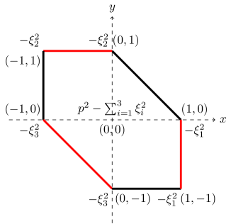
Figure 1: The Newton polyhedron associated with the sunset second Symanzik polynomial. The coordinates $(a,b)$ of the vertices we the powers of $x^{a}y^{b}$ and we give the value of the coefficient in $\phi_{\circleddash}(p^{2},\underline{\xi}^{2},x,y,1)$.

This corresponds to a maximal toric blow-up of three points in $\mathbb{P}^{2}$ leading to a del Pezzo surface of degree 6 $\mathcal{B}_{3}$. The hexagon in figure 1 resulted from the blow-up (in red on the figure) of a triangle at the points $P_{1}=[1:0:0]$, $P_{2}=[0:1:0]$ and $P_{3}=[0:0:1]$ by the mass parameters see (Bloch:2013tra, , §6) and (Bloch:2016izu, , §4). The del Pezzo 6 surfaces are rigid.

Notice that the external momentum $p^{2}$ appears only in the centre of the Newton polytope making this variable special.

One can construct a non-compact Calabi-Yau three-fold $\mathcal{M}_{\circleddash}$ defined as the anti-canonical hypersurface over the del Pezzo surface $\mathcal{B}_{3}$. This non-compact three-fold is obtained as follows (Bloch:2016izu, , §5). Consider the Laurent polynomial

$$F_{\circleddash}=a+bu^{2}v^{-1}+cu^{-1}v+u^{-1}v^{-1}\phi_{\circleddash}(p^{2},\underline{\xi}^{2},x_{1},x_{2},x_{3}),$$ (247)

with $a,b,c\in\mathbb{C}^{*}$. Its Newton polytope $\Delta$ is the convex hull of $\{(0,0,2,-1),\break(0,0,-1,1),\Delta_{\circleddash}\times(-1,-1)\}$ where $\Delta_{\circleddash}$ is the Newton polytope given by the hexagon in figure 1. The newton polytope $\Delta$ is reflexive because its polar polytope $\Delta^{\circ}:=\{y\in\mathbb{R}^{4}|\langle y,x\rangle\geq-1,\forall x\in\Delta\}=\textrm{convex\leavevmode\nobreak\ hull}\{(0,0,1,0),(0,0,0,1),6\Delta^{\circ}_{\circleddash}\times(-2,-3)\}$ is integral. Notice that for the sunset polytope is self-dual $\Delta_{\circleddash}=\Delta^{\circ}_{\circleddash}$. A triangulation of $\Delta$ gives a complete toric fan on $\Delta^{\circ}$, which then provides Fano variety $\mathbb{P}_{\Delta}$ of dimension four Coxtoric . For general $a,b,c$ and the generic physical parameters $p^{2},\xi_{1}^{2},\xi_{2}^{2},\xi_{3}^{2}$ in the sunset graph polynomial, the singular compactification $\mathcal{M}_{\circleddash}:=\overline{\{F=0\}}$ is a smooth Calabi-Yau three-fold. This non-compact Calabi-Yau three-fold can be seen as a limit of compact Calabi-Yau three-fold following the approach of CKYZ to local mirror symmetry. One can consider a semi-stably degenerating a family of elliptically-fibered Calabi-Yau three-folds $\mathcal{M}_{z}$ to a singular compactification $\mathcal{M}_{\circleddash}$ for $z=0$ and to compare the asymptotic Hodge theory of this B-model to that of the mirror (elliptically fibered) A-model Calabi-Yau $\mathcal{M}_{\circleddash}^{\circ}$. Both $\mathcal{M}_{\circleddash}$ and $\mathcal{M}_{\circleddash}^{\circ}$ are elliptically fibered over the del Pezzo of degree 6 $\mathcal{B}_{3}$. Under the mirror map we have the isomorphism of A- and B-model $\mathbb{Z}$-variation of Hodge structure Bloch:2016izu

$$H^{3}(\mathcal{M}_{z_{0}})\cong H^{even}(\mathcal{M}^{\circ}_{q_{0}})\,.$$ (248)

This situation is not unique to the two-loop sunset. The sunset graph have a reflexive polytopes containing the origin. The origin of the polytope is associated with the coefficient $p^{2}-\sum_{i=1}^{n}\xi_{i}^{2}$, and plays a very special role. The ambient space of the sunset polytope defines a Calabi-Yau hypersurfaces (the anti-canonical divisor defines a Gorenstein toric Fano variety). Therefore they are a natural home for Batyrev’s mirror symmetry techniques Batyrev94 .

Local mirror symmetry

Putting this into practise means recasting the computation in §4.2 and the mirror symmetry description in (Bloch:2016izu, , §7) in the language of Huang:2013yta , matching the computation of the Gromov-Witten prepotential in (Huang:2013yta, , §6.6).

The first step is to remark that the holomorphic $(3,0)$ period of Calabi-Yau three-fold $\mathcal{M}_{\circleddash}$ reduces to the third period $R_{0}$ once integrated on a vanishing cycle (Hosono:2006ga, , Appendix A), (Katz:1996fh, , §4) and (Bloch:2016izu, , §5.7)

$$\int_{\rm vanishing\leavevmode\nobreak\ cycle}\textrm{Res}_{F_{\circleddash}=0}\left({1\over F_{\circleddash}}{du\wedge dv\wedge\wedge dx_{1}\wedge dx_{2}\over uvx_{1}x_{2}}\right)\propto R_{0}(p^{2},\underline{\xi}^{2}),$$ (249)

where $F_{\circleddash}$ is given in (247) and $R_{0}(p^{2},\underline{\xi}^{2})$ is given in (223). This second period is related to the analytic period near $p^{2}=\infty$ by $\pi_{\circleddash}^{(2)}(p^{2},\underline{\xi}^{2})={d\over dp^{2}}R_{0}(p^{2},\underline{\xi}^{2})$.

The Gromov-Witten invariant evaluated in (229) section 4.2 are actually the BPS numbers for the del Pezzo 6 case evaluated in (Huang:2013yta, , §6.6) since

$$\sum_{\ell_{1}+\ell_{2}+\ell_{3}=\ell>0\atop(\ell_{1},\ell_{2},\ell_{3})\in{\mathbb{N}}^{3}\backslash(0,0,0)}N_{\ell_{1},\ell_{2},\ell_{3}}R_{0}^{\ell}\,\prod_{i=1}^{3}\xi_{i}^{2\ell_{i}}=\!\!\!\!\!\!\!\!\!\!\sum_{(\tilde{\ell}_{1},\tilde{\ell}_{2},\tilde{\ell}_{3})\in{\mathbb{N}}^{3}\backslash(0,0,0)}\!\!\!\!\!\!\!\!\!\!n_{\tilde{\ell}_{1},\tilde{\ell}_{2},\tilde{\ell}_{3}}\textrm{Li}_{3}(\prod_{i=1}^{3}\xi_{i}^{2\tilde{\ell}_{i}}e^{\tilde{\ell}_{i}R_{0}}),$$ (250)

where we used the covering relation (228). With the following identifications $Q_{1}=1$, $Q_{2}=\xi_{1}^{2}e^{R_{0}}$, $Q_{3}=\xi_{2}^{2}e^{R_{0}}$ and $Q_{4}=\xi_{3}^{2}e^{R_{0}}$, the expression in (250) reproduces the local genus 0 prepotential $F_{0}=F_{0}^{\textrm{c}lass}+\sum_{\boldsymbol{\beta}\in H^{2}(\mathcal{M},\mathbb{Z})}n^{\boldsymbol{\beta}}_{g}\textrm{Li}_{3}(\prod_{r=1}^{4}Q_{r}^{\beta_{r}})$ computed in (Huang:2013yta, , eq.(6.51)) with $F_{0}^{\textrm{c}lass}=\prod_{i=1}^{3}(R_{0}+\log(\xi_{i}^{2}))$ in our case.

From the complex structure of the elliptic curve we define the dual period $\pi_{1}(p^{2},\underline{\xi}^{2})=2i\pi\tau\pi_{\circleddash}^{(2)}(p^{2},\underline{\xi}^{2})$ one the other homology cycle. Which gives the dual third period $R_{1}$, such that $\pi_{1}^{(2)}(p^{2},\underline{\xi}^{2})={d\over dp^{2}}R_{1}(p^{2},\underline{\xi}^{2})$. This dual period $R_{1}$ is therefore identified with the derivative of local prepotential $F_{0}$

$$2i\pi R_{1} ={\partial\over\partial R_{0}}\,F_{0}$$ (251)

$$=\sum_{1\leq i<j\leq 3}(R_{0}+\log(\xi_{i}^{2}))(R_{0}+\log(\xi_{j}^{2}))-\!\!\!\!\!\!\!\!\sum_{\ell_{1}+\ell_{2}+\ell_{3}=\ell>0\atop(\ell_{1},\ell_{2},\ell_{3})\in\mathbb{N}^{3}\backslash\{0,0,0\}}\!\!\!\!\!\!\!\!\!\ell N_{\ell_{1},\ell_{2},\ell_{3}}\prod_{i=1}^{3}\xi_{i}^{2\ell_{i}}e^{\ell_{i}R_{0}}\,,$$

as shown in (Bloch:2016izu, , theorem 6.1) and (Bloch:2016izu, , Corollary 6.3). With these identifications it is not difficult to see that the sunset Feynman integral is actually given by the Legendre transform of $R_{1}$

$$I_{\circleddash}(p^{2},\underline{\xi}^{2})=-{2i\pi}\pi_{\circleddash}^{(2)}(p^{2},\underline{\xi}^{2})\left({\partial R_{1}\over\partial R_{0}}R_{0}-R_{1}\right)\,.$$ (252)

This shows the relation between the sunset Feynman integral computes the local Gromov-Witten prepotential. The local mirror symmetry map $Q\leftrightarrow q$ given in the relations (237) and (245) maps the B-model expression, where the sunset Feynman integral is a elliptic dilogarithm function of the complex structure $\log(q)/(2i\pi)$ of the elliptic curve and the A-model expansion in terms of the Kähler moduli $Q_{i}$.

5 Conclusion

In this text we have reviewed the toric approach to the evaluation of the maximal cut of Feynman integrals and the derivation of the minimal order differential operator acting on the Feynman integral. On the particular example of the sunset integral we have shown that the Feynman integral can take two different but equivalent forms. One form is an elliptic polylogarithm but it can as well expressed as standard trilogarithm. We have explained that mirror symmetry can be used to evaluate around the point where $p^{2}=\infty$. The expressions there makes explicit all the mass parameters. One remarkable fact is that the computation can be done using the existing technology of mirror symmetry developed in other physical Hosono:1993qy ; CKYZ ; Huang:2013yta or mathematics Doran:2011ti contexts. This analysis extends naturally to the higher loop sunset integrals DNV . The elliptic polylogarithm representation generalises to other two-loop integrals like the kite integral Adams:2016xah ; Bogner:2017vim ; Bogner:2018uus or the all equal masses three-loop sunset Bloch:2014qca . This representation leads to fast numerical evaluation Bogner:2017vim . But it has the disadvantage of hiding all the physical parameters in the geometry of the elliptic curve. The expression using the trilogarithm has the advantage of making all the mass parameters explicit and generalising to all loop orders since the expansion of the higher-loop sunset graphs around $p^{2}=\infty$ is expected to involve polylogarithms of order $l$ at $l$-loop order Doran:2011ti ; DNV .

References

• (1) J. R. Andersen et al., “Les Houches 2017: Physics at TeV Colliders Standard Model Working Group Report,” arXiv:1803.07977 [hep-ph].
• (2) D. Neill and I. Z. Rothstein, “Classical Space-Times from the S Matrix,” Nucl. Phys. B 877 (2013) 177 doi:10.1016/j.nuclphysb.2013.09.007 [arXiv:1304.7263 [hep-th]].
• (3) N. E. J. Bjerrum-Bohr, J. F. Donoghue and P. Vanhove, “On-Shell Techniques and Universal Results in Quantum Gravity,” JHEP 1402 (2014) 111 doi:10.1007/JHEP02(2014)111 [arXiv:1309.0804 [hep-th]].
• (4) F. Cachazo and A. Guevara, “Leading Singularities and Classical Gravitational Scattering,” arXiv:1705.10262 [hep-th].
• (5) A. Guevara, “Holomorphic Classical Limit for Spin Effects in Gravitational and Electromagnetic Scattering,” arXiv:1706.02314 [hep-th].
• (6) N. E. J. Bjerrum-Bohr, P. H. Damgaard, G. Festuccia, L. Planté and P. Vanhove, “General Relativity from Scattering Amplitudes,” arXiv:1806.04920 [hep-th].
• (7) O. V. Tarasov, “Hypergeometric Representation of the Two-Loop Equal Mass Sunrise Diagram,” Phys. Lett. B 638 (2006) 195 doi:10.1016/j.physletb.2006.05.033 [hep-ph/0603227].
• (8) S. Bauberger, F. A. Berends, M. Bohm and M. Buza, “Analytical and Numerical Methods for Massive Two Loop Selfenergy Diagrams,” Nucl. Phys. B 434 (1995) 383 doi:10.1016/0550-3213(94)00475-T [hep-ph/9409388].
• (9) D. H. Bailey, J. M. Borwein, D. Broadhurst and M. L. Glasser, “Elliptic Integral Evaluations of Bessel Moments,” J. Phys. A 41 (2008) 205203 doi:10.1088/1751-8113/41/20/205203 [arXiv:0801.0891 [hep-th]].
• (10) D. Broadhurst, “Elliptic Integral Evaluation of a Bessel Moment by Contour Integration of a Lattice Green Function,” arXiv:0801.4813 [hep-th].
• (11) D. Broadhurst, “Feynman Integrals, L-Series and Kloosterman Moments,” Commun. Num. Theor. Phys. 10 (2016) 527 doi:10.4310/CNTP.2016.v10.n3.a3 [arXiv:1604.03057 [physics.gen-ph]].
• (12) M. Caffo, H. Czyz and E. Remiddi, “The Pseudothreshold Expansion of the Two Loop Sunrise Selfmass Master Amplitudes,” Nucl. Phys. B 581 (2000) 274 doi:10.1016/S0550-3213(00)00274-1 [hep-ph/9912501].
• (13) S. Laporta and E. Remiddi, “Analytic Treatment of the Two Loop Equal Mass Sunrise Graph,” Nucl. Phys. B 704 (2005) 349 [hep-ph/0406160].
• (14) L. Adams, C. Bogner and S. Weinzierl, “The Two-Loop Sunrise Graph with Arbitrary Masses in Terms of Elliptic Dilogarithms,” arXiv:1405.5640 [hep-ph].
• (15) L. Adams, C. Bogner and S. Weinzierl, “The two-loop sunrise integral around four space-time dimensions and generalisations of the Clausen and Glaisher functions towards the elliptic case,” J. Math. Phys.  56 (2015) no.7, 072303 doi:10.1063/1.4926985 [arXiv:1504.03255 [hep-ph]].
• (16) L. Adams, C. Bogner and S. Weinzierl, “The iterated structure of the all-order result for the two-loop sunrise integral,” J. Math. Phys.  57 (2016) no.3, 032304 doi:10.1063/1.4944722 [arXiv:1512.05630 [hep-ph]].
• (17) L. Adams, C. Bogner and S. Weinzierl, “A walk on sunset boulevard,” PoS RADCOR 2015 (2016) 096 doi:10.22323/1.235.0096 [arXiv:1601.03646 [hep-ph]].
• (18) L. Adams and S. Weinzierl, “On a Class of Feynman Integrals Evaluating to Iterated Integrals of Modular Forms,” arXiv:1807.01007 [hep-ph].
• (19) L. Adams, E. Chaubey and S. Weinzierl, “From Elliptic Curves to Feynman Integrals,” arXiv:1807.03599 [hep-ph].
• (20) S. Bloch, M. Kerr and P. Vanhove, “Local Mirror Symmetry and the Sunset Feynman Integral,” Adv. Theor. Math. Phys. 21 (2017) 1373 doi:10.4310/ATMP.2017.v21.n6.a1 [arXiv:1601.08181 [hep-th]].
• (21) V.V. Batyrev, “Dual polyhedra and mirror symmetry for CalabiYau hypersurfaces in toric varieties,” J. Algebr. Geom. 3, 493-535 (1994)
• (22) S. Hosono, A. Klemm, S. Theisen and S. T. Yau, “Mirror Symmetry, Mirror Map and Applications to Calabi-Yau Hypersurfaces,” Commun. Math. Phys. 167 (1995) 301 doi:10.1007/BF02100589 [hep-th/9308122].
• (23) T.-M. Chiang, A. Klemm, S.-T. Yau, and E. Zaslow, “Local mirror symmetry: calculations and interpretations,” Adv. Theor. Math. Phys.  3 (1999) 495 doi:10.4310/ATMP.1999.v3.n3.a3 [hep-th/9903053].
• (24) M. X. Huang, A. Klemm and M. Poretschkin, “Refined Stable Pair Invariants for E-, M- and $[p,Q]$-Strings,” JHEP 1311 (2013) 112 doi:10.1007/JHEP11(2013)112 [arXiv:1308.0619 [hep-th]].
• (25) C.F. Doran and M. Kerr, “Algebraic K-theory of toric hypersurfaces”, Communications in Number Theory and Physics (2011) 5(2), 397–600
• (26) P. Vanhove, “The Physics and the Mixed Hodge Structure of Feynman Integrals,” Proc. Symp. Pure Math. 88 (2014) 161 doi:10.1090/pspum/088/01455 [arXiv:1401.6438 [hep-th]].
• (27) C. Bogner and S. Weinzierl, “Feynman Graph Polynomials,” Int. J. Mod. Phys. A 25 (2010) 2585 [arXiv:1002.3458 [hep-ph]].
• (28) P. Tourkine, “Tropical Amplitudes,” arXiv:1309.3551 [hep-th].
• (29) O. Amini, S. Bloch, J. I. B. Gil and J. Fresan, “Feynman Amplitudes and Limits of Heights,” Izv. Math. 80 (2016) 813 doi:10.1070/IM8492 [arXiv:1512.04862 [math.AG]].
• (30) E. R. Speer, “Generalized Feynman Amplitudes,” vol. 62 of Annals of Mathematics Studies. Princeton University Press, New Jersey, Apr., 1969.
• (31) A. Primo and L. Tancredi, “On the Maximal Cut of Feynman Integrals and the Solution of Their Differential Equations,” Nucl. Phys. B 916 (2017) 94 doi:10.1016/j.nuclphysb.2016.12.021 [arXiv:1610.08397 [hep-ph]].
• (32) A. Primo and L. Tancredi, “Maximal Cuts and Differential Equations for Feynman Integrals. an Application to the Three-Loop Massive Banana Graph,” Nucl. Phys. B 921 (2017) 316 doi:10.1016/j.nuclphysb.2017.05.018 [arXiv:1704.05465 [hep-ph]].
• (33) J. Bosma, M. Sogaard and Y. Zhang, “Maximal Cuts in Arbitrary Dimension,” JHEP 1708 (2017) 051 doi:10.1007/JHEP08(2017)051 [arXiv:1704.04255 [hep-th]].
• (34) H. Frellesvig and C. G. Papadopoulos, “Cuts of Feynman Integrals in Baikov Representation,” JHEP 1704 (2017) 083 doi:10.1007/JHEP04(2017)083 [arXiv:1701.07356 [hep-ph]].
• (35) K. G. Chetyrkin and F. V. Tkachov, “Integration by Parts: the Algorithm to Calculate Beta Functions in 4 Loops,” Nucl. Phys. B 192 (1981) 159. doi:10.1016/0550-3213(81)90199-1
• (36) O. V. Tarasov, “Generalized Recurrence Relations for Two Loop Propagator Integrals with Arbitrary Masses,” Nucl. Phys. B 502 (1997) 455 doi:10.1016/S0550-3213(97)00376-3 [hep-ph/9703319].
• (37) O. V. Tarasov, “Methods for Deriving Functional Equations for Feynman Integrals,” J. Phys. Conf. Ser. 920 (2017) no.1, 012004 doi:10.1088/1742-6596/920/1/012004 [arXiv:1709.07058 [hep-ph]].
• (38) P. Griffiths, “On the Periods of Certain Rational Integrals: I.” The Annals of Mathematics 1969, 90, 460.
• (39) D. Cox and S. Katz, “Mirror symmetry and algebraic geometry,” Mathematical Surveys and Monographs 68 (1999), American Mathematical Society, Providence, RI doi:10.1090/surv/068
• (40) T. Bitoun, C. Bogner, R. P. Klausen and E. Panzer, “Feynman Integral Relations from Parametric Annihilators,” arXiv:1712.09215 [hep-th].
• (41) Decker, W.; Greuel, G.-M.; Pfister, G.; Schönemann, H.: Singular 4-1-1 — A computer algebra system for polynomial computations. http://www.singular.uni-kl.de (2018).
• (42) I.M. Gelfand, M.M. Kapranov, A.V. Zelevinsky, “Generalized Euler Integrals and A-Hypergeometric Functions”, Advances in Math. 84 (1990), 255-271
• (43) I.M. Gelfand, M.M. Kapranov, A.V. Zelevinsky, “Discriminants, Resultants and Multidimensional Determinants”, Birkhäuser Boston, 1994
• (44) V.V. Batyrev, “Variations of the mixed hodge structure of affine hypersurfaces in algebraic tori”, Duke Mathematical Journal 69 2, 349-409, (1993)
• (45) V.V. Batyrev and D.A. Cox, “On the Hodge Structure of Projective Hypersurfaces in Toric Varieties”, Duke Mathematical Journal 75 2, 293–338, (1994)
• (46) S. Hosono, A. Klemm and S. Theisen, “Lectures on mirror symmetry,” Lect. Notes Phys.  436 (1994) 235 doi:10.1007/3-540-58453-6$\_$13 [hep-th/9403096].
• (47) C. Closset, “Toric geometry and local Calabi-Yau varieties: An Introduction to toric geometry (for physicists),” arXiv:0901.3695 [hep-th].
• (48) J. Stienstra, Jan, “GKZ hypergeometric structures”, arXiv:math/0511351
• (49) V. V. Batyrev and D. van Straten, “Generalized hypergeometric functions and rational curves on Calabi-Yau complete intersections in toric varieties,” Commun. Math. Phys.  168 (1995) 493 doi:10.1007/BF02101841 [alg-geom/9307010].
• (50) S. Hosono, “GKZ Systems, Gröbner Fans, and Moduli Spaces of Calabi-Yau Hypersurfaces,”, Birkhäuser Boston, Boston, MA, (1998)
• (51) S. Hosono, A. Klemm, S. Theisen and S. T. Yau, “Mirror Symmetry, Mirror Map and Applications to Complete Intersection Calabi-Yau Spaces,” Nucl. Phys. B 433 (1995) 501 [AMS/IP Stud. Adv. Math. 1 (1996) 545] doi:10.1016/0550-3213(94)00440-P [hep-th/9406055].
• (52) E. Cattani, “Three lectures on hypergeometric functions”, (2006)
• (53) F. Beukers, “Monodromy of A-hypergeometric functions," Journal für die Reine und Angewandte Mathematik, 718 183–206 (2016)
• (54) J. Stienstra, “Resonant Hypergeometric Systems and Mirror Symmetry,” alg-geom/9711002,
• (55) C. Doran, A.Y. Novoseltsev, and P. Vanhove, work in progress.
• (56) L. Adams, C. Bogner, and S. Weinzierl, “The Two-Loop Sunrise Graph with Arbitrary Masses,” arXiv:1302.7004 [hep-ph].
• (57) P. Candelas, X. C. de la Ossa, P. S. Green and L. Parkes, “A Pair of Calabi-Yau Manifolds as an Exactly Soluble Superconformal Theory,” Nucl. Phys. B 359 (1991) 21 [AMS/IP Stud. Adv. Math.  9 (1998) 31]. doi:10.1016/0550-3213(91)90292-6
• (58) D. R. Morrison, “Picard-Fuchs Equations and Mirror Maps for Hypersurfaces,” AMS/IP Stud. Adv. Math.  9 (1998) 185 [hep-th/9111025].
• (59) H.A. Verrill, H A, “Sums of squares of binomial coefficients, with applications to Picard-Fuchs equations,” math/0407327,
• (60) S. Bloch and P. Vanhove, “The Elliptic Dilogarithm for the Sunset Graph,” J. Number Theor. 148 (2015) 328 doi:10.1016/j.jnt.2014.09.032 [arXiv:1309.5865 [hep-th]].
• (61) S. Bloch, M. Kerr and P. Vanhove, “A Feynman Integral via Higher Normal Functions,” Compos. Math. 151 (2015) no.12, 2329 doi:10.1112/S0010437X15007472 [arXiv:1406.2664 [hep-th]].
• (62) F.C.S. Brown and A. Levin, “Multiple Elliptic Polylogarithms”, arXiv:1110.6917
• (63) J. Broedel, C. Duhr, F. Dulat and L. Tancredi, “Elliptic Polylogarithms and Iterated Integrals on Elliptic Curves. Part I: General Formalism,” JHEP 1805 (2018) 093 doi:10.1007/JHEP05(2018)093 [arXiv:1712.07089 [hep-th]].
• (64) J. Broedel, C. Duhr, F. Dulat and L. Tancredi, “Elliptic Polylogarithms and Iterated Integrals on Elliptic Curves Ii: an Application to the Sunrise Integral,” Phys. Rev. D 97 (2018) no.11, 116009 doi:10.1103/PhysRevD.97.116009 [arXiv:1712.07095 [hep-ph]].
• (65) J. Broedel, C. Duhr, F. Dulat, B. Penante and L. Tancredi, “Elliptic Symbol Calculus: from Elliptic Polylogarithms to Iterated Integrals of Eisenstein Series,” arXiv:1803.10256 [hep-th].
• (66) J. Broedel, C. Duhr, F. Dulat, B. Penante and L. Tancredi, “From Modular Forms to Differential Equations for Feynman Integrals,” arXiv:1807.00842 [hep-th].
• (67) J. Broedel, C. Duhr, F. Dulat, B. Penante and L. Tancredi, “Elliptic Polylogarithms and Two-Loop Feynman Integrals,” arXiv:1807.06238 [hep-ph].
• (68) E. Remiddi and L. Tancredi, “An Elliptic Generalization of Multiple Polylogarithms,” Nucl. Phys. B 925 (2017) 212 doi:10.1016/j.nuclphysb.2017.10.007 [arXiv:1709.03622 [hep-ph]].
• (69) W. Fulton, "Introduction to Toric Varieties, Annals of Mathematics Studies (1993), Princeton University Press
• (70) D.A. Cox, J.B. Little and H.K. Schenck,“Toric Varieties”, Graduate Studies in Mathematics (Book 124), American Mathematical Society (July 7, 2011)
• (71) S. Bloch, H. Esnault and D. Kreimer, “On Motives associated to graph polynomials,” Commun. Math. Phys.  267 (2006) 181 doi:10.1007/s00220-006-0040-2 [math/0510011 [math-ag]].
• (72) S. Hosono, “Central charges, symplectic forms, and hypergeometric series in local mirror symmetry,” Mirror Symmetry V, 405–439, ed. Yui, Noriko and Yau, Shing-Tung and Lewis, James, American Mathematical Society (2006)
• (73) S. H. Katz, A. Klemm and C. Vafa, “Geometric Engineering of Quantum Field Theories,” Nucl. Phys. B 497 (1997) 173 doi:10.1016/S0550-3213(97)00282-4 [hep-th/9609239].
• (74) J. Stienstra, “Mahler Measure Variations, Eisenstein Series and Instanton Expansions,” in Mirror symmetry V, AMS/IP Studies in Advanced Mathematics, vol. 38, eds Yui, N., Yau, S.-T. and Lewis, J. D. (International Press & American Mathematical Society, Providence, RI, 2006), 139-150. [arXiv:math/0502193]
• (75) L. Adams, C. Bogner, A. Schweitzer and S. Weinzierl, “The Kite Integral to All Orders in Terms of Elliptic Polylogarithms,” J. Math. Phys. 57 (2016) no.12, 122302 doi:10.1063/1.4969060 [arXiv:1607.01571 [hep-ph]].
• (76) C. Bogner, A. Schweitzer and S. Weinzierl, “Analytic Continuation and Numerical Evaluation of the Kite Integral and the Equal Mass Sunrise Integral,” Nucl. Phys. B 922 (2017) 528 doi:10.1016/j.nuclphysb.2017.07.008 [arXiv:1705.08952 [hep-ph]].
• (77) C. Bogner, A. Schweitzer and S. Weinzierl, “Analytic Continuation of the Kite Family,” arXiv:1807.02542 [hep-th].