Generalized Solitary Waves in the Gravity-Capillary Whitham Equation

Abstract.

We study the existence of traveling wave solutions to a unidirectional shallow water model which incorporates the full linear dispersion relation for both gravitational and capillary restoring forces. Using functional analytic techniques, we show that for small surface tension (corresponding to Bond numbers between $0$ and ${1}/{3}$) there exists small amplitude solitary waves that decay to asymptotically small periodic waves at spatial infinity. The size of the oscillations in the far field are shown to be small beyond all algebraic orders in the amplitude of the wave. We also present numerical evidence, based on the recent analytical work of Hur & Johnson, that the asymptotic end states are modulationally stable for all Bond numbers between $0$ and $1/3$.

1. Introduction

1.1. “Full dispersion” models

It is well known that the Korteweg-de Vries (KdV) equation

(1) $$u_{t}+\sqrt{gd}\left(1+\frac{1}{6}d^{2}\partial_{x}^{2}\right)u_{x}+uu_{x},$$

approximates the full water wave problem in the small amplitude, long wavelength regime [26, Section 7.4.5] [34] [35] [11]. Here, $u(x,t)$ corresponds to the fluid height at spatial position $x$ at time $t$, $d$ corresponds to the undisturbed depth of the fluid, and $g$ is the acceleration due to gravity. At least in part, the agreement in this asymptotic regime can be understood by noting that the phase speed of the water wave problem expands for $|kd|\ll 1$ as

$$c_{ww}(k):=\pm\sqrt{g\frac{\tanh(kd)}{k}}=\pm\sqrt{gd}\left(1-\frac{1}{6}k^{2}d^{2}\right)+\mathcal{O}(|kd|^{4}),$$

so that the KdV phase speed agrees to second order in $|kd|$ with that of the full water wave problem.

The KdV equation admits both solitary and periodic traveling wave solutions which are nonlinearly stable in appropriate senses [8] [31] and these results have pointed the way towards (at least some) similar results for the full water wave problem [6] [30]. Naturally, however, the KdV phase speed is a terrible approximation of $c_{ww}$ for even moderate frequencies. It should come as no surprise then that KdV fails to exhibit many high-frequency phenomena such as wave breaking – the evolutionary formation of bounded solutions with infinite gradients – and peaking – the existence of bounded, steady solutions with a singular point, such as a peak or a cusp.

The above observations led Whitham [39] to state “It is intriguing to know what kind of simpler mathematical equations (than the physical problem) could include [peaking and breaking].” In response to his own question, Whitham put forward the model

(2) $$u_{t}+\left(\mathcal{W}_{gd}u+u^{2}\right)_{x}=0,\quad u=u(x,t)\in{\mathbb{R}},\ x\in{\mathbb{R}},\ t\in{\mathbb{R}},$$

where here $\mathcal{W}$ is a Fourier multiplier operator on $L^{2}({\mathbb{R}})$ defined via

$$\mathcal{F}\left(\mathcal{W}_{gd}f\right)(k)=\sqrt{\frac{g\tanh(kd)}{k}}~{}\widehat{f}(k):$$

see [39, p. 477] By construction, the above pseudodifferential equation, modernly referred to as the “Whitham equation” or “full dispersion equation”, has a phase speed that agrees exactly with that of the full water wave problem. Since (2) balances both the full water wave dispersion with a canonical shallow water nonlinearity, Whitham conjectured that the equation (2) would be capable of predicting both breaking and peaking of waves.

And in fact it does. The Whitham equation (2) has recently been shown to exhibit wave breaking [22], as well as to admit both periodic [16] and solitary [15, 40] waves. In particular, in [12, 13], the authors conducted a detailed global bifurcation analysis of periodic traveling waves for (2) and concluded that the branch of smooth periodic waves terminates in a non-trivial cusped solution – bounded solution with unbounded derivative– that is monotone and smooth on either side of the cusp. Additionally, its well-posedness was addressed in [14], and in [23] it was shown that (2) bears out the famous Benjamin-Feir, or modulational, instability of small amplitude periodic traveling waves; see also the related numerical work [33] on the stability of large amplitude periodic waves. Taken together it is clear that, regardless of its rigorous relation to the full water wave problem, the fully dispersive model (2) admits many interesting high-frequency phenomena known to exist in the full water wave problem.

1.2. Including surface tension

It is thus natural to consider the existence and behavior of solutions when additional physical effects are included. In this paper, we incorporate surface tension and consider the following pseudodifferential equation

(3) $$u_{t}+({\mathcal{M}}_{gd\tau}u+u^{2})_{x}=0.$$

Here, $u$, $x$, and $t$ are as in (2) above, and $\mathcal{M}_{gd\tau}$ is a Fourier multiplier operator on $L^{2}({\mathbb{R}})$ with symbol

$$m_{gd\tau}(k)=\sqrt{\left(g+\tau k^{2}\right){\tanh(kd)\over k}}.$$

This symbol gives exactly the phase speed for the full gravity-capillary wave problem in the irrotational setting [25, 39]. The parameter $\tau>0$ is the coefficient of surface tension, while both $g$ and $d$ are as in (2). The properties of the symbol $m_{gd\tau}$ above depend on the non-dimensional ratio

$$\beta:=\tau/gd^{2},$$

which is referred to as the Bond number. When $\beta>1/3$, corresponding to “strong” surface tension, the phase speed $m_{gd\tau}(k)$ is monotone increasing for $k>0$ with high-frequency asymptotics $m_{gd\tau}(k)\approx|\tau k|^{1/2}$ for $|k|\gg 1$, while for “weak” surface tension, corresponding to $0<\beta<1/3$, $m_{gd\tau}(k)$ has a unique positive global minimum, after which it is monotonically increasing with the same high-frequency behavior: see Figure 1. Concerning its relation to the full water wave equations, see [9], where there the author studies the accuracy of (3) in modeling real-world experiments of waves on shallow water.

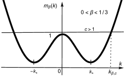
(a)    (b)  

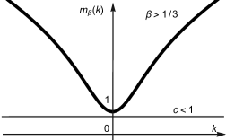
Figure 1. Schematic drawings of the linear phase speed $m_{\beta}(k)$ associated to (3) for both (a) small surface tension, corresponding to $\beta\in(0,1/3)$, and (b) large surface tension, corresponding to $\beta>1/3$.

In the full gravity-capillary wave problem with large surface tension (i.e. $\beta>1/3$) there exist subcritical solitary waves of depression (that is, they are asymptotically zero but with a unique critical point corresponding to a strictly negative absolute minimum). See, for instance, [1, 3]. When $\beta\in(0,1/3)$, however, considerably less is known about the existence of genuinely localized solitary waves. What is known is that supercritical generalized solitary waves (also called nanopterons) exist in this setting. That is, waves that are roughly the superposition of a solitary wave and a (co-propagating) periodic wave of substantially smaller amplitude, dubbed “the ripple.” See [36] [5]. In this paper, we establish analogs of these results for the gravity-capillary Whitham equation (3). We also note that the existence and stability of periodic traveling waves in (3) have recently been investigated in [24, 32]. In Section 5 below, we will apply these stability results to make observations concerning the stability of the generalized solitary waves constructed here.

1.3. Formal computations and the main results

A routine nondimensionalization of (3) converts it to

(4) $$u_{t}+\left(\mathcal{M}_{\beta}u+u^{2}\right)_{x}=0,$$

where $\mathcal{M}_{\beta}$ is the Fourier multiplier operator with symbol

(5) $$m_{\beta}(k):=\sqrt{\left(1+\beta k^{2}\right){\tanh(k)\over k}}.$$

We will henceforth be working with this version of the system. Substituting the traveling wave ansatz $u(x,t)=w(x-ct)$ into (3) yields, after one integration the nonlocal profile equation

(6) $$({\mathcal{M}}_{\beta}-c)w+w^{2}=0.$$

We are interested in long wavelength/small amplitude solutions of (6). Consequently we expect the wave speed $c$ to be close to the long wave speed $c_{lw}$, which in the nondimensionalized problem is exactly one. And so for $0<\epsilon\ll 1$, we make a “long wave/small amplitude/nearly critical” scaling of (6) by setting

(7) $$c=1+{\gamma_{\beta}}\epsilon^{2}\quad\text{and}\quad w(y)=\epsilon^{2}W(\epsilon y).$$

In the above we have made the (convenient) choice

$$\gamma_{\beta}:=-{1\over 2}m_{\beta}^{\prime\prime}(0)={1-3\beta\over 6}.$$

Consequently, if $\beta>1/3$ the solutions we are looking for are slightly subcritical, since $\gamma_{\beta}<0$. If $\beta\in(0,1/3)$ then the solutions are supercritical. After applying (7), (6) becomes

(8) $${({\mathcal{M}}^{\epsilon}_{\beta}-1-\gamma_{\beta}\epsilon^{2})}W+\epsilon^{2}W^{2}=0$$

where ${\mathcal{M}}^{\epsilon}_{\beta}$ is a Fourier multiplier with symbol $m_{\beta}(\epsilon K)$.

For $0<\epsilon\ll 1$ we have the expansion

(9) $$m_{\beta}(\epsilon K)=1-\gamma_{\beta}\epsilon^{2}K^{2}+{\mathcal{O}}(\epsilon^{4}K^{4}).$$

With the usual Fourier correspondence of $\partial_{X}$ and $iK$, the above indicates the following formal expansion:

(10) $${\mathcal{M}}_{\beta}^{\epsilon}=1+\gamma_{\beta}\epsilon^{2}\partial_{X}^{2}+{\mathcal{O}}(\epsilon^{4}\partial_{X}^{4}).$$

Therefore the (rescaled) profile equation (8) formally looks like

(11) $$\left(\gamma_{\beta}W^{\prime\prime}-\gamma_{\beta}W+{\mathcal{O}}(\epsilon^{2})\right)+\epsilon^{2}W^{2}=0.$$

Putting $\epsilon=0$, it follows that the solution satisfies the ODE

(12) $$W^{\prime\prime}-W+\gamma_{\beta}^{-1}W^{2}=0.$$

We immediately recognize (12) as the profile equation associated with solitary wave solutions of the (suitably rescaled) KdV equation (1). In particular, (12) admits a unique non-trivial even solution in $L^{2}({\mathbb{R}})$ given by

$$\sigma_{\beta}(X):={3\gamma_{\beta}\over 2}\operatorname{sech}^{2}\left({X\over 2}\right)={1-3\beta\over 4}\operatorname{sech}^{2}\left({X\over 2}\right).$$

Note that $\sigma_{\beta}(X)$ is positive when $\beta\in(0,1/3)$ and negative when $\beta>1/3$, corresponding to solitary waves of elevation and depression, respectively.

Our main goal is to analyze to how $\sigma_{\beta}$ deforms for $0<\epsilon\ll 1$. The main difficulty in the analysis is that the expansion (9) is not uniform in $K$ and, as a consequence, that the ODE (12) is necessarily singularly perturbed by the $\mathcal{O}(\epsilon^{2})$ terms in (11).

It turns out that when $\beta>1/3$ there is a straightforward way to “desingularize” the problem. The main observation is that the multiplier for the operator ${\mathcal{M}}_{\beta}-c$ is non-zero for all wave numbers when $c<1$ (i.e. is subcritical) when $\beta>1/3$. Therefore the linear part of (6) can be inverted. Doing so and then implementing the scaling (7) results in a system which is not singularly perturbed in $\epsilon$ and one can use the implicit function theorem to continue the solution $\sigma_{\beta}$ to $\epsilon>0$. In the recent paper by Stefanov & Wright [40] this strategy (which was inspired by [19, 20]) was deployed for a class of pseudodifferential equations which includes (6) when $\beta>1/3$. Their main result can be directly applied here. We explain this in greater detail in Section 3 but, for now, here is our result:

Corollary 1.

There exist subcritical solitary waves of depression for (4) when the capillary effects are strong. Specifically, for all $\beta>1/3$ and all $\epsilon$ sufficiently close to zero, there exists a small amplitude, localized, smooth, even function $R_{\epsilon}$ such that

$$w_{\epsilon}(x)=-\left({3\beta-1\over 4}\right)\epsilon^{2}\operatorname{sech}^{2}\left(\epsilon x\over 2\right)+R_{\epsilon}(\epsilon x)\quad\text{and}\quad c_{\epsilon}=1-\left({3\beta-1\over 6}\right)\epsilon^{2}$$

solve (6). For any $r\geq 0$ there exists $C_{r}>0$ such that

$$\|R^{(r)}_{\epsilon}\|_{L^{2}({\mathbb{R}})}\leq C_{r}\epsilon^{4}.$$

$R_{\epsilon}$ is the unique function with the aforementioned properties.

On the other hand, when $\beta\in(0,1/3)$ a similar desingularization will not work. In Figure 1, note that when $\beta\in(0,1/3)$ and $c>1$ (i.e. is supercritical) there is a unique $k_{\beta,c}>0$ at which

(13) $$m_{\beta}(\pm k_{\beta,c})-c=0.$$

Thus ${\mathcal{M}}_{\beta}-c$ cannot be inverted; the situation becomes more complicated. What occurs is that when $\epsilon>0$ the main pulse $\sigma_{\beta}$, through a sort of weak resonance, excites a very small amplitude periodic wave with frequency close to $k_{\beta,c}$. The end result is a generalized solitary wave as described above. See Figure 2 for a sketch of the solution. Our proof is modeled on the one devised by Beale in [5] to study traveling waves in the full gravity-capillary problem (and which has subsequently been deployed to study generalized solitary waves in other contexts in [17] [18] [21] [2]). The proof is found in Section 4. Here is our result:

Theorem 2.

There exist supercritical generalized solitary waves for (4) when the capillary effects are weak. Specifically, for all $\beta\in(0,1/3)$ and all $\epsilon$ sufficiently close to zero, there exist smooth, even functions $R_{\epsilon}$ and $P_{\epsilon}$ such that

(14) $$w_{\epsilon}(x)=\left({1-3\beta\over 4}\right)\epsilon^{2}\operatorname{sech}^{2}\left(\epsilon x\over 2\right)+R_{\epsilon}(\epsilon x)+P_{\epsilon}(x)\quad\text{and}\quad c_{\epsilon}=1+\left({1-3\beta\over 6}\right)\epsilon^{2}$$

solve (6). The functions $R_{\epsilon}$ and $P_{\epsilon}$ have the following properties.

1. $R_{\epsilon}(X)$ is an exponentially localized function of small amplitude. In particular, there is a constant $q_{*}>0$ such that for all $r\geq 0$ there exists $C_{r}>0$ for which

   $$\|\cosh^{q_{*}}(\cdot)R^{(r)}_{\epsilon}(\cdot)\|_{L^{\infty}({\mathbb{R}})}\leq C_{r}\epsilon^{4}.$$

2. $P_{\epsilon}(x)$ is a periodic solution of (6) whose frequency is approximately $k_{\beta,c_{\epsilon}}$ and whose amplitude is small beyond all algebraic orders. Specifically, there is a constant $\delta>0$ such that the frequency of $P_{\epsilon}$ lies in the interval $[k_{\beta,c_{\epsilon}}-\delta\epsilon,k_{\beta,c_{\epsilon}}+\delta\epsilon]$ and for all $r\geq 0$ there is a constant $C_{r}>0$ for which

   $$\|P_{\epsilon}\|_{L^{\infty}({\mathbb{R}})}\leq C_{r}\epsilon^{r}.$$

Moreover, this solution is unique in the sense that no other pair $(R_{\epsilon},P_{\epsilon})$ leads to a solution of (6) of the form (14) which meets all the criteria stated in (i) and (ii).

Figure 2. This is a cartoon illustrating our main result Theorem 2.

The waves $w_{\epsilon}$ constructed in Theorem 2 consist of a localized cure connecting two asymptotically small oscillatory end states. In addition to the existence result presented above, we also discuss how this rough “decomposition” can be combined with recent work [24] to provide insight into the possible stability of these waves. While we do not arrive at any definitive stability results here, we hope our study spurs additional work.

Remark 1.

We also point out the work [4], where the author uses direct variational arguments to prove the existence of localized solutions to a large class of pseudo-partial differential equations that contains (4) for all values of $\beta>0$. In the case of small surface tension, however, the fact that his waves have phase speeds slightly less than the global minimia of the phase speed $m$ (hence, are necessiarly subcritical with respect to the long-wave phase speed $m_{\beta}(0)$). Labeling $k^{*}$ the (strictly positive) frequency where the global minima of $m$ is achieved, it follows that the localized waves constructed in [4] are in fact modulated solitary waves, taking approximately the form $\phi(x)\cos(k^{*}x)$ for some localized function $\phi\in L^{2}({\mathbb{R}})$.

Acknowledgments

The authors would like to thank Mats Ehrnström, Mark Groves, Miles Wheeler, Atanas Stefanov and Mathias Arnesen for useful conversations about this work. The work of M.A.J. was partially supported by the NSF under grant DMS-1614785. The work of J.D.W. was partially supported by the NSF under grant DMS-1511488.

2. Conventions

Here we specify the notation for the function spaces we will be using along with some other conventions.

2.1. Periodic functions

We let $W^{r,p}_{\text{per}}:=W^{r,p}{(\mathbb{T}})$ be the usual “$r,p$” Sobolev space of $2\pi$-periodic functions. We denote $L^{p}_{\text{per}}:=W^{0,p}_{\text{per}}$ and $H^{r}_{\text{per}}:=W^{r,2}_{\text{per}}$. Put

(15) $$E^{r}_{\text{per}}:=H^{r}_{{\text{per}}}\cap\left\{\text{even functions}\right\}.$$

By $C^{r}_{\text{per}}$ we mean the space of $r-$times differentiable $2\pi$-periodic functions and $C^{\infty}_{\text{per}}$ is the space of smooth $2\pi$-periodic functions.

2.2. Functions on ${\mathbb{R}}$:

We let $W^{r,p}:=W^{r,p}({\mathbb{R}})$ be the usual “$r,p$” Sobolev space of functions defined on ${\mathbb{R}}$. For $q\in{\mathbb{R}}$ put

(16) $$W^{r,p}_{q}:=\left\{u\in L^{2}({\mathbb{R}}):\cosh^{q}(x)u(x)\in W^{r,p}({\mathbb{R}})\right\}.$$

These are Banach spaces with the naturally defined norm. If we say a function is “exponentially localized” we mean that it is in one of these spaces with $q>0$.

Put $L^{p}_{q}:=W^{0,p}_{q}$, $H^{r}:=W^{r,2}$ and $H^{r}_{q}:=W^{r,2}_{q}$ and denote

$$\|f\|_{r,q}:=\|f\|_{H^{r}_{q}}:=\|\cosh(\cdot)^{q}f(\cdot)\|_{H^{r}({\mathbb{R}})}.$$

We let

(17) $$E^{r}_{q}:=H^{r}_{q}\cap\left\{\text{even functions}\right\}.$$

2.3. Spaces of operators

For Banach spaces $X$ and $Y$ we let $B(X,Y)$ be the space of bounded linear operators from $X$ to $Y$ equipped with the usual induced topology.

2.4. Big $C$ notation:

Suppose that $Q_{1}$ and $Q_{2}$ are positive quantities (like norms) which depend upon the smallness parameter $\epsilon$, the regularity index $r$, the decay rate $q$ and some collection of elements $\eta$ which live in a Banach space $X$.

When we write “$Q_{1}\leq CQ_{2}$” we mean “there exists $C>0$, $\epsilon_{0}>0$, $q_{0}>0$, $\delta>0$ such that $Q_{1}\leq CQ_{2}$ for all $r\geq 0$, $q\in[0,q_{0}]$, $\epsilon\in(0,\epsilon_{0}]$ and $\|\eta\|_{X}\leq\delta_{0}$.” In particular, the constant does not depend on anything.

When we write “$Q\leq C_{r}f(\epsilon)$” we mean “there exists $\epsilon_{0}>0$, $q_{0}>0$, $\delta_{0}>0$ such that for any $r\geq 0$ there exist $C_{r}>0$ such that $Q_{1}\leq C_{r}Q_{2}$ when $q\in[0,q_{0}]$, $\epsilon\in(0,\epsilon_{0}]$ and $\|\eta\|_{X}\leq\delta_{0}$.” In this case, the constant depends on $r$ but nothing else.

When we write “$Q\leq C_{q}f(\epsilon)$” we mean “there exists $\epsilon_{0}>0$, $q_{0}>0$, $\delta_{0}>0$ such that for any $q\in(0,q_{0}]$ there exists $C_{q}>0$ such that $Q_{1}\leq C_{q}Q_{2}$ when $r\geq 0$, $\epsilon\in(0,\epsilon_{0}]$ and $\|\eta\|_{X}\leq\delta_{0}$.” The constant depends on $q$ but nothing else.

Lastly, when we write “$Q_{1}\leq C_{r,q}Q_{2}$” we mean “there exists $\epsilon_{0}>0$, $q_{0}>0$, $\delta_{0}>0$ such that for any $r\geq 0$ and $q\in(0,q_{0}]$ there exist $C_{r,q}>0$ such that $Q_{1}\leq C_{r,q}Q_{2}$ when $\epsilon\in(0,\epsilon_{0}]$ and $\|\eta\|_{X}\leq\delta_{0}$.” That is, the constant depends on $r$ and $q$.

2.5. Fourier analysis:

We use following normalizations and notations for the Fourier transform and its inverse:

$$\widehat{f}(k):={\mathcal{F}}[f](k):={1\over 2\pi}\int_{\mathbb{R}}f(x)e^{-ikx}dx\quad\text{and}\quad{\mathchoice{{\ooalign{\hbox{\raise 6.25pt\hbox{\scalebox{1.0}[-1.0]{\lower 6.25pt\hbox{$\displaystyle\widehat{\vrule width=0.0pt,height=4.30554pt\vrule height=0.0pt,width=5.12846pt}$}}}}\cr\hbox{$\displaystyle g$}}}}{{\ooalign{\hbox{\raise 6.25pt\hbox{\scalebox{1.0}[-1.0]{\lower 6.25pt\hbox{$\textstyle\widehat{\vrule width=0.0pt,height=4.30554pt\vrule height=0.0pt,width=5.12846pt}$}}}}\cr\hbox{$\textstyle g$}}}}{{\ooalign{\hbox{\raise 5.81944pt\hbox{\scalebox{1.0}[-1.0]{\lower 5.81944pt\hbox{$\scriptstyle\widehat{\vrule width=0.0pt,height=3.01389pt\vrule height=0.0pt,width=3.58992pt}$}}}}\cr\hbox{$\scriptstyle g$}}}}{{\ooalign{\hbox{\raise 5.53241pt\hbox{\scalebox{1.0}[-1.0]{\lower 5.53241pt\hbox{$\scriptscriptstyle\widehat{\vrule width=0.0pt,height=2.15277pt\vrule height=0.0pt,width=2.56422pt}$}}}}\cr\hbox{$\scriptscriptstyle g$}}}}}(x):={\mathcal{F}}^{-1}[g](x):=\int_{\mathbb{R}}g(k)e^{ikx}dk.$$

3. Solitary waves of depression when $\beta>1/3$.

The following theorem on the existence of solitary waves in a certain class of pseudodifferential equations was proved in [40]:

Theorem 3.

Suppose that there exists $\delta_{*}>0$ such that $n:(-\delta_{*},\delta_{*})\to{\mathbb{R}}$ is $C^{2,1}$ (that is, its second derivative exists and is uniformly Lipschitz continuous) and satisfies

$$n(0)=n^{\prime}(0)=0\quad\text{and}\quad n^{\prime\prime}(0)>0.$$

Moreover suppose that $l:{\mathbb{R}}\to{\mathbb{R}}$ is even and there exists $\bar{k}>0$ which has the following properties:

1. $l(k)$ is $C^{3,1}$ (that is, its third derivative exists and is uniformly Lipschitz continuous) for $k\in[-\bar{k},\bar{k}]$.

2. $l_{2}:=\max_{|k|\leq\bar{k}}l^{\prime\prime}(k)<0.$

3. $l_{1}:=\sup_{k\geq\bar{k}}l(k)<l(0).$

Let $\mathcal{L}$ be the Fourier multiplier operator with symbol $l(k)$. Then there exists $\epsilon_{0}>0$, so that for every $\epsilon\in(0,\epsilon_{0})$, there is a solution $(\phi,v)\in E^{1}_{0}\times{\mathbb{R}}$ of

(18) $$\left(\mathcal{L}-v\right)\phi+n(\phi)=0$$

of the form

$$\phi(y)=\epsilon^{2}\Phi_{\epsilon}(\epsilon y)\quad\text{and}\quad v=l(0)-{1\over 2}l^{\prime\prime}(0)\epsilon^{2}$$

where

$$\Phi_{\epsilon}(X)=-\frac{3l^{\prime\prime}(0)}{2n^{\prime\prime}(0)}\operatorname{sech}^{2}\left(\frac{X}{2}\right)+\rho_{\epsilon}(X).$$

The function $\rho_{\epsilon}(X)\in E^{1}_{0}$ satisfies the estimate $\left\|\rho_{\epsilon}\right\|_{1,0}\leq C\epsilon^{2}.$

This theorem can be applied directly to (6) when $\beta>1/3$. Specifically, let $v=-c$, $l=-m$, $\mathcal{L}=-{\mathcal{M}}$, $\phi=-u$ and $n(\phi)=\phi^{2}$. Then (6) is transformed into (18). Clearly $n(\phi)=\phi^{2}$ meets the required hypotheses in Theorem 3. Given the graph of $m_{\beta}(k)$ in Figure 1, it is easily believed—and even true—that $l(k)=-m_{\beta}(k)$ meets all conditions (a)-(c) when $\beta>1/3$. Thus we get the conclusions of the theorem. Unwinding the very simple rescalings gives us most of Corollary 1. Note that Theorem 3 only tells us that the solutions are in $E^{1}_{0}$ whereas Corollary 1 tells us they are smooth. In this problem, however, we have the additional information that $m_{\beta}(k)$ grows like $|k|^{1/2}$ for large $|k|$ and hence ${\mathcal{M}}_{\beta}$ is “like” $\partial_{x}^{1/2}$. With this, a straightforward bootstrapping argument demonstrates that the solutions are smooth. We omit these details.

4. Generalized solitary waves when $\beta\in(0,1/3)$.

In this section we prove Theorem 2. Throughout we fix $\beta\in(0,1/3)$ and we will, for the most part, not track how quantities depend on this quantity.

4.1. A necessary solvability condition

We begin our proof of Theorem 2 by doing something that is doomed to fail. Nevertheless, we believe that understanding the mechanism behind this failure is an important step in the journey to the proof of Theorem 2. Throughout, $r\geq 1$ (a regularity index) is fixed but arbitrary and $q>0$ (a decay rate) is taken to be sufficiently small.

To this end, we first attempt to construct solutions of the nonlocal profile equation (8) for $0<\epsilon\ll 1$ of the form

(19) $$W_{\epsilon}(X)=\sigma_{\beta}(X)+R(X),$$

where $R=R(\cdot;\epsilon)$ is to be some small, smooth, even function in $E^{r}_{q}$. Inserting this ansatz into (8) leads to the following equation for $R$:

(20) $${{\mathcal{L}}_{\epsilon}}R+2\sigma_{\beta}R={\mathbf{J}}_{0}+{\mathbf{J}}_{1}$$

Here

$${\mathcal{L}}_{\epsilon}:=\epsilon^{-2}({\mathcal{M}}_{\beta}^{\epsilon}-1-\gamma_{\beta}\epsilon^{2}),\quad{\mathbf{J}}_{0}=-\sigma_{\beta}^{2}-\epsilon^{-2}({\mathcal{M}}_{\beta}^{\epsilon}-1-\gamma_{\beta}\epsilon^{2})\sigma_{\beta}\quad\text{and}\quad{\mathbf{J}}_{1}:=-R^{2}.$$

Note that $\epsilon^{2}\mathcal{L}_{\epsilon}$ is simply the linearization of (8) about the trivial solution $u=0$. ${\mathbf{J}}_{1}$ is obviously quadratic in the unknown $R$, thus we obtain the following estimates via Sobolev embedding when $r\geq 1$:

(21) $$\|{\mathbf{J}}_{1}\|_{r,q}\leq C_{r}\|R\|_{r,q}^{2}\quad\text{and}\quad\|{\mathbf{J}}_{1}-\widetilde{{\mathbf{J}}}_{1}\|_{r,q}\leq C_{r}\left(\|R\|_{r,q}+\|\widetilde{R}\|_{r,q}\right)\|R-\widetilde{R}\|_{r,q}.$$

Above, by $\widetilde{{\mathbf{J}}}_{1}$ we simply mean the quantity ${\mathbf{J}}_{1}$ evaluated at a function $\widetilde{R}$ instead of at $R$.

As for ${\mathbf{J}}_{0}$, it is a small forcing term. From its definition and that fact that $\sigma_{\beta}(X)$ solves (12) we see that

(22) $$\begin{split}{\mathbf{J}}_{0}=&\gamma_{\beta}(\sigma_{\beta}^{\prime\prime}-\sigma_{\beta})-\epsilon^{-2}\left({\mathcal{M}}_{\beta}^{\epsilon}-1-\gamma_{\beta}\epsilon^{2}\right)\sigma_{\beta}\\ =&-\epsilon^{-2}({\mathcal{M}}_{\beta}^{\epsilon}-1-\gamma_{\beta}\epsilon^{2}\partial_{X}^{2})\sigma_{\beta}.\end{split}$$

Then the formal expansion of ${\mathcal{M}}_{\beta}^{\epsilon}$ in (10) indicates that ${\mathbf{J}}_{0}\sim\epsilon^{2}\partial_{X}^{4}\sigma_{\beta}$. This argument can be made rigorous by way of Fourier analysis:

Lemma 4.

There exists $q_{0}>0$ so that for any $q\in[0,q_{0}]$ and $r\geq 0$ we have

(23) $$\|{\mathbf{J}}_{0}\|_{r,q}\leq C_{r}\epsilon^{2}.$$

The proof is in the Appendix.

To attempt to solve the nonlinear problem (20), we first consider the solvability of the nonhomogeneous linear equation

(24) $$\mathcal{L}_{\epsilon}R+2\sigma_{\beta}R=F$$

for $F\in E^{r}_{q}$. Assuming the continuous solvability of (24) on $E^{r}_{q}$, we could then attempt to solve the nonlinear equation (20) through iteration.

Recall from (13) that for $\beta\in(0,1/3)$ and $c>1$ there exists unique $k_{\beta,c}>0$ such that $m_{\beta}(\pm k_{\beta,c})=c$. This implies that the symbol

(25) $$l_{\epsilon}(K):=\epsilon^{-2}\left(m_{\beta}(\epsilon K)-1-\gamma_{\beta}\epsilon^{2}\right)$$

associated to the linear operator $\mathcal{L}_{\epsilon}$ satisfies

(26) $$l_{\epsilon}(\pm K_{\epsilon})=0$$

where

(27) $$K_{\epsilon}:={k_{\beta,1+\gamma_{\beta}\epsilon^{2}}\over\epsilon}.$$

From the above considerations it is easy to conclude that $K_{\epsilon}=\mathcal{O}(1/\epsilon)$ and is the unique frequency for which (26) occurs.

Taking the Fourier transform of (24) and evaluating at $K_{\epsilon}$ implies that (24) is only solvable provided that $R$ and the forcing $F$ satisfy $2\widehat{\sigma_{\beta}R}(K_{\epsilon})=\widehat{F}(K_{\epsilon})$. For a generic $F\in E^{r}_{q}$, it follows that the single unknown $R$ is required to solve two equations, hence the linear problem (24) is overdetermined. Consequently, the above method of constructing a localized solution of (8) of the form (19) fails.

4.2. Beale’s method

Beale encountered nearly the same obstacle encountered in Section 4.1 in his work on the full gravity-capillary water wave problem [5]. In his investigation, he made the remarkable observation that just as the special frequency $K_{\epsilon}$ causes difficulties at the linear level, it also points to a way out. Indeed, observe that the lack of solvability of the linear forced equation (24) stems from (26) which, when written on the spatial side, simply states that the linear problem ${\mathcal{L}}_{\epsilon}P=0$ has a solution of the form $P=\cos(K_{\epsilon}X).$ Beale used this observation to motivate a refinement of the ansatz (19) that incorporates a family of small amplitude, nonlinear periodic traveling waves associated to the governing profile equation which are roughly given by $a\cos(K_{\epsilon}X)$ where $|a|\ll 1$. By using the amplitude of this oscillation as an additional free variable, he was able to overcome the above difficulties.

In order to adapt Beale’s method to the present case, we begin by recalling that, for each fixed $0<\epsilon\ll 1$, the nonlinear profile equation (8) admits a family of small amplitude, spatially periodic solutions with frequencies close to $K_{\epsilon}$. Indeed, the following result follows from the analysis of [24]:

Theorem 5.

Fix $\beta\in(0,1/3)$. There exists $\epsilon_{0}>0$, $\alpha_{0}>0$ and a mapping

(28) $$\begin{split}[-\alpha_{0},\alpha_{0}]\times(0,\epsilon_{0}]&\longrightarrow{\mathbb{R}}\times C_{\text{per}}^{\infty}\\ (a,\epsilon)&\longmapsto(K_{\epsilon}^{a},\phi_{\epsilon}^{a})\\ \end{split}$$

with the following properties:

• For each $\epsilon\in(0,\epsilon_{0}]$, the function $W(X)=a\phi_{\epsilon}^{a}(K_{\epsilon}^{a}X)$ solves (8) for all $|a|\leq\alpha_{0}$.

• $\phi_{\epsilon}^{0}(X)=\cos(X)$ and $K_{\epsilon}^{0}=K_{\epsilon}$.

• There exists $C>0$ such that $0<\epsilon\leq\epsilon_{0}$ and $|a|,|{\widetilde{a}}|\leq\alpha_{0}$ imply

  (29) $$|K_{\epsilon}^{a}-K_{\epsilon}^{{\widetilde{a}}}|\leq C|a-{\widetilde{a}}|.$$

• For all $r\geq 0$ there exists $C_{r}>0$ such that $0<\epsilon\leq\epsilon_{0}$ and $|a|,|{\widetilde{a}}|\leq\alpha_{0}$ imply

  (30) $$\|\phi^{a}_{\epsilon}-\phi^{{\widetilde{a}}}_{\epsilon}\|_{H^{r}_{\text{per}}}\leq C_{r}|a-{\widetilde{a}}|.$$

Following Beale, we refine the ansatz (19) by including one of the above small amplitude waves. Specifically, introducing the notation

(31) $${\Phi_{\epsilon}^{a}(X)}:=\phi_{\epsilon}^{a}(K_{\epsilon}^{a}X)$$

we attempt to construct solutions of the profile equation (8) for $0<\epsilon\ll 1$ of the form

(32) $$W_{\epsilon}(X)=\sigma_{\beta}(X)+a{\Phi_{\epsilon}^{a}(X)}+R(X)$$

where now both $R\in E^{r}_{q}$ and $a\in{\mathbb{R}}$ are unknowns. Inserting the refined ansatz (32) into (8) gives the equation

$${\mathcal{L}}_{\epsilon}R+2\sigma_{\beta}R+2a\sigma_{\beta}\Phi_{\epsilon}^{a}+2a\Phi^{a}_{\epsilon}R={\mathbf{J}}_{0}+{\mathbf{J}}_{1}$$

where here $\mathcal{L}_{\epsilon}$, ${\mathbf{J}}_{0}$ and ${\mathbf{J}}_{1}$ are as before. Note that the term $a\Phi^{a}_{\epsilon}R$ is clearly nonlinear in the unknowns $a$ and $R$. The term $a\sigma_{\beta}\Phi^{a}_{\epsilon}$ however has an $\mathcal{O}(a)$ term coming from the fact that $\Phi^{0}_{\epsilon}(X)=\cos(K_{\epsilon}X)$. Incorporating this additional linear term on the left hand side of leads to the nonlinear equation

(33) $${\mathcal{L}}_{\epsilon}R+2\sigma_{\beta}R+2a\sigma_{\beta}\Phi_{\epsilon}^{0}={\mathbf{J}}_{0}+{\mathbf{J}}_{1}+{\mathbf{J}}_{2}+{\mathbf{J}}_{3}$$

where here we have

$${\mathbf{J}}_{2}:=-2a\sigma_{\beta}\left(\Phi_{\epsilon}^{a}-\Phi_{\epsilon}^{0}\right)\quad\text{and}\quad{\mathbf{J}}_{3}=-2a\Phi^{a}_{\epsilon}R.$$

Given (29) and (30) we see that ${\mathbf{J}}_{2}$ is nonlinear in the sense that it is morally ${\mathcal{O}}(a^{2})$. This leads to:

Lemma 6.

There exists $\epsilon_{0}>0$ and $q_{0}>0$ such that, for all $r\geq 0$, $q\in[0,q_{0}]$ and $\epsilon\in(0,\epsilon_{0}]$ we have

(34) $$\|{\mathbf{J}}_{2}\|_{r,q}\leq C_{r}\epsilon^{-r}a^{2}\quad\text{and}\quad\|{\mathbf{J}}_{2}-\widetilde{{\mathbf{J}}}_{2}\|_{r,q}\leq C_{r}\epsilon^{-r}(|a|+|\widetilde{a}|)|a-\widetilde{a}|.$$

As for ${\mathbf{J}}_{3}$, it is roughly ${\mathcal{O}}(aR)$. Specifically:

Lemma 7.

There exists $\epsilon_{0}>0$ and $q_{0}>0$ such that, for all $r\geq 0$, $q\in[0,q_{0}]$ and $\epsilon\in(0,\epsilon_{0}]$ we have

(35) $$\left\{\begin{aligned} \|{\mathbf{J}}_{3}\|_{r,q}&\leq C_{r}\epsilon^{-r}|a|\|R\|_{r,q}\\ &\quad\text{and}\quad\|{\mathbf{J}}_{3}-\widetilde{{\mathbf{J}}}_{3}\|_{r,0}\leq C_{r,q}\epsilon^{-r}\left((\|R\|_{r,q}+\|\widetilde{R}\|_{r,q})|a-\widetilde{a}|+(|a|+|\widetilde{a}|)\|R-\widetilde{R}\|_{r,0}\right).\end{aligned}\right.$$

In both (34) and (35) above, $\widetilde{{\mathbf{J}}}_{l}$ simply represents the quantity ${\mathbf{J}}_{l}$ evaluated at $\widetilde{R}$ and $\widetilde{a}$. An important feature of these estimates is that there is a mismatch in the decay rates of the pieces in the estimate in (35)(ii): specifically, on the left we measure in $H^{r}_{0}$ but the right requires $R$ and $\widetilde{R}$ to be in $H^{r}_{q}$ with $q>0$. In particular, the constant $C_{r,q}$ diverges as $q\to 0^{+}$. We provide the justification for Lemmas 6 and 7 in the Appendix.

Our goal is now to resolve the nonlinear equations (33) for $R$ and $a$. As in Section 4.1, we will proceed by first considering the solvability of the associated nonhomogeneous linear equation. After we have shown that this can be continuously solved, we solve the full nonlinear equation (33) through iteration.

4.3. The linear problem

The left hand side of (33) is linear in $R$ and $a$. We claim it is a bijection in an appropriate sense. Specifically we have the following linear solvability result.

Proposition 8.

There exists $\epsilon_{0}>0$ and $q_{0}>0$ for which the following hold when $\epsilon\in(0,\epsilon_{0}]$, $q\in(0,q_{0}]$ and $r\geq 0$. There are linear maps

$${\mathcal{R}}_{\epsilon}:E^{r}_{q}\longrightarrow E^{r+1/2}_{q}\quad\text{and}\quad{\mathcal{A}}_{\epsilon}:E^{r}_{q}\longrightarrow{\mathbb{R}}$$

such that

(36) $${\mathcal{L}}_{\epsilon}R+2\sigma_{\beta}R+2a\sigma_{\beta}\Phi_{\epsilon}^{0}=G\in E^{r}_{q}$$

if and only if

$$R={\mathcal{R}}_{\epsilon}G\quad\text{and}\quad a={\mathcal{A}}_{\epsilon}G.$$

Moreover these maps are continuous and satisfy the estimates

$$\|{\mathcal{R}}_{\epsilon}\|_{B(E^{r}_{q},E^{r+1/2}_{q})}\leq C_{r,q}\quad\text{and}\quad\|{\mathcal{A}}_{\epsilon}\|_{B(E^{r}_{q},{\mathbb{R}})}\leq C_{r,q}\epsilon^{r}.$$

Remark 2.

It is important to note that the size of $\mathcal{A}_{\epsilon}$ is directly related to the (Sobolev) smoothness of the forcing function $G$. This observation will be important in our coming work.

Proof.

Recalling (26), we first see that to solve (36) requires the linear solvability condition

(37) $$2\widehat{\sigma_{\beta}R}(K_{\epsilon})+2a\widehat{\sigma_{\beta}\Phi_{\epsilon}^{0}}(K_{\epsilon})=\widehat{G}(K_{\epsilon})$$

to hold. Since $\Phi_{\epsilon}^{0}(X)=\cos(K_{\epsilon}X)$ by Theorem 5, we can calculate

(38) $$\begin{split}2\widehat{\sigma_{\beta}\Phi_{\epsilon}^{0}}(K_{\epsilon})&={1\over\pi}\int_{\mathbb{R}}\sigma_{\beta}(X)\cos(K_{\epsilon}X)e^{-iK_{\epsilon}X}dX\\ &={1\over\pi}\int_{\mathbb{R}}\left({1\over 2}\sigma_{\beta}(X)+{1\over 2}\sigma_{\beta}(X)e^{-2iK_{\epsilon}X}\right)dX\\ &=\widehat{\sigma_{\beta}}(0)+\widehat{\sigma_{\beta}}(2K_{\epsilon})\\ &=:\chi_{\epsilon}\end{split}$$

Note that since $\sigma_{\beta}\in L^{1}({\mathbb{R}})$ is positive, we know $\widehat{\sigma}_{\beta}(0)>0$. Moreover, the analyticity of $\sigma_{\beta}$ and the fact that $K_{\epsilon}={\mathcal{O}}(1/\epsilon)$ implies $|\widehat{\sigma_{\beta}}(2K_{\epsilon})|$ is exponentially small in $\epsilon$. Consequently $\chi_{\epsilon}$ and $\chi_{\epsilon}^{-1}$ are bounded uniformly in $\epsilon$ for $0<\epsilon\ll 1$. It follows that we can solve (37) for $a$ explicitly in terms of $G$ and $R$ as

(39) $$a=\chi_{\epsilon}^{-1}\left(\widehat{G}(K_{\epsilon})-2\widehat{\sigma_{\beta}R}(K_{\epsilon})\right),$$

thus guaranteeing that this choice of $a$ ensures the linear solvability (37) holds for a given $G\in E^{r}_{q}$, provided that we can now resolve (36) for $R$.

Before substituting (39) into (36), define the operator ${\mathcal{P}}_{\epsilon}:E^{r}_{q}\to E^{r}_{q}$ by

$${\mathcal{P}}_{\epsilon}F=F-2\widehat{F}(K_{\epsilon})\chi_{\epsilon}^{-1}\sigma_{\beta}\Phi_{\epsilon}^{0}.$$

By construction, for all $F\in E^{r}_{q}$

(40) $$\widehat{{\mathcal{P}}_{\epsilon}F}(K_{\epsilon})=0.$$

Furthermore

(41) $$\|{\mathcal{P}}_{\epsilon}\|_{B(E^{r}_{q})}\leq C_{r,q}.$$

To prove this, one needs the Riemann-Lebesgue estimate

(42) $$\left|\widehat{F}(K)\right|\leq CK^{-r}q^{-1/2}\|F\|_{r,q}$$

which holds for any $\pm K>1$ and $q>0$. See Lemma A.5 in [18] for a proof. With this, (41) follows quickly from the fact that $\Phi_{\epsilon}^{0}(X)=\cos(K_{\epsilon}X)$ and that $\chi_{\epsilon}^{-1}$ is bounded above. Specifically

$$\begin{split}\|{\mathcal{P}}_{\epsilon}F\|_{r,q}&\leq\|F\|_{r,q}+2\chi_{\epsilon}^{-1}\left|\widehat{F}(K_{\epsilon})\right|\|\sigma_{\beta}\Phi_{\epsilon}^{0}\|_{r,q}\\ &\leq\left(1+C_{q}K_{\epsilon}^{-r}\|\sigma_{\beta}\|_{r,q}\|\Phi_{\epsilon}^{0}\|_{W^{r,\infty}({\mathbb{R}})}\right)\|F\|_{r,q}\\ &\leq\left(1+C_{q}K_{\epsilon}^{-r}\|\sigma_{\beta}\|_{r,q}K_{\epsilon}^{r}\right)\|F\|_{r,q}\\ &\leq C_{r,q}\|F\|_{r,q}\end{split}$$

Substituting (39) into (36) gives the equation

(43) $${\mathcal{L}}_{\epsilon}R+{\mathcal{P}}_{\epsilon}(2\sigma_{\beta}R)={\mathcal{P}}_{\epsilon}G.$$

Given (40), the linear solvability condition coming from (26) is satisfied in (43). The next result shows that this the operator $\mathcal{L}_{\epsilon}$ is indeed continuously invertible on the range of ${\mathcal{P}}_{\epsilon}$.

Lemma 9.

There exists $q_{0}>0$ and $\epsilon_{0}>0$ such the following holds for all $q\in(0,q_{0}]$, $\epsilon\in(0,\epsilon_{0}]$ and $r\geq 0$. Suppose that $F\in E^{r}_{q}$ and $\widehat{F}(K_{\epsilon})=0$. Then there exists a unique $R\in E^{r+1/2}_{q}$, which we denote by ${\mathcal{L}}_{\epsilon}^{-1}F$, such that ${\mathcal{L}}_{\epsilon}R=F$. Finally, we have

$$\|R\|_{r+1/2,q}=\|{\mathcal{L}}_{\epsilon}^{-1}F\|_{r+1/2,q}\leq C_{r,q}\|F\|_{r,q}.$$

We provide the proof in the Appendix. Together with (40), Lemma 9 allows us to rewrite (43) as

(44) $$R+{\mathcal{L}}_{\epsilon}^{-1}{\mathcal{P}}_{\epsilon}(2\sigma_{\beta}R)={\mathcal{L}}_{\epsilon}^{-1}{\mathcal{P}}_{\epsilon}G.$$

At first glance, it is not entirely clear that we have made progress towards our goal of solving for $R$, as we have to figure out how to invert the operator $1+{\mathcal{L}}_{\epsilon}^{-1}{\mathcal{P}}_{\epsilon}(2\sigma_{\beta}\cdot)$. To make this step requires a critical feature of ${\mathcal{L}}_{\epsilon}^{-1}{\mathcal{P}}_{\epsilon}$: it is small perturbation of $-\gamma_{\beta}^{-1}(1-\partial_{X}^{2})^{-1}$. Specifically, if we put

$${\mathcal{G}}_{\epsilon}:=\epsilon^{-1}\left({\mathcal{L}}_{\epsilon}^{-1}{\mathcal{P}}_{\epsilon}+\gamma_{\beta}^{-1}(1-\partial_{X}^{2})^{-1}\right)$$

then we can establish the following result.

Lemma 10.

There exists $q_{0}>0$ and $\epsilon_{0}>0$ such that for all $q\in(0,q_{0}]$, $\epsilon\in(0,\epsilon_{0}]$ and $r\geq 0$ we have

$$\|{\mathcal{G}}_{\epsilon}\|_{B(E^{r}_{q},E^{r}_{q})}\leq C_{r,q}.$$

Again, we provide the proof of Lemma 10 in the Appendix. Notice, however that this result is not unexpected since the formal expansion (10) indicates

(45) $${\mathcal{L}}_{\epsilon}=-\gamma_{\beta}(1-\partial_{X}^{2})+{\mathcal{O}}(\epsilon^{2}).$$

Lemma 10 provides a meaningful and rigorous version of (45) and as such represents one of the keys of our analysis. Indeed, as in our discussion directly above the statement of Theorem 2, the $\mathcal{L}_{\epsilon}$ is a singular perturbation of the operator $-\gamma_{\beta}(1+\partial_{X}^{2})$, and resolving this singular limit is one of the main technical difficulties faced in the present study.

We can rewrite (46) as

(46) $$\begin{array}[t]{@{}c@{}}\underbrace{R-\gamma_{\beta}^{-1}(1-\partial_{X}^{2})^{-1}(2\sigma_{\beta}R)+2\epsilon{\mathcal{G}}_{\epsilon}(\sigma_{\beta}R)}\\ {\mathcal{S}}_{\epsilon}R\end{array}={\mathcal{L}}_{\epsilon}^{-1}{\mathcal{P}}_{\epsilon}G.$$

Using (10), we see that ${\mathcal{S}}_{0}=1-\gamma_{\beta}^{-1}(1-\partial_{X}^{2})^{-1}(2\sigma_{\beta}\cdot)$, which is recognized as as $-(1-\partial_{X}^{2})^{-1}$ applied to the linearization of the KdV profile equation (12) about the KdV solitary wave $\sigma_{\beta}$. This latter operator has been very well studied in the literature, and in particular it follows from standard Sturm-Liouville theory on $L^{2}({\mathbb{R}})$ that ${\rm ker}(S_{0})={\rm span}\{\sigma_{\beta}^{\prime}\}$. Since $\sigma_{\beta}^{\prime}$ is odd by construction, it follows that ${\mathcal{S}}_{0}$ is invertible on the class of even functions in $E^{r}_{0}({\mathbb{R}})$ for any $r>0$. Following (for instance) Appendix D.10 of [17], this observation can be extended to the weighted space $E^{r}_{q}$ via operator conjugation. Specifically:

Lemma 11.

There exists $q_{0}>0$ such that for all $r\geq 0$ and $q\in[0,q_{0}]$ the operator ${\mathcal{S}}_{0}$ is a bounded and invertible map from $E^{r}_{q}\to E^{r}_{q}$. In particular

$$\|{\mathcal{S}}_{0}\|_{B(E^{r}_{q})}+\|{\mathcal{S}}_{0}^{-1}\|_{B(E^{r}_{q})}\leq C_{r}.$$

Notice that Lemma 10 implies that ${\mathcal{S}}_{\epsilon}$ is a small regular perturbation of ${\mathcal{S}}_{0}$ and thus, for $\epsilon$ sufficiently small the operator ${\mathcal{S}}_{\epsilon}$ is invertible on $E^{r}_{q}$ as well and satisfies the estimate

$$\|{\mathcal{S}}_{\epsilon}\|_{B(E^{r}_{q})}+\|{\mathcal{S}}_{\epsilon}^{-1}\|_{B(E^{r}_{q})}\leq C_{r}.$$

Consequently, we can invert ${\mathcal{S}}_{\epsilon}$ in (46) and solve for $R$ completely in terms of $G\in E^{r}_{q}$ as

(47) $$R={\mathcal{R}}_{\epsilon}G:={\mathcal{S}}_{\epsilon}^{-1}{\mathcal{L}}_{\epsilon}^{-1}{\mathcal{P}}_{\epsilon}G.$$

Following through the above estimates we have we find that

$$\|{\mathcal{R}}_{\epsilon}\|_{B(E^{r}_{q},E^{r+1/2}_{q})}\leq C_{r,q}.$$

Furthermore, returning to (39) we find that $a$ is given in terms of $G$ as

$$a={\mathcal{A}}_{\epsilon}G:=\chi_{\epsilon}^{-1}\left(\widehat{G}(K_{\epsilon})-2\widehat{\sigma_{\beta}{\mathcal{R}}_{\epsilon}G}(K_{\epsilon})\right).$$

To estimate the size of $a$ in terms of $\epsilon$, we use (42) and the fact that $K_{\epsilon}={\mathcal{O}}(1/\epsilon)$ to get:

$$\|{\mathcal{A}}_{\epsilon}\|_{B(E^{r}_{q},{\mathbb{R}})}\leq C_{r,q}\epsilon^{r}.$$

This completes the proof of Proposition 8. ∎

4.4. Nonlinear solvability

We now return to constructing a solution of the form (32) to the nonlinear equation (33). Thanks to Proposition 8 we see that solving (33) is equivalent to solving the fixed point problem

(48) $$\begin{split}R={\mathcal{R}}_{\epsilon}\left({\mathbf{J}}_{0}+{\mathbf{J}}_{1}+{\mathbf{J}}_{2}+{\mathbf{J}}_{3}\right)=:{\bf{N}}^{1}_{\epsilon}(R,a)\\ a={\mathcal{A}}_{\epsilon}\left({\mathbf{J}}_{0}+{\mathbf{J}}_{1}+{\mathbf{J}}_{2}+{\mathbf{J}}_{3}\right)=:{\bf{N}}^{2}_{\epsilon}(R,a).\end{split}$$

on the space $E^{r}_{q}\times{\mathbb{R}}$, where here the ${\mathbf{J}}_{i}$ are defined as in Section 4.2 above. The goal is to show that in a sufficiently small neighborhood of $E^{r}_{q}\times{\mathbb{R}}$, the nonlinear system (48) has a unique solution. To this end, we begin by collecting necessary estimates on the nonlinear terms, all of which follow in a direct way by Proposition 8 and (21), (23), (34), and (35).

Proposition 12.

There exist $q_{*}>0$ and $\epsilon_{0}>0$ with the following properties. For all $r\geq 1$ there exist $\kappa_{r}>0$ such that $\epsilon\in(0,\epsilon_{0}]$ implies

(49) $$\|{\bf{N}}_{\epsilon}^{1}(R,a)\|_{r,q_{*}}\leq\kappa_{r}\left(\epsilon^{2}+\epsilon^{-r+1/2}a^{2}+\epsilon^{-r+1/2}|a|\|R\|_{r-1/2,q_{*}}+\|R\|^{2}_{r-1/2,q_{*}}\right),$$

(50) $$|{\bf{N}}_{\epsilon}^{2}(R,a)|\leq\kappa_{r}\left(\epsilon^{r+2}+a^{2}+|a|\|R\|_{r,q_{*}}+\epsilon^{r}\|R\|^{2}_{r,q_{*}}\right),$$

(51) $$\|{\bf{N}}_{\epsilon}^{1}(R,a)-{\bf{N}}_{\epsilon}^{1}(\widetilde{R},{\widetilde{a}})\|_{r,0}\leq\kappa_{r}\epsilon^{-r}(\|R\|_{r,q_{*}}+\|\widetilde{R}\|_{r,q_{*}}+|a|+|{\widetilde{a}}|)|a-{\widetilde{a}}|\\ +\kappa_{r}\left(\|R\|_{r,0}+\|\widetilde{R}\|_{r,0}+\epsilon^{-r}\left(|a|+|{\widetilde{a}}|\right)\right)\|R-\widetilde{R}\|_{r,0}$$

and

(52) $$|{\bf{N}}_{\epsilon}^{2}(R,a)-{\bf{N}}_{\epsilon}^{2}(\widetilde{R},{\widetilde{a}})|\leq\kappa_{r}(\|R\|_{r,q_{*}}+\|\widetilde{R}\|_{r,q_{*}}+|a|+|{\widetilde{a}}|)|a-{\widetilde{a}}|\\ +\kappa_{r}\epsilon^{r}\left(\|R\|_{r,q_{*}}+\|\widetilde{R}\|_{r,q_{*}}+\epsilon^{-r}\left(|a|+|{\widetilde{a}}|\right)\right)\|R-\widetilde{R}\|_{r,0}.$$

Equipped with the above estimates, we construct our small solution to (48) by a classical iterative argument. To begin, let $R_{0}:=0$, $a_{0}:=0$ and for $n\geq 0$ define

(53) $$R_{n+1}:={\bf{N}}_{\epsilon}^{1}(R_{n},a_{n})\quad\text{and}\quad a_{n+1}:={\bf{N}}_{\epsilon}^{2}(R_{n},a_{n}).$$

We first claim that for each fixed $r\geq 1$ there exists $\epsilon_{r}>0$ such that

(54) $$\|R_{n}\|_{r,q_{*}}\leq 2\kappa_{r}\epsilon^{2}\quad\text{and}\quad|a_{n}|\leq 2\kappa_{r}\epsilon^{r+2}.$$

for all $\epsilon\in(0,\epsilon_{r}]$. Here $\kappa_{r}>0$ is as in Proposition 12. The proof is by induction and the base case is obvious. For the inductive step, if we assume (54) then (53) implies by way of the estimates (49) and (50) that

$$\|R_{n+1}\|_{r,q_{*}}\leq\kappa_{r,q_{*}}\left(\epsilon^{2}+\epsilon^{-r+1/2}(2\kappa_{r,q_{*}}\epsilon^{r+2})^{2}+\epsilon^{-r+1/2}|2\kappa_{r,q_{*}}\epsilon^{r+2}|2\kappa_{r,q_{*}}\epsilon^{2}+(2\kappa_{r,q_{*}}\epsilon^{2})^{2}\right)$$

and

$$|a_{n+1}|\leq\kappa_{r,q_{*}}\left(\epsilon^{r+2}+(2\kappa_{r,q_{*}}\epsilon^{r+2})^{2}+|2\kappa_{r,q_{*}}\epsilon^{r+2}|2\kappa_{r,q_{*}}\epsilon^{2}+\epsilon^{r}(2\kappa_{r,q_{*}}\epsilon^{2})^{2}\right).$$

which, after tidying up and requiring $0<\epsilon<1$, gives the estimates

$$\|R_{n+1}\|_{r,q_{*}}\leq\kappa_{r}\epsilon^{2}\left(1+12\kappa^{2}_{r}\epsilon^{2}\right)\quad\text{and}\quad|a_{n+1}|\leq\kappa_{r}\epsilon^{r+2}\left(1+12\kappa_{r}^{2}\epsilon^{2}\right).$$

By setting

(55) $$\epsilon_{r}:={1\over\sqrt{12}\kappa_{r}},$$

then we have attained our goal of showing (54) for all $n$ when $\epsilon\in(0,\epsilon_{r}]$, with $\epsilon_{r}$ defined as in (55).

Thus, for $\epsilon$ small enough we have that $\left\{(R_{n},a_{n})\right\}_{n\geq 0}$ a bounded sequence in $E^{r}_{q_{*}}\times{\mathbb{R}}$. We now demonstrate that this sequence converges strongly in the space $E^{r}_{0}\times{\mathbb{R}}$. Using (53) together with the estimates (51) and (52) we find directly that

$$\begin{split}\|R_{n+1}-R_{n}\|_{r,0}=&\|{\bf{N}}_{\epsilon}^{1}(R_{n},a_{n})-{\bf{N}}_{\epsilon}^{1}(R_{n-1},a_{n-1})\|_{r,0}\\ \leq&\kappa_{r}\epsilon^{-r}(\|R_{n}\|_{r,q_{*}}+\|R_{n-1}\|_{r,q_{*}}+|a_{n}|+|a_{n-1}|)|a_{n}-a_{n-1}|\\ &+\kappa_{r}\left(\|R_{n}\|_{r,0}+\|R_{n-1}\|_{r,0}+\epsilon^{-r}\left(|a_{n}|+|a_{n-1}|\right)\right)\|R_{n}-R_{n-1}\|_{r,0}\\ \end{split}$$

and

$$\begin{split}|a_{n+1}-a_{n}|=&|{\bf{N}}_{\epsilon}^{2}(R_{n},a_{n})-{\bf{N}}_{\epsilon}^{2}(R_{n-1},a_{n-1})|\\ \leq&\kappa_{r}(\|R_{n}\|_{r,q_{*}}+\|R_{n-1}\|_{r,q_{*}}+|a_{n}|+|a_{n-1}|)|a_{n}-a_{n-1}|\\ &+\kappa_{r}\epsilon^{r}\left(\|R_{n}\|_{r,q_{*}}+\|R_{n-1}\|_{r,q_{*}}+\epsilon^{-r}\left(|a_{n}|+|a_{n-1}|\right)\right)\|R_{n}-R_{n-1}\|_{r,0}.\end{split}$$

Using (54) it follows from the above estimates that

$$\begin{split}\|R_{n+1}-R_{n}\|_{r,0}\leq&8\kappa^{2}_{r}\epsilon^{2}\left(\epsilon^{-r}|a_{n}-a_{n-1}|+\|R_{n}-R_{n-1}\|_{r,0}\right)\\ \end{split}$$

and

$$\begin{split}|a_{n+1}-a_{n}|\leq&8\kappa^{2}_{r}\epsilon^{2}\left(|a_{n}-a_{n-1}|+\epsilon^{r}\|R_{n}-R_{n-1}\|_{r,0}\right),\end{split}$$

valid for all $n\geq 1$ and $\epsilon\in(0,\epsilon_{r}]$. Taken together, it follows that

(56) $$\|R_{n+1}-R_{n}\|_{r,0}+\epsilon^{-r}|{a}_{n+1}-a_{n}|\leq 8\kappa^{2}_{r}\epsilon^{2}\left(\|R_{n}-R_{n-1}\|_{r,0}+\epsilon^{-r}|{a}_{n}-{a}_{n-1}|\right),$$

which, in turn, gives

$$\|R_{n+1}-R_{n}\|_{r,0}+\epsilon^{-r}|{a}_{n+1}-a_{n}|\leq\left(8\kappa^{2}_{r}\epsilon^{2}\right)^{n}\left(\|R_{1}-R_{0}\|_{r,0}+\epsilon^{-r}|{a}_{1}-{a}_{0}|\right).$$

Using the initial conditions $R_{0}=0$, $a_{0}=0$ along with (54) converts this to

$$\|R_{n+1}-R_{n}\|_{r,0}+\epsilon^{-r}|{a}_{n+1}-a_{n}|\leq 4\kappa_{r}\epsilon^{2}\left(8\kappa^{2}_{r}\epsilon^{2}\right)^{n}.$$

By the triangle inequality, it now follows that for $m,n\geq 1$ and $m>n$ we have

$$\|R_{m}-R_{n}\|_{r,0}+\epsilon^{-r}|{a}_{m}-a_{n}|\leq\sum_{k=n}^{m-1}4\kappa_{r}\epsilon^{2}\left(8\kappa^{2}_{r}\epsilon^{2}\right)^{k}.$$

Note that since since $\epsilon\in(0,\epsilon_{r}]$, with $\epsilon_{r}$ as in (55), we have that $8\kappa^{2}_{r}\epsilon^{2}<1$ and hence, using a geometric series, we find

$$\|R_{m}-R_{n}\|_{r,0}+\epsilon^{-r}|{a}_{m}-a_{n}|\leq{4\kappa_{r}\epsilon^{2}\left(8\kappa^{2}_{r}\epsilon^{2}\right)^{n}\over 1-8\kappa^{2}_{r}\epsilon^{2}}.$$

Since the right hand side converges to zero as $n\to\infty$, it follows that $\left\{(R_{n},a_{n})\right\}_{n\geq 0}$ is a Cauchy sequence in $E^{r}_{0}\times{\mathbb{R}}$. As $E^{r}_{0}\times{\mathbb{R}}$ is clearly a Hilbert space, it follows that exists $(R_{\epsilon},a_{\epsilon})\in E^{r}_{0}\times{\mathbb{R}}$ such that

(57) $$(R_{n},a_{n})\underset{E^{r}_{0}\times{\mathbb{R}}}{\longrightarrow}(R_{\epsilon},a_{\epsilon})\quad\text{as $n\to\infty$}.$$

Our next goal is to show that, in fact, the function $R_{\epsilon}$ is exponentially localized. To this end, let $q_{*}>0$ be fixed as in Proposition 12 and note that (54) implies that $\{R_{n}\}_{n\geq 0}$ is a bounded in $E^{r}_{q_{*}}$. Since $E^{r}_{q_{*}}$ is a Hilbert space it follows that we can extract a weakly convergent subsequence in $E^{r}_{q_{*}}$. Denote this weak limit as $\widetilde{R}_{\epsilon}\in E^{r}_{q_{*}}$ and note that since $E^{r}_{q_{*}}\subset E^{r}_{0}$, the same subsequence also converges weakly to $\widetilde{R}_{\epsilon}$ in the unweighted space $E^{r}_{0}$. However, since we have already shown that $R_{n}\to R_{\epsilon}$ strongly in $E^{r}_{0}$ we must have $R_{\epsilon}=\widetilde{R}_{\epsilon}$ by the uniqueness of weak limits which, in turn, immediately implies that $R_{\epsilon}\in E^{r}_{q_{*}}$, as claimed. Furthermore, since norms on Hilbert spaces are lower semi-continuous with respect to weak limits, we know from (54) that

(58) $$\|R_{\epsilon}\|_{r,q_{*}}\leq 2\kappa_{r}\epsilon^{2}\quad\text{and}\quad|a_{\epsilon}|\leq 2\kappa_{r}\epsilon^{r+2}.$$

The next step is to show that the pair $(R_{\epsilon},a_{\epsilon})\in E^{r}_{q}\times{\mathbb{R}}$ is indeed a solution of the nonlinear system (48), i.e. that

(59) $$R_{\epsilon}={\bf{N}}_{\epsilon}^{1}(R_{\epsilon},a_{\epsilon})\quad\text{and}\quad a_{\epsilon}={\bf{N}}_{\epsilon}^{2}(R_{\epsilon},a_{\epsilon}).$$

Since we know each term in the sequence $\{R_{n}\}_{n\geq 0}$ meets the bound in (54), and since we know $R_{\epsilon}$ satisfies the similar estimate (58), we can conclude from (51), (52) and (57) that

$$({\bf{N}}_{\epsilon}^{1}(R_{n},a_{n}),{\bf{N}}_{\epsilon}^{2}(R_{n},a_{n}))\underset{E^{r}_{0}\times{\mathbb{R}}}{\longrightarrow}({\bf{N}}_{\epsilon}^{1}(R_{\epsilon},a_{\epsilon}),{\bf{N}}_{\epsilon}^{2}(R_{\epsilon},a_{\epsilon}))\quad\text{as $n\to\infty$}.$$

Consequently, we can pass to the limit in the iterative scheme (53) to conclude (59). This establishes the existence component of Theorem 2.

It is also the case that $(R_{\epsilon},a_{\epsilon})$ is the unique solution of (48) which meets the estimates in (58). Indeed, if there were another pair $(\widetilde{R}_{\epsilon},{\widetilde{a}}_{\epsilon})\in E^{r}_{q}\times{\mathbb{R}}$ that satisfies both (48) and (58), then it is apparent that

$$\|R_{\epsilon}-\widetilde{R}_{\epsilon}\|_{r,0}+\epsilon^{-r}|{a}_{\epsilon}-{\widetilde{a}}_{\epsilon}|=\|{\bf{N}}_{\epsilon}^{1}(R_{\epsilon},a_{\epsilon})-{\bf{N}}_{\epsilon}^{1}(\widetilde{R}_{\epsilon},{\widetilde{a}}_{\epsilon})\|_{r,0}+\epsilon^{-r}|{\bf{N}}_{\epsilon}^{2}(R_{\epsilon},a_{\epsilon})-{\bf{N}}_{\epsilon}^{2}(\widetilde{R}_{\epsilon},{\widetilde{a}}_{\epsilon})|.$$

Using the same argument that led from (51) and (52) to (56), we find that

$$\|R_{\epsilon}-\widetilde{R}_{\epsilon}\|_{r,0}+\epsilon^{-r}|{a}_{\epsilon}-{\widetilde{a}}_{\epsilon}|\leq 8\kappa^{2}_{r}\epsilon^{2}\left(\|R_{\epsilon}-\widetilde{R}_{\epsilon}\|_{r,0}+\epsilon^{-r}|{a}_{\epsilon}-{{\widetilde{a}}}_{\epsilon}|\right).$$

which, since $8\kappa^{2}_{r}\epsilon^{2}<1$, implies $(\widetilde{R}_{\epsilon},{\widetilde{a}}_{\epsilon})=(R_{\epsilon},a_{\epsilon})$, as claimed.

It remains to discuss the smoothness of the solutions $R_{\epsilon}$ constructed above. The smoothing property imputed in (49) implies, since our solutions are fixed points, that our functions $R_{\epsilon}$ are $C^{\infty}$ by a routine bootstrap argument. But there is more to the story. Note that we left the precise value of the regularity index $r$ unspecified above; there was no restriction on its size. The uniqueness property together with the containment $E^{r+1}_{q_{*}}\subset E^{r}_{q_{*}}$ implies that the solution we construct at order $r$ coincides with the ones we construct at higher regularity, at least for $\epsilon$ small enough. This is another avenue for establishing the smoothness of the solutions, but also more than that. Note that the larger the regularity index $r$, the tighter the bound on $a_{\epsilon}$ is in (58). Thus we can conclude that $|a_{\epsilon}|\leq C_{r}\epsilon^{r}$ for all $r\geq 1$, i.e. that it is small beyond all algebraic orders of $\epsilon$. By putting $P_{\epsilon}(x)=a_{\epsilon}\Phi_{\epsilon}^{a_{\epsilon}}(x/\epsilon)$ we have proven Theorem 2.

5. Discussion on Stability

In this final section, we briefly consider the spectral stability of the generalized solitary waves constructed in Theorem 2. Specifically, we are interested in the ability of these generalized solitary waves to persist when subject to small perturbations. As we will see, a necessary condition for our small generalized solitary waves to be stable is that their oscillatory endstates be stable. This is made rigorous below by the Weyl essential spectrum theorem. The stability of the small, oscillatory endstates has recently been investigated in [24], allowing us to make observations about the stability of the patterns constructed in Theorem 2.

To begin, fix $\epsilon$ sufficiently small and note that $w_{\epsilon}$ is an equilibrium solution of the evolution equation

$$u_{t}+\partial_{x}\left(\mathcal{M}_{\beta}u-c_{\epsilon}u+u^{2}\right)=0.$$

Linearizing about the equilibrium solution $w_{\epsilon}$ leads to the following linear evolution equation:

(60) $$v_{t}+\partial_{x}\left(\mathcal{M}_{\beta}v-c_{\epsilon}v+2w_{\epsilon}v\right)=0.$$

Here we require $v(\cdot,t)\in L^{2}({\mathbb{R}})$ for all $t\geq 0$. The solution $w_{\epsilon}$ is said to be linearly stable provided solutions of (60) that begin small remain small for all time.

A first step in the study of linear stability is often to study the spectrum of the associated linear operator. Here, this corresponds to studying the spectrum of

$$L_{\epsilon}:=\partial_{x}\left(\mathcal{M}_{\beta}-c_{\epsilon}+2w_{\epsilon}\right),$$

considered as a closed, densely defined linear operator on $L^{2}({\mathbb{R}})$ with domain $H^{3/2}({\mathbb{R}})$. The wave $w_{\epsilon}$ is said to be spectrally stable provided the spectrum $\sigma(L_{\epsilon})$ does not intersect the open right half plane, i.e. provided

$$\sigma(L_{\epsilon})\cap\left\{z\in\mathbb{C}:\Re(z)>0\right\}=\emptyset.$$

Note that since the coefficients of $L_{\epsilon}$ are real-valued, the set $\sigma(L_{\epsilon})$ is symmetric about the real axis. Furthermore, since $L_{\epsilon}$ is the composition of a skew-adjoint and a self-adjoint operator, the spectrum of $L_{\epsilon}$ is invariant with respect to reflection through the origin. Together, this implies the following:

$$\lambda\in\sigma(L_{\epsilon})\quad\Rightarrow\quad\pm\lambda,~{}\pm\bar{\lambda}\in\sigma(L_{\epsilon}).$$

It follows that the pattern $w_{\epsilon}$ is spectrally stable if and only if $\sigma(L_{\epsilon})\subset{\mathbb{R}}i$.

To study the spectrum of $L$, note that from Theorem 2 the wave $w_{\epsilon}$ can be decomposed into an exponentially localized “core” $\Psi_{\epsilon}$ and the oscillatory “ripple” $P_{\epsilon}$:

$$w_{\epsilon}(x)=\Psi_{\epsilon}(x)+P_{\epsilon}(x).$$

This decomposition motivates our main observation regarding the spectral analysis of $L_{\epsilon}$, which is the content of the following:

Lemma 13.

When considered as operators on $L^{2}({\mathbb{R}})$ with domains $H^{3/2}({\mathbb{R}})$, the operator $L_{\epsilon}$ is a relatively compact perturbation of the asymptotic operator

$$\widetilde{L}_{\epsilon}:=\partial_{x}\left(\mathcal{M}_{\beta}-c+2P_{\epsilon}\right).$$

Proof.

Observe that the difference

$$\mathcal{D}_{\epsilon}:=L_{\epsilon}-\widetilde{L}_{\epsilon}=2\partial_{x}\left(\Psi_{\epsilon}~{}\cdot\right)$$

defines a closed operator on $L^{2}({\mathbb{R}})$ with domain $H^{1}({\mathbb{R}})$. Using that $\Psi_{\epsilon}$ and its derivatives decay exponentially fast at spatial infinity, the continuity of $\mathcal{D}_{\epsilon}$ as a map from $H^{3/2}({\mathbb{R}})$ to $H^{1/2}({\mathbb{R}})$, and the compactness of the embedding $H^{1/2}(I)$ into $L^{2}(I)$ for any compact interval $I\subset{\mathbb{R}}$ one can show that if $\{f_{n}\}_{n=1}^{\infty}$ is a bounded sequence in $H^{3/2}({\mathbb{R}})$, then the sequence $\{\mathcal{D}_{\epsilon}(f_{n})\}_{n=1}^{\infty}\subset L^{2}({\mathbb{R}})$ has a convergent subsequence. The claim now follows. ∎

Since the essential spectrum is stable with respect to relatively compact perturbations, it follows that the essential spectrum of $L_{\epsilon}$ acting on $L^{2}({\mathbb{R}})$ agrees with the essential spectrum of the periodic-coefficient linear operator $\widetilde{L}_{\epsilon}$ acting on $L^{2}({\mathbb{R}})$. Consequently, we can conclude the generalized solitary wave $w_{\epsilon}$ is spectrally unstable if its small amplitude, periodic oscillations are spectrally unstable. We now study the spectral stability of these oscillations.

As the operator $\widetilde{L}_{\epsilon}$ has periodic coefficients its spectrum can be studied via Floquet-Bloch theory, from which it can be easily shown that non-trivial solutions of $\widetilde{L}_{\epsilon}v=\lambda v$ can not be integrable over ${\mathbb{R}}$: at best, they can be bounded over ${\mathbb{R}}$, and hence the spectrum of $\widetilde{L}_{\epsilon}$ over $L^{2}({\mathbb{R}})$ is purely essential. In particular, it can be shown that $\sigma(\widetilde{L}_{\epsilon})$ consists of a countable number of continuous curves in $\mathbb{C}$: see [38] for details. Using Floquet-Bloch theory, it can be shown that in a sufficiently small neighborhood of the origin $\lambda=0$, the set $\sigma(\widetilde{L}_{\epsilon})$ consists of three curves, all of which pass through the origin: see [24]. If all three of these curves are confined to the imaginary axis, we say that the background periodic wave $P_{\epsilon}$ is modulationally stable, while it is modulationally unstable otherwise.

The modulational stability of the small amplitude periodic traveling wave solutions $P_{\epsilon}$ was recently studied in [24]. There, the authors use rigorous spectral perturbation theory to establish the following result.

Theorem 14 (Modulational Stability Index).

Fix $\beta\in(0,1/3)$ and $\epsilon>0$ sufficiently small. Then the $2\pi/{k_{\epsilon}^{*}}$- periodic traveling wave $P_{\epsilon}$ is modulationally unstable if $\Delta_{\rm MI}(k_{\epsilon}^{*})<0$, where

$$\Delta_{\rm MI}(z):=\frac{(zm_{\beta}(z))^{\prime\prime}\left((zm_{\beta}(z))^{\prime}-m_{\beta}(0)\right)}{m_{\beta}(z)-m_{\beta}(2z)}~{}~{}\Delta_{\rm BF}(z),$$

and $\Delta_{\rm BF}(z):=2(m_{\beta}(z)-m_{\beta}(2z))+((zm_{\beta}(z))^{\prime}-m(0))$. Furthermore, $P_{\epsilon}$ is modulationally stable if $\Delta_{MI}(k_{\epsilon}^{*})>0$.

It follows from Theorem 14 that there are four mechanisms which can cause a change in the sign of the modulational instability index $\Delta_{\rm MI}$, hence signaling a change in the modulational stability of the wave $P_{\epsilon}$:

• the group velocity $c_{g}(k):=(km_{\beta}(k))^{\prime}$ attains an extremum at some wave number $k$, i.e. $c_{g}^{\prime}(k)=0$;

• the group velocity coincides with the phase velocity $c_{p}(k):=m_{\beta}(k)$ of the limiting long wave at $k=0$, resulting in a resonance between long and short waves, i.e. $(km_{\beta}(k))^{\prime}=m(0)$;

• the phase velocities of the fundamental mode and the second harmonic coincide, i.e. $m(k)=m(2k)$;

• $\Delta_{BF}(k)=0$.

It is interesting to note that possibilities (1)-(3) are purely linear, not depending on any nonlinear effects. Note since the waves $P_{\epsilon}$ are necessarily supercritical, the third possibility above can never occur. Furthermore, the formula for $\Delta_{\rm MI}$ is completely explicit in terms of the phase speed $m_{\beta}$, and hence can be analyzed numerically.

Figure 3. The modulational stability diagram, written in coordinates $k$ versus $k\sqrt{\beta}$-plane, for the small amplitude, periodic traveling waves of (3). To interpret, for fixed $\beta>0$ one must envision a line through the origin with slope $\sqrt{\beta}$. Here, “$S$” and “$U$” denote regions of modulational stability and instability, respectively. The dark blue curve represents the function $\beta\to k_{\beta,c_{0}}$, corresponding to the frequencies of the oscillatory (linear) wave $P_{0}$.

According to Theorem 2, the frequency of the oscillatory wave $P_{\epsilon}$ is given by $k_{\epsilon}^{*}\approx k_{\beta,c_{\epsilon}}+\mathcal{O}(\epsilon)$. Consequently, at first pass we can gain insight into the modulational stability of $P_{\epsilon}$ by calculating $\Delta_{\rm MI}(k_{\beta,c_{0}})$. Performing such a numerical calculation indicates that $\beta\mapsto\Delta_{\rm MI}(k_{\beta,c_{0}})>0$ for all $\tau\in(0,1/3)$: see Figure 3.

From the above numerical observations, it seems likely that the oscillatory, asymptotic end states $P_{\epsilon}$ of the generalized solitary waves $w_{\epsilon}$ are modulationally stable for all $\tau\in(0,1/3)$ and $\epsilon>0$ sufficiently small. We note that this serves as evidence that the waves $w_{\epsilon}$ could be spectrally stable to localized perturbations in $L^{2}({\mathbb{R}})$. Of course, one must additionally study the spectral stability of the oscillatory tail $P_{\epsilon}$ away from the origin in order to have a complete picture of the essential spectrum of $w_{\epsilon}$. Provided that this analysis indicates stability, it then remains to understand the effect of the localized core $\Psi_{\epsilon}$ on the spectral properties of the linearized operator. We consider these as very interesting questions that will hopefully be studied elsewhere.

Appendix A Proofs of Technical Estimates

In this Appendix, we prove a number of technical lemmas used throughout the paper. To prove Lemma 4, we need the following general result:

Lemma 15.

Suppose that $h(Z)$ is a complex valued function with the following properties:

1. $h(Z)$ is analytic on the closed strip $\overline{\Sigma}_{q}=\left\{|\Im Z|\leq q\right\}\subset{\mathbb{C}}$ where $q>0$;

2. there exists $0\leq n\in\mathbb{Z}$ and $c_{*}>0$ such that $Z\in\overline{\Sigma}_{q}$ imply that $|h(Z)|\leq c_{*}|z|^{n}$.

Then the Fourier multiplier operator ${\mathcal{H}}$ with symbol $h$ is a bounded map from $H^{r+n}_{q}$ into $H^{r}_{q}$ and we have

(61) $$\|{\mathcal{H}}f\|_{r,q}\leq Cc_{*}\|f^{(n)}\|_{r,q}.$$

The constant $C>0$ does not depend on $h$, $r$, $q$, $n$, or $f$.

Proof.

One can show that

$$|f|_{r,q}:=\sqrt{\int_{\mathbb{R}}(1+|K|^{2})^{r}\left(|\widehat{f}(K+iq)|^{2}+|\widehat{f}(K-iq)|^{2}\right)dK}$$

is equivalent to $\|f\|_{r,q}$ by means of the Paley-Wiener theorem (see, for instance, [7]). The constants in the equivalence can be taken independent of both $r$ and $q$. Then we have, using the equivalence and the estimate in part (ii):

$$\begin{split}\|{\mathcal{H}}f\|_{r,q}\leq&C|{\mathcal{H}}f|_{r,q}\\ =&C\sqrt{\int_{\mathbb{R}}(1+|K|^{2})^{r}\left(|h(K+iq)\widehat{f}(K+iq)|^{2}+|h(K+iq)\widehat{f}(K-iq)|^{2}\right)dK}\\ \leq&Cc_{*}\sqrt{\int_{\mathbb{R}}(1+|K|^{2})^{r}|K|^{2n}\left(|\widehat{f}(K+iq)|^{2}+|\widehat{f}(K-iq)|^{2}\right)dK}\\ \leq&Cc_{*}|f^{(n)}|_{r,q}\\ \leq&Cc_{*}\|f^{(n)}\|_{r,q}.\end{split}$$

∎

Now we can prove Lemma 4:

Proof.

(Lemma 4) A straightforward Taylor’s theorem argument shows that there exist $Q>0$ and $c_{*}>0$ such that

$$|\Im_{\beta}(z)|\leq Q\implies\left|m_{\beta}(z)-1+\gamma_{\beta}z^{2}\right|\leq c_{*}|z|^{4}.$$

This implies that

$$|\Im_{\beta}(Z)|\leq Q/\epsilon\implies\epsilon^{-2}\left|m_{\beta}(\epsilon Z)-1+\gamma_{\beta}\epsilon^{2}Z^{2}\right|\leq c_{*}\epsilon^{2}|Z|^{4}.$$

Note that $\epsilon^{-2}({\mathcal{M}}_{\beta}^{\epsilon}-1-\gamma_{\beta}\epsilon^{2}\partial_{X}^{2})$ is a Fourier multiplier with symbol $\epsilon^{-2}(m_{\beta}(\epsilon Z)-1+\gamma_{\beta}\epsilon^{2}Z^{2})$ and so Lemma 15 and (22) gives us

$$\|{\mathbf{J}}_{0}\|_{r,q}\leq c_{*}\epsilon^{2}\|\sigma_{\beta}^{\prime\prime}\|_{r,q}$$

when $q\leq Q/\epsilon$. So, for $\epsilon$ small enough, we find for all $q\in[0,q_{0}]$ and $r\geq 0$ that

$$\|{\mathbf{J}}_{0}\|_{r,q}\leq C_{r}\epsilon^{2}.$$

∎

Now we will prove Lemmas 9 and 10. Both invoke the following theorem of Beale, from [5].

Theorem 16.

Suppose that $h(Z)$ is a complex valued function which has the following properties:

1. $h(Z)$ is meromorphic on the closed strip $\overline{\Sigma}_{q}=\left\{|\Im Z|\leq q\right\}\subset{\mathbb{C}}$ where $q>0$;

2. there exists $m\geq 0$ and $c_{*},\zeta_{*}>0$ such that $|Z|>\zeta_{*}$ and $Z\in\overline{\Sigma}_{q}$ imply $|h(Z)|\leq c_{*}/|\Re Z|^{m}$;

3. the set of singularities of $h(z)$ in $\overline{\Sigma}_{q}$ (which we denote $P_{h}$) is finite and, moreover, is contained in the interior $\Sigma_{q}$;

4. all singularities of $h(Z)$ in $\overline{\Sigma}_{q}$ are simple poles.

Let

$$U^{r}_{h,q}:=\left\{f\in H^{r}_{q}:Z\in P_{h}\implies\widehat{f}(Z)=0\right\}.$$

Then the Fourier multiplier operator ${\mathcal{H}}$ with symbol $h$ is a bounded injective map from $U^{r}_{h,q}$ into $H^{r+m}_{q}$. Additionally, for all $m^{\prime}\in[0,m]$, we have the estimates:

(62) $$\|{\mathcal{H}}f\|_{r+m^{\prime},q}\leq\sup_{K\in{\mathbb{R}}}\left|{(1+K^{2})^{m^{\prime}/2}h(K\pm iq)}\right|\|f\|_{r,q}.$$

The main estimates we need to apply the above to prove Lemmas 9 and 10 are contained in the following:

Lemma 17.

There exists $\epsilon_{0}>0$ and $q_{0}>0$ such for all $q\in(0,q_{0}]$ there exists $C_{q}>0$ for which $\epsilon\in(0,\epsilon_{0}]$ implies

(63) $$\sup_{K\in{\mathbb{R}}}\left|{(1+K^{2})^{1/4}l^{-1}_{\epsilon}(K+iq)}\right|\leq C_{q}$$

and

(64) $$\sup_{K\in{\mathbb{R}}}\left|l^{-1}_{\epsilon}(K+iq)+\gamma_{\beta}^{-1}(1+(K+iq)^{2})^{-1}\right|\leq C_{q}\epsilon.$$

Proof.

Define $k_{\epsilon}:=\epsilon K_{\epsilon}=k_{1,1+\gamma_{\beta}\epsilon^{2}}$. By definition $m_{\beta}(k_{\epsilon})=1+\gamma_{\beta}\epsilon^{2}$. Also put

$$\eta_{1}(z):=m_{\beta}(z)-1+\gamma_{\beta}z^{2}\quad\text{and}\quad\eta_{2}(z):=m_{\beta}(z)-m_{\beta}(k_{\epsilon})-m^{\prime}_{\beta}(k_{\epsilon})(z-k_{\epsilon}).$$

These functions are just the remainders in Taylor expansions of $m_{\beta}(z)$ about $0$ and $k_{\epsilon}$ respectively. We claim that there exists $b,\epsilon_{0},C_{1},C_{2},C_{3}>0$, $\rho\in(0,1)$ and $0<k_{1}<k_{2}$ such that the following all hold when $\epsilon\in(0,\epsilon_{0}]$:

(65) $$|\Re(z)|\leq k_{1}\quad\text{and}\quad|\Im_{\beta}(z)|\leq b\implies|\eta_{1}(z)|\leq C_{1}|z|^{4}\leq{\gamma_{\beta}\rho\over 2}|z|^{2}.$$

(66) $$k_{1}\leq|\Re(z)|\leq k_{2}\quad\text{and}\quad|\Im_{\beta}(z)|\leq b\implies|\eta_{2}(z)|\leq C_{2}|z-k_{\epsilon}|^{2}.$$

(67) $$|\Re(z)|\geq k_{2}\quad\text{and}\quad|\Im_{\beta}(z)|\leq b\implies|m_{\beta}(z)-1-\gamma_{\beta}\epsilon^{2}|\geq C_{3}(1+|z|^{2})^{1/4}.$$

(68) $$|\Im_{\beta}(Z)|\leq{1\over 2}\implies|1+Z^{2}|\geq\rho(1+|Z|^{2}).$$

Each of these can proved with Taylor’s theorem and other differential calculus methods. So we omit the details.

Estimates near $Z=0$: We begin by estimating

$$B(Z):=\left|l_{\epsilon}^{-1}(Z)+\gamma_{\beta}^{-1}(1+Z^{2})^{-1}\right|$$

when $|\Re(Z)|\leq k_{1}/\epsilon$ and $|\Im_{\beta}(Z)|\leq b/\epsilon$. It is clear that

$$B(Z)=\left|l_{\epsilon}(Z)+\gamma_{\beta}(1+Z^{2})\over l_{\epsilon}(Z)\gamma_{\beta}(1+Z^{2})\right|.$$

Recalling the definition of $l_{\epsilon}$ tells us

$$B(Z)=\left|m_{\beta}(\epsilon Z)-1-\gamma_{\beta}\epsilon^{2}+\epsilon^{2}\gamma_{\beta}(1+Z^{2})\over(m_{\beta}(\epsilon Z)-1-\gamma_{\beta}\epsilon^{2})\gamma_{\beta}(1+Z^{2})\right|.$$

Then we use the definition of $\eta_{1}(z)$ from above to obtain

$$B(Z)=\left|\eta_{1}(\epsilon Z)\over(\eta_{1}(\epsilon Z)-\gamma_{\beta}\epsilon^{2}(1+Z^{2}))\gamma_{\beta}(1+Z^{2})\right|.$$

The reverse triangle inequality implies

$$|\eta_{1}(\epsilon Z)-\gamma_{\beta}\epsilon^{2}(1+Z^{2})|\geq\gamma_{\beta}\epsilon^{2}|1+Z^{2}|-|\eta_{1}(\epsilon Z)|.$$

Then (65) and (68) imply

$$|\eta_{1}(\epsilon Z)-\gamma_{\beta}\epsilon^{2}(1+Z^{2})|\geq{1\over 2}\gamma_{\beta}\epsilon^{2}\rho\left(1+|Z|^{2}\right).$$

Note that to use (68) we need $\epsilon$ such that $|\Im Z|\leq 1/2$. Since all the other estimates hold for $|\Im Z|\leq b/\epsilon$, this is no major constraint.

With this, (65) and (68) we see

$$B(Z)\leq{2C_{1}\epsilon^{2}|Z|^{4}\over\gamma_{\beta}^{2}\rho^{2}\left(1+|Z|^{2}\right)^{2}}\leq C\epsilon^{2}$$

when $|\Re(Z)|\leq k_{1}/\epsilon$ and $|\Im Z|\leq 1/2$. This implies that

(69) $$|q|\leq 1/2\implies\sup_{|K|\leq k_{1}/\epsilon}\left|l^{-1}_{\epsilon}(K+iq)+\gamma_{\beta}^{-1}(1+(K+iq)^{2})^{-1}\right|\leq C\epsilon^{2}.$$

Also, it should be evident that

$$(1+\Re(Z)^{2})^{1/4}\leq C\epsilon^{-1/2}\quad\text{and}\quad(1+\Re(Z)^{2})^{1/4}|1+Z^{2}|^{-1}\leq C$$

when $|\Re(Z)|\leq k_{1}/\epsilon$ and $|\Im Z|\leq 1/2$. These, the triangle inequality and some naive estimates allow us to conclude that

(70) $$|q|\leq 1/2\implies\sup_{|K|\leq k_{1}/\epsilon}\left|{(1+K^{2})^{1/4}l^{-1}_{\epsilon}(K+iq)}\right|\leq C.$$

Estimates near $|Z|=K_{\epsilon}$: The defintions of $l_{\epsilon}$ and $\eta_{2}$ imply

$$l_{\epsilon}^{-1}(Z)={\epsilon^{2}\over m^{\prime}_{\beta}(k_{\epsilon})(\epsilon(Z-K_{\epsilon}))+\eta_{2}(\epsilon Z)}.$$

Some algebra takes us to

$$l_{\epsilon}^{-1}(Z)={\epsilon\over m^{\prime}_{\beta}(k_{\epsilon})(Z-K_{\epsilon})\left(1+{\eta_{2}(\epsilon Z)\over m^{\prime}_{\beta}(k_{\epsilon})(\epsilon(Z-K_{\epsilon}))}\right)}.$$

If we take $\epsilon$ sufficiently small then (66) implies, by the geometric series, that

$$k_{1}/\epsilon\leq|\Re(Z)|\leq k_{2}/\epsilon\quad\text{and}\quad|\Im_{\beta}(Z)|\leq b/\epsilon\implies\left|{1\over 1+{\eta_{2}(\epsilon Z)\over m^{\prime}_{\beta}(k_{\epsilon})(\epsilon(Z-K_{\epsilon}))}}\right|\leq C.$$

It is clear also that

$$k_{1}/\epsilon\leq|\Re(Z)|\leq k_{2}/\epsilon\implies\left|{1\over m^{\prime}_{\beta}(k_{\epsilon})(K+iq-K_{\epsilon})}\right|\leq Cq^{-1}.$$

In this way we find that

$$|q|\leq 1/2\implies\sup_{k_{1}/\epsilon\leq K\leq k_{2}\epsilon}|l_{\epsilon}^{-1}(K+iq)|\leq C\epsilon q^{-1}\leq C_{q}\epsilon.$$

Also

$$(1+\Re(Z)^{2})^{1/4}\leq C\epsilon^{-1/2}\quad\text{and}\quad|1+Z^{2}|^{-1}\leq C\epsilon^{2}$$

when $k_{1}/\epsilon\leq|\Re(Z)|\leq k_{2}/\epsilon$ and $|\Im Z|\leq 1/2$. These, the triangle inequality and some naive estimates allow us to conclude that

(71) $$|q|\leq 1/2\implies\sup_{k_{1}/\epsilon\leq|K|\leq k_{2}/\epsilon}\left|{(1+K^{2})^{1/4}l^{-1}_{\epsilon}(K+iq)}\right|\leq C_{q}\epsilon^{1/2}.$$

and

(72) $$|q|\leq 1/2\implies\sup_{k_{1}/\epsilon\leq|K|\leq k_{2}/\epsilon}\left|l^{-1}_{\epsilon}(K+iq)+\gamma_{\beta}^{-1}(1+(K+iq)^{2})^{-1}\right|\leq C_{q}\epsilon.$$

Estimates for $|Z|\gg 0$: Using the definition of $l_{\epsilon}$ and (67) we have

(73) $$k_{2}/\epsilon\leq|\Re(Z)|\quad\text{and}\quad|\Im_{\beta}(Z)|\leq b/\epsilon\implies|l_{\epsilon}^{-1}(Z)|\leq C\epsilon^{2}(1+|\epsilon Z|^{2})^{-1/4}.$$

Next, it is easy to see that $(1+\Re(Z)^{2})/(1+|\epsilon Z|^{2})\leq C\epsilon^{-2}$ when $|\Im_{\beta}(Z)|<1/2$. Thus

(74) $$|q|\leq 1/2\implies\sup_{K\geq k_{2}/\epsilon}|(1+K^{2})^{1/4}l_{\epsilon}^{-1}(K+iq)|\leq C\epsilon^{3/2}.$$

It is also clear that, if $|\Im Z|<1/2$, then $\sup_{K\geq k_{2}/\epsilon}|1+Z^{2}|^{-1}\leq C\epsilon^{2}.$ Thus (73) and the triangle inequality tell us

(75) $$|q|\leq 1/2\implies\sup_{K\geq k_{2}/\epsilon}|l_{\epsilon}^{-1}(K+iq)+\gamma_{\beta}^{-1}(1+(K+iq)^{2})^{-1}|\leq C\epsilon^{2}.$$

Putting together (69), (72) and (75) gives (64). Putting together (70), (71) and (74) gives (63). We have proven Lemma 17.

∎

Proof.

(of Lemma 9.) The estimate (63) for $l_{\epsilon}^{-1}(Z)$ permits us to use Theorem 16 and this proves Lemma 9 with no additional complications. ∎

Proof.

(of Lemma 10.) The estimate (64), together with the definition of ${\mathcal{P}}_{\epsilon}$, (40) and the estimate (41) demonstrate, by way of Theorem 16, that

$$\|\left({\mathcal{L}}_{\epsilon}^{-1}+\gamma_{\beta}^{-1}(1-\partial_{X}^{2})^{-1}\right){\mathcal{P}}_{\epsilon}\|_{B(E^{r}_{q},E^{r}_{q})}\leq C_{q}\epsilon.$$

Thus the triangle inequality tells us that

$$\|{\mathcal{G}}_{\epsilon}\|=\epsilon^{-1}\|{\mathcal{L}}_{\epsilon}^{-1}{\mathcal{P}}_{\epsilon}+\gamma_{\beta}^{-1}(1-\partial_{X}^{2})^{-1}\|_{B(E^{r}_{q},E^{r}_{q})}\leq C_{q}+C\epsilon^{-1}\|(1-\partial_{X}^{2})^{-1}\left({\mathcal{P}}_{\epsilon}-1\right)\|_{B(E^{r}_{q},E^{r}_{q})}.$$

Then we compute, using the definition of ${\mathcal{P}}_{\epsilon}$:

$$\begin{split}\|(1-\partial_{X}^{2})^{-1}\left({\mathcal{P}}_{\epsilon}-1\right)\|_{B(E^{r}_{q},E^{r}_{q})}=&\sup_{F\in E^{r}_{q},\|F\|_{r,q}=1}\|(1-\partial_{X}^{2})^{-1}\left({\mathcal{P}}_{\epsilon}-1\right)F\|_{r,q}\\ =&\sup_{F\in E^{r}_{q},\|F\|_{r,q}=1}\|\left({\mathcal{P}}_{\epsilon}-1\right)F\|_{r-2,q}\\ =&\sup_{F\in E^{r}_{q},\|F\|_{r,q}=1}2\chi_{\epsilon}^{-1}|\widehat{F}(K_{\epsilon})|\|\sigma_{\beta}\Phi_{\epsilon}^{0}\|_{r-2,q}.\end{split}$$

Recalling (42), one has $|\widehat{F}(K_{\epsilon})|\leq C_{q}\epsilon^{r}\|F\|_{r,q}$. And, since $\sigma_{\beta}(X)=s_{1}\operatorname{sech}^{2}(s_{2}X)$ and $\Phi_{\epsilon}^{0}(X)=\cos(K_{\epsilon}X)$ (with $K_{\epsilon}={\mathcal{O}}(1/\epsilon)$) we see that $\|\sigma_{\beta}\Phi_{\epsilon}^{0}\|_{r-2,q}\leq C_{r}\epsilon^{2-r}$.

$$\|(1-\partial_{X}^{2})^{-1}\left({\mathcal{P}}_{\epsilon}-1\right)\|_{B(E^{r}_{q},E^{r}_{q})}\leq C_{r}\epsilon^{2}.$$

And so we have $\|{\mathcal{G}}_{\epsilon}\|\leq C_{q}+C_{r}\epsilon\leq C_{r,q}.$ ∎

Now we address Lemmas 6 and 7. These are modeled on the proofs for the estimates found in Appendix E.4 of [18].

Proof.

(Lemma 6). We only address the second estimate since it implies the first. First:

$$\|{\mathbf{J}}_{2}-\widetilde{{\mathbf{J}}}_{2}\|_{r,q}=2\|\sigma_{\beta}\left(a(\Phi^{a}_{\epsilon}-\Phi^{0}_{\epsilon})-\widetilde{a}(\Phi^{\widetilde{a}}_{\epsilon}-\Phi^{0}_{\epsilon})\right)\|_{r,q}$$

Then we use triangle inequality:

(76) $$\|{\mathbf{J}}_{2}-\widetilde{{\mathbf{J}}}_{2}\|_{r,q}=2|a|\|\sigma_{\beta}(\Phi^{a}_{\epsilon}-\Phi^{\widetilde{a}}_{\epsilon})\|_{r,q}+2|a-\widetilde{a}|\|\sigma_{\beta}(\Phi^{\widetilde{a}}_{\epsilon}-\Phi^{0}_{\epsilon})\|_{r,q}.$$

Next we recall the definition of $\Phi_{\epsilon}^{a}$ in (31) to get:

(77) $$\begin{split}\left|\Phi_{\epsilon}^{a}(X)-\Phi_{\epsilon}^{\widetilde{a}}(X)\right|&=\left|\phi_{\epsilon}^{a}(K_{\epsilon}^{a}X)-\phi_{\epsilon}^{\widetilde{a}}(K_{\epsilon}^{\widetilde{a}}X)\right|\\ &\leq\left|\phi_{\epsilon}^{a}(K_{\epsilon}^{a}X)-\phi_{\epsilon}^{{a}}(K_{\epsilon}^{\widetilde{a}}X)\right|+\left|\phi_{\epsilon}^{a}(K_{\epsilon}^{\widetilde{a}}X)-\phi_{\epsilon}^{\widetilde{a}}(K_{\epsilon}^{\widetilde{a}}X)\right|.\end{split}$$

The second term above can be estimated using (30) in Theorem 5 to see

$$\left|\phi_{\epsilon}^{a}(K_{\epsilon}^{\widetilde{a}}X)-\phi_{\epsilon}^{\widetilde{a}}(K_{\epsilon}^{\widetilde{a}}X)\right|\leq C|a-\widetilde{a}|,$$

independent of $X$. We can use Taylor’s theorem to control the first term in (77):

$$\left|\phi_{\epsilon}^{a}(K_{\epsilon}^{a}X)-\phi_{\epsilon}^{{a}}(K_{\epsilon}^{\widetilde{a}}X)\right|\leq|K^{a}_{\epsilon}-K^{\widetilde{a}}_{\epsilon}||X|\|\partial_{y}\phi_{\epsilon}^{a}\|_{L^{\infty}}.$$

Then we deploy (29) and (30)

$$\left|\phi_{\epsilon}^{a}(K_{\epsilon}^{a}X)-\phi_{\epsilon}^{{a}}(K_{\epsilon}^{\widetilde{a}}X)\right|\leq C|a-\widetilde{a}||X|$$

for all $X$. Thus we have

$$\left|\Phi_{\epsilon}^{a}(X)-\Phi_{\epsilon}^{\widetilde{a}}(X)\right|\leq C|a-\widetilde{a}|(1+|X|).$$

for any $X$. The same sort of reasoning in a longer and more annoying argument can be used to show that

(78) $$\left|\partial_{X}^{r}(\Phi_{\epsilon}^{a}(X)-\Phi_{\epsilon}^{\widetilde{a}}(X))\right|\leq C_{r}\epsilon^{-r}|a-\widetilde{a}|(1+|X|)$$

holds for all $X\in{\mathbb{R}}$.

Using (78) in (76) gives

(79) $$\begin{split}\|{\mathbf{J}}_{2}-\widetilde{{\mathbf{J}}}_{2}\|_{r,q}\leq C_{r}\epsilon^{-r}(|a|+|\widetilde{a}|)|a-\widetilde{a}|\|\sigma_{\beta}(1+|\cdot|)\|_{r,q}\end{split}$$

And since $\sigma_{\beta}$ is just a scaled $\operatorname{sech}^{2}$ function we have

(80) $$\begin{split}\|{\mathbf{J}}_{2}-\widetilde{{\mathbf{J}}}_{2}\|_{r,q}\leq C_{r}\epsilon^{-r}(|a|+|\widetilde{a}|)||a-\widetilde{a}|.\end{split}$$

∎

Proof.

(Lemma 7) The second estimate is more complicated than the first, so we only prove it. Note, however, that the second does not imply the first. First:

$$\|{\mathbf{J}}_{3}-\widetilde{{\mathbf{J}}}_{3}\|_{r,0}=2\|aR{\Phi}_{\epsilon}^{a}-\widetilde{a}\widetilde{R}{\Phi}_{\epsilon}^{\widetilde{a}}\|_{r,0}$$

The triangle inquality gives us

$$\|{\mathbf{J}}_{3}-\widetilde{{\mathbf{J}}}_{3}\|_{r,0}\leq 2|a|\|R({\Phi}_{\epsilon}^{a}-{\Phi}_{\epsilon}^{\widetilde{a}})\|_{r,0}+2|a-\widetilde{a}|\|R{\Phi}_{\epsilon}^{\widetilde{a}}\|_{r,0}+|\widetilde{a}|\|(R-\widetilde{R}){\Phi}_{\epsilon}^{\widetilde{a}}\|_{r,0}.$$

The last term on the right hand side of this is easily estimated by $C_{r}\epsilon^{-r}|\widetilde{a}|\|R-\widetilde{R}\|_{r,0}$.

The first two terms on the right hand side above can be handled almost identically to how we dealt with the terms on the right hand side in (76), but with $R$ replacing $\sigma_{\beta}$. We find that

$$2|a|\|R({\Phi}_{\epsilon}^{a}-{\Phi}_{\epsilon}^{\widetilde{a}})\|_{r,0}+2|a-\widetilde{a}|\|R{\Phi}_{\epsilon}^{\widetilde{a}}\|_{r,0}\leq C_{r}\epsilon^{-r}|a-\widetilde{a}|\|R(1+|\cdot|)\|_{r,0}.$$

Since we are assuming $R\in E^{r}_{q}$ with $q>0$, we have $\|R(1+|\cdot|)\|_{r,0}\leq C_{r,q}\|R\|_{r,q}.$ Thus all together we find

$$\|{\mathbf{J}}_{3}-\widetilde{{\mathbf{J}}}_{3}\|_{r,0}\leq C_{r,q}\epsilon^{-r}\left((\|R\|_{r,q}+\|\widetilde{R}\|_{r,q})|a-\widetilde{a}|+(|a|+|\widetilde{a}|)\|R-\widetilde{R}\|_{r,0}\right).$$

∎

References

- [1] C. J. Amick and K. Kirchgässner. Solitary water-waves in the presence of surface tension. In Dynamical problems in continuum physics (Minneapolis, Minn., 1985), volume 4 of IMA Vol. Math. Appl., pages 1–22. Springer, New York, 1987.
- [2] C. J. Amick and J. F. Toland. Solitary waves with surface tension. I. Trajectories homoclinic to periodic orbits in four dimensions. Arch. Rational Mech. Anal., 118(1):37–69, 1992.
- [3] Charles J. Amick and Klaus Kirchgässner. A theory of solitary water-waves in the presence of surface tension. Arch. Rational Mech. Anal., 105(1):1–49, 1989.
- [4] M. N. Arnesen. Existence of solitary-wave solutions to nonlocal equations. Discrete and Continuous Dynamical Systems, 36(7), 2016.
- [5] J. T. Beale. Exact solitary water waves with capillary ripples at infinity. Comm. Pure Appl. Math., 44:211?257, 1991.
- [6] J. Thomas Beale. The existence of cnoidal water waves with surface tension. J. Differential Equations, 31(2):230–263, 1979.
- [7] J. Thomas Beale. Water waves generated by a pressure disturbance on a steady stream. Duke Math. J., 47(2):297–323, 1980.
- [8] J. L. Bona. On the stability theory of solitary waves. Proc. R. Soc. Lond. Ser. A Math. Phys. Eng. Sci., 344:363?374, 1975.
- [9] J. D. Carter. Bidirectional Whitham Equations as Models of Waves on Shallow Water. ArXiv e-prints, May 2017.
- [10] A. Constantin and E. Joachim. Wave breaking for nonlinear nonlocal shallow water equations. Acta Math., 181:229–243, 1998.
- [11] Wolf-Patrick Düll. Validity of the Korteweg-de Vries approximation for the two-dimensional water wave problem in the arc length formulation. Comm. Pure Appl. Math., 65(3):381–429, 2012.
- [12] M. Ehrnström and H. Kalisch. Global bifurcation for the Whitham equation. Math. Model. Nat. Phenom., 8(5):13–30, 2013.
- [13] M. Ehrnström and E. Wahlén. On whitham’s conjecture of a highest cusped wave for a nonlocal dispersive shallow water wave equation. Preprint, 2015. arXiv:1602.05384, 2015.
- [14] Mats Ehrnström, Joachim Escher, and Long Pei. A note on the local well-posedness for the Whitham equation. In Elliptic and parabolic equations, volume 119 of Springer Proc. Math. Stat., pages 63–75. Springer, Cham, 2015.
- [15] Mats Ehrnström, Mark D. Groves, and Erik Wahlén. On the existence and stability of solitary-wave solutions to a class of evolution equations of Whitham type. Nonlinearity, 25(10):2903–2936, 2012.
- [16] Mats Ehrnström and Henrik Kalisch. Traveling waves for the Whitham equation. Differential Integral Equations, 22(11-12):1193–1210, 2009.
- [17] Timothy E. Faver. Nanopteron-Stegoton Traveling Waves in Mass and Spring Dimer Fermi-Pasta-Ulam-Tsingou Lattices. PhD thesis, Drexel University, 2018.
- [18] Timothy E. Faver and J. Douglas Wright. Exact diatomic Fermi-Pasta-Ulam-Tsingou solitary waves with optical band ripples at infinity. SIAM J. Math. Anal., 50(1):182–250, 2018.
- [19] G. Friesecke and Pego R. L. Solitary waves on fpu lattices. i. qualitative properties, renormalization and continuum limit. Nonlinearity, 12(6):1601?1627.
- [20] G. Friesecke and A. Mikikits-Leitner. Cnoidal waves on fermi-pasta-ulam lattices. J. Dynam. Differential Equations, 27(3-4):627?652, 2015.
- [21] Aaron Hoffman and J. Douglas Wright. Nanopteron solutions of diatomic Fermi-Pasta-Ulam-Tsingou lattices with small mass-ratio. Phys. D, 358:33–59, 2017.
- [22] Vera Mikyoung Hur. Wave breaking in the Whitham equation. Adv. Math., 317:410–437, 2017.
- [23] Vera Mikyoung Hur and Mathew A. Johnson. Modulational instability in the Whitham equation for water waves. Stud. Appl. Math., 134(1):120–143, 2015.
- [24] Vera Mikyoung Hur and Mathew A. Johnson. Modulational instability in the Whitham equation with surface tension and vorticity. Nonlinear Anal., 129:104–118, 2015.
- [25] R. S. Johnson. A modern introduction to the mathematical theory of water waves. Cambridge Texts in Applied Mathematics. Cambridge University Press, Cambridge, 1997.
- [26] David Lannes. The Water Waves Problem. Mathematical Analysis and Asymptotics. American Mathematical Society, 2013.
- [27] Eric Lombardi. Oscillatory integrals and phenomena beyond all algebraic orders, volume 1741 of Lecture Notes in Mathematics. Springer-Verlag, Berlin, 2000. With applications to homoclinic orbits in reversible systems.
- [28] Daulet Moldabayev, Henrik Kalisch, and Denys Dutykh. The Whitham equation as a model for surface water waves. Phys. D, 309:99–107, 2015.
- [29] P. I. Naumkin and I. A. Shishmarëv. Nonlinear nonlocal equations in the theory of waves, volume 133. American Mathematical Society, Providence, RI, 1994. Translated from the Russian manuscript by Boris Gommerstadt.
- [30] R. L. Pego and S.-M. Sun. Asymptotic linear stability of solitary water waves. Arch. Rational. Mech. Anal., 222:1161–1216, 2016.
- [31] R. L. Pego and M. I. Weinstein. Asymptotic stability of solitary waves. Comm. Math. Phys., 1994.
- [32] Filippo Remonato and Henrik Kalisch. Numerical bifurcation for the capillary Whitham equation. Phys. D, 343:51–62, 2017.
- [33] Nathan Sanford, Keri Kodama, John D. Carter, and Henrik Kalisch. Stability of traveling wave solutions to the whitham equation. Physics Letters A, 378(30–31):2100 – 2107, 2014.
- [34] Guido Schneider and C. Eugene Wayne. The long-wave limit for the water wave problem. I. The case of zero surface tension. Comm. Pure Appl. Math., 53(12):1475–1535, 2000.
- [35] Guido Schneider and C. Eugene Wayne. The rigorous approximation of long-wavelength capillary-gravity waves. Arch. Ration. Mech. Anal., 162(3):247–285, 2002.
- [36] S. Sun. Existence of a generalized solitary wave solution for water with positive bond number less than 1/3. Journal of Mathematical Analysis and Applications, 156(2):471?504, 1991.
- [37] S. Sun and M. Shen. Exponentially small estimate for the amplitude of capillary ripples of a generalized solitary wave. Journal of Mathematical Analysis and Applications, 172(2):533?566, 1993.
- [38] Kapitula T. and K. Promislow. Spectral and dynamical stability of nonlinear waves, volume 185 of Applied Mathematical Sciences. Springer, New York, 2013. With a foreword by Christopher K. R. T. Jones.
- [39] G. B. Whitham. Linear and Nonlinear Waves. John Wiley & Sons, 1999.
- [40] J. D. Wright and A. Stefanov. Small amplitude traveling waves in the full-dispersion whitham equation. Preprint, 2018. arXiv:1802.10040.