Exceeding Expectations: Stochastic Dominance as a General Decision Theory

Abstract

The principle that rational agents should maximize expected utility or choiceworthiness is intuitively plausible in many ordinary cases of decision-making under uncertainty. But it is less plausible in cases of extreme, low-probability risk (like Pascal’s Mugging), and intolerably paradoxical in cases like the St. Petersburg and Pasadena games. In this paper I show that, under certain conditions, stochastic dominance reasoning can capture most of the plausible implications of expectational reasoning while avoiding most of its pitfalls. Specifically, given sufficient background uncertainty about the choiceworthiness of one’s options, many expectation-maximizing gambles that do not stochastically dominate their alternatives ‘in a vacuum’ become stochastically dominant in virtue of that background uncertainty. But, even under these conditions, stochastic dominance will not require agents to accept options whose expectational superiority depends on sufficiently small probabilities of extreme payoffs. The sort of background uncertainty on which these results depend looks unavoidable for any agent who measures the choiceworthiness of her options in part by the total amount of value in the resulting world. At least for such agents, then, stochastic dominance offers a plausible general principle of choice under uncertainty that can explain more of the apparent rational constraints on such choices than has previously been recognized.

1 Introduction

Given our epistemic limitations, every choice you or I will ever make involves some degree of risk. Whatever we do, it might turn out that we would have done better to do something else. If our choices are to be more than mere leaps in the dark, therefore, we need principles that tell us how to evaluate and compare risky options.

The standard view in normative decision theory holds we should rank options by their expectations. That is, an agent should assign cardinal degrees of utility or choiceworthiness to each of her available options in each possible state of nature, assign probabilities to the states, and prefer one option to another just in case the probability-weighted sum (i.e., expectation) of its possible degrees of utility or choiceworthiness is greater. Call this view expectationalism.

Expectational reasoning provides seemingly indispensable practical guidance in many ordinary cases of decision-making under uncertainty. But it encounters serious difficulties in many cases involving extremely large finite or infinite payoffs, where it yields conclusions that are either implausible, unhelpful, or both. For instance, expectationalism implies that: (i) Any positive probability of an infinite positive or negative payoff, no matter how minuscule, takes precedence over all finitary considerations (Pascal, 1669). (ii) When two options carry positive probabilities of infinite payoffs of the same sign (i.e., both positive or both negative), and zero probability of infinite payoffs of the opposite sign, the two options are equivalent, even if one offers a much greater probability of that infinite payoff than the other (Hájek, 2003). (iii) When an option carries any positive probabilities of both infinite positive and infinite negative payoffs, it is simply incomparable with any other option (Bostrom, 2011). (iv) Certain probability distributions over finite payoffs yield expectations that are infinite (as in the St. Petersburg game (Bernoulli, 1738)) or undefined (as in the Pasadena game (Nover and Hájek, 2004)), so that options with these prospects are better than or incomparable with any guaranteed finite payoff. (v) Agents can be rationally required to prefer minuscule probabilities of astronomically large finite payoffs over certainty of a more modest payoff, in cases where that preference seems at best rationally optional (as in ‘Pascal’s Mugging’ (Bostrom, 2009)).

The last of these problem cases, though theoretically the most straightforward, has particular practical significance. Real-world agents who want to do the most good when they choose a career or donate to charity often face choices between options that are fairly likely to do a moderately large amount of good (e.g., supporting public health initiatives in the developing world or promoting farm animal welfare) and options that carry much smaller probabilities of doing much larger amounts of good (e.g., reducing existential risks to human civilization (Bostrom, 2013; Ord, 2020) or trying to bring about very long-term ‘trajectory changes’ (Beckstead, 2013)). Often, naïve application of expectational reasoning suggests that we are rationally required to choose the latter sort of project, even if the probability of having any positive impact whatsoever is vanishingly small. For instance, based on an estimate that future Earth-originating civilization might support the equivalent of $10^{52}$ human lives, Nick Bostrom concludes that, ‘[e]ven if we give this allegedly lower bound…a mere 1 per cent chance of being correct, we find that the expected value of reducing existential risk by a mere one billionth of one billionth of one percentage point is worth a hundred billion times as much as a billion human lives’ (Bostrom, 2013, p. 19). This suggests that we should pass up opportunities to do enormous amounts of good in the present, to maximize the probability of an astronomically good future, even if the probability of having any effect at all is on the order of, say, $10^{-30}$—meaning, for all intents and purposes, no matter how small the probability.

Even hardened utilitarians who think we should normally do what maximizes expected welfare may find this conclusion troubling and counterintuitive. We intuit (or so I take it) not that the expectationally superior long-shot option is irrational, but simply that it is rationally optional: We are not rationally required to forego a high probability of doing a significant amount of good for a vanishingly small probability of doing astronomical amounts of good. And we would like decision theory to vindicate this judgment.

The aim of this paper is to set out an alternative to expectational decision theory that outperforms it in the various problem cases just described—but in particular, with respect to tiny probabilities of astronomical payoffs. Specifically, I will argue that under plausible epistemic conditions, stochastic dominance reasoning can capture most of the ordinary, attractive implications of expectational decision theory—far more than has previously been recognized—while avoiding its pitfalls in the problem cases described above, and in particular, while permitting us to decline expectationally superior options in extreme, ‘Pascalian’ choice situations.

Stochastic dominance is, on its face, an extremely modest principle of rational choice, simply formalizing the idea that one ought to prefer a given probability of a better payoff to the same probability of a worse payoff, all else being equal. The claim that we are rationally required to reject stochastically dominated options is therefore on strong a priori footing (considerably stronger, I will argue, than expectationalism). But precisely because it is so modest, stochastic dominance seems too weak to serve as a final principle of decision-making under uncertainty: It appears to place no constraints on an agent’s risk attitudes, allowing intuitively irrational extremes of risk-seeking and risk-aversion.

But in fact, stochastic dominance has a hidden capacity to effectively constrain risk attitudes: When an agent is in a state of sufficient ‘background uncertainty’ about the choiceworthiness of her options, expectationally superior options that would not otherwise stochastically dominate their alternatives can become stochastically dominant. Background uncertainty generates stochastic dominance much less readily, however, in situations where the balance of expectations is determined by minuscule probabilities of astronomical positive or negative payoffs. Stochastic dominance thereby draws a principled line between ‘ordinary’ and ‘Pascalian’ choice situations, and vindicates our intuition that we are often permitted to decline gambles like Pascal’s Mugging or the St. Petersburg game, even when they are expectationally best. Since it avoids these and other pitfalls of expectational reasoning, if stochastic dominance can also place plausible constraints on our risk attitudes and thereby recover the attractive implications of expectationalism, it may provide a more attractive criterion of rational choice under uncertainty.

I begin in §2 by saying more about standard expectational decision theory, as motivation and point of departure for my main line of argument. §3 introduces stochastic dominance. §4 gives a formal framework for describing decisions under background uncertainty. In §5, I establish two central results: (i) a sufficient condition for stochastic dominance which implies, among other things, that whenever $O_{i}$ is expectationally superior to $O_{j}$, it will come to stochastically dominate $O_{j}$ given sufficient background uncertainty; and (ii) a necessary condition for stochastic dominance which implies, among other things, that it is harder for expectationally superior options to become stochastically dominant under background uncertainty when their expectational superiority depends on small probabilities of extreme payoffs. In §6, I argue that the sort of background uncertainty on which these results depend is rationally appropriate at least for any agent who assigns normative weight to aggregative consequentialist considerations, i.e., who measures the choiceworthiness of her options at least in part by the total amount of value in the resulting world. §7 offers an intuitive defense of the initially implausible conclusion that an agent’s background uncertainty can make a difference to what she is rationally required to do. §8 describes two modest conclusions we might draw from the preceding arguments, short of embracing stochastic dominance as a sufficient criterion of rational choice. In §9, however, I survey several further advantages of stochastic dominance over expectational reasoning and argue that, insofar as stochastic dominance can recover the intuitively desirable implications of expectationalism, we have substantial reason to prefer it as a criterion of rational choice under uncertainty. §10 is the conclusion.

2 Expectationalism

2.1 Preliminaries

Practical rationality (hereafter, ‘rationality’) involves responding correctly to one’s beliefs about practical reasons. Following others in the recent literature (e.g. Wedgwood (2013, 2017), Lazar (2017), MacAskill and Ord (2020)), I will speak of the total, all-things-considered strength of an agent’s reasons for or against choosing a particular option as the choiceworthiness of that option. Reasons and choiceworthiness, in the sense we’re concerned with, are objective in the sense of being ‘fact-relative’ rather than ‘belief-relative’ (Parfit, 2011)—e.g., the fact that my glass is poisoned gives me a reason against drinking from it, and thereby makes the option of drinking less choiceworthy, even if I neither believe nor have any evidence that it is poisoned. I take no stance on whether an option’s choiceworthiness depends on the agent’s motivational states (desires, preferences, etc), on acts of will (e.g. willing certain ends for herself), or on external normative/evaluative features of the world (e.g. universal moral obligations). In other words, choiceworthiness is objective in the sense of being belief-independent, but may or may not be objective in the sense of being desire- or preference-independent.

Any expectational decision theory must assume that degrees of choiceworthiness can be represented on an interval scale (i.e., can be given a real-valued representation that is unique up to positive affine transformation), and I will adopt this assumption as well (except briefly in §9). Although stochastic dominance reasoning depends only on ordinal choiceworthiness relations, the main line of argument I advance below assumes that choiceworthiness is amenable to a certain kind of cardinal representation (as I will explain in §4). I remain neutral, though, on whether cardinal choiceworthiness should be understood as primitive or as a representation of an underlying ordinal relation.

2.2 Two kinds of expectationalism

I will understand expectationalism as the following thesis.

Expectationalism

An option $O$ is rationally permissible in choice situation $S$ if and only if no option in $S$ has greater expected choiceworthiness.

I formally define expected choiceworthiness in §4. But for now, an option’s expected choiceworthiness is the probability-weighted sum (or, in continuous contexts, the probability-weighted integral) of its possible degrees of choiceworthiness, which I will treat as well defined only when it converges absolutely (i.e., independent of the order in which the terms are summed or the limits in the improper integral are taken) or diverges absolutely to $+/-\infty$.

It will be important for us to distinguish two versions of expectationalism. One view, which I will call primitive expectationalism, holds that cardinal degrees of choiceworthiness are specified independently of any ranking of prospects or options under uncertainty—e.g., by purely ethical criteria. Primitive expectationalism then holds that agents should maximize the expectation of these independently specified values. Another view, which I will call axiomatic expectationalism, holds that cardinal choiceworthiness is simply a representation of some ranking of options under uncertainty—e.g., an agent’s preference ordering. This ranking is required to satisfy a set of axioms which guarantee that it can be represented as maximizing the expectation of some assignment of cardinal values to outcomes or options under certainty.

2.3 Arguments for expectationalism

There are two standard arguments for expectationalism, corresponding to primitive and axiomatic expectationalism respectively: long-run arguments and representation theorems.

Long-run arguments invoke the law of large numbers which implies that, as the length of a series of probabilistically independent risky choices goes to infinity, the probability that an expectation-maximizing decision rule will outperform any given alternative converges to certainty (Feller, 1968). If successful, long-run arguments justify a version of primitive expectationalism: Their conclusion is that the agent should maximize the expectation of a cardinal choiceworthiness function whose values do not represent or depend on the agent’s antecedently specified preferences toward risky prospects. There is an extensive literature on long-run arguments, but the general consensus is that they are unsuccessful. Among other objections, it’s unclear what force long-run arguments have for agents who don’t in fact face the relevant sort of long run. And since the standard long-run arguments presuppose an infinitely long run of independent gambles, it’s therefore unclear what force they have for any actual agent, who will face only a finite series of choices in her lifetime.

Thus, the standard defense of expectationalism in contemporary decision theory appeals instead to representation theorems. Representation theorems in decision theory show that, if an agent’s preferences satisfy certain putative coherence constraints, then there is some assignment of cardinal values to outcomes (a utility function) such that the agent can be accurately represented as maximizing its expectation. The two best-known such theorems are due to von Neumann and Morgenstern (1947) and Savage (1954). The axioms that figure in these theorems are subject to ongoing debate, but the axiomatic approach nevertheless retains the status of decision-theoretic orthodoxy.

2.4 Expectationalism and risk attitudes toward objective value

My main interest in this paper is in what risk attitudes we should should adopt toward objective goods that have some natural cardinal structure—e.g., lives saved or lost. And the two versions of expectationalism have very different things to say about this question. Primitive expectationalism implies that, insofar as an option’s choiceworthiness increases linearly with the quantity of objective value it produces, we should be exactly risk-neutral toward objective goods. But axiomatic expectationalism and the representation theorems that are its foundation do not have this implication.

For instance, suppose you are in a situation where many lives are at risk. Suppose that (i) the only thing you care about in this situation is saving lives, (ii) you always prefer saving more lives to saving fewer, and (iii) you value all the lives at stake equally, in the sense that all else being equal, you are indifferent between saving any two lives. But you do not yet know how to compare risky prospects. If you accept primitive expectationalism, it is natural to suppose that the choiceworthiness of your options is linear in lives saved (though this is not a logical consequence of (i)–(iii)), in which case primitive expectationalism implies that you should simply maximize the expected number of lives saved—in other words, you should be risk-neutral with respect to lives saved.

But suppose instead you merely believe that you should rank prospects in a way that satisfies, say, the von Neumann-Morgenstern (VNM) axioms. Even given (i)–(iii), and even assuming that the objective value of saving n lives increases linearly with n, the VNM axioms do not imply that you should maximize expected lives saved. Rather, they merely imply that you should maximize the expectation of some increasing function of lives saved. This function can be arbitrarily concave or convex, meaning that you can be arbitrarily risk-averse or risk-seeking with respect to lives. More generally, given any antecedently specified ranking or assignment of cardinal values to options under certainty, VNM and other standard axiom systems merely imply that you should maximize the expectation of some increasing function of that ranking or assignment.

This permissiveness has its advantages. For instance, consider the ‘Pascalian’ conclusion imputed to expectationalism in §1 that, if there is even a one percent chance of a future in which Earth-originating civilization supports $10^{52}$ happy lives, then the ‘the expected value of reducing existential risk by a mere one billionth of one percentage point is worth a hundred billion times as much as a billion human lives’ (Bostrom, 2013, p. 19). Primitive expectationalism supports this kind of reasoning. Axiomatic expectationalism, on the other hand, can disclaim this reasoning and the seemingly-fanatical conclusions it entails—but only because it places no constraints at all on our risk attitudes toward goods like happy lives. And in more ordinary cases, this looks like a drawback. For instance, axiomatic expectationalism cannot tell you that you should save $10$ lives with probability $0.5$ rather than one life for sure. Pushing the point to more counterintuitive extremes, it cannot tell you that you should save $1000$ lives with probability $0.5$ rather than $10$ lives with probability $0.51$; nor that you should save $1000$ lives for sure rather than $1001$ lives with probability $0.01$.

Is this a defect in standard axiomatic decision theory? It’s not obvious. Some decision theorists will say that it is not the job of decision theory to tell you what your risk attitudes should be toward objective goods like lives saved—rather, that’s a job for ethics, or some other branch of normative philosophy. But it’s pretty clearly a job for someone, wherever we place it on the disciplinary org chart: The complete normative theory of choice under uncertainty should tell us that, in a situation where all that matters is saving lives and all the lives at stake have equal value, we should prefer to save $1000$ lives with probability $0.5$ rather than $10$ lives with probability $0.51$. So even if these questions are beyond its intended remit, axiomatic expectationalism seems to be incomplete as a normative theory of decision-making under uncertainty.

In summary, there are two problems for expectationalism that I am hoping to remedy. First, neither version of expectationalism offers a compelling justification for choosing the option that maximizes the expectation of objective values in ordinary cases where it seems clear that this is what we should do. Primitive expectationalism relies on the dubious appeal to hypothetical long runs, while axiomatic expectationalism does not attempt to justify this conclusion in the first place. Second, insofar as expectationalism does offer a justification for maximizing expected objective value, it goes too far, committing us to Pascalian fanaticism in cases involving minuscule probabilities of astronomical payoffs. I aim both to provide a stronger justification for choosing options that maximize expected objective value in ordinary cases, and in so doing to draw a principled line between those ordinary cases and extreme, Pascalian cases.

It is important to note, however, that the arguments I advance below will interact very differently with primitive and axiomatic expectationalism. Specifically: I will propose that stochastic dominance can provide a sufficient criterion of rational choice under uncertainty. This view is a rival to both primitive and axiomatic expectationalism. The primary motivation for this view will be the results in §5. And while the primitive expectationalist cannot take any advantage of these results, the axiomatic expectationalist can: As we will see in §8.2, those who accept the standard axioms can interpret these results as furnishing a friendly ‘add-on’ to standard axiomatic decision theory. The main advantages of my proposed view over axiomatic expectationalism will be that it can recover strong practical conclusions about choice under uncertainty from something much weaker and less controversial than the standard axiom systems, and that it better handles the range of problem cases surveyed in §1.

3 Stochastic dominance

Option $O$ first-order stochastically dominates option $P$ if and only if

1. For any payoff x, the probability that $O$ yields a payoff at least as good as x is equal to or greater than the probability that $P$ yields a payoff at least as good as x, and

2. For some payoff x, the probability that $O$ yields a payoff at least as good as x is strictly greater than the probability that $P$ yields a payoff at least as good as x.

There are also second- and higher-order stochastic dominance relations, which are less demanding than first-order stochastic dominance. (For a survey, see Ch. 3 of Levy (2016).) But since we will only be concerned with the first-order relation, I omit the qualifier and use ‘stochastic dominance’ to mean ‘first-order stochastic dominance’.

Stochastic dominance is a generalization of the familiar statewise dominance relation that holds between O and P whenever O yields at least as good a payoff as P in every possible state, and a strictly better payoff in some state. To illustrate: Suppose that I am going to flip a fair coin, and I offer you a choice of two tickets. The Heads ticket will pay $1 for heads and nothing for tails, while the Tails ticket will pay $2 for tails and nothing for heads. The Tails ticket does not statewise dominate the Heads ticket because, if the coin lands Heads, the Heads ticket yields a better payoff. But the Tails ticket does stochastically dominate the Heads ticket. There are three possible payoffs: winning $0, winning $1, and winning $2. The two tickets offer the same probability of a payoff at least as good as $0, namely 1. And they offer the same probability of an payoff at least as good as $1, namely 0.5. But the Tails ticket offers a greater probability of a payoff at least as good as $2, namely 0.5 rather than 0.

Stochastic dominance is generally seen as giving a necessary condition for rational choice:

Stochastic Dominance Requirement (SDR)

An option $O$ is rationally permissible in situation $S$ only if it is not stochastically dominated by any other option in $S$.

This principle is on a strong a priori footing. Various formal arguments can be made in its favor. For instance, if $O$ stochastically dominates $P$, then $O$ can be made to statewise dominate $P$ by an appropriate permutation of equiprobable states in a sufficiently fine-grained partition of the state space (Easwaran, 2014; Bader, 2018). So if one is rationally required to reject statewise dominated options, and if the rational permissibility of an option depends only on its prospect and not on which payoffs are associated with which states, then one is rationally required to reject stochastically dominated options as well. The claim that an option’s rational permissibility depends only on its prospect reflects the idea that all normatively significant features of an outcome are captured by the payoff value assigned to that outcome, so that as a conceptual matter an agent must be indifferent between receiving a given payoff in one state or another. If, say, you prefer winning $0 with a Heads ticket to winning $0 with a Tails ticket, then this should be reflected in the values assigned to the payoffs, in which case the Tails ticket would no longer stochastically dominate the Heads ticket.

More informally, it is unclear how one could ever reason one’s way to choosing a stochastically dominated option $P$ over the option $O$ that dominates it. For any feature of $P$ that one might point to as grounds for choosing it, there is a persuasive reply: However choiceworthy $P$ might be in virtue of possessing that feature, $O$ is equally or more likely to be at least that choiceworthy. And conversely, for any feature of $O$ one might point to as grounds for rejecting it, there is a persuasive reply: However unchoiceworthy $O$ might be in virtue of possessing that feature, $P$ is equally or more likely to be at least that unchoiceworthy. To say that $O$ stochastically dominates $P$ is in effect to say that there is no feature of $P$ that can provide a comparative justification for choosing it over $O$.

For reasons like these, SDR is almost entirely uncontroversial in normative decision theory. In particular, it is much less controversial than the axioms of expected utility theory: The most widely discussed alternatives to axiomatic expectationalism, which give up one or more of those axioms (e.g., rank-dependent expected utility (RDU) (Quiggin, 1982) and its philosophical cousin, risk-weighted expected utility (REU) (Buchak, 2013)) all satisfy stochastic dominance.

My aim, however, is to defend stochastic dominance as not just a necessary but also a sufficient criterion for rational permissibility. Let’s call this the stochastic dominance theory of rational choice.

Stochastic Dominance Theory of Rational Choice (SDTR)

An option $O$ is rationally permissible in situation $S$ if and only if it is not stochastically dominated by any other option in $S$.

Whereas SDR is about as uncontroversial as normative principles come, SDTR is radically revisionary. The only previous advocate of this view that I am aware of is Manski (2011) (who defends it on grounds very different from those I will give below, but with which I am broadly sympathetic).

What is the relationship between SDTR and expectationalism? In a broad range of cases (in particular, whenever the expected choiceworthiness of all options is finite—i.e., neither infinite nor undefined), $O$ stochastically dominates $P$ only if it has greater expected choiceworthiness. So in these cases, SDTR is strictly more permissive than expectationalism. But as we will see in §9, there are other cases where SDTR can deliver guidance that expectational reasoning cannot, and is therefore less permissive.

Like axiomatic expectationalism, SDTR does not constrain an agent’s risk attitudes toward objective goods (in the absence of background uncertainty): In a situation where all that matters is saving lives, saving more lives is always better than saving fewer, and all the lives at stake have equal value, stochastic dominance does not require you to save $10$ lives with probability $0.5$ rather than one life for sure, or even to save $1000$ lives with probability $0.5$ rather than $10$ lives with probability $0.51$. This means that primitive expectationalism has an apparent advantage over both axiomatic expectationalism and SDTR: It can explain why, in ordinary cases, you ought to maximize the expectation of objective goods like lives saved.

But, I will argue, this advantage is only apparent: Under realistic levels of background uncertainty, SDTR can effectively constrain an agent’s risk attitudes toward objective goods, recovering many of the attractive implications of primitive expectationalism—while still avoiding its fanatical implications in Pascalian cases. In §5, we will see how this can happen. But first, we must introduce a formal framework for describing decisions under background uncertainty.

4 Formal setup

A choice situation is an ordered triple $S=\langle A,\textrm{{O}},\beta\rangle$, where $A$ is an agent, O is a set of options $\{O_{1},O_{2},...,O_{m}\}$, and $\beta$ is a probability density function (PDF) over the real numbers that represents the agent’s background uncertainty in S. We identify each option $O_{i}\in\textrm{{O}}$ with its simple prospect, a finite set of ordered pairs $O_{i}=\{\langle v_{1}^{i},p_{1}^{i}\rangle,\langle v_{2}^{i},p_{2}^{i}\rangle,...,\langle v_{n}^{i},p_{n}^{i}\rangle\}$, where $v_{j}^{i}\in\mathbb{R}$ is a possible simple payoff and $p_{j}^{i}\in(0,1]$ is the probability of obtaining that simple payoff associated with $O_{i}$. I will generally omit the superscripts on payoffs and probabilities, where there is no risk of confusion. The $p_{j}$ are all positive (i.e., we ignore simple payoffs with probability 0) and sum to 1.

I remain neutral on the interpretation of these probabilities, in two ways. First, I leave it unspecified whether $p_{j}^{i}$ represents the conditional probability $\Pr(v_{j}^{i}|O_{i})$ or the causal probability $\Pr(v_{j}^{i}\,\backslash\,O_{i})$ (Joyce, 1999, pp. 161ff), and hence remain neutral between evidential and causal decision theory. Second, I leave it unspecified whether these probabilities are subjective or epistemic.

Intuitively, the simple payoff of an option is what the option itself yields. Crucially, however, an option’s overall payoff depends not just on its simple payoff, but also on what I will call a background payoff. A background payoff is, roughly, what the agent starts off with, or the component of the overall outcome/payoff that does not depend on her choice. As a mundane illustration: Suppose that a young person is deciding how to invest some money in her retirement account, and that her only concern in this context is her net worth when she retires. Her options are various funds she can invest in. The simple payoff of buying some shares in fund $F_{i}$ (call this option $O_{i}$) is the value those shares will have when she retires. But the overall payoff of $O_{i}$—the thing she ultimately cares about—is her total net worth at retirement, if she now invests in $F_{i}$. This overall payoff is the sum of her simple payoff (the future value of her $F_{i}$ shares) plus a background payoff (the value of all her other assets).

Just as an agent may be uncertain about an option’s simple payoff, she may be uncertain about her background payoff. This is what I will call background uncertainty. The defining feature of background uncertainty is its independence from other features of the choice situation. In particular, $A$’s background payoff in $S$ is probabilistically independent of (i) which option she chooses and (ii) which simple payoff she receives from her chosen option. Thus, $A$’s background uncertainty captures uncertainties that apply to all the options in situation S, rather than uncertainties about any one option in particular. We will describe $A$’s background uncertainty by means of a continuous random variable—her background prospect—with probability density function $\beta$, such that the probability of a background payoff in the interval $[n,m]$ is given by $\int_{n}^{m}\beta(x)\,dx$. (Again, these probabilities can be interpreted as either conditional or causal, and as either subjective or epistemic.)

I have already mentioned one possible source of background uncertainty (concerning financial decisions), but my primary focus will be on a different source: I will assume that agents should assign at least some normative weight to aggregative consequentialist considerations, i.e., they should measure the choiceworthiness of an option at least in part by the total amount of value in the resulting world. Such agents will be in a state of background uncertainty because they are uncertain how much value there is in the world to begin with, independent of their present choice. In this case, we can understand $\beta$ as giving the probability that, excluding the outcome of $A$’s present choice, the world contains value equivalent to between n and m units of choiceworthiness, via $\int_{n}^{m}\beta(x)\,dx$.

It might seem that background uncertainty has no bearing on what an agent ought to do, since it does not affect the relative choiceworthiness of her options. Over §§5–7, however, I will make the case that background uncertainty can have a great deal of practical significance, and so must be included in our representation of choice situations.

The payoff of an option is simply its overall degree of objective choiceworthiness, as determined by the combination of its simple and background payoffs. Specifically, I will assume that an option’s payoff can be represented as the sum of its constituent simple and background payoffs—i.e., that we can assign real numbers to simple and background payoffs such that one overall payoff is at least as good as another just in case the sum of the numbers assigned to its constituent simple and background payoffs is at least as great. Call this additive separability between simple and background payoffs.

Additive separability is not as strong an assumption as it might sound: In particular, it does not require us to assume that payoffs have any primitive cardinal structure. Suppose there is a set $S$ of possible simple payoffs and a set $B$ of possible background payoffs, and that the set of possible overall payoffs $S\times B$ is totally preordered by a relation $\succcurlyeq_{p}$. Then additive separability amounts to the assumption that $\langle S,B,\succcurlyeq_{p}\rangle$ forms an additive conjoint structure. This involves satisfying a number of purely ordinal axioms, the most important of which is an ordinal separability condition to the effect that, if we know that two overall payoffs $p_{i}$ and $p_{j}$ have one component in common (i.e., involve the same simple background payoff or the same background payoff), we can learn whether $p_{i}\succcurlyeq_{p}p_{j}$ by learning the distinctive component of each payoff. If an additively separable representation of payoffs exists, then it is unique up to choice of zero elements in $S$ and $B$ and a unit element in either $S$ or $B$. Thus, the real numbers used to designate simple, background, and overall payoffs can be either taken as given or understood to represent an underlying ordinal relation on ordered pairs of simple and background payoffs.

The prospect of $O_{i}$ is the probability distribution it yields over payoffs. Given the assumptions of independence and additive separability, we can express prospects as follows: Where $O_{i}=\{\langle v_{1},p_{1}\rangle,\langle v_{2},p_{2}\rangle,...,\langle v_{n},p_{n}\rangle\}$ and $A$’s background uncertainty is described by $\beta$, the prospect of $O_{i}$ is described by $\beta_{i}(x)=p_{1}\beta(x-v_{1})+p_{2}\beta(x-v_{2})+...+p_{n}\beta(x-v_{n})$. Formally, $\beta_{i}$ is a mixture distribution, a convex combination of $n$ copies of the background prospect $\beta$, each corresponding to a possible simple payoff $\langle v_{i},p_{i}\rangle$, and therefore translated along the $x$ axis by the value of that simple payoff ($v_{i}$) and weighted by the probability of receiving that simple payoff ($p_{i}$). Since the $p_{i}$ sum to 1, $\beta_{i}$ is a probability density function.

It will sometimes be useful to represent a prospect by its cumulative distribution function (CDF), denoted $B_{i}(x)=\int_{-\infty}^{x}\beta_{i}(y)\,dy$, which gives the probability of the prospect yielding a payoff less than or equal to $x$. Even more useful for visualizing stochastic dominance relations is the complementary cumulative distribution function (CCDF), $\bar{B_{i}}(x)=1-B_{i}(x)$, which gives the probability of a payoff $\geq x$.

We can now formally define expected choiceworthiness and stochastic dominance, which are respectively a property of and a relation on (overall) prospects. The expected choiceworthiness of option $O_{i}$ is given by $\mathbb{E}(O_{i})=\int_{-\infty}^{\infty}x\beta_{i}(x)\,dx=\lim\limits_{b\to\infty}\int_{0}^{b}x\beta_{i}(x)\,dx+\lim\limits_{a\to-\infty}\int_{a}^{0}x\beta_{i}(x)\,dx$ (with these limits allowed to take infinite values). And stochastic dominance between options $O_{i}$ and $O_{j}$ can be expressed as $O_{i}\succ_{sd}O_{j}\Leftrightarrow\forall x(B_{j}(x)\geq B_{i}(x))\land\exists x(B_{j}(x)>B_{i}(x))$—or equivalently, $\forall x(\bar{B_{i}}(x)\geq\bar{B_{j}}(x))\land\exists x(\bar{B_{i}}(x)>\bar{B_{j}}(x))$.

5 Stochastic dominance under background uncertainty

This section describes the general phenomenon of background uncertainty generating stochastic dominance and states two central results, establishing respectively a sufficient and a necessary condition for stochastic dominance under background uncertainty. The first result shows that, if $O$’s simple prospect is expectationally superior to $P$’s, then under sufficient background uncertainty, $O$ will stochastically dominate $P$. The second result shows that, when the balance of expectations depends on minuscule probabilities of astronomical payoffs, much greater background uncertainty is needed to generate stochastic dominance, so that SDTR is more permissive in more Pascalian choice situations.

For background uncertainty to generate stochastic dominance means that, for some options $O$ and $P$, $O$’s prospect stochastically dominates $P$’s as a result of the agent’s background uncertainty, even though $O$’s simple prospect does not stochastically dominate $P$’s. The crucial condition under which this phenomenon can become widespread—and therefore, the condition under which the results below become interesting—is that the agent’s background prospect has exponential or heavier tails, meaning that it is bounded below in the tails by some member of the Laplace (or double-exponential) family of distributions. Laplace distributions have PDFs of the form $L(x|\mu,\rho)=\frac{1}{2\rho}e^{-\frac{|x-\mu|}{\rho}}$, where $\mu$ is a location parameter that determines where the distribution is centered, and $\rho$ is a scale parameter that determines how ‘spread out’ it is. To say that $\beta$ is bounded below in the tails by a Laplace distribution means that there are some real numbers $\mu$, $\rho$, and $c$ such that, if $|x|>c$, then $\beta(x)\geq L(x|\mu,\rho)$.

More precisely, it will be convenient to focus on a slightly stronger condition, namely, that the decay rate $\frac{|\beta^{\prime}(x)|}{\beta(x)}$ of the agent’s background prospect has a finite upper bound. I will say that a $\beta$ satisfying this condition has large tails. This is a slight abuse of terminology, since the preceding condition is not strictly a ‘tails’ condition. But it is, in practice, nearly extensionally equivalent to the ‘exponential or heavier tails’ condition defined above—in particular, all common parameterized families of probability distributions satisfy one condition if and only if they satisfy the other.

While any large-tailed background prospect will generate some new stochastic dominance relations among options, the strength of the resulting stochastic dominance constraints depends on the dispersion of $\beta$. Intuitively, dispersion describes how ‘spread out’ a distribution is. There are many ways of measuring dispersion, but a simple measure is interquartile range ($\operatorname{IQR}$), the distance between a distribution’s 25th and 75th percentiles (i.e., the width of its 50% confidence interval). We can change the dispersion of a background prospect $\beta$ by applying a rescaling, transforming it to $\beta_{s}(x)=\frac{1}{s}\beta(\frac{x-a}{s})$ for some constants $s>0$ and $a$. This increases (for $s>1$) or decreases (for $s<1$) the dispersion by a factor of $s$. An increasing rescaling ‘stretches’ $\beta$ horizontally, while otherwise preserving its shape. As we will see, given a large-tailed $\beta$, stochastic dominance approximates the ranking of options by the expectations of their simple prospects ever more closely under increasing rescalings of $\beta$. (As we will see in §5.4, though, the dispersion of $\beta$ need not be particularly large to generate fairly strong constraints.) In §6, I will argue that a large-tailed $\beta$ with high dispersion is rationally warranted for agents with ordinary evidence who assign normative weight to aggregative consequentialist considerations. For now, I take it for granted.

I begin in §5.1 with an intuitive explanation of how background uncertainty generates stochastic dominance. In §§5.2–5.3, I state and describe the two main results. In §5.4, I draw out their practical implications, describing both how tightly SDTR can constrain our risk attitudes toward ordinary gambles in the presence of moderate background uncertainty, and how much looser those constraints become for more Pascalian choices.

5.1 How background uncertainty generates stochastic dominance

Suppose you face a risky option that will either save two lives (with probability 0.5) or cause one death (with probability 0.5). Suppose that the lives at stake all have equal value and there are no other normatively relevant considerations (e.g., deontological constraints) that should influence your choice besides maximizing the number of lives saved. Call this option the Basic Gamble.

Basic Gamble (G) $\{\langle-1,0.5\rangle,\langle 2,0.5\rangle\}$

Suppose that your only other option is what we will call the Null Option.

Null Option (N) $\{\langle 0,1\rangle\}$

Intuitively, the Null Option can be thought of as the option of ‘doing nothing’, and simply accepting your background payoff as your overall payoff.

In the absence of background uncertainty, neither of these options is stochastically dominant: $G$ gives a greater probability of a payoff $\geq 2$, but $N$ gives a greater probability of a payoff $\geq 0$. But suppose you are in a state of background uncertainty, described by a PDF $\beta$. $N$’s prospect, then, is simply given by $\beta_{N}(x)=\beta(x)$. $G$’s prospect is given by $\beta_{G}(x)=0.5\beta(x-2)+0.5\beta(x+1)$. Visually, we can think of $G$’s prospect as follows (Fig. 1): We make two half-sized copies of $\beta$, corresponding to the two possible outcomes of $G$, each of which has probability $0.5$. We then translate one of those copies two units to the right (representing a gain of 2, relative to the background payoff) and the other one unit to the left (representing a loss of 1, relative to the background payoff). Finally, we add these two half-PDFs together, obtaining the new PDF $\beta_{G}$.

For each possible payoff $x$, choosing $G$ rather than $N$ makes both a positive contribution and a negative contribution to the probability of a payoff $\geq x$.

• Positive contribution: If $\beta$ yields a background payoff in the interval $[x-2,x)$ and $G$ yields a simple payoff of $2$, then $G$ results in a payoff $\geq x$ where $N$ would have resulted in a payoff $<x$. The probability of a background payoff in the interval $[x-2,x)$ is given by $\int_{x-2}^{x}\beta(y)\,dy$, and the probability that $G$ yields a simple payoff of $2$ is $0.5$. Since these probabilities are independent, we can multiply them. So the possibility of a positive simple payoff from $G$ increases the probability of an overall payoff $\geq x$ by $0.5\int_{x-2}^{x}\beta(y)\,dy$.

• Negative contribution: If $\beta$ yields a background payoff in the interval $[x,x+1)$ and $G$ yields a simple payoff of $-1$, then $G$ results in a payoff $<x$ where $N$ would have resulted in a payoff $\geq x$. The probability of a background payoff in the interval $[x,x+1)$ is given by $\int_{x}^{x+1}\beta(y)\,dy$, and the probability that $G$ yields a simple payoff of $-1$ is $0.5$. So the possibility of a negative simple payoff from $G$ decreases the probability of an overall payoff $\geq x$ by $0.5\int_{x}^{x+1}\beta(y)\,dy$.

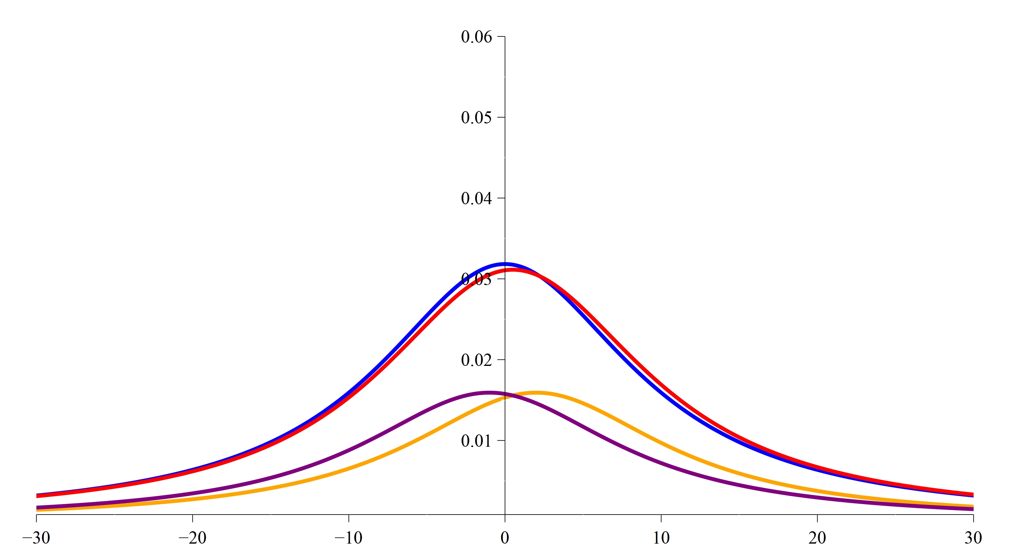
Figure 1: PDFs representing the prospects of the Null Option (blue) and the Basic Gamble (red), given a background prospect described by a Cauchy distribution with a location parameter of 0 and a scale parameter of 10. Purple and orange curves are ‘half PDFs’ representing the two possible outcomes of the Basic Gamble: They are obtained from the background distribution $\beta$ by multiplying by $0.5$ (representing the $0.5$ probabilities of each simple payoff), then translating by $+2$ and $-1$ respectively (representing the magnitudes of the simple payoffs). The prospect of the Basic Gamble is then obtained by summing the orange and purple curves. [Blue: $\beta_{N}(x)=\beta(x)=\left(10\pi(1+(\frac{x}{10})^{2})\right)^{-1}$. Purple: $\beta^{G}_{1}(x)=0.5\beta(x+1)$. Orange: $\beta^{G}_{2}(x)=0.5\beta(x-2)$. Red: $\beta_{G}(x)=\beta^{G}_{1}(x)+\beta^{G}_{2}(x)$.]

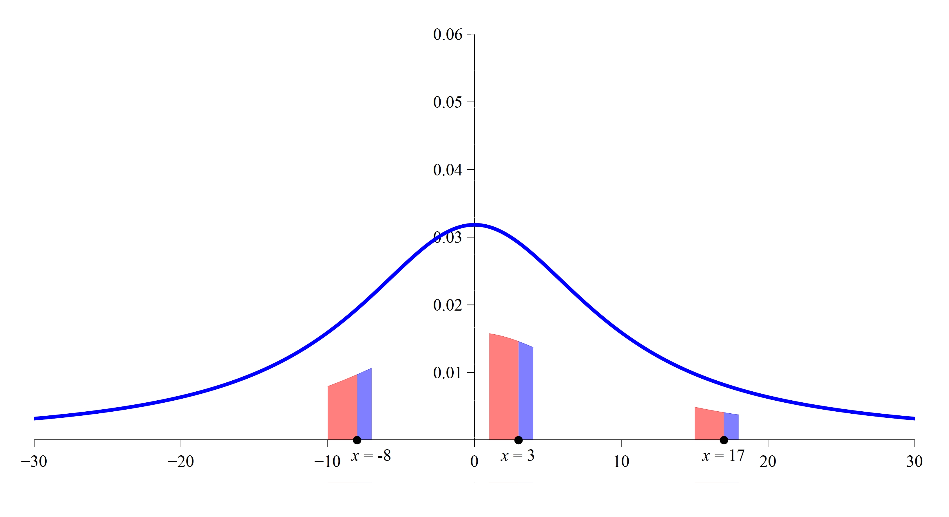
Figure 2: Red areas represent the joint probability of a simple payoff of $2$ and a background payoff in the interval $[x-2,x)$ (for $x=-8$, $3$, $17$). Blue areas represent the joint probability of a simple payoff of $-1$ and a background payoff in the interval $[x,x+1)$. $G$ stochastically dominates $N$ if for every $x$, $0.5\int_{x-2}^{x}\beta(y)\,dy$ (red) is greater than $0.5\int_{x}^{x+1}\beta(y)\,dy$ (blue).

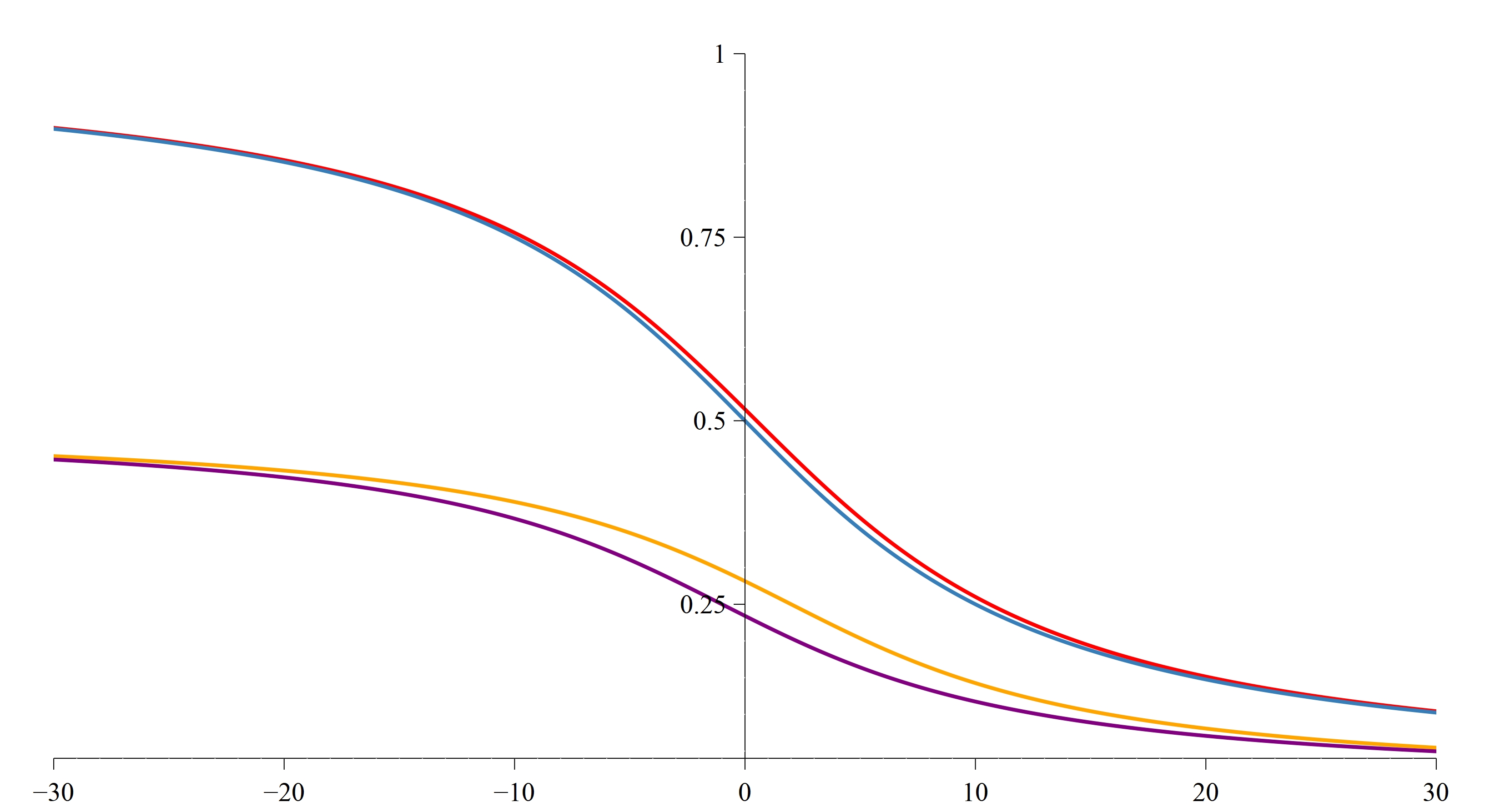
Figure 3: CCDFs (and ‘half CCDFs’) corresponding to the PDFs (and ‘half PDFs’) in Fig. 1. The blue curve gives the probability that the Null Option yields a payoff $\geq x$. The red curve gives the probability that the Basic Gamble yields a payoff $\geq x$. Purple and orange curves again represent the two possible simple payoffs of the gamble. $\bar{B}_{G}$ (red) is everywhere slightly greater than $\bar{B}_{N}$ (blue), indicating stochastic dominance. [Blue: $\bar{B}_{N}(x)=\bar{B}(x)=\frac{1}{\pi}\tan^{-1}\left(\frac{x}{10}\right)+0.5$. Purple: $\bar{B}^{G}_{1}(x)=0.5\bar{B}(x+1)$. Orange: $\bar{B}^{G}_{2}(x)=0.5\bar{B}(x-2)$. Red: $\bar{B}_{G}(x)=\bar{B}^{G}_{1}(x)+\bar{B}^{G}_{2}(x)$.]

Thus, $G$ offers a greater probability than $N$ of a payoff $\geq x$ iff $0.5\int_{x-2}^{x}\beta(y)\,dy>0.5\int_{x}^{x+1}\beta(y)\,dy$. If this inequality holds for every $x$, then $G$ stochastically dominates $N$ (see Fig. 2). Formally (and canceling the $0.5$’s):

$$\forall x\left(\int_{x-2}^{x}\beta\left(y\right)\,dy>\int_{x}^{x+1}\beta(y)\,dy\right)\Rightarrow G\succ_{sd}N$$

If $\beta$ is unimodal (i.e., strictly decreasing in either direction away from a central peak), then this condition will be trivially satisfied for values of $x$ in the right tail: Since $\beta$ is decreasing in the right tail, $\int_{x-2}^{x}\beta(y)\,dy$ will clearly be greater than $\int_{x}^{x+1}\beta(y)\,dy$, being both ‘wider’ and ‘taller’. The interesting question is whether it holds in the left tail. A sufficient condition for it to do so is that the value of $\beta$ never decreases by more than a factor of 2 in an interval of length 3: In this case, $\int_{x-2}^{x}\beta(y)\,dy$ is everywhere greater than $\int_{x}^{x+1}\beta(y)\,dy$, since it is twice as ‘wide’ (i.e., the interval $[x-2,x]$ is twice as long as the interval $[x,x+1]$) and everywhere at least half as ‘tall’ (i.e., the maximum value of $\beta$ on the interval $[x-2,x+1]$ is no more than twice the minimum value). This guarantees that by choosing $G$, at every point $x$ on the horizontal axis, you move more probability mass from the left of that point to the right (increasing the probability of a payoff $\geq x$) than from the right to the left (decreasing the probability of a payoff $\geq x$), which means that $G$ stochastically dominates $N$.

For $\beta$ to never decrease by more than a factor of 2 within an interval of length 3, it is sufficient that $\beta$ has large tails and a high enough dispersion. If a distribution has large tails, then for any finite $l$, there is some finite $r$ such that $\beta$ never decreases by more than a factor of $r$ within an interval of length $l$. And if for $l=3$ that factor is greater than 2, we can decrease it by ‘stretching’ $\beta$ (increasingly rescaling it), so that its tails decay more slowly.

The resulting stochastic dominance relation can be visualized by representing each prospect with its CCDF, as in Fig. 3: The Basic Gamble stochastically dominates the Null Option iff its CCDF is everywhere greater.

5.2 Sufficiency Theorem

We have now seen how background uncertainty can generate stochastic dominance. But how general is this phenomenon—does it depend on special and improbable conditions? In this section, we will partially answer that question by identifying a sufficient condition for $O_{i}$ to stochastically dominate $O_{j}$ under background uncertainty, that depends only on (i) a measure of the expectational superiority of $O_{i}$ to $O_{j}$ and (ii) the rate at which the tails of $\beta$ decay, relative to the range of possible simple payoffs from $O_{i}$ and $O_{j}$.

To state the result, we need some additional notation. First, we introduce a function that, for options $O_{i}$ and $O_{j}$, gives the difference between the probability that $O_{i}$ yields a simple payoff $\geq x$ and the probability that $O_{j}$ yields a simple payoff $\geq x$.

$$\Delta_{ij}(x):=\Pr(O_{i}\geq x)-\Pr(O_{j}\geq x)$$

$\Delta_{ij}$ can be understood as the difference of the CCDFs of the simple prospects of $O_{i}$ and $O_{j}$ (Fig. 4). We also define the positive and negative parts of $\Delta_{ij}$:

$$\Delta_{ij}^{+}(x):=\max(\Delta_{ij}(x),0)$$

$$\Delta_{ij}^{-}(x):=\max(-\Delta_{ij}(x),0)$$

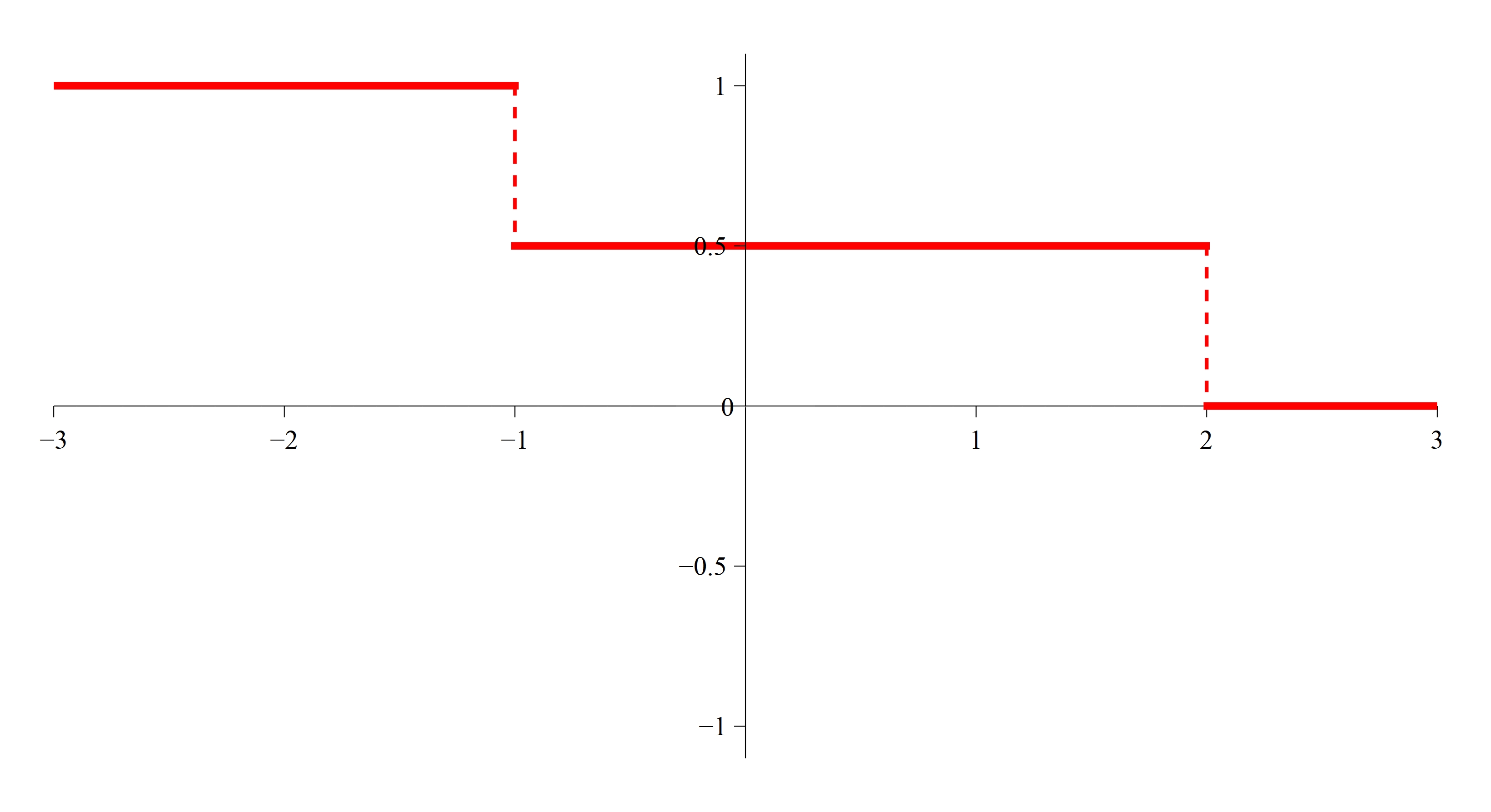
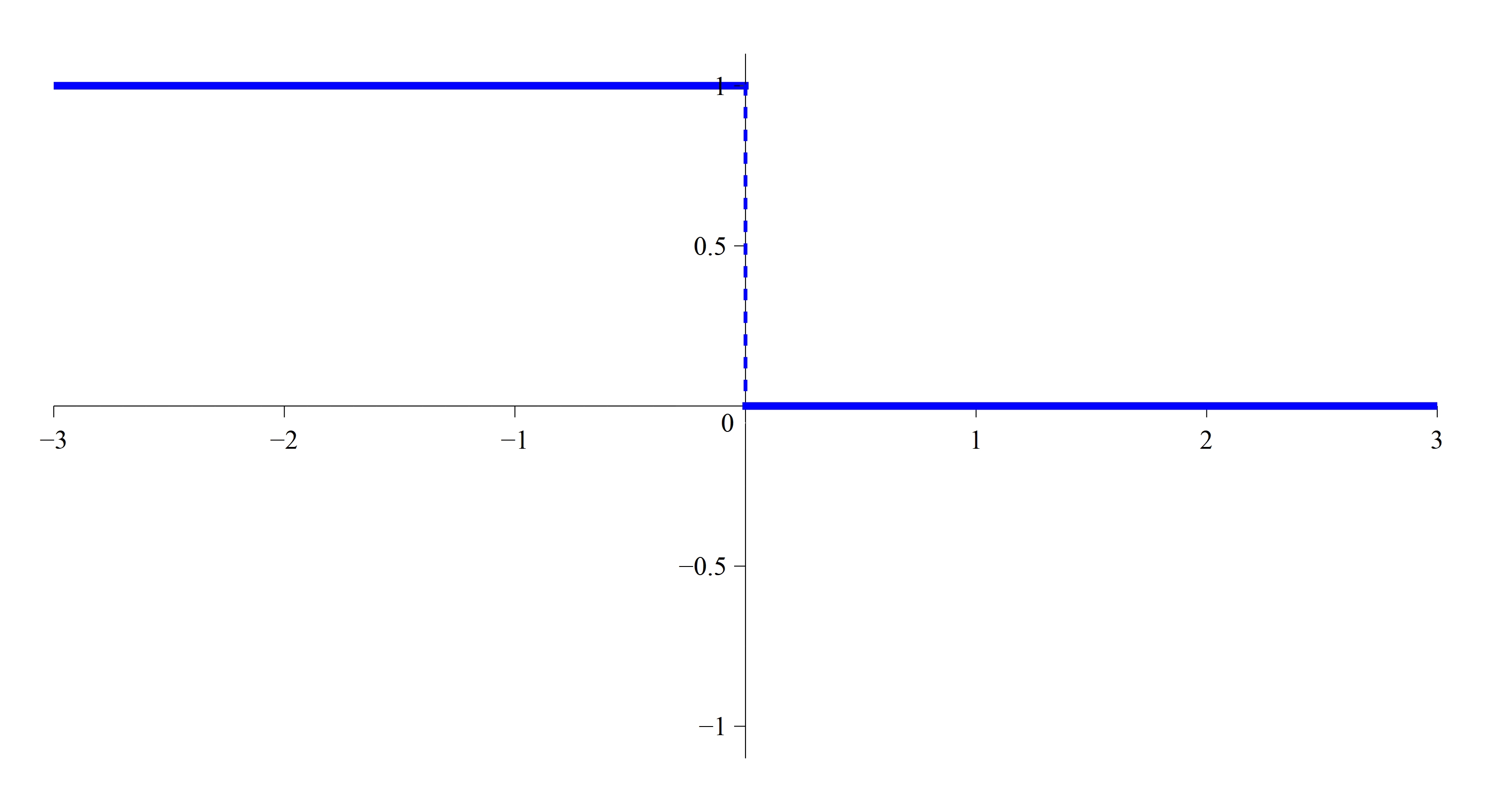
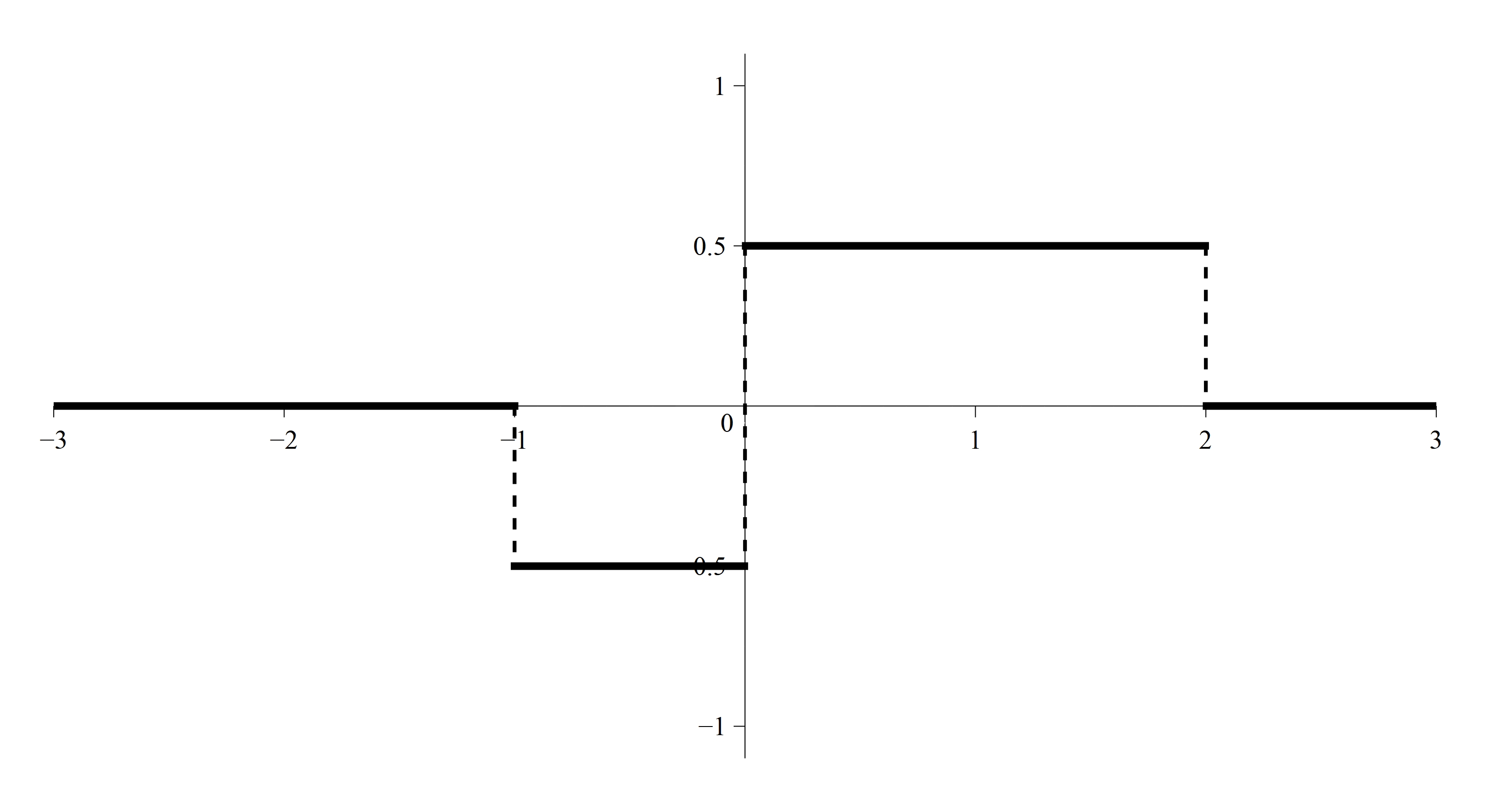
Figure 4: The CCDFs of the simple prospects of the Basic Gamble $G$ (left) and the Null Option $N$ (middle), and the difference $\Delta_{GN}$ of the two CCDFs (right).

The integral of $\Delta_{ij}$, $\int_{-\infty}^{\infty}\Delta_{ij}(x)\,dx=\int_{-\infty}^{\infty}\Delta_{ij}^{+}(x)\,dx-\int_{-\infty}^{\infty}\Delta_{ij}^{-}(x)\,dx$, gives the difference in expected choiceworthiness between $O_{i}$ and $O_{j}$. If $\Delta_{ij}$ is nowhere negative and somewhere positive, then $O_{i}$’s simple prospect stochastically dominates $O_{j}$’s, which guarantees that $O_{i}$ will stochastically dominate $O_{j}$ in any state of background uncertainty (Pomatto et al., 2020, p. 1880). On the other hand, if $O_{j}$’s simple prospect has a greater expectation than $O_{i}$’s, then it is impossible for $O_{i}$ to stochastically dominate $O_{j}$ in any state of background uncertainty (Pomatto et al., 2020, p. 1880). Thus, the cases of interest to us are those where $\Delta_{ij}$ is somewhere positive and somewhere negative, and where the integral of $\Delta_{ij}$ is positive.

Second, we introduce a function $\operatorname{rate}(O_{i},O_{j},\beta)$ that gives the maximum ratio between values of $\beta$ for arguments that differ by no more than the range of the support of $\Delta_{ij}$, denoted $|\operatorname{supp}(\Delta_{ij})|=\max(\operatorname{supp}(\Delta_{ij}))-\min(\operatorname{supp}(\Delta_{ij}))$. (In general, $|\operatorname{supp}(\Delta_{ij})|$ is the difference between the best and worst possible simple payoffs in $O_{i}$ and $O_{j}$.)

$$\operatorname{rate}(O_{i},O_{j},\beta):=\max_{x,y:|y|<|\operatorname{supp}(\Delta_{ij})|}\frac{\beta(x+y)}{\beta(x)}$$

This notation in hand, we can now state the first result.

Theorem 1 (Sufficiency Theorem).

For any options $O_{i}$, $O_{j}$ and background prospect $\beta$,

$$\frac{\int_{-\infty}^{\infty}\Delta_{ij}^{+}(x)\,dx}{\int_{-\infty}^{\infty}\Delta_{ij}^{-}(x)\,dx}>\operatorname{rate}(O_{i},O_{j},\beta)\Rightarrow O_{i}\succ_{sd}O_{j}.$$

The proof is given in the appendix. Intuitively, the theorem can be understood as follows: $\int_{-\infty}^{\infty}\Delta_{ij}^{+}(x)\,dx$ measures the ‘expectational upside’ of choosing $O_{i}$ over $O_{j}$, and $\int_{-\infty}^{\infty}\Delta_{ij}^{-}(x)\,dx$ measures the ‘expectational downside’, in the sense that the difference in expected choiceworthiness between $O_{i}$ and $O_{j}$ is given by $\int_{-\infty}^{\infty}\Delta_{ij}^{+}(x)\,dx-\int_{-\infty}^{\infty}\Delta_{ij}^{-}(x)\,dx$. The Sufficiency Theorem says that if the ratio of expectational upside to expectational downside is greater than the maximum amount by which the value of $\beta$ decays over an interval of length $|\operatorname{supp}(\Delta_{ij})|$ (roughly, the range of possible simple payoffs from $O_{i}$ and $O_{j}$), then $O_{i}$ stochastically dominates $O_{j}$.

If $\beta$ has large tails, then for any $O_{i}$, $O_{j}$, $\operatorname{rate}(O_{i},O_{j},\beta)$ will be finite. Moreover, if we ‘stretch’ $\beta$ along the $x$-axis (i.e., increasingly rescale it), $\operatorname{rate}(O_{i},O_{j},\beta)$ converges to 1. So if $\beta$ has large tails and $O_{i}$’s simple prospect is expectationally superior to $O_{j}$’s (so that $\frac{\int_{-\infty}^{\infty}\Delta_{ij}^{+}(x)\,dx}{\int_{-\infty}^{\infty}\Delta_{ij}^{-}(x)\,dx}>1$), $O_{i}$ will stochastically dominate $O_{j}$ given a sufficient rescaling of $\beta$. This means that, as we increasingly rescale $\beta$ (increasing its dispersion), the partial ordering of options by stochastic dominance, $\succ_{sd}$, asymptotically approaches the ordering of options by the expectations of their simple prospects.

5.3 Necessity Theorem

The Sufficiency Theorem also offers some suggestion that it is harder for background uncertainty to generate stochastic dominance in Pascalian contexts: All else being equal, increasing the range of simple payoffs increases $\operatorname{rate}(O_{i},O_{j},\beta)$, and so the condition $\frac{\int_{-\infty}^{\infty}\Delta_{ij}^{+}(x)\,dx}{\int_{-\infty}^{\infty}\Delta_{ij}^{-}(x)\,dx}>\operatorname{rate}(O_{i},O_{j},\beta)$ becomes more demanding. But since this is a sufficient rather than a necessary condition for stochastic dominance, this is only a suggestion.

The suggestion is confirmed, however, by the following necessary condition for stochastic dominance:

Theorem 2 (Necessity Theorem).

For any options $O_{i}$, $O_{j}$ and background prospect $\beta$,

$$O_{i}\succ_{sd}O_{j}\Rightarrow\max_{x}\Delta_{ij}(x)>\max_{x}\int_{-\infty}^{\infty}\Delta_{ij}^{-}(x-y)\beta(y)\,dy.$$

The proof is again left for the appendix. Intuitively, the theorem can be understood as follows: Choosing $O_{i}$ rather than $O_{j}$ changes the probability of an overall payoff $\geq x$ by $\int_{-\infty}^{\infty}\Delta_{ij}(x-y)\beta(y)\,dy$, which can be decomposed into positive and negative components, as $\int_{-\infty}^{\infty}\Delta_{ij}^{+}(x-y)\beta(y)\,dy-\int_{-\infty}^{\infty}\Delta_{ij}^{-}(x-y)\beta(y)\,dy$. Call $\int_{-\infty}^{\infty}\Delta_{ij}^{+}(x-y)\beta(y)\,dy$ the increment to the probability of a payoff $\geq x$ from choosing $O_{i}$ over $O_{j}$, and $\int_{-\infty}^{\infty}\Delta_{ij}^{-}(x-y)\beta(y)\,dy$ the decrement. The Necessity Theorem says that, for $O_{i}$ to stochastically dominate $O_{j}$, the maximum amount by which $O_{i}$ increases the probability of achieving a simple payoff $\geq x$, for any $x$ (given by $\max_{x}\Delta_{ij}(x)$), must exceed the maximum decrement to the probability of an overall payoff $\geq x$, for any $x$ (given by $\max_{x}\int_{-\infty}^{\infty}\Delta_{ij}^{-}(x-y)\beta(y)\,dy$).

This result tells us two things. First, whenever $O_{i}$’s simple prospect does not stochastically dominate $O_{j}$’s (so that $\max_{x}\int_{-\infty}^{\infty}\Delta_{ij}^{-}(x-y)\beta(y)\,dy$ is non-zero), there is some probability threshold such that sets of simple payoffs with total probability below that threshold cannot generate stochastic dominance, no matter their magnitude. To illustrate, suppose we make the choice between $O_{i}$ and $O_{j}$ more Pascalian by taking each positive simple payoff of $O_{i}$ and negative simple payoff of $O_{j}$, and replacing its simple payoff-probability pair with a smaller probability of a proportionately larger simple payoff, plus a complementary probability of a simple payoff of 0—that is, replacing $\langle v_{k},p_{k}\rangle$ with $\langle cv_{k},\frac{p_{k}}{c}\rangle,\langle 0,p_{k}-\frac{p_{k}}{c}\rangle$, for some constant $c$. This ‘Pascalian transformation’ preserves the expectations of both options. But as $c$ goes to infinity, $\max_{x}\Delta_{ij}(x)$ goes to 0, while $\max_{x}\int_{-\infty}^{\infty}\Delta_{ij}^{-}(x-y)\beta(y)\,dy$ does not, so $O_{i}$ must eventually cease to stochastically dominate $O_{j}$. More generally, holding other features of a choice situation fixed, SDTR will eventually cease to require the expectationally superior option as the source of its expectational superiority becomes increasingly Pascalian (reliant on very small probabilities of extreme simple payoffs).^,

But second, the probability threshold established by the Necessity Theorem—namely, $\max_{x}\int_{-\infty}^{\infty}\Delta_{ij}^{-}(x-y)\beta(y)\,dy$—is sensitive to the dispersion of $\beta$. As we increasingly rescale $\beta$ (increasing its dispersion without changing its shape), we spread its fixed budget of probability mass more thinly, so that $\max_{x}\int_{-\infty}^{\infty}\Delta_{ij}^{-}(x-y)\beta(y)\,dy$ must shrink, approaching zero in the limit. Thus, the greater the dispersion of $\beta$, the more Pascalian a choice situation can become while preserving stochastic dominance.

5.4 Illustrations and practical implications

The Sufficiency and Necessity Theorems give separate sufficient and necessary conditions for stochastic dominance. If we fill in some details, though, we can find necessary-and-sufficient conditions for stochastic dominance in restricted contexts. This lets us see just how tightly SDTR constrains risk attitudes in particular choice situations, both ‘ordinary’ and ‘Pascalian’.

First, let’s specify a background prospect: a Laplace distribution with a mean of zero and a scale parameter of $-\frac{500}{\ln(0.05)}$ ($\approx 166.9$). A Laplace distribution has exponential tails, and is therefore as light in the tails as any large-tailed distribution can be. The scale parameter of $-\frac{500}{\ln(0.05)}$ is chosen because it yields a 95% confidence interval of $[-500,+500]$, which gives an intuitive sense of the dispersion of the distribution. As we have implicitly done in previous examples, let’s assume that units represent lives saved/lost—or more precisely, the choiceworthiness of saving a typical happy human life (treating this, somewhat unrealistically, as a known quantity). We can abbreviate these units as life equivalents (LE). Our agent, then, is 95% confident that her background payoff will fall in an interval whose magnitude is 1000 LE (i.e., the value of 1000 human lives). For an agent who attaches normative weight to the total value of the world that results from her choices, this dispersion is implausibly small (as I will argue in §6.2). But I choose it in order to emphasize how easily background uncertainty can generate very strong stochastic dominance constraints on an agent’s choices.

To see the strength of these constraints, consider the following:

Generalized Basic Gamble (G^′) $\{\langle-1,0.5\rangle,\langle 0,0.5-p\rangle,\langle 2,p\in(0,0.5]\rangle\}$

We can interpret $G^{\prime}$ as an option that will save two lives with probability $p$, cause one death with probability $0.5$, and have no consequences with probability $0.5-p$.

$G^{\prime}$ has greater expected choiceworthiness than the Null Option $N$, of course, iff $p>0.25$. By comparison, and somewhat surprisingly, $G^{\prime}$ stochastically dominates $N$ iff $p>$ $\sim 0.25226$. So, even given a relatively light-tailed background prospect with modest dispersion, stochastic dominance imposes extremely tight constraints on the choice between $G^{\prime}$ and $N$—nearly as tight as those imposed by expectationalism.

This example illustrates the following more general point. If $\beta$ has large tails, then under various reasonable assumptions about its shape (e.g., that it belongs to a standard parameterized family of distributions like Laplace or Cauchy), SDTR will be tightly constraining (closely approximating the ranking of options by the expectations of their simple prospects) in any choice situation where the interquartile range of $\beta$ is significantly greater than the range of possible simple payoffs. Specifically, in these circumstances, $\operatorname{rate}(O_{i},O_{j},\beta)$ will be not much greater than 1, and thus the sufficient condition for stochastic dominance given by the Sufficiency Theorem will be relatively easily met. For instance, if $\beta$ is a Laplace distribution and its $\operatorname{IQR}$ is ten times greater than $|\operatorname{supp}(\Delta_{ij})|$ (which, remember, is less than or equal to the range of possible simple payoffs from $O_{i}$ and $O_{j}$), then $\operatorname{rate}(O_{i},O_{j},\beta)\approx 1.15$. For a Cauchy distribution, the equivalent figure is $\sim 1.22$. And as per the Sufficiency Theorem, it is sufficient (though not necessary) for stochastic dominance that $\frac{\int_{-\infty}^{\infty}\Delta_{ij}^{+}(x)\,dx}{\int_{-\infty}^{\infty}\Delta_{ij}^{-}(x)\,dx}$ (the ratio of ‘expectational upside’ to ‘expectational downside’ from choosing $O_{i}$ over $O_{j}$) exceeds this threshold.

By contrast, consider the following ‘Pascalian transformation’ of $G^{\prime}$:

Generalized Pascalian Gamble (G^′′) $\{\langle-1,0.5\rangle,\langle 0,0.5-p\rangle,\langle 2000,p\in(0,0.0005]\rangle\}$

$G^{\prime\prime}$ has greater expected choiceworthiness than $N$ iff $p>0.00025$. But in this case, $G^{\prime\prime}$ only comes to stochastically dominate $N$ when $p>$ $\sim 0.0030047$—more than ten times the probability at which $G^{\prime\prime}$ becomes expectationally superior. This illustrates the difference between the tight constraints imposed by stochastic dominance in cases involving intermediate probabilities of modest simple payoffs, and the relative latitude it allows in cases involving very small probabilities of very large simple payoffs.

What does this mean for potentially Pascalian choices in the real world—e.g., choosing between interventions that do moderate amounts of good with high probability in the near term and interventions that try to influence the far future, doing potentially astronomical good, but with (plausibly) very low probability of success? Fully answering this question is a large project unto itself (requiring, among other things, a plausible model of our actual background uncertainty and of the probabilities and payoffs involved in the interventions we wish to compare). But as a first approximation, let’s consider another stylized case in which we must choose between a ‘sure thing’ option that saves some small number of lives $s$ for certain ($S=\{\langle s,1\rangle\})$ and an expectationally superior ‘long shot’ option that tries to prevent existential catastrophe, thereby enabling the existence of astronomically many future lives, but has only a very small probability of making any difference at all ($L=\{\langle 0,1-p\rangle,\langle a,p\rangle\}$, where $a$ is astronomically large, $p$ is very small, and $ap>s$). And let’s assume of the agent’s background prospect only that it has large tails and that its dispersion (as measured by interquartile range) is several orders of magnitude greater than the sure-thing payoff $s$.

First, the Necessity Theorem implies that there is a minimum value of $p$ below which $L$ cannot stochastically dominate $S$, no matter the magnitude of $a$. It turns out that this threshold can be fairly well approximated by $\frac{s}{\operatorname{IQR}(\beta)}$, the ratio of the sure-thing payoff to the interquartile range of the background prospect. So for instance, if $s=10$ LE and $\operatorname{IQR}(\beta)=10^{9}$ LE, then the ‘Pascalian threshold’ for values of $p$ below which $L$ cannot stochastically dominate $S$ will likely be in the neighborhood of $10^{-8}$ (with its exact value depending on the shape of $\beta$).

This threshold applies to $L$ no matter the magnitude of the astronomical simple payoff $a$. How much do things change if we consider some particular value of $a$, like Bostrom’s $10^{52}$ LE? The short answer is: not much. For these purposes, payoffs that are very large relative to the dispersion of the background prospect can, to a very close approximation, be treated as infinite. Thus, if $a=10^{52}$ LE and $\operatorname{IQR}(\beta)\ll 10^{52}$ LE, the threshold at which $L$ stochastically dominates $S$ will be roughly $\frac{s}{\operatorname{IQR}(\beta)}$.

This suggests a strategy for proponents of Bostrom-style arguments (and ‘longtermists’ more generally) to allay concerns about Pascalian fanaticism. Suppose you have some limited resource, like money, that you can use either to do some definite short-term good or to slightly increase the probability of a positive long-term trajectory for humanity. And suppose we know the latter option to be expectationally superior, despite its small probability of impact. If the amount by which a marginal unit of resource can increase the probability of a positive long-term trajectory exceeds the ratio between the amount of good you could do by spending that same unit of resource on short-term causes and the interquartile range of your background prospect, then very plausibly the longtermist option will turn out to be stochastically dominant, in which case we should have no decision-theoretic reservations about favoring it. For instance, suppose you can either save 100 lives for sure or reduce the probability of existential catastrophe by $10^{-9}$, thereby potentially enabling $10^{52}$ future lives. If the interquartile range of your background prospect is significantly greater than $10^{11}$ LE, then the longtermist option is likely to be stochastically dominant. And if your background uncertainty reflects uncertainty about the total amount of value in the Universe, it seems quite plausible—though perhaps not indisputable—that its dispersion should be at least this great. (We will consider this question in §6.2.) But if, on the other hand, you can only have a much smaller effect on the probability of existential catastrophe (say, $10^{-30}$), then much greater background uncertainty will be needed for stochastic dominance, and even though the expectations may still be astronomical (in this case, $10^{22}$ LE), it looks more plausible that you are rationally permitted to prefer the expectationally inferior ‘sure thing’.

In light of the preceding discussion, it seems to me that the greatest intuitive worry about SDTR in the presence of large-tailed background uncertainty is not that it will capture too little of expectational reasoning (failing to recover intuitive constraints on our choices), but rather that it will capture too much—requiring us to accept many gambles that seem intuitively Pascalian (e.g., where the probability of any positive payoff is on the order of $10^{-9}$ or less). But really, this is not a worry at all: Unlike primitive expectationalism, SDR is supported by a priori arguments far more epistemically powerful than our intuitions about Pascalian gambles. If some gambles that seem intuitively Pascalian turn out to be stochastically dominant once we account for our background uncertainty, we should not conclude that stochastic dominance is implausibly strong. Rather, we should conclude that there is a much more compelling argument for choosing the expectation-maximizing option in these cases than we had previously realized. This would be not a reductio but rather an unexpected and practically important discovery.

6 Sources of background uncertainty

The results above are practically significant only if some agents are (or ought to be) in a state of background uncertainty with large tails and at least moderate dispersion. In this section, I argue that this sort of background uncertainty is rationally required, at least for many agents, in real-world choice situations. In §§6.1–6.2, I argue that large tails and high dispersion respectively are appropriate for aggregative consequentialists. In §6.3, I generalize these arguments to agents who accept ‘mixed’ theories, giving weight to overall consequences but also to other kinds of normative considerations. In §6.4, I argue that the preceding conclusions at least partly generalize to ‘parochial’ agents who give no weight at all to the value of the world as a whole, caring only about some narrow circle of moral concern like their family, village, or nation.

6.1 Large tails

In this subsection, I give three arguments that our uncertainty about the total amount of value in the world has large tails, and therefore that aggregative consequentialists at least should be in a state of large-tailed background uncertainty.

First, an intuitive argument: The ‘large tails’ condition is in fact very modest. Setting aside some contrived exceptions, a distribution has large tails as long as there is some finite upper bound on the ratios of probabilities assigned to adjacent intervals of a fixed length, like $[x-1,x]$ and $[x,x+1]$. In our context, this means there is an upper bound on how much more probable I take it to be that the Universe contains between $x-1$ and $x$ units of value than that it contains between $x$ and $x+1$ units of value (or vice versa). The only way there could fail to be such a bound (given that $\beta$ is supported everywhere) is if the ratio of probabilities assigned to adjacent intervals increased without bound in one or both tails of $\beta$. But this implies that I become arbitrarily confident about the relative probability of very similar hypotheses, in a domain where I seem to have virtually no grounds for such discrimination. It would mean, for instance, that I find it vastly more probable that the Universe contains between $-18,946,867,974,834$ and $-18,946,867,974,835$ units of value than that it contains between $-18,946,867,974,835$ and $-18,946,867,974,836$ units of value. And as the numbers get larger, my relative confidence only gets (boundlessly) greater. But it seems obvious that, if anything, the degree to which I discriminate between such adjacent hypotheses should diminish in the extreme tails of $\beta$. None of my evidence provides any serious support for the first of the above hypotheses ($[-...5,-...4]$) over the second ($[-...6,-...5]$), at least not in any way that I am capable of identifying.

The second argument is more concrete: Attempting to model our actual background uncertainty, even on fairly conservative assumptions, yields tails significantly heavier than exponential.

Assume that welfare is one of the things that contributes to the total amount of value in the Universe. Then, unless other normative considerations are systematically anti-correlated with welfare, our background uncertainty should be at least as great as our uncertainty about total welfare. This uncertainty derives from uncertainty about both (i) the number of welfare subjects in the Universe and (ii) their average welfare. Either of these factors could give us large tails, but (i) is the most straightforward.

Our uncertainty about the size of the Universe provides a useful lower bound on our uncertainty about the total number of welfare subjects. There is no known upper bound on the size of the Universe as a whole, which we know must be many times larger than the observable universe. There is therefore no known upper bound on the number of welfare subjects in the Universe. Actually quantifying our uncertainty about the size of the Universe requires a choice of prior, which is of course a fraught endeavor whose philosophical difficulties we will not be able to resolve here. But the best we can do is to choose a reasonable and conservative prior and see where it leads us. Vardanyan et al. (2009) suggest a physically motivated prior that they call the astronomer’s prior. Conditional on a finite universe, the astronomer’s prior is uniform over values of $\Omega_{k}$ in the interval $(0,1]$, where $\Omega_{k}$ is the curvature parameter in the standard $\Lambda$CDM cosmology (smaller values of $\Omega_{k}$ indicating less curvature and hence a larger Universe). This implies a prior over the present curvature radius of the Universe, $a_{0}$, where $\Pr(a_{0})\propto a_{0}^{-3}$, which in turn implies a prior over the present volume of the Universe, $V$, where $\Pr(V)\propto V^{-\frac{5}{3}}$. And this distribution is extremely heavy-tailed—much heavier than exponential.

Given such a heavy-tailed distribution for the size of the Universe, a large-tailed distribution for total welfare in the Universe (or, in the part of the Universe unaffected by our choices) is nearly a foregone conclusion, requiring only (i) that the number of welfare subjects per unit of comoving spatial volume is not strongly anti-correlated with the size of the Universe and (ii) that we assign non-zero probability to both positive and negative values for the average welfare of all welfare subjects. The second assumption looks unassailable, and I cannot think of a reason to question the first.

The most serious objection I can see to the preceding line of argument is that the Universe, and the number of welfare subjects it contains, may well be infinite (Knobe et al., 2006; Vardanyan et al., 2009; Carroll, 2017). I will, unfortunately, have little to say about this issue (though I say a bit in §9.6 below). I take it for granted that the true axiology can make non-trivial comparisons between infinite worlds, so that even if we were certain that the Universe was infinite, we could still be uncertain about its overall value. But how (if at all) we extend the arguments of this paper to the infinite context depends very much on what sort of infinite axiology we adopt, and there is as yet no agreement even on very basic questions about how to formulate an infinite axiology. Perhaps more to the point (though no more satisfying), expectational reasoning is if anything more threatened by infinite worlds than stochastic dominance reasoning (see for instance Bostrom (2011, pp. 13ff), Arntzenius (2014)). So even if the arguments in this paper suffer in an infinitary context, that is not likely to generate much support for expectationalism over SDTR.

The third and final argument for large tails is the simplest: When I am uncertain which of several probability distributions best characterizes some phenomenon, the resulting mixture distribution (the probability-weighted average of the distributions over which I’m uncertain) inherits the tail properties of the heaviest-tailed distribution in the mixture. (The further out we go in the tails of the mixture distribution, the more the heaviest-tailed distributions dominate the mixture.) So, suppose I am unsure what background prospect is justified by my evidence, or that I assign credence to multiple physical theories that imply different objective probability distributions over background payoffs. As long as I assign positive credence to any distribution with exponential or heavier tails, the resulting background prospect will have exponential or heavier tails. And, excluding some contrived and unlikely cases, a background prospect with exponential or heavier tails (i.e., that is bounded below in the tails by a Laplace distribution) will also satisfy our ‘large tails’ condition.

6.2 High dispersion

Large tails create the conditions for background uncertainty to generate stochastic dominance, but as we saw in §5, how closely stochastic dominance approximates the ordering of options by the expectations of their simple prospects depends on the dispersion of the background prospect—intuitively, how ‘spread out’ it is. A distribution can have very heavy tails while nevertheless having arbitrarily low dispersion, concentrating most of its probability mass in a very small interval.

As we saw in §5.4, SDTR is generally tightly constraining when $\beta$ has large tails and a dispersion that is large relative to the range of possible simple payoffs. For SDTR to yield intuitively satisfactory constraints in real-world choice situations, then, it should be the case that the dispersion of our real-world background uncertainty is large relative to the stakes we face in most real-world choice situations. If our background uncertainty reflects our uncertainty about the total amount of value in the Universe, this ‘high dispersion’ premise strikes me as nearly indisputable, and less in need of defense than the ‘large tails’ premise. So I will just briefly note three arguments for high dispersion.

First, the population of welfare subjects on Earth up to the present is both very large and a matter of great uncertainty. And we can say very little about average welfare in this historical population, including whether it has been positive or negative. Hence our uncertainty about total welfare on Earth up to the present moment (one contributor to our background uncertainty) has very high dispersion.

Second, we saw above that our uncertainty about the size of the Universe as a whole is very great (Vardanyan et al., 2009, 2011), as is our uncertainty about the number of inhabited planets and hence the number of welfare subjects per unit of spatial volume (Sandberg et al., 2018). And here too, even more so than in the terrestrial case, we know next to nothing about average welfare. So our uncertainty about the total welfare of non-Earth-originating welfare subjects outside our future light cone (another contributor to our background uncertainty) also has very high dispersion.

Finally, it is worth mentioning a third source of background uncertainty: an agent’s uncertainty about the outcomes of other future choices (and perhaps some past choices as well), both her own and those of other agents. When those choices, and their outcomes, are suitably independent of the agent’s present choice, they can be treated as part of her background uncertainty. Simplifying considerably, if an agent believes that future agents (herself perhaps included) will face $n$ choices roughly similar to her own present choice, and that these choices and their outcomes are all suitably independent, then her background uncertainty about the cumulative outcome of all those future choices will be her uncertainty about the outcome of an $n$-step independent random walk, with dispersion proportionate to $\sqrt{n}$. Assuming, then, that the choice our agent faces is ‘ordinary’ enough that she expects many similar choices to be faced by future agents, her uncertainty about the cumulative outcome of these future choices (a third contributor to her background uncertainty) is likely to have a dispersion that is large relative to the possible simple payoffs of her present options.

To stake out a definite, quantitative conclusion: Based on the preceding arguments, it seems clear to me that the dispersion (as measured by $\operatorname{IQR}$) of our background uncertainty about the total amount of value in the Universe must be at least on the order of $10^{9}$ LE, and perhaps very much larger.

6.3 ‘Mixed’ normative theories

We have thus far focused on agents who are exclusively concerned with aggregative consequentialist considerations, i.e., who measure the choiceworthiness of their options entirely by the total amount of value in the resulting world. But I think that the results in §5 are much more widely applicable. Unfortunately, I don’t see any way of establishing this except to consider, case by case, the various kinds of normative theory that an agent might use to gauge the choiceworthiness of her options. And doing this at all comprehensively would be a long and tedious exercise. So for now, I will simply point out two ways in which the phenomenon of large-tailed background uncertainty with high dispersion, and hence the practical significance of the results in §5, generalizes beyond aggregative consequentialism.

First, consider an agent who accepts a ‘mixed’ theory, measuring the choiceworthiness of her options partly by the total amount of value in the resulting world, but also by various other considerations, like whether she is keeping her promises, being a good friend, or exhibiting virtues like temperance and modesty, and perhaps giving extra weight to her own welfare/life projects, beyond their contribution to the overall value of the world. For simplicity, suppose she treats all these considerations as making additively separable contributions to the choiceworthiness of her options. And suppose that all of the non-aggregative-consequentialist considerations are captured by the simple payoffs of her options, so that her background uncertainty still reflects only uncertainty about the total amount of value in the Universe. (These are significant assumptions, though I cannot see any particular way in which plausibly weakening them would derail the conclusions below.) Then, of course, all the arguments for large tails from §6.1 will still apply. And the dispersion of $\beta$ will still typically be large relative to the range of simple payoffs, so long as it is large relative to the weight the agent attaches to ordinary non-consequentialist considerations. Suppose, for instance, that $\operatorname{IQR}(\beta)=10^{9}$ LE, which I suggested above as a conservative lower bound on our uncertainty about the total amount of value in the Universe. Only the most extreme deontological views assign ordinary non-consequentialist considerations a weight anywhere near that order of magnitude. So this agent will still, at least in most choice situations, find that the dispersion of her background prospect is much larger than the possible simple payoffs of her options, and hence that her choices are fairly tightly constrained by stochastic dominance.

6.4 ‘Parochial’ normative theories

Next, consider an agent whose concerns are ‘parochial’—i.e., not with the value of the Universe as a whole, but circumscribed within some fairly narrow ‘moral circle’. At the most extreme, such an agent might assign normative significance only to her own welfare. Alternatively, she might assign significance only to the welfare of her family, her tribe, local community, or nation, the present generation, the human species, or Earth-originating life, while ignoring all other sources of value in the Universe.

First, should such an agent’s background prospect have large tails? A prior question is, should it even be unbounded, or can an agent who cares only about, say, her own village be certain that its total welfare will not exceed some finite upper/lower bounds? I am inclined to say that, however narrow an agent’s moral circle, her background prospect must be unbounded, on the grounds that we should assign probability zero only to a priori impossibilities and, perhaps, to propositions that have been directly contradicted by observation. But this view is of course controversial, and I won’t try to defend it here. Assuming that a parochial agent’s background prospect should still be unbounded, however, the first and third arguments for large tails in §6.1 still seem to apply: Thinner tails would require the agent to have enormous relative confidence about very similar hypotheses that her evidence does little if anything to distinguish. And higher-level uncertainty will result in a heavy-tailed mixture distribution as her background prospect.

But what about dispersion? Certainly an agent who cares only about (say) her village will have a lower-dispersion background prospect than one who cares impartially about all welfare subjects in the Universe. Nevertheless, it seems plausible that even she will find that the dispersion of her background prospect is large relative to the possible simple payoffs of her options in most ordinary choice situations. Even my uncertainty about my own lifetime welfare, excluding the outcome of my present choice, is quite large (i.e., high-dispersion) relative to the stakes I face in most ordinary choice situations. And all the more so for my uncertainty about the welfare of my family, community, or nation. Finally, the third argument for high dispersion in §6.2 seems fairly general: As long as there are many similar choices with unknown and independent effects on the things I care about, the dispersion of my uncertainty about their cumulative outcome is likely to be large relative to the stakes of my present choice.

7 The rational significance of background uncertainty

An initially counterintuitive feature of the preceding arguments is their implication that what an agent rationally ought to do can depend on her uncertainties about seemingly irrelevant features of the world. To put the point as sharply as possible: Whether I am rationally required, for instance, to take a risky action in a life-or-death situation can depend on my uncertainties about the existence, number, and welfare of sentient beings in distant galaxies, perhaps outside the observable universe, with whom I will never and can never interact, on whom my choices have no effect, and whose existence, number, welfare, etc, make no difference to the local effects of my choices.

Surprising and counterintuitive though this conclusion may seem, however, I think it is fully intelligible on reflection. In this section, I will try to dispel (or at least mitigate) the feeling of counterintuitiveness. To do that, I will first describe a simple case where the rational relevance of background uncertainty is intuitively clear, then argue that what is true of this simple case is true of more complex cases as well.

Here, then, is the simple case:

Methuselah’s Choice

Methuselah is, and knows himself to be, the only sentient being in the Universe (past, present, or future). He came into existence finitely long ago, and has so far been in a neutral state. He now faces a choice—the only choice he will ever make. He can choose either $O_{1}$, which yields 100 years of happy life for sure, or $O_{2}$, which yields 1500 years of happy life with probability $0.1$, or zero years of happy life with probability $0.9$.

If these years of happy life are the only potential source of value in the Universe, it seems intuitively obvious to me that Methuselah is rationally permitted to make either choice. Even if he is rationally required to satisfy the VNM axioms, say, these alone do not tell him which option to choose. And long-run arguments for expectationalism are irrelevant as well, since Methuselah knows for certain that there is no long run.

But now suppose that we add a source of background uncertainty:

Methuselah’s Box

In addition to Methuselah, Methuselah’s universe contains a magic box, which contains a random number generator. After Methuselah makes his choice between $O_{1}$ and $O_{2}$, the box will generate a real number, from a Laplace distribution centered at zero with a scale parameter of 10,000, and open itself to reveal that number to Methuselah. In addition to the simple payoff from his choice, Methuselah will receive a number of happy life-years equal to the number generated by the box (if it is positive) or a number of unhappy life-years equal to the absolute value of that number (if it is negative).

(To avoid comparisons between happy and unhappy life-years, assume that whatever total payoff Methuselah receives, it will come in the form of exclusively happy or exclusively unhappy life-years. Thus, for instance, if he receives $+1500$ from his choice and $-2000$ from his box, he will experience 500 years of unhappy life. If he gets $+1500$ from his choice and $-200$ from his box, he will experience 1300 years of happy life.)

In virtue of Methuselah’s uncertainty about the background payoff he will receive from his box, $O_{2}$ now stochastically dominates $O_{1}$ (assuming only that Methuselah regards happy life as better than unhappy life, more happy life as better, and more unhappy life as worse). And for precisely this reason, it now seems clear that Methuselah rationally ought to choose $O_{2}$. Absent the uncertainty that his box introduces, Methuselah could have reasoned his way to choosing $O_{1}$ on the grounds that if he chooses $O_{1}$, he will certainly receive at least 100 years of happy life, while if he choose $O_{2}$, he very probably will not. And there is no compelling defeater to this reasoning, provided that (as I claimed above) there is no compelling argument in this case for risk-neutrally maximizing expected happy life-years. But once we introduce the box, there is a compelling defeater to the original justification for $O_{1}$. First, Methuselah is not guaranteed to experience at least 100 years of happy life if he chooses $O_{1}$. Second, in fact, he has a better chance of experiencing at least 100 years of happy life if he chooses $O_{2}$. And third, the same is true for any other possible payoff: Whatever payoff he chooses to focus on, Methuselah has a better chance of a payoff at least that good if he choose $O_{2}$. Thus, Methuselah’s background uncertainty gives him conclusive grounds for choosing $O_{2}$.

The lesson of Methuselah’s case generalizes straightforwardly to more ordinary choice situations. Suppose that Alice is a total hedonistic utilitarian and faces a choice between $O_{1}$, which will do an amount of good equivalent to 100 happy life-years with probability $1$, and $O_{2}$, which will do an amount of good equivalent to 1500 happy life-years with probability $0.1$, and do nothing with probability $0.9$. Suppose that Alice’s beliefs about total welfare in the Universe, apart from the effects of her present choice, are described by a Laplace distribution centered at zero with a scale parameter of 10,000 happy-life-year-equivalents. Alice’s situation is in every relevant respect equivalent to Methuselah’s: It makes no difference, from a utilitarian standpoint, whether the welfare at stake is the agent’s own, whether it belongs to a single welfare subject or to many, whether those subjects are near to the agent in space or time, etc. Just as in the case of Methuselah, therefore, we should conclude that (i) if there were nothing of moral significance in the Universe apart from the simple payoff of $O_{1}$ or $O_{2}$, then there would be no decisive justification for choosing $O_{2}$, but (ii) Alice’s background uncertainty, by making $O_{2}$ stochastically dominant over $O_{1}$, gives her just such a decisive justification.

Does this reasoning apply only to rigorously orthodox utilitarians like Alice, who are committed to universal impartiality and the interpersonal fungibility of welfare? No. All it really depends on is the fungibility of choiceworthiness, which is a conceptual truth so trivial it is hardly worth stating. Suppose that Bob accepts a commonsense, pluralistic theory of practical reasons, faces a choice between $O_{1}$ and $O_{2}$, where $O_{1}$ has a simple prospect of $\{\langle 100,1\rangle\}$, $O_{2}$ has a simple prospect of $\{\langle 0,0.9\rangle,\langle 1500,0.1\rangle\}$, and his background uncertainty is Laplacian with a scale parameter of 10,000. Then for any degree of choiceworthiness, $O_{2}$ gives Bob a better chance of performing an action at least that choiceworthy, which provides a uniquely decisive justification for choosing $O_{2}$. The contributors to choiceworthiness may be more complex and heterogeneous in Bob’s case than in Methuselah’s. But this merely obscures, and does not undermine, the simple argument for avoiding stochastically dominated options. From the standpoint of rational choice, Bob’s case is no different from Methuselah’s.

8 Two modest conclusions

What decision-theoretic conclusions should we take away from the preceding arguments? In this section, I describe two relatively moderate conclusions we might draw. In the next section, I make the case for my own more ambitious conclusion.

8.1 A decision theory for consequentialists?

In recent years, there has been much activity at the intersection of ethics and decision theory, and considerable interest in the idea of ‘ethical decision theory’—a decision theory distinct from expected utility theory that either governs ethical decision-making in general or serves as the decision-theoretic component of particular ethical theories. Along these lines, the results in §5 might be seen as laying the foundation for a ‘utilitarian decision theory’, analogous to recent attempts to develop a ‘deontological decision theory’ (Colyvan et al., 2010; Isaacs, 2014; Lazar, 2017). Though I have argued that the significance of these results generalizes well beyond purely consequentialist theories like classical utilitarianism, their significance is most clear and straightforward in that context. For instance, the additive separability of simple and background payoffs is trivial for classical utilitarians, and as we saw in §6, uncertainty about total welfare in the Universe provides an especially strong source of background uncertainty. We might conclude from the preceding arguments, then, that SDTR is an attractive ethical decision theory for classical utilitarians and other aggregative consequentialists.

At a minimum, though, we have found that accounting for background uncertainty gives aggregative consequentialists a new and powerful basis for choosing options whose simple prospects maximize expected objective value (and not just the expectation of some increasing function of objective value) in most ordinary choice situations—even if they are also subject to decision-theoretic requirements besides stochastic dominance. That is, we have reached an important practical conclusion for aggregative consequentialists that requires no decision-theoretic assumptions besides the almost entirely uncontroversial SDR. A fortiori, this conclusion applies to any aggregative consequentialist who satisfies any of the standard axiom systems like VNM or Savage, or even non-standard axiom systems like that of Buchak’s (2013) REU (which, like VNM and Savage, satisfies stochastic dominance). Any such agent must, in practice, rank options almost exactly by the expectations of their simple prospects, even if she is extremely risk-averse or risk-seeking with respect to objective value (except in Pascalian situations where, as we have seen, she may enjoy greater latitude).

8.2 An add-on to standard decision theory?

Building on the last observation, we can understand the results in §5 as providing a friendly ‘add-on’ to axiomatic expectationalism: Under sufficient background uncertainty, the standard axioms (via SDR) impose strict constraints on an agent’s ranking of simple prospects, constraints that don’t follow from those axioms in the absence of background uncertainty. Specifically, agents can be rationally required to rank options in a way that closely approximates the expectational ranking of their simple prospects under a particular, privileged assignment of cardinal values to payoffs—namely, the assignment that satisfies additive separability between simple and background payoffs.

Plausibly, this privileged cardinalization will match the natural cardinal structure of the phenomena in the world to which the agent attaches normative weight. For instance, suppose that I only care about my lifetime income, always preferring more income to less. The only assignments of cardinal values to outcomes that allow additive separability between simple payoffs (the monetary reward of my present choice) and background payoffs (the remainder of my lifetime income) will be those that are positive affine transformations of the monetary value of payoffs, as measured in a currency like dollars or euros. So under sufficient background uncertainty, SDR and any axiomatic theory that implies it will require me to rank my options approximately by the expected monetary value of their simple prospects.

To put the point a little differently: Under sufficient background uncertainty, the standard axioms (by way of SDR) let us derive strong decision-theoretic conclusions merely from the agent’s ranking of payoffs, without any information about her ranking of uncertain prospects. The add-on to standard decision theory here is not SDR, which was already implied, but rather the idea that agents often are or ought to be in a state of large-tailed background uncertainty. Recognizing this sort of background uncertainty does not impose any new constraints on the agent’s utility function per se: Given a ranking of overall payoffs, she may still maximize the expectation of any utility function that is increasing with respect to that ranking. But background uncertainty forces all these utility functions to agree much more than they otherwise would on the ranking of options, in a way that makes it look as if the agent was simply maximizing her expected simple payoff on a privileged cardinal scale.

As promised in §2, I haven’t given any novel arguments for rejecting any of the standard axioms of expected utility theory, except to show that we can derive strong and intuitively attractive practical conclusions about choices under uncertainty without appeal to those axioms. If you are inclined to accept the standard axioms, then, it is natural to adopt this ‘add-on’ interpretation of the preceding arguments, as supplementing rather than supplanting axiomatic expectationalism.

9 Stochastic dominance as the criterion of rational choice

But I will defend a more ambitious conclusion: that SDTR rather than expectationalism is the correct theory of rational choice under uncertainty. Or at least, I will argue that this view deserves consideration. My argument, in short, in this: The major disadvantage of SDTR relative to expectationalism is its apparent failure to place plausible constraints on our risk attitudes. On the other hand, SDTR has a number of advantages over expectationalism, some of which we’ve already seen and others of which will be described in this section. These advantages are significant enough that, if SDTR can in fact recover intuitively satisfactory constraints on our risk attitudes in real-world choice situations, then it deserves to be seen as a serious competitor to expectationalism.

We have already seen two possible advantages of SDTR. First, its requirements rest on stronger a priori foundations than those of expectationalism. Second, unlike primitive expectationalism, it can constrain our risk attitudes in ordinary situations while avoiding fanaticism in Pascalian situations (without recourse to ad hoc devices like excluding ‘de minimis probabilities’). In this section, I will briefly survey some other cases where SDTR outperforms primitive and/or axiomatic expectationalism. Some of these are still problem cases for SDTR, where it is not obvious what stochastic dominance reasoning will imply or where it gives less guidance than we would like. But in all of them, SDTR delivers better answers than expectationalism seems capable of providing.

In this survey, I will mainly ignore the effects of background uncertainty. Describing those effects in each of the problem cases discussed below is (at least) a paper unto itself, and my aim is only to illustrate that there is a broad range of cases in which SDTR outperforms expectationalism.

9.1 Infinite payoffs

The simplest problem cases for expectational decision theory are those involving possibilities of infinite positive and/or negative payoffs, as exemplified by Pascal’s Wager (Pascal, 1669). In these cases, expectational reasoning delivers either implausible advice or no advice at all. On the other hand, even in the absence of background uncertainty, stochastic dominance can often deliver plausible verdicts. To illustrate, let’s consider a few variants of the Wager.

Case 1: Pascal’s Wager (Costly)

• $\{\langle 10,1\rangle\}$

• $\{\langle 9,0.99\rangle,\langle+\infty,0.01\rangle\}$

Here, expectationalism implies that $O_{2}$ is rationally required, while SDTR implies that either option is rationally permissible.

Case 2: Pascal’s Wager (Costless)

• $\{\langle 10,1\rangle\}$

• $\{\langle 10,0.99\rangle,\langle+\infty,0.01\rangle\}$

Here, both SDTR and expectationalism imply that $O_{2}$ is rationally required.

Case 3: Pascal’s Wager (Regular)

• $\{\langle 10,0.99\rangle,\langle+\infty,0.01\rangle\}$

• $\{\langle 10,0.9\rangle,\langle+\infty,0.1\rangle\}$

Here, expectationalism implies that both options are equally good, and hence rationally permissible. SDTR implies $O_{2}$ is rationally required.

Case 4: Pascal’s Wager (Angry God)

• $\{\langle-\infty,0.09\rangle,\langle 9,0.9\rangle,\langle+\infty,0.01\rangle\}$

• $\{\langle-\infty,0.01\rangle,\langle 9,0.9\rangle,\langle+\infty,0.09\rangle\}$

Here, the expected choiceworthiness of both option is undefined, so insofar as expectationalism yields any practical conclusions at all, it implies that both options are rationally permissible. SDTR implies that $O_{2}$ is rationally required.

9.2 The St. Petersburg game

In the St. Petersburg game (Bernoulli, 1738), you are offered the chance to pay some finite price for a lottery ticket that pays $+2$ with probability $\frac{1}{2}$, $+4$ with probability $\frac{1}{4}$, $+8$ with probability $\frac{1}{8}$, and so on. Since the ticket has infinite expected choiceworthiness, expectationalism implies, implausibly, that you should be willing to pay any finite price for it. Once again, SDTR can do better.

Case 5: St. Petersburg

• $\{\langle 100,1\rangle\}$

• $\{\langle 2,0.5\rangle,\langle 4,0.25\rangle,\langle 8,0.125\rangle,...\}$

Here, expectationalism implies that $O_{2}$ is rationally required. SDTR implies that both options are rationally permissible.

Case 6: St. Petersburg, St. Petersburg +1

• $\{\langle 100,1\rangle\}$

• $\{\langle 2,0.5\rangle,\langle 4,0.25\rangle,\langle 8,0.125\rangle,...\}$

• $\{\langle 2+1,0.5\rangle,\langle 4+1,0.25\rangle,\langle 8+1,0.125\rangle,...\}$

Here, expectationalism implies that $O_{2}$ and $O_{3}$ are both rationally permissible, but $O_{1}$ is rationally prohibited. SDTR implies that $O_{1}$ and $O_{3}$ are both rationally permissible, but $O_{2}$ is rationally prohibited.

9.3 The Pasadena game

The Pasadena game (Nover and Hájek, 2004) is a gamble in which the probability-weighted sums of both positive and negative simple payoffs diverge to infinity. This means that the expected choiceworthiness of the gamble is not infinite but undefined. In the original version of the game, we toss a fair coin until it lands heads, and receive a payoff of $(-1)^{n-1}\times\frac{2^{n}}{n}$, where $n$ is the number of flips.

We can say more or less the same things about the Pasadena game as we said about the St. Petersburg game.

Case 7: Pasadena

• $\{\langle 100,1\rangle\}$

• $\{\langle 2,0.5\rangle,\langle-2,0.25\rangle,\langle\frac{8}{3},0.125\rangle,-4,0.0625\rangle,...\}$

Here, SDTR and expectationalism agree: The expectation of $O_{2}$ is undefined, and therefore incomparable with the expectation of $O_{1}$, so expectationalism implies that both options are permissible. SDTR straightforwardly implies that both options are permissible, since neither is stochastically dominant.

But now consider…

Case 8: Pasadena, Altadena

• $\{\langle 100,1\rangle\}$

• $\{\langle 2,0.5\rangle,\langle-2,0.25\rangle,\langle\frac{8}{3},0.125\rangle,-4,0.0625\rangle,...\}$

• $\{\langle 2+1,0.5\rangle,\langle-2+1,0.25\rangle,\langle\frac{8}{3}+1,0.125\rangle,-4+1,0.0625\rangle,...\}$

Here, since both $O_{2}$ and $O_{3}$ have undefined expectations, expectationalism implies that neither of them is comparable with $O_{1}$, and all three options are rationally permissible. SDTR, on the other hand, yields the intuitively correct verdict that $O_{1}$ and $O_{3}$ are rationally permissible but $O_{2}$ is not.

9.4 Ordinality and lexicality

Philosophers have recently begun paying attention to decision-theoretic questions that arise when an agent is uncertain not only about the empirical state of the world but also about basic normative principles. As has been noted in this literature (e.g. by Sepielli (2010) and MacAskill (2016)), a major difficulty for extending standard expectational decision theory to this ‘metanormative’ context is that some normative theories appear to give only ordinal rankings of options, which cannot be multiplied by probabilities to compute expectations and which expectational reasoning is therefore unable to handle. This has led to the suggestion (e.g. in MacAskill (2014)) that fundamentally different decision procedures may be needed to handle different categories of normative theory. Stochastic dominance reasoning, however, can handle both ordinal and cardinal contexts, and may therefore offer a more unified theory of rational choice than expectationalism, given the existence of merely-ordinal normative theories. As a simple illustration, consider the following case, where Roman numerals represent ordinal ranks, with larger numerals representing greater degrees of choiceworthiness.

Case 9: Ordinal Risk

• $\{\langle i,0.4\rangle,\langle ii,0.6\rangle\}$

• $\{\langle ii,0.7\rangle,\langle iii,0.3\rangle\}$

Since the payoffs have only ordinal values, the expected choiceworthiness of both options is of course undefined. But SDTR correctly implies that $O_{2}$ is rationally required.

Another worry in the literature on normative uncertainty is that some normative theories rank options lexically, either regarding certain categories of action as absolutely required or prohibited (e.g., punishing the innocent), or regarding certain categories of normative consideration as taking absolute precedence over others (e.g., the welfare of the worse off over the welfare of the better off). It is not obvious how these theories should should be represented for decision-theoretic purposes (for discussion, see Colyvan et al. (2010)). But at least on a simple representation, choice situations involving such lexical considerations will have the same structure as the ‘infinite payoff’ cases described in §9.1, and so seem to favor SDTR over expectationalism.

9.5 Incomparability and incompleteness

Another kind of problem case for expectationalism involves incomplete rankings of payoffs that arise when competing normative considerations are incomparable or only roughly comparable. As with ordinality and lexicality, the decision-theoretic problems associated with incompleteness are especially acute in the context of normative uncertainty: As MacAskill (2013) points out, an agent who has any positive credence in theories that posit incomparability between the possible payoffs of her options is likely to find that the expected choiceworthiness of those options is undefined.

Once again, however, SDTR can deliver intuitive verdicts in cases of incomparability that expectational reasoning cannot. For instance, as Bader (2018) points out, stochastic dominance reasoning straightforwardly resolves the ‘opaque sweetening’ case introduced by Hare (2010). Here, $a$ and $b$ represent incomparable payoffs, and $a^{+}$ and $b^{+}$ are improved versions of those payoffs, such that $a^{+}$ is preferable to $a$ but incomparable with $b$ and $b^{+}$ (and likewise $b^{+}$ is preferable to $b$ but incomparable with $a$ and $a^{+}$).

Case 10: Opaque Sweetening

• $\{\langle a,0.5\rangle,\langle b,0.5\rangle\}$

• $\{\langle a^{+},0.5\rangle,\langle b^{+},0.5\rangle\}$

Once again, the expected choiceworthiness of both options is undefined, so expectationalism implies that both options are rationally permissible. SDTR more plausibly implies that $O_{2}$ is rationally required.

9.6 Infinite worlds

As I admitted in §6.1, the possibility that the Universe is infinite, and contains infinitely much positive and negative value regardless of our choices, complicates my central line of argument. Generalizing the results and arguments in §§5–6 to this context requires a satisfactory axiology for infinite worlds, which we don’t yet have. But at least on face, SDTR seems much better equipped than expectationalism to handle infinite worlds. The simplest axiological representation of infinite worlds is given by the extended real number line (the reals, plus special elements $\infty$ and $-\infty$, ordered as you would expect). This is the worst case for consequentialist ethical reasoning, since it implies that no finite difference we can make to the world has any axiological effect. Nonetheless, even under this gloomy supposition, SDTR is able to provide useful practical guidance, so long as the agent has non-zero credence that the world is finite. Suppose, for instance, that she is nearly certain that the world is infinite and contains either infinite positive value or infinite negative value, but has some credence that it is finite, such that her actions can make an axiological difference.

Case 11: Heaven or Hell

• $\{\langle-\infty,0.45\rangle,\langle 10,0.1\rangle,\langle+\infty,0.45\rangle\}$

• $\{\langle-\infty,0.45\rangle,\langle 11,0.1\rangle,\langle+\infty,0.45\rangle\}$

Here, the expected choiceworthiness of both options is undefined, so expectationalism implies that both options are rationally permissible, while SDTR correctly implies that $O_{2}$ is rationally required.

This is just a simple illustration of a broader point: If $O_{i}$ and $O_{j}$ each carry the same probabilities of infinite positive and infinite negative payoffs, then $O_{i}$ stochastically dominates $O_{j}$ just in case its finite prospect is stochastically dominant. Thus, if we can’t change the probabilities of infinite payoffs, SDTR (unlike expectationalism) allows us to simply ignore the infinite possibilities and condition our choice on the assumption of a finite payoff. In this way at least, the positive features of SDTR under background uncertainty established in §5 transfer straightforwardly to the infinite context.

Things get slightly tricker when we consider the more realistic possibility that the world, being infinite, contains infinitely much of both positive and negative value. Here it is not only the expectation but the cardinal value itself that is undefined. However, if we are willing to treat $\infty-\infty$ as a special degree of value, albeit one that is incomparable with any finite degree of value, then the same conclusions will hold:

Case 12: Heaven + Hell

• $\{\langle-\infty,0.05\rangle,\langle 10,0.1\rangle,\langle+\infty,0.05\rangle,\langle\infty-\infty,0.8\rangle\}$

• $\{\langle-\infty,0.05\rangle,\langle 11,0.1\rangle,\langle+\infty,0.05\rangle,\langle\infty-\infty,0.8\rangle\}$

Here again, expectationalism is silent, while SDTR implies that $O_{2}$ is rationally required: Since $10<11$, and both options give the same probability of every other simple payoff, $O_{2}$ stochastically dominates $O_{1}$.

Of course, the extended real number line gives a supremely unsatisfying representation of the value of infinite worlds, and much ink has been spilled trying to do better (see note 37). I won’t try to survey these accounts or describe how stochastic dominance might interact with each of them. But I will point out that, if the correct axiology allows us to make ordinal comparisons between infinite worlds, then SDTR can derive practical conclusions from uncertainty over those ordinal values. And if the correct axiology lets us make ordinal but not cardinal comparisons (between some or all pairs of infinite worlds), then SDTR is here too at an advantage over expectationalism.

Consider, for instance, a modified version of the ordinal case from §9.4, with Roman numeral subscripts now representing ordinal ranks assigned to infinite worlds.

Case 13: Ordinal Heaven + Hell

• $\{\langle 10,0.2\rangle,\langle 15,0.3\rangle,\langle(\infty-\infty)_{i},0.2\rangle,\langle(\infty-\infty)_{ii},0.3\rangle\}$

• $\{\langle 15,0.35\rangle,\langle 20,0.15\rangle,\langle(\infty-\infty)_{ii},0.35\rangle,\langle(\infty-\infty)_{iii},0.15\rangle\}$

Once again, expectationalism is silent, while SDTR correctly implies that $O_{2}$ is rationally required.

10 Conclusion

Under levels of background uncertainty that are plausibly required of real-world agents, stochastic dominance can effectively constrain risk attitudes, recovering many of the plausible implications of expectational reasoning, while to a significant extent avoiding the threat of Pascalian fanaticism. These facts have important practical implications for real-world choices, giving us stronger justification for maximizing the expectation of objective goods (like lives saved, or total welfare) in most ordinary choice situations, while suggesting an escape route from the most extreme demands of risk-neutral expectational reasoning. They may also have theoretical implications for decision theory. Since stochastic dominance reasoning handles a range of problem cases better than expectational reasoning, and rests on stronger a priori foundations, if it can also provide satisfactory constraints on real-world choices, then SDTR deserves consideration as a general criterion of rational choice under uncertainty.

Appendix A Proofs of theorems

See 1

Proof.

Consider an arbitrary payoff $v$. Given a background payoff $x$, option $O_{i}$ yields a payoff $\geq v$ iff it yields a simple payoff $\geq v-x$. Therefore, where $\Pr(O_{i}\geq x)$ is the probability that $O_{i}$ yields a simple payoff $\geq x$, the total probability that $O_{i}$ yields an overall payoff $\geq v$ is given by

$$\bar{B_{i}}(v)=\int_{-\infty}^{\infty}\beta(x)\Pr(O_{i}\geq v-x)\,dx.$$ (1)

Therefore the difference between the probability that $O_{i}$ yields a payoff $\geq v$ and the probability that $O_{j}$ yields a payoff $\geq v$ is given by

$$\bar{B_{i}}(v)-\bar{B_{j}}(v) =\int_{-\infty}^{\infty}\beta(x)\Pr(O_{i}\geq v-x)\,dx-\int_{-\infty}^{\infty}\beta(x)\Pr(O_{j}\geq v-x)\,dx$$ (2)

$$=\int_{-\infty}^{\infty}\beta(x)(\Pr(O_{i}\geq v-x)-\Pr(O_{j}\geq v-x))\,dx$$ (3)

$$=\int_{-\infty}^{\infty}\beta(x)\Delta_{ij}(v-x)\,dx$$ (4)

$$=\int_{-\infty}^{\infty}\beta(x)\Delta_{ij}^{+}(v-x)\,dx-\int_{-\infty}^{\infty}\beta(x)\Delta_{ij}^{-}(v-x)\,dx.$$ (5)

Since $\bar{B_{i}}$, $\bar{B_{j}}$, $\beta$, $\Delta_{ij}^{+}$, and $\Delta_{ij}^{-}$ are all non-negative, it follows that

$$\bar{B_{i}}(v)>\bar{B_{j}}(v)\Leftrightarrow\frac{\int_{-\infty}^{\infty}\beta(x)\Delta_{ij}^{+}(v-x)\,dx}{\int_{-\infty}^{\infty}\beta(x)\Delta_{ij}^{-}(v-x)\,dx}>1.$$ (6)

By definition, the value of $\beta$ cannot vary over the support of $\Delta_{ij}$ by more than a factor of $\operatorname{rate}(O_{i},O_{j},\beta)$. This means that

$$\frac{\int_{-\infty}^{\infty}\beta(x)\Delta_{ij}^{+}(v-x)\,dx}{\int_{-\infty}^{\infty}\beta(x)\Delta_{ij}^{-}(v-x)\,dx}\geq\frac{\int_{-\infty}^{\infty}\Delta_{ij}^{+}(v-x)\,dx}{\operatorname{rate}(O_{i},O_{j},\beta)\int_{-\infty}^{\infty}\Delta_{ij}^{-}(v-x)\,dx}.$$ (7)

From lines 6 and 7, it follows that:

$$\frac{\int_{-\infty}^{\infty}\Delta_{ij}^{+}(x)\,dx}{\int_{-\infty}^{\infty}\Delta_{ij}^{-}(x)\,dx}>\operatorname{rate}(O_{i},O_{j},\beta)\Rightarrow\bar{B_{i}}(v)>\bar{B_{j}}(v).$$ (8)

And since this is true for arbitrary $v$, we can conclude that

$$\frac{\int_{-\infty}^{\infty}\Delta_{ij}^{+}(x)\,dx}{\int_{-\infty}^{\infty}\Delta_{ij}^{-}(x)\,dx}>\operatorname{rate}(O_{i},O_{j},\beta)\Rightarrow\forall x(\bar{B_{i}}(x)>\bar{B_{j}}(x)),$$ (9)

which implies

$$\frac{\int_{-\infty}^{\infty}\Delta_{ij}^{+}(x)\,dx}{\int_{-\infty}^{\infty}\Delta_{ij}^{-}(x)\,dx}>\operatorname{rate}(O_{i},O_{j},\beta)\Rightarrow O_{i}\succ_{sd}O_{j}.$$

∎

See 2

Proof.

From the proof of the Sufficiency Theorem, we know that $O_{i}\succ_{sd}O_{j}$ only if

$$\forall x\left(\int_{-\infty}^{\infty}\beta(y)\Delta_{ij}^{+}(x-y)\,dy\geq\int_{-\infty}^{\infty}\beta(y)\Delta_{ij}^{-}(x-y)\,dy\right).$$ (10)

Suppose that $\Delta_{ij}$ was a constant function, with $\Delta_{ij}(x)=k$ for all $x$. Then, since $\int_{-\infty}^{\infty}\beta(y)\,dy=1$, it would follow that $\int_{-\infty}^{\infty}\beta(y)\Delta_{ij}^{+}(x-y)\,dy=k$. From this we can infer that

$$\forall x\left(\max_{z}\Delta_{ij}(z)\geq\int_{-\infty}^{\infty}\beta(y)\Delta_{ij}^{+}(x-y)\,dy\right).$$ (11)

And in fact, given that the simple prospects of $O_{i}$ and $O_{j}$ (i) are non-identical (a necessary condition for stochastic dominance) and (ii) involve only finite payoffs (as stipulated in §4), $\Delta_{ij}$ cannot be constant, so the inequality is strict: $\max_{z}\Delta_{ij}(z)>\int_{-\infty}^{\infty}\beta(y)\Delta_{ij}^{+}(x-y)\,dy$.

From this it follows (by substitution in line 10) that:

$$O_{i}\succ_{sd}O_{j}\Rightarrow\forall x\left(\max_{z}\Delta_{ij}(z)>\int_{-\infty}^{\infty}\beta(y)\Delta_{ij}^{-}(x-y)\,dy\right),$$ (12)

or in other words

$$O_{i}\succ_{sd}O_{j}\Rightarrow\max_{x}\Delta_{ij}(x)>\max_{x}\int_{-\infty}^{\infty}\Delta_{ij}^{-}(x-y)\beta(y)\,dy.$$

∎

References

- (1) Ron Aboodi. Working with ordinal intertheoretic choice-worthiness comparisons. Unpublished ms.
- Arntzenius (2014) Frank Arntzenius. Utilitarianism, decision theory and eternity. Philosophical Perspectives, 28(1):31–58, 2014.
- Bader (2018) Ralf M. Bader. Stochastic dominance and opaque sweetening. Australasian Journal of Philosophy, 96(3):498–507, 2018.
- Bales et al. (2014) Adam Bales, Daniel Cohen, and Toby Handfield. Decision theory for agents with incomplete preferences. Australasian Journal of Philosophy, 92(3):453–70, 2014.
- Bartha (2016) Paul F. A. Bartha. Making do without expectations. Mind, 125(499):799–827, 2016.
- Beckstead (2013) Nick Beckstead. On the Overwhelming Importance of Shaping the Far Future. PhD thesis, Rutgers University Graduate School - New Brunswick, 2013.
- Beckstead (2019) Nick Beckstead. A brief argument for the overwhelming importance of shaping the far future. In Hilary Greaves and Theron Pummer, editors, Effective Altruism: Philosophical Issues, pages 80–98. Oxford University Press, Oxford, 2019.
- Bernoulli (1954 (1738) Daniel Bernoulli. Exposition of a new theory on the measurement of risk. Econometrica: Journal of the Econometric Society, 22(1):23–36, 1954 (1738).
- Bostrom (2009) Nick Bostrom. Pascal’s mugging. Analysis, 69(3):443–445, 2009.
- Bostrom (2011) Nick Bostrom. Infinite ethics. Analysis and Metaphysics, 10:9–59, 2011.
- Bostrom (2013) Nick Bostrom. Existential risk prevention as global priority. Global Policy, 4(1):15–31, 2013.
- Briggs (2017) Rachael Briggs. Normative theories of rational choice: Expected utility. In Edward N. Zalta, editor, The Stanford Encyclopedia of Philosophy. Metaphysics Research Lab, Stanford University, 2017.
- Buchak (2013) Lara Buchak. Risk and Rationality. Oxford University Press, Oxford, 2013.
- Buffon (2010 (1777) Georges-Louis Leclerc de Buffon. Essai d’arithmetique morale (Essays on moral arithmetic). In Axel Ockenfels and Abdolkarim Sadrieh, editors, The Selten School of Behavioral Economics: A Collection of Essays in Honor of Reinhard Selten, pages 245–282. Springer, Heidelberg, 2010 (1777). Translated by John D. Hey, Tibor M. Neugebauer, and Carmen M. Pasca.
- Bykvist (2017) Krister Bykvist. Moral uncertainty. Philosophy Compass, 12(3):e12408, 2017.
- Carroll (2017) Sean M. Carroll. Why Boltzmann brains are bad. arXiv e-prints, art. arXiv:1702.00850, February 2017.
- Colyvan (2008) Mark Colyvan. Relative expectation theory. Journal of Philosophy, 105(1):37–44, 2008.
- Colyvan et al. (2010) Mark Colyvan, Damian Cox, and Katie Steele. Modelling the moral dimension of decisions. Noûs, 44(3):503–529, 2010.
- Easwaran (2008) Kenny Easwaran. Strong and weak expectations. Mind, 117(467):633–641, 2008.
- Easwaran (2014) Kenny Easwaran. Decision theory without representation theorems. Philosopher’s Imprint, 14(27):1–30, 2014.
- Feller (1968) William Feller. An Introduction to Probability Theory and Its Applications, volume 1. Wiley, New York, 3rd edition, 1968.
- Gong et al. (2011) Yungui Gong, Xiao-ming Zhu, and Zong-Hong Zhu. Current cosmological constraints on the curvature, dark energy and modified gravity. Monthly Notices of the Royal Astronomical Society, 415(2):1943–1949, 2011.
- Greaves and MacAskill (2019) Hilary Greaves and William MacAskill. The case for strong longtermism. Global Priorities Institute Working Paper Series, 2019. GPI Working Paper No. 7-2019.
- Greene (2004) Brian Greene. The Fabric of the Cosmos: Space, Time and the Texture of Reality. Random House, New York, 2004.
- Gronwall (1919) Thomas Hakon Gronwall. Note on the derivatives with respect to a parameter of the solutions of a system of differential equations. Annals of Mathematics, 20(4):292–296, 1919.
- Hájek (2003) Alan Hájek. Waging war on Pascal’s Wager. Philosophical Review, 112(1):27–56, 2003.
- Hare (2010) Caspar Hare. Take the sugar. Analysis, 70(2):237–247, 2010.
- Harsanyi (1955) John C. Harsanyi. Cardinal welfare, individualistic ethics, and interpersonal comparisons of utility. Journal of Political Economy, 63(4):309–321, 1955.
- Isaacs (2014) Yoaav Isaacs. Duty and knowledge. Philosophical Perspectives, 28(1):95–110, 2014.
- Jimenez et al. (2018) Raul Jimenez, Alvise Raccanelli, Licia Verde, and Sabino Matarrese. Peering beyond the horizon with standard sirens and redshift drift. Journal of Cosmology and Astroparticle Physics, 04(002):1–13, 2018.
- Joyce (1999) James M. Joyce. The Foundations of Causal Decision Theory. Cambridge University Press, Cambridge, 1999.
- Kaneda and Haub (2018) Toshiko Kaneda and Carl Haub. How many people have ever lived on earth? Population Reference Bureau, 2018. First published in 1997, updated in 2002, 2011, and 2018. Accessed 22 November 2019. URL: https://www.prb.org/howmanypeoplehaveeverlivedonearth/.
- Knight (1921) Frank H. Knight. Risk, Uncertainty and Profit. Houghton Mifflin Company, Boston, 1921.
- Knobe et al. (2006) Joshua Knobe, Ken D. Olum, and Alexander Vilenkin. Philosophical implications of inflationary cosmology. The British Journal for the Philosophy of Science, 57(1):47–67, 2006.
- Krantz et al. (1971) David H. Krantz, R. Duncan Luce, Patrick Suppes, and Amos Tversky. Foundations of Measurement, Volume I: Additive and Polynomial Representations. Academic Press, New York, 1971.
- Lauwers and Vallentyne (2016) Luc Lauwers and Peter Vallentyne. Decision theory without finite standard expected value. Economics and Philosophy, 32(3):383–407, 2016.
- Lazar (2017) Seth Lazar. Deontological decision theory and agent-centered options. Ethics, 127(3):579–609, 2017.
- Levy (2016) Haim Levy. Stochastic Dominance: Investment Decision Making under Uncertainty. Springer, Cham, 3rd edition, 2016.
- MacAskill (2013) William MacAskill. The infectiousness of nihilism. Ethics, 123(3):508–520, 2013.
- MacAskill (2014) William MacAskill. Normative Uncertainty. PhD thesis, University of Oxford, 2014.
- MacAskill (2016) William MacAskill. Normative uncertainty as a voting problem. Mind, 125(500):967–1004, 2016.
- MacAskill and Ord (2020) William MacAskill and Toby Ord. Why maximize expected choice-worthiness? Noûs, 54(2):327–353, 2020.
- Manski (2011) Charles F. Manski. Actualist rationality. Theory and Decision, 71(2):195–210, 2011.
- Meacham (2019) Christopher J. G. Meacham. Difference minimizing theory. Ergo: An Open Access Journal of Philosophy, 6(35):999–1034, 2019.
- Meacham and Weisberg (2011) Christopher J. G. Meacham and Jonathan Weisberg. Representation theorems and the foundations of decision theory. Australasian Journal of Philosophy, 89(4):641–663, 2011.
- Mulgan (2002) Tim Mulgan. Transcending the infinite utility debate. Australasian Journal of Philosophy, 80(2):164–177, 2002.
- Ng (1997) Yew-Kwang Ng. A case for happiness, cardinalism, and interpersonal comparability. The Economic Journal, 107(445):1848–1858, 1997.
- Nover and Hájek (2004) Harris Nover and Alan Hájek. Vexing expectations. Mind, 113(450):237–249, 2004.
- Ord (2020) Toby Ord. The Precipice: Existential Risk and the Future of Humanity. Bloomsbury Publishing, London, 2020.
- Page (2007) Don N. Page. Susskind’s challenge to the Hartle-Hawking no-boundary proposal and possible resolutions. Journal of Cosmology and Astroparticle Physics, 01(004):1–20, 2007.
- Parfit (2011) Derek Parfit. On What Matters. Oxford University Press, Oxford, 2011.
- Pascal (1852 (1669) Blaise Pascal. Pensées. Dezobry et E. Magdeleine, Paris, 1852 (1669).
- Pomatto et al. (2020) Luciano Pomatto, Philipp Strack, and Omer Tamuz. Stochastic dominance under independent noise. Journal of Political Economy, 128(5):1877–1900, 2020.
- Quiggin (1982) John Quiggin. A theory of anticipated utility. Journal of Economic Behavior & Organization, 3(4):323–343, 1982.
- Quiggin (2003) John Quiggin. Background risk in generalized expected utility theory. Economic Theory, 22(3):607–611, 2003.
- Sandberg et al. (2018) Anders Sandberg, Eric Drexler, and Toby Ord. Dissolving the fermi paradox. arXiv e-prints, art. arXiv:1806.02404, June 2018.
- Savage (1954) Leonard J. Savage. The Foundations of Statistics. John Wiley & Sons, New York, 1st edition, 1954.
- Schoenfield (2014) Miriam Schoenfield. Decision making in the face of parity. Philosophical Perspectives, 28(1):263–277, 2014.
- Seidenfeld et al. (2009) Teddy Seidenfeld, Mark J. Schervish, and Joseph B. Kadane. Preference for equivalent random variables: A price for unbounded utilities. Journal of Mathematical Economics, 45:329–340, 2009.
- Sepielli (2010) Andrew Sepielli. ‘Along an Imperfectly-Lighted Path’: Practical Rationality and Normative Uncertainty. PhD thesis, Rutgers University Graduate School - New Brunswick, 2010.
- Skyrms and Narens (2019) Brian Skyrms and Louis Narens. Measuring the hedonimeter. Philosophical Studies, 176(12):3199–3210, 2019.
- Smith (2014) Nicholas J. J. Smith. Is evaluative compositionality a requirement of rationality? Mind, 123(490):457–502, 2014.
- Tarsney (2018) Christian Tarsney. Moral uncertainty for deontologists. Ethical Theory and Moral Practice, 21(3):505–520, 2018.
- Thoma (2018) Johanna Thoma. Risk aversion and the long run. Ethics, 129(2):230–253, 2018.
- Thoma and Weisberg (2017) Johanna Thoma and Jonathan Weisberg. Risk writ large. Philosophical Studies, 174(9):2369–2384, 2017.
- Tomasik (2019) Brian Tomasik. How many wild animals are there?, 2019. First published 2009, updated 7 August 2019. Accessed 15 November 2019. URL: https://reducing-suffering.org/how-many-wild-animals-are-there/.
- Tversky and Kahneman (1992) Amos Tversky and Daniel Kahneman. Advances in prospect theory: Cumulative representation of uncertainty. Journal of Risk and Uncertainty, 5(4):297–323, 1992.
- Vallentyne and Kagan (1997) Peter Vallentyne and Shelly Kagan. Infinite value and finitely additive value theory. The Journal of Philosophy, 94(1):5–26, 1997.
- Vardanyan et al. (2009) Mihran Vardanyan, Roberto Trotta, and Joseph Silk. How flat can you get? a model comparison perspective on the curvature of the Universe. Monthly Notices of the Royal Astronomical Society, 397(1):431–444, 2009.
- Vardanyan et al. (2011) Mihran Vardanyan, Roberto Trotta, and Joseph Silk. Applications of Bayesian model averaging to the curvature and size of the universe. Monthly Notices of the Royal Astronomical Society: Letters, 413(1):L91–L95, 2011.
- von Neumann and Morgenstern (1947) John von Neumann and Oskar Morgenstern. Theory of Games and Economic Behavior. Princeton University Press, Princeton, 2nd edition, 1947.
- Wedgwood (2013) Ralph Wedgwood. Akrasia and uncertainty. Organon F, 20(4):484–506, 2013.
- Wedgwood (2017) Ralph Wedgwood. Must rational intentions maximize utility? Philosophical Explorations, 20(sup2):73–92, 2017.
- Whipple (1987) Chris Whipple, editor. De Minimis Risk, volume 2 of Contemporary Issues in Risk Analysis. Springer, New York, 1987.