A user model for JND-based video quality assessment: theory and applications

Abstract

The video quality assessment (VQA) technology has attracted a lot of attention in recent years due to an increasing demand of video streaming services. Existing VQA methods are designed to predict video quality in terms of the mean opinion score (MOS) calibrated by humans in subjective experiments. However, they cannot predict the satisfied user ratio (SUR) of an aggregated viewer group. Furthermore, they provide little guidance to video coding parameter selection, e.g. the Quantization Parameter (QP) of a set of consecutive frames, in practical video streaming services. To overcome these shortcomings, the just-noticeable-difference (JND) based VQA methodology has been proposed as an alternative. It is observed experimentally that the JND location is a normally distributed random variable. In this work, we explain this distribution by proposing a user model that takes both subject variabilities and content variabilities into account. This model is built upon user’s capability to discern the quality difference between video clips encoded with different QPs. Moreover, it analyzes video content characteristics to account for inter-content variability. The proposed user model is validated on the data collected in the VideoSet. It is demonstrated that the model is flexible to predict SUR distribution of a specific user group.

1 Introduction

Although being expensive in time and money, the subjective experiment is the ultimate method to quantify the perceptual quality of compressed video. Obtaining accurate and robust labels based on subjective votings provided by human observers is a critical step in Quality of Experience (QoE) evaluation. A typical subjective experiment [1] involves: 1) selecting several representative stimuli, 2) presenting them to a group of subjects and 3) assigning quality scores to them by subjects. The collected subjective scores should go through a cleaning and modeling process before being used to validate the performance of objective video quality assessment metrics.

Absolute Category Rating (ACR) is one of the most commonly used subjective test methods. Test video clips are displayed on a screen for a certain amount of time and observers rate their perceived quality using an abstract scale [2], such as “Excellent (5)”, “Good (4)”, “Fair (3)”, “Poor (2)” and “Bad (1)”. There are two approaches in aggregating multiple scores on a given clip. They are the mean opinion score (MOS) and the difference mean opinion score (DMOS). The MOS is computed as the average score from all subjects while the DMOS is calculated from the difference between the raw quality scores of the reference and the test images.

Both MOS and DMOS are popular in the quality assessment community. However, they have several limitations [3, 4]. The MOS scale is as an interval scale rather than an ordinal scale. It is assumed that there is a linear relationship between the MOS distance and the cognitive distance. For example, a quality drop from “Excellent” to “Good” is treated the same as that from “Poor” to “Bad”. There is no difference to a metric learning system as the same ordinal distance is preserved (i.e. the quality distance is 1 for both cases in the aforementioned 5-level scale). However, human viewing experience is quite different when the quality changes at different levels. It is also rare to find a video clip exhibiting poor or bad quality in real-life video applications. As a consequence, the number of useful quality levels drops from five to three. It is too coarse for video quality measurement.

The second challenge is that scores from subjects are typically assumed to be independently and identically distributed (i.i.d.) random variables. This assumption rarely holds. Given multiple quality votings on the same content, individual voting contributes equally in the MOS aggregation method [5]. Subjects may have different levels of expertise on perceived video quality. A critical viewer may give low quality ratings on coded clips whose quality is still good to the majority [6]. The same phenomenon occurs in all presented stimuli. The absolute category rating method is confusing to subjects as they have different understanding and interpretation of the rating scale.

To overcome the limitations of the MOS method, the just-noticeable-difference (JND) based VQA methodology was proposed in [7] as an alternative. A viewer is asked to compare a pair of coded clips and determine whether noticeable difference can be observed or not. The pair consists of two stimuli, i.e. a distorted stimulus (comparison) and an anchor preserving the targeted quality. A bisection search is adopted to reduce the number of pair comparisons. The JND reflects the boundary of perceived quality levels, which is well suited for the determination of the optimal image/video quality with minimum bit rates. For example, the first JND, whose anchor is the source clip, is the boundary between “Excellent” and “Good” categories. The boundary is subjectively decided rather than empirically selected by the experiment designer.

In MOS or JND-based VQA methods, subjective data are noisy due to the nature of “subjective opinion”. In the extreme case, some subjects submit random answers rather than good-faith attempts to label. Even worse, adversary votings may happen due to malice or a systematic misinterpretation of the task. Thus, it is critical to study subject capability and reliability to alleviate their effects in the VQA task.

In this work, we propose a user model that takes subject bias and inconsistency into account. The perceived quality of compressed video is characterized by the satisfied user ratio (SUR). The SUR value is a continuous random variable depending on subject and content factors. We study the SUR difference as it varies with user profile as well as content with variable level of difficulty. The proposed model aggregates quality ratings per user group to address inter-group difference. The proposed user model is validated on the data collected in the VideoSet[8]. It is demonstrated that the model is flexible to predict SUR distribution of a specific user group.

The rest of this paper is organized as follows. Related work is reviewed in Sec. 2. The proposed user model is presented in Sec. 3. Experimental results are shown in Sec. 4. Finally, concluding remarks are given in Sec. 5.

2 Related work

There were several popular datasets available in the video quality assessment community, such as LIVE [9], VQEG-HD [10], MCL-V [11], and NETFLIX-TEST [12], using the MOS aggregation approach. Recently, efforts have been made to examine MOS-based subjective test methods. Various methods were proposed from different perspectives to address the limitations mentioned in Section 1.

A theoretical subject model [13] was proposed to model the three major factors that influence MOS accuracy: subject bias, subject inaccuracy, and stimulus scoring difficulty. It was reported that the distribution of these three factors spanned about $\pm 25\%$ of the rating scale. Especially, the subject error terms explained previously observed inconsistencies both within a single subject’s data and also the lab-to-lab differences. A perceptually weighted rank correlation indicator [14] was proposed, which rewarded the capability of corrected ranking high-quality images and suppressed the attention towards insensitive rank mistakes. A generative model [12] was proposed to jointly recover content and subject factors by solving a maximum likelihood estimation problem. However, these models were proposed for the traditional MOS-based approaches.

Recently, there has been a large amount of efforts in JND-based video quality analysis. The human visual system (HVS) cannot perceive small pixel variation in coded video until the difference reaches a certain level. However, the difference of selected contents for ranking in traditional MOS-based framework was sufficiently large for the majority of subjects. We could conduct fine-grained quality analysis by directly measuring the JND threshold of each subject. There were several datasets [8, 15, 16] proposed with the JND methodology. Corresponding JND prediction methods were proposed in [17, 18]. However, the JND location was analyzed in a data-driven fashion. It was simply modeled by the mean value of multiple JND samples with heuristic subject rejection approach.

A probability model [19] was proposed to offer new insights to the JND phenomenon. Inspired by [12], the proposed generative model decomposed JND-based video quality score into subject and content factors. A close-form expression was derived to estimate the JND location by aggregating multiple binary decisions. It was shown that the JND samples followed Normal distribution which was parameterized by the subject and content factors. These unknown factors were jointly optimized by solving a maximum likelihood estimation (MLE) problem.

3 Proposed user model

In this section, we present the proposed user model based on the JND methodology. Let $c$ denote a reference video content, which can be compressed into a set of clips $e_{i}$, $i=0,1,2,\cdots,51$, where $i$ is the quantization parameter (QP) index used in H.264/AVC. Typically, clip $e_{i}$ has a higher PSNR value than clip $e_{j}$, if $i<j$, and $e_{0}$ is the losslessly coded copy of $c$.

The JND of coded clips characterizes the distortion visibility threshold with respect to a given anchor, $e_{i}$. Through the subjective experiment, JND points can be obtained from a sequence of consecutive Noticeable/Unnoticeable difference tests between clips pair $(e_{i},e_{j})$ where $j\in\{i+1,\cdots,51\}$. For example, the anchor for the first JND point is $e_{0}$ and it remains the same while searching for the first JND point. A bisection search is adopted to effectively update $e_{j}$ and reduce the total number of comparisons.

Consider a VQA dataset consisting of $C$ contents and $S$ subjects, the JND data matrix is modeled as $Y\in\mathbb{R}^{C\times S}$. Individual JND location $Y_{c,s}$ for $s=1,\cdots,S$ and $c=1,\cdots,C$, is obtained through six rounds of comparison. The following analysis is conducted on the data matrix to recover underlying subject and content factors.

It was demonstrated in [19] that the perceived video quality depends on several causal factors: 1) the bias of the subject bias, 2) the inconsistency of a subject, 3) the average JND location, 4) the difficulty of a content to evaluate. The JND location of content $c$ from subject $s$ can be expressed as

$$Y_{c,s}=y_{c}+\mathcal{N}(0,v_{c}^{2})+\mathcal{N}(b_{s},v_{s}^{2}),$$ (1)

where $y_{c}$ and $v_{c}^{2}$ are content factors while $b_{s}$ and $v_{s}^{2}$ are subject factors. The difficulty of a content is modeled by $v_{c}^{2}\in[0,\infty)$. A larger $v_{c}^{2}$ value means that its masking effects are stronger and the most experienced experts still have difficulty in spotting artifacts in compressed clips. The bias of a subject is modeled by parameter $b_{s}\in(-\infty,+\infty)$. If $b_{s}<0$, the subject is more sensitive to quality degradation in compressed video clips. If $b_{s}>0$, the subject is less sensitive to distortions. The sensitivity of an averaged subject has a bias around $b_{s}=0$. Moreover, the subject variance, $v_{s}^{2}$, captures the inconsistency of the quality votings from subject $s$. A consistent subject evaluate all sequences attentively.

3.1 Satisfied user ratio on a specific user group

Under the assumption that content and subject are independent factors on perceived video quality, the JND position can be expressed by a Gaussian distribution in form of

$$Y_{c,s}\sim\mathcal{N}(\mu_{Y},\sigma_{Y}^{2}),$$ (2)

where $\mu_{Y}=y_{c}+b_{s}$ and $\sigma_{Y}^{2}=v_{c}^{2}+v_{s}^{2}$. The unknown parameters are $\theta=(\{y_{c}\},\{v_{c}\},\{b_{s}\},\{v_{s}\})$ for $c=1,\cdots,C$ and $s=1,\cdots,S$, where $\{\cdot\}$ denotes the corresponding parameter set. All unknown parameters can be jointly estimated via the Maximum Likelihood Estimation (MLE) method given the subjective data matrix $Y\in\mathbb{R}^{C\times S}$. This is a well-formulated parameter inference approach and we refer interested viewers to [12, 19] for more details.

Among the four parameters $\theta=(\{y_{c}\},\{v_{c}\},\{b_{s}\},\{v_{s}\})$, we have limited control on content factors, i.e. $y_{c}$ and $v_{c}$. Content factors should be independent parameters that are input to a quality model. In practice, it is difficult, sometimes even impossible, to model subject inconsistency (i.e., the $v_{s}$ term), as it is viewer’s freedom to decide how much attention to pay to the video content.

On the other hand, the subject bias term (i.e. $b_{s}$) is a consistent prior of each subject. It is reasonable to model the subject bias and integrate it into a SUR model. We can roughly classify users into three groups based on the bias estimated from MLE. The user model aims to provide a flexible system to accommodate different viewer groups:

• Viewers who are easy-to-satisfy (ES), corresponding to a larger $b_{s}$;

• Viewers who have normal sensitivity (NS), corresponding to a neural $b_{s}$;

• Viewers who are hard-to-satisfy (HS), corresponding to a smaller $b_{s}$.

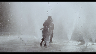
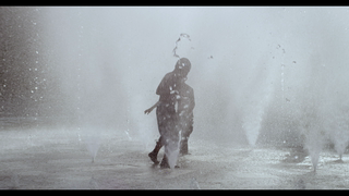
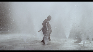
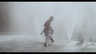
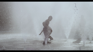
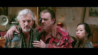
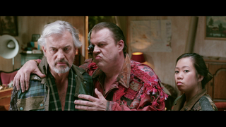
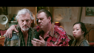
Figure 1: Consecutive frames of contents $\#11$ (top) and $\#203$ (bottom), respectively.

Furthermore, a viewer is said to be satisfied if one cannot perceive quality difference between the compressed clip and its anchor. The Satisfied User Ratio (SUR) of video clip $e_{i}$ on user group $j$ can be expressed as

$$Z_{i,j}=1-\frac{1}{|S_{j}|}\sum_{s\in S_{j}}\mathds{1}_{s}(e_{i}),$$ (3)

where $S_{j}$ is the $j-$th group of subjects and $|\cdot|$ denotes the cardinality. $\mathds{1}_{s}(e_{i})=1$ or $0$ if the $s-$th subject can or cannot see the difference between compressed clip $e_{i}$ and its anchor, respectively. The summation term in the right-hand-side of Eq. (3) is the empirical cumulative distribution function (CDF) of random variable $Y_{c,s}$. Then, by substituting Eq. (2) into Eq. (3), we obtain a compact expression for the SUR curve as

$$Z_{i,j}=Q(e_{i}|\mu_{Y},\sigma_{Y}^{2})=Q(e_{i}|y_{c}+b_{s},v_{c}^{2}+v_{s}^{2}),\quad\text{for}\quad s\in S_{j},$$ (4)

where $Q(\cdot)$ is the Q-function of the normal distribution. By dividing users into different groups, the model achieves small intra-group variance and large inter-group variance. We can model JND and SUR more precisely. Alternatively, a universal model could be generalized by replacing $S_{j}$ by the union of all subjects, i.e. $S=\bigcup_{j}S_{j}$.

4 Experimental results

We evaluate the performance of the proposed user model using real JND data from the VideoSet [8] and compare it with the MOS method. The VideoSet contains 220 video contents in four resolutions and three JND points per resolution per content. During the subjective test, the dataset was split into 15 subsets and each subset was evaluated independently by a group of subjects. The group size was around 35. We adopt a subset of the first JND point on 720p video in our experiment. It contains 15 video contents evaluated by 37 subjects.

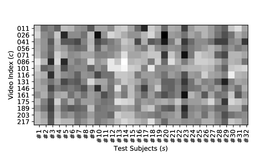
(a)

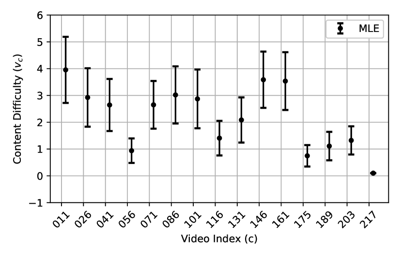
(b)

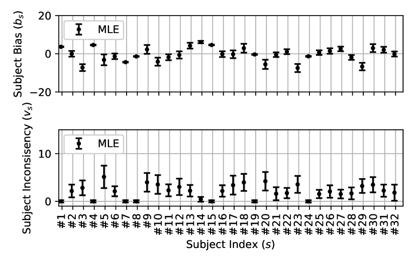
(c)

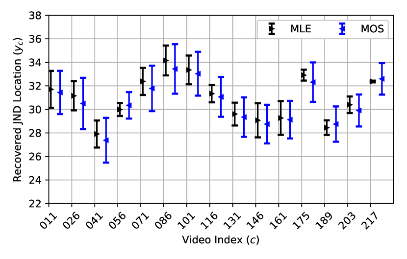
(d)

Figure 2: Visualization of cleaned JND data and estimated subject and content factors: (a) cleaned JND data, where each pixel represents one JND location and a brighter pixel means the JND happens at a larger QP, (b) estimated content difficulty (i.e. $v_{c}$) using the MLE method, (c) estimated subject bias and inconsistency (i.e. $v_{s}$), and (d) estimated JND locations using the MLE and the MOS methods, respectively. The error bars in subfigures represent $95\%$ confidence interval.

4.1 Parameter Inference

The cleaned JND scores are shown in Figure 2(a) and the estimated subject bias and inconsistency are shown in Figure 2(c), respectively. Please note that 5 subjects were identified as unreliable subjects and their quality votings were removed. These subjects have a larger bias value or inconsistent measures. We refer interested readers to [19] for further details.

Figure 2(b) shows the estimated content difficulty. Content $\#11$ is a scene about toddlers playing in a fountain. The masking effect is strong due to water drops in the background and moving objects. Thus, compression artifacts are difficult to perceive, and it has the highest content difficulty. On the other hand, content $\#203$ is a scene captured by a still camera. It focuses on speakers with blurred still background. The content difficulty is low as the masking effect is weak, and compression artifacts are more noticeable. Representative frame thumbnails are given in Fig. 1.

The estimated JND location using the MLE method and the MOS method are compared in Figure 2(d). The MLE approach offers more reliable estimation as its confidence intervals are much tighter than those estimated by the MOS method.

4.2 SUR on different viewer groups

We classify viewers into different viewer groups based on the estimated subject bias from cleaned JND data. The distribution of subject bias and inconsistency are given in Figure 3. The left and middle figures are the histogram of their statistics, respectively. For a large percentage of viewers, their bias and inconsistency are in a reasonable range (i.e. $[-4,4]$ for the subject bias and $[0,3.5]$ for subject inconsistency, respectively). The right figure is the scatter plot of these two factors. We do not observe strong correlation between them.

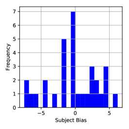
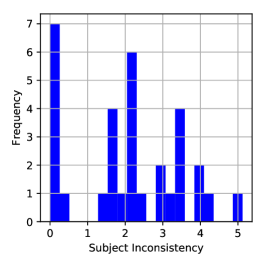
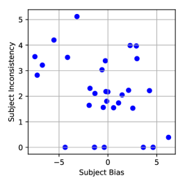
Figure 3: Illustration of subject factors. Left: the histogram of the subject bias. Middle: the histogram of subject inconsistency. Right: the scatter plot of subject inconsistency versus the subject bias.

In the following, we use video $\#11$ and $\#203$ as input contents to demonstrate the effectiveness of the proposed user model. Under fixed content factors, we compare the SUR differences between different viewer groups. Content $\#11$ has a strong masking effect so that it is difficult to evaluate (HC, “Hard Content”). Content $\#203$ has a weak masking effect and it is easy to evaluate (EC, “Easy Content”).

Figure 4 shows the effect of subject factors on the SUR curve. There are 6 SUR curves by combining different content factors and subject factors. The input parameters are obtained from MLE. They are set as follows.

• The subject bias is set to -4, 0, 4 for HS, NS and ES, respectively.

• Subject inconsistency is set to 2 for all subjects.

• The averaged JND locations are set to 31.7 and 30.39 for clip $\#11$ and $\#203$, respectively.

• The content difficulty levels are set to 3.962 and 1.326 for clip $\#11$ and $\#203$, respectively.

We have the following two observations.

1. SUR difference for normal users
   Consider the middle curves of EC and HC contents. Subjects in this group have normal sensitivity and we use this group to represent the majority. Intuitively, the content diversity is large if we visually examine those two clips. However, if we target at $SUR=0.75$, which is the counterpart of the mean value in the MOS method, the QP location from modeled SUR curve is pretty close. The difference increases when the SUR deviates from the $SUR=0.75$ location. For contents that have a weak masking effect (shown in blue curve), they are less resistant to compression distortion and SUR drops sharply once artifacts become noticeable. In contrast, for contents that have a strong masking effect (shown in red curve), they have better discriminatory power on subject capability so that the SUR curve drops slowly. Given the same extra bitrate quota, we could expect a higher SUR gain from EC than HC. It takes much more effort to satisfy critical users when the content has a strong masking effect. We conclude that it is essential to study content difficulty and subject capability to better model perceived quality of compressed video.

2. SUR difference for different user groups
   The SUR difference is considerably large among different user groups on the same content. We observe a gap between the three curves for both contents. The SUR curve of normal users is shifted by the subject bias $b_{s}$ in Eq. (4). Although the neutral user group covers the majority of users, we believe that a quality model would better characterize QoE by taking the user capability into consideration.

The above observations can be easily explained using the proposed user model. It shows the value and power of our study.

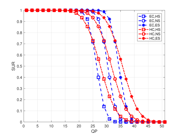
Figure 4: Illustration of the proposed user model. The blue and red curves demonstrate the SUR of EC and HC contents, respectively. For each content, the three curves show the SUR difference between different user groups.

5 Conclusion and future work

A flexible user model was proposed in this work by considering the subject and content factors in the JND framework. The QoE of a group of users was characterized by the Satisfied User Ratio (SUR) while the JND location of content $c$ from subject $s$ was modeled as a random variable parameterized by subject and content factors. The model parameters can be estimated by the MLE method using a set of JND-based subjective test data. As an application of the proposed user model, we studied SUR curves that are influenced by different user profiles and contents of different difficult levels. It was shown that the subject capability significantly affects the SUR curves, especially at the middle range of the quality curve.

Apparently, the proposed user model provides valuable insights on the quality assessment problem. We would like to explore these insights for better SUR prediction for new contents in the future.

References

- [1] ITU-R BT. 500, “Methodology for the subjective assessment of the quality of television pictures,” (2003).
- [2] ITU-T P.910, “Subjective video quality assessment methods for multimedia applications,” (1999).
- [3] Chen, K.-T., Wu, C.-C., Chang, Y.-C., and Lei, C.-L., “A crowdsourceable QoE evaluation framework for multimedia content,” in [Proceedings of the 17th ACM international conference on Multimedia ], 491–500, ACM (2009).
- [4] Ye, P. and Doermann, D., “Active sampling for subjective image quality assessment,” in [Proceedings of the IEEE Conference on Computer Vision and Pattern Recognition ], 4249–4256 (2014).
- [5] Whitehill, J., Wu, T.-f., Bergsma, J., Movellan, J. R., and Ruvolo, P. L., “Whose vote should count more: Optimal integration of labels from labelers of unknown expertise,” in [Advances in neural information processing systems ], 2035–2043 (2009).
- [6] Li, Q., Li, Y., Gao, J., Su, L., Zhao, B., Demirbas, M., Fan, W., and Han, J., “A confidence-aware approach for truth discovery on long-tail data,” Proceedings of the VLDB Endowment 8(4), 425–436 (2014).
- [7] Lin, J. Y., Jin, L., Hu, S., Katsavounidis, I., Li, Z., Aaron, A., and Kuo, C.-C. J., “Experimental design and analysis of JND test on coded image/video,” in [SPIE Optical Engineering+ Applications ], 95990Z–95990Z, International Society for Optics and Photonics (2015).
- [8] Wang, H., Katsavounidis, I., Zhou, J., Park, J., Lei, S., Zhou, X., Pun, M.-O., Jin, X., Wang, R., Wang, X., et al., “Videoset: A large-scale compressed video quality dataset based on JND measurement,” Journal of Visual Communication and Image Representation 46, 292–302 (2017).
- [9] Seshadrinathan, K., Soundararajan, R., Bovik, A. C., and Cormack, L. K., “Study of subjective and objective quality assessment of video,” IEEE Transactions on Image Processing 19(6), 1427–1441 (2010).
- [10] Group, V. Q. E. et al., “Report on the validation of video quality models for high definition video content,” VQEG, Geneva, Switzerland, Tech. Rep.[Online]. Available: http://www. its. bldrdoc. gov/vqeg/projects/hdtv/hdtv. aspx (2010).
- [11] Lin, J. Y., Song, R., Wu, C.-H., Liu, T., Wang, H., and Kuo, C.-C. J., “MCL-V: A streaming video quality assessment database,” Journal of Visual Communication and Image Representation 30, 1 – 9 (2015).
- [12] Li, Z. and Bampis, C. G., “Recover subjective quality scores from noisy measurements,” in [Data Compression Conference (DCC), 2017 ], 52–61, IEEE (2017).
- [13] Janowski, L. and Pinson, M., “The accuracy of subjects in a quality experiment: A theoretical subject model,” IEEE Transactions on Multimedia 17(12), 2210–2224 (2015).
- [14] Wu, Q., Li, H., Meng, F., and Ngan, K. N., “A perceptually weighted rank correlation indicator for objective image quality assessment,” IEEE Transactions on Image Processing 27, 2499–2513 (May 2018).
- [15] Jin, L., Lin, J. Y., Hu, S., Wang, H., Wang, P., Katasvounidis, I., Aaron, A., and Kuo, C.-C. J., “Statistical study on perceived JPEG image quality via MCL-JCI dataset construction and analysis,” in [IS&T/SPIE Electronic Imaging ], International Society for Optics and Photonics (2016).
- [16] Wang, H., Gan, W., Hu, S., Lin, J. Y., Jin, L., Song, L., Wang, P., Katsavounidis, I., Aaron, A., and Kuo, C.-C. J., “MCL-JCV: A JND-based H.264/AVC video quality assessment dataset,” in [2016 IEEE International Conference on Image Processing (ICIP) ], 1509–1513 (Sept 2016).
- [17] Huang, Q., Wang, H., Lim, S. C., Kim, H. Y., Jeong, S. Y., and Kuo, C.-C. J., “Measure and prediction of hevc perceptually lossy/lossless boundary QP values,” in [Data Compression Conference (DCC), 2017 ], 42–51, IEEE (2017).
- [18] Wang, H., Katsavounidis, I., Huang, Q., Zhou, X., and Kuo, C.-C. J., “Prediction of satisfied user ratio for compressed video,” arXiv preprint arXiv:1710.11090 (2017).
- [19] Wang, H., Zhang, X., Yang, C., and Kuo, C.-C. J., “A JND-based video quality assessment model and its application,” arXiv preprint arXiv:1807.00920 (2018).