Modulation-Domain Kalman Filtering for Monaural Blind Speech Denoising and Dereverberation

Abstract

We describe a monaural speech enhancement algorithm based on modulation-domain Kalman filtering to blindly track the time-frequency log-magnitude spectra of speech and reverberation. We propose an adaptive algorithm that performs blind joint denoising and dereverberation, while accounting for the inter-frame speech dynamics, by estimating the posterior distribution of the speech log-magnitude spectrum given the log-magnitude spectrum of the noisy reverberant speech. The Kalman filter update step models the non-linear relations between the speech, noise and reverberation log-spectra. The Kalman filtering algorithm uses a signal model that takes into account the reverberation parameters of the reverberation time, $T_{60}$, and the direct-to-reverberant energy ratio (DRR) and also estimates and tracks the $T_{60}$ and the DRR in every frequency bin in order to improve the estimation of the speech log-magnitude spectrum. The Kalman filtering algorithm is tested and graphs that depict the estimated reverberation features over time are examined. The proposed algorithm is evaluated in terms of speech quality, speech intelligibility and dereverberation performance for a range of reverberation parameters and SNRs, in different noise types, and is also compared to competing denoising and dereverberation techniques. Experimental results using noisy reverberant speech demonstrate the effectiveness of the enhancement algorithm.

N. Dionelis and M. Brookes are with the Department of Electrical and Electronic Engineering, Imperial College London, London SW7 2AZ, U.K. (e-mail: nikolaos.dionelis11@imperial.ac.uk; mike.brookes@imperial.ac.uk).

I Introduction

Nowadays, technology is ever evolving with tremendous haste and the demand for speech enhancement systems is evident. Speech enhancement in noisy reverberant environments, for human listeners, is challenging. Speech is degraded by noise and reverberation when captured using a near-field or far-field distant microphone [1] [2]. A room impulse response (RIR) can include components at long delays, hence resulting in reverberation and echoes [3] [4]. Reverberation is a convolutive distortion that can be quite long with a reverberation time, $T_{60}$, of more than $0.8$ s. Due to convolution, reverberation induces long-term correlation between consecutive observations. Reverberation and noise, which can be stationary or non-stationary, have a detrimental impact on speech quality and intelligibility. Reverberation, especially in the presence of non-stationary noise, damages the intelligibility of speech.

The direct to reverberant energy ratio (DRR) and the reverberation time, $T_{60}$, are the two main parameters of a reverberation model [5] [1]. The DRR describes reverberation in the space domain, depending on the positions of the sound source and the receiver. The $T_{60}$ is the time interval required for a sound level to decay $60$ dB after ceasing its original stimulus. The reverberation time, when measured in the diffuse sound field, is independent of the source to microphone configuration and mainly depends on the room. The impact of reverberation on auditory perception depends on the $T_{60}$. If the $T_{60}$ is short, the environment reinforces the sound which may enhance the sound perception [6] [7]. On the contrary, if the $T_{60}$ is long, spoken syllables interfere with future spoken syllables. Reverberation spreads energy over time and this smearing across time has two effects: (a) the energy of individual phonemes spreads out in time and, hence, plosives have a delayed decay and fricatives are smoothed, and (b) preceding phonemes blur into the current phonemes.

The aim of speech enhancement is to reduce and ideally eliminate the effects of both noise and reverberation without distorting the speech signal [8]. Enhancement algorithms typically aim to suppress noise and late reverberation because early reverberation is not perceived as separate sound sources and usually improves the quality and intelligibility of speech. Noise is assumed to be uncorrelated with speech, early reverberation is correlated with speech and late reverberation is commonly assumed to be uncorrelated with speech [9] [6].

Speech enhancement can be performed in different domains. The ideal domain should be chosen such that (a) good statistical models of speech and noise exist in this domain, and (b) speech and noise are separable in this domain. Speech and noise are additive in the time domain and the Short Time Fourier Transform (STFT) domain [10] [11]. The relation between speech and noise becomes progressively more complicated in the amplitude, power and log-power spectral domains. Noise suppression algorithms usually operate in a time-frequency STFT domain and these techniques have been extended to address dereverberation. In [9], spectral enhancement methods based on a time-frequency gain, originally developed for noise suppression, have been modified and employed for dereverberation. Such algorithms suppress late reverberation assuming that the early and late reverberation components are uncorrelated. The spectral enhancement methods in [12] [9] estimate the late reverberant spectral variance (LRSV) and use it in the place of the noise spectral variance, reducing the problem of late reverberation suppression to that of estimating the LRSV [6]. In [7], blind spectral weighting is employed to reduce the overlap-masking effect of reverberation using an uncorrelated and additive assumption for late reverberation.

Dereverberation algorithms that leave the phase unaltered and operate in the amplitude, power or log-power spectral domains are relatively insensitive to minor variations in the spatial placement of sources [13]. Two criticisms of spectral enhancement algorithms based on LRSV reverberation noise estimation are that they introduce musical noise and suppress speech onsets when they over-estimate reverberation [14]. The LRSV estimator in [15], which is a continuation of [6], models the RIR in the STFT domain and not in the time domain [6] [16], using the same model of the RIR that is attributed to J. Polack or J. Moorer [16]. Reverberation is estimated in [15] considering the STFT energy contribution of the direct path of speech and an external $T_{60}$ estimate.

Modelling the speech temporal dynamics is beneficial when the $T_{60}$ is long and the DRR is low [17] [2]. Joint denoising and dereverberation using speech and noise tracking is performed in [17]. The SPENDRED algorithm [18] [19], which is a model-based method with a convolution model for reverberation based on the $T_{60}$ and the DRR, considers the speech temporal dynamics. SPENDRED employs a parametric model of the RIR [20] and performs frequency-dependent and time-varying $T_{60}$ and DRR estimation. However, unless the source or the microphone are moving, the $T_{60}$ and the DRR will be constant throughout the recording. The SPENDRED algorithm assumes that $\text{DRR}\geq 1-(10^{-6})^{\frac{L}{T_{60}}}$ where $L$ is the acoustic frame increment. For example, when $T_{60}=0.4$ s and $L=5$ ms, then $\text{DRR}\geq-8$ dB is assumed. In addition, SPENDRED performs intra-frame correlation modelling, which can be beneficial in adverse conditions, while typical algorithms decouple different frequency dimensions [10].

Statistical-based models, such as the SPENDRED algorithm, describe reverberation by a convolution in the power spectral domain while LRSV models describe reverberation as an additive distortion in the power spectral domain [20] [21]. A model with an infinite impulse response is used either with the two parameters of the $T_{60}$ and the DRR, as in [18] [19], or with a finite number of parameters. The infinite-order convolution model of reverberation with the $T_{60}$ and the DRR is sparse and contrasts with the higher-order autoregressive processes in the complex STFT domain, used in [22] [23].

The algorithms described in [24], [20] and [21] create non-linear observation models of noisy reverberant speech in the log Mel-power spectral domain, using the reverberation-to-noise ratio (RNR). As discussed in [25], phase differences in Mel-frequency bands have different properties from phase differences in STFT bins. The phase factor between reverberant speech and noise is different from that between speech and noise [24]. In [20], the phase factor between reverberant speech and noise in Mel-frequency bands is examined.

In noisy reverberant conditions, finding the onset of speech phonemes and determining which frames are unvoiced/silence is difficult, due to the smearing across time, often leading to noise over-estimation. The concatenation of different techniques for denoising and dereverberation has lower performance than unified methods due to over-estimating noise when estimating noise and reverberation separately [17] [26].

Despite the claim that it is inefficient to perform a two step procedure that is comprised of denoising followed by dereverberation [17] [26], long-term linear prediction with pre-denoising can be used to suppress noise and reverberation. With the weighted prediction error (WPE) algorithm [27] [2], reverberation is represented as a one-dimensional convolution in each frequency bin. In [28], the WPE algorithm is discussed along with inter-frame correlation. In [29], the WPE algorithm is used in the complex STFT domain performing batch processing and iteratively estimating, first, the reverberation prediction coefficients and, then, the speech spectral variance. The WPE linear filtering approach, which can be employed in the power spectral domain [30] [31], takes into account past frames, from the $3$-rd to the $40$-th past frame [29] [30].

This paper presents an adaptive denoising and dereverberation Kalman filtering framework that tracks the speech and reverberation spectral log-magnitudes. In this paper, we extend the enhancer in [32] to include dereverberation. Enhancement is performed using a Kalman filter (KF) to model inter-frame correlations. We use an integrated structure of two parallel signal models to track speech, reverberation and the $T_{60}$ and DRR reverberation parameters. The $T_{60}$ and the DRR are updated in every frame to improve the estimation of the speech log-magnitude spectrum. We create an observation model and a series of non-linear KF update steps performing joint noise and reverberation suppression by estimating the first two moments of the posterior distribution of the speech log-spectrum given the noisy reverberant log-spectrum. The log-spectral domain is chosen, as in [33] [32], because good speech models exist in this domain. Modelling spectral log-amplitudes as Gaussian distributions leads to good speech modelling in noisy reverberant environments since super-Gaussian distributions that resemble the log-normal, such as the Gamma [11] [34], are used to model the speech amplitude spectrum. Mean squared errors (MSEs) in the log-spectral domain are a good measure to use for perceptual quality and speech log-spectra are well modelled by Gaussian distributions, as in [35] and [36].

The structure of this paper is as follows. Section II describes the signal model and Sec. III presents the enhancement algorithm and its non-linear KF. The implementation and the validation of the algorithm are in Sec. IV. The algorithm’s evaluation is in Sec. V. Conclusions are drawn in Sec. VI.

II Signal model and notation

In the complex STFT domain, the noisy speech, $Y_{t}(k)$, is given by $Y_{t}(k)=S_{t}(k)+R_{t}(k)+N_{t}(k)$ where $S_{t}(k)$ is the direct speech component, $R_{t}(k)$ is the reverberant speech component and $N_{t}(k)$ is the noise, as for example in [22] [23]. The time-frame index is $t$ and the frequency bin index is $k$. For clarity, we also define $Z_{t}(k)=R_{t}(k)+N_{t}(k)$. We drop the time and frequency indexes and we obtain $Y=S+Z=S+R+N$. We define the log-magnitude spectrum of $S$ as $s=\log(|S|)$ and we also define $r$, $n$, $y$ and $z$ similarly.

In the signal model, signal quantities with capital letters, such as $S_{t}$, are complex numbers with magnitude and phase values, $|S_{t}|$ and $\angle S_{t}$. In the complex STFT domain, using $a_{t},b_{t}\in\mathbb{R}$, the reverberation signal model is given by

$$R_{t} =\sqrt{a_{t}}\,R_{t-1}\exp(j\theta_{t})+\sqrt{b_{t}}\,S_{t-1}\exp(j\psi_{t})$$ (1)

$$=\sum_{\tau=1}^{\infty}\left(\prod_{i=1}^{\tau-1}\left(\sqrt{a_{t-i+1}}\exp(j\theta_{t-i+1})\right)\right.$$

$$\times\left.\sqrt{b_{t-\tau+1}}S_{t-\tau}\exp(j\psi_{t-\tau+1})\right)\text{,}$$

$$a_{t}^{\frac{T_{60}}{L}}=10^{-6},\ \ \ \ \ \ \ \ b_{t}=\frac{1-a_{t}}{\text{DRR}}$$ (2)

where $L$ is the acoustic frame increment. In (1), the factors $\exp(j\theta_{t})$ and $\exp(j\psi_{t})$, where $\theta_{t}$ and $\psi_{t}$ are uniformly distributed phases, are used. In (2), the DRR is defined in the power spectral domain [18] [19] and the $T_{60}$ and the DRR are both time and frequency dependent, as described in [5].

The expression in (1) is the convolution model for reverberation; the most common reverberation model is this single-pole filter that is described by the pole and zero positions that depend on the $T_{60}$ and the DRR [18] [2]. A convolution of infinite order is used, with the two parameters of the $T_{60}$ and the DRR, to describe reverberation [18] [19]. Models that describe reverberation by a convolution are also discussed in [20] [21]. The signal model is defined by (1) and by

$$Y_{t}=S_{t}+Z_{t},\ \ \ \ \ \ Z_{t}=R_{t}+N_{t}\text{,}$$ (3)

$$\gamma_{t}=0.5\log\left(a_{t}\right),\ \ \delta_{t}=\gamma_{t}+r_{t-1}=\log\left(\sqrt{a_{t}}\left|R_{t-1}\right|\right)\text{,}$$ (4)

$$\beta_{t}=0.5\log\left(b_{t}\right),\ \ \epsilon_{t}=\beta_{t}+s_{t-1}=\log(\sqrt{b_{t}}\left|S_{t-1}\right|)$$ (5)

where $b_{t}>0$, $0<a_{t}<1$ and $\gamma_{t}<0$.

Figure 1 shows graphs of $\beta$ against $T_{60}$ for a fixed DRR and of $\beta$ against DRR for a fixed $T_{60}$. If $\text{DRR}=0$ dB, then $b_{t}=1-a_{t}$. If $\beta_{t}=0$, then $b_{t}=1$ and $\text{DRR}=1-a_{t}$.

Figure 2 illustrates the flowchart of the signal model. The reverberation signal model in (1) uses $\sqrt{a_{t}}$ and $\sqrt{b_{t}}$ because the $a_{t}$ and $b_{t}$ reverberation parameters, in (2), and the DRR are defined in the power spectral domain, as in [18] [19]. The $a_{t}$ and $b_{t}$ parameters are mapped to $\gamma_{t}$ and $\beta_{t}$ using (4) and (5). The signals $z_{t}$, $\delta_{t}$ and $\epsilon_{t}$ are the total distubance, the old (decaying) reverberation and the new reverberation, respectively. We note that $z_{t}$ is defined in the first paragraph of this section and that $\delta_{t}$ and $\epsilon_{t}$ are defined in (4) and (5).

The signal model of how the reverberation parameters of $\gamma_{t}$ and $\beta_{t}$ change over time is a random walk model. This is used in the algorithm’s KF prediction step for $\gamma_{t}$ and $\beta_{t}$.

The signal model in Fig. 2 is directly linked to the alternating and interacting KFs of the enhancement algorithm. The algorithm is a collection of two KFs, the speech KF and the reverberation KF, that estimate the speech and reverberation log-amplitude spectra and the $\gamma_{t}$ and $\beta_{t}$ reverberation parameters. This KF algorithm is described in detail in Sec. III.

III The speech enhancement algorithm

The KF algorithm operates in the log-magnitude spectral domain, tracking speech and reverberation. Figure 3 depicts the denoising and dereverberation algorithm that formulates a model of reverberation as a first-order autoregressive process and propagates the means and variances of the random variables. Almost all the signals follow a Gaussian distribution and the distribution of $s_{t}$ conditioned on observations up to time $\tau$ is given by $p_{s_{t|\tau}}(s)\triangleq p(s_{t}|y_{0},\dots,y_{\tau})=N(s_{t|\tau},\Sigma^{(s)}_{t|\tau})$. In Fig. 3, a Gaussian distribution is denoted by its mean, $s_{t|\tau}$.

The core of the algorithm in Fig. 3 is the KF that is defined by the gray blocks in the flowchart diagram. The non-linear KF estimates and tracks the posterior distributions of the speech log-magnitude spectrum, $s_{t}$, the reverberation log-magnitude spectrum, $r_{t}$, and the reverberation parameters, $\gamma_{t}$ and $\beta_{t}$.

The input to the algorithm in Fig. 3 is the noisy reverberant speech in the time domain. The algorithm’s first step is to perform a STFT and obtain the signal in the complex STFT domain. The algorithm does not alter the noisy reverberant phase, $\angle Y$, and uses the noisy reverberant amplitude spectrum, $|Y|$, in three ways: in the speech KF prediction step, in the KF update step and in the noise power modelling. The main part of the algorithm is the KF and the speech KF state, $\textbf{s}_{t}\in\mathbb{R}^{p}$, is the speech log-spectrum from the previous $p$ frames,

$$\textbf{s}_{t}=(s_{t}\ s_{t-1}\ \dots\ s_{t-p+1})^{T}\text{.}$$ (6)

The speech KF prediction step is based on autoregressive (AR) modelling on the log-spectrum of pre-cleaned speech [33]. The reverberation KF state is $r_{t}$ and the KF states of the reverberation parameters are $\gamma_{t}$ and $\beta_{t}$. The KF observation is the noisy reverberant speech log-spectrum, $y_{t}$, which is used in the KF update step to compute the first two moments of the posterior of the speech log-spectrum. The mean of the speech log-spectrum posterior is used together with $\angle Y$ to create the enhanced speech signal using the inverse STFT (ISTFT).

Apart from the speech log-spectrum, the non-linear KF also tracks the reverberation log-spectrum, $r_{t}$, and the $\gamma_{t}$ and $\beta_{t}$ reverberation parameters. The KF, as defined by the gray blocks in Fig. 3, has a speech KF prediction step, a reverberation KF prediction step and a series of KF update steps. The reverberation KF is comprised of the blocks “Reverberation KF prediction”, “KF Update” and “$\gamma_{t}$, $\beta_{t}$ KF Update”. These three blocks perform joint denoising and dereverberation and estimate $s_{t|t}$ and $\Sigma_{t|t}^{\text{(s)}}$ to enhance noisy reverberant speech.

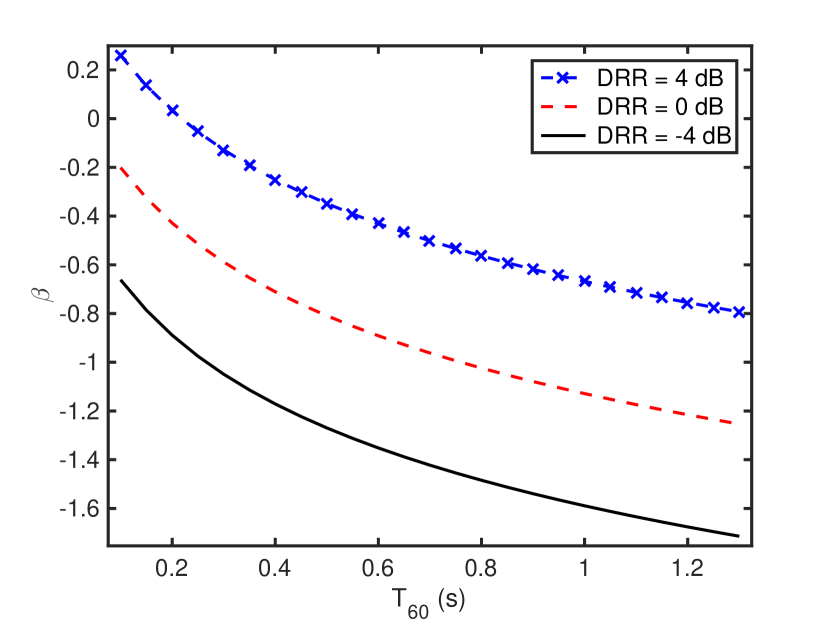
(a)

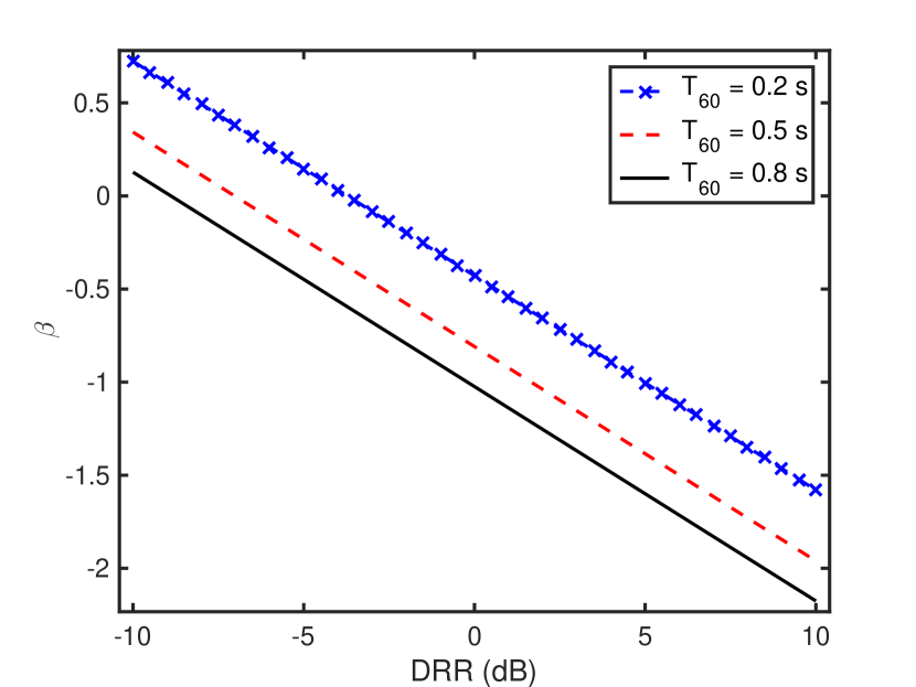
(b)

Figure 1: Plot of $\beta$, using $L=8$ ms in (2), against: (a) $T_{60}$ when the DRR is $4$, $0$ and $-4$ dB, and (b) DRR when the $T_{60}$ is $0.2$, $0.5$ and $0.8$ s.

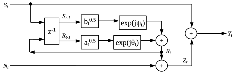
Figure 2: The flowchart diagram of the proposed signal model of the speech enhancement algorithm. The signal model is defined in (1) and (3).

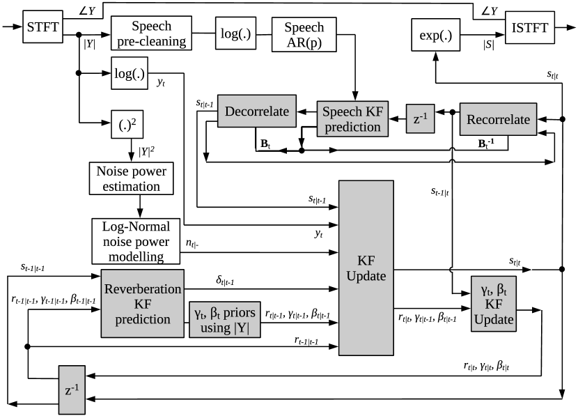
Figure 3: The flowchart of the algorithm to suppress noise and reverberation. For clarity, the signal variances are not included. The gray blocks constitute the KF that tracks the speech and reverberation log-spectra and the reverberation parameters. The “KF Update” and “$\gamma_{t}$, $\beta_{t}$ KF Update” blocks constitute the non-linear KF update step that uses the signal model described in Sec. II.

The structure of the rest of this algorithm description section is as follows. Sections III.A and III.B present the speech and reverberation KF prediction steps, respectively. Section III.C describes the KF update step and Sec. III.D the priors for the $\gamma_{t}$ and $\beta_{t}$ parameters that are needed so that the KF (a) distinguishes between speech and reverberation, and (b) does not diverge to non-realistic $T_{60}$ and DRR estimates. Section III.E describes the unshaded peripheral blocks in Fig. 3.

III-A The Speech KF Prediction Step

The speech KF prediction step is linear and is related to the “Speech KF prediction”, “Decorrelate” and “Recorrelate” blocks in Fig. 3. The speech KF prediction step is described in [33] and in [32] [35] and is based on conditional distributions to model short-term dependencies. Decorrelation and recorrelation of the speech KF state in (6) are performed after and before the speech KF prediction step, respectively. The decorrelation and recorrelation operations in Fig. 3, which are performed so that the non-linear KF update step can be applied, perform vector-matrix and matrix-matrix multiplications for the speech KF state mean and its covariance matrix, respectively, using $\textbf{B}_{t}\in\mathbb{R}^{p\times p}$ [34] [33]. The outputs of the “Decorrelate” block are: (a) the first element of the speech KF state, and (b) the rest elements of the speech KF state.

The KF prediction step propagates the first and second moments of the speech KF state [33] [36]. Inter-frame linear relationships are used for the speech KF prediction step that uses AR modelling in the log-magnitude spectral domain. In the speech KF prediction step, $\textbf{s}_{t}$ is predicted as a linear combination of $\textbf{s}_{t-1}$ using the speech AR coefficients that are obtained from the “Speech AR(p)” block in Fig. 3, which uses pre-cleaned speech as an input. After the speech KF prediction step, $\textbf{s}_{t}$ is correlated; we decorrelate the speech KF state with a linear transformation (using $\textbf{B}_{t}$) to simplify the KF update step and impose the observation constraint [10]. The KF update step changes only the first element of the speech KF state and after the KF update step, recorrelation is applied with a linear transformation (using $\textbf{B}_{t}^{-1}$) to continue the KF recursion.

III-B The Reverberation KF Prediction Step

The presented algorithm uses a KF prediction step for $\gamma_{t}$ and $\beta_{t}$ that assumes that the variance of $\gamma_{t}$ and $\beta_{t}$ increases over time, preserving their mean. The KF algorithm implements a random-walk prediction step, performing the operations of

$$\negthinspace\negthinspace\negthinspace\negthinspace\negthinspace\negthinspace\negthinspace\negthinspace\negthinspace\negthinspace\gamma_{t|t-1}^{\prime}=\gamma_{t-1|t-1},\ \ \ \ \ \Sigma_{t|t-1}^{(\gamma^{\prime})}=\Sigma_{t-1|t-1}^{(\gamma)}+Q_{\gamma},$$ (7)

$$\negthinspace\negthinspace\negthinspace\negthinspace\negthinspace\negthinspace\negthinspace\negthinspace\negthinspace\negthinspace\beta_{t|t-1}^{\prime}=\beta_{t-1|t-1},\ \ \ \ \ \Sigma_{t|t-1}^{(\beta^{\prime})}=\Sigma_{t-1|t-1}^{(\beta)}+Q_{\beta}$$ (8)

where $Q_{\gamma}$ is a fixed error variance for $\gamma$ and $Q_{\beta}$ is a fixed error variance for $\beta$. The values used for the prediction error variances, $Q_{\gamma}$ and $Q_{\beta}$, depend on the rate at which the $T_{60}$ and the DRR are likely to change in a real situation.

After the reverberation KF prediction step, the algorithm computes and imposes priors on $\gamma_{t}$ and $\beta_{t}$ using Gaussian-Gaussian multiplication. The internally computed priors for $\gamma_{t}$ and $\beta_{t}$ in the “$\gamma_{t}$, $\beta_{t}$ priors” block in Fig. 3 are explained in Sec. III.D. After imposing the priors, the outputs are $\gamma_{t|t-1}$, $\Sigma_{t|t-1}^{(\gamma)}$ and $\beta_{t|t-1}$, $\Sigma_{t|t-1}^{(\beta)}$. We note that a prime diacritic, $\prime$, is used in (7) and (8) to denote quantities before the priors.

The “Reverberation KF prediction” block in Fig. 3 estimates the first two moments of the prior distribution of the reverberation spectral log-amplitude, i.e. $r_{t|t-1}$ and its variance. The algorithm performs a reverberation KF prediction step based on the previous posterior of both speech and reverberation using the signal model in (1), where $a$ is less than unity and this makes the reverberation KF prediction step stable.

From (1) and Fig. 2, the STFT-domain reverberation is the sum of two components arising, respectively, from the reverberation and speech components of the previous frame. The old reverberation, $\delta_{t}$, and the new reverberation, $\epsilon_{t}$, are defined in (4) and (5), respectively. The KF algorithm calculates the prior distributions of these two components in the log-amplitude spectral domain using $\delta_{t|t-1}=\gamma_{t|t-1}+r_{t-1|t-1}$ and $\epsilon_{t|t-1}=\beta_{t|t-1}+s_{t-1|t-1}$. These equations are based on (4) and (5) with a common condition added to all terms. Assuming that $r_{t-1}$ and $s_{t-1}$ are uncorrelated with $\gamma_{t}$ and $\beta_{t}$, respectively, the means and variances of the two Gaussian distributions are added. The variances therefore add,

$$\Sigma_{t|t-1}^{(\delta)}=\Sigma_{t|t-1}^{(\gamma)}+\Sigma_{t-1|t-1}^{\text{(r)}},$$ (9)

$$\Sigma_{t|t-1}^{(\epsilon)}=\Sigma_{t|t-1}^{(\beta)}+\Sigma_{t-1|t-1}^{\text{(s)}}\text{.}$$ (10)

As shown in Fig. 3, the final operation of the “Reverberation KF prediction” block is to compute the prior distribution, $r_{t|t-1}$. The addition in the complex STFT domain of two random variables in the log-spectral domain is modelled. The reverberation log-amplitude spectrum is estimated by modelling the addition in the STFT domain of two random variables in the log-amplitude spectral domain. Given two disturbance sources, we combine them into a single disturbance source.

From this point onwards in Sec. III.B, the time-frame subscript $t|t-1$ is omitted for clarity. For example, $p(\delta)$ is used instead of $p_{\delta_{t|t-1}}(\delta)$, which is defined in Sec. III.

From (1), the reverberation component is the STFT-domain sum of two elements arising, respectively, from the reverberation and speech components in the previous frame. The log-amplitude spectral domain distributions of these two elements, $\delta_{t|t-1}$ and $\epsilon_{t|t-1}$, were calculated in the preceding paragraphs. A two-dimensional Gaussian distribution is used for $p(\delta,\epsilon)=p(\delta)p(\epsilon)$ assuming independence between $\delta$ and $\epsilon$. We assume that the phase difference, $\eta$, between the two disturbance sources, $\delta$ and $\epsilon$, is uniformly distributed, i.e. $\eta\sim U(-\pi,\pi)$, and independent of their magnitudes. We write $e^{2r}=e^{2\delta}+e^{2\epsilon}+2\cos(\eta)e^{\delta+\epsilon}$ and $r=0.5\log\left(e^{2\delta}+e^{2\epsilon}+2\cos(\eta)e^{\delta+\epsilon}\right)$, which takes account of $\eta$ [32] [33]. Next, we calculate

$$\mathbb{E}\left\{r\right\} =\int_{\eta=-\pi}^{\pi}p(\eta)\ \int_{\delta,\epsilon}r\ p(\delta,\epsilon)\ d\delta\ d\epsilon\ d\eta$$

$$=\int_{\eta=0}^{\pi}\dfrac{1}{\pi}\ \int_{\delta,\epsilon}0.5\log\left(e^{2\delta}+e^{2\epsilon}+2\cos(\eta)e^{\delta+\epsilon}\right)$$

$$\times p(\delta)\ p(\epsilon)\ d\delta\ d\epsilon\ d\eta\text{,}$$ (11)

$$\mathbb{E}\left\{r^{2}\right\} =\int_{\eta=0}^{\pi}\dfrac{1}{\pi}\ \int_{\delta,\epsilon}\left(0.5\log\left(e^{2\delta}+e^{2\epsilon}\right.\right.$$

$$\left.\left.+2\cos(\eta)e^{\delta+\epsilon}\right)\right)^{2}\times p(\delta)\ p(\epsilon)\ d\delta\ d\epsilon\ d\eta$$ (12)

where $K_{(\delta,\epsilon)}$ sigma points are used to evaluate the inner integral over $(\delta,\epsilon)$ [37] and $K_{\eta}$ the outer integral over $\eta$.

Equations (11) and (12) estimate the first two moments of the prior distribution of reverberation, $r_{t|t-1}$. In this algorithm description section, we provide expressions for either the second moment or the variance. We convert implicitly between them using, for example, $\Sigma_{t}^{\text{(r)}}=\mathbb{E}\{r_{t}^{2}\}-(\mathbb{E}\{r_{t}\})^{2}$ for $r_{t}$.

III-C The Non-Linear KF Update Step

The KF algorithm decomposes the noisy reverberant observation, $y_{t}$, into its component parts using distributions in the log-magnitude spectral domain. The decompositions are based on Fig. 2 and the signal model in (3) and (1). The KF algorithm performs a series of low-dimensional operations instead of a high-dimensional one in the KF update step. The adaptive KF algorithm propagates backwards through Fig. 2 and decomposes: (a) $y_{t}$ into speech, $s_{t}$, and into reverberation and noise, $z_{t}$, (b) the reverberation and noise, $z_{t}$, into reverberation, $r_{t}$, and into noise, $n_{t}$, and (c) the reverberation, $r_{t}$, into “old reverberation”, $\delta_{t}$, and into “new reverberation”, $\epsilon_{t}$. The reverberation and noise log-spectrum, $z_{t}$, is a variable of the “KF Update” block in Fig. 3.

The KF algorithm in Fig. 3 uses the noisy reverberant observation, $y_{t}$, to first update $s_{t}$ and $z_{t}$ and then update $r_{t}$. The posterior $z_{t|t}$ is computed in the “KF Update” block in Fig. 3. In the proposed KF algorithm, the observed $y_{t}$ affects $z_{t|t}$ directly and, in turn, $z_{t|t}$ affects $r_{t|t}$. We hence divide the observation update into two steps: (a) we use the log-spectrum observation, $y_{t}$, to estimate the posterior distributions $s_{t|t}$ and $z_{t|t}$ because $Y_{t}=S_{t}+Z_{t}$ in (3), and (b) we use $z_{t|t}$ as an “observation” to obtain the posterior distributions $r_{t|t}$ and $n_{t|t}$ because $Z_{t}=R_{t}+N_{t}$ in (3). In (b), we calculate an updated version of $r_{t}$ by using the posterior $z_{t|t}$ as a KF observation constraint. Hence, according to (a) and (b), the log-spectrum observation, $y_{t}$, provides new information about $s_{t}$ and $r_{t}$.

The sequence of operations involved in the “Reverberation KF prediction”, “KF update” and “$\gamma_{t}$, $\beta_{t}$ KF update” blocks are listed in Table LABEL:tab:ppssaaa. The “Reverberation KF prediction” block in Fig. 3, which was presented in Sec. III.B, performs the first five operations in Table LABEL:tab:ppssaaa. The “KF update” and “$\gamma_{t}$, $\beta_{t}$ KF update” blocks in Fig. 3 perform the next seven operations in Table LABEL:tab:ppssaaa, i.e. steps 6-12. The bottom “$z^{-1}$” block in Fig. 3 performs step 13. These 13 steps constitute the dereverberation KF update step. The non-linear dereverberation KF update step computes the first two moments of the posterior distributions for most signal quantities and, moreover, includes the prediction step as well for some quantities. Both means and variances are computed for the tracked Gaussian signals; for clarity, the variances, such as $\Sigma_{t|t}^{\text{(r)}}$ for $r_{t}$, are not included in Table LABEL:tab:ppssaaa.

[caption = The operations performed in the “Reverberation KF prediction”, “KF Update” and “$\gamma_{t}$, $\beta_{t}$ KF Update” blocks in Fig. 3. Steps 7-12 perform specific signal decompositions propagating backwards through Fig. 2., label = tab:ppssaaa, pos = hp, doinside=, width=.492]p0.2cm p7.8cm & Inputs: (a) $s_{t|t-1}$ from the speech KF prediction step, (b) $n_{t|-}$ from external noise estimation, (c) $y_{t}$ from observation, and (d) $s_{t-1|t}$ from $s_{t|t}$ in step 7 and $\textbf{B}_{t}^{-1}$ from Sec. III.A. 1: $\gamma_{t|t-1}\ \leftarrow\ \gamma_{t-1|t-1}$ from step 13 2: $\beta_{t|t-1}\ \leftarrow\ \beta_{t-1|t-1}$ from step 13 3: $\delta_{t|t-1}\ \leftarrow\ \gamma_{t|t-1},r_{t-1|t-1}$ from steps 1, 13 4: $\epsilon_{t|t-1}\ \leftarrow\ \beta_{t|t-1},s_{t-1|t-1}$ from steps 2, 13 5: $r_{t|t-1}\ \leftarrow\ \delta_{t|t-1},\epsilon_{t|t-1}$ from steps 3, 4 6: $z_{t|t-1}\ \leftarrow\ r_{t|t-1},n_{t|-}$ from step 5 and input (b) 7: $s_{t|t},z_{t|t}\ \leftarrow\ s_{t|t-1},z_{t|t-1},y_{t}$ from 6 and inputs (a), (c) 8: $r_{t|t},[n_{t|t}]\ \leftarrow\ r_{t|t-1},n_{t|-},z_{t|t}$ from 5, 7 and input (b) 9: $\epsilon_{t|t}^{\prime}\ \leftarrow\ \beta_{t|t-1},s_{t-1|t}$ from step 2 and input (d) 10: $\delta_{t|t},\epsilon_{t|t}\ \leftarrow\ \delta_{t|t-1},\epsilon_{t|t}^{\prime},r_{t|t}$ from steps 3, 8, 9 11: $\gamma_{t|t},[r_{t-1|t}]\ \leftarrow\ \gamma_{t|t-1},r_{t-1|t-1},\delta_{t|t}$ from steps 1, 10, 13 12: $\beta_{t|t},[s_{t-1|t}]\ \leftarrow\ \beta_{t|t-1},s_{t-1|t},\epsilon_{t|t}$ from 2, 10 and input (d)13: $r_{t-1|t-1},\gamma_{t-1|t-1},\beta_{t-1|t-1}\ \leftarrow\ r_{t|t},\gamma_{t|t},\beta_{t|t}$

For clarity, from this point onwards in Sec. III.C, the time subscript is included only if it differs from $t|t-1$. Table LABEL:tab:ppssaaa shows the time subscripts. We also denote $n_{t|-}$ by $n_{t|t-1}$.

The KF algorithm computes the total distubance, $z_{t}$, from (3) in step 6 using similar equations to step 5. A two-dimensional Gaussian distribution is used for $p(r,n)$ and independence is assumed between $r$ and $n$. Hence, $p(r,n)=p(r)p(n)$. The phase-sensitive KF algorithm assumes that the phase difference, $\zeta$, between the two disturbance sources, $r$ and $n$, is uniformly distributed and independent of their magnitudes. From (3), we write $e^{2z}=e^{2r}+e^{2n}+2\cos(\zeta)e^{r+n}$ and thus $z=0.5\log\left(e^{2r}+e^{2n}+2\cos(\zeta)e^{r+n}\right)$. Next, using $p(\zeta)=\frac{1}{2\pi}$, the first two moments of $z$ are given by

$$\mathbb{E}\left\{z\right\} =\int_{\zeta=0}^{\pi}\dfrac{1}{\pi}\int_{r,n}0.5\log\left(e^{2r}+e^{2n}+2\cos(\zeta)e^{r+n}\right)$$

$$\times p(r)\ p(n)\ dr\ dn\ d\zeta\text{,}$$ (13)

$$\mathbb{E}\left\{z^{2}\right\} =\int_{\zeta=0}^{\pi}\dfrac{1}{\pi}\int_{r,n}\left(0.5\log\left(e^{2r}+e^{2n}\right.\right.$$

$$\left.\left.+2\cos(\zeta)e^{r+n}\right)\right)^{2}\times p(r)\ p(n)\ dr\ dn\ d\zeta$$ (14)

where $K_{(r,n)}$ sigma points are used to evaluate the inner integral over $(r,n)$ [37] and $K_{\zeta}$ the outer integral over $\zeta$.

The KF algorithm performs noise suppression with steps 6 and 7. Step 7 decomposes $y_{t}$ into $s_{t}$ and $z_{t}$, as shown in the signal model in Fig. 2, estimating both $s_{t|t}$ and $z_{t|t}$.

Step 7 performs the first signal decomposition, $y_{t}$ into $s_{t}$ and $z_{t}$, when propagating backwards through the signal model in Fig. 2. Step 7 applies the observation constraint, $y_{t}$, according to (3). As in [32] [35], the variables are first transformed according to $(s,z,\lambda)\Rightarrow(u,y,\lambda)$ where $u=z-s$ and $\lambda=\angle S-\angle Z$. This variable transformation is performed to allow the imposition of the scalar KF observation, $y_{t}$.

The noisy reverberant log-amplitude spectrum, $y$, is given by $y=s+0.5\log(1+\exp(2(z-s))+2\cos(\lambda)\exp(z-s))$. The KF update step assumes that $\angle Z$ is uniformly distributed, $\angle Z\sim U(-\pi,\pi)$. Therefore, $\lambda\sim U(-\pi,\pi)$. The first two moments of the posteriors of $s_{t}$ and $z_{t}$ are computed using

$$\mathbb{E}\left\{s_{t}^{m_{1}}z_{t}^{m_{2}}\,|\,y_{0},y_{1},\dots,y_{t}\right\}$$

$$=\int_{\lambda=-\pi}^{\pi}\int_{u=-\infty}^{\infty}s^{m_{1}}z^{m_{2}}\ p(u,\lambda|y_{t})\ du\ d\lambda$$

$$\propto\dfrac{1}{|\Delta|}\int_{\lambda=-\pi}^{\pi}p(\lambda)\int_{u=-\infty}^{\infty}s^{m_{1}}z^{m_{2}}\ p(s,z)\ du\ d\lambda$$

$$\propto\int_{\lambda=0}^{\pi}\int_{u=-\infty}^{\infty}s^{m_{1}}z^{m_{2}}\ p(s)\ p(z)\ du\ d\lambda$$ (15)

where the Jacobian determinant is $\Delta=-1$ and the moment indexes, $m_{1}$ and $m_{2}$, are integers, $0\leq m_{1},m_{2}\leq 2$. We denote the variables for two moment indexes by $m_{1}$ and $m_{2}$.

The first two moments of the posterior distributions of $s_{t}$ and $z_{t}$ are estimated. In (15), the priors of the speech and of the noise and late reverberation are assumed to be independent, i.e. $p(s,z)=p(s)p(z)$. In addition, in (15), $K_{\lambda}$ weighted sigma points are used to evaluate the outer integral over $\lambda$ [33].

Step 8 performs the second signal decomposition, $z_{t}$ into $r_{t}$ and $n_{t}$, when propagating backwards through the proposed signal model in Fig. 2. Step 8 decomposes $z_{t|t}$ into $r_{t}$ and $n_{t}$, according to (3), estimating both $r_{t|t}$ and $n_{t|t}$. Step 8 performs an integral over $z_{t}$ where the integrand is similar to step 7 and (15) and to the KF update step in [32] [35]. Instead of a scalar observation, as in step 7, the observation in step 8 is a distribution; step 8 performs an outer integral over the observation distribution and the integrand is similar to step 7. Step 8 uses $\mathbb{E}\left\{r^{m}\right\}=\int_{z_{t}}\mathbb{E}\left\{r^{m}|z_{t}\right\}dz_{t}$ where $m\in\mathbb{N}_{0}$ and $0\leq m\leq 2$. Step 7 computes a two-dimensional integral over the variables of $(z-s)$ and of the phase difference between $S$ and $Z$, using $y_{t}$ that reduces the probability space from three to two dimensions. In step 8, the KF algorithm calculates a three-dimensional integral over: (a) $(r-n)$, (b) the phase difference between $R$ and $N$, i.e. $\iota=\angle R-\angle N$, and (c) the posterior of $z_{t}$. Assuming $\angle N\sim U(-\pi,\pi)$, step 8 computes

$$\mathbb{E}\left\{r_{t}^{m_{1}}n_{t}^{m_{2}}\,|\,y_{0},y_{1},\dots,y_{t}\right\}\propto\int_{z_{t}=-\infty}^{\infty}p_{z_{t|t}}(z)$$

$$\times\int_{\iota=0}^{\pi}\ \int_{u^{\prime}=-\infty}^{\infty}r^{m_{1}}n^{m_{2}}\ p(r)\ p(n)\ du^{\prime}\ d\iota\ dz_{t}$$ (16)

where $u^{\prime}=(r-n)$ and $\iota\sim U(-\pi,\pi)$. In (16), $K_{\iota}$ weighted sigma points are used to evaluate the integral over $\iota$ and $K_{z_{t|t}}$ sigma points are used to evaluate the integral over $z_{t}$ [37].

In Table LABEL:tab:ppssaaa, the signals in square brackets are calculated but are not used in the KF recursion. In step 8, the posterior of $n_{t}$ is estimated using (16) but is not used in the KF recursion.

Step 9 determines a preliminary estimate of the posterior distribution of new reverberation component, $\epsilon_{t}$ in (5). This preliminary estimate, denoted $\epsilon_{t|t}^{\prime}$, combines an updated estimate of the previous frame’s speech, $s_{t-1}$ with the prior estimate of the reverberation parameter, $\beta_{t}$. In step 9, two random variables in the log-amplitude spectral domain are added; the means and variances of the two Gaussian variables are: $\epsilon_{t|t}^{\prime}=\beta_{t|t-1}+s_{t-1|t}$ and $\Sigma_{t|t}^{(\epsilon^{\prime})}=\Sigma_{t|t-1}^{(\beta)}+\Sigma_{t-1|t}^{\text{(s)}}$. In this addition, $\beta_{t}$ and $s_{t-1}$ are assumed to be independent.

Step 10 decomposes the reverberation, $r_{t}$, into a new reverberation component, $\epsilon_{t}$ and an old decaying reverberation component, $\delta_{t}$, using (1), (4) and (5). Step 10 uses the prior distributions for these two components from steps 3 and 9. Step 10 performs the same operation as step 8. In analogy to step 7, the variable transformations in steps 8 and 10 are $(r,n,\iota)\Rightarrow(u^{\prime},z,\iota)$ and $(\delta,\epsilon,\xi)\Rightarrow(u^{\prime\prime},r,\xi)$, respectively. In step 10, the KF algorithm performs an integral over $r$ where the integrand is similar to the KF update step in [32]. Step 10 estimates the posterior distributions of $\delta$ and $\epsilon$; it estimates both $\delta_{t|t}$ and $\epsilon_{t|t}$ using $\delta_{t|t-1}$ and $\epsilon_{t|t}^{\prime}$. Step 10 computes

$$\mathbb{E}\left\{\delta_{t}^{m_{1}}\epsilon_{t}^{m_{2}}\,|\,y_{0},y_{1},\dots,y_{t}\right\}\propto\int_{r_{t}=-\infty}^{\infty}p_{r_{t|t}}(r)$$

$$\times\int_{\xi=0}^{\pi}\ \int_{u^{\prime\prime}=-\infty}^{\infty}\delta^{m_{1}}\,\epsilon^{m_{2}}\ p(\delta)\ p_{\epsilon_{t|t}^{\prime}}(\epsilon)\ du^{\prime\prime}\ d\xi\ dr_{t}$$ (17)

where $u^{\prime\prime}=(\delta-\epsilon)$ and $\xi\sim U(-\pi,\pi)$ is the phase difference of the STFT-domain signals of $\delta$ and $\epsilon$. Using (17), we decompose $r_{t|t}$ into old reverberation and new reverberation, estimating $\delta_{t|t}$ and $\epsilon_{t|t}$. In (17), $K_{\xi}$ sigma points are used to evaluate the integral over $\xi$ and $K_{r_{t|t}}$ the integral over $r_{t}$.

Steps 10-12 perform the final signal decomposition, $r_{t}$ into $\gamma_{t}$ and $\beta_{t}$, when propagating backwards through the signal model in Fig. 2. In steps 11 and 12, the KF algorithm computes the first two moments of the posterior distributions of $\gamma_{t}$ and $\beta_{t}$. In step 11, the algorithm performs an integral over $\delta_{t}$ using weighted sigma points where the integrand models the addition of two random variables in the log-amplitude spectral domain, $\gamma_{t}$ and $r_{t-1}$. Likewise, in step 12, the algorithm performs an integral over $\epsilon_{t}$ using sigma points where the integrand models the addition of two random variables in the log-amplitude spectral domain, $\beta_{t}$ and $s_{t-1}$. Steps 11 and 12 perform a linear KF update and impose a straight line observation constraint because the signal model is that $\gamma_{t}$ and $r_{t-1}$ are additive and that $\beta_{t}$ and $s_{t-1}$ are additive, according to (3) and (1).

In step 11, the KF algorithm decomposes the old reverberation component, $\delta_{t}$, according to (5) into the sum of a reverberation parameter, $\gamma_{t}$, and the previous frame’s reverberation, $r_{t-1}$. We define $\textbf{x}_{1}\sim\text{N}(\textbf{x}_{1};\,\boldsymbol{\mu}_{1},\textbf{S}_{1})$ where $\textbf{x}_{1}=(\gamma_{t},\,r_{t-1},\,w_{t})^{T}\in\mathbb{R}^{3}$, $w_{t}$ is zero-mean Gaussian with variance $\Sigma_{t}^{(\delta)}$, $\boldsymbol{\mu}_{1}=(\gamma_{t|t-1},\,r_{t-1|t-1},\,0)^{T}\in\mathbb{R}^{3}$ and $\textbf{S}_{1}=\text{diag}((\Sigma_{t|t-1}^{(\gamma)},\,\Sigma_{t-1|t-1}^{\text{(r)}},\,\Sigma_{t|t}^{(\delta)})^{T})\in\mathbb{R}^{3\times 3}$ where $\text{diag}(\textbf{j})$ is a diagonal matrix with the elements of j on the main diagonal of the matrix. If $\textbf{x}_{1}\sim\text{N}(\textbf{x}_{1};\boldsymbol{\mu}_{1},\textbf{S}_{1})$, then

$$(\textbf{x}_{1}|\textbf{g}^{T}\textbf{x}_{1}=\delta_{t|t}) \sim\text{N}\left(\textbf{x}_{1};\,(\textbf{I}-\textbf{H}_{1}\textbf{g}^{T})\boldsymbol{\mu}_{1}+\textbf{H}_{1}\delta_{t|t},\right.$$

$$\ \ \ \left.(\textbf{I}-\textbf{H}_{1}\textbf{g}^{T})\textbf{S}_{1}\right)$$ (18)

where $\textbf{H}_{1}=\textbf{S}_{1}\textbf{g}(\textbf{g}^{T}\textbf{S}_{1}\textbf{g})^{-1}$ and $\textbf{g}=(1,\,1,\,-1)^{T}\in\mathbb{R}^{3}$ [38]. We compute $(\textbf{I}-\textbf{H}_{1}\textbf{g}^{T})\boldsymbol{\mu}_{1}+\textbf{H}_{1}\delta_{t|t}\in\mathbb{R}^{3}$ and $(\textbf{I}-\textbf{H}_{1}\textbf{g}^{T})\textbf{S}_{1}\in\mathbb{R}^{3\times 3}$ and set $\gamma_{t|t}$ equal to the first element of this computed mean and $\Sigma_{t|t}^{(\gamma)}$ equal to the first element of this variance.

Likewise, for step 12, we define $\textbf{x}_{2}\sim\text{N}(\textbf{x}_{2};\,\boldsymbol{\mu}_{2},\textbf{S}_{2})$ where $\textbf{x}_{2}=(\beta_{t},\,s_{t-1},\,q_{t})^{T}\in\mathbb{R}^{3}$, $q_{t}$ is zero-mean Gaussian with variance $\Sigma_{t}^{(\epsilon)}$, $\boldsymbol{\mu}_{2}=(\beta_{t|t-1},\,s_{t-1|t},\,0)^{T}\in\mathbb{R}^{3}$ and, moreover, $\textbf{S}_{2}=\text{diag}((\Sigma_{t|t-1}^{(\beta)},\,\Sigma_{t-1|t}^{\text{(s)}},\,\Sigma_{t|t}^{(\epsilon)})^{T})\in\mathbb{R}^{3\times 3}$. Next, we use

$$(\textbf{x}_{2}|\textbf{g}^{T}\textbf{x}_{2}=\epsilon_{t|t}) \sim\text{N}\left(\textbf{x}_{2};\,(\textbf{I}-\textbf{H}_{2}\textbf{g}^{T})\boldsymbol{\mu}_{2}+\textbf{H}_{2}\epsilon_{t|t},\right.$$

$$\ \ \ \left.(\textbf{I}-\textbf{H}_{2}\textbf{g}^{T})\textbf{S}_{2}\right)$$ (19)

where $\textbf{H}_{2}=\textbf{S}_{2}\textbf{g}(\textbf{g}^{T}\textbf{S}_{2}\textbf{g})^{-1}$ [38]. The KF algorithm computes $(\textbf{I}-\textbf{H}_{2}\textbf{g}^{T})\boldsymbol{\mu}_{2}+\textbf{H}_{2}\epsilon_{t|t}\in\mathbb{R}^{3}$ and $(\textbf{I}-\textbf{H}_{2}\textbf{g}^{T})\textbf{S}_{2}\in\mathbb{R}^{3\times 3}$ and sets $\beta_{t|t}$ equal to the first element of this computed mean and $\Sigma_{t|t}^{(\beta)}$ equal to the first element of this computed variance.

In steps 11 and 12, the presented KF algorithm computes $\gamma_{t|t}$, $\Sigma_{t|t}^{(\gamma)}$ and $\beta_{t|t}$, $\Sigma_{t|t}^{(\beta)}$, respectively. Steps 11 and 12 use $p(\gamma_{t},r_{t-1}|\delta_{t|t}+w_{t})$ and $p(\beta_{t},s_{t-1}|\epsilon_{t|t}+q_{t})$, respectively.

Step 13 applies a one-frame delay, i.e. $z^{-1}$, to continue the KF recursion as shown in Fig. 3. In summary, the 13 steps have the four main operations of: (a) step 5, (b) step 7, (c) step 8, and (d) step 11. The operations performed in the other steps are either simple or identical to these operations.

According to the 13 steps in Table LABEL:tab:ppssaaa, the $\gamma_{t}$ and $\beta_{t}$ reverberation parameters are affected by the observed $y_{t}$ through a series of operations that estimate the first two moments of the posterior distributions. The estimate of $\gamma_{t}$ is affected by the previous estimate of $\beta_{t}$ because of the sequence of operations: $\beta_{t-1|t-1}\Rightarrow\beta_{t|t-1}\Rightarrow\epsilon_{t|t}^{\prime}\Rightarrow\delta_{t|t}\Rightarrow\gamma_{t|t}$. The estimate of $\beta_{t}$ depends on the previous estimate of $\gamma_{t}$ because of the sequence of operations: $\gamma_{t-1|t-1}\Rightarrow\gamma_{t|t-1}\Rightarrow\delta_{t|t-1}\Rightarrow\epsilon_{t|t}\Rightarrow\beta_{t|t}$.

The proposed 13 steps do not include the speech KF prediction step, which is shown in Fig. 3, that is used to calculate $s_{t-1|t}$ that is needed in steps 9 and 12. After step 7, according to Fig. 3 and Sec. III.B, recorrelation of the speech KF state is performed with $\textbf{B}_{t}^{-1}$. Using $s_{t|t}$, from the recorrelation operation, $s_{t-1|t}$ is obtained. In steps 9 and 12, $s_{t-1|t}$ is used as a better estimate of $s_{t-1}$ than $s_{t-1|t-1}$.

In step 9, we note that two sub-indexes of $t|t-1$ and $t-1|t$ give rise to a sub-index of $t|t$: $\epsilon_{t|t}^{\prime}=f(\beta_{t|t-1},s_{t-1|t})$. In step 9, we introduce the notation $\epsilon_{t|t}^{\prime}$ to avoid using the same symbol for two different posterior distributions, $\epsilon_{t}$ and $\epsilon_{t}^{\prime}$.

III-D The Priors for the Reverberation Parameters

This section describes the priors for the $\gamma_{t}$ and $\beta_{t}$ reverberation parameters, which are based on [39] [40] and [41]. The priors for $\gamma_{t}$ and $\beta_{t}$ are imposed using Gaussian-Gaussian multiplication; $\gamma_{t}$ is modelled with a Gaussian distribution and its internal prior is also a Gaussian. Likewise, $\beta_{t}$ is modelled with a Gaussian and its internal prior is also a Gaussian.

The priors for $\gamma_{t}$ and $\beta_{t}$ are estimated from spectral log-amplitude observations in the free decay region (FDR), which is comprised of $M_{t}$ consecutive frames with decreasing energy. We define the look-ahead factor $C$ and the frame index $l=t-M_{t}+C+1,t-M_{t}+C+2,...,t+C$. The least squares (LS) fit to the FDR is found using $r_{l}=\theta_{1}x_{l}+\theta_{2}$ where $x_{l}$ is the time index in seconds and depends on $L$. The parameters of the straight line are the slope, $\theta_{1}$, and the y-intercept, $\theta_{2}$. For clarity, the frame subscript $t$ is omitted from $\theta_{1}$ and $\theta_{2}$. We define $\bm{\theta}=(\theta_{1}\ \theta_{2})^{T}\in\mathbb{R}^{2}$. Its Gaussian distribution is

$$N(\bm{\theta};\bm{\mu}_{\theta},\bm{\Sigma}_{\theta})\,\propto\,|\bm{\Sigma}_{\theta}|^{-0.5}$$

$$\times\exp\left(-0.5(\bm{\theta}-\bm{\mu}_{\theta})^{T}\bm{\Sigma}_{\theta}^{-1}(\bm{\theta}-\bm{\mu}_{\theta})\right)$$ (20)

where $\bm{\mu}_{\theta}\in\mathbb{R}^{2}$ and $\bm{\Sigma}_{\theta}\in\mathbb{R}^{2\times 2}$.

The log-likelihood of $\bm{\theta}$ is given by $l(\bm{\theta})=\text{c}_{1}-0.5(\bm{\theta}-\bm{\mu}_{\theta})^{T}\bm{\Sigma}_{\theta}^{-1}(\bm{\theta}-\bm{\mu}_{\theta})=\text{c}_{2}-0.5\sum_{\tau=t-M_{t}+C+1}^{t+C}((\theta_{1}x_{\tau}+\theta_{2}-r_{\tau})^{T}(\Sigma_{\tau}^{(r)})^{-1}(\theta_{1}x_{\tau}+\theta_{2}-r_{\tau}))$ where $\text{c}_{1}$ and $\text{c}_{2}$ are constants.

We define the vectors $\textbf{x}\in\mathbb{R}^{M_{t}}$ and $\textbf{r}\in\mathbb{R}^{M_{t}}$ from $x_{l}$ and $r_{l}$, respectively. We define $\bm{\Sigma}_{r}\in\mathbb{R}^{M_{t}\times M_{t}}$ as the covariance matrix of r. The regression coefficients as a Gaussian distribution are $N(\bm{\theta};\bm{\mu}_{\theta},\bm{\Sigma}_{\theta})$ where $\bm{\mu}_{\theta}=\textbf{A}^{-1}\textbf{b}$ and $\bm{\Sigma}_{\theta}=\textbf{A}^{-1}$,

$$\textbf{A}=\left(\begin{array}[]{c}\textbf{x}^{T}\bm{\Sigma}_{r}^{-1}\textbf{x}\\ \textbf{1}^{T}\bm{\Sigma}_{r}^{-1}\textbf{x}\end{array}\ \begin{array}[]{c}\textbf{x}^{T}\bm{\Sigma}_{r}^{-1}\textbf{1}\\ \textbf{1}^{T}\bm{\Sigma}_{r}^{-1}\textbf{1}\end{array}\right)\text{,}$$ (25)

$$\textbf{b}=\left(\begin{array}[]{c}\textbf{x}^{T}\bm{\Sigma}_{r}^{-1}\textbf{r}\\ \textbf{1}^{T}\bm{\Sigma}_{r}^{-1}\textbf{r}\end{array}\right)$$ (28)

where $\textbf{1}\in\mathbb{R}^{M_{t}}$ is a vector of ones. Figure 5 shows the log-likelihood of the Gaussian distribution of $\bm{\theta}$ with mean $\bm{\mu}_{\theta}$ and variance $\bm{\Sigma}_{\theta}$ when the correlation between $\theta_{1}$ and $\theta_{2}$ is strong. We note that the maximum likelihood solution for the mean of $\theta_{1}$, when $\theta_{2}$ is not considered, can be found in [42].

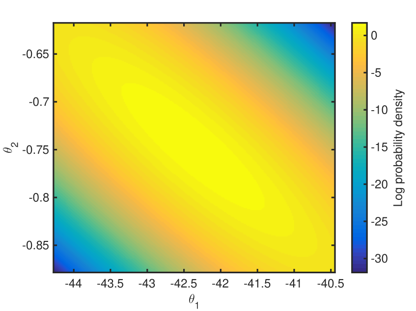
?figurename? 4: Plot of the log-likelihood of the Gaussian distribution of $\bm{\theta}$ in (20). $\bm{\Sigma}_{\theta}=\textbf{A}^{-1}$ is non-diagonal. A is computed in (25) from the FDR.

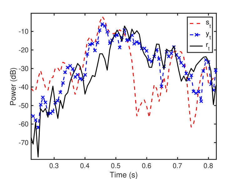
?figurename? 5: Plot of the true $s_{t}$, $y_{t}$ and the true $r_{t}$ at $1$ kHz when the noise type is white, $\text{SNR}=20$ dB, $T_{60}=0.68$ s and $\text{DRR}=-2.52$ dB.

The noisy reverberation, $z_{t}$, is the observation and, in this case, our aim is to find $r_{t}$ and $\Sigma_{t}^{(r)}$. We denote the noise floor in the power spectral domain by $|N|^{2}$. In a FDR, at high RNRs and when $|N|^{2}$ is low, we have $r_{t}\approx z_{t}$ because: $z=r+0.5\log(1+\text{RNR}^{-1}+2\cos(\zeta)\,\text{RNR}^{-0.5})$, which was also used in (13) and (14), where $\text{RNR}=\exp(2(r-n))$.

To solve the problem of finding $r_{t}$ and $\Sigma_{t}^{(r)}$ given the observed $z_{t}$, we first employ a minimum MSE (MMSE) algorithm, such as the traditional Log-MMSE estimator [43], to remove the noise and estimate the signal’s spectral amplitude, as in the end of Sec. 3.1 in [41], and then perform a KF update step and use $z_{t}$ as the KF observation. For the linear KF [44] [45], when the observation noise covariance matrix tends to zero at high RNRs, then the mean of the KF state goes to the KF observation and the variance of the KF state goes to zero. Therefore, a solution to finding $r_{t}$ and $\Sigma_{t}^{(r)}$ is to set $r_{t}=z_{t}$ and $\Sigma_{t}^{(r)}$ equal to a small value, such as $1$ $\text{dB}^{2}$.

The $T_{60}$ can be estimated from $\theta_{1}$ using $T_{60}=-\frac{3\log(10)}{\theta_{1}}$, where $\theta_{1}$ is computed from FDR data in the log-magnitude spectral domain [40]. The KF algorithm, which models $\gamma_{t}$ with a Gaussian distribution, uses a Gaussian prior for $\gamma$ with mean $L\mu_{\theta_{1}}$ and variance $L^{2}\Sigma_{\theta_{1}}$ because $\gamma=L\theta_{1}$. Using $\gamma=L\theta_{1}$, $\theta_{1}$ is directly mapped to $\gamma_{t}$, without going via the $T_{60}$.

The algorithm estimates a prior for $\beta$ directly, at the same time as the prior for $\gamma$, rather than first estimating the $T_{60}$ and the DRR. Figure 5 depicts $y_{t}$, $s_{t}$ and $r_{t}$ over time, at $1$ kHz, when the $T_{60}$ is $0.68$ s, the DRR is $-2.52$ dB, the noise type is white and the SNR is $20$ dB. In Fig. 5, $s_{t}$ and $r_{t}$ are the true speech and reverberation powers; the latter is computed by convolving the RIR without its first $30$ ms with the speech signal [2]. If we choose an appropriate FDR, then we can see that (1) is related to the FDR and the first frame of the FDR to the DRR. The $\beta$ reverberation parameter is computed from the difference between the log-amplitude of the first frame and the y-intercept of the LS fit, i.e. $\theta_{2}$. For the LS fit to the FDR, we choose to not use the first frame of the FDR. For the subtraction of two independent random variables, their means subtract and their variances add; $\theta_{2}$ has a mean and a variance and the log-amplitude of the first frame of the FDR has a mean and a fixed small variance. The prior for $\beta$ is given by

$$\beta=r_{t-M_{t}+C+1}-\theta_{2}\text{.}$$ (29)

We denote the mean of the internally computed Gaussian $\gamma_{t}$ prior by $\gamma_{t|t-1}^{\prime\prime}$ and its variance by $\Sigma_{t|t-1}^{(\gamma^{\prime\prime})}$. We use

$$\gamma_{t|t-1}=\dfrac{\gamma_{t|t-1}^{\prime}\Sigma_{t|t-1}^{(\gamma^{\prime\prime})}+\gamma_{t|t-1}^{\prime\prime}\Sigma_{t|t-1}^{(\gamma^{\prime})}}{\Sigma_{t|t-1}^{(\gamma^{\prime})}+\Sigma_{t|t-1}^{(\gamma^{\prime\prime})}}\text{,}$$ (30)

$$\Sigma_{t|t-1}^{(\gamma)}=\dfrac{\Sigma_{t|t-1}^{(\gamma^{\prime})}\Sigma_{t|t-1}^{(\gamma^{\prime\prime})}}{\Sigma_{t|t-1}^{(\gamma^{\prime})}+\Sigma_{t|t-1}^{(\gamma^{\prime\prime})}}\text{.}$$ (31)

Likewise, we denote the mean of the Gaussian $\beta_{t}$ prior by $\beta_{t|t-1}^{\prime\prime}$ and its variance by $\Sigma_{t|t-1}^{(\beta^{\prime\prime})}$. For $\beta_{t}$, we use

$$\beta_{t|t-1}=\dfrac{\beta_{t|t-1}^{\prime}\Sigma_{t|t-1}^{(\beta^{\prime\prime})}+\beta_{t|t-1}^{\prime\prime}\Sigma_{t|t-1}^{(\beta^{\prime})}}{\Sigma_{t|t-1}^{(\beta^{\prime})}+\Sigma_{t|t-1}^{(\beta^{\prime\prime})}}\text{,}$$ (32)

$$\Sigma_{t|t-1}^{(\beta)}=\dfrac{\Sigma_{t|t-1}^{(\beta^{\prime})}\Sigma_{t|t-1}^{(\beta^{\prime\prime})}}{\Sigma_{t|t-1}^{(\beta^{\prime})}+\Sigma_{t|t-1}^{(\beta^{\prime\prime})}}\text{.}$$ (33)

Assuming that the RIR is known, it is straightforward to compute the $T_{60}$: compute the energy decay curve, plot it on a log scale and estimate the $T_{60}$ from its slope. On the contrary, estimating the $T_{60}$ blindly is not trivial. The KF algorithm estimates the $T_{60}$, applying internally estimated priors using the decay rate of the LS fit to the FDR [40], so that the KF does not diverge and does not treat reverberation as speech.

III-E The Peripheral Blocks of the Algorithm

This section describes the unshaded peripheral blocks of the KF algorithm in Fig. 3. The algorithm uses pre-cleaning before performing speech AR modelling, as in [33] and [45]. Pre-cleaning has also been used in [46] [47], in [11] [34] and in [10] [48]. The “Speech pre-cleaning” block in Fig. 3 affects the “Speech KF prediction” block and not the observation of the non-linear “KF Update” block, i.e. $y_{t}$, used in step 7.

For the “Noise power estimation” block, an external noise power estimator, such as [49], is used. External noise estimation and log-normal noise power modelling, as in [50] [51], are used for $n_{t|-}$, which is then used in step 6 of Table I.

In summary, the KF algorithm tracks speech and reverberation in the spectral log-magnitude domain along with $\gamma_{t}$ and $\beta_{t}$, as described in Fig. 3 and in the signal model in Fig. 2.

IV Implementation, Testing and Validation

We use acoustic frames of length $32$ ms and an acoustic frame increment of $L=8$ ms in (2). We also use modulation frames of $64$ ms and a modulation frame increment of $8$ ms [33] [34]. In Fig. 3, for speech amplitude spectrum pre-cleaning, we use the Log-MMSE estimator [43] followed by the WPE dereverberation algorithm [52] [53]. The dimension of the speech KF state, $\textbf{s}_{t}$, in (6) is $p=2$. In the “Noise power estimation” block of Fig. 3, we use external noise power estimation from [49] using the implementation in [54].

The outer integrals in Secs. III.B and III.C are performed using sigma points, as in [33]. The numbers of sigma points used in (11)-(17) are $K_{(\delta,\epsilon)}=K_{(r,n)}=K_{z_{t|t}}=K_{r_{t|t}}=3$ and $K_{\eta}=K_{\zeta}=K_{\lambda}=K_{\iota}=K_{\xi}=6$. For the latter cases, for $\xi$, the sigma points are at $\xi=((1:K_{\xi})-0.5)\frac{\pi}{K_{\xi}}$ and the weights are all equal to $\frac{1}{K_{\xi}}$ [33] [32]. With this choice of sigma points for $\xi$, the integral will be exact for an integrand that is a sum of terms of the form $\cos(n\xi)$ for $0\leq n\leq 2K_{\xi}+1$.

In Sec. III.D, for the $\gamma_{t}$ and $\beta_{t}$ priors, the look-ahead factor is $C=3$ frames. For the FDR that is comprised of frames with decreasing energy, $M_{t}$ is computed in every frame.

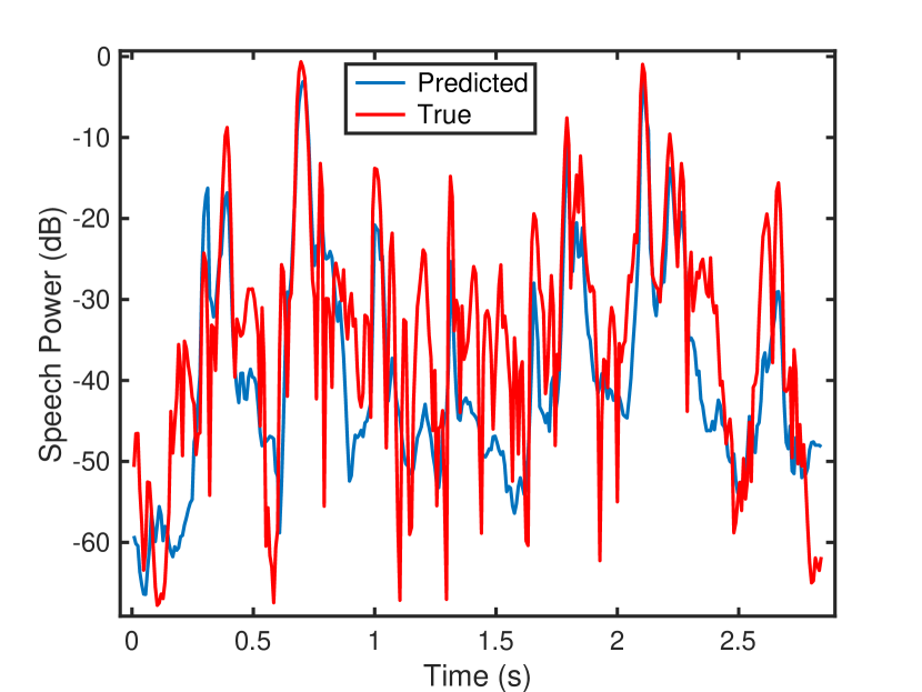
(a)

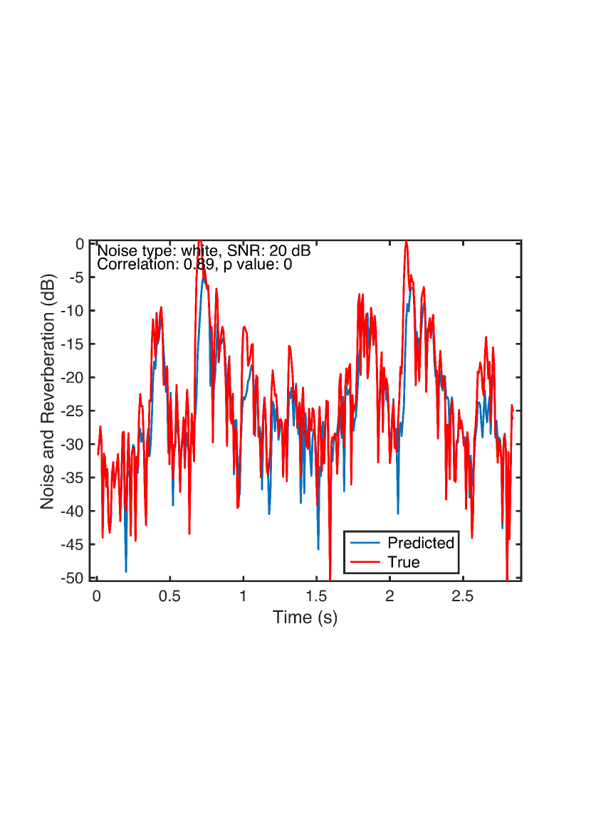
(b)

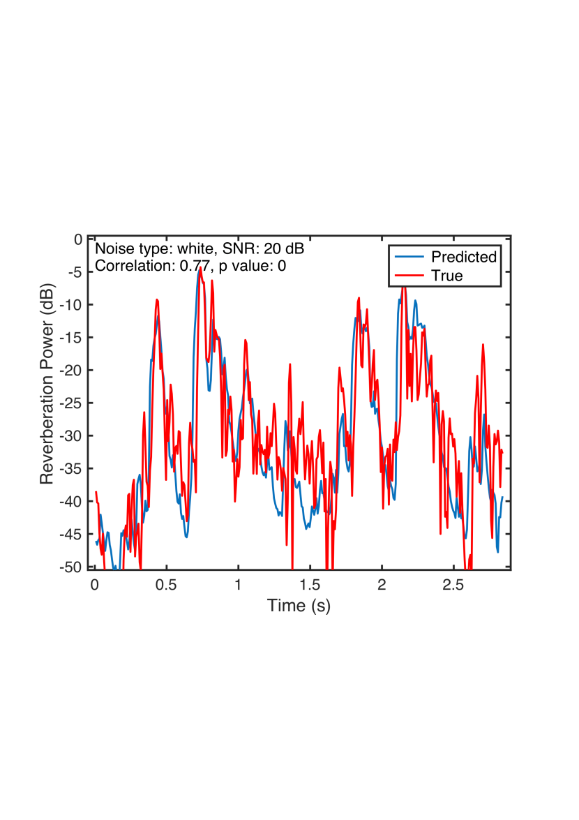
(c)

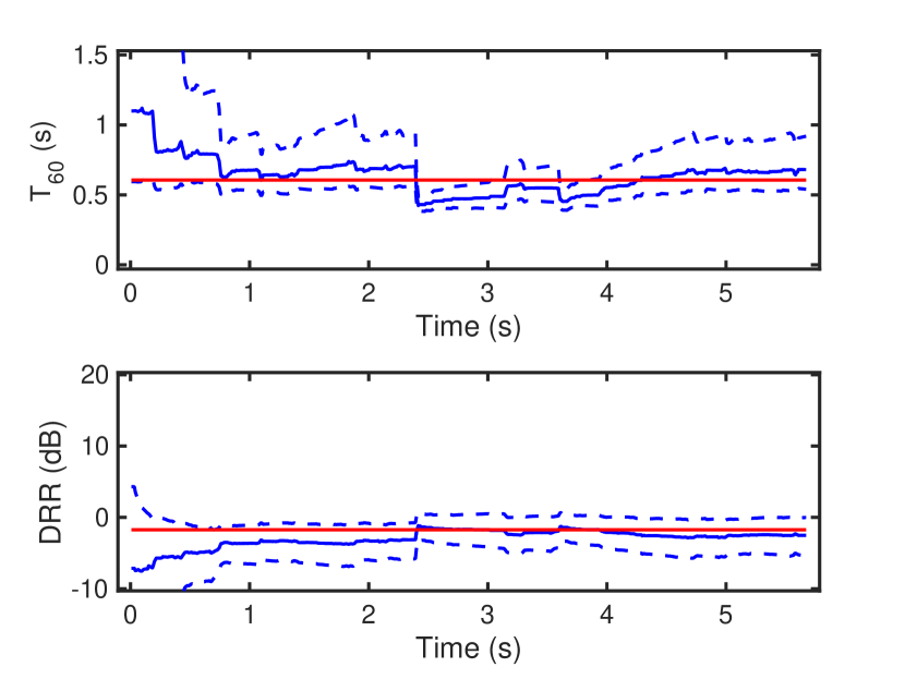
(d)

?figurename? 6: Plot of the predicted and true: (a) speech power, i.e. $s_{t|t}$ and the true $s_{t}$, at $1$ kHz, (b) noise and reverberation power, i.e. $z_{t|t}$ and the true $z_{t}$, at $1$ kHz, (c) reverberation power, i.e. $r_{t|t}$ and the true $r_{t}$, at $1$ kHz, and (d) $T_{60}$ and DRR reverberation parameters. In (a)-(d), the $T_{60}$ is $0.61$ s and the DRR is $-1.74$ dB, while the noise type is white and the SNR is $20$ dB.

Figures 6(a)-(c) illustrate $s_{t}$, $z_{t}$ and $r_{t}$ at $1$ kHz over time, as Fig. 3 in [45]. Figure 6(a) shows the predicted and true speech power, i.e. $s_{t|t}$ and the true $s_{t}$, and Fig. 6(b) the predicted and true noise and reverberation power, i.e. $z_{t|t}$ and the true $z_{t}$. The correlation coefficient between the true $z_{t}$ and $z_{t|t}$ is $0.89$. Figure 6(c) shows the predicted and true reverberation power, i.e. $r_{t|t}$ and the true $r_{t}$. The correlation coefficient between the true $r_{t}$ and $r_{t|t}$ is $0.77$ $(<0.89)$. The noise type is white, the SNR is $20$ dB, $T_{60}=0.61$ s and $\text{DRR}=-1.74$ dB.

The ordering of the graphs in Figs. 6(a)-(c) matches the ordering of the signal decompositions in the KF algorithm, in Table LABEL:tab:ppssaaa. The noisy reverberant observation is first decomposed into $s_{t}$ and $z_{t}$ with step 7 in Table LABEL:tab:ppssaaa; Figs. 6(a) and (b) illustrate $s_{t|t}$ and $z_{t|t}$, respectively, over time. Then, $z_{t|t}$ is decomposed into $r_{t}$ and $n_{t}$ with step 8; Fig. 6(c) depicts $r_{t|t}$ over time.

?tablename? I: List of the environments sorted with respect to the $T_{60}$ from A to I and from J to V. The room dimensions are $5\times 4\times 4$ or $10\times 7\times 3$ m. The source-microphone distance is $1.5$ m. The wall reflection coefficient is adjusted to vary the $T_{60}$ and the DRR. For $a$ and $b$ in (2), $L=8$ ms.

Index	$T_{60}$ (s)	DRR (dB)	Room (m$\times$m$\times$m)	$a$	$b$
A	$0.18$	$8.43$	$5\times 4\times 4$	$0.54$	$0.07$
B	$0.25$	$5.78$	$5\times 4\times 4$	$0.64$	$0.10$
C	$0.33$	$3.13$	$5\times 4\times 4$	$0.72$	$0.14$
D	$0.40$	$1.69$	$5\times 4\times 4$	$0.76$	$0.16$
E	$0.47$	$0.25$	$5\times 4\times 4$	$0.79$	$0.20$
F	$0.54$	$-0.74$	$5\times 4\times 4$	$0.81$	$0.23$
G	$0.61$	$-1.74$	$5\times 4\times 4$	$0.83$	$0.25$
H	$0.64$	$-2.13$	$5\times 4\times 4$	$0.84$	$0.26$
I	$0.68$	$-2.52$	$5\times 4\times 4$	$0.85$	$0.27$
J	$0.21$	$8.07$	$10\times 7\times 3$	$0.59$	$0.06$
K	$0.31$	$2.74$	$10\times 7\times 3$	$0.70$	$0.16$
L	$0.40$	$0.17$	$10\times 7\times 3$	$0.76$	$0.23$
M	$0.50$	$0.11$	$10\times 7\times 3$	$0.80$	$0.19$
N	$0.59$	$-0.73$	$10\times 7\times 3$	$0.83$	$0.20$
O	$0.64$	$-0.95$	$10\times 7\times 3$	$0.84$	$0.20$
P	$0.69$	$-1.12$	$10\times 7\times 3$	$0.85$	$0.19$
Q	$0.71$	$-1.68$	$10\times 7\times 3$	$0.86$	$0.21$
R	$0.73$	$-2.01$	$10\times 7\times 3$	$0.86$	$0.22$
S	$0.85$	$-2.09$	$10\times 7\times 3$	$0.88$	$0.19$
T	$0.97$	$-2.95$	$10\times 7\times 3$	$0.89$	$0.22$
U	$1.01$	$-3.11$	$10\times 7\times 3$	$0.90$	$0.20$
V	$1.05$	$-3.33$	$10\times 7\times 3$	$0.90$	$0.22$

The $T_{60}$ and DRR estimates should converge to their true constant values when the talker and the microphone are not moving and the frequency variations in the reflection coefficients are not modelled [55] [56]. Internally estimated priors for $\gamma_{t}$ and $\beta_{t}$ make the reverberation parameters converge over time. Figure 6(d) shows the predicted and true $T_{60}$ and DRR reverberation parameters over time. The dashed lines are the signals’ standard deviations, computed from $\gamma_{t}$ and $\beta_{t}$.

V Evaluation of the Algorithm

The proposed KF algorithm is evaluated in terms of the perceptual evaluation of speech quality (PESQ) [57], the cepstral distance (CD) spectral divergence metric [58], the reverberation decay tail (RDT) dereverberation metric [59] and the STOI speech intelligibility metric [60] [61]. The ideal values of CD and RDT, which have been also used in [18], are zero. For evaluation, the TIMIT database [62], sampled at $16$ kHz, and the RSG-10 noise database [63] are used. From the TIMIT database, $52$ clean speech utterances are chosen. We use artificially-created reverberation with the image method [55] using the implementation in [64]. The wall reflection coefficient is adjusted to vary the $T_{60}$ and hence also the DRR. The KF algorithm is evaluated with noisy reverberant speech signals at various SNRs, from $5$ to $20$ dB, using random noise segments and the noise types of white, babble and factory.

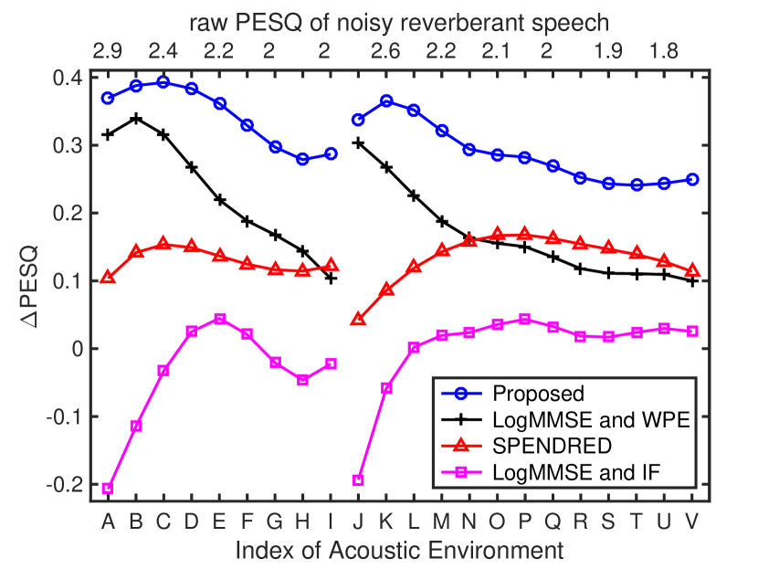
(a)

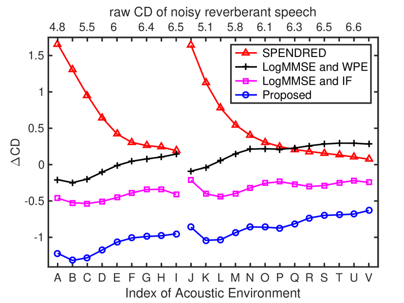
(b)

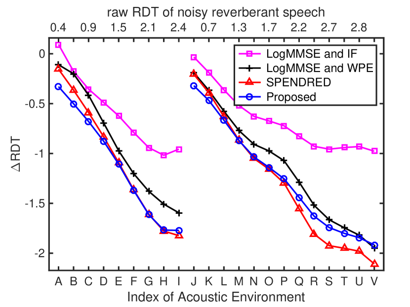
(c)

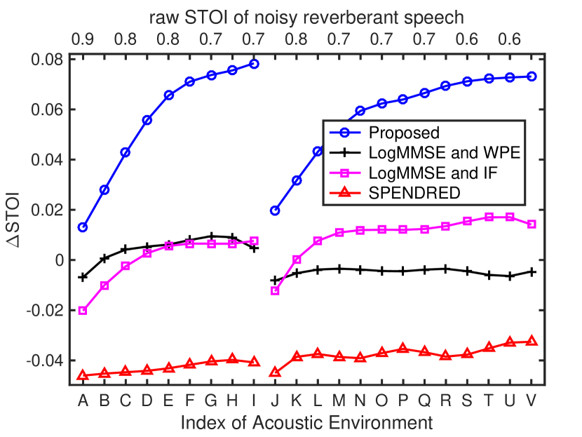
(d)

?figurename? 7: Plot of: (a) $\Delta$PESQ where higher scores signify better speech quality, (b) $\Delta$CD where lower values signify better speech quality, (c) $\Delta$RDT where lower values signify better dereverberation, and (d) $\Delta$STOI where higher scores signify better intelligibility. The graphs are against the index of the acoustic environment and, hence, against the $T_{60}$ and the DRR. The mean over the noises of white, babble and factory at $20$ dB SNR is shown.

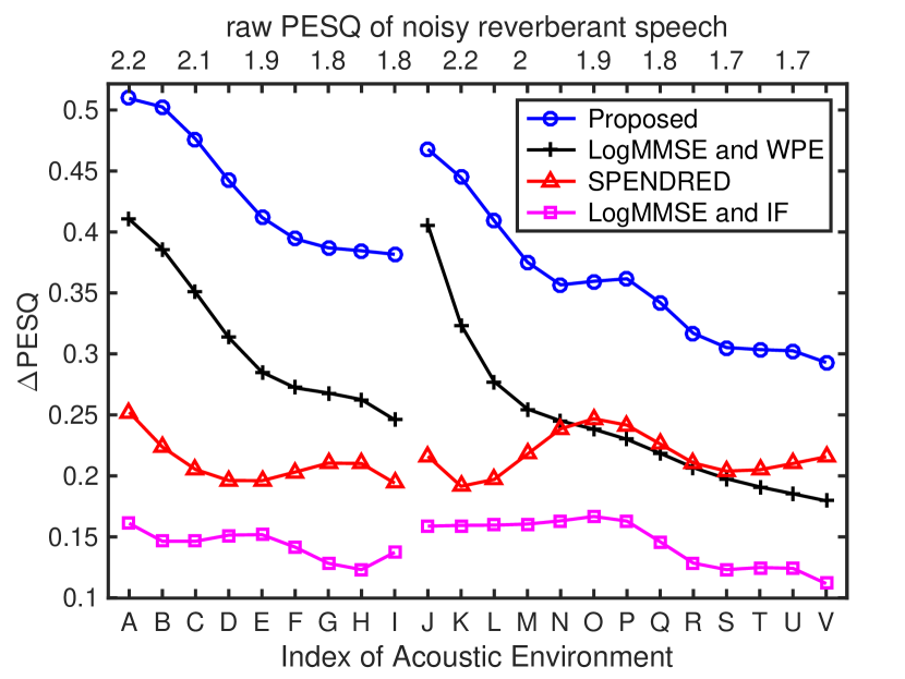
(a)

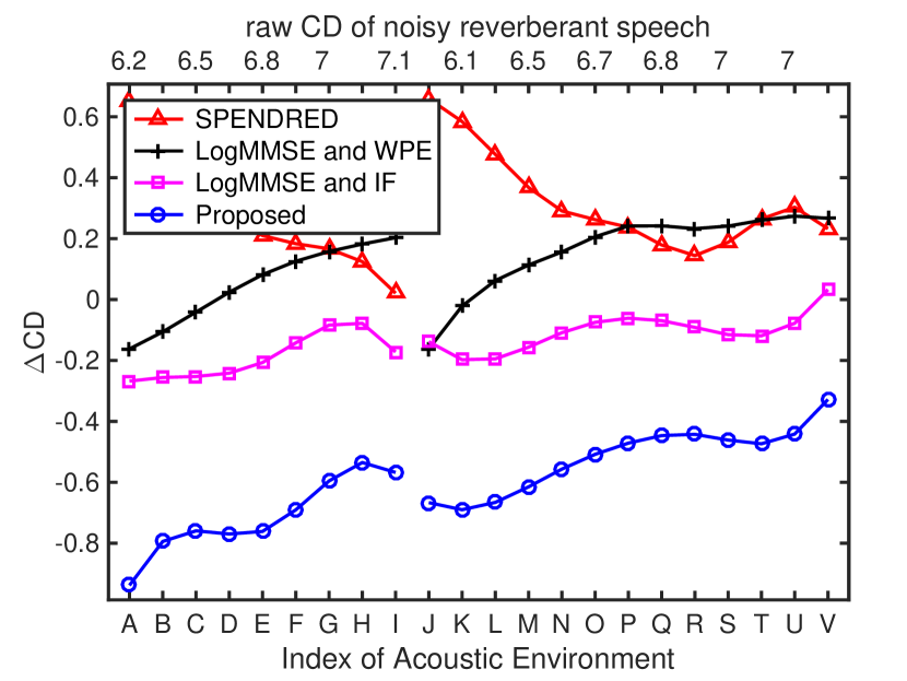
(b)

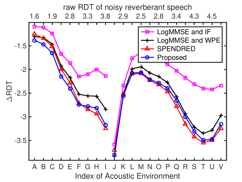
(c)

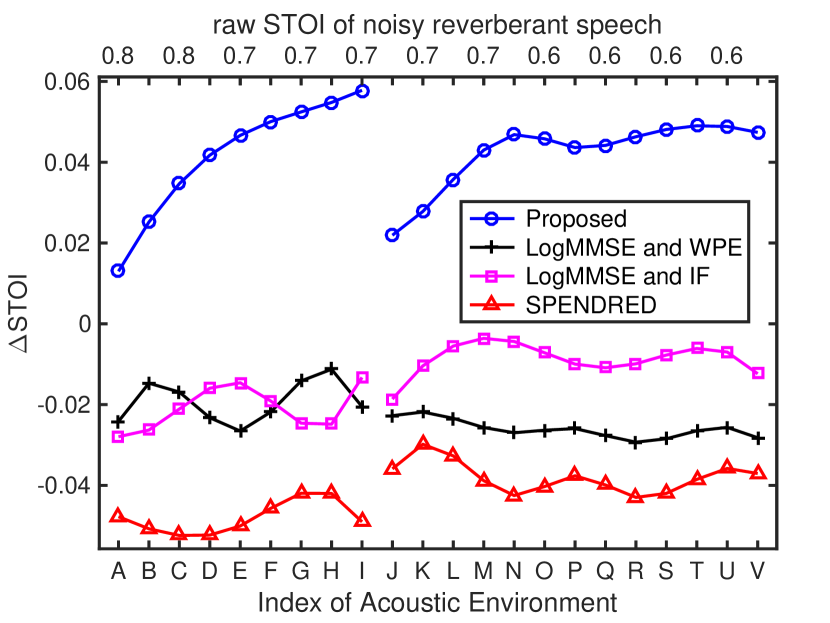
(d)

?figurename? 8: Plot of: (a) $\Delta$PESQ, (b) $\Delta$CD, (c) $\Delta$RDT, and (d) $\Delta$STOI. The graphs are against the index of the acoustic environment. The average over the noise types of white, babble and factory at $10$ dB SNR is shown.

The KF algorithm is compared to the SPENDRED algorithm [18] [19], which jointly performs blind denoising and dereverberation, and to algorithms that sequentially perform denoising and dereverberation, specifically to the Log-MMSE estimator [43] followed by the WPE algorithm [53] [30] and to the Log-MMSE estimator followed by an inverse-filter (IF) dereverberation method that is based on $T_{60}$ and DRR estimates [41]. For the IF, we blindly estimate the $T_{60}$ and the DRR for the entire speech utterance using the algorithm in [41] [65], whose implementation was generously provided by the author. As found in the Acoustic Characterisation of Environments (ACE) challenge [1], the $T_{60}$ estimator in [41] had the best performance of the examined $T_{60}$ estimators.

For evaluation, the examined acoustic conditions are shown in Table I. Two different rooms with dimensions $5\times 4\times 4$ m and $10\times 7\times 3$ m are used. The distance between the microphone and the talker is $1.5$ m. Table I is sorted with respect to the $T_{60}$ and the DRR from A to I and from J to V. We plot the improvement in PESQ, $\Delta$PESQ, against the index of the acoustic environment to evaluate the KF algorithm. The top axis shows the raw PESQ of the noisy reverberant speech and is monotonic from A to I and from J to V. Similar graphs are also plotted for the other metrics. The ordering of the legends matches that of the algorithms at low $T_{60}$ values.

Table I also shows the $a$ and $b$ reverberation values of the RIRs and we note that one of the baselines that we use, i.e. the SPENDRED algorithm [18] [19], assumes that $b\leq 1$. This is valid in Table I because $b<<1$ and its range is small.

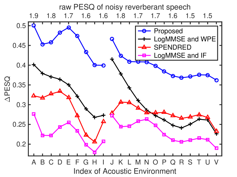
(a)

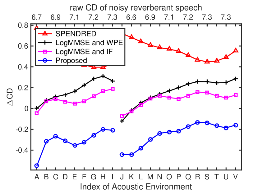
(b)

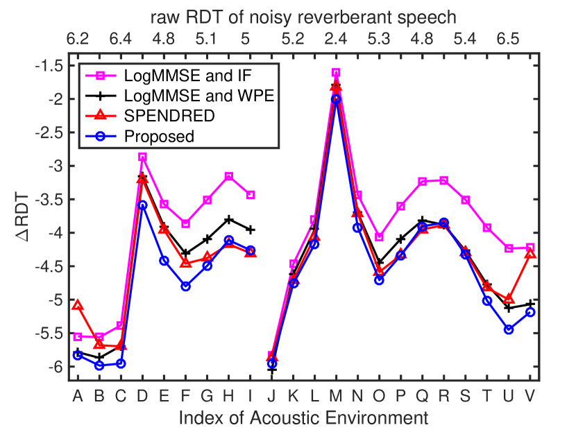
(c)

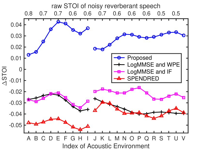
(d)

?figurename? 9: Plot of: (a) $\Delta$PESQ, (b) $\Delta$CD, (c) $\Delta$RDT, and (d) $\Delta$STOI. The graphs are against the index of the acoustic environment. The average over the noise types of white, babble and factory at $5$ dB SNR is shown.

V-A Overall Performance Against the $T_{60}$ and the DRR

This section investigates the overall performance of the KF algorithm against the $T_{60}$ and the DRR. Figure 7 examines: (a) the $\Delta$PESQ, where higher scores signify better speech quality, (b) the $\Delta$CD, where lower values signify better speech quality, (c) the $\Delta$RDT, where lower values signify better dereverberation, and (d) the $\Delta$STOI, where higher scores signify better intelligibility. Figure 7 first presents the results that are related to speech quality, in (a) and (b). Then, it shows the dereverberation results, in (c), and the speech intelligibility results, in (d). The graphs are against the index of the acoustic environment and, hence, against the $T_{60}$ and the DRR. The average over the noise types of white, babble and factory at $20$ dB SNR is shown. We note that noisy reverberant speech with $T_{60}\approx 0.6$ s has a raw PESQ score of $2$ in Fig. 7(a).

In Fig. 7(a), the top axis is monotonic from A to I and from J to V and there is no transition from index I to index J.

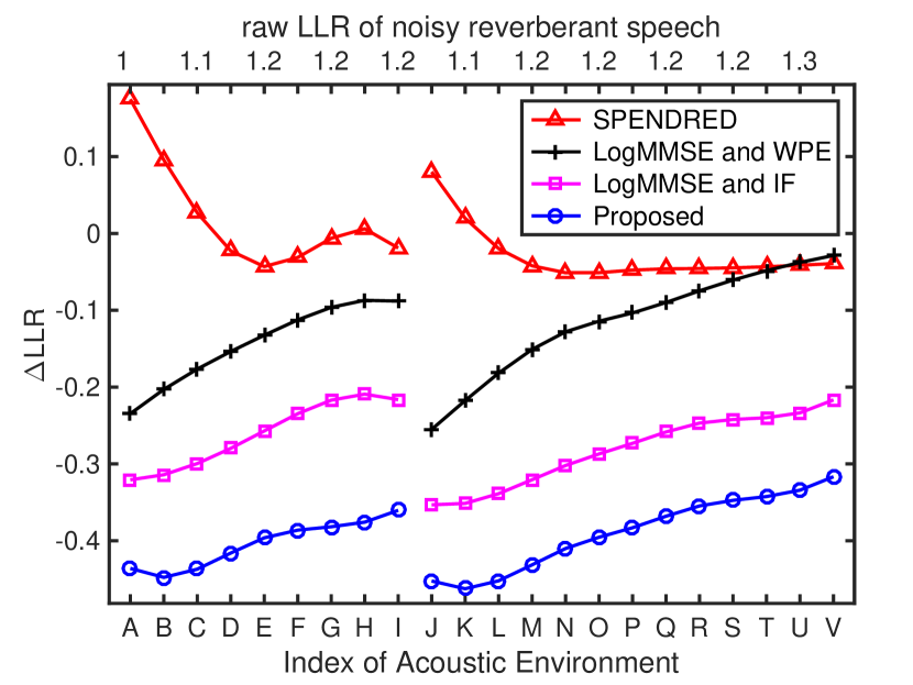
(a)

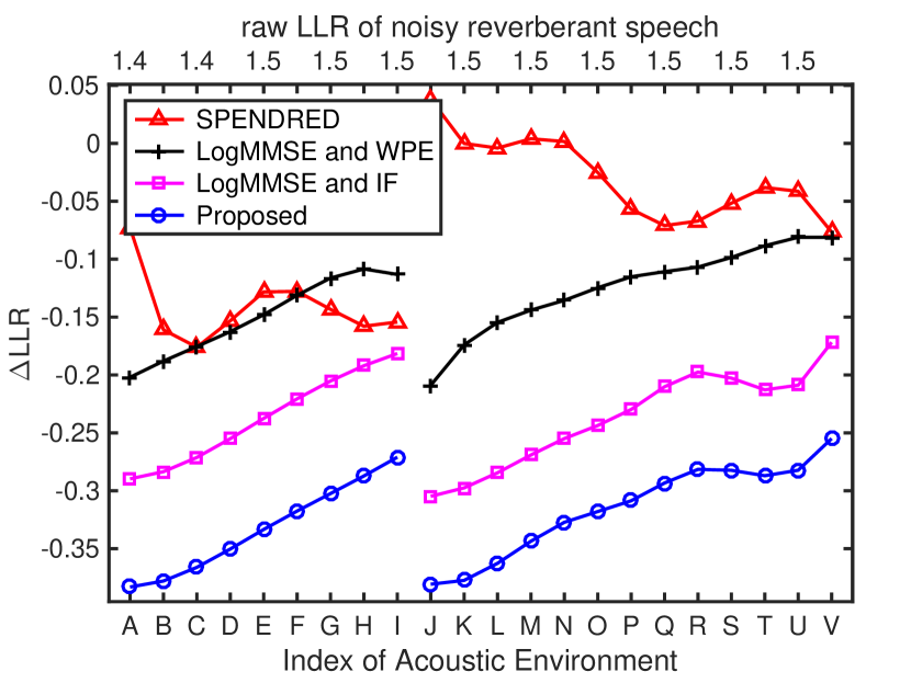
(b)

?figurename? 10: Plot of $\Delta$LLR where lower scores signify better speech quality when white noise is used: (a) at $20$ dB SNR, and (b) at $10$ dB SNR.

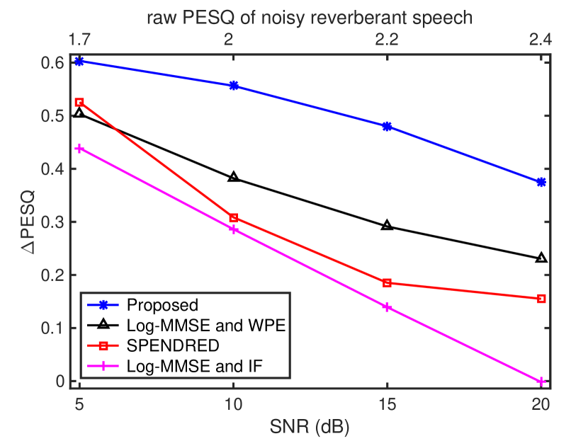
(a)

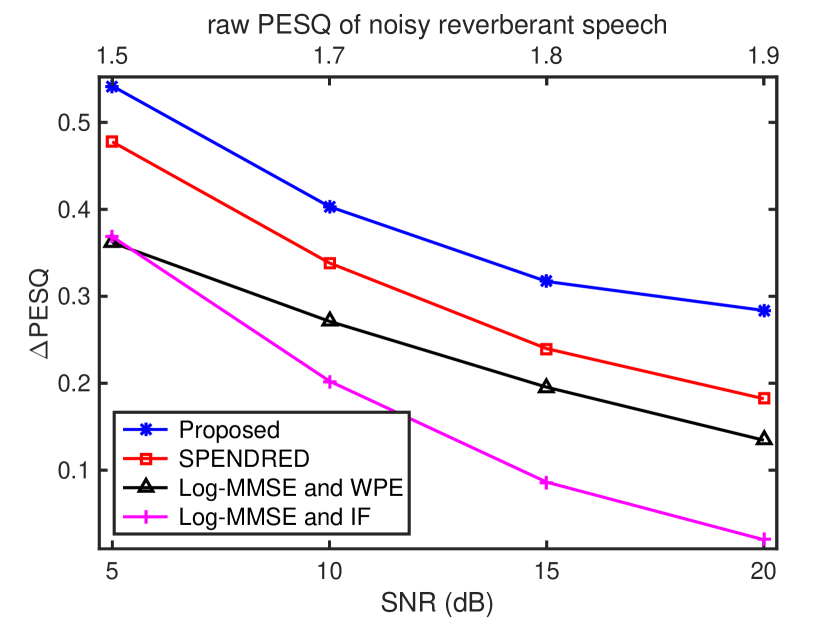
(b)

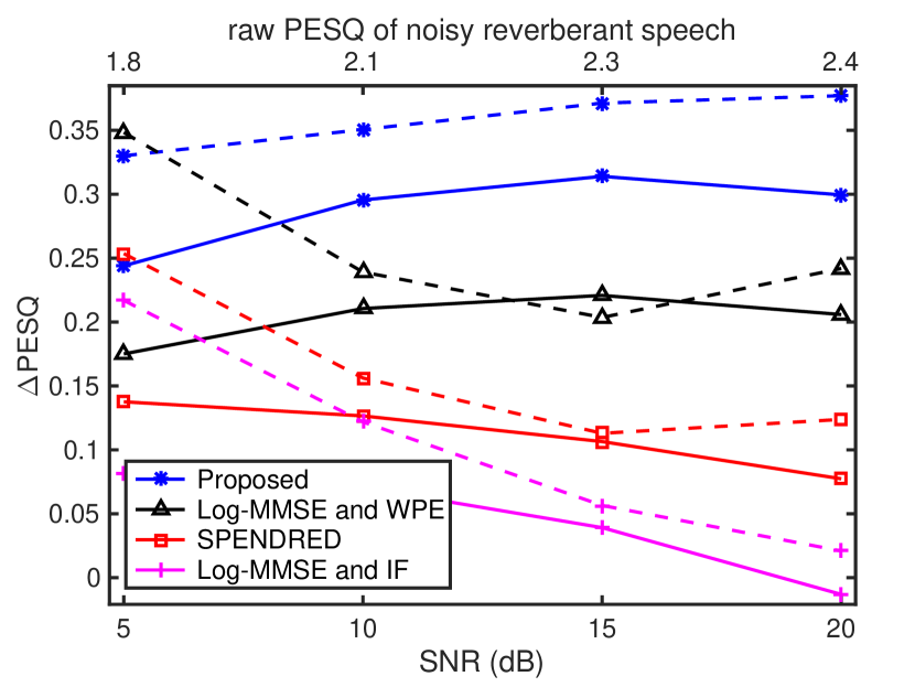
(c)

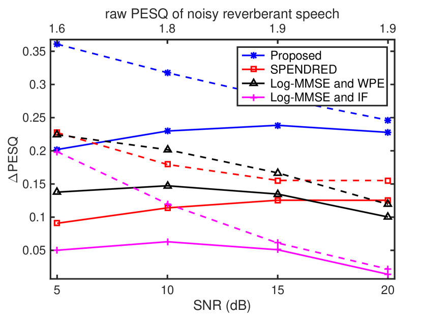
(d)

?figurename? 11: Plot of $\Delta$PESQ against SNR for: (a), (b) white noise, and (c), (d) babble noise (solid lines) and factory noise (dashed lines). In (a) and (c), $T_{60}=0.40$ s and DRR = 0.17 dB (i.e. index L in Table I). In (b) and (d), $T_{60}=0.73$ s and DRR = -2.1 dB (i.e. index R). In (c) and (d), babble noise is used for the top axis and for the legends.

From Fig. 7(a), in terms of PESQ, the proposed algorithm consistently yields improved speech quality in challenging environments compared to the examined baselines. Compared to the unprocessed noisy reverberant speech, the algorithm shows improved performance for all the examined $T_{60}$ range from $0.18$ to $1.05$ s and DRR range from $8.43$ to $-3.33$ dB. Compared to the unprocessed speech, for a $T_{60}$ of $0.3$ and $1$ s, the algorithm has a $\Delta$PESQ of $0.35$ and $0.25$, respectively, for the SNR of $20$ dB averaged over the examined noises.

From Fig. 7(b), in terms of CD, the KF algorithm yields improved speech quality in acoustic environments with a $T_{60}$ from $0.18$ to $1.05$ s. The KF algorithm shows a deteriorating CD improvement with increasing $T_{60}$. Compared to the unprocessed signal, for a $T_{60}$ of $0.3$ and $1$ s, the algorithm has a CD improvement of approximately $-1.1$ and $-0.6$, respectively, for the SNR of $20$ dB averaged over the tested noise types.

From Fig. 7(c), we observe that the KF algorithm yields improved speech dereverberation in challenging acoustic conditions and that the $\Delta$RDT improves with increasing $T_{60}$ values. From the raw RDT of noisy reverberant speech in Fig. 7(c), we observe that the indexes A and J have very low reverberation. The indexes A and J have raw RDT scores $0.4$ and $0.7$, respectively. The indexes G-I and T-V have high reverberation with a high raw RDT score. The proposed algorithm in these high reverberation cases achieves a large RDT improvement decreasing the RDT metric from approximately $2.6$ to $0.8$.

From Fig. 7(d), the KF algorithm shows marginally improved STOI performance for the examined $T_{60}$ range compared to the unprocessed speech and to the examined baselines. For a $T_{60}$ of $0.3$ and $1$ s, the algorithm has a $\Delta$STOI of $0.03$ and $0.07$, respectively. With increasing $T_{60}$, the $\Delta$STOI scores slightly increase. The baselines have negative $\Delta$STOI.

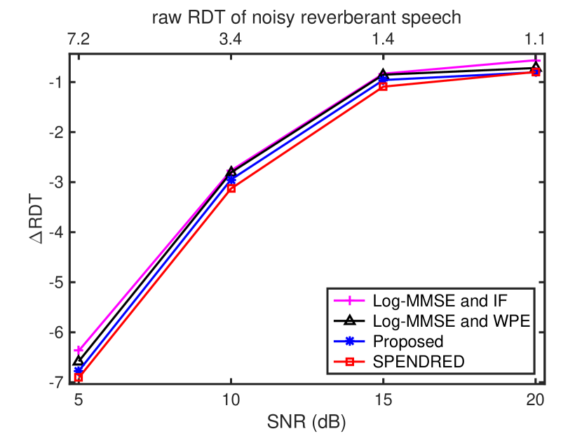
(a)

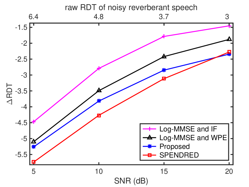
(b)

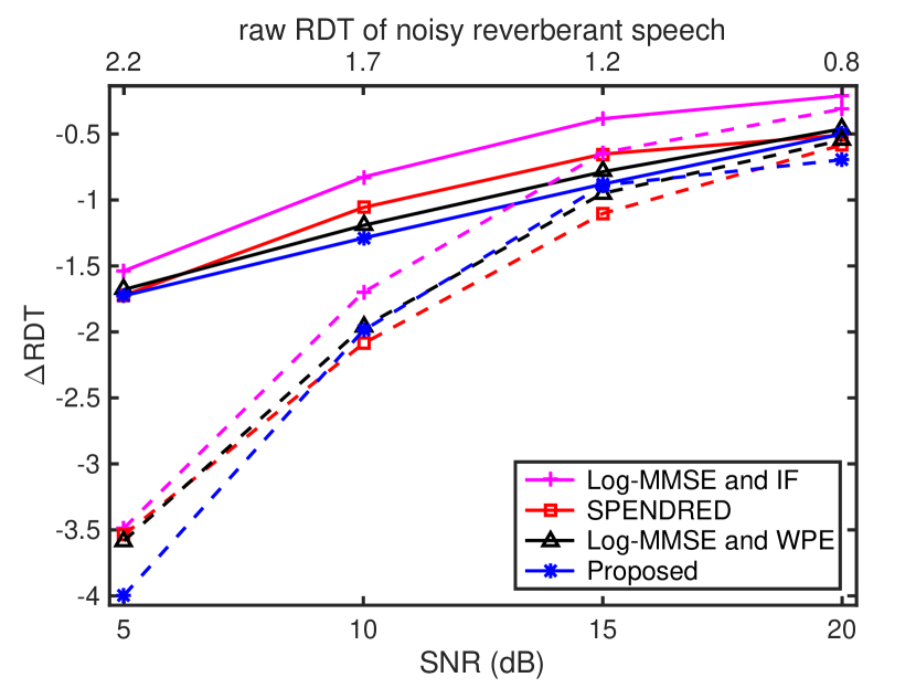
(c)

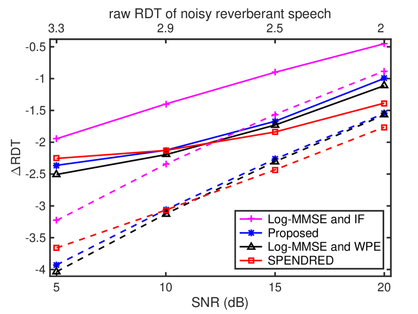
(d)

?figurename? 12: Plot of $\Delta$RDT against SNR for: (a), (b) white noise, and (c), (d) babble noise (solid lines) and factory noise (dashed lines). In (a) and (c), $T_{60}=0.40$ s and DRR = 0.17 dB (i.e. index L in Table I). In (b) and (d), $T_{60}=0.73$ s and DRR = -2.1 dB (i.e. index R). In (c) and (d), babble noise is used for the top axis and for the legends.

We use the noise types of white, babble and factory at $10$ dB SNR and we obtain Fig. 8. Figure 8 shows similar graphs to Fig. 7 but for a SNR of $10$ dB. For all the examined $T_{60}$ values, the KF algorithm shows a consistent improvement in the evaluation metrics of PESQ, CD, RDT and STOI.

We now use the noise types of white, babble and factory at $5$ dB SNR and we obtain Fig. 9. Figure 9 shows similar graphs to Figs. 7 and 8. For all the examined SNRs, the KF algorithm shows a consistent improvement in the examined metrics, depending on the $T_{60}$. From Fig. 9(a), we observe that the $\Delta$PESQ scores of the KF algorithm at $5$ dB SNR are similar to the $\Delta$PESQ scores at $10$ dB SNR in Fig. 8(a).

The KF algorithm shows improved PESQ performance for the examined SNRs from $5$ dB to $20$ dB. The algorithm has better speech quality performance compared to the baselines for all the examined $T_{60}$ values. Compared to the unprocessed noisy reverberant speech, for the SNR of $5$ dB, the algorithm has a $\Delta$PESQ of about $0.45$ for a $T_{60}$ of $0.6$ s and a raw PESQ of $1.6$. For the SNR of $20$ dB, the algorithm has a $\Delta$PESQ of approximately $0.3$ for a $T_{60}$ of $0.6$ s and a raw PESQ of $2$. Comparing Figs. 7-9, we observe that the raw PESQ decreases with decreasing SNR while the $\Delta$PESQ increases.

The KF algorithm yields improved dereverberation performance in terms of RDT in adverse conditions in Fig. 9(c). The algorithm’s performance improves with decreasing SNR. We observe that the indexes A-C and J-K have a high raw RDT despite that they have low reverberation at $5$ dB SNR, when the effect of noise is higher than that of reverberation.

The results of the log-likelihood ratio (LLR) speech quality metric [66] [67], which is used as the main evaluation metric in the dereverberation algorithm in [68], resemble the results of CD in Fig. 10. Both CD and LLR have been used in the REVERB challenge [4] [3]. It was found in [67] that LLR correlates well with speech quality although slightly less well than PESQ. Figure 10 examines $\Delta$LLR when white noise is used at $20$ and $10$ dB SNR. From Fig. 10, we observe that decreasing the SNR from $20$ to $10$ dB increases the raw LLR of noisy reverberant speech and deteriorates the $\Delta$LLR.

V-B Overall Performance Against the SNR

This section investigates the overall performance of the KF algorithm against the SNR. Figure 11 presents the algorithm’s PESQ performance compared to the baselines. Figures 11(a) and 11(b) depict the PESQ improvement, $\Delta$PESQ, against the SNR for white noise when: (a) $T_{60}=0.40$ s and DRR = 0.17 dB, which is case L in Table I, and (b) $T_{60}=0.73$ s and DRR = -2.1 dB, which is case R in Table I. The indexes L and R were chosen because they are not extreme cases and they have different $T_{60}$ and DRR values. The ordering of the legends in Fig. 11 matches that of the algorithms at high SNRs.

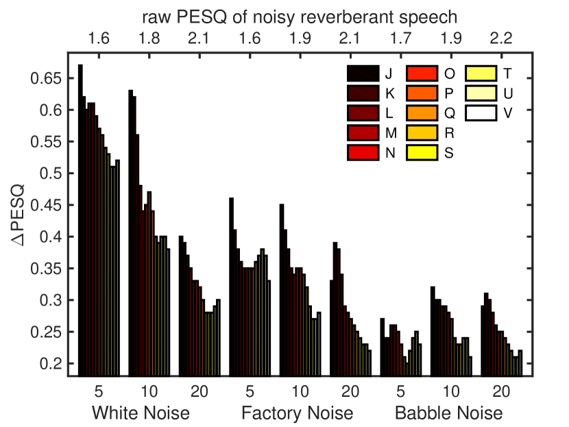
(a)

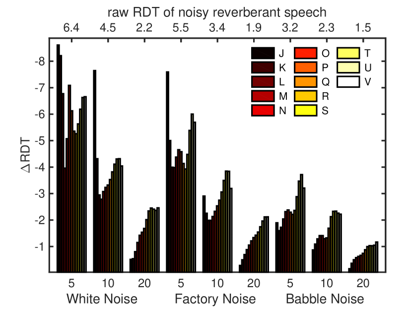
(b)

?figurename? 13: Plot of (a) $\Delta$PESQ, and (b) $\Delta$RDT against SNR (dB) for the KF algorithm for white, factory and babble noises. The indexes J to V are shown.

Figures 11(c) and 11(d) show the $\Delta$PESQ against the SNR for babble and factory noises, for cases L and R in Table I respectively, for the KF algorithm compared to the baselines. Babble noise is used for the solid lines, the top axis and the legends while factory noise is used for the dashed lines. The KF algorithm has a $\Delta$PESQ that is dependent on the SNR and noise type and is, most of the times, increasing with decreasing SNRs. Compared to the unprocessed speech in Fig. 11(c), the algorithm has a $\Delta$PESQ of about $0.35$ for factory noise for SNRs from $5$ to $20$ dB, while decreasing for lower SNRs.

Figure 12 examines the RDT improvement, $\Delta$RDT, against the SNR for white noise, for cases L and R in Table I, in (a) and (b). Figure 12 also depicts the $\Delta$RDT against the SNR for babble and factory noises, for cases L and R in Table I, in (c) and (d). Babble noise is used for the solid lines, the top axis and the legends. Factory noise is used for the dashed lines. Figures 12(a)-(d) show that the $\Delta$RDT improves and the raw RDT of noisy reverberant speech increases with decreasing SNR. The $\Delta$RDT scores are better for stationary white noise than for non-stationary factory and babble noises.

Figure 13 shows the $\Delta$PESQ and the $\Delta$RDT against the SNR, from $5$ to $20$ dB, for the KF algorithm for white, factory and babble noises. Figure 13 examines the acoustic conditions J to V that correspond to the room $10\times 7\times 3$ m in Table I. Figure 13 differs from Figs. 11 and 12 in presenting the indexes J to V and not only L and R. From Fig. 13(a), we observe that the $\Delta$PESQ decreases as the $T_{60}$ increases. The $\Delta$PESQ improves with decreasing SNR and the $\Delta$PESQ is higher for white noise than for factory and babble noises. In Fig. 13(b), the $\Delta$RDT improves as the $T_{60}$ increases and, moreover, the $\Delta$RDT improves with decreasing SNR.

In summary, in this evaluation section, we have tested the KF algorithm in different SNRs, noise types and acoustic conditions with different $T_{60}$ and DRR values. The algorithm is effective in enhancing distorted speech, decomposing noisy reverberant speech into speech, reverberation and noise. Regarding noise robustness, Figs. 7-13 show that the proposed KF algorithm achieves a significant performance gain over different noise types and SNRs, compared to the unprocessed noisy reverberant speech and to the examined baselines.

VI Conclusion

In this paper, we present a monaural speech enhancement algorithm based on Kalman filtering in the log-magnitude spectral domain to blindly suppress noise and reverberation while accounting for inter-frame speech dynamics. The first two moments of the posterior distribution of the speech log-magnitude spectrum are estimated in noisy reverberant environments using a model that adaptively updates the $T_{60}$ and DRR reverberation parameters. The non-linear KF algorithm updates and tracks the two reverberation parameters of $\gamma_{t}$ and $\beta_{t}$ to further improve the estimation of the speech log-magnitude spectrum. In this paper, we show by means of theoretical and experimental analyses that Kalman filtering can be performed in challenging conditions by performing the proposed signal decompositions into speech, reverberation and noise, propagating backwards through the proposed signal model. Experimental results using instrumental measures show improved performance against both the $T_{60}$ and the SNR compared to the unprocessed noisy reverberant speech and to alternative competing techniques that perform blind denoising and dereverberation either in concatenation or jointly.

References

- [1] J. Eaton, N. D. Gaubitch, A. H. Moore and P. A. Naylor, “Estimation of room acoustic parameters: The ACE challenge,” IEEE Trans. on Audio, Speech and Language Process., vol. 24, no. 10, pp. 1681-1693, Oct. 2016.
- [2] J. Li and L. Deng and R. Haeb-Umbach and Y. Gong, Robust automatic speech recognition: A bridge to practical applications, Ch. 9: Reverberant speech recognition. Elsevier, ISBN: 978-0-12-802398-3, 2016.
- [3] K. Kinoshita, M. Delcroix, S. Gannot, E. Habets et al., “A summary of the REVERB challenge: State-of-the-art and remaining challenges in reverberant speech processing research,” EURASIP J. Adv. Signal Process., vol. 7, pp. 1-19, 2016.
- [4] K. Kinoshita, M. Delcroix, T. Yoshioka, T. Nakatani, E. Habets et al., “The REVERB challenge: A common evaluation framework for dereverberation and recognition of reverberant speech,” in Proc. IEEE Workshop on Applications of Signal Processing to Audio and Acoustics, New Paltz, NY, Oct. 2013.
- [5] C. S. J. Doire, M. Brookes, P. A. Naylor, D. Betts, C. M. Hicks, M. A. Dmour and S. H. Jensen, “Single-channel blind estimation of reverberation parameters,” in Proc. IEEE Intl. Conf. on Acoustics, Speech and Signal Processing, Brisbane, Australia, pp. 31-35, April 2015.
- [6] K. Lebart, J. M. Boucher, and P. N. Denbigh, “A New Method Based on Spectral Subtraction for Speech Dereverberation,” Acta Acoustica, vol. 87, pp. 359–366, 2001.
- [7] S. O. Sadjadi and J. H. L. Hansen, “Blind spectral weighting for robust speaker identification under reverberation mismatch,” IEEE Trans. on Audio, Speech and Language Process., vol. 22, no. 5, pp. 937-945, May 2014.
- [8] I. J. Tashev, Sound Capture and Processing, Ch. 8: De-reverberation. John Wiley and Sons, ISBN: 978-0-470-31983-3, Aug. 2009.
- [9] E. A. P. Habets, “Single- and Multi-Microphone Speech Dereverberation using Spectral Enhancement, Ch. 6: Late Reverberant Spectral Variance Estimation,” Ph.D. dissertation, Technische Universiteit Eindhoven, 2007.
- [10] Y. Wang and M. Brookes, “Model-based speech enhancement in the modulation domain,” IEEE Trans. on Audio, Speech and Language Process., vol. 26, no. 3, pp. 580-594, March 2018.
- [11] Y. Wang and M. Brookes, “Speech enhancement using an MMSE spectral amplitude estimator based on a modulation domain Kalman filter with a Gamma prior,” in Proc. IEEE Int. Conf. Acoustics, Speech and Signal Process., Shanghai, March 2016.
- [12] S. Braun, B. Schwartz, S. Gannot and E. A. P. Habets, “Late reverberation PSD estimation for single-channel dereverberation using relative convolutive transfer functions,” in Proc. IEEE Intl. Workshop on Acoustic Signal Enhancement, Xi’an, China, Sept. 2016.
- [13] A. Maezawa, K. Itoyama, K. Yoshii and H. G. Okuno, “Nonparametric Bayesian dereverberation of power spectrograms based on infinite-order autoregressive processes,” IEEE Trans. on Audio, Speech and Language Process., vol. 22, no. 12, pp. 1918-1930, Dec. 2014.
- [14] M. Parchami, W.-P. Zhu and B. Champagne, “Model-based estimation of late reverberant spectral variance using modified weighted prediction error method,” Speech Communication, vol. 92, pp. 100-113, 2017.
- [15] E. A. P. Habets, S. Gannot and I. Cohen, “Late reverberant spectral variance estimation based on a statistical model,” IEEE Signal Processing Letters, vol. 16, no. 9, pp. 770-773, Sept. 2009.
- [16] J. Moorer, “About this reverberation business,” Computer Music Journal, vol. 3, no. 2, pp. 13-28, June 1979.
- [17] M. Wölfel, “Enhanced speech features by single-channel joint compensation of noise and reverberation,” IEEE Trans. on Audio, Speech and Language Process., vol. 17, no. 2, pp. 312-323, Feb. 2009.
- [18] C. S. J. Doire, M. Brookes, P. A. Naylor et al, “Single-channel online enhancement of speech corrupted by reverberation and noise,” IEEE Trans. on Audio, Speech and Language Process., vol. 25, no. 3, pp. 572-587, March 2017.
- [19] C. S. J. Doire, “Single-channel enhancement of speech corrupted by reverberation and noise, Ch. 4: Single-channel enhancement of speech,” Ph.D. dissertation, Imperial College London, 2016.
- [20] V. Leutnant, A. Krueger and R. Haeb-Umbach, “A new observation model in the logarithmic Mel power spectral domain for the automatic recognition of noisy reverberant speech,” IEEE Trans. on Audio, Speech and Language Process., vol. 22, no. 1, pp. 95-109, Jan. 2014.
- [21] V. Leutnant, “Bayesian estimation employing a phase-sensitive observation model for noise and reverberation robust automatic speech recognition, Ch. 4: Bayesian estimation of the speech feature posterior,” Ph.D. dissertation, Paderborn University, 2015.
- [22] S. Braun and E. A. P. Habets, “Linear prediction based online dereverberation and noise reduction using alternating Kalman filters,” IEEE Trans. on Audio, Speech, and Language Process., vol. 26, no. 6, pp. 1119–1129, June 2018.
- [23] S. Braun, “Speech dereverberation in noisy environments using time-frequency domain signal models, Ch. 4: Single-channel late reverberation PSD estimation,” Ph.D. dissertation, University of Erlangen-Nuremberg, International Audio Laboratories Erlangen, 2018. [Online]. Available: http://theses.eurasip.org/theses/776/speech-derereverberation-in-noisy-environments/
- [24] V. Leutnant, A. Krueger and R. Haeb-Umbach, “Investigations into a statistical observation model for logarithmic Mel power spectral density features of noisy reverberant speech,” in Proc. Speech Communication 10. ITG Symposium, Braunschweig, Germany, Sept. 2012.
- [25] V. Leutnant and R. Haeb-Umbach, “An analytic derivation of a phase-sensitive observation model for noise-robust speech recognition,” in Proc. Conf. Int. Speech Communication Association, pp. 2395-2398, Brighton, Sept. 2009.
- [26] M. Wölfel, “Robust automatic transcription of lectures, Ch. 8: Joint compensation of additive and convolutive distortions,” Ph.D. dissertation, Karlsruhe Institute of Technology (KIT), Karlsruhe, Germany, Febr. 2009. [Online]. Available: http://isl.anthropomatik.kit.edu/cmu-kit/english/2168\_2342.php
- [27] T. Yoshioka, A. Sehr, M. Delcroix, K. Kinoshita, R. Maas, T. Nakatani, et al., “Making machines understand us in reverberant rooms: robustness against reverberation for automatic speech recognition,” IEEE Signal Process., vol. 29, no. 6, pp. 114-126, 2012.
- [28] M. Parchami, W.-P. Zhu and B. Champagne, “Speech dereverberation using weighted prediction error with correlated inter-frame speech components,” Speech Communication, vol. 87, pp. 49-57, 2017.
- [29] M. Delcroix, T. Yoshioka, A. Ogawa et al., “Linear prediction-based dereverberation with advanced speech enhancement and recognition technologies for the REVERB challenge,” REVERB’14, 2014.
- [30] M. Delcroix, T. Yoshioka, A. Ogawa et al., “Strategies for distant speech recognition in reverberant environments,” EURASIP Journal on Advances in Signal Processing, vol. 60, July 2015.
- [31] K. Kinoshita, M. Delcroix, H. Kwon, T. Mori, T. Nakatani, “Neural network-based spectrum estimation for online WPE dereverberation,” in Proc. Conf. Int. Speech Communication Association, Stockholm, Aug. 2017.
- [32] N. Dionelis and M. Brookes, “Modulation-domain speech enhancement using a Kalman filter with a Bayesian update of speech and noise in the log-spectral domain,” in Proc. IEEE Int. Work. Hands-free Speech Communication and Microphone Arrays, San Francisco, March 2017.
- [33] N. Dionelis and M. Brookes, “Phase-aware single-channel speech enhancement with modulation-domain Kalman filtering,” IEEE Trans. on Audio, Speech and Language Process., vol. 26, no. 5, pp. 937-950, May 2018.
- [34] Y. Wang, “Speech enhancement in the modulation domain, Ch. 5: Model-based speech enhancement in the modulation domain,” Ph.D. dissertation, Imperial College London, 2015.
- [35] N. Dionelis and M. Brookes, “Speech enhancement using modulation-domain Kalman filtering with active speech level normalized log-spectrum global priors,” in Proc. European Signal Process. Conf., Kos, Aug. 2017.
- [36] N. Dionelis and M. Brookes, “Speech enhancement using Kalman filtering in the logarithmic Bark power spectral domain,” in Proc. European Signal Process. Conf., Rome, Sept. 2018.
- [37] S. J. Julier and J. K. Uhlmann, “Unscented filtering and nonlinear estimation,” Proceedings of the IEEE, vol. 92, no. 3, pp. 401-422, 2004.
-
[38]
M. Brookes, “The Matrix Reference Manual, Stochastic Matrices,”
Imperial College London, 2018, [Online]. Available:
http://www.ee.ic.ac.uk/hp/staff/dmb/matrix/expect.html. - [39] J. Eaton, N. D. Gaubitch and P. A. Naylor, “Noise-robust reverberation time estimation using spectral decay distributions with reduced computational cost,” in Proc. IEEE Int. Conf. on Acoustics, Speech and Signal Process., Vancouver, May 2013.
- [40] J. Y. C. Wen, E. A. P. Habets and P. A. Naylor, “Blind estimation of reverberation time based on the distribution of signal decay rates,” in Proc. IEEE Intl. Conf. on Acoustics, Speech and Signal Processing, Las Vegas, April 2008.
- [41] T. de M. Prego, A. A. de Lima, R. Zambrano-Lopez and S. L. Netto, “Blind estimators for reverberation time and direct-to-reverberant energy ratio using subband speech decomposition,” in Proc. IEEE Workshop on Applications of Signal Processing to Audio and Acoustics, New Paltz, NY, Oct. 2015.
- [42] S. Theodoridis, Machine Learning: A Bayesian and Optimization Perspective, Ch. 3.10.1: Linear Regression: The nonwhite Gaussian noise case. Elsevier, ISBN: 978-0-12-801522-3, 2015.
- [43] Ephraim, Y. and Malah, D., “Speech enhancement using a minimum mean-square error log-spectral amplitude estimator,” IEEE Trans. on Acoustics, Speech and Signal Process., vol. 33, no. 2, pp. 443–445, April 1985.
- [44] S. J. Russell and P. Norvig, Artificial Intelligence: a Modern Approach, Ch. 15: Probabilistic Reasoning over Time. Prentice Hall Pearson Education International, Second Edition, ISBN: 0-13-080302-2, 2003.
- [45] R. Chen, C.-F. Chan and H. C. So, “Model-based speech enhancement with improved spectral envelope estimation via dynamics tracking,” IEEE Trans. on Audio, Speech, and Language Process., vol. 20, no. 4, pp. 1324-1336, May 2012.
- [46] S. So and K. K. Paliwal, “Modulation-domain Kalman filtering for single-channel speech enhancement,” Speech Communication, vol. 53, no. 6, pp. 818-829, July 2011.
- [47] S. So, K. K. Wójcicki, and K. K. Paliwal, “Single-channel speech enhancement using Kalman filtering in the modulation domain,” in Proc. Conf. Int. Speech Communication Association, Makuhari, Sept. 2010.
- [48] Y. Wang and M. Brookes, “Speech enhancement using a modulation domain Kalman filter post-processor with a Gaussian mixture noise model,” in Proc. IEEE Int. Conf. Acoustics, Speech and Signal Process., pp. 7024-7028, Florence, May 2014.
- [49] T. Gerkmann and R. C. Hendriks, “Unbiased MMSE-based noise power estimation with low complexity and low tracking delay,” IEEE Trans. on Audio, Speech, and Language Process., vol. 20, no. 4, pp. 1383-1393, 2012.
- [50] M. Gales and S. Young, “Cepstral parameter compensation for HMM recognition in noise,” Speech Communication, vol. 12, no. 3, pp. 231-239, July 1993.
- [51] R. F. Astudillo, “Integration of short-time Fourier domain speech enhancement and observation uncertainty techniques for robust automatic speech recognition, Ch. 5: Fourier domain uncertainty models,” Ph.D. dissertation, Technical University of Berlin, 2010.
- [52] T. Nakatani, T. Yoshioka, K. Kinoshita, M. Miyoshi, and B.-H. Juang, “Speech dereverberation based on variance-normalized delayed linear prediction,” IEEE Trans. on Audio, Speech and Language Process., vol. 18, no. 7, pp. 1717-1731, Sept. 2010.
- [53] M. Delcroix, T. Yoshioka et al., “Linear prediction-based dereverberation with advanced speech enhancement and recognition technologies for the REVERB challenge,” in Proc. REVERB Workshop 2014, 2014.
- [54] M. Brookes, “VOICEBOX: A speech processing toolbox for MATLAB,” Imperial College London, Software Library, 1997-2018.
- [55] J. B. Allen and D. A. Berkley, “Image method for efficiently simulating small-room acoustics,” J. Acoust. Soc. Amer., vol. 65, no. 4, pp. 943–950, Apr 1979.
- [56] E. De Sena, N. Antonello, M. Moonen and T. van Waterschoot, “On the modeling of rectangular geometries in room acoustic simulations,” IEEE Trans. on Audio, Speech and Language Process., vol. 23, no. 4, pp. 774-786, April 2015.
- [57] ITU-T, “Perceptual evaluation of speech quality (PESQ), an objective method for end-to-end speech quality assessment of narrowband telephone networks and speech codecs,” ITU-T Rec P.862, Feb. 2001.
- [58] N. Kitawaki, H. Nagabuchi, and K. Itoh, “Objective quality evaluation for low bit-rate speech coding systems,” IEEE Journal on Selected Areas in Communications, vol. 6, no. 2, pp. 262–273, 1988.
- [59] J. Y. C. Wen and P. A. Naylor, “An evaluation measure for reverberant speech using decay tail modelling,” in Proc. European Signal Process. Conf., Florence, pp. 1-5, Sept. 2006.
- [60] C. H. Taal, R. C. Hendriks, R. Heusdens and J. Jensen, “An algorithm for intelligibility prediction of time-frequency weighted noisy speech,” IEEE Trans. on Audio, Speech and Language Process., vol. 19, no. 7, pp. 2125-2136, Sept. 2011.
- [61] C. Taal, “MATLAB code for algorithms,” Software Package, 2011-2015, [Online]. Available: http://www.ceestaal.nl/matlab-code/.
- [62] J. Garofolo, L. Lamel, W. Fisher et al, “TIMIT acoustic-phonetic continuous speech corpus,” Corpus LDC93S1, Linguistic Data Consortium, Philadelphia, 1993.
- [63] H. Steeneken and F. Geurtsen, “Description of the RSG-10 noise database,” TNO Institute for perception, Tech. Rep. IZF 1988-3, 1988.
- [64] E. Habets, “Room impulse response generator,” April 2016. [Online]. Available: https://github.com/ehabets/RIR-Generator
- [65] T. de M. Prego, A. A. de Lima and S. L. Netto, “A blind algorithm for reverberation-time estimation using subband decomposition of speech signals,” Journal of the Acoustical Society of America, vol. 131, no. 4, pp. 2811-2816, April 2012.
- [66] S. R. Quackenbush, T. P. Barnwell, III, and M. A. Clements, Objective Measures of Speech Quality. Prentice Hall, Jan. 1988.
- [67] Y. Hu and P. C. Loizou, “Evaluation of objective quality measures for speech enhancement,” IEEE Trans. on Audio, Speech and Language Process., vol. 16, no. 1, pp. 229-238, Jan. 2008.
- [68] D. Schmid, G. Enzner, S. Malik, D. Kolossa and R. Martin, “Variational Bayesian inference for multichannel dereverberation and noise reduction,” IEEE Trans. on Audio, Speech and Language Process., vol. 22, no. 8, pp. 1320-1335, 2011.