Dynamical criticality in open systems: non-perturbative physics, microscopic origin and direct observation

Abstract

Driven diffusive systems may undergo phase transitions to sustain atypical values of the current. This leads in some cases to symmetry-broken space-time trajectories which enhance the probability of such fluctuations. Here we shed light on both the macroscopic large deviation properties and the microscopic origin of such spontaneous symmetry breaking in the open weakly asymmetric exclusion process. By studying the joint fluctuations of the current and a collective order parameter, we uncover the full dynamical phase diagram for arbitrary boundary driving, which is reminiscent of a $\mathbb{Z}_{2}$ symmetry-breaking transition. The associated joint large deviation function becomes non-convex below the critical point, where a Maxwell-like violation of the additivity principle is observed. At the microscopic level, the dynamical phase transition is linked to an emerging degeneracy of the ground state of the microscopic generator, from which the optimal trajectories in the symmetry-broken phase follow. In addition, we observe this new symmetry-breaking phenomenon in extensive rare-event simulations, confirming our macroscopic and microscopic results.

Introduction.– The discovery of dynamical phase transitions (DPTs) in the fluctuations of nonequilibrium systems has attracted much attention in recent years Bertini et al. (2005); Bodineau and Derrida (2005); Harris et al. (2005); Bertini et al. (2006); Bodineau and Derrida (2007); Lecomte et al. (2007); Garrahan et al. (2007, 2009); Hurtado and Garrido (2011); Ates et al. (2012); Pérez-Espigares et al. (2013); Harris et al. (2013); Vaikuntanathan et al. (2014); Mey et al. (2014); Jack et al. (2015); Baek and Kafri (2015); Nyawo and Touchette (2016); Harris and Touchette (2017); Lazarescu (2017); Brandner et al. (2017); Karevski and Schütz (2017); Carollo et al. (2017); Baek et al. (2017); Tizón-Escamilla et al. (2017); Shpielberg (2017); Baek et al. (2018); Shpielberg et al. (2018); Pérez-Espigares et al. (2018); Chleboun et al. (2018); Klymko et al. (2018); Whitelam (2018); Vroylandt and Verley (2018). In contrast with standard critical phenomena Binney et al. (1992); Zinn-Justin (2002), which occur at the configurational level, DPTs appear in trajectory space when conditioning the system to sustain an unlikely value of dynamical observables such as the time-integrated current Bertini et al. (2005, 2006); Derrida ; Hurtado et al. (2014); Lazarescu (2015); Shpielberg et al. (2018). DPTs thus manifest as a peculiar change in the properties of trajectories responsible for such rare events, making these trajectories far more probable than anticipated due to the emergence of ordered structures such as traveling waves Bodineau and Derrida (2005); Hurtado and Garrido (2011); Pérez-Espigares et al. (2013); Karevski and Schütz (2017), condensates Harris et al. (2005, 2013); Chleboun et al. (2018) or hyperuniform states Jack et al. (2015); Carollo et al. (2017, 2018a). In all these cases, the hallmark of the DPT is the appearance of a singularity in the so-called large deviation function (LDF), which controls the probability of fluctuations and plays the role of a thermodynamic potential for nonequilibrium systems Derrida ; Touchette (2009); Bertini et al. (2015). DPTs play a key role to understand the physics of different systems, from glass formers Garrahan et al. (2007, 2009); Hedges et al. (2009); Chandler and Garrahan (2010); Pitard et al. (2011); Speck et al. (2012); Pinchaipat et al. (2017); Abou et al. (2018) to micromasers and superconducting transistors Garrahan et al. (2011); Genway et al. (2012), and applications such as DPT-based quantum thermal switches Manzano and Hurtado (2014); Manzano and Kyoseva (2016); Manzano and Hurtado (2018). Moreover, by making rare events typical with the use of Doob’s transform Doob (1957); Chetrite and Touchette (2015a, b) or optimal fields Bertini et al. (2015), one may exploit DPTs to engineer and control nonequilibrium systems with a desired statistics on demand Carollo et al. (2018b).

In the context of diffusive systems, DPTs in current statistics have been throughly studied for periodic settings Bodineau and Derrida (2005); Bertini et al. (2006); Hurtado and Garrido (2011); Pérez-Espigares et al. (2013); Tizón-Escamilla et al. (2017), in which the broken symmetry is time translational invariance, giving rise to a violation of the so-called additivity principle via traveling-wave profiles Bodineau and Derrida (2004); Hurtado and Garrido (2011). Nevertheless, it has not been until very recently that other kind of symmetry-breaking scenarios (involving e.g. particle-hole symmetry) have been predicted for open systems Baek et al. (2017), i.e. in contact with boundary reservoirs. In particular, a perturbative Landau theory restricted to zero or small boundary gradient has been recently put forward Baek et al. (2017, 2018) which predicts $1^{\text{st}}$- and $2^{\text{nd}}$-order DPTs in some diffusive media. Key questions remain unanswered, however, such as the direct numerical observation of this DPT, its microscopic origin, the non-perturbative physics beyond the critical point, or its existence under strong boundary driving, the latter being one of the most challenging problems in nonequilibrium physics.

Figure 1: Mass $m_{q}$ of the optimal trajectory responsible for a current fluctuation $q$ for different boundary drivings, with $\rho_{\text{L}}=0.8$, $\rho_{\text{R}}\in[0,0.4]$ and external field $E=4$. Inset: Optimal profiles for $\rho_{\text{R}}=0.2$ and $q$’s signaled in the main plot.

In this work we address these questions in a paradigmatic diffusive system, the open one-dimensional ($1d$) weakly asymmetric simple exclusion process (WASEP) De Masi et al. (1989); Gärtner (1987). In particular, by studying the joint fluctuations of the current $q$ and a novel collective order parameter defined by total mass ($m$), we unveil analytically the full dynamical phase diagram for arbitrary boundary gradients, see Fig. 1. A DPT is observed at a critical current $|q_{c}|$ for any boundary driving symmetric around the density $1/2$, i.e. for $\rho_{\text{R}}=1-\rho_{\text{L}}$ (with $\rho_{\text{L}}$ and $\rho_{\text{R}}$ the left and right reservoir densities, respectively), where the joint mass-current LDF $G(m,q)$ becomes non-convex (see Fig. 2). This signals the breaking of the particle-hole (PH) symmetry present in the governing action but no longer in the optimal trajectories associated to these atypical fluctuations: for $|q|<|q_{c}|$ coexisting low- and high-mass trajectories appear with broken PH-symmetry. An asymmetric boundary gradient favors one of the mass branches, deepening the associated minimum in $G(m,q)$. Interestingly, in the regime where $G(m,q)$ is non-convex, instanton-like time-dependent trajectories connecting the two local minima become optimal, demonstrating dynamical coexistence between the different symmetry-broken phases and signaling a violation of the additivity principle in open systems Bodineau and Derrida (2004); Hurtado and Garrido (2009a, 2010); Bodineau and Derrida (2005); Gorissen and Vanderzande (2012); Hurtado and Garrido (2011); Pérez-Espigares et al. (2013, 2016). A spectral analysis of the microscopic dynamical generator of the WASEP shows that the DPT is triggered by an emerging degeneracy of the associated ground state, from which one can compute the density profiles of the symmetry-broken phase. We provide also the first direct observation of this phenomenon through extensive rare-event simulations Giardinà et al. (2006); Lecomte and Tailleur ; Tailleur and Lecomte (2009); Giardinà et al. (2011); Nemoto et al. (2016); Ray et al. (2018). This work opens the door to studying DPTs in more complex scenarios, as e.g. open high-dimensional systems with multiple conservation laws, and represents a step forward in connecting current fluctuations with metastability and standard critical phenomena.

Model.– The WASEP belongs to a broad class of driven diffusive systems of fundamental interest De Masi et al. (1989); Gärtner (1987); Derrida . Microscopically it consists of a $1d$ lattice of $L$ sites, each of which may be empty or occupied by one particle at most. Particles hop randomly to empty neighboring left (right) sites at a rate $\frac{1}{2}\text{e}^{-E/L}$ ($\frac{1}{2}\text{e}^{E/L}$), with $E$ an external field. In addition, particles are injected and removed at the leftmost (rightmost) site at rates $\alpha$ and $\gamma$ ($\delta$ and $\beta$), respectively, yielding in the diffusive limit boundary particle densities of $\rho_{\text{L}}=\alpha/(\alpha+\gamma)$ and $\rho_{\text{R}}=\delta/(\beta+\delta)$. At the mesoscopic level, driven diffusive systems like WASEP are characterized by a density field $\rho(x,t)$ which obeys a stochastic equation Spohn (1991)

$$\partial_{t}\rho=-\partial_{x}\Big{(}-D(\rho)\partial_{x}\rho+\sigma(\rho)E+\xi(x,t)\Big{)}\,,$$ (1)

with $D(\rho)$ and $\sigma(\rho)$ the diffusivity and mobility coefficients, which for WASEP are $D(\rho)=1/2$ and $\sigma(\rho)=\rho(1-\rho)$. The field $j(x,t)=-D(\rho)\partial_{x}\rho+\sigma(\rho)E+\xi(x,t)$ stands for the fluctuating current, and $\xi$ is a Gaussian white noise, with $\langle\xi\rangle=0$ and $\langle\xi(x,t)\xi(x^{\prime},t^{\prime})\rangle=L^{-1}\sigma(\rho)\delta(x-x^{\prime})\delta(t-t^{\prime})$, which accounts for microscopic fluctuations at the mesoscopic level. The density at the boundaries is fixed to $\rho(0,t)=\rho_{\text{L}}$ and $\rho(1,t)=\rho_{\text{R}}$ $\forall t$.

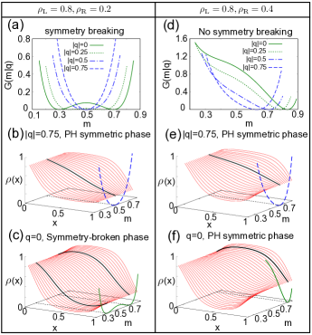
Figure 2: (a) Conditional LDF $G(m|q)=G(m,q)-G(q)$ for $\rho_{\text{L}}=0.8$, $\rho_{\text{R}}=0.2$ and $E=4$ as a function of $m$ and different values of $q$. (b) $\rho_{m,q}(x)$ for $|q|=0.75$ and different $m$’s, together with the associated $G(m|q)$. (c) Same results of panel (b) but for $q=0$. Two optimal profiles with high- and low-mass emerge (black solid lines). (d)-(f) Analogous results of panels (a)-(c) for $\rho_{\text{L}}=0.8$ and $\rho_{\text{R}}=0.4$.

DPT in the thermodynamics of currents.– When driven by $E\neq 0$ and/or $\rho_{\text{L}}\neq\rho_{\text{R}}$, the system relaxes to a nonequilibrium steady state characterized by an average current $\langle q\rangle$ and a non-trivial density profile $\rho_{\text{st}}(x)$ SM . Moreover, we can associate to any trajectory $\{\rho(x,t),j(x,t)\}_{0}^{\tau}$ an empirical current $q=\tau^{-1}\int_{0}^{\tau}dt\int_{0}^{1}dx~{}j(x,t)$. In the following we show how from the structure of the probability of this current, $P(q)$, we can predict the existence of DPTs associated with spontaneous symmetry breaking.

The probability $P(\{\rho,j\}_{0}^{\tau})$ of any trajectory can be computed from Eq. (1) via a path integral formalism Hurtado et al. (2014); Bertini et al. (2015); Derrida , and scales in the large-size limit as $P(\{\rho,j\}_{0}^{\tau})\sim\exp\{-L\,{\cal I}_{\tau}[\rho,j]\}$, with an action Bertini et al. (2015)

$${\cal I}_{\tau}[\rho,j]=\int_{0}^{\tau}dt\int_{0}^{1}dx\frac{\displaystyle\Big{(}j+D(\rho)\partial_{x}\rho-\sigma(\rho)E\Big{)}^{2}}{\displaystyle 2\sigma(\rho)}\,.$$ (2)

The probability $P(\{\rho,j\}_{0}^{\tau})$ represents the ensemble of space-time trajectories, from which one can obtain the statistics of any observable depending on $\{\rho,j\}_{0}^{\tau}$. In particular the probability of a given current $q$ can be obtained by minimizing the action functional (2) over all trajectories sustaining such current. This yields in the long-time limit $P(q)\sim\exp\{-\tau LG(q)\}$, with $G(q)=\lim_{\tau\rightarrow\infty}\frac{1}{\tau}\min^{*}_{\{\rho,j\}_{0}^{\tau}}{\cal I}_{\tau}(\rho,j)$ the current LDF, and ^∗ meaning that the minimization must be compatible with the prescribed constraints ($q,\rho_{\text{L,R}}$). The optimal trajectories $\rho_{q}(x,t)$ and $j_{q}(x,t)$ solution of this variational problem are then those adopted by the system in order to maintain the current $q$ over a long period of time, and turn out to be time-independent in many cases (a conjecture known as additivity principle Bodineau and Derrida (2004)).

Just as in standard critical phenomena, the action (2) contains the symmetries which are eventually broken. For WASEP with $\rho_{\text{R}}=1-\rho_{\text{L}}$ it is easy to check that the action (2) is invariant under the transformation $\rho\to 1-\rho$, $x\to 1-x$, referred to as PH symmetry (resulting from the symmetry of $\sigma(\rho)$ around $\rho=1/2$). The optimal density profile $\rho_{q}(x)$ typically inherits this PH symmetry, mapping onto itself under the above transformation. However, as detailed in the Supp. Mat. SM , for currents below a critical threshold ($|q|\leq|q_{c}|$) and large enough $E$, two different (but equally) optimal profiles $\rho_{q}^{\pm}(x)$ appear such that $\rho_{q}^{\pm}(x)\to 1-\rho_{q}^{\mp}(1-x)$, see inset to Fig. 1, giving rise to a second-order singularity in the current LDF. This spontaneous PH symmetry breaking can be easily understood Baek et al. (2017, 2018) by noting that, in order to sustain a low-current fluctuation, the system can react by either crowding with particles hence hindering motion, or rather emptying the lattice to minimize particle flow. Both tendencies break the action PH symmetry, eventually triggering the DPT.

Order parameter fluctuations.– To better understand this DPT, we study the joint fluctuations of the current and an appropriate global order parameter for the transition, much in the spirit of the paradigmatic Ising model of standard critical behavior Binney et al. (1992). A natural choice for this order parameter is the total mass in the system, which clearly characterizes the DPT in this case but also in more complex scenarios. Indeed, as shown in Fig. 1, the typical mass during a current fluctuation, $m_{q}\equiv\int_{0}^{1}dx\rho_{q}(x)$, exhibits a behavior strongly reminiscent of a standard $\mathbb{Z}_{2}$ phase transition, capturing the PH symmetry breaking. Defining the empirical mass for a trajectory as $m=\tau^{-1}\int_{0}^{\tau}dt\int_{0}^{1}dx\rho(x,t)$, the probability of observing a joint mass-current fluctuation for long times and large system sizes scales as $P(m,q)\sim\exp\{-\tau LG(m,q)\}$, with $G(m,q)=\lim_{\tau\rightarrow\infty}\frac{1}{\tau}\min^{*}_{\{\rho,j\}_{0}^{\tau}}{\cal I}_{\tau}(\rho,j)$ being the mass-current LDF, such that $G(q)=\min_{m}G(m,q)=G(m_{q},q)$. Within the additivity hypothesis Bodineau and Derrida (2004); Gorissen and Vanderzande (2012); Hurtado et al. (2014)

$$G(m,q)=\min_{\rho(x)}\int_{0}^{1}dx\frac{\displaystyle\Big{(}q+D(\rho)\partial_{x}\rho-\sigma(\rho)E\Big{)}^{2}}{\displaystyle 2\sigma(\rho)}\,,$$ (3)

with the optimal profile $\rho_{m,q}(x)$ subject to the constraint $m=\int_{0}^{1}dx\rho_{m,q}(x)$ as well as to fixed boundary conditions. The mass constraint can be implemented using a Lagrange multiplier, and we solve analitycally the resulting problem in terms of elliptic integrals and Jacobi elliptic functions, see SM . We note that the $\rho_{m,q}(x)$ so obtained can be classified attending to their extrema.

Fig. 2 illustrates our results for strong boundary gradients, well beyond the linear nonequilibrium regime. In particular, for PH-symmetric boundaries ($\rho_{\text{R}}=1-\rho_{\text{L}}$), the conditional mass-current LDF $G(m|q)\equiv G(m,q)-G(q)$ exhibits a peculiar change of behavior at a critical current $|q_{c}|$, see panel 2.a: while for $|q|>|q_{c}|$ the LDF $G(m|q)$ displays a single minimum at $m_{q}=1/2$, with an associated PH-symmetric optimal profile (Fig. 2.b), for $|q|<|q_{c}|$ two equivalent minima $m_{q}^{\pm}$ appear in $G(m|q)$, each one associated with a PH-symmetry-broken optimal profile $\rho_{q}^{\pm}(x)$, see Fig. 2.c, such that $\rho_{q}^{\pm}(x)\to 1-\rho_{q}^{\mp}(1-x)$. The emergence of this non-convex regime in $G(m|q)$ signals a $2^{\text{nd}}$-order DPT to a PH-symmetry-broken dynamical phase. On the other hand, for PH-asymmetric boundaries ($\rho_{\text{R}}\neq 1-\rho_{\text{L}}$), the governing action (2) is no longer PH-symmetric: the asymmetry favors one of the mass branches and the associated $G(m|q)$ displays a single global minimum $\forall q$ and an unique optimal profile (see Fig. 2.d-f), explaining why no DPT is observed in this case Gorissen and Vanderzande (2012). Still, $G(m|q)$ becomes non-convex for low enough currents, and for weak gradient asymmetry metastable-like local minima in $G(m|q)$ may appear SM .

Maxwell construction and additivity violation.– A natural question is whether time-dependent optimal trajectories exist which improve the additivity principle minimizers. The emergence of a non-convex regime in $G(m|q)$ for $|q|<|q_{c}|$ suggests a Maxwell-like instantonic solution in this region Bray and McKane (1989); Baek et al. (2018); Vroylandt and Verley (2018). In particular, as we show in SM , for PH-symmetric boundaries, fixed $|q|<|q_{c}|$ and $m\in(m_{q}^{-},m_{q}^{+})$, a trajectory which jumps smoothly (in a finite time) from $\rho_{q}^{-}(x)$ to $\rho_{q}^{+}(x)$ at time $t_{0}=\tau p$, with $p\equiv|m-m_{q}^{+}|/(m_{q}^{+}-m_{q}^{-})$, improves the additivity principle solution, yielding a straight Maxwell-like construction $G(m|q)=pG(m_{q}^{-}|q)+(1-p)G(m_{q}^{+}|q)$ for $m\in(m_{q}^{-},m_{q}^{+})$. This corresponds to a dynamical coexistence of the different symmetry-broken phases for $|q|<|q_{c}|$, as expected for a $1^{\text{st}}$-order DPT, see Fig. 1. Similar solutions exist for PH-asymmetric boundaries in regimes where $G(m|q)$ is non-convex, leading to metastable dynamical coexistence, and we note that the role of the instanton around $|q|\approx|q_{c}|$ can be affected by how the $L\to\infty$ and $\tau\to\infty$ limits are taken Baek et al. (2018).

Microscopic results: Spectral analysis.– Next we focus on the microscopic understanding of the symmetry-breaking DPT for current statistics. At the microscopic level, a configuration of the $1d$ WASEP is given by $C=\{n_{k}\}_{k=1,\ldots,L}$, where $n_{k}=0,1$ is the occupation number of the lattice’s $k^{\text{th}}$ site. Within the quantum Hamiltonian formalism for the master equation Schutz (2001), each configuration is represented as a vector in a Hilbert space, $\left|C\right\rangle=\bigotimes_{k=1}^{L}(n_{k},1-n_{k})^{T}$, with ^T denoting transposition. The complete information about the system is contained in a vector $\left|P\right\rangle=(P(C_{1}),P(C_{2}),...)^{T}=\sum_{i}P(C_{i})\left|C_{i}\right\rangle$, with $P(C_{i})$ representing the probabilities of the different configurations $C_{i}$. This probability vector evolves according to the master equation $\partial_{t}\left|P\right\rangle={\mathbb{W}}\left|P\right\rangle$, where ${\mathbb{W}}$ defines the Markov generator of the dynamics. Such generator can be tilted ${\mathbb{W}}^{\mu,\lambda}$ SM ; Touchette (2009); Hurtado et al. (2014) to bias the original stochastic dynamics in order to favor large (low) mass for $\mu<0$ ($\mu>0$) and large (low) currents for $\lambda>0$ ($\lambda<0$), with $\mu$ and $\lambda$ the conjugate parameters to the microscopic mass and current observables, respectively. The connection between the biased dynamics and the large deviation properties of our system is established through the largest eigenvalue of ${\mathbb{W}}^{\mu,\lambda}$ Touchette (2009); Garrahan (2018). Such eigenvalue, denoted by $\theta_{0}(\mu,\lambda)$, is nothing but the cumulant generating function of the observables $m$ and $q$, related to the LDF $G(m,q)$ via a Legendre transform, $\theta_{0}(\mu,\lambda)=L^{-1}\max_{m,q}[\lambda q-\mu Lm-G(m,q)]$.

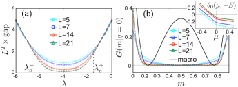
Figure 3: (a) Scaled spectral gap of the tilted generator as a function of $\lambda$ for $\mu=0$ and different system sizes. (b) Main panel: LDF $G(m|q=0)$ obtained by Legendre transforming $L\theta_{0}(\mu,\lambda=-E)$ together with macroscopic predictions. For increasing system sizes the microscopic $G(m|q=0)$ converges to the convex envelope of the macroscopic prediction. Inset: $\theta_{0}(\mu,-E)$ for different system sizes. Notice the kink at $\mu=0$. In all cases $\rho_{\text{L}}=\rho_{\text{R}}=0.5$ and $E=4$.

We now consider exact numerical diagonalization of ${\mathbb{W}}^{\mu,\lambda}$ for a particular case of PH-symmetric boundaries and no mass bias ($\mu=0$). Fig. 3.a shows that the diffusively-scaled spectral gap, $L^{2}[\theta_{0}(0,\lambda)-\theta_{1}(0,\lambda)]$, with $\theta_{1}(0,\lambda)$ the next-to-leading eigenvalue of ${\mathbb{W}}^{0,\lambda}$, tends to zero as $L$ increases in a region $\lambda_{c}^{-}<\lambda<\lambda_{c}^{+}$ (with $\lambda_{c}^{\pm}=-E\pm\sqrt{E^{2}-\pi^{2}}$) which corresponds to $|q|\leq|q_{c}|=\sqrt{E^{2}-\pi^{2}}/4$ as predicted SM ; Baek et al. (2017). This means that the $2^{\text{nd}}$-order DPT in current statistics unveiled above at the macroscopic level corresponds to an emerging degeneracy of the ground state of ${\mathbb{W}}^{\mu,\lambda}$ (i.e. that corresponding to the leading eigenvalue), in which the sub-leading eigenvalue coalesces with the leading one. Moreover, by varying $\mu$ for $\lambda=-E$ (equiv. $q=0$) a remarkable $1^{\text{st}}$-order-like behavior associated with a kink of $\theta_{0}(\mu,\lambda=-E)$ at $\mu=0$ is found, see inset to Fig. 3.b, consistent with the non-convex behavior of $G(m|q=0)$ found macroscopically and the associated dynamical coexistence of the two mass branches. Indeed, the numerical inverse Legendre transform of $\theta_{0}(\mu,\lambda=-E)$ converges to the convex envelope or Maxwell construction of the macroscopic prediction for $G(m|q=0)$, see Fig. 3.b.

The eigenspace associated to $\theta_{0}(\mu,\lambda)$ contains the microscopic information about the typical trajectories responsible for a given fluctuation (as parametrized by $\lambda$ and $\mu$). In this way, the emergence of a degeneracy as $L$ increases points out to the appearance of two competing (symmetry-broken) states. For large but finite $L$, the spectral gap is small but non-zero and the eigenspace of $\theta_{1}(\mu,\lambda)$ defines a long-lived metastable state Gaveau and Schulman (2006); a pedagogical review see J. Kurchan (2009); Macieszczak et al. (2016); Rose et al. (2016). Using Doob’s transform as a tool Chetrite and Touchette (2015a); Carollo et al. (2018b), one can show that any state in the degenerate (metastable) manifold is then given by a probability vector $\left|P_{\text{MS}}^{c}\right\rangle=\hat{L}_{0}(\left|R_{0}\right\rangle+c\left|R_{1}\right\rangle)$ SM . Here $\left|R_{i}\right\rangle$ ($\left|L_{i}\right\rangle$) is the right (left) eigenvector associated with $\theta_{i}(\mu,\lambda)$ ($i=0,1$), and $\hat{L}_{0}$ is a diagonal matrix whose elements $(\hat{L}_{0})_{ii}$ are the $i^{\text{th}}$ entries of $\left|L_{0}\right\rangle$. Moreover, $c\in[c_{1},c_{2}]$ is a constant with $c_{1}$ ($c_{2}$) the smallest (largest) entry of the vector $\left\langle L_{1}\right|\hat{L}_{0}^{-1}$. Interestingly, our microscopic approach shows that the high- and low-mass states in the symmetry-broken phase then correspond to the states $\left|P_{\text{MS}}^{c_{1},c_{2}}\right\rangle$, from which the average density profile in each phase can be computed. Fig. 4 shows the profiles so obtained from the exact numerical diagonalization of ${\mathbb{W}}^{\mu,\lambda}$ for two different gradients, and the convergence to the macroscopic prediction as $L$ increases is clear.

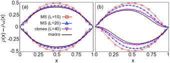
Figure 4: (a) Optimal density profiles for the open WASEP with $\rho_{\text{L}}=\rho_{\text{R}}=0.5$ and $E=4$ conditioned to have a current $q=0$. Macroscopic predictions (black solid lines) and simulation results using the cloning algorithm for $L=40$ (purple down triangles). Profiles associated with the extremal metastable states for $L=10$ (red squares) and $L=20$ (blue up triangles). (b) Same results for $\rho_{\text{L}}=0.8$ and $\rho_{\text{R}}=0.2$.

Direct observation of the DPT.– So far, we have obtained clear indications of a symmetry-breaking DPT both from a macroscopic approach and a microscopic (spectral) analysis. The question remains as to whether this phenomenon is observable in simulations, which allow to reach larger system sizes. To address this we have performed extensive rare event simulations using the cloning Monte Carlo method Giardinà et al. (2006); Lecomte and Tailleur ; Tailleur and Lecomte (2009); Giardinà et al. (2011) to study current statistics in the open $1d$ WASEP. Starting from random initial configurations, we have measured the optimal density profiles adopted by the system to sustain a highly atypical current, namely $q=0$, using a population of $10^{4}$ clones and $L=40$. To capture the possible symmetry breaking, we average separately profiles with a total mass above and below $1/2$. Fig. 4.a shows the result for $\rho_{\text{L}}=\rho_{\text{R}}=0.5$, while Fig. 4.b displays data for $\rho_{\text{L}}=0.8$ and $\rho_{\text{R}}=0.2$ (in both cases $E=4$). The measured high- and low-mass optimal profiles again converge towards the macroscopic predictions, strongly supporting our results on the PH-symmetry-breaking scenario.

Conclusions.– We have analyzed from a hydrodynamic, microscopic and computational point of view a $2^{\text{nd}}$-order DPT in the current statistis of a paradigmatic driven diffusive system, the open $1d$ WASEP, unveiling the full dynamical phase diagram for arbitrary current fluctuations and boundary driving. For that we have investigated the joint fluctuations of the current and a collective order parameter, the total mass in the system, finding that the associated LDF becomes non-convex for low enough currents. Microscopically, we link the observed DPT with an emerging degeneracy of the ground state of the tilted dynamical generator, from which the macroscopic optimal profiles can be computed. Our predictions are confirmed by the observation of this DPT phenomenon for the first time in rare event simulations.

We thank Vivien Lecomte for insightful discussions. The research leading to these results has received funding from the EPSRC Grant No. EP/M014266/1 and the Spanish Ministry MINECO project FIS2017-84256-P. C.P.E. acknowledges the funding received from the European Union’s Horizon 2020 research and innovation programme under the Marie Sklodowska-Curie Cofund Programme Athenea3I Grant Agreement No. 754446. C.P.E, P.I.H and J.P.G acknowledge as well the hospitality and support of the International Centre for Theoretical Sciences (ICTS) in Bangalore (India), where part of this work was developed during the program Large deviation theory in statistical physics: Recent advances and future challenges (Code: ICTS/Prog-ldt/2017/8). We are also grateful for access to the University of Nottingham High Performance Computing Facility, and for the computational resources and assistance provided by PROTEUS, the super-computing center of iC1 in Granada, Spain.

SUPPLEMENTAL MATERIAL

Carlos Pérez-Espigares,^1,2 Federico Carollo,¹ Juan P. Garrahan,¹ and Pablo I. Hurtado²

¹School of Physics and Astronomy, and Centre for the Mathematics and Theoretical Physics of Quantum Non-Equilibrium Systems, University of Nottingham, Nottingham, NG7 2RD, United Kingdom
²Departamento de Electromagnetismo y Física de la Materia, and Institute Carlos I for Theoretical and Computational Physics, Universidad de Granada, Granada 18071, Spain

In this Supplemental Material we solve the macroscopic fluctuation theory (MFT) equations for the joint current and mass fluctuations of the one-dimensional ($1d$) weakly asymmetric simple exclusion process (WASEP) coupled to boundary particle reservoirs at arbitrary densities or chemical potentials. This model belongs in a large class of driven diffusive systems of theoretical and technological interest. MFT Bertini et al. (2015) provides a detailed description of dynamical fluctuations in general driven diffusive systems, starting from the hydrodynamic evolution equation for the system of interest and the sole knowledge of two transport coefficients, which can be measured experimentally. In particular, MFT offers explicit predictions for the large-deviation functions (LDFs) which characterize the fluctuations of different observables, as well as the associated trajectories in phase space responsible of these fluctuations.

After a brief but self-consistent presentation of MFT in §S1 and a characterization of the nonequilibrium steady state of the $1d$ open WASEP under arbitrary driving (see §S2), we proceed to solve analytically in §S3 the MFT equations for the joint mass-current statistics of this model, understanding along the way the symmetry-breaking dynamical phase transition described in the main text. Key to this calculation is the additivity conjecture Bodineau and Derrida (2004), which assumes that the optimal trajectories responsible of a trajectory are time-independent. We explore in §S4 the possibility of additivity violations in the form of time-dependent, instantonic solutions to the MFT equations in regimes where the joint current-mass LDF becomes non-convex. Finally, we study in §S5 from a microscopic point of view the DPT found at the macroscopic level, using in particular the quantum Hamiltonian formalism for the master equation and the tilted dynamical generator.

S1 A crash course on MFT

We hence consider systems described at the mesoscopic level by a continuity equation of the form

$$\partial_{t}\rho+\partial_{x}j=0\,,$$ (S1)

where $\rho(x,t)$ and $j(x,t)$ are the density and current fields, respectively, and $x\in[0,1]$ and $t$ are the macroscopic space and time variables, obtained after a diffusive scaling limit such that $x=\tilde{x}/L$ and $t=\tilde{t}/L^{2}$, with $\tilde{x}$ and $\tilde{t}$ the equivalent microscopic variables and $L$ the system size in natural units. The system is coupled at the boundaries to particle reservoirs at densities $\rho_{\text{L,R}}$, so the boundary conditions for the density field are $\rho(0,t)=\rho_{\text{L}}$ and $\rho(1,t)=\rho_{\text{R}}$ $\forall t$. The current field in eq. (S1) is in general a fluctuating quantity, and can be written as

$$j(x,t)=-D(\rho)\partial_{x}\rho(x,t)+\sigma(\rho)E+\xi(x,t).$$ (S2)

The first two terms in the rhs are just Fick’s law, which express the proportionality of the current to the density gradient and the external field $E$, with $D(\rho)$ and $\sigma(\rho)$ the diffusivity and mobility transport coefficients (which might be nonlinear functions of the local density). The last term $\xi(x,t)$ is a weak Gaussian white noise, such that

$$\langle\xi(x,t)\rangle=0,\qquad\langle\xi(x,t)\xi(x^{\prime},t^{\prime})\rangle=\frac{\sigma(\rho)}{L}\delta(x-x^{\prime})\delta(t-t^{\prime})\,.$$ (S3)

This noise term accounts for all fast degrees of freedom which are integrated out in the coarse-graining proceduce which results in the mesoscopic hydrodynamic description (S1)-(S2). After some relaxation time, a system described by the above set of equations reaches a nonequilibrium steady state characterized by a (typically inhomogeneous) density profile $\rho_{\text{st}}(x)$ compatible with the above boundary conditions, and a nonzero average current $\langle q\rangle=-D(\rho_{\text{st}})\partial_{x}\rho_{\text{st}}+\sigma(\rho_{\text{st}})E$ constant across space. Note that, for WASEP, the two key transport coefficients are $D(\rho)=\frac{1}{2}$ and $\sigma(\rho)=\rho(1-\rho)$ Derrida (1998); Chou et al. (2011), and Section §S2 below describes the steady-state solution of the above hydrodynamic equations for the $1d$ open WASEP.

A simple path integral calculation starting from Eqs. (S1)-(S2) then shows that the probability of a given field trajectory $\{\rho,j\}_{0}^{\tau}$ obeys a large deviation principle of the form $P(\{\rho,j\}_{0}^{\tau})\sim\exp(-L{\cal I}_{\tau}[\rho,j])$, with an action given by Bertini et al. (2015); Derrida ; Hurtado et al. (2014)

$${\cal I}_{\tau}[\rho,j]=\int_{0}^{\tau}dt\int_{0}^{1}dx\frac{[j+D(\rho)\partial_{x}\rho-E\sigma(\rho)]^{2}}{2\sigma(\rho)}\,,$$ (S4)

with $\rho(x,t)$ and $j(x,t)$ coupled via the continuity equation $\partial_{t}\rho+\partial_{x}j=0$ (in any other case ${\cal I}_{\tau}[\rho,j]\to\infty$). We are interested here in the joint statistics for fluctuations of the spacetime-integrated current $q$ and mass $m$. These two empirical observables are defined as

$$q = \frac{1}{\tau}\int_{0}^{\tau}dt\int_{0}^{1}dx\,j(x,t)\,,$$ (S5)

$$m = \frac{1}{\tau}\int_{0}^{\tau}dt\int_{0}^{1}dx\,\rho(x,t)\,.$$ (S6)

The probability of observing a given $q$ and $m$ can now be written as a path integral over all possible trajectories $\{\rho,j\}_{0}^{\tau}$, weighted by its probability measure $P(\{j,\rho\}_{0}^{\tau})$, and restricted to those trajectories compatible with the values of $q$ and $m$ in Eqs. (S5) and (S6), respectively, the continuity equation (S1) at every point of space and time, and the fixed boundary conditions for the density field. For long times and large system sizes, this sum over trajectories is dominated by the associated saddle point and scales as $P(m,q)\sim\exp\{-\tau LG(m,q)\}$, where $G(m,q)$ is the mass-current large deviation function (LDF) given by

$$G(m,q)=\lim_{\tau\rightarrow\infty}\frac{1}{\tau}\min_{\{\rho,j\}_{0}^{\tau}}{\cal I}_{\tau}(\rho,j)\,.$$ (S7)

The density and current fields solution of this variational problem, denoted here as $\rho_{m,q}(x,t)$ and $j_{m,q}(x,t)$, can be interpreted as the optimal trajectory the system follows in order to sustain a long-time mass and current joint fluctuation, and are in general time-dependent.

However, in most applications of MFT to study fluctuations of time-integrated observables in open systems, such as (S5)-(S6), it has been found that the optimal trajectory $\{\rho_{m,q},j_{m,q}\}_{0}^{\tau}$ is indeed time-independent. Physically this means that, in order sustain a given mass-current long-time fluctuation, the system of interest settles after a negligible initial transient into a time-independent state (possibly followed by an equally negligible final transient). This property, known as Additivity Principle in literature Bodineau and Derrida (2004); Bertini et al. (2005, 2006); Hurtado and Garrido (2009b, 2011); Saito and Dhar (2011); Hurtado et al. (2011); Pérez-Espigares et al. (2013); Hurtado et al. (2013); Žnidarič (2014); Bertini et al. (2015); Shpielberg and Akkermans (2016); Pérez-Espigares et al. (2016); Tizón-Escamilla et al. (2017, 2017), strongly simplifies the variational problem at hand. In particular, the mass-current LDF now reads

$$G(m,q)=\min_{\rho(x)}\int_{0}^{1}dx\frac{\displaystyle\left[q+D(\rho)\rho^{\prime}(x)-\sigma(\rho)E\right]^{2}}{\displaystyle 2\sigma(\rho)}\,.$$ (S8)

The optimal density profile solution of this simpler variational problem, $\rho_{m,q}(x)$, is subject to to the additional constraint

$$m=\int_{0}^{1}\rho_{m,q}(x)\,dx\,,$$ (S9)

and the optimal current field is simply $j_{m,q}(x)=q$ due to the continuity equation (S1) and the time-independence of the dominant trajectory. The integral constraint (S9) can be implemented using a Lagrange multiplier $\lambda$ which will be fixed a posteriori to enforce the constraint. We hence define a new function

$$G(\lambda,q)=\min_{\rho(x)}\int_{0}^{1}dx\left\{\frac{\displaystyle\left[q+D(\rho)\rho^{\prime}(x)-\sigma(\rho)E\right]^{2}}{\displaystyle 2\sigma(\rho)}-\lambda\rho(x)\right\}\,.$$ (S10)

The optimal density field for this variational problem is the solution of the following Euler-Lagrange equation

$$q^{2}\left(\frac{1}{2\sigma(\rho)}\right)^{\prime}+\frac{E^{2}}{2}\sigma^{\prime}(\rho)-\rho^{\prime\prime}(x)\frac{D(\rho)^{2}}{\sigma(\rho)}-\rho^{\prime}(x)^{2}\left(\frac{D(\rho)^{2}}{2\sigma(\rho)}\right)^{\prime}=\lambda,$$ (S11)

where the ^′ means derivative with respect to the argument, e.g. $\sigma^{\prime}(\rho)=\frac{d\sigma(\rho)}{d\rho}$ and $\rho^{\prime}(x)=\frac{d\rho(x)}{dx}$. Multiplying both sides of this equation by $\rho^{\prime}(x)$, we arrive easily to

$$\frac{d}{dx}\left[\frac{q^{2}}{2\sigma(\rho)}-\lambda\rho(x)+\frac{E^{2}}{2}\sigma(\rho)-\rho^{\prime}(x)^{2}\frac{D(\rho)^{2}}{2\sigma(\rho)}\right]=0\,,$$ (S12)

which can be trivially integrated once to yield

$$D(\rho)^{2}\left(\frac{d\rho(x)}{dx}\right)^{2}=q^{2}+2\left(K-\lambda\rho\right)\sigma(\rho)+E^{2}\sigma(\rho)^{2}\,,$$ (S13)

where $K$ is an integration constant which allows us to fix the correct boundary condition at one of the two ends, $\rho_{\lambda,q}(0)=\rho_{\text{L}}$ and $\rho_{\lambda,q}(1)=\rho_{\text{R}}$ (the other boundary value is given to solve the previous first-order differential equation). Interestingly, the optimal density field solution of this differential equation does not depend on the sign of the current $q$ or the external field $E$, as they both appear squared in Eq. (S13). This fact is ultimately a macroscopic manifestation of the time-reversibility of microscopic dynamics. The value of the Lagrange multiplier $\lambda=\lambda(m,q)$ can be now fixed by imposing that the total mass associated to the solution $\rho_{\lambda,q}(x)$ of the above differential equation is just $m$, i.e.

$$m=\int_{0}^{1}\rho_{\lambda,q}(x)\,dx\,.$$ (S14)

Our aim in the following sections is to solve this variational problem for the $1d$ open WASEP, for which the key transport coefficients are $D(\rho)=1/2$ and $\sigma(\rho)=\rho(1-\rho)$. However, before proceeding with the analysis of fluctuations, we focus briefly on the steady state behavior.

S2 Steady state for the $1d$ open WASEP

In this section we derive the steady state current $\langle q\rangle$ and density profile $\rho_{\text{st}}(x)$ for the $1d$ open WASEP driven by an arbitrary external density gradient and possibly by an additional external field $E$. These steady state properties are given by Fick’s law, which for $D(\rho)=1/2$ and $\sigma(\rho)=\rho(1-\rho)$ simply reads

$$\langle q\rangle=-\frac{1}{2}\frac{d\rho_{\text{st}}(x)}{dx}+E\rho_{\text{st}}(x)[1-\rho_{\text{st}}(x)]\,,$$ (S15)

with boundary conditions $\rho_{\text{st}}(0)=\rho_{\text{L}}$ and $\rho_{\text{st}}(1)=\rho_{\text{R}}$. The previous equation can be easily solved

$$x=\int_{\rho_{\text{L}}}^{\rho_{\text{st}}(x)}\frac{d\rho}{2[E\rho(1-\rho)-\langle q\rangle]}=-\frac{1}{\theta}\tan^{-1}\left(\frac{E}{\theta}(2\rho-1)\right)\Bigg{|}_{\rho_{\text{L}}}^{\rho_{\text{st}}(x)}\equiv-\frac{1}{\theta}{\cal T}_{\theta}(\rho)\Bigg{|}_{\rho_{\text{L}}}^{\rho_{\text{st}}(x)}\,,$$

with the definitions $\theta\equiv\sqrt{E(4\langle q\rangle-E)}$ and ${\cal T}_{\theta}(\rho)\equiv\tan^{-1}\left(\frac{E}{\theta}(2\rho-1)\right)$. Equivalently

$$x=\frac{1}{\theta}\left[{\cal T}_{\theta}(\rho_{\text{L}})-{\cal T}_{\theta}(\rho_{\text{st}}(x))\right]\,.$$

By imposing now that $\rho_{\text{st}}(1)=\rho_{\text{R}}$, we obtain an implicit equation for the constant $\theta$, i.e.

$$\theta={\cal T}_{\theta}(\rho_{\text{L}})-{\cal T}_{\theta}(\rho_{\text{R}})\,.$$

This equation for $\theta(\rho_{\text{L}},\rho_{\text{R}},E)$ cannot be solved analytically in general. However, it might be solved numerically for every external parameter 3-tuple $(\rho_{\text{L}},\rho_{\text{R}},E)$. From this solution one can obtain the steady-state current

$$\langle q\rangle=\frac{1}{4}\left(E+\frac{\theta^{2}}{E}\right)$$ (S16)

and the stationary density profile

$$\rho_{\text{st}}(x)=\frac{1}{2}\left\{1+\frac{\theta}{E}\tan\left[{\cal T}_{\theta}(\rho_{\text{L}})-\theta x\right]\right\}\,.$$ (S17)

Fig. S5 shows steady-state profiles and stationary currents for different values of $(\rho_{\text{L}},\rho_{\text{R}},E)$.

Figure S5: (a) Steady-state density profile $\rho_{\text{st}}(x)$ for the $1d$ open WASEP for a symmetric gradient with boundary densities $\rho_{\text{L}}=0.8$ and $\rho_{\text{R}}=0.2$, and external fields $E\in[1,50]$ increasing as $E_{k}=50^{k/10}$ with $k\in[0,10]$. (b) Same results as in (a), but for an asymmetric gradient with boundary densities $\rho_{\text{L}}=0.6$ and $\rho_{\text{R}}=0.45$. (c) Steady state current $\langle q\rangle$ vs $\rho_{\text{L}}$ for external field $E=4$ and two right boundary densities, namely $\rho_{\text{R}}=0.2$ and $\rho_{\text{R}}=0.45$.

S3 Joint mass-current fluctuations in the $1d$ open WASEP

We now return to our original problem of determining the optimal density field associated to a mass-current fluctuation in the $1d$ open WASEP. The governing differential equation (S13) reads in this case

$$\frac{1}{4}\left(\frac{d\rho}{dx}\right)^{2}=q^{2}+2(K-\lambda\rho)\rho(1-\rho)+E^{2}\rho^{2}(1-\rho)^{2}\,,$$ (S18)

with boundary conditions $\rho(0)=\rho_{\text{L}}$ and $\rho(1)=\rho_{\text{R}}$. Without loss of generality, we assume from now on that $\rho_{\text{L}}\geq\rho_{\text{R}}$ and $E>0$; equivalent results to those described below hold in other situations. Note also that the case $E=0$ results in a simpler problem lacking any dynamical phase transition Baek et al. (2017), so it won’t be studied here. The rhs of Eq. (S18) defines a fourth-order polynomial in $\rho$,

$$\pi_{0}(\rho)\equiv q^{2}+2(K-\lambda\rho)\rho(1-\rho)+E^{2}\rho^{2}(1-\rho)^{2}\equiv E^{2}\pi(\rho)\,,$$ (S19)

whose roots will play a key role in the analysis of possible solutions. In particular, the real roots of $\pi(\rho)$ (equivalently $\pi_{0}(\rho)$) define the possible extrema of the optimal density field, though as we discuss next not all real roots correspond necessarily to extrema of the profile.

A first observation is that, for $\rho_{\text{L}}>\rho_{\text{R}}$, no (local) extrema of the optimal profile $\rho_{\lambda,q}(x)$ can lie within the $\rho$-interval $(\rho_{\text{R}},\rho_{\text{L}})$. To see why, let’s assume for a moment that there exists a local extremum $\rho_{a}\in(\rho_{\text{R}},\rho_{\text{L}})$, i.e. a real root $\rho_{a}\in\mathbb{R}$ such that $\pi(\rho_{a})=0$ and $\pi^{\prime}(\rho_{a})\neq 0$. If $\rho_{a}=\rho(x_{a})$ is a local maximum, it must be reached from below from both sides (as $x\to x_{a}^{\pm}$), and this is not possible since $\rho_{\text{L}}>\rho_{a}$. Equivalently, if $\rho_{a}$ is a local minimum it should be reached from above from both sides, and this is again not possible because $\rho_{\text{R}}<\rho_{a}$. Hence no local extrema of the density profile can lie in the interval $(\rho_{\text{R}},\rho_{\text{L}})$. Similarly, only one maximum can exists above $\rho_{\text{L}}$. Indeed, if two maxima $\rho_{a}>\rho_{b}>\rho_{\text{L}}$ exist (one local, the other global), they must be separated by a local minimum $\rho_{c}>\rho_{\text{L}}$. By definition, this local minimum must be reached from above from both sides, and this is again impossible since $\rho_{\text{L}}<\rho_{c}$. An equivalent argument shows that only one minimum can exists below $\rho_{\text{R}}$. Moreover, a numerical analysis of the differential equation (S18) shows that no inflection points, for which $\pi(\rho)=0=\pi^{\prime}(\rho)$ simultaneously, are to be expected in the solutions, so we can safely assume that only maxima and minima are possible. These arguments therefore suggest that the optimal density profile solution of the Eq. (S18) can be either (a) monotonous, or contain (b) a single maximum, (c) a single minimum, or at most (d) one maximum and one minimum.

Before embarking on the general solution of the differential equation (S18), let us summarize the global solution strategy. As we will show below, the resulting density profile can be written as a rational function of Jacobi elliptic functions (either sn, cn or tn Jacobi functions Byrd and Friedman (1971), depending on the root structure of the polynomial $\pi(\rho)$ defined above). This density profile will be a parametric function of the current $q$ and the external field $E$, as well as the constants $K$ and $\lambda$, i.e. $\rho(x)=\rho(x;q,E,K,\lambda)$. These two latter constants must be fixed by imposing simultaneously the correct right boundary density $\rho_{\text{R}}$ and the total mass $m$, i.e.

$$\rho(x=1;q,E,K,\lambda)=\rho_{\text{R}}\,,\qquad\qquad\int_{0}^{1}\rho(x;q,E,K,\lambda)\,dx=m\,.$$ (S20)

Although we find below explicit solutions for $\rho(x;q,E,K,\lambda)$, the simultaneous solution of the previous equations requires numerical methods to determine the values of $K$ and $\lambda$ associated to a joint fluctuation of the current $q$ and mass $m$ under external field $E$. Moreover, the lack of intuition about the possible values of the constants $K$ and $\lambda$ for a given set of parameters $(m,q,E)$ calls for an alternative codification of these two constants in terms of more physical quantities. In particular, defining $\rho^{\prime}_{\text{L,R}}(m,q,E)\equiv\rho^{\prime}(x=0,1)$ as the slope of the optimal density profile at the left (L) and right (R) boundary, respectively, which depend on the external parameters $(m,q,E)$, we can see from Eq. (S18) that

$$\frac{1}{4}(\rho^{\prime}_{\text{L,R}})^{2}=q^{2}+2(K-\lambda\rho_{\text{L,R}})\rho_{\text{L,R}}(1-\rho_{\text{L,R}})+E^{2}\rho_{\text{L,R}}^{2}(1-\rho_{\text{L,R}})^{2}\,,$$ (S21)

which allows to write the constants $K$ and $\lambda$ in terms of the more intuitive boundary slopes $\rho^{\prime}_{\text{L,R}}(m,q,E)$, i.e.

$$K(m,q,E)=\frac{\Lambda_{\text{R}}(m,q,E)\rho_{\text{L}}-\Lambda_{\text{L}}(m,q,E)\rho_{\text{R}}}{\rho_{\text{L}}-\rho_{\text{R}}}\,,\qquad\lambda(m,q,E)=\frac{\Lambda_{\text{R}}(m,q,E)-\Lambda_{\text{L}}(m,q,E)}{\rho_{\text{L}}-\rho_{\text{R}}}\,,$$ (S22)

where we have defined

$$\Lambda_{\text{L,R}}(m,q,E)\equiv\frac{\frac{1}{4}(\rho^{\prime}_{\text{L,R}})^{2}(m,q,E)-q^{2}-E^{2}\rho_{\text{L,R}}^{2}(1-\rho_{\text{L,R}})^{2}}{2\rho_{\text{L,R}}(1-\rho_{\text{L,R}})}\,.$$ (S23)

Hence, for a given external field $E$ and fixed values of the current $q$ and the mass $m$, one has to find numerically the slopes $\rho^{\prime}_{\text{L,R}}(m,q,E)$ such that

$$\rho(x=1;q,E,\rho^{\prime}_{\text{L}},\rho^{\prime}_{\text{R}})=\rho_{\text{R}}\,,\qquad\qquad\int_{0}^{1}\rho(x;q,\rho^{\prime}_{\text{L}},\rho^{\prime}_{\text{R}})\,dx=m\,,$$ (S24)

where $\rho(x;q,E,\rho^{\prime}_{\text{L}},\rho^{\prime}_{\text{R}})$ is the optimal profile solution of our variational problem. Recalling now that $\rho_{\text{L}}\geq\rho_{\text{R}}$, it is interesting to note that fixing the sign of the boundary slopes $\rho^{\prime}_{\text{L,R}}(m,q,E)$ determines whether the resulting profiles is either monotonous ($\rho^{\prime}_{\text{L}}<0,\rho^{\prime}_{\text{R}}<0$) or exhibits a single maximum ($\rho^{\prime}_{\text{L}}>0,\rho^{\prime}_{\text{R}}<0$), a single minimum ($\rho^{\prime}_{\text{L}}<0,\rho^{\prime}_{\text{R}}>0$), or one maximum and one minimum ($\rho^{\prime}_{\text{L}}>0,\rho^{\prime}_{\text{R}}>0$; we discuss below the reason why the maximum comes before the minimum).

We turn now to the explicit solution of the ordinary differential equation (S18), which can be written as $\rho^{\prime}(x)=\pm 2|E|\sqrt{\pi(\rho)}$, where the sign depends on the section of the profile analyzed. Since $\rho_{\text{L}}\geq\rho_{\text{R}}$, monotonous profiles have $\rho^{\prime}(x)\leq 0$ $\forall x\in[0,1]$, and the differential equation can be integrated to yield

$$2|E|x=\int_{\rho(x)}^{\rho_{\text{L}}}\frac{d\rho}{\sqrt{\pi(\rho)}}\qquad\qquad\text{(monotonous profile)}.$$ (S25)

For optimal profiles containing a single maximum $\rho_{+}=\rho(x_{+})$, such that $\pi(\rho_{+})=0$, we have $\rho^{\prime}(x)=+2|E|\sqrt{\pi(\rho)}$ $\forall x\in[0,x_{+}]$ and $\rho^{\prime}(x)=-2|E|\sqrt{\pi(\rho)}$ $\forall x\in[x_{+},1]$, and hence

$$2|E|x=\left\{\begin{array}[]{l l}\displaystyle\int_{\rho_{\text{L}}}^{\rho(x)}\frac{d\rho}{\sqrt{\pi(\rho)}}&\quad 0\leq x\leq x_{+}\\ \phantom{aaa}\\ \displaystyle 2|E|x_{+}+\int_{\rho(x)}^{\rho_{+}}\frac{d\rho}{\sqrt{\pi(\rho)}}&\quad x_{+}<x\leq 1\end{array}\right.\qquad\qquad\text{(single-maximum profile)},$$ (S26)

where $\displaystyle 2|E|x_{+}=\int_{\rho_{\text{L}}}^{\rho_{+}}\frac{d\rho}{\sqrt{\pi(\rho)}}$ defines the position of the maximum. Next, for optimal profiles containing a single minimum $\rho_{-}=\rho(x_{-})$, such that $\pi(\rho_{-})=0$, one can show equivalently

$$2|E|x=\left\{\begin{array}[]{l l}\displaystyle\int_{\rho(x)}^{\rho_{\text{L}}}\frac{d\rho}{\sqrt{\pi(\rho)}}&\quad 0\leq x\leq x_{-}\\ \phantom{aaa}\\ \displaystyle 2|E|x_{-}+\int_{\rho_{-}}^{\rho(x)}\frac{d\rho}{\sqrt{\pi(\rho)}}&\quad x_{-}<x\leq 1\end{array}\right.\qquad\qquad\text{(single-minimum profile)},$$ (S27)

where now $\displaystyle 2|E|x_{-}=\int_{\rho_{-}}^{\rho_{\text{L}}}\frac{d\rho}{\sqrt{\pi(\rho)}}$ locates the minimum. Finally, for profiles with a maximum $\rho_{+}=\rho(x_{+})$ and a minimum $\rho_{-}=\rho(x_{-})$, with $\pi(\rho_{+})=0=\pi(\rho-)$, it is easy to see that

$$2|E|x=\left\{\begin{array}[]{l l}\displaystyle\int_{\rho_{\text{L}}}^{\rho(x)}\frac{d\rho}{\sqrt{\pi(\rho)}}&\quad 0\leq x\leq x_{+}\,,\\ \phantom{aaa}\\ \displaystyle 2|E|x_{+}+\int_{\rho(x)}^{\rho_{+}}\frac{d\rho}{\sqrt{\pi(\rho)}}&\quad x_{+}<x\leq x_{-}\,,\\ \phantom{aaa}\\ \displaystyle 2|E|x_{-}+\int_{\rho_{-}}^{\rho(x)}\frac{d\rho}{\sqrt{\pi(\rho)}}&\quad x_{-}<x\leq 1\,.\end{array}\right.\qquad\qquad\text{(max-min profile)},$$ (S28)

with

$$2|E|x_{+} = \displaystyle\int_{\rho_{\text{L}}}^{\rho_{+}}\frac{d\rho}{\sqrt{\pi(\rho)}}\,,$$ (S29)

$$2|E|x_{-} = \displaystyle 2|E|x_{+}+\int_{\rho_{-}}^{\rho_{+}}\frac{d\rho}{\sqrt{\pi(\rho)}}\,.$$ (S30)

Here we implicitly assume that $x_{+}<x_{-}$, i.e. the maximum comes before the minimum. This is a consequence of the choice $\rho_{\text{L}}\geq\rho_{\text{R}}$, which makes the cost of reversing the extrema non-optimal from a variational point of view, see Eq. (S8).

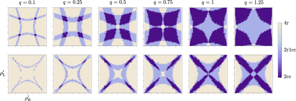
Figure S6: Density plot of the structure of zeroes of the polynomial $\pi(\rho)$ as a function of the boundary slopes $\rho^{\prime}_{\text{L,R}}(m,q,E)\in[-3,3]$ for external field $E=4$ and varying values of the current $q\in[0,1.25]$. Results for two density gradients are shown, namely $(\rho_{\text{L}}=0.8,\rho_{\text{R}}=0.2)$ (symmetric gradient, top row) and $(\rho_{\text{L}}=0.6,\rho_{\text{R}}=0.45)$ (asymmetric gradient, bottom row).

In all cases, the integrals appearing in Eqs. (S25)-(S28) are elliptic integrals of the first kind, whose inverse solution can be written in terms of Jacobi elliptic functions Byrd and Friedman (1971), depending on the structure of zeroes of the 4${}^{\text{th}}$-order polynomial $\pi(\rho)$. Since this polynomial is always real, its 4 roots can be either two pairs of complex conjugate numbers ($\rho_{1},\rho_{1}^{*},\rho_{2},\rho_{2}^{*}\in\mathbb{C}$, denoted as case 2cc), two real roots accompanied by a single pair of complex conjugate roots ($\rho_{1},\rho_{2}\in\mathbb{R},~{}\rho_{3},\rho_{3}^{*}\in\mathbb{C}$, denoted as case 2r1cc), or 4 different real roots ($\rho_{1},\rho_{2},\rho_{3},\rho_{4}\in\mathbb{R}$, denoted as case 4r). Note that all possible combinations do appear in the solution of this variational problem. As an example, Fig. S6 shows density plots for the structure of zeroes of the polynomial $\pi(\rho)$ for a fixed external field $E=4$ (used below) as a function of the possible boundary slopes of the optimal density field, $\rho^{\prime}_{\text{L,R}}(m,q,E)$, for two different density gradients. We now study each of the cases separately.

S3.1 Two pairs of complex conjugate roots

In this case, due to the absence of real roots, the optimal density profile must be monotonous. This behavior will be dominant for small mass and current fluctuations, i.e. close to the average behavior. If we denote the complex roots as $\rho_{1},\rho_{1}^{*},\rho_{2},\rho_{2}^{*}\in\mathbb{C}$, the polynomial can be written as $\pi(\rho)=(\rho-\rho_{1})(\rho-\rho_{1}^{*})(\rho-\rho_{2})(\rho-\rho_{2}^{*})$. Defining now $b_{i}\equiv\text{Re}(\rho_{i})$ and $a_{i}\equiv|\text{Im}(\rho_{i})|$, with $i=1,2$, and introducing the constants $A^{2}\equiv(b_{1}-b_{2})^{2}+(a_{1}+a_{2})^{2}$, $B^{2}\equiv(b_{1}-b_{2})^{2}+(a_{1}-a_{2})^{2}$ and $y_{1}\equiv b_{1}-a_{1}g_{1}$, with

$$g_{1}^{2}\equiv\frac{4a_{1}^{2}-(A-B)^{2}}{(A+B)^{2}-4a_{1}^{2}}\,,$$ (S31)

we can solve Byrd and Friedman (1971) the integral (S25)

$$2|E|x=\int_{y_{1}}^{\rho_{\text{L}}}\frac{d\rho}{\sqrt{\pi(\rho)}}-\int_{y_{1}}^{\rho(x)}\frac{d\rho}{\sqrt{\pi(\rho)}}=\frac{2}{A+B}\left[F\left(\varphi(\rho_{\text{L}}),\frac{4AB}{(A+B)^{2}}\right)-F\left(\varphi(\rho(x)),\frac{4AB}{(A+B)^{2}}\right)\right]\,,$$ (S32)

with

$$\varphi(z)\equiv\tan^{-1}\left(\frac{z-b_{1}+a_{1}g_{1}}{a_{1}+g_{1}b_{1}-g_{1}z}\right)\,,$$ (S33)

and where $F(\varphi(z),k^{2})$ is the incomplete elliptic integral of the first kind of amplitude $\varphi(z)$ and modulus $k^{2}$ Byrd and Friedman (1971). As originally shown by Abel and Jacobi, this elliptic integral can be inverted Byrd and Friedman (1971). Indeed, if $u\equiv F(\varphi(z),k^{2})$, then $\tan\varphi(z)=\text{tn}(u,k^{2})$, where $\text{tn}(u,k^{2})$ is the Jacobi tn elliptic function Byrd and Friedman (1971). Applying this inversion formula to

$$F\Big{(}\varphi(\rho(x)),\kappa_{\varphi}^{2}\Big{)}=F_{\varphi}^{L}-(A+B)|E|x\,,$$ (S34)

where we have defined for simplicity $\kappa_{\varphi}^{2}\equiv 4AB/(A+B)^{2}$ and $F_{\varphi}^{L}\equiv F\left(\varphi(\rho_{\text{L}}),\kappa_{\varphi}^{2}\right)$, and solving for $\rho(x)$ we find for the case of two complex conjugate roots (2cc)

$$\boxed{\rho_{\text{2cc}}(x)=\frac{\displaystyle(a_{1}+g_{1}b_{1})~{}\text{tn}\Big{[}F_{\varphi}^{L}-(A+B)|E|x,\kappa_{\varphi}^{2}\Big{]}+b_{1}-a_{1}g_{1}}{\displaystyle 1+g_{1}~{}\text{tn}\Big{[}F_{\varphi}^{L}-(A+B)|E|x,\kappa_{\varphi}^{2}\Big{]}}}\,.$$ (S35)

S3.2 Two real roots, one pair of complex conjugate roots

We denote the real roots as $\rho_{1},\rho_{2}\in\mathbb{R}$, while the pair of complex conjugate roots is $\rho_{3},\rho_{3}^{*}\in\mathbb{C}$. We further assume without loss of generality that $\rho_{1}<\rho_{2}$. Due to the presence of two real roots, the number of possibilities to study increases considerably. In particular, the two real roots can be either:

• $\rho_{1},\rho_{2}\geq\rho_{\text{L}}$.

  In this case the density profile can be monotonous (i1) or it may have a single maximum at $\rho_{1}$ (i2). The polynomial $\pi(\rho)$ can be now written in the region of interest as $\pi(\rho)=(\rho_{1}-\rho)(\rho_{2}-\rho)(\rho-\rho_{3})(\rho-\rho_{3}^{*})$. Defining now $b_{3}\equiv\text{Re}(\rho_{3})$ and $a_{3}\equiv|\text{Im}(\rho_{3})|$, and introducing the constants $A^{2}\equiv(\rho_{1}-b_{3})^{2}+a_{3}^{2}$ and $B^{2}\equiv(\rho_{2}-b_{3})^{2}+a_{3}^{2}$, we have for the case (i1) of monotonous profiles, see Eq. (S25), that

  $$2|E|x=\int_{\rho(x)}^{\rho_{1}}\frac{d\rho}{\sqrt{\pi(\rho)}}-\int_{\rho_{\text{L}}}^{\rho_{1}}\frac{d\rho}{\sqrt{\pi(\rho)}}=\frac{1}{\sqrt{AB}}\Bigg{[}F\Big{(}\gamma(\rho(x)),\kappa_{\gamma}^{2}\Big{)}-F_{\gamma}^{L}\Bigg{]}\,,$$ (S36)

  where $F(\gamma(z),\kappa_{\gamma}^{2})$ is the incomplete elliptic integral of the first kind of amplitude $\gamma(z)$ and modulus $\kappa_{\gamma}^{2}$ Byrd and Friedman (1971). We have further defined the amplitude function

  $$\gamma(z)\equiv\cos^{-1}\left(\frac{\displaystyle(A-B)z+\rho_{1}B-\rho_{2}A}{\displaystyle(A+B)z-\rho_{1}B-\rho_{2}A}\right)^{s_{+}}\,,$$ (S37)

  as well as the modulus

  $$\kappa_{\gamma}^{2}\equiv s_{+}\frac{\displaystyle(A+s_{+}B)^{2}-(\rho_{1}-\rho_{2})^{2}}{\displaystyle 4AB}\,,$$ (S38)

  and the constant $F_{\gamma}^{L}\equiv F\Big{(}\gamma(\rho_{\text{L}}),\kappa_{\gamma}^{2}\Big{)}$, where we introduce for latter convenience the sign function $s_{+}\equiv(-1)^{n_{+}}$, with $n_{+}$ the number of real roots larger or equal than $\rho_{L}$ [note that for the current case (i) $s_{+}=+1$ as $n_{+}=2$]. As before, if $u\equiv F(\gamma(z),k^{2})$, then $\cos\gamma(z)=\text{cn}(u,k^{2})$, where $\text{cn}(u,k^{2})$ is the Jacobi cosine elliptic function Byrd and Friedman (1971). Applying this inversion formula to

  $$F\Big{(}\gamma(\rho(x)),\kappa_{\gamma}^{2}\Big{)}=F_{\gamma}^{L}+2|E|\sqrt{AB}x$$ (S39)

  and solving for $\rho(x)$ we obtain for the case of two real (2r) and one pair of complex conjugate roots (1cc) in the case (i1) of monotonous profiles

  $$\rho_{\text{2r1cc}}^{\text{(i1)}}(x)=\frac{\displaystyle(\rho_{2}A-\rho_{1}B)-(\rho_{1}B+\rho_{2}A)~{}\text{cn}\Big{[}F_{\gamma}^{L}+2|E|\sqrt{AB}x,\kappa_{\gamma}^{2}\Big{]}}{\displaystyle(A-B)-(A+B)~{}\text{cn}\Big{[}F_{\gamma}^{L}+2|E|\sqrt{AB}x,\kappa_{\gamma}^{2}\Big{]}}\,.$$ (S40)

  Next we consider a profile with a single maximum (i2). In this case, see Eq. (S26),

  $$2|E|x=\left\{\begin{array}[]{l l}\displaystyle\int_{\rho_{\text{L}}}^{\rho_{1}}\frac{d\rho}{\sqrt{\pi(\rho)}}-\int_{\rho(x)}^{\rho_{1}}\frac{d\rho}{\sqrt{\pi(\rho)}}=\frac{1}{\sqrt{AB}}\Bigg{[}F_{\gamma}^{L}-F\Big{(}\gamma(\rho(x)),\kappa_{\gamma}^{2}\Big{)}\Bigg{]}&\quad 0\leq x\leq x_{+}\\ \phantom{aaa}\\ \displaystyle\int_{\rho_{\text{L}}}^{\rho_{1}}\frac{d\rho}{\sqrt{\pi(\rho)}}+\int_{\rho(x)}^{\rho_{1}}\frac{d\rho}{\sqrt{\pi(\rho)}}=\frac{1}{\sqrt{AB}}\Bigg{[}F_{\gamma}^{L}+F\Big{(}\gamma(\rho(x)),\kappa_{\gamma}^{2}\Big{)}\Bigg{]}&\quad x_{+}<x\leq 1\end{array}\right.$$ (S41)

  where $2|E|x_{+}=F_{\gamma}^{L}/\sqrt{AB}$. We therefore have

  $$F\Big{(}\gamma(\rho(x)),\kappa_{\gamma}^{2}\Big{)}=2|E|\sqrt{AB}|x_{+}-x|=|F_{\gamma}^{L}-2|E|\sqrt{AB}x|\,,$$ (S42)

  which can be inverted to obtain

  $$\rho_{\text{2r1cc}}^{\text{(i2)}}(x)=\frac{\displaystyle(\rho_{2}A-\rho_{1}B)-(\rho_{1}B+\rho_{2}A)~{}\text{cn}\Big{[}|F_{\gamma}^{L}-2|E|\sqrt{AB}x|,\kappa_{\gamma}^{2}\Big{]}}{\displaystyle(A-B)-(A+B)~{}\text{cn}\Big{[}|F_{\gamma}^{L}-2|E|\sqrt{AB}x|,\kappa_{\gamma}^{2}\Big{]}}\,.$$ (S43)

  The solution for both the monotonous (i1) and the single-maximum (i2) cases when $\rho_{1},\rho_{2}\geq\rho_{\text{L}}$ can be now unified by introducing the slope of the optimal profile at the left boundary and its sign. In particular, defining the boundary slopes $\rho^{\prime}_{\text{L}}\equiv\rho^{\prime}(0)$ and $\rho^{\prime}_{\text{R}}\equiv\rho^{\prime}(1)$, and introducing their sign $s_{\text{L,R}}\equiv\text{sign}(\rho^{\prime}_{\text{L,R}})$, it’s clear that the monotonous profile for $\rho_{\text{L}}\geq\rho_{\text{R}}$ corresponds to $s_{\text{L}}=-1$ while the single-maximum case corresponds to $s_{\text{L}}=+1$, and hence

  $$\rho_{\text{2r1cc}}^{\text{(i)}}(x)=\frac{\displaystyle(\rho_{2}A-\rho_{1}B)-(\rho_{1}B+\rho_{2}A)~{}\text{cn}\Big{[}|F_{\gamma}^{L}-2s_{\text{L}}|E|\sqrt{AB}x|,\kappa_{\gamma}^{2}\Big{]}}{\displaystyle(A-B)-(A+B)~{}\text{cn}\Big{[}|F_{\gamma}^{L}-2s_{\text{L}}|E|\sqrt{AB}x|,\kappa_{\gamma}^{2}\Big{]}}$$ (S44)

  represents both solutions for the case (i) $\rho_{1},\rho_{2}\geq\rho_{\text{L}}$.

• $\rho_{1},\rho_{2}\leq\rho_{\text{R}}$.

  In this case the density profile can be monotonous (ii1) or it may have a single minimum (ii2) at $\rho_{2}$ (since in our notation $\rho_{1}<\rho_{2}$). Note that, as in case (i) above, the roots sign function is again $s_{+}=+1$ since $n_{+}=0$ here. We proceed now as above and write the polynomial $\pi(\rho)$ in the interesting regime as $\pi(\rho)=(\rho-\rho_{1})(\rho-\rho_{2})(\rho-\rho_{3})(\rho-\rho_{3}^{*})$. As before, for the case of monotnonous profiles we may write

  $$2|E|x = \int_{\rho_{2}}^{\rho_{\text{L}}}\frac{d\rho}{\sqrt{\pi(\rho)}}-\int_{\rho_{2}}^{\rho(x)}\frac{d\rho}{\sqrt{\pi(\rho)}}=\frac{1}{\sqrt{AB}}\Bigg{[}F\Big{(}\pi-\gamma(\rho_{\text{L}}),\kappa_{\gamma}^{2}\Big{)}-F\Big{(}\pi-\gamma(\rho(x)),\kappa_{\gamma}^{2}\Big{)}\Bigg{]}$$ (S45)

  $$= \frac{1}{\sqrt{AB}}\Bigg{[}F\Big{(}\gamma(\rho(x)),\kappa_{\gamma}^{2}\Big{)}-F_{\gamma}^{L}\Bigg{]}\,,$$

  where we have used that $\cos^{-1}(-z)=\pi-\cos^{-1}(z)$ and $F(\pi-\gamma,k^{2})=2K(k^{2})-F(\gamma,k^{2})$, with $K(k^{2})=F(\pi/2,k^{2})$ the complete elliptic integral of the first kind. The previous equation once inverted in terms of Jacobi cosine elliptic functions and solved for $\rho(x)$ yields the same Eq. (S40) as in case (i1) above, i.e. $\rho_{\text{2r1cc}}^{\text{(ii1)}}(x)=\rho_{\text{2r1cc}}^{\text{(i1)}}(x)$.

  In a similar way, when the profile has a single-minimum we have Byrd and Friedman (1971)

  $$2|E|x=\left\{\begin{array}[]{l l}\displaystyle\int_{\rho_{2}}^{\rho_{\text{L}}}\frac{d\rho}{\sqrt{\pi(\rho)}}-\int_{\rho_{2}}^{\rho(x)}\frac{d\rho}{\sqrt{\pi(\rho)}}=\frac{1}{\sqrt{AB}}\Bigg{[}F\Big{(}\pi-\gamma(\rho_{\text{L}}),\kappa_{\gamma}^{2}\Big{)}-F\Big{(}\pi-\gamma(\rho(x)),\kappa_{\gamma}^{2}\Big{)}\Bigg{]}&\quad 0\leq x\leq x_{-}\\ \phantom{aaa}\\ \displaystyle\int_{\rho_{2}}^{\rho_{\text{L}}}\frac{d\rho}{\sqrt{\pi(\rho)}}+\int_{\rho_{2}}^{\rho(x)}\frac{d\rho}{\sqrt{\pi(\rho)}}=\frac{1}{\sqrt{AB}}\Bigg{[}F\Big{(}\pi-\gamma(\rho_{\text{L}}),\kappa_{\gamma}^{2}\Big{)}+F\Big{(}\pi-\gamma(\rho(x)),\kappa_{\gamma}^{2}\Big{)}\Bigg{]}&\quad x_{-}<x\leq 1\end{array}\right.$$ (S46)

  or equivalently

  $$2|E|x=\left\{\begin{array}[]{l l}\displaystyle\frac{1}{\sqrt{AB}}\Bigg{[}F\Big{(}\gamma(\rho(x)),\kappa_{\gamma}^{2}\Big{)}-F_{\gamma}^{L}\Bigg{]}&\quad 0\leq x\leq x_{-}\\ \phantom{aaa}\\ \displaystyle\frac{1}{\sqrt{AB}}\Bigg{[}4K(k^{2})-F\Big{(}\gamma(\rho(x)),\kappa_{\gamma}^{2}\Big{)}-F_{\gamma}^{L}\Bigg{]}&\quad x_{-}<x\leq 1\end{array}\right.$$ (S47)

  Solving for $F\Big{(}\gamma(\rho(x)),\kappa_{\gamma}^{2}\Big{)}$ in the previous piece-wise equation, applying the inversion formula and noting that $\text{cn}(u,k^{2})$ is even in $u$ and periodic with period $4K(k^{2})$, i.e. $\text{cn}(u+4K(k^{2}),k^{2})=\text{cn}(u)=\text{cn}(-u)$, see Ref. Byrd and Friedman (1971), we thus find after solving for the density profile

  $$\rho_{\text{2r1cc}}^{\text{(ii2)}}(x)=\frac{\displaystyle(\rho_{2}A-\rho_{1}B)-(\rho_{1}B+\rho_{2}A)~{}\text{cn}\Big{[}F_{\gamma}^{L}+2|E|\sqrt{AB}x,\kappa_{\gamma}^{2}\Big{]}}{\displaystyle(A-B)-(A+B)~{}\text{cn}\Big{[}F_{\gamma}^{L}+2|E|\sqrt{AB}x,\kappa_{\gamma}^{2}\Big{]}}=\rho_{\text{2r1cc}}^{\text{(ii1)}}(x)=\rho_{\text{2r1cc}}^{\text{(i1)}}(x)\,,$$ (S48)

  so the general formula (S44) for case (i) is also valid for case (ii) [note that in the latter case the sign of the profile slope at the left boundary is $s_{\text{L}}=-1$].

• $\rho_{1}\leq\rho_{\text{R}},~{}\rho_{2}\geq\rho_{\text{L}}$.

  In this case the density profile can be monotonous (iii1) or it may a single maximum (iii2), a single minimum (iii3), or a maximum and a minimum (iii4). In all cases the roots sign function is now $s_{+}=-1$ since $n_{+}=1$. The polynomial $\pi(\rho)$ can be decomposed as $\pi(\rho)=(\rho-\rho_{1})(\rho_{2}-\rho)(\rho-\rho_{3})(\rho-\rho_{3}^{*})$, and for the case (iii1) of monotonous profiles –see Eq. (S25)– we find

  $$2|E|x=\int_{\rho_{1}}^{\rho_{\text{L}}}\frac{d\rho}{\sqrt{\pi(\rho)}}-\int_{\rho_{1}}^{\rho(x)}\frac{d\rho}{\sqrt{\pi(\rho)}}=\frac{1}{\sqrt{AB}}\Bigg{[}F_{\gamma}^{L}-F\Big{(}\gamma(\rho(x)),\kappa_{\gamma}^{2}\Big{)}\Bigg{]}\,,$$ (S49)

  and therefore

  $$\rho_{\text{2r1cc}}^{\text{(iii1)}}(x)=\frac{\displaystyle(\rho_{2}A-\rho_{1}B)-(\rho_{1}B+\rho_{2}A)~{}\left(\text{cn}\Big{[}F_{\gamma}^{L}-2|E|\sqrt{AB}x,\kappa_{\gamma}^{2}\Big{]}\right)^{-1}}{\displaystyle(A-B)-(A+B)~{}\left(\text{cn}\Big{[}F_{\gamma}^{L}-2|E|\sqrt{AB}x,\kappa_{\gamma}^{2}\Big{]}\right)^{-1}}\,.$$ (S50)

  When a single maximum is presents, case (iii2), we have

  $$2|E|x=\left\{\begin{array}[]{l l}\displaystyle\int_{\rho_{1}}^{\rho(x)}\frac{d\rho}{\sqrt{\pi(\rho)}}-\int_{\rho_{1}}^{\rho_{\text{L}}}\frac{d\rho}{\sqrt{\pi(\rho)}}=\frac{1}{\sqrt{AB}}\Bigg{[}F\Big{(}\gamma(\rho(x)),\kappa_{\gamma}^{2}\Big{)}-F_{\gamma}^{L}\Bigg{]}&\quad 0\leq x\leq x_{+}\\ \phantom{aaa}\\ \displaystyle 2\int_{\rho_{1}}^{\rho_{2}}\frac{d\rho}{\sqrt{\pi(\rho)}}-\int_{\rho_{1}}^{\rho_{\text{L}}}\frac{d\rho}{\sqrt{\pi(\rho)}}-\int_{\rho_{1}}^{\rho(x)}\frac{d\rho}{\sqrt{\pi(\rho)}}=\frac{1}{\sqrt{AB}}\Bigg{[}4K(\kappa_{\gamma}^{2})-F_{\gamma}^{L}-F\Big{(}\gamma(\rho(x)),\kappa_{\gamma}^{2}\Big{)}\Bigg{]}&\quad x_{+}<x\leq 1\end{array}\right.$$ (S51)

  where the maximum location is given now by $2|E|\sqrt{AB}x_{+}=4K(\kappa_{\gamma}^{2})-F_{\gamma}^{L}/\sqrt{AB}$. Solving for $F\Big{(}\gamma(\rho(x)),\kappa_{\gamma}^{2}\Big{)}$, applying the inversion formula and recalling that $\text{cn}(u+4K(k^{2}),k^{2})=\text{cn}(u)=\text{cn}(-u)$, we thus find after solving for the density profile

  $$\rho_{\text{2r1cc}}^{\text{(iii2)}}(x)=\frac{\displaystyle(\rho_{2}A-\rho_{1}B)-(\rho_{1}B+\rho_{2}A)~{}\left(\text{cn}\Big{[}F_{\gamma}^{L}+2|E|\sqrt{AB}x,\kappa_{\gamma}^{2}\Big{]}\right)^{-1}}{\displaystyle(A-B)-(A+B)~{}\left(\text{cn}\Big{[}F_{\gamma}^{L}+2|E|\sqrt{AB}x,\kappa_{\gamma}^{2}\Big{]}\right)^{-1}}\,.$$ (S52)

  For the single-minimum case (iii3) we have

  $$2|E|x=\left\{\begin{array}[]{l l}\displaystyle\int_{\rho_{1}}^{\rho_{\text{L}}}\frac{d\rho}{\sqrt{\pi(\rho)}}-\int_{\rho_{1}}^{\rho(x)}\frac{d\rho}{\sqrt{\pi(\rho)}}=\frac{1}{\sqrt{AB}}\Bigg{[}F_{\gamma}^{L}-F\Big{(}\gamma(\rho(x)),\kappa_{\gamma}^{2}\Big{)}\Bigg{]}&\quad 0\leq x\leq x_{-}\\ \phantom{aaa}\\ \displaystyle\int_{\rho_{1}}^{\rho_{\text{L}}}\frac{d\rho}{\sqrt{\pi(\rho)}}+\int_{\rho_{1}}^{\rho(x)}\frac{d\rho}{\sqrt{\pi(\rho)}}=\frac{1}{\sqrt{AB}}\Bigg{[}F_{\gamma}^{L}+F\Big{(}\gamma(\rho(x)),\kappa_{\gamma}^{2}\Big{)}\Bigg{]}&\quad x_{-}<x\leq 1\end{array}\right.$$ (S53)

  with $x_{-}=F_{\gamma}^{L}/(2|E|\sqrt{AB})$, and therefore

  $$\rho_{\text{2r1cc}}^{\text{(iii3)}}(x)=\frac{\displaystyle(\rho_{2}A-\rho_{1}B)-(\rho_{1}B+\rho_{2}A)~{}\left(\text{cn}\Big{[}|F_{\gamma}^{L}-2|E|\sqrt{AB}x|,\kappa_{\gamma}^{2}\Big{]}\right)^{-1}}{\displaystyle(A-B)-(A+B)~{}\left(\text{cn}\Big{[}|F_{\gamma}^{L}-2|E|\sqrt{AB}x|,\kappa_{\gamma}^{2}\Big{]}\right)^{-1}}\,.$$ (S54)

  Finally, for the case (iii4) with a maximum and a minimum, we can write

  $$2|E|x=\left\{\begin{array}[]{l l}\displaystyle\int_{\rho_{1}}^{\rho(x)}\frac{d\rho}{\sqrt{\pi(\rho)}}-\int_{\rho_{1}}^{\rho_{\text{L}}}\frac{d\rho}{\sqrt{\pi(\rho)}}=\frac{1}{\sqrt{AB}}\Bigg{[}F\Big{(}\gamma(\rho(x)),\kappa_{\gamma}^{2}\Big{)}-F_{\gamma}^{L}\Bigg{]}&\quad 0\leq x\leq x_{+}\\ \phantom{aaa}\\ \displaystyle 2\int_{\rho_{1}}^{\rho_{2}}\frac{d\rho}{\sqrt{\pi(\rho)}}-\int_{\rho_{1}}^{\rho_{\text{L}}}\frac{d\rho}{\sqrt{\pi(\rho)}}-\int_{\rho_{1}}^{\rho(x)}\frac{d\rho}{\sqrt{\pi(\rho)}}=\frac{1}{\sqrt{AB}}\Bigg{[}4K(\kappa_{\gamma}^{2})-F_{\gamma}^{L}-F\Big{(}\gamma(\rho(x)),\kappa_{\gamma}^{2}\Big{)}\Bigg{]}&\quad x_{+}<x\leq x_{-}\\ \phantom{aaa}\\ \displaystyle 2\int_{\rho_{1}}^{\rho_{2}}\frac{d\rho}{\sqrt{\pi(\rho)}}-\int_{\rho_{1}}^{\rho_{\text{L}}}\frac{d\rho}{\sqrt{\pi(\rho)}}+\int_{\rho_{1}}^{\rho(x)}\frac{d\rho}{\sqrt{\pi(\rho)}}=\frac{1}{\sqrt{AB}}\Bigg{[}4K(\kappa_{\gamma}^{2})-F_{\gamma}^{L}+F\Big{(}\gamma(\rho(x)),\kappa_{\gamma}^{2}\Big{)}\Bigg{]}&\quad x_{-}<x\leq 1\end{array}\right.$$ (S55)

  or equivalently

  $$F\Big{(}\gamma(\rho(x)),\kappa_{\gamma}^{2}\Big{)}=\left\{\begin{array}[]{l l}\displaystyle F_{\gamma}^{L}+2|E|\sqrt{AB}x&\quad 0\leq x\leq x_{+}\\ \phantom{aaa}\\ \displaystyle 4K(\kappa_{\gamma}^{2})-(F_{\gamma}^{L}+2|E|\sqrt{AB}x)&\quad x_{+}<x\leq x_{-}\\ \phantom{aaa}\\ \displaystyle(F_{\gamma}^{L}+2|E|\sqrt{AB}x)-4K(\kappa_{\gamma}^{2})&\quad x_{-}<x\leq 1\end{array}\right.$$ (S56)

  where $x_{+}=(2K(\kappa_{\gamma}^{2})-F_{\gamma}^{L})/(2|E|\sqrt{AB})$ and $x_{-}=(4K(\kappa_{\gamma}^{2})-F_{\gamma}^{L})/(2|E|\sqrt{AB})$. Inverting the previous piecewise equation, taking into account the periodicity of the Jacobi cosine elliptic function $\text{cn}(u,k^{2})$, and solving for the density we thus find

  $$\rho_{\text{2r1cc}}^{\text{(iii4)}}(x)=\frac{\displaystyle(\rho_{2}A-\rho_{1}B)-(\rho_{1}B+\rho_{2}A)~{}\left(\text{cn}\Big{[}F_{\gamma}^{L}+2|E|\sqrt{AB}x,\kappa_{\gamma}^{2}\Big{]}\right)^{-1}}{\displaystyle(A-B)-(A+B)~{}\left(\text{cn}\Big{[}F_{\gamma}^{L}+2|E|\sqrt{AB}x,\kappa_{\gamma}^{2}\Big{]}\right)^{-1}}\,.$$ (S57)

  It is now clear that the four different options for case (iii) with $\rho_{1}\leq\rho_{\text{R}},~{}\rho_{2}\geq\rho_{\text{L}}$ can be unified into a single expression using the sign of the left boundary slope $s_{\text{L}}$, i.e. with the argument of the cn function written as $|F_{\gamma}^{L}+2s_{\text{L}}|E|\sqrt{AB}x|$. Moreover, using also the roots sign function $s_{+}$ defined above, we may write the general solution for the case of two real roots and one pair of complex conjugate roots for $\pi(\rho)$ in a compact form

  $$\boxed{\rho_{\text{2r1cc}}(x)=\frac{\displaystyle(\rho_{2}A-\rho_{1}B)-(\rho_{1}B+\rho_{2}A)~{}\left(\text{cn}\Big{[}|F_{\gamma}^{L}-2s_{\text{L}}s_{+}|E|\sqrt{AB}x|,\kappa_{\gamma}^{2}\Big{]}\right)^{s_{+}}}{\displaystyle(A-B)-(A+B)~{}\left(\text{cn}\Big{[}|F_{\gamma}^{L}-2s_{\text{L}}s_{+}|E|\sqrt{AB}x|,\kappa_{\gamma}^{2}\Big{]}\right)^{s_{+}}}}\,.$$ (S58)

S3.3 Four real roots

We denote the real roots as $\rho_{1}<\rho_{2}<\rho_{3}<\rho_{4}\in\mathbb{R}$, where the label ordering is arbitrary. As in Section A.3.2 above, we should now explore all possible orderings of these 4 real roots with respect to the boundary densities $\rho_{\text{L}}\geq\rho_{\text{R}}$. However, one can check numerically that the only ordering appearing in all cases of interest is that of two real roots above $\rho_{\text{L}}$ and two real roots below $\rho_{\text{R}}$, i.e. $\rho_{1}<\rho_{2}<\rho_{\text{R}}\leq\rho_{\text{L}}<\rho_{3}<\rho_{4}$, in which case the polynomial can be written in the regime of interest as $\pi(\rho)=(\rho_{1}-\rho)(\rho_{2}-\rho)(\rho-\rho_{3})(\rho-\rho_{4})$. Due to the presence of two real roots bracketing the boundary densities, the resulting density profile can be monotonous (iv1), or it may have a single maximum (iv2), a single minimum (iv3), or a maximum and a minimum (iv4). Defining now the constant $g_{\phi}\equiv\sqrt{(\rho_{4}-\rho_{2})(\rho_{3}-\rho_{1})}$ and the amplitude function

$$\phi(z)\equiv\sin^{-1}\sqrt{\frac{(\rho_{4}-\rho_{2})(\rho_{3}-z)}{(\rho_{3}-\rho_{2})(\rho_{4}-z)}}\,,$$ (S59)

together with the modulus

$$\kappa_{\phi}^{2}\equiv\frac{(\rho_{3}-\rho_{2})(\rho_{4}-\rho_{1})}{(\rho_{4}-\rho_{2})(\rho_{3}-\rho_{1})}\,,$$ (S60)

we find for the monotonous case (iv1) that

$$2|E|x=\int_{\rho(x)}^{\rho_{3}}\frac{d\rho}{\sqrt{\pi(\rho)}}-\int_{\rho_{\text{L}}}^{\rho_{3}}\frac{d\rho}{\sqrt{\pi(\rho)}}=\frac{2}{g_{\phi}}\Bigg{[}F\Big{(}\phi(\rho(x)),\kappa_{\phi}^{2}\Big{)}-F_{\phi}^{L}\Bigg{]}\,$$ (S61)

where $F(\phi(z),\kappa_{\phi}^{2})$ is the incomplete elliptic integral of the first kind with amplitude $\phi(z)$ and modulus $\kappa_{\phi}^{2}$, see Eqs. (S59) and (S60), and $F_{\phi}^{L}\equiv F(\phi(\rho_{\text{L}}),\kappa_{\phi}^{2})$. By noting that if $u\equiv F(\phi(z),k^{2})$, then $\sin\gamma(z)=\text{sn}(u,k^{2})$, where $\text{sn}(u,k^{2})$ is the Jacobi sine elliptic function Byrd and Friedman (1971), we thus find

$$\frac{(\rho_{4}-\rho_{2})(\rho_{3}-\rho(x))}{(\rho_{3}-\rho_{2})(\rho_{4}-\rho(x))}=\text{sn}^{2}\Big{(}g_{\phi}|E|x+F_{\phi}^{L},\kappa_{\phi}^{2}\Big{)}\,,$$ (S62)

which can be solved for $\rho(x)$ to yield

$$\rho_{\text{4r}}^{\text{(iv1)}}(x)=\rho_{4}\frac{\displaystyle A_{\phi}~{}\text{sn}^{2}\Big{(}g_{\phi}|E|x+F_{\phi}^{L},\kappa_{\phi}^{2}\Big{)}-\rho_{3}/\rho_{4}}{\displaystyle A_{\phi}~{}\text{sn}^{2}\Big{(}g_{\phi}|E|x+F_{\phi}^{L},\kappa_{\phi}^{2}\Big{)}-1}\,,$$ (S63)

where $A_{\phi}\equiv(\rho_{3}-\rho_{2})/(\rho_{4}-\rho_{2})$ is another constant. For the case (iv2) of profiles exhibiting a single maximum, proceeding as in previous examples one simply obtains

$$F\Big{(}\phi(\rho(x)),\kappa_{\phi}^{2}\Big{)}=\left\{\begin{array}[]{l l}\displaystyle F_{\phi}^{L}-g_{\phi}|E|x&\quad 0\leq x\leq x_{+}\\ \phantom{aaa}\\ \displaystyle-(F_{\phi}^{L}-g_{\phi}|E|x)&\quad x_{+}<x\leq 1\end{array}\right.$$ (S64)

where the maximum location is defined by $g_{\phi}|E|x_{+}=F_{\phi}^{L}$. Inverting the previous equation and solving for the density field we hence find

$$\rho_{\text{4r}}^{\text{(iv2)}}(x)=\rho_{4}\frac{\displaystyle A_{\phi}~{}\text{sn}^{2}\Big{(}\big{|}F_{\phi}^{L}-g_{\phi}|E|x\big{|},\kappa_{\phi}^{2}\Big{)}-\rho_{3}/\rho_{4}}{\displaystyle A_{\phi}~{}\text{sn}^{2}\Big{(}\big{|}F_{\phi}^{L}-g_{\phi}|E|x\big{|},\kappa_{\phi}^{2}\Big{)}-1}\,.$$ (S65)

For the single minimum case (iv3), we have

$$2|E|x=\left\{\begin{array}[]{l l}\displaystyle\int_{\rho(x)}^{\rho_{3}}\frac{d\rho}{\sqrt{\pi(\rho)}}-\int_{\rho_{\text{L}}}^{\rho_{3}}\frac{d\rho}{\sqrt{\pi(\rho)}}=\frac{2}{g_{\phi}}\Bigg{[}F\Big{(}\phi(\rho(x)),\kappa_{\phi}^{2}\Big{)}-F_{\phi}^{L}\Bigg{]}&\quad 0\leq x\leq x_{-}\\ \phantom{aaa}\\ \displaystyle 2\int_{\rho_{2}}^{\rho_{3}}\frac{d\rho}{\sqrt{\pi(\rho)}}-\int_{\rho_{\text{L}}}^{\rho_{3}}\frac{d\rho}{\sqrt{\pi(\rho)}}-\int_{\rho(x)}^{\rho_{3}}\frac{d\rho}{\sqrt{\pi(\rho)}}=\frac{2}{g_{\phi}}\Bigg{[}2K(\kappa_{\phi}^{2})-F_{\phi}^{L}-F\Big{(}\phi(\rho(x)),\kappa_{\phi}^{2}\Big{)}\Bigg{]}&\quad x_{-}<x\leq 1\end{array}\right.$$ (S66)

or equivalently

$$F\Big{(}\phi(\rho(x)),\kappa_{\phi}^{2}\Big{)}=\left\{\begin{array}[]{l l}\displaystyle F_{\phi}^{L}+g_{\phi}|E|x&\quad 0\leq x\leq x_{-}\\ \phantom{aaa}\\ \displaystyle 2K(\kappa_{\phi}^{2})-(F_{\phi}^{L}+g_{\phi}|E|x)&\quad x_{-}<x\leq 1\end{array}\right.$$ (S67)

This expression can be easily inverted by noting Byrd and Friedman (1971) that $\text{sn}(u+2K(k^{2}),k^{2})=-\text{sn}(u,k^{2})=\text{sn}(-u,k^{2})$, and solving for the density profile we thus obtain $\rho_{\text{4r}}^{\text{(iv3)}}(x)=\rho_{\text{4r}}^{\text{(iv1)}}(x)$, i.e. the same expression as in case (iv1) above, see Eq. (S63). Finally, for the case (iv4) of a profile with a maximum and a minimum, we have

$$2|E|x=\left\{\begin{array}[]{l l}\displaystyle\int_{\rho_{\text{L}}}^{\rho_{3}}\frac{d\rho}{\sqrt{\pi(\rho)}}-\int_{\rho(x)}^{\rho_{3}}\frac{d\rho}{\sqrt{\pi(\rho)}}=\frac{2}{g_{\phi}}\Bigg{[}F_{\phi}^{L}-F\Big{(}\phi(\rho(x)),\kappa_{\phi}^{2}\Big{)}\Bigg{]}&\quad 0\leq x\leq x_{+}\\ \phantom{aaa}\\ \displaystyle\int_{\rho_{\text{L}}}^{\rho_{3}}\frac{d\rho}{\sqrt{\pi(\rho)}}+\int_{\rho(x)}^{\rho_{3}}\frac{d\rho}{\sqrt{\pi(\rho)}}=\frac{2}{g_{\phi}}\Bigg{[}F_{\phi}^{L}+F\Big{(}\phi(\rho(x)),\kappa_{\phi}^{2}\Big{)}\Bigg{]}&\quad x_{+}<x\leq x_{-}\\ \phantom{aaa}\\ \displaystyle 2\int_{\rho_{2}}^{\rho_{3}}\frac{d\rho}{\sqrt{\pi(\rho)}}+\int_{\rho_{\text{L}}}^{\rho_{3}}\frac{d\rho}{\sqrt{\pi(\rho)}}-\int_{\rho(x)}^{\rho_{3}}\frac{d\rho}{\sqrt{\pi(\rho)}}=\frac{2}{g_{\phi}}\Bigg{[}2K(\kappa_{\phi}^{2})+F_{\phi}^{L}-F\Big{(}\phi(\rho(x)),\kappa_{\phi}^{2}\Big{)}\Bigg{]}&\quad x_{-}<x\leq 1\end{array}\right.$$ (S68)

or equivalently

$$F\Big{(}\phi(\rho(x)),\kappa_{\phi}^{2}\Big{)}=\left\{\begin{array}[]{l l}\displaystyle F_{\phi}^{L}-g_{\phi}|E|x&\quad 0\leq x\leq x_{+}\\ \phantom{aaa}\\ \displaystyle-(F_{\phi}^{L}-g_{\phi}|E|x)&\quad x_{+}<x\leq x_{-}\\ \phantom{aaa}\\ \displaystyle 2K(\kappa_{\phi}^{2})+F_{\phi}^{L}-g_{\phi}|E|x&\quad x_{-}<x\leq 1\end{array}\right.$$ (S69)

with $g_{\phi}|E|x_{+}=F_{\phi}^{L}$ and $g_{\phi}|E|x_{-}=F_{\phi}^{L}+K(\kappa_{\phi}^{2})$. Using again the periodicity of the Jacobi elliptic sn function, and solving for the density profile, it is easy to find that $\rho_{\text{4r}}^{\text{(iv4)}}(x)=\rho_{\text{4r}}^{\text{(iv2)}}(x)$, i.e. the same expression as in case (iv2) above, see Eq. (S65). Moreover, all expressions for cases (iv1)–(iv4) (when $\pi(\rho)$ has four real roots) can be unified into a single formula by making use again of the left boundary slope sign function $s_{\text{L}}$, i.e. the sign of the slope of the density field $\rho(x)$ at $x=0$. The result is

$$\boxed{\rho_{\text{4r}}(x)=\rho_{4}\frac{\displaystyle A_{\phi}~{}\text{sn}^{2}\Big{(}\big{|}F_{\phi}^{L}-s_{\text{L}}g_{\phi}|E|x\big{|},\kappa_{\phi}^{2}\Big{)}-\rho_{3}/\rho_{4}}{\displaystyle A_{\phi}~{}\text{sn}^{2}\Big{(}\big{|}F_{\phi}^{L}-s_{\text{L}}g_{\phi}|E|x\big{|},\kappa_{\phi}^{2}\Big{)}-1}}\,.$$ (S70)

In summary, the general solution for the optimal density field associated to a joint mass and current fluctuation in the $1d$ weakly assymmetric simple exclusion process in contact with boundary reservoirs at densities $\rho_{\text{L}}\geq\rho_{\text{R}}$ and subject to an external driving field $E$ can be written as

$$\boxed{\rho(x)=\left\{\begin{array}[]{l l}\displaystyle\frac{\displaystyle(a_{1}+g_{1}b_{1})~{}\text{tn}\Big{[}F_{\varphi}^{L}-(A+B)|E|x,\kappa_{\varphi}^{2}\Big{]}+b_{1}-a_{1}g_{1}}{\displaystyle 1+g_{1}~{}\text{tn}\Big{[}F_{\varphi}^{L}-(A+B)|E|x,\kappa_{\varphi}^{2}\Big{]}}&\quad\text{(2cc)}\\ \phantom{aaa}\\ \displaystyle\frac{\displaystyle(\rho_{2}A-\rho_{1}B)-(\rho_{1}B+\rho_{2}A)~{}\left(\text{cn}\Big{[}|F_{\gamma}^{L}-2s_{\text{L}}s_{+}|E|\sqrt{AB}x|,\kappa_{\gamma}^{2}\Big{]}\right)^{s_{+}}}{\displaystyle(A-B)-(A+B)~{}\left(\text{cn}\Big{[}|F_{\gamma}^{L}-2s_{\text{L}}s_{+}|E|\sqrt{AB}x|,\kappa_{\gamma}^{2}\Big{]}\right)^{s_{+}}}&\quad\text{(2r1cc)}\\ \phantom{aaa}\\ \displaystyle\rho_{4}\frac{\displaystyle A_{\phi}~{}\text{sn}^{2}\Big{(}\big{|}F_{\phi}^{L}-s_{\text{L}}g_{\phi}|E|x\big{|},\kappa_{\phi}^{2}\Big{)}-\rho_{3}/\rho_{4}}{\displaystyle A_{\phi}~{}\text{sn}^{2}\Big{(}\big{|}F_{\phi}^{L}-s_{\text{L}}g_{\phi}|E|x\big{|},\kappa_{\phi}^{2}\Big{)}-1}&\quad\text{(4r)}\end{array}\right.}$$ (S71)

where the relevant constants in each case are defined above.

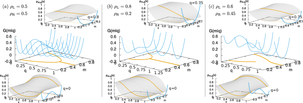
Figure S7: Middle row: Conditional LDF $G(m|q)=G(m,q)-G(q)$ as a function of the mass $m$ for different currents $q$ for three different boundary drivings, namely (a) $\rho_{\text{L}}=0.5,\rho_{\text{R}}=0.5$ (symmetric driving), (b) $\rho_{\text{L}}=0.8,\rho_{\text{R}}=0.2$ (symmetric driving), and (c) $\rho_{\text{L}}=0.6,\rho_{\text{R}}=0.45$ (asymmetric driving). The lines projected in the $m-q$ plane correspond to the local minima of the LDF $G(m|q)$, which define the mass $m_{q}$ associated to a current fluctuation $q$. In the symmetry-broken regime this defines the low- and high-mass branches $m_{q}^{\pm}$. Botton row: optimal density profiles $\rho_{m,q}(x)$ obtained for $q=0$ and the three different boundary drivings. The thick lines are the optimal profiles associated to the local minima $m_{q}^{\pm}$ of $G(m|q)$. For completeness the associated $G(m|q)$ is also shown. Top row: optimal density profiles in each caso, for a current in the PH-symmetric region, $|q|>q_{c}$.

Using this result, it is now possible to study analytically the dynamical phase transition described in the main text for arbitrary boundary gradient (symmetric or asymmetric), well beyond the perturbative nonequilibrium linear regime. In particular, for PH-symmetric boundaries ($\rho_{\text{R}}=1-\rho_{\text{L}}$), the conditional mass-current LDF $G(m|q)\equiv G(m,q)-G(q)$ exhibits a peculiar change of behavior at a critical current $|q_{c}|$, see Figs. S7.a-b: while for $|q|>|q_{c}|$ the LDF $G(m|q)$ displays a single minimum at $m_{q}=1/2$, with an associated PH-symmetric optimal profile (top insets in Figs. S7.a-b), for $|q|<|q_{c}|$ two equivalent minima $m_{q}^{\pm}$ appear in $G(m|q)$, each one associated with a PH-symmetry-broken optimal profile $\rho_{q}^{\pm}(x)$, see bottom insets in Figs. S7.a-b, such that $\rho_{q}^{\pm}(x)\to 1-\rho_{q}^{\mp}(1-x)$. The emergence of this non-convex regime in $G(m|q)$ signals a $2^{\text{nd}}$-order DPT to a PH-symmetry-broken dynamical phase. Note that this happens both for equal boundary densities ($\rho_{\text{R}}=0.5=\rho_{\text{L}}$, Fig. S7.a) and for large but symmetric boundary gradients ($\rho_{\text{L}}=0.8,\rho_{\text{R}}=0.2$, Fig. S7.b). On the other hand, for PH-asymmetric boundaries ($\rho_{\text{R}}\neq 1-\rho_{\text{L}}$, as e.g. $\rho_{\text{L}}=0.6,\rho_{\text{R}}=0.45$, see Fig. S7.c), the governing action (S4) is no longer PH-symmetric: the asymmetry favors one of the mass branches and the associated $G(m|q)$ displays a single global minimum $\forall q$, see Fig. S7.c, and an unique optimal profile. Still, $G(m|q)$ becomes non-convex for low enough currents, and for weak gradient asymmetry, as is the case for $\rho_{\text{L}}=0.6,\rho_{\text{R}}=0.45$ shown in Fig. S7.c, metastable-like local minima in $G(m|q)$ may appear.

The mass $m_{q}$ where the minima of $G(m|q)$ appear for a fixed $q$ is evaluated by demanding $\frac{dG(m|q)}{dm}=\frac{dG(m,q)}{dm}=0$. The $m$-slope of the LDF $G(m,q)$ at a given $(m,q)$-point is simply given by the Lagrange multiplier $\lambda(m,q)$ used to impose the mass constraint, so

$$\frac{dG(m,q)}{dm}\bigg{|}_{m_{q}}=\lambda(m_{q},q)=0\quad\Rightarrow\quad\Lambda_{\text{L}}(m_{q},q,E)=\Lambda_{\text{R}}(m,q,E)\,,$$ (S72)

where we have used the formula which relates the Lagrange multiplier $\lambda(m,q)$ with the boundary slopes $\rho^{\prime}_{\text{L,R}}(m,q,E)$ of the optimal density profile, see Eq. (S22) in §S3 above, with the definition

$$\Lambda_{\text{L,R}}(m,q,E)\equiv\frac{\frac{1}{4}(\rho^{\prime}_{\text{L,R}})^{2}(m,q,E)-q^{2}-E^{2}\rho_{\text{L,R}}^{2}(1-\rho_{\text{L,R}})^{2}}{2\rho_{\text{L,R}}(1-\rho_{\text{L,R}})}\,.$$ (S73)

In this way, defining $\sigma_{\text{L,R}}\equiv\rho_{\text{L,R}}(1-\rho_{\text{L,R}})$, the equation for the mass minima $m_{q}$ for a fixed $q$ is

$$\frac{1}{4\sigma_{\text{L}}}(\rho^{\prime}_{\text{L}})^{2}(m_{q},q,E)-\frac{1}{4\sigma_{\text{R}}}(\rho^{\prime}_{\text{R}})^{2}(m_{q},q,E)=q^{2}\left(\frac{1}{\sigma_{\text{L}}}-\frac{1}{\sigma_{\text{R}}}\right)+E^{2}(\sigma_{\text{L}}-\sigma_{\text{R}})\,.$$ (S74)

The critical current $q_{c}$ can be evaluated as well by demanding that

$$\frac{dG(m,q)}{dm}\bigg{|}_{m_{q_{c}},q_{c}}=0=\frac{d^{2}G(m,q)}{dm^{2}}\bigg{|}_{m_{q_{c}},q_{c}}\,,$$ (S75)

which leads to the following pair of equations

$$\frac{1}{4\sigma_{\text{L}}}(\rho^{\prime}_{\text{L}})^{2}(m_{q_{c}},q_{c},E)-\frac{1}{4\sigma_{\text{R}}}(\rho^{\prime}_{\text{R}})^{2}(m_{q_{c}},q_{c},E) = q_{c}^{2}\left(\frac{1}{\sigma_{\text{L}}}-\frac{1}{\sigma_{\text{R}}}\right)+E^{2}(\sigma_{\text{L}}-\sigma_{\text{R}})\,,$$ (S76)

$$\frac{\rho^{\prime}_{\text{L}}(m,q,E)}{\sigma_{\text{L}}}\frac{d\rho^{\prime}_{\text{L}}(m,q,E)}{dm}\bigg{|}_{m_{q_{c}},q_{c}} = \frac{\rho^{\prime}_{\text{R}}(m,q,E)}{\sigma_{\text{R}}}\frac{d\rho^{\prime}_{\text{R}}(m,q,E)}{dm}\bigg{|}_{m_{q_{c}},q_{c}}\,.$$ (S77)

Note that these equations for $m_{q}$ and for $q_{c}$ must be solved numerically due to the nonlinear character of the problem.

S4 Instanton solution, Maxwell-like construction and violation of additivity principle

In this section we build a time-dependent, instanton-like solution for the optimal density and current fields responsible of a joint fluctuation of the empirical current and mass. We further show that this solution improves the additivity principle prediction (i.e. yields a better minimizer of the MFT action) in the regime where the joint current-mass LDF becomes non-convex. This result demonstrates that time-dependent solutions of the MFT problem in open systems exist and dominate fluctuation behavior in dynamical coexistence regimes emerging at DPTs.

We start from the general expression derived above for the joint mass-current LDF, see Eq. (S7),

$$G(m,q)=\lim_{\tau\rightarrow\infty}\frac{1}{\tau}\min_{\{\rho,j\}_{0}^{\tau}}\int_{0}^{\tau}dt\int_{0}^{1}dx\frac{[j+D(\rho)\partial_{x}\rho-E\sigma(\rho)]^{2}}{2\sigma(\rho)}\,,$$ (S78)

with the fields $\rho(x,t)$ and $j(x,t)$ coupled at every point of space and time via the continuity equation, $\partial_{t}\rho+\partial_{x}j=0$. Moreover, the density and current fields are further constrained to yield empirical values

$$q = \frac{1}{\tau}\int_{0}^{\tau}dt\int_{0}^{1}dx\,j(x,t)\,,$$ (S79)

$$m = \frac{1}{\tau}\int_{0}^{\tau}dt\int_{0}^{1}dx\,\rho(x,t)\,,$$ (S80)

and boundary conditions for the density field are such that $\rho(0,t)=\rho_{\text{L}}$ and $\rho(1,t)=\rho_{\text{R}}$ $\forall t$. We have seen in previous sections of the SM that, under the additivity conjecture Bodineau and Derrida (2004), the joint mass-current LDF is simplified to

$$G_{\text{ad}}(m,q)=\min_{\rho(x)}\int_{0}^{1}dx\frac{\displaystyle\left[q+D(\rho)\rho^{\prime}(x)-\sigma(\rho)E\right]^{2}}{\displaystyle 2\sigma(\rho)}\,,$$ (S81)

with a reduced set of constraints (i.e. boundary densities, and total mass). We denote in this section as $\rho_{m,q}^{\text{ad}}(x)$ the optimal density profile responsible of a joint mass and current fluctuation under the additivity hypothesis. To search for violations of the additivity principle, we focus our attention in current fluctuations $|q|\leq q_{c}$ below the critical point in systems driven by a symmetric density gradient ($\rho_{\text{R}}=1-\rho_{\text{L}}$). In this regime we conjecture a solution for the optimal trajectory responsible of a given mass-current fluctuation, which is time-dependent for masses where $G(m,q)$ is non-convex. In particular, our ansatz in this regime is

$$\rho_{m,q}(x,t)=\left\{\begin{array}[]{ll}\rho_{m,q}^{\text{ad}}(x)&\text{if }m<m_{q}^{-}\text{ or }m>m_{q}^{+}\\ \phantom{aaa}&\phantom{bbb}\\ \rho_{m_{q}^{-},q}^{\text{ad}}(x)\left[1-\phi(t-t_{m,q})\right]+\rho_{m_{q}^{+},q}^{\text{ad}}(x)~{}\phi(t-t_{m,q})&\text{if }m_{q}^{-}\leq m\leq m_{q}^{+}\end{array}\right.$$ (S82)

where $m_{q}^{\pm}$ are the masses of the optimal density profiles associated to a current fluctuation $|q|\leq q_{c}$ in the PH symmetry broken regime along the high-mass ($+$) and low-mass ($-$) branches. The time-dependent function $\phi(t)$ is a sufficiently smooth localized crossover function such that $\phi(t)=0$ $\forall t<-\frac{\delta t}{2}$ and $\phi(t)=1$ $\forall t>\frac{\delta t}{2}$, with $\delta t$ a fixed timescale. The crossover time $t_{m,q}$ in Eq (S82) can be determined now by imposing the constraint on the empirical mass, Eq. (S80). In particular

$$m = \frac{1}{\tau}\int_{0}^{\tau}dt\int_{0}^{1}dx\,\rho_{m,q}(x,t)=\left(\frac{t_{m,q}-\frac{\delta t}{2}}{\tau}\right)m_{q}^{-}+\left(\frac{\tau-(t_{m,q}+\frac{\delta t}{2})}{\tau}\right)m_{q}^{+}+\frac{1}{\tau}\int_{t_{m,q}-\frac{\delta t}{2}}^{t_{m,q}+\frac{\delta t}{2}}dt\int_{0}^{1}dx\rho_{m,q}(x,t)$$ (S83)

$$= \frac{t_{m,q}}{\tau}m_{q}^{-}+\left(1-\frac{t_{m,q}}{\tau}\right)m_{q}^{+}+\frac{1}{\tau}\left[-\delta t+\int_{t_{m,q}-\frac{\delta t}{2}}^{t_{m,q}+\frac{\delta t}{2}}dt\int_{0}^{1}dx\rho_{m,q}(x,t)\right]\,.$$

The third term in the rhs of the last equation is $\sim{\cal O}(\delta t/\tau)$, so in the long-time limit ($\tau\to\infty$) and for a fixed crosscover time $\delta t$ this term tends to zero, and hence we find $t_{m,q}=p~{}\tau$ with the definition

$$p=\frac{m_{q}^{+}-m}{m_{q}^{+}-m_{q}^{-}}\,.$$ (S84)

As mentioned above, the time-dependent optimal density field $\rho_{m,q}(x,t)$ must obey at all points of space and time a continuity equation $\partial_{t}\rho_{m,q}(x,t)+\partial_{x}j_{m,q}(x,t)=0$. To obtain the optimal time-dependent current field $j_{m,q}(x,t)$ for $m_{q}^{-}\leq m\leq m_{q}^{+}$, we first note that in this case

$$\partial_{t}\rho_{m,q}(x,t)=\left\{\begin{array}[]{ll}0&\text{if }t\notin[t_{m,q}-\frac{\delta t}{2},t_{m,q}+\frac{\delta t}{2}]\\ \phantom{aaa}&\phantom{bbb}\\ \left[\rho_{m_{q}^{+},q}^{\text{ad}}(x)-\rho_{m_{q}^{-},q}^{\text{ad}}(x)\right]~{}\phi^{\prime}(t-t_{m,q})&\text{if }t\in[t_{m,q}-\frac{\delta t}{2},t_{m,q}+\frac{\delta t}{2}]\end{array}\right.$$ (S85)

Therefore the continuity constraint in the mass regime $m_{q}^{-}\leq m\leq m_{q}^{+}$ leads to the following optimal current trajectory

$$j_{m,q}(x,t)=\left\{\begin{array}[]{ll}q&\text{if }t\notin[t_{m,q}-\frac{\delta t}{2},t_{m,q}+\frac{\delta t}{2}]\\ \phantom{aaa}&\phantom{bbb}\\ \chi(x)~{}\phi^{\prime}(t-t_{m,q})&\text{if }t\in[t_{m,q}-\frac{\delta t}{2},t_{m,q}+\frac{\delta t}{2}]\end{array}\right.$$ (S86)

where we have already taken into account the constraint on the empirical current $q$, see Eq. (S79). The function $\chi(x)$ is such that $\chi^{\prime}(x)=\rho_{m_{q}^{+},q}^{\text{ad}}(x)-\rho_{m_{q}^{-},q}^{\text{ad}}(x)$, and we note that the transient regime where $j_{m,q}(x,t)$ is different from $q$ does not contribute to the final value of the empirical current, Eq. (S79), as this transient is negligible against the long-time limit for $\tau$.

Using this ansatz for the optimal trajectory responsible of a mass and current fluctuation in Eq. (S78), we obtain for the associated joint LDF

$$G(m,q) = \lim_{\tau\rightarrow\infty}\frac{1}{\tau}\int_{0}^{\tau}dt\int_{0}^{1}dx\frac{[j_{m,q}(x,t)+D(\rho_{m,q})\partial_{x}\rho_{m,q}(x,t)-E\sigma(\rho_{m,q})]^{2}}{2\sigma(\rho_{m,q})}$$ (S87)

$$= \lim_{\tau\rightarrow\infty}\left[\left(\frac{t_{m,q}-\frac{\delta t}{2}}{\tau}\right)G_{\text{ad}}(m_{q}^{-},q)+\left(\frac{\tau-(t_{m,q}+\frac{\delta t}{2})}{\tau}\right)G_{\text{ad}}(m_{q}^{+},q)+\frac{1}{\tau}{\cal I}\right]\,,$$

with the definition

$${\cal I}\equiv\int_{t_{m,q}-\frac{\delta t}{2}}^{t_{m,q}+\frac{\delta t}{2}}dt\int_{0}^{1}dx\frac{[j_{m,q}(x,t)+D(\rho_{m,q})\partial_{x}\rho_{m,q}(x,t)-E\sigma(\rho_{m,q})]^{2}}{2\sigma(\rho_{m,q})}\,.$$ (S88)

Noting that ${\cal I}\sim{\cal O}(\delta t)$ and using the same arguments as above, we find in the long-time limit $\tau\to\infty$ that

$$G(m,q)=p~{}G_{\text{ad}}(m_{q}^{-},q)+(1-p)G_{\text{ad}}(m_{q}^{+},q)\,,$$ (S89)

which corresponds to the Maxwell construction obtained from $G_{\text{ad}}(m,q)$ in the mass regime $m_{q}^{-}\leq m\leq m_{q}^{+}$ where this joint LDF is non-convex (for $|q|\leq q_{c}$), as described above and in the main text. Note that an equivalent argument can be developed for the conditional mass-current LDF $G(m|q)=G(m,q)-G(q)$. This instanton solution corresponds to the dynamical coexistence of the different symmetry-broken phases which appear for $|q|\leq q_{c}$, a behavior typical of $1^{\text{st}}$-order DPTs. Note also that one can generalize the previous solution to PH-asymmetric boundaries in regimes where $G(m,q)$ is non-convex. Finally, we would like to mention that some subtleties of the instanton solution appear for $|q|\approx q_{c}$ related to the order of the $L\to\infty$ and $\tau\to\infty$ limits, see Ref. Baek et al. (2018) for a discussion of this issue.

S5 Spectral analysis of the dynamical generator and metastable manifold

In this section we perform a spectral analysis of the microscopic dynamics of the $1d$ WASEP in order to better understand the DPT demonstrated above from a microscopic point of view. In particular, we will focus on the quasi-degenerate (metastable) states $\left|P_{MS}^{c_{1}}\right\rangle$ and $\left|P_{MS}^{c_{2}}\right\rangle$ introduced in the main text, which contain the information about the optimal trajectories in the symmetry-broken phase.

At the microscopic level, a configuration of the $1d$ WASEP is given by $C=\{n_{k}\}_{k=1,\ldots,L}$, where $n_{k}=0,1$ is the occupation number of the $k^{\text{th}}$-site of the lattice. Within the quantum Hamiltonian formalism for the master equation Schutz (2001), each configuration is then represented as a vector in a Hilbert space

$$\left|C\right\rangle=\bigotimes_{k=1}^{L}\begin{pmatrix}n_{k}\\ 1-n_{k}\end{pmatrix}\,,$$ (S90)

and the complete information about the system is contained in a vector $\left|P\right\rangle=(P(C_{1}),P(C_{2}),...)^{T}=\sum_{i}P(C_{i})\left|C_{i}\right\rangle$, with ^T denoting transposition, such that $P(C_{i})$ represents the probability of configuration $C_{i}$. This probability vector is normalized such that $\langle-|P\rangle=1$ where $\left\langle-\right|=\sum_{i}\left\langle C_{i}\right|$ is the vector representing the sum over all possible configurations and $\langle C_{i}|C_{j}\rangle=\delta_{ij}$. The probability vector $\left|P\right\rangle$ evolves in time according to the master equation

$$\partial_{t}\left|P\right\rangle={\mathbb{W}}\left|P\right\rangle\,,$$ (S91)

where ${\mathbb{W}}$ defines the Markov generator of the dynamics. Such generator can be tilted ${\mathbb{W}}^{\mu,\lambda}$Touchette (2009); Hurtado et al. (2014) to bias the original stochastic dynamics in order to favor large (low) mass for $\mu<0$ ($\mu>0$) and large (low) currents for $\lambda>0$ ($\lambda<0$), with $\mu$ and $\lambda$ the conjugate parameters to the microscopic mass and current observables, respectively. In particular, the tilted dynamical generator for the $1d$ open WASEP is

$${\mathbb{W}}^{\mu,\lambda} = \sum_{k=1}^{L-1}[\frac{1}{2}e^{(\lambda+E)/(L-1)}\sigma_{k+1}^{+}\sigma_{k}^{-}+\frac{1}{2}e^{-(\lambda+E)/(L-1)}\sigma_{k}^{+}\sigma_{k+1}^{-}$$ (S92)

$$- \frac{1}{2}e^{E/(L-1)}{\hat{n}}_{k}({\mathbb{1}}-{\hat{n}}_{k+1})-\frac{1}{2}e^{-E/(L-1)}{\hat{n}}_{k+1}({\mathbb{1}}-{\hat{n}}_{k})]$$

$$+ \alpha[\sigma_{1}^{+}-({\mathbb{1}}-{\hat{n}}_{1})]+\gamma[\sigma_{1}^{-}-{\hat{n}}_{1}]$$

$$+ \delta[\sigma_{L}^{+}-({\mathbb{1}}-{\hat{n}}_{L})]+\beta[\sigma_{L}^{-}-{\hat{n}}_{L}]-\frac{\mu}{L}\sum_{k=1}^{L}{\hat{n}}_{k}\,,$$

and we recall (see main text) that $\alpha$ and $\gamma$ ($\delta$ and $\beta$) are the injection and extraction rates at the leftmost (rightmost) site, respectively. In the previous expression ${\mathbb{1}}$ is the identity matrix and ${\hat{n}}_{k}=\sigma_{k}^{+}\sigma_{k}^{-}$ is the number operator at site $k\in[1,L]$, where $\sigma_{k}^{+}$ and $\sigma_{k}^{-}$ are the creation and annihilation operators given by $\sigma_{k}^{\pm}=(\sigma_{k}^{x}\pm i\sigma_{k}^{y})/2$ respectively, with $\sigma_{k}^{x,y}$ the standard $x,y$-Pauli matrices acting on site $k$. The connection between the biased dynamics and the large deviation properties of the $1d$ WASEP is established through the largest eigenvalue of ${\mathbb{W}}^{\mu,\lambda}$ Touchette (2009); Garrahan (2018). Such eigenvalue, denoted by $\theta_{0}(\mu,\lambda)$, is nothing but the cumulant generating function of the observables $m$ and $q$, related to the LDF $G(m,q)$ via a Legendre transform,

$$\theta_{0}(\mu,\lambda)=L^{-1}\max_{m,q}[\lambda q-\mu Lm-G(m,q)]\,.$$ (S93)

The average of an observable $b$ at a final time $t$ in the unbiased ($\lambda=\mu=0$) dynamics can be written in operator notation as $\langle b(t)\rangle\equiv\langle-|\hat{b}e^{t\!~{}{\mathbb{W}}^{0,0}}|P_{0}\rangle$. We can write the time evolution operator for long times as $e^{t\!~{}{\mathbb{W}}^{0,0}}\sim\left|P_{ss}\right\rangle\left\langle-\right|$, with $\left|P_{ss}\right\rangle$ being the stationary state probability vector. Thus, as $\langle-|P_{0}\rangle=1$ the average of $b$ is $\langle b(t)\rangle\equiv\langle-|\hat{b}\left|P_{ss}\right\rangle$. Since we are in the unbiased dynamics this average is the same at both the final time $t$ and the intermediate times $0\ll\tau\ll t$, so that $\langle b(t)\rangle=\langle b(\tau)\rangle$ Garrahan et al. (2009). However, for a biased dynamics such as ${\mathbb{W}}^{0,\lambda}$, we are interested in computing the average of observables at intermediate times, since the rare event sustained by ${\mathbb{W}}^{0,\lambda}$ presents time-boundary effects which make the average at final and at intermediate times no longer equivalent Garrahan et al. (2009). Hence, in order to make these averages equivalent in the biased dynamics, we transform the non-stochastic generator ${\mathbb{W}}^{0,\lambda}$ (note that it does not conserve probability $\left\langle-\right|{\mathbb{W}}^{0,\lambda}\neq 0$) into a physical stochastic generator via the Doob transform Chetrite and Touchette (2015a); Carollo et al. (2018b):

$${\mathbb{W}}^{0,\lambda}_{Doob}=\hat{L}_{0}{\mathbb{W}}^{0,\lambda}\hat{L}_{0}^{-1}-\theta_{0}(\lambda)\,,$$ (S94)

which is a proper stochastic generator (now $\left\langle-\right|{\mathbb{W}}^{0,\lambda}_{Doob}=0$), with largest eigenvalue equal to zero, generating the same trajectories as ${\mathbb{W}}^{0,\lambda}$. Here $\hat{L}_{0}$ is a diagonal matrix whose elements $(\hat{L}_{0})_{ii}$ are the $i$-th entries of the left eigenvector $\left\langle L_{0}\right|$ of the biased generator ${\mathbb{W}}^{0,\lambda}$ associated with its largest eigenvalue $\theta_{0}(\lambda)$. Thus, with this new generator ${\mathbb{W}}^{0,\lambda}_{Doob}$ we can compute the average of any observable $b$ at intermediate times as

$$\langle b(\tau)\rangle_{\lambda}=\langle b(t)\rangle_{\lambda}\equiv\frac{\langle-|\hat{b}e^{t\!~{}{\mathbb{W}}^{0,\lambda}_{Doob}}|P_{0}\rangle}{\langle-|e^{t\!~{}{\mathbb{W}}^{0,\lambda}_{Doob}}|P_{0}\rangle}\,.$$ (S95)

In what follows we show how the previous average takes different forms depending on whether or not the largest eigenvalue of the biased generator ${\mathbb{W}}^{0,\lambda}$ is degenerate.

S5.1 Non-degenerate largest eigenvalue (PH symmetric phase)

If $\theta_{0}(\lambda)$ is non-degenerate, the time evolution operator for long times is $e^{t\!~{}{\mathbb{W}}^{0,\lambda}}\sim e^{t\theta_{0}(\lambda)}\left|R_{0}\right\rangle\left\langle L_{0}\right|$. Then by using (S94) the asymptotic Doob time evolution operator reads

$$e^{t\!~{}{\mathbb{W}}^{0,\lambda}_{Doob}}\sim\hat{L}_{0}\left|R_{0}\right\rangle\left\langle L_{0}\right|\hat{L}_{0}^{-1}=\hat{L}_{0}\left|R_{0}\right\rangle\left\langle-\right|\,,$$

with $\left|R_{0}\right\rangle$ being the right eigenvector of ${\mathbb{W}}^{0,\lambda}$ associated with its largest eigenvalue $\theta_{0}(\lambda)$. Additionally we can normalize eigenvectors so that

$$\langle L_{i}|R_{j}\rangle=\delta_{ij}~{}~{}~{}~{}~{}\text{and}~{}~{}~{}~{}~{}\langle-|R_{0}\rangle=1\,.$$

Thus the time-evolved initial probability vector is

$$e^{t\!~{}{\mathbb{W}}^{0,\lambda}_{Doob}}|P_{0}\rangle\sim\hat{L}_{0}\left|R_{0}\right\rangle\,.$$ (S96)

As a consequence the average (S95) is given by

$$\langle b(\tau)\rangle_{\lambda}=\frac{\langle-|\hat{b}\hat{L}_{0}\left|R_{0}\right\rangle}{\langle-|\hat{L}_{0}\left|R_{0}\right\rangle}=\frac{\langle-|\hat{b}\hat{L}_{0}\left|R_{0}\right\rangle}{\langle L_{0}|R_{0}\rangle}=\langle-|\hat{b}\hat{L}_{0}\left|R_{0}\right\rangle$$

where in the last equality we have used the fact that eigenvectors are normalized. This is how we calculate, from the microscopic dynamics, the optimal density profiles associated with current fluctuations ($\lambda\neq 0$) in the particle-hole (PH) symmetric phase. The optimal particle density in the large size limit at $x=k/L$, with $L$ being the total number of sites, is thus given by

$$\rho(x)=\langle\hat{n}_{k}(\tau)\rangle_{\lambda}=\langle-|\hat{n}_{k}\hat{L}_{0}\left|R_{0}\right\rangle\,.$$

S5.2 Degenerate largest eigenvalue (PH symmetry-broken phase)

As we have seen in the main text, for $\lambda_{c}^{-}\leq\lambda\leq\lambda_{c}^{+}$ (or equivalently $|q|\leq q_{c}$), the largest eigenvalue of ${\mathbb{W}}^{0,\lambda}$ becomes degenerate in the large size limit, $L\to\infty$. This is reflected in the diffusively-scaled spectral gap, $L^{2}[\theta_{0}(0,\lambda)-\theta_{1}(0,\lambda)]$, with $\theta_{1}(0,\lambda)$ the next-to-leading eigenvalue of ${\mathbb{W}}^{0,\lambda}$, which tends to zero as $L$ increases in this $\lambda$-region. In this case, defining as $\left|R_{1}\right\rangle$ and $\left\langle L_{1}\right|$ the right and left eigenvectors associated to $\theta_{1}(0,\lambda)$, we have that the time evolution operator can be written for long times as $e^{t\!~{}{\mathbb{W}}^{0,\lambda}}\sim e^{t\theta_{0}(\lambda)}(\left|R_{0}\right\rangle\left\langle L_{0}\right|+\left|R_{1}\right\rangle\left\langle L_{1}\right|)$. Hence, by using (S94) the asymptotic Doob time evolution operator reads

$$e^{t\!~{}{\mathbb{W}}^{0,\lambda}_{Doob}}\sim\hat{L}_{0}\left|R_{0}\right\rangle\left\langle L_{0}\right|L_{0}^{-1}+\hat{L}_{0}\left|R_{1}\right\rangle\left\langle L_{1}\right|\hat{L}_{0}^{-1}=\hat{L}_{0}\left|R_{0}\right\rangle\left\langle-\right|+\hat{L}_{0}\left|R_{1}\right\rangle\left\langle L_{1}\right|\hat{L}_{0}^{-1}\,.$$

Thus the time-evolved initial vector probability is

$$\boxed{e^{t\!~{}{\mathbb{W}}^{0,\lambda}_{Doob}}|P_{0}\rangle\sim\hat{L}_{0}\left|R_{0}\right\rangle+c\hat{L}_{0}\left|R_{1}\right\rangle\,}\,,$$ (S97)

with $c=\left\langle L_{1}\right|\hat{L}_{0}^{-1}|P_{0}\rangle$. Note that, since $\langle-|P_{0}\rangle=1$ then $c\in[c_{1},c_{2}]$ with $c_{1}=\min\left(\left\langle L_{1}\right|\hat{L}_{0}^{-1}\right)$ and $c_{2}=\max\left(\left\langle L_{1}\right|\hat{L}_{0}^{-1}\right)$, where $\min$ and $\max$ correspond to the minimum and maximum entries of the vector $\left\langle L_{1}\right|\hat{L}_{0}^{-1}$. Thus, Eq. (S97) defines the set of metastable states $|P_{MS}^{c}\rangle$ of the main text, whose extremes are given by $|P_{MS}^{c_{1}}\rangle$ and $|P_{MS}^{c_{2}}\rangle$. As a consequence the average (S95) is given by

$$\langle b(\tau)\rangle_{\lambda}=\frac{\langle-|\hat{b}\hat{L}_{0}\left|R_{0}\right\rangle+c\langle-|\hat{b}\hat{L}_{0}\left|R_{1}\right\rangle}{\langle-|\hat{L}_{0}\left|R_{0}\right\rangle+c\langle-|\hat{L}_{0}\left|R_{1}\right\rangle}=\langle-|\hat{b}\hat{L}_{0}\left|R_{0}\right\rangle+c\langle-|\hat{b}\hat{L}_{0}\left|R_{1}\right\rangle$$

where in the last equality we have used the fact that eigenvectors are normalized. This is how we calculate, from the microscopic dynamics, the optimal density profiles associated with current fluctuations ($\lambda\neq 0$) in the symmetry-broken phase. The optimal particle densities in the large size limit at $x=k/L$, are thus given by

$$\rho_{1}(x)=\langle\hat{n}_{k}(\tau)\rangle_{\lambda}=\langle-|\hat{n}_{k}\hat{L}_{0}\left|R_{0}\right\rangle+c_{1}\langle-|\hat{n}_{k}\hat{L}_{0}\left|R_{1}\right\rangle\,$$

and

$$\rho_{2}(x)=\langle\hat{n}_{k}(\tau)\rangle_{\lambda}=\langle-|\hat{n}_{k}\hat{L}_{0}\left|R_{0}\right\rangle+c_{2}\langle-|\hat{n}_{k}\hat{L}_{0}\left|R_{1}\right\rangle\,,$$

which correspond to the metastable density profiles for $L=10$ and $L=20$ of Fig. 4 in the main text.

References

Bertini et al. (2005)L. Bertini, A. De Sole,
D. Gabrielli, G. Jona-Lasinio, and C. Landim, “Current fluctuations in stochastic lattice
gases,” Phys. Rev. Lett. 94, 030601 (2005).
Bodineau and Derrida (2005)T. Bodineau and B. Derrida, “Distribution of
current in nonequilibrium diffusive systems and phase transitions,” Phys. Rev. E 72, 066110 (2005).
Harris et al. (2005)R. J. Harris, A. Rakos, and G. M. Schutz, “Current fluctuations in the
zero-range process with open boundaries,” J. Stat. Mech. , P08003 (2005).
Bertini et al. (2006)L. Bertini, A. De Sole,
D. Gabrielli, G. Jona-Lasinio, and C. Landim, “Nonequilibrium current fluctuations in
stochastic lattice gases,” J. Stat. Phys. 123, 237–276 (2006).
Bodineau and Derrida (2007)T. Bodineau and B. Derrida, “Cumulants and
large deviations of the current through non-equilibrium steady states,” C.R. Phys. 8, 540 – 555 (2007).
Lecomte et al. (2007)V. Lecomte, C. Appert-Rolland, and F. van Wijland, “Thermodynamic formalism for systems with Markov dynamics,” J. Stat. Phys. 127, 51 (2007).
Garrahan et al. (2007)J. P. Garrahan, R. L. Jack,
V. Lecomte, E. Pitard, K. van Duijvendijk, and F. van Wijland, “Dynamical first-order phase transition in
kinetically constrained models of glasses,” Phys. Rev. Lett. 98, 195702 (2007).
Garrahan et al. (2009)J. P. Garrahan, R. L. Jack,
V. Lecomte, E. Pitard, K. van Duijvendijk, and F. van Wijland, “First-order dynamical phase transition in models
of glasses: an approach based on ensembles of histories,” J. Phys. A 42, 075007 (2009).
Hurtado and Garrido (2011)P. I. Hurtado and P. L. Garrido, “Spontaneous
symmetry breaking at the fluctuating level,” Phys. Rev. Lett. 107, 180601 (2011).
Ates et al. (2012)C. Ates, B. Olmos,
J. P. Garrahan, and I. Lesanovsky, “Dynamical phases and intermittency of
the dissipative quantum Ising model,” Phys. Rev. A 85, 043620 (2012).
Pérez-Espigares et al. (2013)C. Pérez-Espigares, P. L. Garrido, and P. I. Hurtado, “Dynamical phase
transition for current statistics in a simple driven diffusive system,” Phys. Rev. E 87, 032115 (2013).
Harris et al. (2013)R. J. Harris, V. Popkov, and G. M. Schütz, “Dynamics of instantaneous
condensation in the ZRP conditioned on an atypical current,” Entropy 15, 5065
(2013).
Vaikuntanathan et al. (2014)S. Vaikuntanathan, T. R. Gingrich, and P. L. Geissler, “Dynamic phase
transitions in simple driven kinetic networks,” Phys. Rev. E 89, 062108 (2014).
Mey et al. (2014)A. S. J. S. Mey, P. L. Geissler, and J. P. Garrahan, “Rare-event
trajectory ensemble analysis reveals metastable dynamical phases in lattice
proteins,” Physical Review E 89, 032109 (2014).
Jack et al. (2015)R. L. Jack, I. R. Thompson,
and P. Sollich, “Hyperuniformity and phase
separation in biased ensembles of trajectories for diffusive systems,” Phys. Rev. Lett. 114, 060601 (2015).
Nyawo and Touchette (2016)O. Tsobgni Nyawo and H. Touchette, “A minimal model of dynamical phase transition,” Europhys. Lett. 116, 50009 (2016).
Harris and Touchette (2017)R. J. Harris and H. Touchette, “Phase
transitions in large deviations of reset processes,” J. Phys. A 50, 10LT01 (2017).
Lazarescu (2017)A. Lazarescu, “Generic
dynamical phase transition in one-dimensional bulk-driven lattice gases with
exclusion,” J. Phys. A 50, 254004 (2017).
Brandner et al. (2017)K. Brandner, V.F. Maisi,
J.P. Pekola, J.P. Garrahan, and C. Flindt, “Experimental determination of dynamical
Lee-Yang zeros,” Phys. Rev. Lett. 118 (2017).
Karevski and Schütz (2017)D. Karevski and G.M. Schütz, “Conformal
invariance in driven diffusive systems at high currents,” Phys. Rev. Lett. 118 (2017).
Carollo et al. (2017)F. Carollo, J. P. Garrahan, I. Lesanovsky, and C. Pérez-Espigares, “Fluctuating hydrodynamics, current fluctuations, and hyperuniformity in
boundary-driven open quantum chains,” Phys.
Rev. E 96, 052118
(2017).
Baek et al. (2017)Y. Baek, Y. Kafri, and V. Lecomte, “Dynamical symmetry breaking and phase
transitions in driven diffusive systems,” Phys. Rev. Lett. 118, 030604 (2017).
Tizón-Escamilla et al. (2017)N. Tizón-Escamilla, C. Pérez-Espigares, P. L. Garrido, and P. I. Hurtado, “Order and
symmetry breaking in the fluctuations of driven systems,” Phys. Rev. Lett. 119, 090602 (2017).
Shpielberg (2017)O. Shpielberg, “Geometrical
interpretation of dynamical phase transitions in boundary-driven systems,” Phys. Rev. E 96, 062108 (2017).
Baek et al. (2018)Y. Baek, Y. Kafri, and V. Lecomte, “Dynamical phase transitions in the
current distribution of driven diffusive channels,” J. Phys. A 51, 105001 (2018).
Shpielberg et al. (2018)O. Shpielberg, T. Nemoto,
and J. Caetano, “Universality in dynamical
phase transitions of diffusive systems,” Phys.
Rev. E 98, 052116
(2018).
Pérez-Espigares et al. (2018)C. Pérez-Espigares, I. Lesanovsky, J. P. Garrahan, and R. Gutiérrez, “Glassy
dynamics due to a trajectory phase transition in dissipative rydberg
gases,” Phys. Rev. A 98, 021804 (2018).
Chleboun et al. (2018)P. Chleboun, S. Grosskinsky, and A. Pizzoferrato, “Current
large deviations for partially asymmetric particle systems on a ring,” J. Phys. A 51, 405001 (2018).
Klymko et al. (2018)K. Klymko, P. L. Geissler, J. P. Garrahan, and S. Whitelam, “Rare behavior
of growth processes via umbrella sampling of trajectories,” Phys. Rev. E 97, 032123 (2018).
Whitelam (2018)S. Whitelam, “Large
deviations in the presence of cooperativity and slow dynamics,” Phys. Rev. E 97, 062109 (2018).
Vroylandt and Verley (2018)H. Vroylandt and G. Verley, “Non equivalence
of dynamical ensembles and emergent non ergodicity,” arXiv:1806.11470 (2018).
Binney et al. (1992)J. J. Binney, N. J. Dowrick,
A. J. Fisher, and M. Newman, The Theory of Critical Phenomena: An Introduction
to the Renormalization Group (Oxford University
Press, Inc., New York, NY, USA, 1992).
Zinn-Justin (2002)J. Zinn-Justin, Quantum Field
Theory and Critical Phenomena; 4th ed., Internat. Ser. Mono. Phys. (Clarendon Press, Oxford, 2002).
(35)B. Derrida, “Non-equilibrium
steady states: fluctuations and large deviations of the density and of the
current,” J. Stat. Mech. P07023 (2007) .
Hurtado et al. (2014) P. I. Hurtado, C. P. Espigares, J. J. del Pozo, and P. L. Garrido, “Thermodynamics of currents in nonequilibrium diffusive systems: theory and
simulation,” J. Stat. Phys. 154, 214–264 (2014).
Lazarescu (2015)A. Lazarescu, “The
physicist’s companion to current fluctuations: one-dimensional bulk-driven
lattice gases,” J. Phys. A 48, 503001 (2015).
Carollo et al. (2018a)F. Carollo, J. P. Garrahan, and I. Lesanovsky, “Current
fluctuations in boundary-driven quantum spin chains,” Phys.
Rev. B 98, 094301
(2018a).
Touchette (2009)H. Touchette, “The large
deviation approach to statistical mechanics,” Phys. Rep. 478, 1–69 (2009).
Bertini et al. (2015)L. Bertini, A. De Sole,
D. Gabrielli, G. Jona-Lasinio, and C. Landim, “Macroscopic fluctuation theory,” Rev. Mod. Phys. 87, 593–636 (2015).
Hedges et al. (2009)L. O. Hedges, R. L. Jack,
J. P. Garrahan, and D. Chandler, “Dynamic order-disorder in atomistic
models of structural glass formers,” Science 323, 1309 (2009).
Chandler and Garrahan (2010)D. Chandler and J. P. Garrahan, “Dynamics on
the way to forming glass: bubbles in space-time.” Annu. Rev. Phys. Chem. 61, 191–217 (2010).
Pitard et al. (2011)E. Pitard, V. Lecomte, and F. Van Wijland, “Dynamic transition in an
atomic glass former: A molecular-dynamics evidence,” Europhys. Lett. 96, 56002 (2011).
Speck et al. (2012)T. Speck, A. Malins, and C. P. Royall, “First-order phase transition
in a model glass former: Coupling of local structure and dynamics,” Phys. Rev. Lett. 109, 195703 (2012).
Pinchaipat et al. (2017)R. Pinchaipat, M. Campo,
F. Turci, J. Hallett, T. Speck, and C. P. Royall, “Experimental evidence for a structural-dynamical
transition in trajectory space,” Phys. Rev. Lett. 119, 028004 (2017).
Abou et al. (2018)B. Abou, R. Colin,
V. Lecomte, E. Pitard, and F. van Wijland, “Activity statistics in a colloidal glass former:
experimental evidence for a dynamical transition,” J.Chem. Phys. 148, 164502 (2018).
Garrahan et al. (2011)J. P. Garrahan, A. D. Armour, and I. Lesanovsky, “Quantum
trajectory phase transitions in the micromaser,” Phys. Rev. E 84, 021115 (2011).
Genway et al. (2012)S. Genway, J. P. Garrahan, I. Lesanovsky, and A. D. Armour, “Phase
transitions in trajectories of a superconducting single-electron transistor
coupled to a resonator,” Phys. Rev. E 85, 051122 (2012).
Manzano and Hurtado (2014)D. Manzano and P. I. Hurtado, “Symmetry and
the thermodynamics of currents in open quantum systems,” Phys. Rev. B 90, 125138 (2014).
Manzano and Kyoseva (2016)D. Manzano and E. Kyoseva, “An atomic
symmetry-controlled thermal switch,” Sci. Rep. 6, 31161 (2016).
Manzano and Hurtado (2018)D. Manzano and P.I. Hurtado, “Harnessing
symmetry to control quantum transport,” Adv. in Phys. 67, 1
(2018).
Chetrite and Touchette (2015a)R. Chetrite and H. Touchette, “Variational
and optimal control representations of conditioned and driven processes,” J. Stat. Mech. P12001
(2015a).
Chetrite and Touchette (2015b)R. Chetrite and H. Touchette, “Nonequilibrium Markov processes conditioned on large deviations,” Ann. Henri Poincare 16, 2005 (2015b).
Carollo et al. (2018b)F. Carollo, J. P. Garrahan, I. Lesanovsky, and C. Pérez-Espigares, “Making rare events typical in Markovian open quantum systems,” Phys. Rev. A 98, 010103 (2018b).
Bodineau and Derrida (2004)T. Bodineau and B. Derrida, “Current
fluctuations in nonequilibrium diffusive systems: An additivity
principle,” Phys. Rev. Lett. 92, 180601 (2004).
Gärtner (1987)J. Gärtner, “Convergence
towards burger’s equation and propagation of chaos for weakly asymmetric
exclusion processes,” Stoch. Proc. Appl. 27, 233–260 (1987).
Hurtado and Garrido (2009a)P. I. Hurtado and P. L. Garrido, “Test of the
additivity principle for current fluctuations in a model of heat
conduction,” Phys. Rev. Lett. 102, 250601 (2009a).
Hurtado and Garrido (2010)P. I. Hurtado and P. L. Garrido, “Large
fluctuations of the macroscopic current in diffusive systems: A numerical
test of the additivity principle,” Phys. Rev. E 81, 041102 (2010).
Gorissen and Vanderzande (2012)M. Gorissen and C. Vanderzande, “Current
fluctuations in the weakly asymmetric exclusion process with open
boundaries,” Phys. Rev. E 86, 051114 (2012).
Pérez-Espigares et al. (2016)C. Pérez-Espigares, P. L. Garrido, and P. I. Hurtado, “Weak additivity
principle for current statistics in -dimensions,” Phys. Rev. E 93, 040103(R) (2016).
Giardinà et al. (2006)C. Giardinà, J. Kurchan,
and L. Peliti, “Direct evaluation of
large-deviation functions,” Phys. Rev. Lett. 96, 120603 (2006).
(64)V. Lecomte and J. Tailleur, “A numerical
approach to large deviations in continuous time,” J. Stat. Mech. P03004 (2007) .
Giardinà et al. (2011)C. Giardinà, J. Kurchan,
V. Lecomte, and J. Tailleur, “Simulating rare events in dynamical
processes,” J. Stat. Phys. 145, 787–811 (2011).
Nemoto et al. (2016)T. Nemoto, F. Bouchet,
R. L. Jack, and V. Lecomte, “Population dynamics method with a
multi-canonical feedback control,” Phys. Rev. E 93, 062123 (2016).
Ray et al. (2018)U. Ray, G. Kin-Lic Chan,
and D.T. Limmer, “Exact fluctuations of
nonequilibrium steady states from approximate auxiliary dynamics,” Phys. Rev. Lett. 120, 210602 (2018).
Spohn (1991)H. Spohn, Large Scale Dynamics of
Interacting Particles (Spinger Verlag, 1991).
(70)See Supplemental Material for details .
Bray and McKane (1989) A. J. Bray and A. J. McKane, “Instanton calculation of the escape rate for activation over a potential
barrier driven by colored noise,” Phys.
Rev. Lett. 62, 493–496
(1989).
Schutz (2001)G. M. Schutz, Exactly solvable models
for many-body systems far from equilibrium, Vol. 19 (2001) pp. 1–251.
Garrahan (2018)J. P. Garrahan, “Aspects of
non-equilibrium in classical and quantum systems: Slow relaxation and
glasses, dynamical large deviations, quantum non-ergodicity, and open quantum
dynamics,” Physica A 504, 130 (2018).
Gaveau and Schulman (2006)B. Gaveau and L. S. Schulman, “Multiple
phases in stochastic dynamics: Geometry and probabilities,” Phys. Rev. E 73, 036124 (2006).
a pedagogical review see
J. Kurchan (2009)For a pedagogical review see J. Kurchan, “Six out of equilibrium lectures,” arXiv:0901.1271 (2009).
Macieszczak et al. (2016)K. Macieszczak, M. Guţă,
I. Lesanovsky, and J. P. Garrahan, “Towards a theory of
metastability in open quantum dynamics,” Phys. Rev. Lett. 116, 240404 (2016).
Rose et al. (2016)D. C. Rose, K. Macieszczak,
I. Lesanovsky, and J. P. Garrahan, “Metastability in an open
quantum ising model,” Phys. Rev. E 94, 052132 (2016).
Chou et al. (2011)T. Chou, K. Mallick, and R. K. P. Zia, “Non-equilibrium statistical
mechanics: from a paradigmatic model to biological transport,” Reports On Progress In Phys. 74, 116601 (2011).
Hurtado and Garrido (2009b)P. I. Hurtado and P. L. Garrido, “Current
fluctuations and statistics during a large deviation event in an exactly
solvable transport model,” J. Stat. Mech. P02032
(2009b).
Saito and Dhar (2011)K. Saito and A. Dhar, “Additivity principle in
high-dimensional deterministic systems,” Phys. Rev. Lett. 107, 250601 (2011).
Hurtado et al. (2013)P. I. Hurtado, A. Lasanta, and A. Prados, “Typical and rare
fluctuations in nonlinear driven diffusive systems with dissipation,” Phys. Rev. E 88, 022110 (2013).
Žnidarič (2014)M. Žnidarič, “Exact
large-deviation statistics for a nonequilibrium quantum spin chain,” Phys. Rev. Lett. 112, 040602 (2014).
Shpielberg and Akkermans (2016)O. Shpielberg and E. Akkermans, “Le
Chatelier principle for out-of-equilibrium and boundary-driven systems:
Application to dynamical phase transitions,” Phys. Rev. Lett. 116
(2016).
Tizón-Escamilla et al. (2017)N. Tizón-Escamilla, P. I. Hurtado, and P. L. Garrido, “Structure of the optimal path to a fluctuation,” Phys. Rev. E 95, 002100 (2017).
Byrd and Friedman (1971)P. F. Byrd and M. D. Friedman, Handbook of Elliptic
Integrals for Engineers and Scientists (Springer-Verlag, 1971).