Dust in the Eye of Andromeda

Abstract

We present new Herschel-derived images of warm dust in the Andromeda Galaxy, M31, with unprecedented spatial resolution ($\sim 30$ pc), column density accuracy, and constraints on the three-dimensional distributions of dust temperature and dust opacity index (hence grain size and composition), based on the new ppmap Bayesian analysis procedure. We confirm the overall radial variation of dust opacity index reported by other recent studies, including the central decrease within $\sim 3$ kpc of the nucleus. We also investigate the detailed distribution of dust in the nuclear region, a prominent feature of which is a $\sim 500$ pc bar-like structure seen previously in H$\alpha$. The nature of this feature has been the subject of some debate. Our maps show it to be the site of the warmest dust, with a mean line-of-sight temperature $\sim 30$ K. A comparison with the stellar distribution, based on 2MASS data, provides strong evidence that it is a gravitationally induced bar. A comparison with radial velocity maps suggests the presence of an inflow towards the nucleus from opposite directions along this bar, fed presumably by the nuclear spiral with which it appears to connect. Such behaviour is common in large-scale bars in spiral galaxies, as is the phenomenon of nested bars whereby a subkiloparsec nuclear bar exists within a large-scale primary bar. We suggest that M31 represents an example of such nesting.

1 Introduction

High resolution mapping of dust in spiral galaxies can provide information regarding star formation rates, the interstellar radiation field, and the global dynamics of the galaxies themselves. Such studies have been greatly aided by data from the Herschel Space Observatory whose wavelength coverage (70–500 $\mu$m) includes the peak of the spectral range of cool dust emission. In terms of spatial resolution, the most favourable candidate for study is the Andromeda galaxy, M31, being our nearest spiral neighbor, at an estimated distance of 780 kpc (Stanek & Garnavich, 1998; Vilardell et al., 2006). Knowledge of the distribution of cool dust provides constraints on a number of physical phenomena in this galaxy and hence the Herschel observations represent an important component in the suite of multiwavelength data which extends from radio wavelengths to X-rays.

The spatial structure of M31, as viewed in the far infrared, is dominated by a set of bright concentric rings whose approximate radii, in order of decreasing prominence, are 10, 5, and 15 kpc (Habing et al., 1984; Gordon et al., 2006; Fritz et al., 2012; Smith et al., 2012; Kirk et al., 2015; Lewis et al., 2015). The disk of the galaxy is inclined at $77^{\circ}$ to the plane of the sky, with a tilt axis at position angle $38^{\circ}$ (Fritz et al., 2012). There is also an inner ring, of approximate radius 0.7 kpc, which is less inclined than the main structure (Melchior & Combes, 2011, 2013) and which may represent the aftermath of a collision with the M32 dwarf galaxy (Block et al., 2006). Studies of the inner isophotes at optical and near-infrared wavelengths have provided evidence of a large-scale bar of length $\sim 10$ kpc (Athanassoula & Beaton (2006); Beaton et al. (2007); Opitsch (2016); Diaz et al. (2017), although the existence of such a bar has been questioned by Melchior & Combes (2011).

Evidence for significant radial variations in dust properties has been obtained by Smith et al. (2012) using fits of model spectral energy distributions (SEDs) to Herschel continuum data at six bands in the wavelength range 70–500 $\mu$m. The angular spatial resolution was $36^{\prime\prime}$, corresponding to a linear resolution of $\sim 140$ pc at the distance of M31. They found that the dust opacity index, $\beta$, increases inwards, reaching a maximum value at a radial distance $\sim 3$ kpc, inside of which it then decreases towards the nucleus. A similar conclusion has been reached by Draine et al. (2014).

In the present paper we present the results of our investigation of the dust distribution in Andromeda using the same Herschel data as used by Smith et al. (2012), but processed using a new Bayesian analysis procedure, ppmap (Marsh et al., 2015) which yields significantly higher spatial resolution (30 pc). This procedure, outlined in the next section, overcomes a number of limitations in standard analysis techniques. These include the requirement that all input images be degraded to the lowest resolution (normally $36^{\prime\prime}$ in the case of Herschel data) and the assumption that the dust has uniform temperature and composition along each line of sight. Such techniques return typically a pair of two-dimensional maps, one giving a representative dust temperature, ${\hat{T}}_{{}_{\rm D}}(x,y)$, and the other an approximate line-of-sight column density, ${\hat{N}}(x,y)$. Here $N$ is the total column density of material (dust plus gas), expressed in units of hydrogen molecule masses per unit area at the source, and the hat symbols (e.g. ${\hat{N}}$) denote values obtained with the standard analysis procedure.

Expressing the dust distribution in this way, i.e., in terms of column density, involves some grain model assumptions. Specifically, we need to assume a value for the opacity per unit mass at some reference wavelength which we take as 300 $\mu$m, as discussed in the next section. However, ppmap can alternatively produce maps of optical depth at that wavelength, free from any grain model assumptions. The results could then be compared with optical and/or near-infrared extinction measurements to extend the extinction curve to 300 $\mu$m in a model-independent way. Such an analysis forms the basis of a companion paper (Whitworth & Marsh, in preparation).

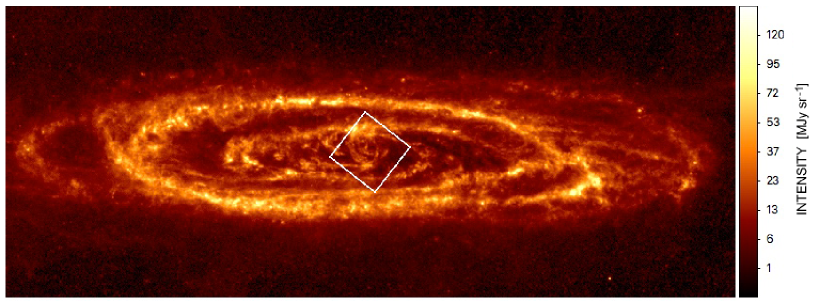
Figure 1: M31 as viewed in the 250 $\mu$m band by the Herschel SPIRE instrument. The square box delineates the “ZoomZone” discussed in the text. Its size is 700 arcsec on a side, corresponding to 2.65 kpc based on an assumed distance of 780 kpc.

2 Methodology

In contrast with previous approaches to the dust mapping problem, the ppmap procedure drops the assumptions of uniform dust temperature and opacity index along the line of sight (Marsh et al., 2015). After taking proper account of the point-spread function and spectral response of the telescope, it returns a pair of four-dimensional hypercubes containing, respectively, the expectation values of differential column density,

$$N_{{}_{T\beta}} \equiv \frac{\partial^{2}\!N}{\partial T_{{}_{\rm D}}\,\partial\beta_{{}_{\rm D}}}\,,$$

and their associated uncertainties, as a function of $(x,y,T_{{}_{\rm D}},\beta_{{}_{\rm D}})$. Here $\beta_{{}_{\rm D}}$ is the opacity index of the dust in the far-infrared i.e.

$$\beta_{{}_{\rm D}} = -\,\frac{d\log\kappa_{\lambda}}{d\log\lambda}\,;$$ (2.1)

$\kappa_{\lambda}$ is the mass opacity coefficient of the dust at wavelength $\lambda$, and the derivative is evaluated in the wavelength interval covered by Herschel. Thus $N_{{}_{T\beta}}(x,y,T_{{}_{\rm D}},\beta_{{}_{\rm D}})$ is the best estimate of the line-of-sight column density at $(x,y)$, in unit dust temperature interval about $T_{{}_{\rm D}}$ and unit opacity index interval about $\beta_{{}_{\rm D}}$. The procedure assumes only that the emitting dust is in radiative equilibrium, and that, at the observed wavelengths, the emission is optically thin. It works by defining a grid of discrete values of $x$, $y$, $T_{{}_{\rm D}}$ and $\beta_{{}_{\rm D}}$, which represent sampling locations in the continuous state space of $(x,y,T_{{}_{\rm D}},\beta_{{}_{\rm D}})$. It then iterates towards the set of differential column densities, in the vicinities of those grid points, that best reproduces the observed monochromatic intensities. The resolution on the plane of the sky $(x,y)$ is increased by a factor of about 4.5 relative to the standard analysis procedure, yielding maps of angular resolution of $\sim 8^{\prime\prime}$, sampled by $4^{\prime\prime}$ square pixels

The dust temperature sampling interval is arbitrary. For this work, we have used twelve representative dust temperatures that are equally spaced in logarithm between $\,10.0\,{\rm K}\,$ and $\,50.0\,{\rm K}$, i.e. $T_{1}\!=\!10.0\,{\rm K}$, $T_{2}\!=\!11.6\,{\rm K}$, $T_{3}\!=\!13.4\,{\rm K}$, $T_{4}\!=\!15.5\,{\rm K}$, $T_{5}\!=\!18.0\,{\rm K}$, $T_{6}\!=\!20.8\,{\rm K}$, $T_{7}\!=\!24.1\,{\rm K}$, $T_{8}\!=\!27.8\,{\rm K}$, $T_{9}\!=\!32.2\,{\rm K}$, $T_{10}\!=\!37.3\,{\rm K}$, $T_{11}\!=\!43.2\,{\rm K}\,$ and $T_{12}\!=\!50.0\,{\rm K}$.

The opacity index sampling interval is also arbitrary, and we have used four representative values equally spaced linearly between $\,\beta_{{}_{\rm D}}\!=\!1.5\,$ and $\,\beta_{{}_{\rm D}}\!=\!3.0\,$, i.e. $\,\beta_{1}\!=\!1.5$, $\,\beta_{2}\!=\!2.0$, $\,\beta_{3}\!=\!2.5\,$ and $\,\beta_{4}\!=\!3.0$. If we were to invoke more representative dust temperatures and/or opacity indices, the computational cost of the analysis would increase proportionately but further accuracy would not necessarily be gained.

Our column density scale is based on an assumed opacity of 0.1 cm² g^-1 at a wavelength of 300 $\mu$m. The reference opacity is defined with respect to total mass (dust plus gas). Although observationally determined it is consistent with a gas to dust ratio of 100 (Hildebrand, 1983), and we use it here on the assumption that interstellar dust grains in M31 have similar properties to those in our own Galaxy.

Given the $\,N_{{}_{T\beta}}\,$ hypercube, we can integrate out $\beta$ to obtain two three-dimensional data-cubes containing, respectively, representative values of

$$N_{{}_{T}} \equiv \frac{dN}{dT_{{}_{\rm D}}}\;\,=\;\,\int\limits_{{\rm all}\;\beta_{{}_{\rm D}}}\;\frac{\partial^{2}\!N}{\partial T_{{}_{\rm D}}\,\partial\beta_{{}_{\rm D}}}\;d\beta_{{}_{\rm D}}$$ (2.2)

and their associated uncertainties. $\,N_{{}_{T}}(x,y,T_{{}_{\rm D}})\,$ is the best estimate of column density along the line of sight at $(x,y)$, in unit dust temperature interval about $\,\sim\!T_{{}_{\rm D}}$. This data cube can be interpreted in two interesting ways. First, we can take slices at the different representative dust temperatures, $T_{i}$, and plot separately the column density of dust in each dust temperature interval, $((T_{i-1}T_{i})^{1/2}\leq T_{{}_{\rm D}}\leq(T_{i}T_{i+1})^{1/2})$. Second, we can consider individual pixels separately, and analyse the mass-weighted distribution of dust temperature along the line of sight through the pixel. Since the dust temperature depends on the ambient radiant energy density, $U_{{}_{\rm RAD}}$ (in relatively unshielded regions, $T_{{}_{\rm D}}\propto U_{{}_{\rm RAD}}^{0.20\pm 0.05}$), this can help to resolve regions along the line of sight that have different ambient radiation fields.

Similarly, we can integrate out $T_{{}_{\rm D}}$ to obtain two three-dimensional data-cubes containing, respectively, representative values of

$$N_{{}_{\beta}} \equiv \frac{dN}{d\beta_{{}_{\rm D}}}\;\,=\;\,\int\limits_{{\rm all}\;T_{{}_{\rm D}}}\;\frac{\partial^{2}\!N}{\partial T_{{}_{\rm D}}\,\partial\beta_{{}_{\rm D}}}\;dT_{{}_{\rm D}}$$ (2.3)

and their associated uncertainties. $\,N_{{}_{\beta}}(x,y,\beta_{{}_{\rm D}})\,$ is the best estimate of the line-of-sight column density at $(x,y)$, in unit opacity index interval about $\,\sim\!\beta_{{}_{\rm D}}$. Again, this data cube can be interpreted in two interesting ways. First, we can take slices at the different representative opacity indices, $\beta_{j}$, and plot the column density of dust in each opacity index interval, $(\beta_{j}-0.25\leq\beta_{{}_{\rm D}}\leq\beta_{j}+0.25)$. Second, we can consider individual pixels separately, and analyse the mass-weighted distribution of opacity index along the line of sight through the pixel. Since the opacity index depends on the constitution of the dust (size, composition, shape), this can help to distinguish regions along the line of sight that have different chemical histories.

Next, we can integrate out both $\beta_{{}_{\rm D}}$ and $T_{{}_{\rm D}}$, to obtain two two-dimensional maps of

$$N = \int\limits_{{\rm all}\;T_{{}_{\rm D}}}\;\frac{dN}{dT_{{}_{\rm D}}}\;dT_{{}_{\rm D}}$$ (2.4)

and its associated uncertainty. Here $N(x,y)$ gives the best estimate for the line-of-sight column density at $(x,y)$.

We can obtain an estimate of the mass-weighted mean dust temperature, ${\bar{T}}_{{}_{\rm D}}(x,y)$, along the line of sight at $(x,y)$,

$${\bar{T}}_{{}_{\rm D}} = \frac{1}{N}\,\int\limits_{{\rm all}\;T_{{}_{\rm D}}}\;T_{{}_{\rm D}}\;\frac{dN}{dT_{{}_{\rm D}}}\;dT_{{}_{\rm D}}\,,$$ (2.5)

and higher-order moments of the dust temperature distribution along the line of sight (standard deviation, skewness and kurtosis), as discussed below.

Finally, we can obtain an estimate of the mass-weighted mean opacity index, ${\bar{\beta}}_{{}_{\rm D}}(x,y)$, along the line of sight at $(x,y)$ using an integral analogous to Eq. (2.5).

3 Observations

M31 was observed using the Herschel PACS and SPIRE instruments which provided continuum images in bands centred on wavelengths of 70, 100, 160, 250, 350, and 500 $\mu$m. Full details of the observing strategy, calibration, and map-making procedures are given by Fritz et al. (2012) and Smith et al. (2012). As an example, Fig.1 shows a SPIRE image of M31 in the 250 $\mu$m band.

The spatial resolution values of the scan maps, i.e., the beam sizes at full width half maximum (FWHM), are approximately 8.5, 12.5, 13.3, 18.2, 24.5, and 36.0 arcsec at the six wavelengths, respectively. For our analysis we use PSFs based on the measured Herschel beam profiles (Poglitsch et al., 2010; Griffin et al., 2013).

4 Results

The above data have been used to generate a 4D hypercube of differential column density as a function of sky location, dust temperature, and dust opacity index, from which we can derive various line-of-sight integrated quantities such as the integrated column density of dust plus gas, $N$, the mean dust temperature, ${\bar{T}_{{}_{\rm D}}}$, and the mean dust opacity index ${\bar{\beta}}_{{}_{\rm D}}$. Here, and in the following discussion, an overscore (e.g. ${\bar{T}}_{{}_{\rm D}}$ and ${\bar{\beta}}_{{}_{\rm D}}$) denotes mass-weighted averages along the line of sight.

Fig. 2 shows the radial variation of azimuthally averaged values of these quantities, $<\!\!\!N\!\!\!>$, $<\!\!\!{\bar{T}}_{{}_{\rm D}}\!\!\!>$, and $<\!\!{\bar{\beta}}_{{}_{\rm D}}\!\!>$, at each galactocentric radius. Galactocentric radii are estimated assuming that the midplane of Andromeda makes an angle of $\theta=77^{\rm o}$ with the plane of the sky, and that the position angle of the tilt axis is $38^{\circ}$. We note that the radial plot of $<\!\!{\bar{\beta}}_{{}_{\rm D}}\!\!>$ in this figure indicates a central dip in the dust opacity index, consistent with previous reports by Smith et al. (2012) and Draine et al. (2014). In particular there is detailed correspondence with Fig. 13 of Draine et al. (2014), including the local maximum at $r\sim 3$ kpc.

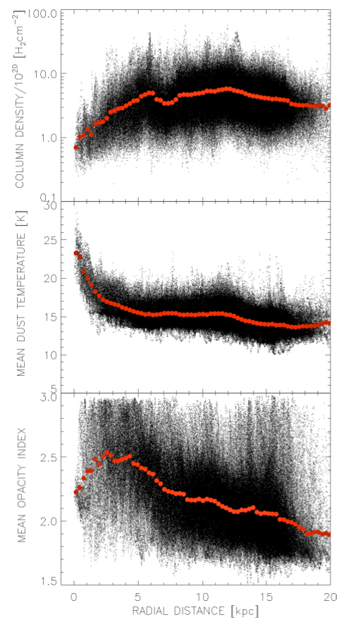
Figure 2: Radial variation of total line-of-sight column density, $<\!\!\!N\!\!\!>$, mean dust temperature, $<\!\!\!{\bar{T}}_{{}_{\rm D}}\!\!\!>$, and mean dust opacity index, $<\!\!{\bar{\beta}}_{{}_{\rm D}}\!\!>$. The red filled circles represent averages in 300 pc bins.

4.1 The central region: “ZoomZone”

In the remainder of the paper, we focus on the small region of Andromeda that is marked with a square of width 700 arcsec (2.65 kpc) on Fig. 1, and refer to it as the ZoomZone. It is chosen because it includes the circumnuclear environment, the site of some interesting physical processes which are not well understood (see, for example Li, Wang & Wakker, 2009). Fig. 3 shows maps of temperature-differential column density, $N_{T}$, in this region, at all 12 temperatures. These maps, and the associated uncertainty maps, are available in the on-line material as described in Appendix B.

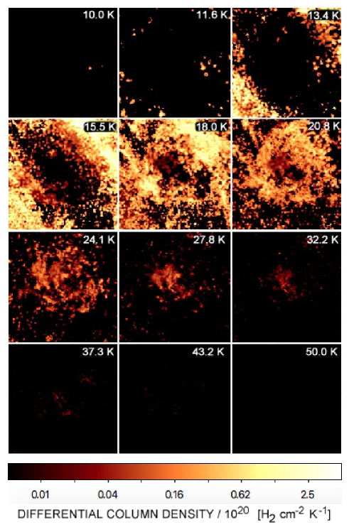
Figure 3: Maps of differential column density as a function of temperature, for the ZoomZone. These maps have been truncated at the $5\sigma$ level. The field of view in each case is 700 arcsec (2.65 kpc) square.

On the first (top) row of Fig. 4 are maps of (a) ${\hat{N}}$, (b) ${\hat{T}}_{{}_{\rm D}}$ and (c) ${\hat{\beta}}_{{}_{\rm D}}$ obtained by Smith et al. (2012) using the standard analysis procedure, cropped at the boundaries of the ZoomZone. The second (middle) row shows the corresponding maps obtained with ppmap, viz. (d) the integrated column density, $N$, (e) the mass-weighted mean dust temperature, ${\bar{T}}_{{}_{\rm D}}$, and (f) the mass-weighted mean opacity index, ${\bar{\beta}}_{{}_{\rm D}}$. These maps illustrate the greatly increased resolution obtained with ppmap. In addition, they demonstrate the ability of ppmap to dig out large quantities of cold dust that is underestimated by the standard analysis procedure. This is illustrated by the presence of lower mean dust temperatures (by up to 2 K) in panel (e) than panel (b), while Fig. 3 shows the presence of significantly cooler dust ($\sim 10$ K as opposed to $\sim 15$ K) than indicated by the standard analysis in the corresponding region. As a consequence, in many areas ppmap obtains a lower mean dust temperature (${\bar{T}}_{{}_{\rm D}}<{\hat{T}}_{{}_{\rm D}}$), and a higher net column density ($N>{\hat{N}}$). The third (bottom) row shows (g) the relative standard deviation, $\sigma_{T}/\bar{T}_{\rm D}$, (h) the skewness, Skew$(T)$, and (i) the kurtosis, Kurt$(T)$ of the dust temperature distribution along each line of sight. These three quantities are defined by:

$$\sigma_{T}\! = \!\left(\frac{1}{N}\!\int\limits_{{\rm all}\;T_{{}_{\rm D}}}\frac{dN}{dT_{{}_{\rm D}}}(T_{{}_{\rm D}}-{\bar{T}}_{{}_{\rm D}})^{2}\,\,dT_{{}_{\rm D}}\right)^{1/2}$$ (4.1)

$${\rm Skew}(T)\! = \!\left(\frac{1}{N}\!\int\limits_{{\rm all}\;T_{{}_{\rm D}}}\frac{dN}{dT_{{}_{\rm D}}}(T_{{}_{\rm D}}-{\bar{T}}_{{}_{\rm D}})^{3}\,\,dT_{{}_{\rm D}}\right)/\sigma_{T}^{3}$$ (4.2)

$${\rm Kurt}(T)\! = \!\left(\frac{1}{N}\!\int\limits_{{\rm all}\;T_{{}_{\rm D}}}\frac{dN}{dT_{{}_{\rm D}}}(T_{{}_{\rm D}}-{\bar{T}}_{{}_{\rm D}})^{4}\,\,dT_{{}_{\rm D}}\right)/\sigma_{T}^{4}$$ (4.3)

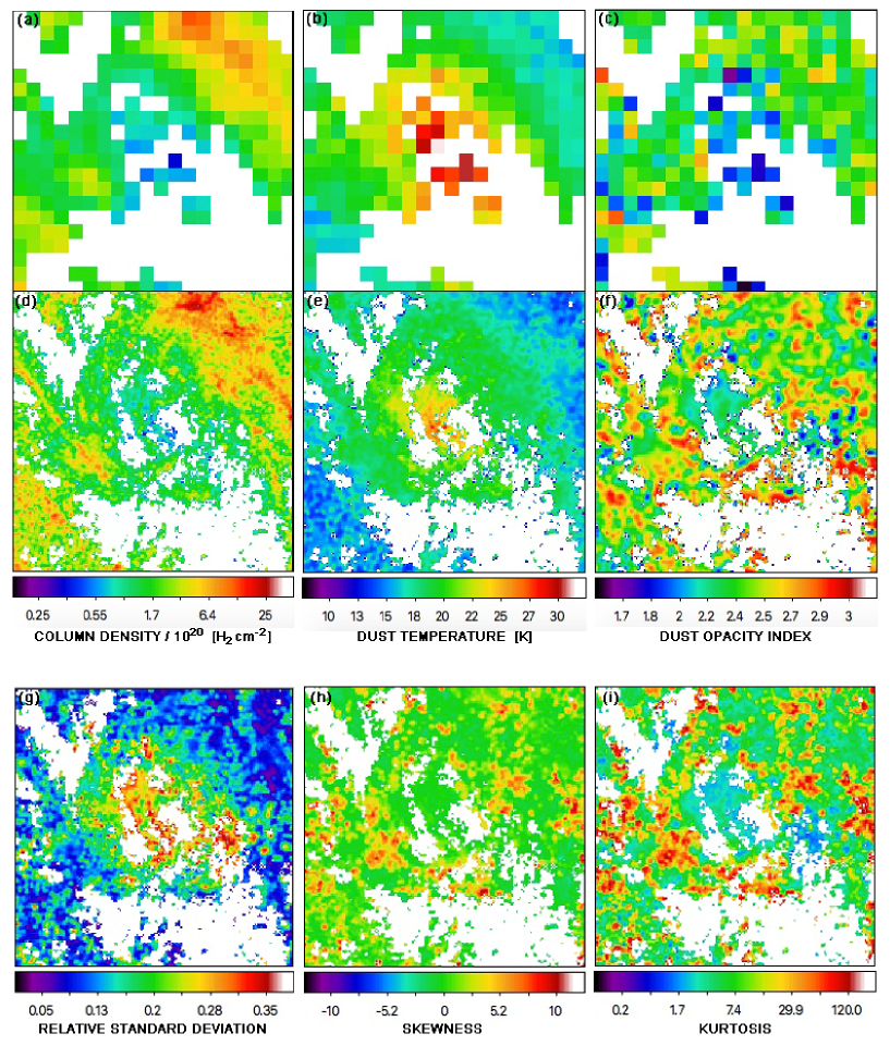
Figure 4: Maps of line-of-sight integrated quantities for the ZoomZone, each with a field of view of 700 arcsec (2.65 kpc) square, and each truncated at the $5\sigma$ level with respect to column density. Top row: Maps obtained by Smith et al. (2012) using the standard analysis procedure, viz. (a) Integrated column density, ${\hat{N}}$, (b) mean dust temperature, ${\hat{T}}_{{}_{\rm D}}$ and (c) mean dust opacity index, ${\hat{\beta}}_{{}_{\rm D}}$. Middle row: The corresponding maps obtained with ppmap, viz. (d) the integrated column density, $N$, (e) the mass-weighted mean dust temperature, ${\bar{T}}_{{}_{\rm D}}$, and (f) the mass-weighted mean opacity index, ${\bar{\beta}}_{{}_{\rm D}}$. Bottom row: Maps of the higher order moments of the dust temperature distribution, viz. (g) the standard deviation, $\sigma_{T}$, expressed as a fraction of the local mean temperature, ${\bar{T}}_{{}_{\rm D}}$, (h) the skewness, and (i) the kurtosis.

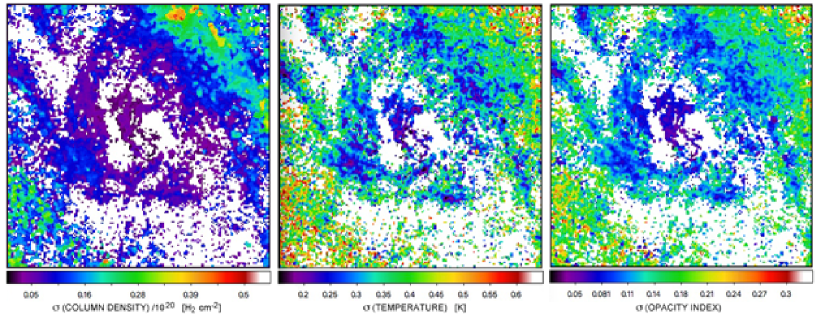
Figure 5: Uncertainty maps of column density, temperature, and opacity index for the ZoomZone, each with a field of view of 700 arcsec (2.65 kpc) square. They represent the uncertainty values corresonding to the maps in the middle row of Fig. 4.

They provide information on the form of the temperature distribution along each line of sight. In particular, for a pure Gaussian distribution we would expect a skewness of zero and a kurtosis of 3. Examination of Fig. 4 shows that these conditions are met over much of the ZoomZone, although there are localised regions in which the kurtosis is large ($\stackrel{{\scriptstyle>}}{{{}_{\sim}}}100$ in many cases). Large values of the kurtosis indicate the presence of a significant number of high-temperature outliers in the tail of the distribution. It is not clear what high-kurtosis implies physically; comparison with published positions of planetary nebulae (Merrett et al., 2006), X-ray sources (Stiele et al., 2011), and supernova remnants (Lee & Lee, 2014) indicate little or no correspondence with high-kurtosis features in the ZoomZone, while none of the HII regions listed by Azimlu et al. (2011) falls within that zone. However, comparison over the full field of M31 shows a high degree of correlation with the locations of HII regions from the Azimlu et al. (2011) survey, in the sense that HII regions are preferentially located in regions of high temperature kurtosis and, interestingly, low standard deviation of temperature. This suggests that high kurtosis might be a signpost of star formation, and this is confirmed by comparison with a map of star formation rate (Ford et al., 2014). It would clearly be interesting to investigate what kurtosis and the other temperature moments tell us about star formation, but since the current focus is on the nuclear region, we defer a discussion of more global phenomena to a future paper.

The uncertainty maps corresponding to the middle row of Fig. 4 (column density, temperature, and opacity index) are presented in Fig. 5.

Fig. 6 shows a set of scatter plots, for the ZoomZone, between all pairs of the six quantities, i.e., column density, temperature, opacity index, and temperature standard deviation, skewness and kurtosis. Various correlations are apparent, including an anticorrelation between kurtosis and standard deviation which, as mentioned above, appears to be a global characteristic. Also, particularly relevant here are the correlations involving the nuclear bar-like feature, plotted in red. This feature clearly shows some systematic behaviour, one example being that the dust opacity index, ${\bar{\beta}}_{{}_{\rm D}}(x,y)$, is positively correlated with dust temperature in the interior of the nuclear spiral (within 270 pc of the nucleus). This goes against the larger-scale trend in which ${\bar{\beta}}_{{}_{\rm D}}(x,y)$, is anticorrelated with $\bar{T}_{{}_{\rm D}}$ within the central $\sim 3$ kpc. As discussed by Smith et al. (2012), various explanations are possible for that anticorrelation, such as the destruction of grain ice-mantles in the increasingly intense interstellar radiation field towards the centre of the galaxy. However, the fact that it switches to a positive correlation near the very centre would seem to argue against that explanation, although it might instead indicate that a separate population of grains is present.

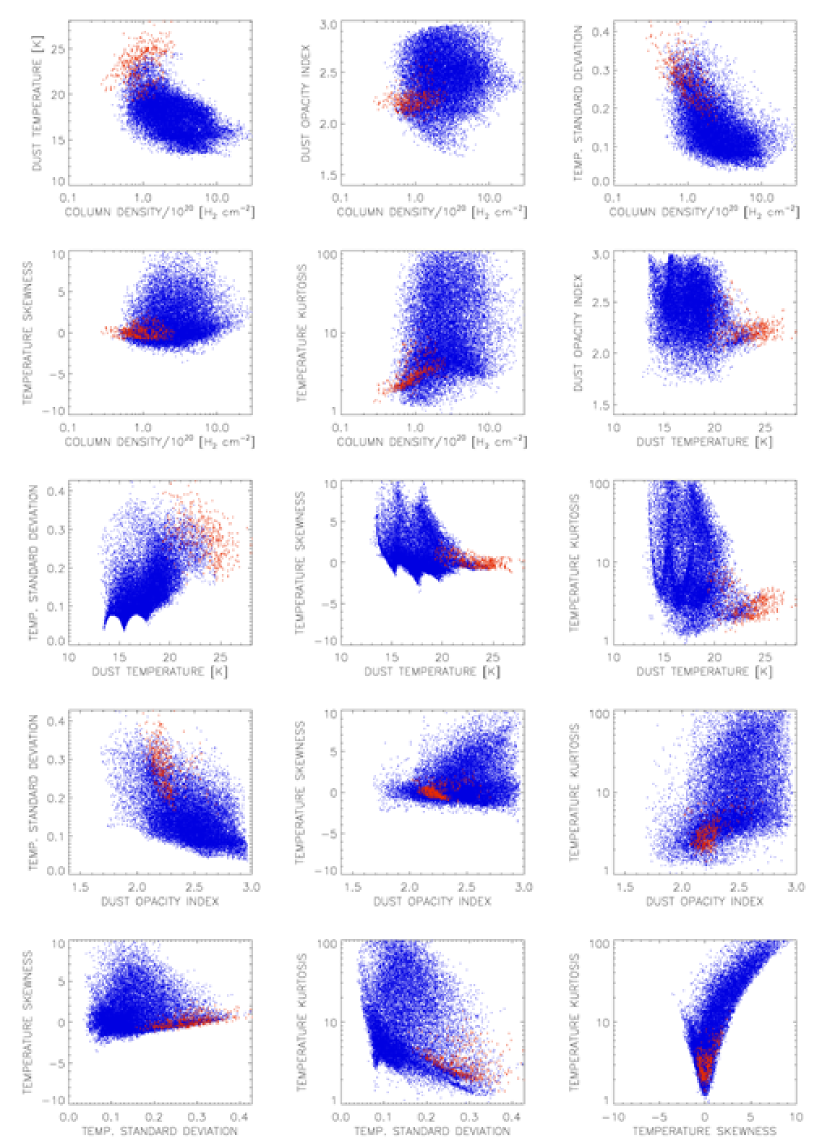
Figure 6: Scatter plots of line-of-sight integrated quantities for the ZoomZone. The standard deviation of temperature is expressed as a fraction of the local mean line-of-sight temperature. The red points represent spatial locations within the central bar-like feature in the nuclear spiral, within 270 pc of the nucleus. The spiky lower envelopes in the plots of $\sigma_{T}$ and Skew$(T)$ versus $T_{{}_{\rm D}}$ are due to the discretisation of temperature values in ppmap.

Fig. 7 represents a three-temperature composite for the ZoomZone. It shows that the innermost portion is dominated by a bar-like feature which appears to consist of a pair of hot, roughly parallel, strands with a central crossover. It is distinctly visible at other wavelengths, such as H$\alpha$ (Jacoby, Ford & Ciardullo, 1985) and 70 $\mu$m (in our Herschel image), although less so at 24 $\mu$m (Gordon et al., 2006) due to confusion by a dense concentration of bulge stars. Its nature has been the subject of debate, but with a length of only $\sim 500$ pc, it clearly does not correspond to the much larger ($\sim 10$ kpc) bar inferred from near-infrared morphology and dynamical simulations (Athanassoula & Beaton, 2006).

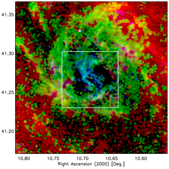
Figure 7: Three-temperature composite of the ZoomZone, where the dust temperature ranges correspond to the colours indicated. The white square delineates the inner portion corresponding to the field of view of the extinction map of Dong et al. (2016).

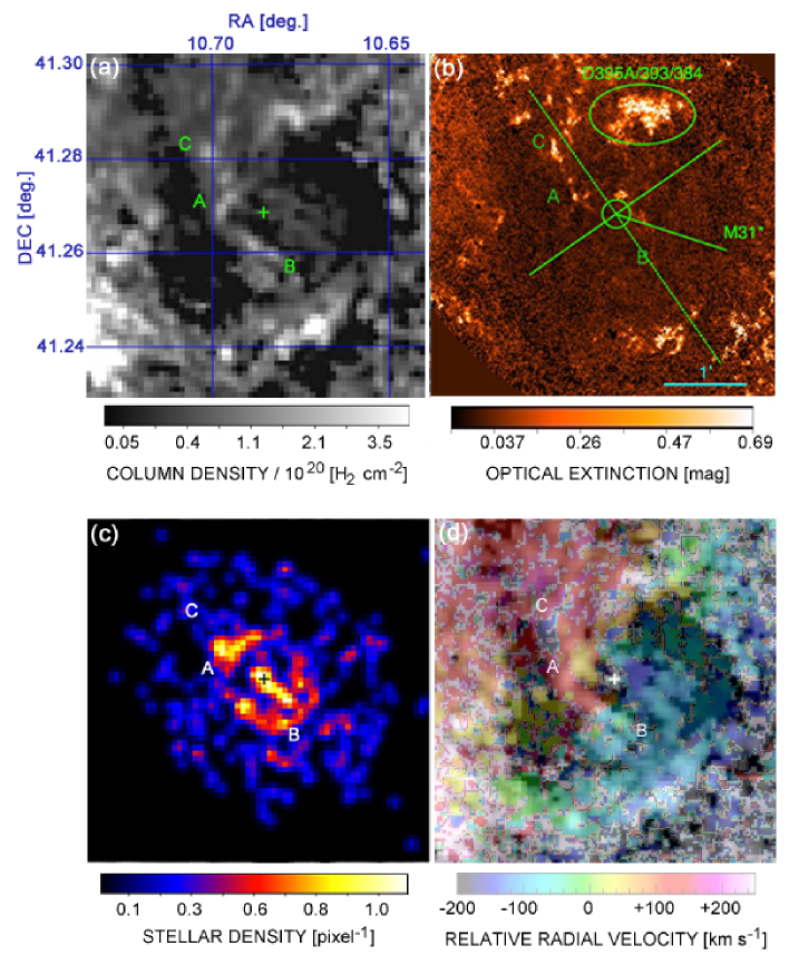
Figure 8: Comparison of column density, extinction, stellar density, and radial velocity distributions for the central bulge region of M31, as delineated by the white square in Fig. 7. (a) Total column density; (b) Optical extinction at a wavelength of 5447 Å, from Dong et al. (2016); (c) Stellar density in units of stars per pixel, representing the number density of 2MASS sources with $J\leq 14$, smoothed by a Gaussian kernel of FWHM = 2 pixels (8 arcsec); (d) Radial velocity with respect to the systemic value of 300 km s^-1, superposed on the total column density distribution. The radial velocities are from [NII] observations published previously by Boulesteix et al. (1987). In panels (a), (c), and (d), the position of the nucleus is marked by a plus sign (+). In (b) it is labelled as M31*. “A”, “B”, and “C” are reference points discussed in the text.

4.2 The nature of the bar-like feature

Some information on the 3D geometry of the bar-like feature can be obtained from a comparison of the column density distribution derived here on the basis of dust emission, and a previously published extinction map (Dong et al., 2016), as shown in panels (a) and (b) of Fig. 8. These maps show some distinct differences. For example the filamentary structure which extends between reference points “A” and “B” in the column density map is absent in the extinction map, suggesting that it lies behind the bulge and hence behind the source of illumination which enables foreground features to be detected in extinction. This behaviour was also noted by Dong et al. (2016) who identify the feature with a dusty clump detected in CO and conclude, similarly, that it is located on the far side of the bulge. We will thus refer to the feature in question as the “rear filament”. However, an adjacent filament which extends from the nucleus (“+”) to point “C” is seen prominently in both emission and absorption, indicating that it is closer to us. This segment is part of a longer filament which passes directly over the nucleus in line-of-sight projection. We refer to this filament as the “central filament”. Based on its elevated dust temperature (see Fig. 4e), it likely passes directly through the centre of the bulge where the interstellar radiation field due to evolved giant stars is strongest. Its overall position angle is $\sim 50^{\circ}$, although it contains a central “jog” whereby it runs approximately east-west over the nucleus.

If the central filament is the manifestation of a bar, representing orbital motion under the influence of a bar-like gravitational potential (see, for example Sellwood & Wilkinson, 1993), we would expect to see some evidence of it in the distribution of bulge stars. Panel (c) of Fig. 8 shows that this is indeed the case—the bar structure is clearly visible in a map of stellar density. The latter represents the number density of 2MASS sources brighter than $14^{\rm th}$ magnitude at $J$ band, estimated using a circular Gaussian kernel whose width (FWHM) corresponds to 2 pixels (8 arcsec). The position angle of the stellar bar is approximately $45^{\circ}$, reasonably consistent with that of the central filament. We thus interpret the central dust structure as a bar, and explain its apparently double appearance in the column density map as a line-of-sight juxtaposition with the “rear filament” which is actually located further back.

Further elucidation of the nature of the central structure can be obtained from a comparison with radial velocity information. Since the morphology of the dust distribution closely resembles that of the ionized gas (Li, Wang & Wakker, 2009), we make use of radial velocities of [NII], published previously by Boulesteix et al. (1987). Such a comparison is facilitated by panel (d) of Fig. 8, which represents a superposition of the [NII] radial velocities on the dust column density distribution. The general trend of the radial velocities (red-shifted at the upper left and blue-shifted at the lower right) is consistent with the general rotational motion in the kinematic model presented by Melchior & Combes (2011), involving an inner disk tilted at a position angle of $70^{\circ}$ and an inclination of $43^{\circ}$ to the plane of the sky. For the reasons discussed above, we now believe that this disk is actually a compact spiral containing a classical bar.

Fig. 8(d) also shows that the profile of radial velocity along the central filament is quite distinct from that of the general rotational motion. It changes abruptly from a red-shift to a blue-shift as the nucleus position is traversed, at which point the velocity gradient is approximately east-west, consistent with the local orientation of the jog in the filament. This velocity structure, together with the apparent positional coincidence between the central filament and nucleus, would indicate motion either towards or away from the nucleus. However, we can eliminate the latter possibility because of the orientation—the lower right portion of the filament must be pointed away from us since it experiences more optical extinction then the upper left portion. Such an orientation is, in fact, consistent with the inferred tilt of the nuclear spiral as a whole, based on the Melchior & Combes (2011) kinematic model. We thus conclude that the red- and blue-shifts indicate motion towards the nucleus, i.e., that the filament constitutes an accretion channel. Since the filament appears to connect with the nuclear spiral at diametrically opposite points, it seems likely that these spiral arms provide the source of the inflow.

We can estimate the inflow rate given the column density of the central filament ($\sim 2\times 10^{20}$ H₂ masses per cm²), the radial velocity $\sim 100$ km s^-1, the inclination ($\sim 47^{\circ}$ to the line of sight) and an estimated width of 8 arcsec (60 pc). We thereby obtain a total flow rate (from both sides) of $\sim 0.05$ $M_{\odot}$ yr^-1. This value greatly exceeds, by 8 orders of magnitude, the minimum accretion rate (based on mass-energy equivalence) required to power the central X-ray source, the estimated luminosity of which is $\simeq 1.2\times 10^{36}$ erg s^-1 (Li, Wang & Wakker, 2009). It is also exceeds, by 3 orders of magnitude, the Bondi accretion rate estimated by Li et al. It is, however, close to the inflow rate required for continuous replenishment of the hot corona according to the evaporation model of Li et al.

The role of the bar as a conduit for gas flow inwards from the spiral arms to the nucleus in barred galaxies has been established observationally (Knapen, Pérez-Ramírez & Laine, 2002) and has been the subject of a number of theoretical and modelling studies in which the inflow is attributed to bar-induced torques (see, for example, García-Burillo et al., 2009; Querejeta et al., 2015; Hopkins & Quataert, 2011). It is not uncommon for nesting of bars to occur, whereby a subkiloparsec (secondary) nuclear bar exists within a large-scale primary bar (Laine et al., 2002; Shlosman & Heller, 2002; Wozniak, 2015). We suggest that M31 represents an example of such nesting. Future dynamical modelling will be needed to determine whether our inferred nuclear bar can supply sufficient torque to drive the suggested inflow, and to establish the dynamical relationship between the primary and secondary bars.

Appendix A Extension of ppmap to enable $\beta$ estimation

The original version of ppmap (Marsh et al., 2015) treated the opacity index, $\beta_{{}_{\rm D}}$, as constant. We have extended the algorithm by treating $\beta_{{}_{\rm D}}$ as an additional state variable, thus enabling the generation of 4D hypercubes of differential column density as a function of RA, Dec, $T_{{}_{\rm D}}$, and $\beta_{{}_{\rm D}}$. In doing so it is necessary to guard against the well-known degeneracy between $T_{{}_{\rm D}}$ and $\beta_{{}_{\rm D}}$, whereby the presence of measurement noise induces an anticorrelation between the estimates of those quantities. Various approaches have been proposed for dealing with this problem, most of which are oriented towards fitting the observed spectral energy distributions (SEDs) of models of multiple uniform clumps in a given field. In the Hierarchical Bayesian approach (Kelly et al., 2012; Galliano, 2018) the solution is constrained by the use of a prior distribution designed to represent the statistics of the source population as a whole and whose parameters are estimated adaptively from the observations. The algorithm then works towards finding solutions which minimize the dispersion of the estimated parameter values, and appears to work well provided one can characterise the source population by a single mode. However, extending the hierarchical Bayesian scheme to the more general imaging problem would present difficulties since it would belong in the category of single-pixel SED fitting techniques requiring all input images to be smoothed to the same resolution, thus losing an important advantage of ppmap. In addition, one would need to assume a single temperature and opacity index along each line of sight and this, in itself, leads to difficulties in deducing dust properties (Juvela et al., 2013). The ppmap procedure is not subject to that restriction.

We can, however, achieve the main goal of suppressing the $T_{{}_{\rm D}}$-$\beta_{{}_{\rm D}}$ degeneracy using a non-hierarchical Bayesian scheme in which we specify a priori the population statistics regarding $\beta_{{}_{\rm D}}$. For this purpose we assume that the a priori probability distribution of possible $\beta_{{}_{\rm D}}$ values is described by a Gaussian function characterised by mean and standard deviation ${\bar{\beta}}$ and $\sigma_{\beta}$, respectively. The estimation procedure is then essentially the same as described in Marsh et al. (2015), except as noted below. As before, the desired differential column density, represented by vector $\rho$, is obtained numerically by a stepwise integration of the differential equation:

$$\frac{\partial\rho}{\partial t}+\phi_{1}\rho=0\,,$$ (A.1)

where $\phi_{1}$ is the conditioning factor which contains information on both the measurement model and the data, and $t$ is a progress variable which increases from 0 to 1 during the solution procedure. The only modification necessary for incorporating the prior information regarding $\beta_{{}_{\rm D}}$ is that the initial condition, $\rho_{(t=0)}=\eta$ is now replaced with:

$${\rho_{n}}(t=0)=\eta\times\alpha\exp[-(\beta_{n}-{\bar{\beta}})^{2}/(2\sigma_{\beta}^{2})]$$ (A.2)

in which the index $n$ refers to the $n$th cell in the state space for which the local value of $\beta_{{}_{\rm D}}$ is equal to $\beta_{n}$, and $\alpha$ is a normalisation constant designed to ensure that the average value of $\rho_{n}(t=0)$ over all $n$ is equal to $\eta$. The latter quantity represents the a priori dilution, as defined by Marsh et al. (2015), for which we have assumed a value of 0.3 in our M31 analysis.

For the Gaussian prior on $\beta_{{}_{\rm D}}$ we have assumed ${\bar{\beta}}$ = 2.0 and $\sigma_{\beta}$ = 0.35. In regions where the signal to noise ratio is high, these parameters have essentially no effect on the solution, so that no bias results (see, for example, Galliano, 2018), and this is true of both the hierarchical and non-hierarchical Bayesian approaches. However, in regions of low signal to noise, the algorithm will default to the prior itself so that, in essence, we are taking $\beta_{{}_{\rm D}}$ to be 2.0 except where the data compel us otherwise.

Appendix B Supplementary material

We have made available online the set of ppmap output files for M31. They consist of a set of files in FITS format which include:

1. 4D hypercube of differential column density, with axes RA, Dec, dust temperature ($T_{{}_{\rm D}}$), and dust opacity index ($\beta_{{}_{\rm D}}$). The sets of grid values of $T_{{}_{\rm D}}$ and $\beta_{{}_{\rm D}}$ are specified in the FITS header.

2. 4D hypercube of $1\sigma$ uncertainty values of differential column density

3. 2D map of integrated line-of-sight column density in units of $10^{20}$ H₂ molecules cm^-2, truncated at the $5\sigma$ level.

4. 2D map of mean line-of-sight dust opacity index, truncated at the $5\sigma$ level.

5. 2D map of mean line-of-sight dust temperature, truncated at the $5\sigma$ column density level.

6. 2D map of the standard deviation of dust temperature along the line of sight, truncated at the $5\sigma$ column density level.

7. 2D map of the skewness of the dust temperature distribution along the line of sight, truncated at the $5\sigma$ column density level.

8. 2D map of the kurtosis of the dust temperature distribution along the line of sight, truncated at the $5\sigma$ column density level.

References

- Athanassoula & Beaton (2006) Athanassoula, E. & Beaton, R. L. 2006, MNRAS, 370, 1499
- Azimlu et al. (2011) Azimlu, M., Marciniak, R., & Barmby, P. 2011, ApJ, 142, 139
- Beaton et al. (2007) Beaton, R. L., Majewski, S. R., Guhathakurta, P. et al. 2007, ApJ, 658, L91
- Block et al. (2006) Block, D. L., Bournaud, F., Combes, F. et al. 2006, Nature, 443, 832
- Boulesteix et al. (1987) Boulesteix, J., Georgelin, Y. P., Lecoarer, E., Marcelin, M. & Monnet, G. 1987, A&A 178, 91
- Ciardullo et al. (1988) Ciardullo, R., Rubin, V. C., Jacoby, G. H. et al. 1988, AJ, 95, 438
- Diaz et al. (2017) Diaz, M. B., Wegg, C., Gerhard, O. 2017, MNRAS, 466, 4279
- Dong et al. (2016) Dong, H., Li, Z., Wang, Q. D. et al. 2016, MNRAS, 459, 2262
- Draine et al. (2014) Draine, B. T., Aniano, G., Krause, O. et al. 2014, ApJ, 780, 172
- Ford et al. (2014) Ford, G. P., Gear, W. K., Smith, M. W. L. et al. 2013, ApJ, 769, 55
- Fritz et al. (2012) Fritz, J., Gentile, G., Smith, M. W. L. et al. 2012, A&A, 546, 34
- Galliano (2018) Galliano, F. 2018, MNRAS, 476, 1445
- García-Burillo et al. (2009) García-Burillo, S., Fernández-García, S., Combes, F. et al. 2009 A&A, 496, 85
- Gordon et al. (2006) Gordon, K. D., Bailin, J., Engelbracht, C. W. et al. 2006, ApJ, 638, L87
- Griffin et al. (2013) Griffin, M. J., North, C. E., Amaral-Rogers, A. et al. 2013, MNRAS, 434, 992
- Groves et al. (2012) Groves, B., Krause, O., Sandstrom, K. et al. 2012, MNRAS, 426, 892
- Habing et al. (1984) Habing, H. J., Miley, G., Young, E. et al. 1984, ApJ, 278, L59
- Hildebrand (1983) Hildebrand, R. H. 1983, QJRAS, 24, 267
- Hopkins & Quataert (2011) Hopkins, P. F. & Quataert, E. 2011, MNRAS, 415, 1027
- Jacoby, Ford & Ciardullo (1985) Jacoby, G. H., Ford, H. & Ciardullo, R. 1985, ApJ, 290, 136
- Juvela et al. (2013) Juvela, M., Montillaud, J., Ysard, N., Lunttila, T. 2013, A&A, 556, A63
- Kelly et al. (2012) Kelly, B. C., Shetty, R., Stutz, A. M. et al. 2012, ApJ, 752, 55
- Kirk et al. (2015) Kirk, J. M., Gear, W. K., Fritz, J. et al. 2015, ApJ, 798, 58
- Knapen, Pérez-Ramírez & Laine (2002) Knapen, J. H., Pérez-Ramírez & Laine, S. 2002, MNRAS, 337, 808
- Laine et al. (2002) Laine, S., Shlosman, I., Knapen, J. H., & Peletier, R. F. 2002, ApJ, 567, 97
- Lee & Lee (2014) Lee, J. H. & Lee, M. G. 2014, ApJ, 786, 130
- Lewis et al. (2015) Lewis, A. R., Dolphin, A. E., Dalcanton, J. J. et al. 2015, ApJ, 805, 183
- Li, Wang & Wakker (2009) Li, Z., Wang, Q. D. & Wakker, B. P. 2009, 397, 148
- Marsh et al. (2015) Marsh, K. A., Whitworth, A. P. & Lomax, O., 2015, MNRAS, 454, 4282
- Melchior & Combes (2011) Melchior, A.-L. & Combes, F. 2011, A&A, 536, A52
- Melchior & Combes (2013) Melchior, A.-L. & Combes, F. 2013, A&A, 549, A27
- Merrett et al. (2006) Merrett, H. R., Merrifield, M. R., Douglas, N. G. et al. 2006, MNRAS, 369, 120
- Opitsch (2016) Opitsch, M. 2016, The bar of the Andromeda galaxy revealed by integral field spectroscopy. Ludwig-Maximilians-Universität München, Germany
- Pilbratt et al. (2010) Pilbratt, G. L., Riedinger, J. R., Passvogel, T., et al. 2010, A&A, 518, L1
- Poglitsch et al. (2010) Poglitsch, A., Waelkens, C., Geis, N., et al. 2010, A&A, 518, L2
- Querejeta et al. (2015) Querejeta, M., Meidt, S. E., Schinnerer, E. et al. 2016, A&A, 588, 33
- Sellwood & Wilkinson (1993) Sellwood, J. A. & Wilkinson, A. 1993, Rep. Prog. Phys., 56, 173
- Shlosman & Heller (2002) Shlosman, I. & Heller, C. H. 2002, ApJ, 565, 921
- Smith et al. (2012) Smith, M. W. L., Eales, S. A., Gomez, H. L. et al. 2012, ApJ, 756, 40
- Stanek & Garnavich (1998) Stanek, K. Z. & Garnavich, P. M. 1998, ApJ, 503, L131
- Stiele et al. (2011) Stiele, H., Pietsch, W., Haberl, F. et al. 2011, A&A, 534, A55
- Vilardell et al. (2006) Villardell, F., Ribas, I., & Jordi, C. 2006, A&A, 459, 321
- Wozniak (2015) Wozniak, H. 2015, A&A, 575, A7