Unpolarized isovector quark distribution function from Lattice QCD:
A systematic analysis of renormalization and matching

Abstract

We present a detailed Lattice QCD study of the unpolarized isovector quark Parton Distribution Function (PDF) using large-momentum effective theory framework. We choose a quasi-PDF defined by a spatial correlator which is free from mixing with other operators of the same dimension. In the lattice simulation, we use a Gaussian-momentum-smeared source at $M_{\pi}=356$ MeV and $P_{z}\in\{1.8,2.3\}$ GeV. To control the systematics associated with the excited states, we explore five different source-sink separations. The nonperturbative renormalization is conducted in a regularization-independent momentum subtraction scheme, and the matching between the renormalized quasi-PDF and $\overline{\rm MS}$ PDF is calculated based on perturbative QCD up to one-loop order. Systematic errors due to renormalization and perturbative matching are also analyzed in detail. Our results for lightcone PDF are in reasonable agreement with the latest phenomenological analysis.

I Introduction

Parton distribution functions (PDFs) of nucleons are not only important quantities characterizing the internal hadron structures but are also key ingredients to make predictions for high-energy scattering processes Butterworth:2015oua ; Alekhin:2017kpj ; Gao:2017yyd . Thus calculating PDFs from first principles has been a holy grail in nuclear and particle physics. Since PDFs are embedded with the low-energy quark and gluon degrees of freedom in the hadron, they involve infrared (IR) dynamics of strong interactions and can only be determined by nonperturbative methods such as Lattice QCD.

Within QCD factorization Collins:2011zzd , the quark PDF is defined as

$$q(x,\mu)\equiv\!\int\!{d\xi^{-}\over 4\pi}e^{-ixP^{+}\xi^{-}}\!\langle P|\bar{\psi}(\xi^{-})\gamma^{+}U(\xi^{-},0)\psi(0)|P\rangle,$$ (1)

where $|P\rangle$ denotes the nucleon state with momentum $P_{\mu}=(P_{t},0,0,P_{z})$. $x$ is the quark momentum fraction, $\mu$ is the renormalization scale in the $\overline{\rm MS}$ scheme. $\xi^{\pm}=(t\pm z)/\sqrt{2}$ are the lightcone coordinates. The light-like Wilson line is introduced to maintain the gauge invariance:

$$U(\xi^{-},0)=P\exp\biggl{(}-ig\int_{0}^{\xi^{-}}d\eta^{-}A^{+}(\eta^{-})\biggr{)}\ .$$ (2)

PDFs are defined with lightcone coordinates, but the Lattice simulation can only be conducted in Euclidean space with no proper treatment for lightcone quantities which involves real time. Thus simulating PDFs on a Euclidean Lattice is an extremely difficult task. Early studies based on operator product expansion (OPE) were only able to derive the lowest few moments of the PDFs Martinelli:1987zd ; Martinelli:1988xs ; Detmold:2001dv ; Dolgov:2002zm .

Recently, a novel approach that allows to directly access the $x$-dependence of PDFs from Lattice QCD was proposed in Ref. Ji:2013dva , now formulated as large-momentum effective theory (LaMET) Ji:2014gla . Within this framework, one can extract PDFs—as well as other lightcone quantities—from the correlations of certain static operators in a nucleon state. On the one hand, the static correlations, often referred to as quasi observables, can be directly calculated on a Euclidean Lattice and depend dynamically on the nucleon momentum. On the other hand, at large momentum, the quasi observables can be factorized into the parton observable and a perturbative matching coefficient, up to corrections suppressed by powers of the large nucleon momentum. Equating the results from the two sides provides a straightforward way to determine the lightcone PDFs.

To calculate the quark PDF in LaMET, one starts with a “quasi-PDF” which is defined as an equal-time correlation of quarks along the $z$ direction Ji:2013dva :

$$\widetilde{q}_{\Gamma}(x,P_{z})\equiv\int_{-\infty}^{\infty}{dz\over 4\pi}e^{ixP_{z}z}\langle P|O_{\Gamma}(z)|P\rangle\,.$$ (3)

In the above, $O_{\Gamma}(z)=\bar{\psi}(z)\Gamma U(z,0)\psi(0)$ with $\Gamma=\gamma^{z}$ or $\Gamma=\gamma^{t}$, and the space-like Wilson line is:

$$U(z,0)=P\exp\left(-ig\int_{0}^{z}dz^{\prime}A_{z}(z^{\prime})\right).$$ (4)

For finite but large momentum $P_{z}$, $\widetilde{q}(x,P_{z})$ has support in $-\infty<x<\infty$. Unlike the lightcone PDF that is boost invariant, the quasi-PDF has a nontrivial dependence on the nucleon momentum $P_{z}$. After renormalizing the quasi-PDF in a scheme such as the regularization-independent momentum subtraction (RI/MOM) scheme, one can match the renormalized quasi-PDF to the $\overline{\rm MS}$ PDF through the factorization theorem Ji:2013dva ; Ji:2014gla ; Stewart:2017tvs ; Izubuchi:2018srq ; Ma:2014jla ; Ma:2017pxb :

$$\widetilde{q}(x,P_{z},p^{R}_{z},\mu_{R})= \int_{-1}^{1}{dy\over|y|}\>C\left({x\over y},r,\frac{yP_{z}}{\mu},\frac{yP_{z}}{p_{z}^{R}}\right)\,q(y,\mu)$$

$$+\mathcal{O}\left({M^{2}\over P_{z}^{2}},{\Lambda_{\text{QCD}}^{2}\over x^{2}P_{z}^{2}}\right),$$ (5)

where $p_{z}^{R}$ and $\mu_{R}$ are introduced in RI/MOM scheme: $p_{z}^{R}$ is the momentum of the involved parton and $\mu_{R}$ is renormalization scale. $r=\mu_{R}^{2}/(p_{z}^{R})^{2}$, $C$ is the perturbative matching coefficient, and $\mathcal{O}(M^{2}/P_{z}^{2},\Lambda_{\rm QCD}^{2}/x^{2}P_{z}^{2})$ denotes nucleon mass and higher-twist contributions suppressed by powers of the large nucleon momentum. The flavor indices in $q,\ \widetilde{q}$ and $C$ are implied. When $-1<y<0$, the distributions refer to the antiquark distributions.

Since the proposal of LaMET, remarkable progress has been made in both theoretical aspect and Lattice calculations. It should be pointed out that these developments are achieved in an interactive way. The LaMET was first used to calculate the proton isovector quark distribution $f_{u-d}$ Lin:2014zya ; Alexandrou:2015rja ; Chen:2016utp ; Alexandrou:2016jqi ; Chen:2018fwa ; Alexandrou:2018eet , including the unpolarized, polarized and transversity cases, and subsequently to the meson distribution amplitudes Zhang:2017bzy ; Chen:2017gck . The first Lattice studies used the matching coefficients at one-loop order in a transverse-momentum cutoff scheme Xiong:2013bka ; Ji:2015qla ; Xiong:2015nua . However, as was found in Ref. Xiong:2013bka , the original quasi-PDF suffers from an ultraviolet (UV) linear divergence which might pose a severe problem for the renormalization of its Lattice matrix elements Li:2016amo ; Rossi:2017muf ; Rossi:2018zkn . Then many attentions have been paid to the renormalization property Ji:2015jwa ; Ishikawa:2016znu ; Chen:2016fxx ; Xiong:2017jtn ; Constantinou:2017sej ; Ji:2017oey ; Ishikawa:2017faj ; Green:2017xeu ; Spanoudes:2018zya , and finally the multiplicative renormalizability of quasi-PDF in coordinate space in the continuum was proven to all orders in strong coupling constant $\alpha_{s}$ Ji:2017oey ; Ishikawa:2017faj . This finding has further motivated the Lattice analysis of nonperturbative renormalization (NPR) of the quasi-PDF Alexandrou:2017huk ; Chen:2017mzz ; Green:2017xeu in the RI/MOM scheme Martinelli:1994ty , and the calculation of the matching coefficients between the RI/MOM quasi-PDFs and $\overline{\rm MS}$ PDFs Stewart:2017tvs . Besides the renormalization, the finite nucleon mass corrections were also worked out to all orders of $M^{2}/P_{z}^{2}$ Chen:2016utp , and higher-twist $\mathcal{O}(\Lambda^{2}_{\rm QCD}/x^{2}P_{z}^{2})$ effects were numerically removed by extrapolating the results at several $P_{z}$ values to infinite momentum Lin:2014zya ; Chen:2016utp . Based on these studies, calculations of the isovector quark PDF at physical pion mass have become available Lin:2017ani ; Alexandrou:2018pbm ; Chen:2018xof ; Alexandrou:2018eet . Potential operator mixing in the Lattice renormalization of the quasi-PDF has also been investigated Constantinou:2017sej ; Alexandrou:2017huk ; Green:2017xeu ; Chen:2017mzz , and the mixing pattern classified in Ref. Chen:2017mie . Ways to reduce the systematic uncertainties from Fourier transforming the spatial correlation at long distance were proposed in Refs. Lin:2017ani ; Chen:2017lnm . The LaMET was also attempted to study transverse-momentum-dependent distributions Ji:2014hxa ; Ji:2018hvs ; Ebert:2018gzl ; Ebert:2019okf ; Ebert:2019tvc ; Ji:2019sxk ; Shanahan:2019zcq ; Ji:2019ewn , as well as the gluon PDF Wang:2017qyg ; Wang:2017eel ; Fan:2018dxu ; Zhang:2018diq ; Li:2018tpe ; Wang:2019tgg .

In addition to LaMET, other interesting approaches have been proposed in recent years to calculate the PDFs from Lattice QCD. For example, one can extract the PDFs from a class of “Lattice cross sections” Ma:2014jla ; Ma:2017pxb , while a smeared quasi-PDF in the gradient flow method was proposed to sweep the power divergence in the Lattice calculation Monahan:2016bvm ; Monahan:2017hpu . One can also study a pseudo distribution Radyushkin:2017cyf , related to the quasi-PDF through Fourier transforms. While this method shows interesting renormalization features Orginos:2017kos ; Karpie:2017bzm , it coincides with LaMET regarding the factorization into PDFs Ji:2017rah ; Zhang:2018ggy ; Izubuchi:2018srq . Moreover there are proposals using current-current correlators to compute the hadronic tensor Liu:1993cv ; Liang:2017mye , or the higher moments of the PDF, lightcone distribution amplitudes, etc. Detmold:2005gg ; Braun:2007wv ; Liang:2017mye ; Chambers:2017dov ; Bali:2018spj ; Bali:2019ecy . These different approaches are subject to their own systematics, but they can be compared to each other.

It was argued that the power divergent mixing between local moment operators may spoil the renormalization of quasi-PDFs Rossi:2017muf ; Rossi:2018zkn , however such problem dissolves in LaMET since one first needs to take the continuum limit of the quasi-PDF after renormalization on the Lattice, and then match it to obtain the $x$-dependence of the PDF. The factorization has been derived rigorously Ma:2014jla ; Izubuchi:2018srq in the continuum, and one only needs to focus on the renormalization of the nonlocal spatial correlator only. Thus the renormalization of local moment operators is irrelevant to quasi-PDF. Besides, there are also confusions on the LaMET matching between Minkowskian and Euclidean matrix elements of the quasi-PDF Carlson:2017gpk , which have been clarified in Refs. Ji:2017rah ; Briceno:2017cpo .

Most of the available Lattice calculations have used $\Gamma=\gamma^{z}$ (except Chen:2018xof ; Alexandrou:2018pbm ) for the unpolarized quasi-PDF, which is now known to mix with the scalar quasi-PDF operator $O_{I}$ at $O(a^{0})$ Constantinou:2017sej ; Chen:2017mie ; Green:2017xeu . This operator mixing introduces an additional systematic uncertainty in nonperturbative renormalization Alexandrou:2017huk ; Chen:2017mzz ; Green:2017xeu ; Lin:2017ani , thus limiting the accuracy of the extracted PDF. On the contrary, the $\Gamma=\gamma^{t}$ case is free from operator mixing with $O_{I}$ at $O(a^{0})$ Constantinou:2017sej ; Chen:2017mie ; Green:2017xeu . Therefore, it is highly desirable to start from the quasi-PDF with $\Gamma=\gamma^{t}$. This is one main motif of this study.

In this work, we will carry out a Lattice calculation of the unpolarized isovector quark distribution from the quasi-PDF with $\Gamma=\gamma^{t}$ with the same nonperturbative renormalization procedure as for the $\Gamma=\gamma^{z}$ case in Ref. Chen:2017mzz . The calculation is performed using clover fermions on a CLS ensemble of gauge configurations with $N_{f}=2+1$ (degenerate up/down, and strange) flavors under open boundary condition Luscher:2011kk with pion mass $M_{\pi}=356$ MeV and Lattice spacing $a=0.086$ fm Bruno:2014jqa . We will examine the dependence on the nucleon momentum $P_{z}$ and the RI/MOM scales $p_{z}^{R}$, $\mu_{R}$, as well as on choices of the projection operator for the amputated Green’s function in RI/MOM renormalization. Due to large uncertainties, it is hard to see the sea quark asymmetry observed in early studies which were performed without Lattice renormalization Lin:2014zya ; Alexandrou:2015rja ; Chen:2016utp ; Alexandrou:2016jqi . In the future we plan to analyze CLS ensembles with a better accuracy and down to physical masses and $a<0.04$ fm, both for $(m_{s}+m_{u}+m_{d})$ fixed to its physical value and for physical $m_{s}$ using flavour SU(3) and SU(2) extrapolations.

The rest of this paper is organized as follows. In Sec. II, we briefly review the procedure of nonperturbative renormalization and matching of the quasi-PDF in the RI/MOM scheme, in particular the explicit one-loop matching coefficient for the $\Gamma=\gamma^{t}$ case. In Sec. III, we describe the details of Lattice simulation of the hadronic matrix elements as well as its nonperturbative renormalization. Systematic errors in the calculation are also discussed in this section. In Sec. IV, we present our results on the $x$-dependence of the unpolarized isovector quark PDF with the statistical and systematic uncertainties, and the last section contains the summary of our work.

II Nonperturbative Renormalization and Matching

To recover the continuum limit of a quasi-PDF matrix element, nonperturbative renormalization on the Lattice is required to deal with linear and logarithmic UV divergences. In this work, we follow the RI/MOM scheme elaborated in Refs. Stewart:2017tvs ; Chen:2017mzz , and match the result to the $\overline{\rm MS}$ PDF with the one-loop matching coefficient Stewart:2017tvs .

II.1 RI/MOM renormalization on the Lattice

The spatial correlator $O_{\Gamma}(z)$ has been proven to be multiplicatively renormalizable in coordinate space in the continuum Ji:2017oey ; Ishikawa:2017faj , which enables the renormalization in RI/MOM scheme Martinelli:1994ty .

For each value of $z$, the RI/MOM renormalization factor $Z$ is obtained by requiring loop corrections for the matrix element of a quasi-PDF operator vanish in an off-shell quark state at a given momentum:

$$Z(z,p^{R}_{z},a^{-1},\mu_{R})=\left.\frac{\sum_{s}\langle p,s|O_{\gamma^{t}}(z)|p,s\rangle}{\sum_{s}\langle p,s|O_{\gamma^{t}}(z)|p,s\rangle_{\rm tree}}\right|_{\tiny\begin{matrix}p^{2}=-\mu_{R}^{2}\\ \!\!\!\!p_{z}=p^{R}_{z}\end{matrix}}\,.$$ (6)

The bare matrix element $\sum_{s}\langle p,s|O_{\gamma^{t}}(z)|p,s\rangle$ will be calculated on the Lattice from the amputated Green’s function $\Lambda_{\gamma^{t}}(p,z)$ of $O_{\gamma^{t}}(z)$, with a projection operator ${\cal P}$ for the Dirac matrix:

$$\sum_{s}\langle p,s|O_{\gamma^{t}}(z)|p,s\rangle=\mbox{Tr}\left[\Lambda_{\gamma^{t}}(z,p){\cal P}\right]\,.$$ (7)

Due to the breaking of Lorentz covariance in $O_{\Gamma}(z)$, the RI/MOM subtraction depends on two scales $\mu_{R}$ and $p_{z}^{R}$. As a result, the renormalization factor $Z(z,p^{R}_{z},a^{-1},\mu_{R})$ depends on the Lattice spacing as well as on the two RI/MOM scales $\mu_{R}$ and $p^{R}_{z}$.

Based on the symmetry of $O_{\Gamma}(z)$ on the Lattice, the amputated Green’s function $\Lambda_{\gamma^{t}}(p,z)$ is not only proportional to the tree-level result $\gamma^{t}$, but also includes two other independent Lorentz structures:

$$\Lambda_{\gamma^{t}}(p,z)=\widetilde{F}_{t}(p,z)\gamma^{t}+\widetilde{F}_{z}(p,z)\frac{p_{t}\gamma^{z}}{p_{z}}+\widetilde{F}_{p}(p,z)\frac{p_{t}\not{p}}{p^{2}}\,.$$ (8)

In the above $\widetilde{F}_{i}$s are independent form factors that are invariant under the hyper cubic group $H(4)$. According to Eq. (8) the RI/MOM renormalization factor $Z$ will also depend on the projection operator ${\cal P}$. One can choose to single out $\widetilde{F}_{t}$ only Stewart:2017tvs , which we call the minimal projection. This projection has the simplest form but captures all the UV divergence in $\Lambda_{\gamma^{t}}(p,z)$. Optionally, one can choose ${\cal P}=\not{p}/(4p^{t})$, which we call the $\not{p}$ projection. The renormalization factors $Z$ with the minimal and $\not{p}$ projections are defined as:

$$Z_{mp}(z,p^{R}_{z},a^{-1},\mu_{R})\equiv\widetilde{F}_{t}(p,z)\Big{|}_{\tiny\begin{matrix}p^{2}=-\mu_{R}^{2}\\ \!\!\!\!p_{z}=p^{R}_{z}\end{matrix}},$$ (9)

$$Z_{\not{p}}(z,p^{R}_{z},a^{-1},\mu_{R})$$

$$\equiv\Big{[}\widetilde{F}_{t}(p,z)+\widetilde{F}_{z}(p,z)+\widetilde{F}_{p}(p,z)\Big{]}\bigg{|}_{\tiny\begin{matrix}p^{2}=-\mu_{R}^{2}\\ \!\!\!\!p_{z}=p^{R}_{z}\end{matrix}}.$$ (10)

The bare nucleon matrix element from a Lattice calculation in coordinate space

$$\widetilde{h}(z,P_{z},a^{-1})={1\over 2P^{0}}\langle P|O_{\gamma^{t}}(z)|P\rangle$$

is renormalized according to

$$\widetilde{h}_{R}(z,P_{z},p^{R}_{z},\mu_{R})$$

$$=\left.Z^{-1}(z,p^{R}_{z},a^{-1},\mu_{\tiny R})\widetilde{h}(z,P_{z},a^{-1})\right|_{a\to 0}.$$ (11)

Here $\widetilde{h}_{R}(z,P_{z},p^{R}_{z},\mu_{R})$ is the continuum limit of the renormalized matrix element. Consequently, the quasi-PDF $\widetilde{q}_{R}(x,P_{z},p^{R}_{z},\mu_{R})$ in RI/MOM scheme is obtained through the Fourier transformation of $\widetilde{h}_{R}(z,P_{z},p^{R}_{z},\mu_{\tiny R})$:

$$\widetilde{q}_{R}(x,P_{z},p^{R}_{z},\mu_{R})=P_{z}\int{dz\over 2\pi}\ e^{ixP_{z}z}\widetilde{h}_{R}(z,P_{z},p^{R}_{z},\mu_{R}).$$

In RI/MOM, $\widetilde{h}_{R}(z,P_{z},p^{R}_{z},\mu_{R})$ and $\widetilde{q}_{R}(x,P_{z},p^{R}_{z},\mu_{R})$ are independent of the UV regulator, and the one-step matching between the quasi-PDF and $\overline{\rm MS}$ PDF can be carried out in the continuum theory with dimensional regularization Stewart:2017tvs .

The quasi-PDFs will eventually be matched to the same $\overline{\text{MS}}$ PDF, and the two projections with $Z_{mp}$ and $Z_{\not{p}}$ should generate the same result. However the matching coefficient can only be calculated at a fixed loop order, hence remanent dependence on the projection operator is inevitable.

Using the same logic one reaches the conclusion that the quasi-PDF’s dependence on the RI/MOM scales $\mu_{R}$ and $p_{z}^{R}$ should also be fully cancelled by the matching coefficient. Any fixed-order matching calculation will inevitably lead to a residual $\mu_{R}$, $p_{z}^{R}$, and $P_{z}$ dependence of the final result for the PDF. These dependencies should be carefully studied and included in the systematic uncertainties.

II.2 One-loop matching for quasi-PDF and PDF

To obtain the matching coefficient between the quasi-PDF $\widetilde{q}_{R}(x,P_{z},p^{R}_{z},\mu_{R})$ and lightcone PDF $q(x,\mu)$, one can calculate the off-shell quark matrix elements in perturbation theory. In the following, the calculation will be conducted in Landau gauge for both minimal and $\not{p}$ projections. See Appendix .1 for the results in a general covariant gauge with a general Lorentz structure.

The lowest order quark quasi-PDF is

$$\widetilde{q}^{(0)}(x)=\delta(1-x)\,.$$ (13)

At one-loop order, it is

$$\widetilde{q}^{(1)}(x,p,\rho)=\mbox{Tr}\left[\left(\left[\widetilde{f}_{t}(x,\rho)\right]_{+}\gamma^{t}+\left[\widetilde{f}_{z}(x,\rho)\right]_{+}\frac{p_{t}}{p_{z}}\gamma^{z}+\left[\widetilde{f}_{p}(x,\rho)\right]_{+}\frac{p_{t}\not{p}}{p^{2}}\right){\cal P}\right]\,.$$ (14)

The $\widetilde{f}_{i}$s are

$$\widetilde{f}_{t}(x,\rho)=\frac{\alpha_{s}C_{F}}{2\pi}\left\{\begin{array}[]{lc}\frac{8x^{2}(1-x)-x\rho(13-10x)+3\rho^{2}}{2(1-x)(1-\rho)(4x-4x^{2}-\rho)}+\frac{4x(2-x)-x\rho-3\rho}{4(1-x)(1-\rho)^{3/2}}\ln\frac{2x-1+\sqrt{1-\rho}}{2x-1-\sqrt{1-\rho}}&x>1\\ \frac{x(-7+4x)+3\rho}{2(1-x)(1-\rho)}+\frac{4x(2-x)-\rho(3+x)}{4(1-x)(1-\rho)^{3/2}}\ln\frac{1+\sqrt{1-\rho}}{1-\sqrt{1-\rho}}&0<x<1\\ -\frac{8x^{2}(1-x)-x\rho(13-10x)+3\rho^{2}}{2(1-x)(1-\rho)(4x-4x^{2}-\rho)}-\frac{4x(2-x)-x\rho-3\rho}{4(1-x)(1-\rho)^{3/2}}\ln\frac{2x-1+\sqrt{1-\rho}}{2x-1-\sqrt{1-\rho}}&x<0\end{array}\right.,$$ (18)

$$\widetilde{f}_{z}(x,\rho)=\frac{\alpha_{s}C_{F}}{2\pi}\left\{\begin{array}[]{lc}\begin{array}[]{l}\frac{-32x^{2}(1-x)^{2}(2x-1)-4x\rho(8-43x+65x^{2}-38x^{3}+8x^{4})+\rho^{2}(5-41x+42x^{2}-8x^{3})+2\rho^{3}(2-x)}{2(1-x)(1-\rho)^{2}(4x-4x^{2}-\rho)^{2}}\\ \quad+\frac{4-8x+8x^{2}+\rho(3-13x+4x^{2})+2\rho^{2}}{4(1-x)(1-\rho)^{5/2}}\ln\frac{2x-1+\sqrt{1-\rho}}{2x-1-\sqrt{1-\rho}}\end{array}&x>1\\ \frac{-5+15x-12x^{2}-2\rho(2-3x)}{2(1-x)(1-\rho)^{2}}+\frac{4-8x+8x^{2}+\rho(3-13x+4x^{2})+2\rho^{2}}{4(1-x)(1-\rho)^{5/2}}\ln\frac{1+\sqrt{1-\rho}}{1-\sqrt{1-\rho}}&0<x<1\\ \begin{array}[]{l}-\frac{-32x^{2}(1-x)^{2}(2x-1)-4x\rho(8-43x+65x^{2}-38x^{3}+8x^{4})+\rho^{2}(5-41x+42x^{2}-8x^{3})+2\rho^{3}(2-x)}{2(1-x)(1-\rho)^{2}(4x-4x^{2}-\rho)^{2}}\\ \quad-\frac{4-8x+8x^{2}+\rho(3-13x+4x^{2})+2\rho^{2}}{4(1-x)(1-\rho)^{5/2}}\ln\frac{2x-1+\sqrt{1-\rho}}{2x-1-\sqrt{1-\rho}}\end{array}&x<0\end{array}\right.,$$ (26)

$$\widetilde{f}_{p}(x,\rho)=\frac{\alpha_{s}C_{F}}{2\pi}\left\{\begin{array}[]{lc}\frac{16x\rho(1-x)^{2}(1-6x)-2\rho^{2}(1-22x+26x^{2}-4x^{3})-\rho^{3}(7-6x)}{2(1-\rho)^{2}(4x-4x^{2}-\rho)^{2}}+\frac{-\rho(8-12x+\rho)}{4(1-\rho)^{5/2}}\ln\frac{2x-1+\sqrt{1-\rho}}{2x-1-\sqrt{1-\rho}}&x>1\\ \frac{2-4x+\rho(7-8x)}{2(1-\rho)^{2}}+\frac{-\rho(8-12x+\rho)}{4(1-\rho)^{5/2}}\ln\frac{1+\sqrt{1-\rho}}{1-\sqrt{1-\rho}}&0<x<1\\ -\frac{16x\rho(1-x)^{2}(1-6x)-2\rho^{2}(1-22x+26x^{2}-4x^{3})-\rho^{3}(7-6x)}{2(1-\rho)^{2}(4x-4x^{2}-\rho)^{2}}-\frac{-\rho(8-12x+\rho)}{4(1-\rho)^{5/2}}\ln\frac{2x-1+\sqrt{1-\rho}}{2x-1-\sqrt{1-\rho}}&x<0\end{array}\right.,$$ (30)

and

$$\rho=\frac{-p^{2}-i\epsilon}{p_{z}^{2}}$$ (31)

with $i\epsilon$ giving the prescription to analytically extrapolate $\rho$ from $\rho<1$ (Minkowski) to $\rho>1$ (Euclidean). Notice that the vector current conservation guarantees that vertex corrections and wave function contributions can be combined into generalized plus functions Stewart:2017tvs . These functions are defined with two arbitrary functions $h(x)$ and $g(x)$:

$$\int dx\left[{h(x)}\right]_{+}g(x) =\int dx\;h(x)\left[g(x)-g(1)\right]\,.$$ (32)

For the lightcone PDF with the same off-shell IR regulation in Landau gauge, the tree level contribution is

$$q^{(0)}(x)=\delta(1-x)\,,$$ (33)

and the one-loop correction in the $\overline{\text{MS}}$ scheme is

$$q^{(1)}(x,p,\mu)$$

$$= \mbox{Tr}\left[\left(\left[f_{+}\left(x,\frac{\mu^{2}}{p^{2}}\right)\right]_{+}\gamma^{+}+\left[f_{p}(x)\frac{p^{+}\not{p}}{p^{2}}\right]_{+}\right){\cal P}\right]\,.$$ (34)

Here

$$f_{+}\left(x,\frac{\mu^{2}}{p^{2}}\right)= \frac{\alpha_{s}C_{F}}{2\pi}\theta(x)\theta(1-x)\left[\frac{-5+10x-6x^{2}}{2(1-x)}\right.$$

$$\left.+\frac{1+x^{2}}{1-x}\ln\frac{\mu^{2}}{-x(1-x)p^{2}}\right]\,,$$ (35)

$$f_{p}(x)= \frac{\alpha_{s}C_{F}}{2\pi}(1-2x)\theta(x)\theta(1-x)\,.$$ (36)

To match the quasi-PDF to lightcone PDF, one needs to take the on shell limit ($p^{2}\to 0$ or $\rho\to 0$) and the large momentum limit ($p_{t}\to p_{z}$) for the bare quasi-PDF

$$\widetilde{q}^{(1)}_{B}(x,\rho)=\widetilde{q}^{(1)}(x,(p_{t}\to p_{z},\vec{p}_{\perp},p_{z}),\rho\to 0).$$ (37)

One can observe that both terms proportional to $\gamma^{t}$ and $\gamma^{z}$ in Eq. (14) approach lightcone operators in the large momentum limit and the combination of them captures the correct collinear behavior. Therefore the bare quasi-PDF in minimal projection is defined to pick up the coefficient of $\gamma^{t}$ and $\gamma^{z}$ in Eq. (14):

$$\widetilde{q}_{B}^{(1)}(x,\rho)\Big{|}_{mp}=\left[\widetilde{f}_{t}(x,\rho)+\widetilde{f}_{z}(x,\rho)\right]_{+}\bigg{|}_{\rho\to 0}\,.$$ (38)

For the lightcone PDF, the coefficient of $\gamma^{+}$ in Eq. (II.2) is used for minimal projection:

$$q^{(1)}(x,p,\mu)\Big{|}_{mp}=f_{+}\left(x,\frac{\mu^{2}}{p^{2}}\right)_{+}\,.$$ (39)

The bare matching coefficient is then derived as

$$f_{1,mp}\left(x,\frac{p_{z}}{\mu}\right)_{+}=\widetilde{q}^{(1)}_{B}(x,\rho)\Big{|}_{mp}-q^{(1)}(x,p,\mu)\bigg{|}_{mp},$$ (40)

where

$$f_{1,mp}\left(x,\frac{p_{z}}{\mu}\right)=\frac{\alpha_{s}C_{F}}{2\pi}$$

$$\times\left\{\begin{array}[]{lc}\displaystyle\frac{1+x^{2}}{1-x}\ln\frac{x}{x-1}+1&x>1\\ \displaystyle\frac{1+x^{2}}{1-x}\ln\frac{4x(1-x)p_{z}^{2}}{\mu^{2}}-\frac{x(1+x)}{1-x}&0<x<1\\ \displaystyle-\frac{1+x^{2}}{1-x}\ln\frac{x}{x-1}-1&x<0\end{array}\right..$$ (44)

In RI/MOM, the quasi-PDF is renormalized with an additional counterterm. We find that in the $|x|\to\infty$ limit , only $\widetilde{f}_{t}(x,\rho)$ behaves as $1/|x|$. When integrating over $x$, this term recovers UV divergence in the local limit $z=0$. Therefore, it is a natural choice to pick up the $\gamma^{t}$ term in Eq. (14) as a counterterm:

$$\widetilde{q}_{CT}^{(1)}\left(x,r,\frac{p_{z}}{p_{z}^{R}}\right)\bigg{|}_{mp} =\left[\left|\frac{p_{z}}{p_{z}^{R}}\right|f_{2,mp}\left(1+\frac{p_{z}}{p_{z}^{R}}(x-1),r\right)\right]_{+}\,.$$ (45)

Here $r=\mu_{R}^{2}/(p_{z}^{R})^{2}$, and

$$f_{2,mp}(x,r)=\widetilde{f}_{t}(x,r)=\frac{\alpha_{s}C_{F}}{2\pi}\left\{\begin{array}[]{lc}\frac{-3r^{2}+13rx-8x^{2}-10rx^{2}+8x^{3}}{2(r-1)(x-1)(r-4x+4x^{2})}+\frac{-3r+8x-rx-4x^{2}}{2(r-1)^{3/2}(x-1)}\tan^{-1}\frac{\sqrt{r-1}}{2x-1}&x>1\\ \frac{-3r+7x-4x^{2}}{2(r-1)(1-x)}+\frac{3r-8x+rx+4x^{2}}{2(r-1)^{3/2}(1-x)}\tan^{-1}\sqrt{r-1}&0<x<1\\ -\frac{-3r^{2}+13rx-8x^{2}-10rx^{2}+8x^{3}}{2(r-1)(x-1)(r-4x+4x^{2})}-\frac{-3r+8x-rx-4x^{2}}{2(r-1)^{3/2}(x-1)}\tan^{-1}\frac{\sqrt{r-1}}{2x-1}&x<0\end{array}\right..$$ (49)

Finally, the matching coefficient $C$ in the factorization formula given in Eq.(I) is derived as

$$C\left(x,r,\frac{p_{z}}{\mu},\frac{p_{z}}{p_{z}^{R}}\right) =\delta(1-x)+\left[\widetilde{q}^{(1)}_{B}(x,\rho)-q^{(1)}(x,p,\mu)-\widetilde{q}_{CT}^{(1)}\left(x,r,\frac{p_{z}}{p_{z}^{R}}\right)\right]\Bigg{|}_{mp}+{\cal O}(\alpha_{s}^{2})$$

$$=\delta(1-x)+\left[f_{1,mp}\left(x,\frac{p_{z}}{\mu}\right)-\left|\frac{p_{z}}{p_{z}^{R}}\right|f_{2,mp}\left(1+\frac{p_{z}}{p_{z}^{R}}(x-1),r\right)\right]_{+}+{\cal O}(\alpha_{s}^{2})\,.$$ (50)

Here the coupling $\alpha_{s}(\mu)$ is in the standard $\overline{\text{MS}}$ scheme. Note that the antiquark distribution is mapped into the region $-1<y<0$ by setting $q(y)=-\bar{q}(-y)$.

For $\not{p}$ projection, one has the bare quasi-PDF

$$\widetilde{q}_{B}^{(1)}(x,\rho)\Big{|}_{\not{p}}=\left[\widetilde{f}_{t}(x,\rho)+\widetilde{f}_{z}(x,\rho)+\widetilde{f}_{p}(x,\rho)\right]_{+}\,.$$ (51)

The lightcone PDF with a similar projection is

$$q^{(1)}(x,p,\mu)\Big{|}_{\not{p}}=\left[f_{+}\left(x,\frac{\mu^{2}}{p^{2}}\right)+f_{p}(x)\right]_{+}\,.$$ (52)

Under this projection, the matching coefficient for the bare quasi-PDF coincides with Eq. (40):

$$f_{1,\not{p}}\left(x,\frac{p_{z}}{\mu}\right)_{+} =\widetilde{q}^{(1)}_{B}(x,\rho)\Big{|}_{\not{p}}-q^{(1)}(x,p,\mu)\bigg{|}_{\not{p}}$$

$$=f_{1,mp}\left(x,\frac{p_{z}}{\mu}\right)_{+}\,.$$ (53)

The counter-term can be obtained by calculating with ${\cal P}=\not{p}/(4p^{t})$:

$$f_{2,\not{p}}(x,r)=\frac{\alpha_{s}C_{F}}{2\pi}\left\{\begin{array}[]{lc}\frac{3-3r-2x}{2(r-1)(x-1)}+\frac{4rx-8x^{2}+8x^{3}}{(r-4x+4x^{2})^{2}}+\frac{2-2r-rx+2x^{2}}{(r-1)^{3/2}(x-1)}\tan^{-1}\frac{\sqrt{r-1}}{2x-1}&x>1\\ \frac{3-3r-2x+4x^{2}}{2(r-1)(1-x)}+\frac{-2+2r+rx-2x^{2}}{(r-1)^{3/2}(1-x)}\tan^{-1}\sqrt{r-1}&0<x<1\\ -\frac{3-3r-2x}{2(r-1)(x-1)}-\frac{4rx-8x^{2}+8x^{3}}{(r-4x+4x^{2})^{2}}-\frac{2-2r-rx+2x^{2}}{(r-1)^{3/2}(x-1)}\tan^{-1}\frac{\sqrt{r-1}}{2x-1}&x<0\end{array}\right.\,.$$ (57)

The corresponding RI/MOM matching coefficient is obtained by replacing “$mp$” with “$\not{p}$” in Eq. (II.2), and the difference between $f_{2,\not{p}}$ and $f_{2,mp}$ vanishes in the $p_{z}^{R}$=0 limit. The matching coefficient with $\Gamma=\gamma^{z}$ is also given in Appendix .2.

III Lattice calculation of PDF

III.1 Lattice Matrix Elements

In this subsection, we give the results of a Lattice-QCD calculation using clover valence fermions on the CLS $32^{3}\times 96$ 2+1 flavor clover fermion ensemble H102 with Lattice spacing $a=0.086$ fm, pion mass $M_{\pi}=$ 356 MeV and box size $L\approx 2.7$ fm ($M_{\pi}L\approx 4.9$) Bruno:2014jqa . We use $\kappa_{l}=0.136865$ and $C_{SW}=1.98625$ for the valence clover fermion. We apply APE smearing Hasenfratz:2001hp with size=2.5$a$ twice in the source/sink smearing and also in the quasi-PDF operator $O_{\Gamma}$, but not in the fermion propagators.

Table 1: Momentum modes used in the NPR analysis. The four digits (in units of $2\pi/L$) in brackets correspond to three spatial momentum components and the energy component. The $z$ direction can be selected by setting the Wilson link along any of the three spatial directions. Thus these momentum modes approximately cover three choices of $\mu_{R}=\sqrt{-(p^{R})^{2}}$ and several sets of $p^{R}_{z}=2\pi i/L(i=0,1,2,...)$.

$a^{2}\mu_{R}^{2}$	Momentum modes $p^{R}$
$[1.109,1.118]$	(5,2,0,0) (4,3,1,5)
$[1.957,1.966]$	(5,5,0,3) (6,3,2,4) (5,4,1,9)
$[2.814,2.832]$	(6,5,1,10) (7,4,2,6) (6,3,0,16)

First of all, we will explore the nonperturbative renormalization in RI/MOM scheme. Following Ref. Chen:2017mzz , we use Landau gauge fixed wall sources (while limiting the source in the time slice range $t\in[32,64]$ to avoid the boundary effect from open boundary condition at $t$=0), and generate the propagators with the momentum modes listed in Table. 1. The four digits in brackets correspond to three spatial component and the energy component in units of $2\pi/L$. The $z$ direction can be selected by setting the Wilson link along any of the three spatial directions. Thus these results approximately cover three values of $\mu_{R}=\sqrt{-(p^{R})^{2}}$ (2.4, 3.2 and 3.9 GeV, corresponding to $a^{2}\mu_{R}^{2}$=1.1, 2.0 and 2.8), and $p^{R}_{z}=\{0,1,2,...,\}*2\pi/L$ up to the upper limit $p^{R}_{z}<\mu_{R}$. Note that in deriving these momentum modes we have required the spatial components of a given momentum mode different with each other, and adjusted $p_{t}^{R}$ to ensure $\mu_{R}$ invariant (within 2%). These choices allow us to explore the dependence on each component of $p$, but one should be cautious that the results may suffer from sizable discretization errors since the normal constraint $\frac{\sum_{\mu}a^{4}p_{\mu}^{4}}{(\sum_{\mu}a^{2}p_{\mu}^{2})^{2}}<0.3$ is not respected. These discretization errors will be investigated in the future.

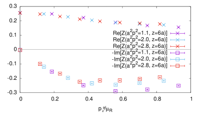
Figure 1: The NPR $Z=Z_{mp}$ (top) and $\delta Z=Z_{\not{p}}-Z_{mp}$ (bottom) at $z=6a$ ($\approx 0.5$ fm) as a function of $p_{z}^{R}/\mu_{R}=1/\sqrt{r}$, with various $\mu_{R}$. At $p_{z}^{R}=0$, $Z$ is real and $\delta Z/Z$ is less than 5%.

As shown in Eq. (II.2), the one-loop matching formula primarily depends on the combination $r=\mu^{2}_{R}/(p_{z}^{R})^{2}$ but is independent of $p^{R}_{t}$. In Fig. 1, the $Z_{mp}$ and $Z_{\not{p}}-Z_{mp}$ at fixed $z\sim 0.5$ fm are plotted as a function of $p^{R}_{z}/\mu_{R}=1/\sqrt{r}$. From this figure, one can see that the NPR factors, both real and imaginary parts, only show the dependence on $r$ regardless of the values of $p_{z}^{R}$ or $\mu_{R}$, with $p_{z}^{R}/\mu_{R}<0.4$.

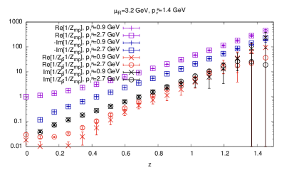
Figure 2: The inverse of the minimum projection renormalization factor $1/Z_{mp}$ and the difference $1/Z_{\not{p}}-1/Z_{mp}$, as a function of $z$ with the same $p^{R}_{z}$ and $\mu_{R}$, but different $p^{R}_{t}$. The crosses correspond to $p_{t}^{R}=0.9$ GeV and the open boxes (circles) are for $p_{t}^{R}=2.7$ GeV. Most results show mild dependence on $p^{R}_{t}$.

In Fig. 2, we show $1/Z_{mp}$ and $1/Z_{\not{p}}-1/Z_{mp}$ as functions of the Wilson link length $z$, with the same $\mu_{R}$=3.2 GeV and $p_{z}^{R}=1.4$ GeV and two different values of $p_{t}^{R}$=0.9 GeV and 2.7 GeV. As shown in this figure, the $1/Z_{mp}$ and $1/Z_{\not{p}}-1/Z_{mp}$ with the two different $p_{t}^{R}$’s are close to each other for all $z$ (the curves with the same color). This is consistent with the 1-loop matching formula. At $z<0.3$ fm, the real part of $1/Z_{\not{p}}-1/Z_{mp}$ with the two different $p_{t}^{R}$’s can be slightly nonzero, but it is still smaller than $1/Z_{\not{p}}$ by two orders of magnitude.

In the following we will take $p_{z}^{R}$ to be zero and estimate the systematic uncertainty from the $p_{z}^{R}$ dependence by varying the $p_{z}^{R}$.

In the calculation of nucleon matrix element, we use Gaussian momentum smearing Bali:2016lva for the quark field

$$\psi(x)\to S_{\text{mom}}\psi(x)=\frac{1}{1+6\alpha}$$

$$\left[\psi(x)+\alpha\sum_{j}U^{APE}_{j}(x)e^{ik\hat{e}_{j}}\psi(x+\hat{e}_{j})\right]\,,$$ (58)

where $k$ is the desired momentum, $U^{APE}_{j}(x)$ are the APE smeared gauge links in the $j$ direction, and $\alpha$ is a tunable parameter as in traditional Gaussian smearing.

Such a momentum source is designed to increase the overlap with nucleons of the desired boost momentum and we are able to reach higher-boosted momentum for the nucleon states than in the previous work Chen:2017mzz . Although in the exploratory study, we varied the Gaussian smearing radius to better overlap with the largest momentum used in the calculation, the field smearing is still centered around zero momentum in momentum space. When we switch to the momentum smearing, the smearing center will be shifted to momentum $O(k)$, which will immediately allow us to reach higher boost momenta with better signal-to-noise ratios in the matrix elements. In this work, we use two values of nucleon boost momenta, $P_{z}=n\frac{2\pi}{L}$, with $n\in\{4,5\}$, which corresponds to 1.8 and 2.3 GeV.

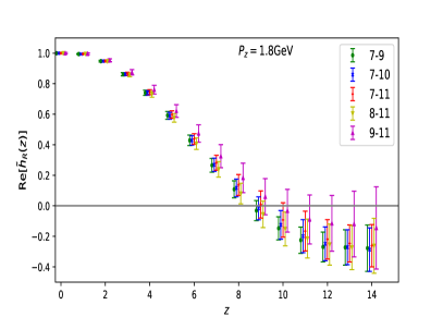
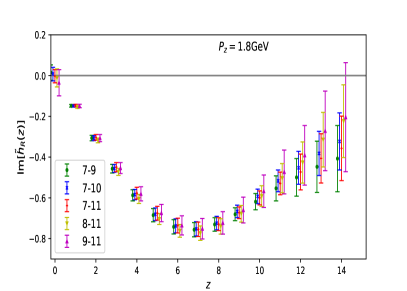
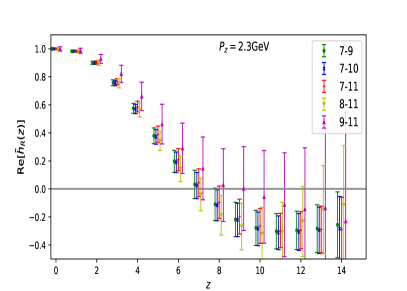
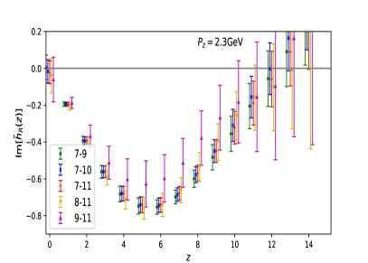
Figure 3: The real (left) and imaginary (right) parts of the isovector nucleon matrix elements for unpolarized PDFs as functions of $z$ at different momenta, with $P_{z}=\frac{8\pi}{L}$=1.8 GeV (top) and $\frac{10\pi}{L}=$2.3 GeV (bottom) respectively. The RI/MOM renormalization factors with $\{\mu,p_{z}^{R}\}=\{3.2,0\}$ GeV and the normalization at $z=0$ are applied on the bare matrix elements to improve the visibility at large $z$. At a given positive $z$ value, the data is slightly offset to show the ground-state matrix element from the fits using different ranges; from left to right they are: $t_{\text{seq}}\in$ [7,9], [7,10], [7,11], [8,11], and [9,11]. Different analyses are consistent within statistical errors while the fits with separation 7 and 8 have smaller uncertainties compared to other cases.

On the Lattice, we calculate the time-independent and nonlocal in $z$ direction correlators of a nucleon with finite-$P_{z}$ boost

$$\widetilde{h}_{\text{lat}}(z,P_{z},{\Gamma};a^{-1})=\left\langle 0;\vec{P}\right|O_{\Gamma}(z)\left|0;\vec{P}\right\rangle.$$ (59)

Here the state $|0;\vec{P}\rangle$ represents the ground (nucleon) state with momentum $\vec{P}=\{0,0,P_{z}\}$. $\Gamma=\gamma^{t}$ is used for the unpolarized parton distribution.

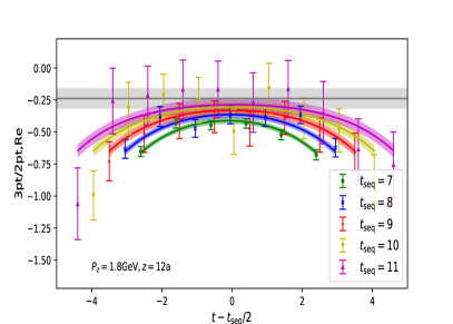
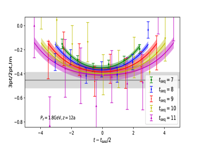
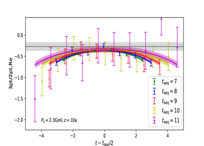
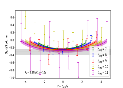
Figure 4: The real (left) and imaginary (right) parts of the renormalized isovector nucleon matrix elements for unpolarized PDFs with ${P_{z},z}={8\pi/L,12}$ (top) and ${10\pi/L,10}$ (bottom) which correspond to $zP_{z}\sim 9.5$. The data points and the band predicted by the fit using $t_{\text{seq}}\in$ [7, 11] agree with each other well.

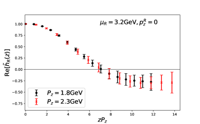
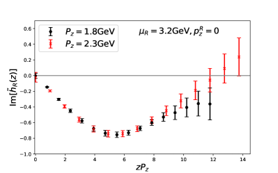
Figure 5: The renormalized quasi-PDF matrix elements with $P_{z}=$1.8 and 2.3 GeV, using the minimal projection with $p_{z}^{R}=0$ and $\mu_{R}=3.2$ GeV, as function of $zP_{z}$.

As the nucleon boost momentum increases, one anticipates that excited-state contributions are more severe; therefore, a careful study of the excited-state contamination is necessary. To do so, we calculate the nucleon matrix element $\widetilde{h}_{\rm lat}$ at five source-sink separations $t_{\text{seq}}\in\{7,8,9,10,11\}\times 0.086$ fm, with $\{4,4,8,8,16\}$ measurements on each of 2005 gauge configurations respectively in the $P_{z}=1.8$ GeV case, and of 2,000 configurations in the $P_{z}=2.3$ GeV case. We use a multigrid algorithm Babich:2010qb ; Osborn:2010mb with the Chroma software package Edwards:2004sx to speed up the inversion of the quark propagator. Following Ref. Bhattacharya:2013ehc , each three-point (3pt) correlator $C_{\Gamma}^{(3\text{pt})}(t,t_{\text{seq}})$ can be decomposed as (assuming the source is at $t=0$)

$$C^{\text{3pt}}(t,t_{\text{seq}};P_{z},{\Gamma}) ={\cal A}_{0}^{2}\langle 0|O_{\Gamma}|0\rangle e^{-E_{0}t_{\text{seq}}}$$ (60)

$$+{\cal A}_{1}^{2}\langle 1|O_{\Gamma}|1\rangle e^{-E_{1}t_{\text{seq}}}$$

$$+{\cal A}_{1}{\cal A}_{0}\langle 1|O_{\Gamma}|0\rangle e^{-E_{1}(t_{\text{seq}}-t)}e^{-E_{0}t}$$

$$+{\cal A}_{0}{\cal A}_{1}\langle 0|O_{\Gamma}|1\rangle e^{-E_{0}(t_{\text{seq}}-t)}e^{-E_{1}t}+\ldots\,,$$

where $|n\rangle$ with $n>0$ represents the excited states. The operator is inserted at time $t$, and the nucleon state is annihilated at the sink time $t_{\text{seq}}$( which is also the source-sink separation). The spectrum weights ${\cal A}_{0,1}$ and energies $E_{0,1}$ in Eq. (61) can be obtained from the two-point (2pt) correlator:

$$C^{\text{2pt}}(t_{\text{seq}};P_{z}) ={\cal A}_{0}^{2}e^{-E_{0}t_{\text{seq}}}+{\cal A}_{1}^{2}e^{-E_{1}t_{\text{seq}}}+\ldots\ .$$ (61)

Eventually we apply the joint fit with the 3pt functions at several $t_{\text{seq}}$ and 2pt function using the following form Bhattacharya:2013ehc :

$$\frac{C^{\text{3pt}}(t,t_{\text{seq}})}{C^{\text{2pt}}(t_{\text{seq}})}=$$

$$=\frac{\tilde{h}_{\text{lat}}+C_{2}(e^{-\Delta Et}+e^{-\Delta E(t_{\text{seq}}-t)})+C_{3}e^{-\Delta Et_{\text{seq}}}}{1+C_{1}e^{-\Delta Et_{\text{seq}}}},$$

$$C^{\text{2pt}}(t)=C_{0}e^{-E_{0}t}(1+C_{1}e^{-\Delta Et}),$$ (62)

with $\Delta E=E_{1}-E_{0}$. $C_{0,1,2,3}$ and $E_{0,1}$ are free parameters. We limit the range of $t$ as $t\in[1,t_{\text{seq}}-1]$ for 3pt/2pt ratio and $t\in[7,11]$ for the 2pt to make the $\chi^{2}/d.o.f.$ of the fit to be ${\cal O}(1)$. Using the ratio of 3pt/2pt instead of the 3pt function itself can improve the stability of the fit, especially when $C^{\text{2pt}}(t)$ with $t<7$ is included in the fit.

In Fig. 3, we show the ground-state nucleon matrix elements $\tilde{h}_{lat}(z,P_{z},\gamma_{t})$ obtained from five fits: using the separations $t_{\text{seq}}\in$ [7, 9], [7, 10], [7,11], [8,11], and [9,11] (The data points correspond to the same $z$ but are shifted horizontally to enhance the visibility). The data are further normalized by multiplying the renormalization factor with $\{\mu_{R},p_{z}^{R}\}=\{3.2,0\}$ GeV and the real part normalized to 1 at $z=0$. From this figure, one can see that there is no clear signal for excited-state contributions in any of these analyses. If the data with smallest two separations are dropped, uncertainties are getting much larger. In the fit, we keep the $C_{3}$ term to make a moderate estimate of the uncertainty even when this term is not statistically significant.

For a comparison between data and the fit, we show our results at large $z$ like $({P_{z},z})=({8\pi/L,12a})$ and $({10\pi/L,10a})$ with $t_{\text{seq}}\in$ [7,11] in Fig. 4. In these spatial separations, the real part of matrix element seems to be negative. The ground-state contribution obtained from the fit is shown as the black band. As one can see, most data can be well described in the fit and thereby we use the two-state fits and the interval $t_{\text{seq}}\in$ [7, 11] to obtain the results in the rest part of this paper.

The renormalized quasi-PDF matrix elements with two values of $P_{z}$ are plotted in Fig. 5, as function of $zP_{z}$ for $p^{R}_{z}=0$ and $\mu_{R}=3.2$ GeV. The results with different $P_{z}$ are consistent with each other within statistical uncertainties. This indicates that power corrections due to higher-twist effects might not be sizable.

III.2 Systematic Uncertainties

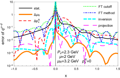
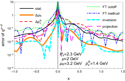
Figure 6: Different contributions to the systematic errors. See the text for detailed information.

In this subsection, we will consider four systematic uncertainties from: Fourier transformation (FT), unphysical scales $p_{z}^{R}$ and $\mu_{R}$, projection used in the RI/MOM scheme, and inversion of the matching coefficient.

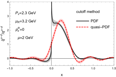
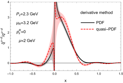
Figure 7: The quasi-PDF (dashed-red) with nucleon boost momentum 2.3 GeV and matched PDF (solid-black) at $\mu=2$ GeV using minimal projection, with the RI/MOM parameters $p_{z}^{R}=0$ and $\mu_{R}=3.2$ GeV. The upper and lower figures are obtained using the derivative and cutoff methods to perform Fourier transformation. The matching strategy has an important impact on the final results for PDFs.

In the following, we explain the details to include these systematic uncertainties.

1) Fourier transformation. As shown in Fig. 5, the $\widetilde{h}_{R}(z)$ with $P_{z}$=2.3 GeV is consistent with zero when $z>12a$. Thus in the standard matching from quasi-PDF to PDF, it is reasonable to truncate the results at $z=12a$. With this spirit, the quasi-PDF and matched PDF using the standard FT are shown in the upper panel of Fig. 7, from which one can see the matched PDF shows an oscillatory behavior. A “derivative” method was proposed in Ref.  Lin:2017ani to cure this oscillatory behavior. To be concrete, one takes the derivative of the renormalized nucleon matrix elements $\partial_{z}\widetilde{h}_{R}(z)$, whose Fourier transform differs from the original matrix element in a known way:

$$\widetilde{q}_{R}(x)=\int^{\infty}_{-\infty}\frac{dz}{2\pi}\frac{ie^{ixP_{z}z}}{x}\partial_{z}\widetilde{h}_{R}(z),$$ (63)

provided that $\widetilde{h}_{R}(z)$ goes to zero as $|z|\to\infty$. With the same truncation, the result is shown in the lower panel of Fig. 7 and apparently the oscillatory behavior is less severe. Besides, results obtained using the derivative method is consistent with the standard FT method in most kinematics region except at small $x$. This is anticipated as two methods only differ at the large $z$ region where we have made the truncation. We show the difference as the dot-dashed-blue line in Fig. 6, together with the error from varying the truncation from $z=10a$ to $14a$ (dotted-green line).

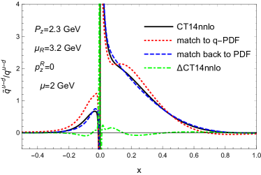
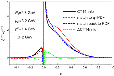
Figure 8: Effects of inversion matching formula using minimal projection: The solid-black, dotted-red, dotted-blue, and dot-dashed-green lines represent CT14nnlo PDF, applying inverse matching from CT14nnlo PDF Dulat:2015mca to quasi-PDF, applying matching again to get back to the PDF, the difference between PDF with iterative matching and the original CT14nnlo PDF. The upper (lower) figure corresponds to $p_{z}^{R}=0$ (1.4 GeV). These plots show that the method we used to invert the matching formula is less reliable for small $|x|$. The difference shown by the dot-dashed-green curve is taken into account into our systematic error.

2) Unphysical scales $p_{z}^{R}$ and $\mu_{R}$. There are two unphysical scales $p_{z}^{R}$ and $\mu_{R}$ introduced in RI/MOM. In principle, when matching the quasi-PDF matrix element onto lightcone PDF, the dependence on these two scales in the matrix element should exactly cancel with that in the matching kernel. However, since the quasi-PDF matrix element is non-perturbatively renormalized on the Lattice, while the matching coefficient is calculated at one-loop order in perturbation theory, there will be residual dependence on these two scales after the perturbative matching. To estimate the residual $p_{z}^{R}$ and $\mu_{R}$ dependence, we choose $p_{z}^{R}=0$ GeV and $\mu_{R}=3.2$ GeV as the central value, and vary $p_{z}^{R}$ from -1.4 to 1.4 GeV (dashed-red line) and $\mu_{R}$ from 2.4 to 3.9 GeV (thick-solid-orange line). The difference between these matched PDFs is treated as the systematics of the residual dependence on unphysical scales, in Fig. 6. As shown in the figure, the systematic uncertainty due to the $\mu_{R}$ dependence is small compared to the other sources, but the residual $p_{z}^{R}$ dependence could be sizable.

3) Dependencies on the projection. There are two projections discussed in this work: the minimum and “$\not{p}$” projections. With $p_{z}^{R}=0$, the projection dependence in both the NPR factor are less than 5% for all the $z$, and vanishes in the 1-loop perturbative matching. Thus one can expect that the difference due to the projections is also small, as depicted in the long-dashed-magenta lines in Fig. 6.

4) Inversion of matching. To extract the PDF from the quasi-PDF, one needs to invert the factorization formula Eq. (I). This could be done by changing the sign of $\alpha_{s}$ in $C$, and convoluting the new matching coefficient with $\widetilde{q}$. More explicitly, we have

$$q(x,\mu)= \int_{-\infty}^{\infty}{dy\over|y|}\>C^{\prime}\left({x\over y},r,\frac{yP_{z}}{\mu},\frac{yP_{z}}{p_{z}^{R}}\right)\widetilde{q}(y,P_{z},p^{R}_{z},\mu_{R})$$

$$+\mathcal{O}\left({M^{2}\over P_{z}^{2}},{\Lambda_{\text{QCD}}^{2}\over x^{2}P_{z}^{2}},\alpha_{s}^{2}\right)\,,$$ (64)

where $C^{\prime}=C(\alpha_{s}\to-\alpha_{s})$. We estimate the error due to inverting the factorization formula by starting from the PDF from a global analysis Dulat:2015mca , applying Eq.(I) and then Eq. (III.2) to return to the PDF. This manipulation should give the same lightcone PDF. However, since the matching is only accurate up to $O(\alpha_{s})$, the two results would differ, and the difference gives a good estimate of the systematic error coming from the inversion and higher order corrections. This is shown in Fig. 8, from which one can find that the error only becomes sizable when $|x|$ is small. This is expected because the relevant momentum scale is $xP^{z}$ such that higher order corrections become large at small $x$.

There are more sophisticated methods to invert the factorization, such as using a recursion procedure. However, as we can see in Fig. 6, the systematic error caused by the matching procedure (thick-dashed-cyan line) is also smaller than those from the first two sources in most regions.

As shown in Fig. 6, one can find that the dominant uncertainties arise from the $p_{z}^{R}$ dependence and from FT. With $p_{z}^{R}=0$, the uncertainties from different projections, and inversion and the matching are typically less than $10\%$ except in the region with very small $|x|$. The uncertainty from the $\mu_{R}$ dependence is even smaller. With $p_{z}^{R}=1.4$ GeV, uncertainties from these three sources are getting larger in magnitude, but still smaller than those from the two major sources.

IV Final Results for PDF

Figure 9: Nucleon boost momentum dependence of the matched unpolarized isovector PDFs: the dotted-green and solid-blue lines correspond to the nucleon momentum $P_{z}$ to be 1.8 and 2.3 GeV, respectively. The cutoff of Fourier transformation is chosen to be $zP^{z}\sim 12$ ($z=15a$ for $P_{z}=1.8$ GeV and $z=12a$ for $P_{z}=2.3$ GeV).

With the derivative method of FT and the matching using $p_{z}^{R}=0$ GeV and $\mu_{R}=3.2$ GeV, we show the dependence on the nucleon boosted momentum in Fig. 9 with the statistical uncertainties. They are consistent with each other as we can expect from the consistency of the quasi-PDF matrix element results in Fig. 5.

Finally, we show our results for PDF and a comparison with global-analysis Dulat:2015mca ; Ball:2017nwa ; Harland-Lang:2014zoa in Fig. 10. As can be seen from the plot, our results show a reasonable agreement in the large-$x$ region, but at small-$x$ region there exists notable difference majorly due to the systematic uncertainties from the FT truncation method and also the $p_{z}^{R}$ dependence.

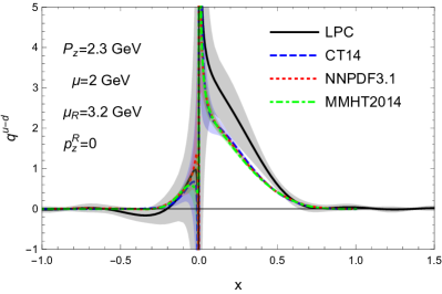
Figure 10: Results for PDF at $\mu=2$ GeV calculated from RI/MOM quasi-PDF at nucleon momentum $P_{z}=2.3$ GeV: Comparing with CT14nnlo (90CL) Dulat:2015mca , NNPDF3.1 (68CL) Ball:2017nwa , and MMHT2014 (68CL) Harland-Lang:2014zoa . Our results agree with the global-analysis within uncertainties.

V Summary

In this paper, we have studied the quasi-PDF defined with $\gamma^{t}$ which is free from mixing at $\mathcal{O}(a^{0})$. We have used $M_{\pi}=356$ MeV Lattice data to demonstrate the matching procedure and show that the excited state contamination is well under control. The one-loop matching coefficient is calculated and we have discussed the sources of systematic errors as well as the choice of the projection in detail.

We have found that the systematic uncertainties from the FT truncation method and also the $p_{z}^{R}$ dependence are sizable. But those uncertainties from $\mu_{R}$, inversion of matching and choice of projection are relatively minor with $p_{z}^{R}$=0. At the same time, the significant change from quasi-PDF to matched PDF suggests that higher-loop corrections are needed as exhibited in Fig. 7.

Controlling systematic uncertainty from the excited state is very challenging since the relative uncertainty grows very fast when either source-sink separation $t_{\text{seq}}$ or nucleon momentum $P_{z}$ become large. The two-state fit with smaller separation provides a possibility to obtain a precise result in small $t_{\text{seq}}<1$fm region, while for an accurate measurement at large separation using very high statistics, estimating the systematic uncertainty of such a fit is still needed.

Besides the uncertainties that we have studied, in the future we plan to investigate other systematics such as Lattice discretization and finite volume effects Lin:2019ocg as well as higher twist contributions that affect the small-$x$ result. The latter can be improved with larger nucleon momentum and estimated by extrapolating to infinite nucleon momentum.

Our final result for lightcone PDF agrees with the global analysis in the large-$x$ region, which gives an encouraging signal that LaMET may allow us to precisely access parton physics in the future.

Appendix

.1 One-loop quasi-PDF with $\gamma^{\alpha}$ in general covariant gauge

The gluon propagator in the general covariant gauge is

$$iD_{\tau}^{\mu\nu}(k)=-\frac{i}{k^{2}}\left[g^{\mu\nu}-(1-\tau)\frac{k^{\mu}k^{\nu}}{k^{2}}\right]\,.$$ (65)

For general $\Gamma=\gamma^{\alpha}$, the one-loop result can be expressed as

$$\widetilde{q}^{(1)}(x,p,\rho)=\mbox{Tr}\left[\left(\left[\widetilde{f}_{\alpha}(x,\rho)\right]_{+}\gamma^{\alpha}+\left[\widetilde{f}_{z}(x,\rho)\right]_{+}\frac{p_{\alpha}}{p_{z}}\gamma^{z}+\left[\widetilde{f}_{p}(x,\rho)\right]_{+}\frac{p_{\alpha}\not{p}}{p^{2}}\right){\cal P}\right]\,,$$ (66)

where

$$\widetilde{f}_{\alpha}(x,\rho) =\frac{\alpha_{s}C_{F}}{2\pi}\left\{\begin{array}[]{lc}\frac{x-\rho}{(1-x)(1-\rho)}+\frac{2x(2-x)-\rho(1+x)}{2(1-x)(1-\rho)^{3/2}}\ln\frac{2x-1+\sqrt{1-\rho}}{2x-1-\sqrt{1-\rho}}&x>1\\ \frac{-3x+2x^{2}+\rho}{(1-x)(1-\rho)}+\frac{2x(2-x)-\rho(1+x)}{2(1-x)(1-\rho)^{3/2}}\ln\frac{1+\sqrt{1-\rho}}{1-\sqrt{1-\rho}}&0<x<1\\ -\frac{x-\rho}{(1-x)(1-\rho)}-\frac{2x(2-x)-\rho(1+x)}{2(1-x)(1-\rho)^{3/2}}\ln\frac{2x-1+\sqrt{1-\rho}}{2x-1-\sqrt{1-\rho}}&x<0\end{array}\right.$$ (70)

$$+\frac{\alpha_{s}C_{F}}{2\pi}(1-\tau)\left\{\begin{array}[]{lc}\frac{\rho(-3x+2x^{2}+\rho)}{2(1-x)(1-\rho)(4x-4x^{2}-\rho)}+\frac{-\rho}{4(1-\rho)^{3/2}}\ln\frac{2x-1+\sqrt{1-\rho}}{2x-1-\sqrt{1-\rho}}&x>1\\ \frac{-x+\rho}{2(1-x)(1-\rho)}+\frac{-\rho}{4(1-\rho)^{3/2}}\ln\frac{1+\sqrt{1-\rho}}{1-\sqrt{1-\rho}}&0<x<1\\ -\frac{\rho(-3x+2x^{2}+\rho)}{2(1-x)(1-\rho)(4x-4x^{2}-\rho)}-\frac{-\rho}{4(1-\rho)^{3/2}}\ln\frac{2x-1+\sqrt{1-\rho}}{2x-1-\sqrt{1-\rho}}&x<0\end{array}\right.,$$ (74)

$$\widetilde{f}_{z}(x,\rho) =\frac{\alpha_{s}C_{F}}{2\pi}\left\{\begin{array}[]{lc}\begin{array}[]{l}\frac{-2\rho(1-7x+6x^{2})-\rho^{2}(1+2x)}{(1-\rho)^{2}(4x-4x^{2}-\rho)}g_{z\alpha}+\frac{4x(1-3x+2x^{2})-\rho(2-11x+12x^{2}-4x^{3})-\rho^{2}}{(1-x)(1-\rho)^{2}(4x-4x^{2}-\rho)}\\ \quad+\left[\frac{\rho(4-6x-\rho)}{2(1-\rho)^{5/2}}g_{z\alpha}+\frac{2-4x+4x^{2}-5x\rho+2x^{2}\rho+\rho^{2}}{2(1-x)(1-\rho)^{5/2}}\right]\ln\frac{2x-1+\sqrt{1-\rho}}{2x-1-\sqrt{1-\rho}}\end{array}&x>1\\ \begin{array}[]{l}\frac{-2+2x-\rho(1-4x)}{(1-\rho)^{2}}g_{z\alpha}+\frac{(-1+2x)(2-3x+\rho)}{(1-x)(1-\rho)^{2}}\\ \quad+\left[\frac{\rho(4-6x-\rho)}{2(1-\rho)^{5/2}}g_{z\alpha}+\frac{2-4x+4x^{2}-5x\rho+2x^{2}\rho+\rho^{2}}{2(1-x)(1-\rho)^{5/2}}\right]\ln\frac{1+\sqrt{1-\rho}}{1-\sqrt{1-\rho}}\end{array}&0<x<1\\ \begin{array}[]{l}-\frac{-2\rho(1-7x+6x^{2})-\rho^{2}(1+2x)}{(1-\rho)^{2}(4x-4x^{2}-\rho)}g_{z\alpha}-\frac{4x(1-3x+2x^{2})-\rho(2-11x+12x^{2}-4x^{3})-\rho^{2}}{(1-x)(1-\rho)^{2}(4x-4x^{2}-\rho)}\\ \quad-\left[\frac{\rho(4-6x-\rho)}{2(1-\rho)^{5/2}}g_{z\alpha}+\frac{2-4x+4x^{2}-5x\rho+2x^{2}\rho+\rho^{2}}{2(1-x)(1-\rho)^{5/2}}\right]\ln\frac{2x-1+\sqrt{1-\rho}}{2x-1-\sqrt{1-\rho}}\end{array}&x<0\end{array}\right.$$ (84)

$$+\frac{\alpha_{s}C_{F}}{2\pi}(1-\tau)\left\{\begin{array}[]{lc}\begin{array}[]{l}\frac{\rho(1-2x)[-4x(1-x)(2+\rho)+3\rho^{2}]}{2(1-\rho)^{2}(4x-4x^{2}-\rho)^{2}}g_{z\alpha}+\frac{\rho[-4x(2-9x+6x^{2})+\rho(1-10x+2\rho)]}{2(1-\rho)^{2}(4x-4x^{2}-\rho)^{2}}\\ \quad+\frac{\rho[(2+\rho)g_{z\alpha}+3)]}{4(1-\rho)^{5/2}}\ln\frac{2x-1+\sqrt{1-\rho}}{2x-1-\sqrt{1-\rho}}\end{array}&x>1\\ \frac{-3\rho g_{z\alpha}-1-2\rho}{2(1-\rho)^{2}}+\frac{\rho[(2+\rho)g_{z\alpha}+3)]}{4(1-\rho)^{5/2}}\ln\frac{1+\sqrt{1-\rho}}{1-\sqrt{1-\rho}}&0<x<1\\ \begin{array}[]{l}-\frac{\rho(1-2x)[-4x(1-x)(2+\rho)+3\rho^{2}]}{2(1-\rho)^{2}(4x-4x^{2}-\rho)^{2}}g_{z\alpha}-\frac{\rho[-4x(2-9x+6x^{2})+\rho(1-10x+2\rho)]}{2(1-\rho)^{2}(4x-4x^{2}-\rho)^{2}}\\ \quad-\frac{\rho[(2+\rho)g_{z\alpha}+3)]}{4(1-\rho)^{5/2}}\ln\frac{2x-1+\sqrt{1-\rho}}{2x-1-\sqrt{1-\rho}}\end{array}&x<0\end{array}\right.,$$ (92)

$$\widetilde{f}_{p}(x,\rho) =\frac{\alpha_{s}C_{F}}{2\pi}\left\{\begin{array}[]{lc}\begin{array}[]{l}\frac{-4x\rho(3-5x+2x^{2})+\rho^{2}(4-3x+4x^{2}-4x^{3})-\rho^{3}}{(1-x)(1-\rho)^{2}(4x-4x^{2}-\rho)}g_{z\alpha}+\frac{-2x\rho(5-6x)+\rho^{2}(3-2x)}{(1-\rho)^{2}(4x-4x^{2}-\rho)}\\ \quad+\left[\frac{-2\rho(1-4x+2x^{2})-\rho^{2}(2-x+2x^{2})+\rho^{3}}{2(1-x)(1-\rho)^{5/2}}g_{z\alpha}+\frac{-\rho(2-6x+\rho)}{2(1-\rho)^{5/2}}\right]\ln\frac{2x-1+\sqrt{1-\rho}}{2x-1-\sqrt{1-\rho}}\end{array}&x>1\\ \begin{array}[]{l}\frac{\rho(1-2x)(4-3x-\rho)}{(1-x)(1-\rho)^{2}}g_{z\alpha}+\frac{-2x+3\rho-4x\rho}{(1-\rho)^{2}}\\ \quad+\left[\frac{-\rho(2-8x+4x^{2})-\rho^{2}(2-x+2x^{2})+\rho^{3}}{2(1-x)(1-\rho)^{5/2}}g_{z\alpha}+\frac{-\rho(2-6x+\rho)}{2(1-\rho)^{5/2}}\right]\ln\frac{1+\sqrt{1-\rho}}{1-\sqrt{1-\rho}}\end{array}&0<x<1\\ \begin{array}[]{l}-\frac{-4x\rho(3-5x+2x^{2})+\rho^{2}(4-3x+4x^{2}-4x^{3})-\rho^{3}}{(1-x)(1-\rho)^{2}(4x-4x^{2}-\rho)}g_{z\alpha}-\frac{-2x\rho(5-6x)+\rho^{2}(3-2x)}{(1-\rho)^{2}(4x-4x^{2}-\rho)}\\ \quad-\left[\frac{-2\rho(1-4x+2x^{2})-\rho^{2}(2-x+2x^{2})+\rho^{3}}{2(1-x)(1-\rho)^{5/2}}g_{z\alpha}+\frac{-\rho(2-6x+\rho)}{2(1-\rho)^{5/2}}\right]\ln\frac{2x-1+\sqrt{1-\rho}}{2x-1-\sqrt{1-\rho}}\end{array}&x<0\end{array}\right.$$ (102)

$$+\frac{\alpha_{s}C_{F}}{2\pi}(1-\tau)\left\{\begin{array}[]{lc}\begin{array}[]{l}\frac{16x\rho(1-3x+2x^{2})+4x^{2}\rho^{2}(3-2x)-\rho^{3}(5-2x)+2\rho^{4}}{2(1-\rho)^{2}(4x-4x^{2}-\rho)^{2}}g_{z\alpha}\\ \quad+\frac{\rho(1-2x)[16x(1-x)-2\rho(1+2x-2x^{2})-\rho^{2}]}{2(1-\rho)^{2}(4x-4x^{2}-\rho)^{2}}+\frac{-\rho(4-\rho)(g_{z\alpha}+1)}{4(1-\rho)^{5/2}}\ln\frac{2x-1+\sqrt{1-\rho}}{2x-1-\sqrt{1-\rho}}\end{array}&x>1\\ \frac{\rho(5-2\rho)g_{z\alpha}+2+\rho}{2(1-\rho)^{2}}+\frac{-\rho(4-\rho)(g_{z\alpha}+1)}{4(1-\rho)^{5/2}}\ln\frac{1+\sqrt{1-\rho}}{1-\sqrt{1-\rho}}&0<x<1\\ \begin{array}[]{l}-\frac{16x\rho(1-3x+2x^{2})+4x^{2}\rho^{2}(3-2x)-\rho^{3}(5-2x)+2\rho^{4}}{2(1-\rho)^{2}(4x-4x^{2}-\rho)^{2}}g_{z\alpha}\\ \quad-\frac{\rho(1-2x)[16x(1-x)-2\rho(1+2x-2x^{2})-\rho^{2}]}{2(1-\rho)^{2}(4x-4x^{2}-\rho)^{2}}-\frac{-\rho(4-\rho)(g_{z\alpha}+1)}{4(1-\rho)^{5/2}}\ln\frac{2x-1+\sqrt{1-\rho}}{2x-1-\sqrt{1-\rho}}\end{array}&x<0\end{array}\right..$$ (110)

.2 One-loop quasi-PDF with $\Gamma=\gamma^{z}$ in Landau gauge

For $\Gamma=\gamma^{z}$, we can obtain the matching coefficient Eq. (II.2) using the general formula with similar definition of the minimal and $\not{p}$ projections in Sec. II.2. The bare matching coefficients are

$$f_{1,mp}\left(x,\frac{p_{z}}{\mu}\right)=f_{1,\not{p}}\left(x,\frac{p_{z}}{\mu}\right)=\frac{\alpha_{s}C_{F}}{2\pi}\left\{\begin{array}[]{lc}\displaystyle\frac{1+x^{2}}{1-x}\ln\frac{x}{x-1}+1&x>1\\ \displaystyle\frac{1+x^{2}}{1-x}\ln\frac{4x(1-x)p_{z}^{2}}{\mu^{2}}+\frac{2-5x+x^{2}}{1-x}&0<x<1\\ \displaystyle-\frac{1+x^{2}}{1-x}\ln\frac{x}{x-1}-1&x<0\end{array}\right.,$$ (114)

and the corresponding counterterms are

$$f_{2,mp}(x,r)=\frac{\alpha_{s}C_{F}}{2\pi}\left\{\begin{array}[]{lc}\frac{3r-(1-2x)^{2}}{2(r-1)(1-x)}-\frac{4x^{2}(2-3r+2x+4rx-12x^{2}+8x^{3})}{(r-1)(r-4x+4x^{2})^{2}}+\frac{2-3r+2x^{2}}{(r-1)^{3/2}(x-1)}\tan^{-1}\frac{\sqrt{r-1}}{2x-1}&x>1\\ \frac{1-3r+4x^{2}}{2(r-1)(1-x)}+\frac{-2+3r-2x^{2}}{(r-1)^{3/2}(1-x)}\tan^{-1}\sqrt{r-1}&0<x<1\\ -\frac{3r-(1-2x)^{2}}{2(r-1)(1-x)}+\frac{4x^{2}(2-3r+2x+4rx-12x^{2}+8x^{3})}{(r-1)(r-4x+4x^{2})^{2}}-\frac{2-3r+2x^{2}}{(r-1)^{3/2}(x-1)}\tan^{-1}\frac{\sqrt{r-1}}{2x-1}&x<0\end{array}\right.$$ (118)

$$f_{2,\not{p}}(x,r)=\frac{\alpha_{s}C_{F}}{2\pi}\left\{\begin{array}[]{lc}1+\frac{r}{2}\frac{r(3-4x)-8x(x-1)^{2}}{(x-1)(r-4x+4x^{2})^{2}}+\frac{-2+r-2x^{2}}{\sqrt{r-1}(x-1)}\tan^{-1}\frac{\sqrt{r-1}}{2x-1}&x>1\\ \frac{1-6x}{2(1-x)}+\frac{2-r+2x^{2}}{\sqrt{r-1}(1-x)}\tan^{-1}\sqrt{r-1}&0<x<1\\ -1-\frac{r}{2}\frac{r(3-4x)-8x(x-1)^{2}}{(x-1)(r-4x+4x^{2})^{2}}-\frac{-2+r-2x^{2}}{\sqrt{r-1}(x-1)}\tan^{-1}\frac{\sqrt{r-1}}{2x-1}&x<0\end{array}\right.\,.$$ (122)

The result was also calculated in Ref. Stewart:2017tvs . Although the matching coefficient with $\Gamma=\gamma^{z}$ is not useful for isovector unpolarized PDF because it suffers from operator mixing in renormalization procedure, it can be used for isovector helicity PDF due to different symmetry properties.

References

- (1) J. Butterworth et al., J. Phys. G 43, 023001 (2016) doi:10.1088/0954-3899/43/2/023001 [arXiv:1510.03865 [hep-ph]].
- (2) S. Alekhin, J. Blümlein, S. Moch and R. Placakyte, Phys. Rev. D 96, no. 1, 014011 (2017) doi:10.1103/PhysRevD.96.014011 [arXiv:1701.05838 [hep-ph]].
- (3) J. Gao, L. Harland-Lang and J. Rojo, Phys. Rept. 742, 1 (2018) doi:10.1016/j.physrep.2018.03.002 [arXiv:1709.04922 [hep-ph]].
- (4) J. Collins, Camb. Monogr. Part. Phys. Nucl. Phys. Cosmol. 32, 1 (2011).
- (5) G. Martinelli and C. T. Sachrajda, Phys. Lett. B 196, 184 (1987). doi:10.1016/0370-2693(87)90601-0
- (6) G. Martinelli and C. T. Sachrajda, Phys. Lett. B 217, 319 (1989). doi:10.1016/0370-2693(89)90874-5
- (7) W. Detmold, W. Melnitchouk and A. W. Thomas, Eur. Phys. J. direct 3, no. 1, 13 (2001) doi:10.1007/s1010501c0013 [hep-lat/0108002].
- (8) D. Dolgov et al. [LHPC and TXL Collaborations], Phys. Rev. D 66, 034506 (2002) doi:10.1103/PhysRevD.66.034506 [hep-lat/0201021].
- (9) X. Ji, Phys. Rev. Lett. 110, 262002 (2013) doi:10.1103/PhysRevLett.110.262002 [arXiv:1305.1539 [hep-ph]].
- (10) X. Ji, Sci. China Phys. Mech. Astron. 57, 1407 (2014) doi:10.1007/s11433-014-5492-3 [arXiv:1404.6680 [hep-ph]].
- (11) I. W. Stewart and Y. Zhao, Phys. Rev. D 97, no. 5, 054512 (2018) doi:10.1103/PhysRevD.97.054512 [arXiv:1709.04933 [hep-ph]].
- (12) T. Izubuchi, X. Ji, L. Jin, I. W. Stewart and Y. Zhao, Phys. Rev. D 98, no. 5, 056004 (2018) doi:10.1103/PhysRevD.98.056004 [arXiv:1801.03917 [hep-ph]].
- (13) Y. Q. Ma and J. W. Qiu, Phys. Rev. D 98, no. 7, 074021 (2018) doi:10.1103/PhysRevD.98.074021 [arXiv:1404.6860 [hep-ph]].
- (14) Y. Q. Ma and J. W. Qiu, Phys. Rev. Lett. 120, no. 2, 022003 (2018) doi:10.1103/PhysRevLett.120.022003 [arXiv:1709.03018 [hep-ph]].
- (15) H. W. Lin, J. W. Chen, S. D. Cohen and X. Ji, Phys. Rev. D 91, 054510 (2015) doi:10.1103/PhysRevD.91.054510 [arXiv:1402.1462 [hep-ph]].
- (16) C. Alexandrou, K. Cichy, V. Drach, E. Garcia-Ramos, K. Hadjiyiannakou, K. Jansen, F. Steffens and C. Wiese, Phys. Rev. D 92, 014502 (2015) doi:10.1103/PhysRevD.92.014502 [arXiv:1504.07455 [hep-lat]].
- (17) J. W. Chen, S. D. Cohen, X. Ji, H. W. Lin and J. H. Zhang, Nucl. Phys. B 911, 246 (2016) doi:10.1016/j.nuclphysb.2016.07.033 [arXiv:1603.06664 [hep-ph]].
- (18) C. Alexandrou, K. Cichy, M. Constantinou, K. Hadjiyiannakou, K. Jansen, F. Steffens and C. Wiese, Phys. Rev. D 96, no. 1, 014513 (2017) doi:10.1103/PhysRevD.96.014513 [arXiv:1610.03689 [hep-lat]].
- (19) J. H. Zhang, J. W. Chen, L. Jin, H. W. Lin, A. Schäfer and Y. Zhao, Phys. Rev. D 100, no. 3, 034505 (2019) doi:10.1103/PhysRevD.100.034505 [arXiv:1804.01483 [hep-lat]].
- (20) C. Alexandrou, K. Cichy, M. Constantinou, K. Jansen, A. Scapellato and F. Steffens, Phys. Rev. D 98, no. 9, 091503 (2018) doi:10.1103/PhysRevD.98.091503 [arXiv:1807.00232 [hep-lat]].
- (21) J. H. Zhang, J. W. Chen, X. Ji, L. Jin and H. W. Lin, Phys. Rev. D 95, no. 9, 094514 (2017) doi:10.1103/PhysRevD.95.094514 [arXiv:1702.00008 [hep-lat]].
- (22) J. H. Zhang et al. [LP3 Collaboration], Nucl. Phys. B 939, 429 (2019) doi:10.1016/j.nuclphysb.2018.12.020 [arXiv:1712.10025 [hep-ph]].
- (23) X. Xiong, X. Ji, J. H. Zhang and Y. Zhao, Phys. Rev. D 90, no. 1, 014051 (2014) doi:10.1103/PhysRevD.90.014051 [arXiv:1310.7471 [hep-ph]].
- (24) X. Ji, A. Schäfer, X. Xiong and J. H. Zhang, Phys. Rev. D 92, 014039 (2015) doi:10.1103/PhysRevD.92.014039 [arXiv:1506.00248 [hep-ph]].
- (25) X. Xiong and J. H. Zhang, Phys. Rev. D 92, no. 5, 054037 (2015) doi:10.1103/PhysRevD.92.054037 [arXiv:1509.08016 [hep-ph]].
- (26) H. N. Li, Phys. Rev. D 94, no. 7, 074036 (2016) doi:10.1103/PhysRevD.94.074036 [arXiv:1602.07575 [hep-ph]].
- (27) G. C. Rossi and M. Testa, Phys. Rev. D 96, no. 1, 014507 (2017) doi:10.1103/PhysRevD.96.014507 [arXiv:1706.04428 [hep-lat]].
- (28) G. Rossi and M. Testa, Phys. Rev. D 98, no. 5, 054028 (2018) doi:10.1103/PhysRevD.98.054028 [arXiv:1806.00808 [hep-lat]].
- (29) X. Ji and J. H. Zhang, Phys. Rev. D 92, 034006 (2015) doi:10.1103/PhysRevD.92.034006 [arXiv:1505.07699 [hep-ph]].
- (30) T. Ishikawa, Y. Q. Ma, J. W. Qiu and S. Yoshida, arXiv:1609.02018 [hep-lat].
- (31) J. W. Chen, X. Ji and J. H. Zhang, Nucl. Phys. B 915, 1 (2017) doi:10.1016/j.nuclphysb.2016.12.004 [arXiv:1609.08102 [hep-ph]].
- (32) X. Xiong, T. Luu and U. G. Meißner, arXiv:1705.00246 [hep-ph].
- (33) M. Constantinou and H. Panagopoulos, Phys. Rev. D 96, no. 5, 054506 (2017) doi:10.1103/PhysRevD.96.054506 [arXiv:1705.11193 [hep-lat]].
- (34) X. Ji, J. H. Zhang and Y. Zhao, Phys. Rev. Lett. 120, no. 11, 112001 (2018) doi:10.1103/PhysRevLett.120.112001 [arXiv:1706.08962 [hep-ph]].
- (35) T. Ishikawa, Y. Q. Ma, J. W. Qiu and S. Yoshida, Phys. Rev. D 96, no. 9, 094019 (2017) doi:10.1103/PhysRevD.96.094019 [arXiv:1707.03107 [hep-ph]].
- (36) J. Green, K. Jansen and F. Steffens, Phys. Rev. Lett. 121, no. 2, 022004 (2018) doi:10.1103/PhysRevLett.121.022004 [arXiv:1707.07152 [hep-lat]].
- (37) G. Spanoudes and H. Panagopoulos, Phys. Rev. D 98, no. 1, 014509 (2018) doi:10.1103/PhysRevD.98.014509 [arXiv:1805.01164 [hep-lat]].
- (38) C. Alexandrou, K. Cichy, M. Constantinou, K. Hadjiyiannakou, K. Jansen, H. Panagopoulos and F. Steffens, Nucl. Phys. B 923, 394 (2017) doi:10.1016/j.nuclphysb.2017.08.012 [arXiv:1706.00265 [hep-lat]].
- (39) J. W. Chen, T. Ishikawa, L. Jin, H. W. Lin, Y. B. Yang, J. H. Zhang and Y. Zhao, Phys. Rev. D 97, no. 1, 014505 (2018) doi:10.1103/PhysRevD.97.014505 [arXiv:1706.01295 [hep-lat]].
- (40) G. Martinelli, C. Pittori, C. T. Sachrajda, M. Testa and A. Vladikas, Nucl. Phys. B 445, 81 (1995) doi:10.1016/0550-3213(95)00126-D [hep-lat/9411010].
- (41) H. W. Lin et al. [LP3 Collaboration], Phys. Rev. D 98, no. 5, 054504 (2018) doi:10.1103/PhysRevD.98.054504 [arXiv:1708.05301 [hep-lat]].
- (42) C. Alexandrou, K. Cichy, M. Constantinou, K. Jansen, A. Scapellato and F. Steffens, Phys. Rev. Lett. 121, no. 11, 112001 (2018) doi:10.1103/PhysRevLett.121.112001 [arXiv:1803.02685 [hep-lat]].
- (43) J. W. Chen, L. Jin, H. W. Lin, Y. S. Liu, Y. B. Yang, J. H. Zhang and Y. Zhao, arXiv:1803.04393 [hep-lat].
- (44) J. W. Chen et al. [LP3 Collaboration], Chin. Phys. C 43, no. 10, 103101 (2019) doi:10.1088/1674-1137/43/10/103101 [arXiv:1710.01089 [hep-lat]].
- (45) T. Ishikawa, L. Jin, H. W. Lin, A. Schäfer, Y. B. Yang, J. H. Zhang and Y. Zhao, Sci. China Phys. Mech. Astron. 62, no. 9, 991021 (2019) doi:10.1007/s11433-018-9375-1 [arXiv:1711.07858 [hep-ph]].
- (46) X. Ji, P. Sun, X. Xiong and F. Yuan, Phys. Rev. D 91, 074009 (2015) doi:10.1103/PhysRevD.91.074009 [arXiv:1405.7640 [hep-ph]].
- (47) X. Ji, L. C. Jin, F. Yuan, J. H. Zhang and Y. Zhao, Phys. Rev. D 99, no. 11, 114006 (2019) doi:10.1103/PhysRevD.99.114006 [arXiv:1801.05930 [hep-ph]].
- (48) M. A. Ebert, I. W. Stewart and Y. Zhao, Phys. Rev. D 99, no. 3, 034505 (2019) doi:10.1103/PhysRevD.99.034505 [arXiv:1811.00026 [hep-ph]].
- (49) M. A. Ebert, I. W. Stewart and Y. Zhao, JHEP 1909, 037 (2019) doi:10.1007/JHEP09(2019)037 [arXiv:1901.03685 [hep-ph]].
- (50) M. A. Ebert, I. W. Stewart and Y. Zhao, arXiv:1910.08569 [hep-ph].
- (51) X. Ji, Y. Liu and Y. S. Liu, arXiv:1910.11415 [hep-ph].
- (52) P. Shanahan, M. Wagman and Y. Zhao, arXiv:1911.00800 [hep-lat].
- (53) X. Ji, Y. Liu and Y. S. Liu, arXiv:1911.03840 [hep-ph].
- (54) W. Wang, S. Zhao and R. Zhu, Eur. Phys. J. C 78, no. 2, 147 (2018) doi:10.1140/epjc/s10052-018-5617-3 [arXiv:1708.02458 [hep-ph]].
- (55) W. Wang and S. Zhao, JHEP 1805, 142 (2018) doi:10.1007/JHEP05(2018)142 [arXiv:1712.09247 [hep-ph]].
- (56) Z. Y. Fan, Y. B. Yang, A. Anthony, H. W. Lin and K. F. Liu, Phys. Rev. Lett. 121, no. 24, 242001 (2018) doi:10.1103/PhysRevLett.121.242001 [arXiv:1808.02077 [hep-lat]].
- (57) J. H. Zhang, X. Ji, A. Schäfer, W. Wang and S. Zhao, Phys. Rev. Lett. 122, no. 14, 142001 (2019) doi:10.1103/PhysRevLett.122.142001 [arXiv:1808.10824 [hep-ph]].
- (58) Z. Y. Li, Y. Q. Ma and J. W. Qiu, Phys. Rev. Lett. 122, no. 6, 062002 (2019) doi:10.1103/PhysRevLett.122.062002 [arXiv:1809.01836 [hep-ph]].
- (59) W. Wang, J. H. Zhang, S. Zhao and R. Zhu, Phys. Rev. D 100, no. 7, 074509 (2019) doi:10.1103/PhysRevD.100.074509 [arXiv:1904.00978 [hep-ph]].
- (60) C. Monahan and K. Orginos, JHEP 1703, 116 (2017) doi:10.1007/JHEP03(2017)116 [arXiv:1612.01584 [hep-lat]].
- (61) C. Monahan, Phys. Rev. D 97, no. 5, 054507 (2018) doi:10.1103/PhysRevD.97.054507 [arXiv:1710.04607 [hep-lat]].
- (62) A. V. Radyushkin, Phys. Rev. D 96, no. 3, 034025 (2017) doi:10.1103/PhysRevD.96.034025 [arXiv:1705.01488 [hep-ph]].
- (63) K. Orginos, A. Radyushkin, J. Karpie and S. Zafeiropoulos, Phys. Rev. D 96, no. 9, 094503 (2017) doi:10.1103/PhysRevD.96.094503 [arXiv:1706.05373 [hep-ph]].
- (64) J. Karpie, K. Orginos, A. Radyushkin and S. Zafeiropoulos, EPJ Web Conf. 175, 06032 (2018) doi:10.1051/epjconf/201817506032 [arXiv:1710.08288 [hep-lat]].
- (65) X. Ji, J. H. Zhang and Y. Zhao, Nucl. Phys. B 924, 366 (2017) doi:10.1016/j.nuclphysb.2017.09.001 [arXiv:1706.07416 [hep-ph]].
- (66) J. H. Zhang, J. W. Chen and C. Monahan, Phys. Rev. D 97, no. 7, 074508 (2018) doi:10.1103/PhysRevD.97.074508 [arXiv:1801.03023 [hep-ph]].
- (67) K. F. Liu and S. J. Dong, Phys. Rev. Lett. 72, 1790 (1994) doi:10.1103/PhysRevLett.72.1790 [hep-ph/9306299].
- (68) J. Liang, K. F. Liu and Y. B. Yang, EPJ Web Conf. 175, 14014 (2018) doi:10.1051/epjconf/201817514014 [arXiv:1710.11145 [hep-lat]].
- (69) W. Detmold and C. J. D. Lin, Phys. Rev. D 73, 014501 (2006) doi:10.1103/PhysRevD.73.014501 [hep-lat/0507007].
- (70) V. Braun and D. Müller, Eur. Phys. J. C 55, 349 (2008) doi:10.1140/epjc/s10052-008-0608-4 [arXiv:0709.1348 [hep-ph]].
- (71) A. J. Chambers et al., Phys. Rev. Lett. 118, no. 24, 242001 (2017) doi:10.1103/PhysRevLett.118.242001 [arXiv:1703.01153 [hep-lat]].
- (72) G. S. Bali et al., Phys. Rev. D 98, no. 9, 094507 (2018) doi:10.1103/PhysRevD.98.094507 [arXiv:1807.06671 [hep-lat]].
- (73) G. S. Bali et al. [RQCD Collaboration], Eur. Phys. J. A 55, no. 7, 116 (2019) doi:10.1140/epja/i2019-12803-6 [arXiv:1903.12590 [hep-lat]].
- (74) C. E. Carlson and M. Freid, Phys. Rev. D 95, no. 9, 094504 (2017) doi:10.1103/PhysRevD.95.094504 [arXiv:1702.05775 [hep-ph]].
- (75) R. A. Briceño, M. T. Hansen and C. J. Monahan, Phys. Rev. D 96, no. 1, 014502 (2017) doi:10.1103/PhysRevD.96.014502 [arXiv:1703.06072 [hep-lat]].
- (76) M. Lüscher and S. Schäfer, JHEP 1107, 036 (2011) doi:10.1007/JHEP07(2011)036 [arXiv:1105.4749 [hep-lat]].
- (77) M. Bruno et al., JHEP 1502, 043 (2015) doi:10.1007/JHEP02(2015)043 [arXiv:1411.3982 [hep-lat]].
- (78) A. Hasenfratz and F. Knechtli, Phys. Rev. D 64, 034504 (2001) doi:10.1103/PhysRevD.64.034504 [hep-lat/0103029].
- (79) G. S. Bali, B. Lang, B. U. Musch and A. Schäfer, Phys. Rev. D 93, no. 9, 094515 (2016) doi:10.1103/PhysRevD.93.094515 [arXiv:1602.05525 [hep-lat]].
- (80) R. Babich, J. Brannick, R. C. Brower, M. A. Clark, T. A. Manteuffel, S. F. McCormick, J. C. Osborn and C. Rebbi, Phys. Rev. Lett. 105, 201602 (2010) doi:10.1103/PhysRevLett.105.201602 [arXiv:1005.3043 [hep-lat]].
- (81) J. C. Osborn, R. Babich, J. Brannick, R. C. Brower, M. A. Clark, S. D. Cohen and C. Rebbi, PoS Lattice 2010, 037 (2010) doi:10.22323/1.105.0037 [arXiv:1011.2775 [hep-lat]].
- (82) R. G. Edwards et al. [SciDAC and LHPC and UKQCD Collaborations], Nucl. Phys. Proc. Suppl. 140, 832 (2005) doi:10.1016/j.nuclphysbps.2004.11.254 [hep-lat/0409003].
- (83) T. Bhattacharya, S. D. Cohen, R. Gupta, A. Joseph, H. W. Lin and B. Yoon, Phys. Rev. D 89, no. 9, 094502 (2014) doi:10.1103/PhysRevD.89.094502 [arXiv:1306.5435 [hep-lat]].
- (84) S. Dulat et al., Phys. Rev. D 93, no. 3, 033006 (2016) doi:10.1103/PhysRevD.93.033006 [arXiv:1506.07443 [hep-ph]].
- (85) R. D. Ball et al. [NNPDF Collaboration], Eur. Phys. J. C 77, no. 10, 663 (2017) doi:10.1140/epjc/s10052-017-5199-5 [arXiv:1706.00428 [hep-ph]].
- (86) L. A. Harland-Lang, A. D. Martin, P. Motylinski and R. S. Thorne, Eur. Phys. J. C 75, no. 5, 204 (2015) doi:10.1140/epjc/s10052-015-3397-6 [arXiv:1412.3989 [hep-ph]].
- (87) H. W. Lin and R. Zhang, Phys. Rev. D 100, no. 7, 074502 (2019). doi:10.1103/PhysRevD.100.074502