Uniform estimate of an iterative method for elliptic problems with rapidly oscillating coefficients

Abstract

We study the iterative algorithm proposed by S. Armstrong, A. Hannukainen, T. Kuusi, J.-C. Mourrat in [3] to solve elliptic equations in divergence form with stochastic stationary coefficients. Such equations display rapidly oscillating coefficients and thus usually require very expensive numerical calculations, while this iterative method is comparatively easy to compute. In this article, we strengthen the estimate for the contraction factor achieved by one iteration of the algorithm. We obtain an estimate that holds uniformly over the initial function in the iteration, and which grows only logarithmically with the size of the domain.

1 Introduction

1.1 Main theorem

The problem of homogenization is a subject widely studied in mathematics and other disciplines for its applications and interesting properties. Let $(\mathbf{a}(x),x\in\mathbb{R}^{d})$ be a random coefficient field, which takes values in the set of $\mathbb{R}^{d\times d}$ symmetric matrices, and which we assume to be $\mathbb{Z}^{d}$-stationary, with a unit range of dependence and uniformly elliptic that $\Lambda^{-1}|\xi|^{2}\leqslant\xi\cdot\mathbf{a}(x)\xi\leqslant\Lambda|\xi|^{2}$ for any $x,\xi\in\mathbb{R}^{d}$. We give ourselves a bounded domain $U\subset\mathbb{R}^{d}$ with boundary $C^{1,1}$, a scale parameter $0<\varepsilon<1$, and for given $f\in H^{-1}(U)$ and $g\in H^{1}(U)$, we consider the elliptic Dirichlet problem

$$\left\{\begin{array}[]{ll}-\nabla\cdot\left(\mathbf{a}\left(\frac{\cdot}{\varepsilon}\right)\nabla u_{\varepsilon}\right)=f&\text{ in }U,\\ u_{\varepsilon}=g&\text{ on }\partial U.\end{array}\right.$$ (1.1)

For the scale $0<\varepsilon\ll 1$, a naive numerical algorithm for this problem is generally very expensive, due to the rapid oscillations of the coefficients (comparatively to the size of the domain) and we have to refine the mesh of the numerical schema. Thus, different methods have been proposed to approximate the solution and one of them is to replace the conductance matrix $\mathbf{a}$ by a constant effective conductance matrix $\bar{\mathbf{a}}$ in eq. 1.1 and use its solution $\bar{u}$ as an approximation, which can be solved quickly thanks to the multi-grid algorithm. However, $\bar{u}$ is close to $u_{\varepsilon}$ in the sense $L^{2}(U)$ or $H^{-1}(U)$, but not in some stronger topology, for example $H^{1}(U)$. Furthermore, the approximation only becomes accurate in the limit $\varepsilon\rightarrow 0$, but for a small finite scale $\varepsilon$, one can not expect a precision much smaller than $\varepsilon$ with $\bar{u}$.

Recently, [3] proposed an iterative algorithm to solve the problem eq. 1.2 efficiently for a given $\varepsilon$-scale and with a better precision. We recap at first their algorithm here with the same formulation in large scale: Instead of considering eq. 1.1 with a small scale $\varepsilon$, we treat the Dirichlet problem with a dilation parameter $r\geqslant 1$, and set $U_{r}:=rU$. Then given $f\in H^{-1}(U_{r})$ and $g\in H^{1}(U_{r})$, we consider the elliptic equation given by

$$\left\{\begin{array}[]{ll}-\nabla\cdot\mathbf{a}\nabla u=f&\text{ in }U_{r},\\ u=g&\text{ on }\partial U_{r},\end{array}\right.$$ (1.2)

and [3] proposes to start by an initial guess of solution $v\in g+H_{0}^{1}(U_{r})$, and solve $u_{0},\bar{u},\widetilde{u}\in H^{1}_{0}(U)$ satisfying (with null Dirichlet boundary condition)

$$\left\{\begin{array}[]{lll}(\lambda^{2}-\nabla\cdot\mathbf{a}\nabla)u_{0}&=f+\nabla\cdot\mathbf{a}\nabla v&\text{ in }U_{r},\\ -\nabla\cdot\bar{\mathbf{a}}\nabla\bar{u}&=\lambda^{2}u_{0}&\text{ in }U_{r},\\ (\lambda^{2}-\nabla\cdot\mathbf{a}\nabla)\widetilde{u}&=(\lambda^{2}-\nabla\cdot\bar{\mathbf{a}}\nabla)\bar{u}&\text{ in }U_{r}.\\ \end{array}\right.$$ (1.3)

Then, the iteration $\hat{v}:=v+u_{0}+\tilde{u}$ is a contraction. Since this rate of contraction is random, to estimate its size, [3] introduces the notation $\mathcal{O}_{s}$ for random variable $X$ that for any $s,\theta>0$,

$$X\leqslant\mathcal{O}_{s}(\theta)\Longleftrightarrow\operatorname{\mathbb{E}}\left[\exp(\max(\theta^{-1}X,0)^{s})\right]\leqslant 2.$$ (1.4)

Informally speaking, the statement $X\leqslant\mathcal{O}_{s}(1)$ tells us that $X$ has a tail lighter than $\exp(-x^{s})$. We also introduce the shorthand notation for every $\lambda\in(0,1]$,

$$\ell(\lambda):=\left\{\begin{array}[]{ll}(\log(1+\lambda^{-1}))^{\frac{1}{2}}&d=2,\\ 1&d>2.\end{array}\right.$$ (1.5)

Then, [3, Thoerem 1.1] states that under a supplementary condition that the coefficient field $(\mathbf{a}(x),x\in\mathbb{R}^{d})$ is $\alpha$-Hölder, for any $s\in(0,2)$, we have a positive finite constant $C(s,U,\Lambda,\alpha,d)$ such that for the algorithm eq. 1.3 in a domain $U_{r}$ with $r\geqslant 1$, we have

$$\|\nabla(\hat{v}-u)\|_{L^{2}(U_{r})}\leqslant\mathcal{O}_{s}\left(C\ell^{\frac{1}{2}}(\lambda)\lambda^{\frac{1}{2}}\|\nabla(v-u)\|_{L^{2}(U_{r})}\right).$$ (1.6)

However, in eq. 1.6 the contraction factor is proved for a given initialisation, but cannot be iterated to guarantee the convergence of the whole procedure. More precisely, after one iteration, the initial data becomes random and then we cannot make use of the noation $\mathcal{O}_{s}$ eq. 1.4 with a random $\theta$ directly. In order to go past this obstacle, the authors of [3] mention the possibility to get a uniform bound in [3, eq.(1.10)], as is necessary to guarantee the convergence of the iterated method. The goal of this article is to confirm this idea and provide a proof of this uniform bound.

Here is our main theorem. The assumption about the random field $(\mathbf{a}(x),x\in\mathbb{R}^{d})$ is the one given at the beginning of the introduction, and its precise definition can be found in Section 2.1, where $\Lambda$ is the constant of the uniform ellipticity condition.

Theorem 1.1 (Uniform $H^{1}$ contraction).

For every bounded domain $U\subset\mathbb{R}^{d}$ with $C^{1,1}$ boundary and every $s\in(0,2)$, there exists a positive finite constant $C(U,\Lambda,s,d)$ and, for every $r\geqslant 2$ and $\lambda\in\left(\frac{1}{r},\frac{1}{2}\right)$, a random variable $\mathcal{Z}$ satisfying

$$\mathcal{Z}\leqslant\mathcal{O}_{s}\left(C\ell(\lambda)^{\frac{1}{2}}\lambda^{\frac{1}{2}}(\log r)^{\frac{1}{s}}\right),$$ (1.7)

such that the following holds. Denote $U_{r}:=rU$, let $f\in H^{-1}(U_{r})$, $g\in H^{1}(U_{r})$, $v\in g+H^{1}_{0}(U_{r})$, let $u\in g+H^{1}_{0}(U_{r})$ be the solution of eq. 1.2, and let $u_{0},\bar{u},\widetilde{u}\in H^{1}_{0}(U)$ solve eq. 1.3 with null Dirichlet boundary condition. Then for $\hat{v}:=v+u_{0}+\widetilde{u}$, we have the contraction estimate

$$\|\nabla(\hat{v}-u)\|_{L^{2}(U_{r})}\leqslant\mathcal{Z}\|\nabla(v-u)\|_{L^{2}(U_{r})}.$$ (1.8)

Compared with the result of [3], we have two fundamental improvements: The first one is the explicit random variable $\mathcal{Z}$, which is an upper bound for the contraction factor in the iteration, does not depend on the function $v$. Hence, the algorithm can be iterated, replacing $v$ by $\hat{v}$, etc. In the event that $\mathcal{Z}\leqslant\frac{1}{2}$, say, we thus obtain exponential convergence of the iterative method to the solution $u$, a conclusion that cannot be inferred from the results of [3]. By the estimate eq. 1.7, in order to guarantee that $\mathcal{Z}\leqslant\frac{1}{2}$ with high probability, it suffices to take $\lambda$ sufficiently small that $\ell(\lambda)^{\frac{1}{2}}\lambda^{\frac{1}{2}}(\log r)^{\frac{1}{s}}$ is below a certain positive constant. The second improvement is that we do not make any assumption on the regularity of the coefficient field $x\mapsto\mathbf{a}(x)$, while [3] assumed it to be Hölder continuous.

The price is that the bound eq. 1.7 has another factor $(\log r)^{\frac{1}{s}}$ than eq. 1.6 and this point is also conjectured in [3, eq.(1.10)]. This factor does not weaken our algorithm viewing the range of $\lambda$ and more detailed study will be discussed in Section 1.3. In [3, Section 4], one can find some examples for the practical choice of $\lambda$ and numerical experiences. The author has also repeated the algorithm in a domain $128\times 128$ with $\lambda=0.1$, for $\mathbf{a}$ of type chessboard with law Bernoulli$(\frac{1}{2})$ taking value in $\left\{\frac{1}{\sqrt{2}},\sqrt{2}\right\}$, and it takes several seconds to obtain a precision $10^{-5}$ on a laptop. In [30], this algorithm is applied to the supercritical percolation setting and one can find the numerical results in Section 6. Hopefully, this algorithm also works on other stochastic homogenization models with stationary ergodic random coefficient field.

Remark.

One can also state the algorithm eq. 1.3 and Theorem 1.1 in $\varepsilon$-scale for eq. 1.1: In fact, by a simple change of variable that $\varepsilon=\frac{1}{r}$, and $u_{\varepsilon}(\cdot)=u(\frac{\cdot}{\varepsilon})$ for $u$ in eq. 1.2, then the same estimates eq. 1.8 and eq. 1.7 hold in the domain $U$ for eq. 1.1 with $0<\varepsilon\leqslant\frac{1}{2}$, when applying the following iteration with $\lambda\in\left(\varepsilon,1\right)$

$$\left\{\begin{array}[]{lll}\left(\left(\frac{\lambda}{\varepsilon}\right)^{2}-\nabla\cdot\left(\mathbf{a}\left(\frac{\cdot}{\varepsilon}\right)\nabla\right)\right)u_{0}&=f+\nabla\cdot\left(\mathbf{a}\left(\frac{\cdot}{\varepsilon}\right)\nabla\right)v&\text{ in }U,\\ -\nabla\cdot\bar{\mathbf{a}}\nabla\bar{u}&=\left(\frac{\lambda}{\varepsilon}\right)^{2}u_{0}&\text{ in }U,\\ \left(\left(\frac{\lambda}{\varepsilon}\right)^{2}-\nabla\cdot\left(\mathbf{a}\left(\frac{\cdot}{\varepsilon}\right)\nabla\right)\right)\widetilde{u}&=\left(\left(\frac{\lambda}{\varepsilon}\right)^{2}-\nabla\cdot\bar{\mathbf{a}}\nabla\right)\bar{u}&\text{ in }U.\\ \end{array}\right.$$ (1.9)

There exists a large amount of references about the homogenization theory and how we apply them in numerical solution. For example, see [11, 35, 44, 32, 1, 45, 39] for the classical homogenization theory and see [10, 14, 28, 41, 36, 34, 40, 29, 33, 16, 17, 13] for the multi-grid algorithm in homogenization problem. To analyze a numerical algorithm for stochastic homogenization problem, it requires quantitative description and it was open for long time. Thanks to the recent progress in a series of works of Armstrong, Kuusi, Mourrat and Smart [7, 4, 8, 5], and also the works of Gloria, Neukamm and Otto [25, 26, 22, 23, 24, 27], we get a further understanding in this direction; see also the [6] a monograph and [38] as a brief introduction. In both this work and [3], the analysis depends on two-scale expansion theorem, which is introduced in [1] in periodic case and [2, Theorem 2.2, Theorem 2.3] gives its rate of convergence; the quantitative analysis for this problem with random coefficient is studied in [22] and [6, Chapter 6]. Finally, we remark that in all the context, we suppose that the effective conductance $\bar{\mathbf{a}}$ is known, because this part is now well understood and there exist many efficient methods to do it quickly, see for example [21, 15, 37, 19, 31].

The rest of the paper is organised as follows: At the end of the introduction, we focus on the numerical part to study why this algorithm is more efficient in Section 1.2, and explain heuristically how this algorithm converges to the solution in Section 1.3. Section 2 introduces some notations and then we turn to the proof of Theorem 1.1. The main improvements compared to [6] are the two technical lemmas in Section 3, then we put our technique in the proof of [3], which is a quantitative two-scale expansion theorem, and we reformulate it in Section 4. Finally, in Section 5, we combine all the results and obtain the main theorem.

1.2 Complexity analysis in numeric

In this part we give a numerical consequence of Theorem 1.1. We start by recalling why solving for $(\lambda^{2}-\nabla\cdot\mathbf{a}\nabla)$ is computationally less difficult than solving for $-\nabla\cdot\mathbf{a}\nabla$. In our context, after discretization, the elliptic equations is transformed to a symmetric linear system

$$\mathbf{A}\mathbf{u}=\mathbf{f},$$ (1.10)

where $\mathbf{A}\in\mathbb{R}^{N\times N}$ is positive definite, $\mathbf{u},\mathbf{f}\in\mathbb{R}^{N}$ and $N$ stands for the number of elements which is fixed during all this subsection. To capture all the information of coefficients, the minimal numerical resolution requires that $N=O(r^{d})$. Then the problem becomes solving a large sparse linear system.

One basic method for this problem is the conjugate gradient method (CGM), whose rate of convergence is

$$\tau(\mathbf{A})=\frac{\sqrt{\rho(\mathbf{A})}-1}{\sqrt{\rho(\mathbf{A})}+1},$$

where $\rho$ is the spectral condition number defined as

$$\rho(\mathbf{A})=\frac{\kappa_{max}(\mathbf{A})}{\kappa_{min}(\mathbf{A})},$$

and $\kappa_{max},\kappa_{min}$ stands for the maximum and minimum eigenvalues ( [42, Theorem 6.29, eq.(6.128)]). In practice, $\kappa_{max}(\mathbf{A})\approx\text{constant}$ while $\kappa_{min}(\mathbf{A})\approx r^{-2}$. Thus, when $r$ grows bigger, the ratio of convergence $\tau(\mathbf{A})\approx 1-\frac{1}{r}$. It is still a geometric convergence but the rate is very small and to solve eq. 1.10 with a resolution $\varepsilon_{0}$, it requires $O\left(r|\log(\varepsilon_{0})|\right)$ rounds of CGM.

Now we focus on the complexity to solve eq. 1.10 with eq. 1.3. Since in every iteration we solve two regularised equations and a homogenized equation, we investigate their complexity at first:

• For the homogenized equation, since the matrix is constant, which alows us to apply the multi-grid algorithm and for a resolution $\varepsilon_{1}$, the complexity is $O(|\log(\varepsilon_{1})|)$ rounds CGM [12, Chapter 4].

• For the regularised equation $(\lambda^{2}\mathsf{Id}+\mathbf{A})\mathbf{u}^{\lambda}=\mathbf{f}$, we use CGM and the spectral condition number for $\frac{1}{r}\ll\lambda\ll 1$ is

  $$\rho(\lambda^{2}\mathsf{Id}+\mathbf{A})=\frac{\lambda^{2}+\kappa_{max}(\mathbf{A})}{\lambda^{2}+\kappa_{min}(\mathbf{A})}\approx\frac{C}{\lambda^{2}},$$

  and this operation also changes the typical size of the rate of convergence

  $$\tau(\lambda^{2}\mathsf{Id}+\mathbf{A})=\frac{\sqrt{\rho(\lambda^{2}\mathsf{Id}+\mathbf{A})}-1}{\sqrt{\rho(\lambda^{2}\mathsf{Id}+\mathbf{A})}+1}\approx 1-\frac{\lambda}{C}.$$

  Then for a resolution $\varepsilon_{1}$, it requires $O(\lambda^{-1}|\log(\varepsilon_{1})|)$.

When we implement the algorithm eq. 1.3, generally speaking, the eq. 1.7 tells us with a large probability, after every iteration the precision will be multiplied $\lambda^{\frac{1}{2}}$. Thus, totally it demands $O\left(|\log(\lambda)|^{-1}|\log(\varepsilon_{0})|\right)$ iterations. Moreover, in the k-th iteration, it suffices to obtain a resolution $\varepsilon_{1}=\lambda^{\frac{k}{2}}$ for the regularised equation and the homogenized equation, so the complexity is

$$\sum_{k=1}^{O\left(|\log(\lambda)|^{-1}|\log(\varepsilon_{0})|\right)}\lambda^{-1}|\log(\lambda^{\frac{k}{2}})|\approx|\log(\lambda)|^{-1}\lambda^{-1}\log^{2}(\varepsilon_{0}).$$

When we take a typical choice of $\lambda=(\log r)^{-1}$, the complexity of the iterative algorithm is $O(\log r|\log\varepsilon_{0}|^{2})$ rounds of CGM. This quanity is much smaller than the complexity of solving eq. 1.10 directly for a big $r$, provided that the precision is reasonable, for example $\varepsilon_{0}=r^{-n}$ for $n$ fixed.

1.3 Heuristic analysis of algorithm

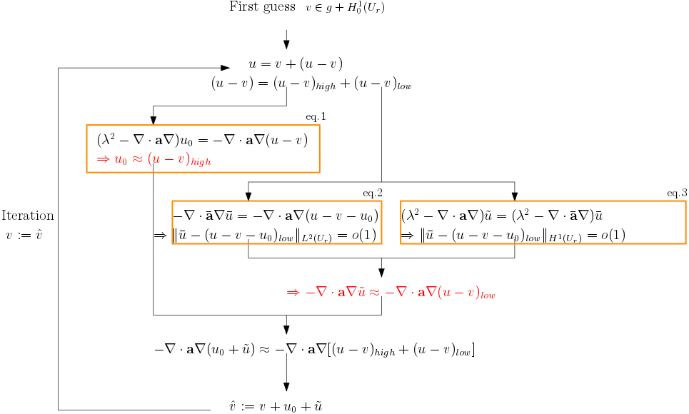
Figure 1: A flowchart shows the mechanic of the algorithm.

In this part, we explain heuristicly why the iterative algorthm converges to the true solution and how we figure out this algorithm. We keep in mind the main idea: To solve eq. 1.2, we divide it into sub-problems of regularized equations and homogenized equations.

We start with an initial guess of the solution $v$, then we write $u=v+(u-v)$ and we want to recover the part $(u-v)$. Since the divergence form is linear, we have

$$-\nabla\cdot\mathbf{a}\nabla(u-v)=-\nabla\cdot\mathbf{a}\nabla u+\nabla\cdot\mathbf{a}\nabla v=f+\nabla\cdot\mathbf{a}\nabla v.$$

In the first step of our algorithm, we solve the problem with regularization

$$(\lambda^{2}-\nabla\cdot\mathbf{a}\nabla)u_{0}=f+\nabla\cdot\mathbf{a}\nabla v,$$

and $u_{0}$ gives the high frequency part of $(u-v)$ associated to the operator $-\nabla\cdot\mathbf{a}\nabla$ on $U_{r}$. To see it, we apply the theorem of spectral decomposition [43, Chapter 5]

$$(u-v)=\sum_{i}^{\infty}\psi_{i},$$

where $\psi_{i}$ is the projection on the subspace of the eigenvalue $\kappa_{i}$ associated to $-\nabla\cdot\mathbf{a}\nabla$ on $U_{r}$, with $0<\kappa_{1}<\kappa_{2}\cdots$. Then $u_{0}$ has an expression

$$u_{0}=\sum_{i=1}^{\infty}\frac{\kappa_{i}}{\lambda^{2}+\kappa_{i}}\psi_{i}.$$

We see the projections associated to large eigenvalues have a small perturbation after the regularization. Thus, we consider the solution $u_{0}$ of the high frequency projection of $(u-v)$. Informally, we write

$$(u-v) \approx (u-v)_{high}+(u-v)_{low},$$

$$u_{0} = (u-v)_{high}.$$

Therefore, after the first step, we do not get all the information of $(u-v)$ but $(u-v)_{high}$ and the second and the third equation serve to recover $(u-v)_{low}$ of $(u-v)$. Using the superposition, a direct idea is to solve

$$-\nabla\cdot\mathbf{a}\nabla\widetilde{u}\approx-\nabla\cdot\mathbf{a}\nabla(u-v-u_{0})=\lambda^{2}u_{0}.$$ (1.11)

But for the reason of less numerical cost, we choose to solve at first a homogenized problem

$$-\nabla\cdot\bar{\mathbf{a}}\nabla\bar{u}=-\nabla\cdot\mathbf{a}\nabla(u-v-u_{0})=\lambda^{2}u_{0},$$ (1.12)

and if we believe that $-\nabla\cdot\mathbf{a}\nabla\widetilde{u}\approx-\nabla\cdot\bar{\mathbf{a}}\nabla\bar{u}$, we can also solve the one by adding regularization

$$(\lambda^{2}-\nabla\cdot\mathbf{a}\nabla)\widetilde{u}=(\lambda^{2}-\nabla\cdot\bar{\mathbf{a}}\nabla)\bar{u}.$$ (1.13)

Then, we hope that this $\widetilde{u}$ gives us $(u-v)_{low}$. Perhaps this "$\approx$" is not very precise, so we do $\hat{v}:=v+u_{0}+\widetilde{u}$ and put $\hat{v}$ in the role of $v$ for several iterations in order to get a further approach to the solution of eq. 1.2.

2 Notation

In this section, we state our assumptions about the coefficient field precisely and introduce some notations.

2.1 Assumptions on the coefficient field

We denote by $\left((\mathbf{a}(x))_{x\in\mathbb{R}^{d}},\mathcal{F},\operatorname{\mathbb{P}}\right)$ the probability space, and by $\mathcal{F}_{V}$ the $\sigma$-algebra generated by

$$\mathbf{a}\mapsto\int_{\mathbb{R}^{d}}\chi\mathbf{a}_{i,j},\text{ where }i,j\in\{1,2,3\cdots d\},\chi\in C^{\infty}_{c}(V).$$

$\mathcal{F}$ is short for $\mathcal{F}_{\mathbb{R}^{d}}$. $T_{y}$ denotes the operator of translation i.e. for any function $f$, $T_{y}(f)(x):=f(x+y)$ and for any set $A$, $T_{y}(A):=\{x+y|x\in A\}$.

The precise assumptions for the coefficient field are as follows.

1. $\mathbb{Z}^{d}$-stationarity: For each $A\in\mathcal{F}$ and each $y\in\mathbb{Z}^{d}$, we have $\operatorname{\mathbb{P}}[T_{y}(A)]=\operatorname{\mathbb{P}}[A]$.

2. Unit range correlation:

   $$\forall W,V\in\mathcal{B}(\mathbb{R}^{d}),\quad d_{H}(W,V)>1\implies\mathcal{F}_{W},\mathcal{F}_{V}\text{ are independent. }$$

   Here $d_{H}$ is the Hausdorff distance in $\mathbb{R}^{d}$.

3. Uniform ellipticity: There exists $0<\Lambda<\infty$ such that with probability one and for every $x,\xi\in\mathbb{R}^{d}$, we have $\Lambda^{-1}|\xi|^{2}\leqslant\xi\cdot\mathbf{a}(x)\xi\leqslant\Lambda|\xi|^{2}$.

2.2 Notation $\mathcal{O}_{s}$

We recall the definition of $\mathcal{O}_{s}$

$$X\leqslant\mathcal{O}_{s}(\theta)\iff\operatorname{\mathbb{E}}\left[\exp((\theta^{-1}X)_{+}^{s})\right]\leqslant 2,$$ (2.1)

where $(\theta^{-1}X)_{+}$ means $\max\{\theta^{-1}X,0\}$. This notation gives the tail estimate of random variables: One can use Markov’s inequality to obtain that

$$X\leqslant\mathcal{O}_{s}(\theta)\Longrightarrow\forall x>0,\operatorname{\mathbb{P}}[X\geqslant\theta x]\leqslant 2\exp(-x^{s}).$$

Moreover, we can also obtain the estimate of the sum of a series of random variables without its joint distribution: For a measure space $(E,\mathcal{S},m)$ and $\{X(z)\}_{z\in E}$ a family of random variables, we have

$$\forall z\in\mathcal{O}_{s}(E),X(z)\leqslant\mathcal{O}_{s}(\theta(z))\Longrightarrow\int_{E}X(z)m(dz)\leqslant\mathcal{O}_{s}\left(C_{s}\int_{E}\theta(z)m(dz)\right),$$ (2.2)

where $0<C_{s}<\infty$ is a constant and $C_{s}=1$ for $s\geqslant 1$. See Appendix of [6, Appendix A] for proofs and other operations on $\mathcal{O}_{s}$.

2.3 Convolution

For $f\in L^{p}(\mathbb{R}^{d}),g\in L^{q}(\mathbb{R}^{d})$ where $\frac{1}{p}+\frac{1}{q}=1$, we denote by $f\star g$ the convolution of the function $f,g$

$$f\star g(x)=\int_{\mathbb{R}^{d}}f(y)g(x-y)\,dy.$$

In this article, two mollifiers used are the heat kernel $\Phi_{r}(x)$, defined for $r>0$ and $x\in\mathbb{R}^{d}$ by

$$\Phi_{r}(x):=\frac{1}{(4\pi r^{2})^{d/2}}\exp\left(-\frac{x^{2}}{4r^{2}}\right),$$

and the bump function $\zeta\in C^{\infty}_{c}(\mathbb{R}^{d})$

$$\zeta(x):=c_{d}\exp\left(-\left(\frac{1}{4}-|x|^{2}\right)^{-1}\right)\mathbf{1}_{\{|x|<\frac{1}{2}\}},$$

where $c_{d}$ is the constant of normalization such that $\int_{\mathbb{R}^{d}}\zeta(x)dx=1$. Finally, we use the notation

$$\zeta_{\varepsilon}(x)=\frac{1}{\varepsilon^{d}}\zeta\left(\frac{x}{\varepsilon}\right),$$

as a mollifier in scale $\varepsilon>0$ and we have $\text{supp}(\zeta_{\varepsilon})\subset\overline{B_{\varepsilon/2}}$.

2.4 Function spaces

We use $\{e_{1},e_{2},\cdots e_{d}\}$ as the canonical basis of $\mathbb{R}^{d}$. For every Borel set $U\subset\mathbb{R}^{d}$, let $|U|$ be its Lebesgue measure. For each $p\in[1,+\infty]$, we denote by $L^{p}(U)$ the classical Lebesgue space and $L^{p}_{loc}(\mathbb{R}^{d})$ the function space for the functions with finite $L^{p}(V)$ norm for any compact set $V$. The weighted norm $\underline{L}^{p}(U)$ is defined for a bounded Borel set $U$ as

$$\|f\|_{\underline{L}^{p}(U)}=\left(\frac{1}{|U|}\int_{U}|f(x)|^{p}\,dx\right)^{\frac{1}{p}}=|U|^{-\frac{1}{p}}\|f\|_{L^{p}(U)}.$$

For each $k\in\mathbb{N}$, we denote by $H^{k}(U)$ the classical Sobolev space on $U$ equipped with the norm

$$\|f\|_{H^{k}(U)}:=\sum_{0\leqslant|\beta|\leqslant k}\|\partial^{\beta}f\|_{L^{2}(U)},$$

where $\beta\in\mathbb{N}^{d}$ represents a multi-index weak derivative,

$$|\beta|:=\sum_{i=1}^{d}\beta_{i}\quad\text{ and }\quad\partial^{\beta}f=\partial_{x_{1}}^{\beta_{1}}\cdots\partial_{x_{d}}^{\beta_{d}}f.$$

We also use $|\nabla^{k}f|$ to indicate $\sum_{|\beta|=k}|\partial^{\beta}f|$. When $|U|<\infty$, we define the weighted norm that

$$\|f\|_{\underline{H}^{k}(U)}:=\sum_{0\leqslant|\beta|\leqslant k}|U|^{\frac{|\beta|-k}{d}}\|\partial^{\beta}f\|_{\underline{L}^{2}(U)}.$$

$H^{k}_{0}(U)$ denotes the closure of $C_{c}^{\infty}(U)$ in $H^{k}(U)$ and $H^{-1}(U)$ for the dual of $H^{1}(U)$. The weighted norm $\underline{H}^{-1}(U)$ is

$$\|f\|_{\underline{H}^{-1}(U)}:=\sup\left\{\frac{1}{|U|}\int_{U}f(x)g(x)\,dx,g\in H^{1}_{0}(U),\|g\|_{\underline{H}^{1}(U)}\leqslant 1\right\}.$$

Here, we abuse the use of the integration $\int_{U}f(x)g(x)\,dx$, since the function space $H^{-1}(U)$ also contains linear functional, which is not necessarily a function.

Finally, we remark that one advantage of the definition of $\underline{H}^{k}$ is that it is consistent with the scale constant of Poincaré’s inequality [20, eq.(7.44)] and Sobolev extension theorem [20, Theorem 7.25]. That is, under the condition that the Borel set $U$ has $C^{1,1}$ boundary, for any function $f\in H^{1}_{0}(U_{r})$

$$\|f\|_{\underline{H}^{1}(U_{r})}\leqslant C(U,d)\|\nabla f\|_{\underline{L}^{2}(U_{r})},$$ (2.3)

and for any $f\in H^{2}(U_{r})$, there exists an extension $\operatorname{\mathsf{Ext}}(f)\in H_{0}^{2}(\mathbb{R}^{d})$ such that $\operatorname{\mathsf{Ext}}(f)\equiv f$ in $U_{r}$

$$\sum_{0\leqslant|\beta|\leqslant 2}|U_{r}|^{-\frac{d}{2}-\frac{|\beta|-2}{d}}\|\partial^{\beta}\operatorname{\mathsf{Ext}}(f)\|_{L^{2}(\mathbb{R}^{d})}\leqslant C(U,d)\|f\|_{\underline{H}^{2}(U_{r})}.$$ (2.4)

The proof depends on the scaling argument: For eq. 2.3, we prove at first the result in domain $U$ and then apply to $x\mapsto f(rx)$. For eq. 2.4, we apply [20, Theorem 7.25] to the domain $U$ and obtain an extension $\operatorname{\mathsf{Ext}}_{U}$ satisfying eq. 2.4 for $r=1$. Then, for the extension $\operatorname{\mathsf{Ext}}_{U_{r}}$ on the domain $U_{r}$, we define $\operatorname{\mathsf{Ext}}_{U_{r}}(f)(x):=\operatorname{\mathsf{Ext}}_{U}(f(r\cdot))(x/r)$ and this satisfies eq. 2.4 with a constant depending only on $U,d$. In the following paragraphs we neglect the index of domain and still note the extension $\operatorname{\mathsf{Ext}}$.

2.5 Cubes

We use the notation $\square$ to refer the open unit cube $\square:=\left(-\frac{1}{2},\frac{1}{2}\right)^{d}$. For any $z\in\mathbb{R}^{d}$, the translation of $\square$ in the direction $z$ writes $z+\square:=z+\left(-\frac{1}{2},\frac{1}{2}\right)^{d}$. The sum of a cube and a Borel set $U$ is defined as

$$\square+U:=\left\{z\in\mathbb{R}^{d}|z=x+y,x\in\square,y\in U\right\}.$$

We also denote define scaling of the cube by size $\varepsilon>0$ that $\square_{\varepsilon}:=\left(-\frac{\varepsilon}{2},\frac{\varepsilon}{2}\right)^{d}.$

3 Two technical lemmas

We prove two useful lemmas that improves the estimate of the iterative algorithm in this section. A formula similar to Lemma 3.1 can be found in [6, Lemme 6.7]. Here we introduce a variant version and it works well together with Lemma 3.2.

3.1 An inequality of localization

Lemma 3.1 (Mixed norm).

There exists a constant $0<C(d)<\infty$ such that for every $f\in L_{loc}^{2}(\mathbb{R}^{d})$, $g\in L^{2}(\mathbb{R}^{d})$ and every $\varepsilon>0,r\geqslant 2$, we have the following inequality

$$\|f(g\star\zeta_{\varepsilon})\|_{L^{2}(U_{r})}\leqslant C(d)\left(\max_{z\in\varepsilon\mathbb{Z}^{d}\cap(U_{r}+\square_{\varepsilon})}\|f\|_{\underline{L}^{2}(z+\square_{\varepsilon})}\right)\|g\|_{L^{2}(U_{r}+\square_{3\varepsilon})}.$$ (3.1)

Proof.

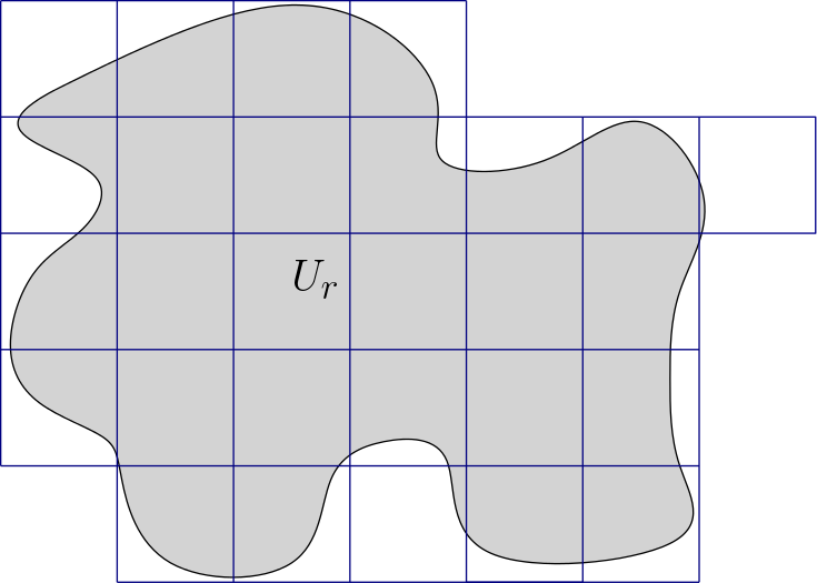
Figure 2: We calculate the $L^{2}$ norm by the sum of all norm in small cubes of size $\varepsilon$, so we counts all cubes in the domain $(U_{r}+\square_{\varepsilon})$.

We decompose the $L^{2}$ norm as the sum of that in small cubes $\square_{\varepsilon}$

$$\|f(g\star\zeta_{\varepsilon})\|^{2}_{L^{2}(U_{r})} \leqslant \sum_{z\in\varepsilon\mathbb{Z}^{d}\cap(U_{r}+\square_{\varepsilon})}\|f(g\star\zeta_{\varepsilon})\|^{2}_{L^{2}(z+\square_{\varepsilon})}$$

$$(\text{H\"{o}lder's inequality}) \leqslant \sum_{z\in\varepsilon\mathbb{Z}^{d}\cap(U_{r}+\square_{\varepsilon})}\left(\|f\|^{2}_{L^{2}(z+\square_{\varepsilon})}\|g\star\zeta_{\varepsilon}\|^{2}_{L^{\infty}(z+\square_{\varepsilon})}\right)$$

$$\leqslant \left(\max_{z\in\varepsilon\mathbb{Z}^{d}\cap(U_{r}+\square_{\varepsilon})}\|f\|^{2}_{L^{2}(z+\square_{\varepsilon})}\right)\left(\sum_{z\in\varepsilon\mathbb{Z}^{d}\cap(U_{r}+\square_{\varepsilon})}\|g\star\zeta_{\varepsilon}\|^{2}_{L^{\infty}(z+\square_{\varepsilon})}\right).$$

Noticing that for any $x\in z+\square_{\varepsilon},y\in B_{\varepsilon/2}$ then $(x-y)\in z+\square_{2\varepsilon}$ and we have

$$|g\star\zeta_{\varepsilon}(x)| = \left|\int_{\square_{\varepsilon}}g(x-y)\frac{1}{\varepsilon^{d}}\zeta(\frac{y}{\varepsilon})\,dy\right|$$

$$\leqslant \frac{C(d)}{\varepsilon^{d}}\int_{z+\square_{2\varepsilon}}|g(y)|\,dy$$

$$\leqslant \frac{C(d)}{\varepsilon^{d}}\left(\int_{z+\square_{2\varepsilon}}|g(y)|^{2}\,dy\right)^{\frac{1}{2}}|\square_{2\varepsilon}|^{\frac{1}{2}}$$

$$\leqslant \frac{C(d)}{\varepsilon^{\frac{d}{2}}}\|g\|_{L^{2}(z+\square_{2\varepsilon})}.$$

So we get

$$\|g\star\zeta_{\varepsilon}\|_{L^{\infty}(z+\square_{\varepsilon})}\leqslant\frac{C(d)}{\varepsilon^{\frac{d}{2}}}\|g\|_{L^{2}(z+\square_{2\varepsilon})},$$

and we add this analysis in the former inequality and obtain that

$$\|f(g\star\zeta_{\varepsilon})\|^{2}_{L^{2}(U_{r})} \leqslant C(d)\left(\frac{1}{\varepsilon^{d}}\max_{z\in\varepsilon\mathbb{Z}^{d}\cap(U_{r}+\square_{\varepsilon})}\|f\|^{2}_{L^{2}(z+\square_{\varepsilon})}\right)\left(\sum_{z\in\varepsilon\mathbb{Z}^{d}\cap(U_{r}+\square_{\varepsilon})}\|g\|^{2}_{L^{2}(z+\square_{2\varepsilon})}\right)$$

$$\leqslant C(d)\left(\max_{z\in\varepsilon\mathbb{Z}^{d}\cap(U_{r}+\square_{\varepsilon})}\|f\|^{2}_{\underline{L}^{2}(z+\square_{\varepsilon})}\right)\|g\|^{2}_{L^{2}(U_{r}+\square_{3\varepsilon})}.$$

This is the desired inequality. ∎

3.2 Maximum of finite number of random variables of type $\mathcal{O}_{s}(1)$

Since $\left(\max_{z\in\varepsilon\mathbb{Z}^{d}\cap(U_{r}+\square_{\varepsilon})}\|f\|_{\underline{L}^{2}(z+\square_{\varepsilon})}\right)$ often appears in the context as the maximum of a family of random variables, we prove the following lemma to analyze the maximum of a finite number of random variables of type $\mathcal{O}_{s}(1)$. Note that we do not make any assumptions on the joint law of the random variables.

Lemma 3.2.

For all $N\geqslant 1$ and a family of random variables $\{X_{i}\}_{1\leqslant i\leqslant N}$ satisfying that $X_{i}\leqslant\mathcal{O}_{s}(1)$, we have

$$\left(\max_{1\leqslant i\leqslant N}X_{i}\right)\leqslant\mathcal{O}_{s}\left(\left(\frac{\log(2N)}{\log(4/3)}\right)^{\frac{1}{s}}\right).$$ (3.2)

Proof.

For the case $N=1$, we could check that eq. 3.2 is established since

$$M=X_{1}\leqslant\mathcal{O}_{s}(1)\Longrightarrow M\leqslant\mathcal{O}_{s}\left(\frac{\log(4)}{\log(4/3)}\right),$$

so we focus on the case $N\geqslant 2$. By Markov’s inequality, $X_{i}\leqslant\mathcal{O}_{s}(1)$ gives us $\operatorname{\mathbb{P}}[X_{i}>x]\leqslant 2e^{-x^{s}}.$ Then we use the union bound to get

$$\operatorname{\mathbb{P}}\left[\max_{1\leqslant i\leqslant N}X_{i}>x\right]=\operatorname{\mathbb{P}}\left[\bigcup_{i=1}^{N}\{X_{i}>x\}\right]\leqslant\left(1\wedge\sum_{i=1}^{N}\operatorname{\mathbb{P}}[X_{i}>x]\right)\leqslant 1\wedge 2Ne^{-x^{s}}.$$ (3.3)

We denote by $x_{0}$ the critical point such that $e^{x_{0}^{s}}=2N$ and $a>0$ such that $a^{s}>3$ and its value will be chosen carefully later. We also set $M=\max_{1\leqslant i\leqslant N}X_{i}$ and use Fubini’s theorem: For an increasing positive function $g\in C^{1}(\mathbb{R})$ such that $g(0)=0$, we have

$$\operatorname{\mathbb{E}}\left[g(M)\right]=\int_{0}^{\infty}g(t)\operatorname{\mathbb{P}}[M>t]\,dt.$$ (3.4)

We apply eq. 3.4 the function $x\mapsto\exp\left(\left(\frac{x}{a}\right)_{+}^{s}\right)-1$,

$$\begin{split}\operatorname{\mathbb{E}}\left[\exp\left(\left(\frac{M}{a}\right)_{+}^{s}\right)\right]&=\int_{0}^{\infty}\frac{s}{a}\left(\frac{x}{a}\right)^{s-1}e^{(\frac{x}{a})^{s}}\operatorname{\mathbb{P}}[M>x]\,dx+1\\ &=\int_{0}^{x_{0}}\frac{s}{a}\left(\frac{x}{a}\right)^{s-1}e^{(\frac{x}{a})^{s}}\operatorname{\mathbb{P}}[M>x]\,dx\\ &\quad+\int_{x_{0}}^{\infty}\frac{s}{a}\left(\frac{x}{a}\right)^{s-1}e^{(\frac{x}{a})^{s}}\operatorname{\mathbb{P}}[M>x]\,dx+1.\end{split}$$ (3.5)

For the integration on the interval $(0,x_{0}]$, we use the estimate eq. 3.3 that $\operatorname{\mathbb{P}}[M>x]\leqslant 1$ and $e^{x_{0}^{s}}=2N$ to bound it

$$\begin{split}\int_{0}^{x_{0}}\frac{s}{a}\left(\frac{x}{a}\right)^{s-1}e^{(\frac{x}{a})^{s}}\operatorname{\mathbb{P}}[M>x]\,dx&\leqslant\int_{0}^{x_{0}}\frac{s}{a}\left(\frac{x}{a}\right)^{s-1}e^{(\frac{x}{a})^{s}}\,dx\\ &=\int_{0}^{x_{0}}e^{(\frac{x}{a})^{s}}\,d\left(\frac{x}{a}\right)^{s}\\ &=(2N)^{\frac{1}{a^{s}}}-1.\end{split}$$ (3.6)

Similarly, for the integration on the interval $(x_{0},\infty)$, we use eq. 3.3 to control the probability that $\operatorname{\mathbb{P}}[M>x]\leqslant 2Ne^{-x^{s}}$ and give an estimate

$$\begin{split}\int_{x_{0}}^{\infty}\frac{s}{a}\left(\frac{x}{a}\right)^{s-1}e^{(\frac{x}{a})^{s}}\operatorname{\mathbb{P}}[M>x]\,dx&\leqslant 2N\int_{x_{0}}^{\infty}\frac{s}{a}\left(\frac{x}{a}\right)^{s-1}e^{(\frac{x}{a})^{s}-x^{s}}\,dx\\ &=2N\int_{x_{0}}^{\infty}e^{(\frac{x}{a})^{s}-x^{s}}\,d\left(\frac{x}{a}\right)^{s}\\ &=\underbrace{\frac{1}{a^{s}-1}}_{\text{Using }a^{s}\geqslant 3}(2N)^{\frac{1}{a^{s}}}\\ &\leqslant\frac{1}{2}(2N)^{\frac{1}{a^{s}}}.\\ \end{split}$$ (3.7)

Now we fix $a=\left(\frac{\log(2N)}{\log(4/3)}\right)^{\frac{1}{s}}$. For the case $N\geqslant 2$, we can check that

$$a^{s}=\left(\frac{\log(2N)}{\log(4/3)}\right)\geqslant\left(\frac{\log(4)}{\log(4/3)}\right)>3,$$

so $a^{s}\geqslant 3$ is satisfied. Finally, we put back the estimate eq. 3.6 and eq. 3.7 back to eq. 3.5 and verify the definition of $\mathcal{O}_{s}$

$$\operatorname{\mathbb{E}}\left[\exp\left(\left(\frac{M}{a}\right)_{+}^{s}\right)\right]\leqslant\frac{3}{2}(2N)^{\frac{1}{a^{s}}}=\frac{3}{2}e^{\log(4/3)}=2.$$

This finishes the proof. ∎

4 Two-scale expansion estimate

This section reformulates [3, Theorem 3.1] a quantitative two-scale expansion theorem with the improvements from the lemmas in Section 3.

4.1 Main structure

The two-scale expansion allows us to approximate the solution of eq. 1.2 by the solution of the homogenized equation and the first order corrector $\{\phi_{e_{k}}\}_{1\leqslant k\leqslant d}$. We recall at first the definition of the first order corrector.

Definition 4.1 (First order corrector, Lemma 3.16 and Theorem 4.1 of [6]).

For each $p\in\mathbb{R}^{d}$, the corrector $\phi_{p}$ is the sublinear function satisfying that $p\cdot x+\phi_{p}$ is $\mathbf{a}$-harmonic in whole space $\mathbb{R}^{d}$ i.e.

$$-\nabla\cdot\mathbf{a}(p+\nabla\phi_{p})=0,\text{ in }\mathbb{R}^{d}.$$ (4.1)

$\nabla\phi_{p}$ is $\mathbb{Z}^{d}$-stationary and $\phi_{p}$ is well-defined up to a constant. For $d\geqslant 3$, we can choose a constant such that $\operatorname{\mathbb{E}}\left[\int_{\square}\phi_{p}\right]=0$, and in this case $\phi_{p}$ is also $\mathbb{Z}^{d}$-stationary.

We remark that proof of the property $\phi_{p}$ is $\mathbb{Z}^{d}$-stationary for $d\geqslant 3$ requires a detailed quantitative study of the following modified corrector

$$\phi^{(\lambda)}_{p}:=\phi_{p}-\phi_{p}\star\Phi_{\lambda^{-1}},$$ (4.2)

which is $\mathbb{Z}^{d}$-stationary and is always well-defined. Then the quantitative study of $\phi^{(\lambda)}_{p}$ allows us to extract a limit in the subsequence when $\lambda\rightarrow 0$ and this gives us a candidate for the choice of constant. For its complete proof, see [6, Chapter 4.6, Page 175]. In the following paragraphs, we specify the constant by $\operatorname{\mathbb{E}}\left[\int_{\square}\phi_{p}\right]=0$. Therefore, we can use the property that $\phi_{p}$ is $\mathbb{Z}^{d}$-stationary for $d\geqslant 3$.

Once we define the first-order corrctor, as well-known from [1], for $v$ the heterogeneous and $\bar{v}$ the homogenized solution, the two-scale expansion $\bar{v}+\sum_{k=1}^{d}(\partial_{x_{k}}\bar{v})\phi_{e_{k}}$ approximates $v$ in the sense $H^{1}$. We follow the similar idea in [6, Chapter 6] and apply a modified two-scale expansion to $\bar{v}\in H^{1}_{0}(U_{r})\cap H^{2}(U_{r})$ with $\{\phi^{(\lambda)}_{e_{k}}\}_{1\leqslant k\leqslant d}$ defind in eq. 4.2

$$w:=\bar{v}+\sum_{k=1}^{d}\partial_{x_{k}}(\operatorname{\mathsf{Ext}}(\bar{v})\star\zeta)\phi^{(\lambda)}_{e_{k}},$$ (4.3)

where $\operatorname{\mathsf{Ext}}(\bar{v})$ is the Sobolev extension such that eq. 2.4 is established. In the following we abuse a little the notation to identify

$$\bar{v}\star\zeta:=\operatorname{\mathsf{Ext}}(\bar{v})\star\zeta,$$ (4.4)

in order to shorter the equation. We want to prove a $H^{1}$ convergence theorem for the operator $(\mu^{2}-\nabla\cdot\mathbf{a}\nabla)$. We also recall the definition of $\ell(\lambda)$

$$\ell(\lambda)=\left\{\begin{array}[]{ll}(\log(1+\lambda^{-1}))^{\frac{1}{2}}&d=2,\\ 1&d>2.\end{array}\right.$$

Theorem 4.1 (Two-scale estimate).

For every $r\geqslant 2,\lambda\in(\frac{1}{r},\frac{1}{2})$, there exists three $\mathcal{F}$-measurable random variables $\mathcal{X}_{1},\mathcal{X}_{2},\mathcal{Y}_{1}$ satisfying for each $s\in(0,2)$, there exists a constant $C^{\prime}(U,s,d)$ such that the following holds: $\mathcal{X}_{1},\mathcal{X}_{2},\mathcal{Y}_{1}$ have an estimate

$$\mathcal{X}_{1}\leqslant\mathcal{O}_{s}\left(C^{\prime}(U,s,d)\ell(\lambda)(\log r)^{\frac{1}{s}}\right), \mathcal{X}_{2}\leqslant\mathcal{O}_{s}\left(C^{\prime}(U,s,d)\lambda^{\frac{d}{2}}(\log r)^{\frac{1}{s}}\right),$$ (4.5)

$$\mathcal{Y}_{1}\leqslant\mathcal{O}_{s}\left(C^{\prime}(U,s,d)\ell(\lambda)(\log r)^{\frac{1}{s}}\right),$$ (4.6)

and for every $\bar{v}\in H^{1}_{0}(U_{r})\cap H^{2}(U_{r}),\mu\in[0,\lambda]$ and $v\in H^{1}_{0}(U_{r})$ satisfying

$$(\mu^{2}-\nabla\cdot a\nabla)v=(\mu^{2}-\nabla\cdot\bar{\mathbf{a}}\nabla)\bar{v}\qquad\text{ in }U_{r},$$ (4.7)

we have an $H^{1}$ estimate for the two-scale expansion $w$ associated to $\bar{v}$ defined in eq. 4.3

$$\begin{split}\|v-w\|_{\underline{H}^{1}(U_{r})}&\leqslant C(U,\Lambda,d)\left[\vphantom{\frac{1}{2}}\|\bar{v}\|_{\underline{H}^{2}(U_{r})}+\left(\|\bar{v}\|_{\underline{H}^{2}(U_{r})}+\mu\|\bar{v}\|_{\underline{H}^{1}(U_{r})}\right)\mathcal{X}_{1}\right.\\ &\qquad\left.+\left(\ell(\lambda)^{\frac{1}{2}}\|\bar{v}\|^{\frac{1}{2}}_{\underline{H}^{2}(U_{r})}\|\bar{v}\|^{\frac{1}{2}}_{\underline{H}^{1}(U_{r})}+\|\bar{v}\|_{\underline{H}^{1}(U_{r})}\right)\mathcal{X}_{2}\right.\\ &\qquad\left.+\left(\ell(\lambda)^{\frac{1}{2}}\left(\mu+\frac{1}{r}+\frac{1}{\ell(\lambda)}\right)\|\bar{v}\|^{\frac{1}{2}}_{\underline{H}^{2}(U_{r})}\|\bar{v}\|^{\frac{1}{2}}_{\underline{H}^{1}(U_{r})}+\|\bar{v}\|_{\underline{H}^{2}(U_{r})}\right)\mathcal{Y}_{1}\right].\\ \end{split}$$ (4.8)

Remark.

The explicit expression of $\mathcal{X}_{1},\mathcal{X}_{2},\mathcal{Y}_{1}$ can be checked in fig. 3. They are the maximum of local spatial average of gradient and the flux of the first order corrector.

Proof.

We give at first the proof of the deterministic part. We will see that the errors can finally be reduced to the estimates of two norms: the interior error term and a boundary layer term. The latter boundary term comes from the fact that $v$ and $w$ do not have the same boundary condition. So we introduce $b$ the solution of the equation

$$\left\{\begin{array}[]{ll}(\mu^{2}-\nabla\cdot\mathbf{a}\nabla)b=0&\text{ in }U_{r},\\ b=\sum_{k=1}^{d}\partial_{x_{k}}(\bar{v}\star\zeta)\phi^{(\lambda)}_{e_{k}}&\text{ on }\partial U_{r}.\end{array}\right.$$ (4.9)

Then $(w-b)$ shares the same boundary condition as $v$. So, we have

$$\|v-w\|_{\underline{H}^{1}(U_{r})}\leqslant\|v+b-w\|_{\underline{H}^{1}(U_{r})}+\|b\|_{\underline{H}^{1}(U_{r})},$$ (4.10)

and we do estimates of the two parts respectively.

• Estimate for $(v+b-w)$. We denote by $z:=v+b-w\in H^{1}_{0}(U_{r})$ and test it in eq. 4.7 and eq. 4.9

  $$\mu^{2}\int_{U_{r}}zv+\int_{U_{r}}\nabla z\cdot\mathbf{a}\nabla v = \mu^{2}\int_{U_{r}}z\bar{v}+\int_{U_{r}}\nabla z\cdot\bar{\mathbf{a}}\nabla\bar{v},$$

  $$\mu^{2}\int_{U_{r}}zb+\int_{U_{r}}\nabla z\cdot\mathbf{a}\nabla b = 0.$$

  We do the sum to obtain that

  $$\mu^{2}\int_{U_{r}}z(v+b)+\int_{U_{r}}\nabla z\cdot\mathbf{a}\nabla(v+b)=\mu^{2}\int_{U_{r}}z\bar{v}+\int_{U_{r}}\nabla z\cdot\bar{\mathbf{a}}\nabla\bar{v}.$$

  Using the fact $v+b=z+w$, we obtain

  $$\mu^{2}\int_{U_{r}}|z|^{2}+\int_{U_{r}}\nabla z\cdot\mathbf{a}\nabla z=\mu^{2}\int_{U_{r}}z(\bar{v}-w)+\int_{U_{r}}\nabla z\cdot(\bar{\mathbf{a}}\nabla\bar{v}-\mathbf{a}\nabla w),$$

  and we apply the uniform ellipticity condition to obtain

  $$\mu^{2}\|z\|^{2}_{\underline{L}^{2}(U_{r})}+\Lambda^{-1}\|\nabla z\|^{2}_{\underline{L}^{2}(U_{r})} \leqslant \mu^{2}\|z\|_{\underline{L}^{2}(U_{r})}\|w-\bar{v}\|_{\underline{L}^{2}(U_{r})}$$

  $$+\|z\|_{\underline{H}^{1}(U_{r})}\|\nabla\cdot\mathbf{a}\nabla w-\nabla\cdot\bar{\mathbf{a}}\nabla\bar{v}\|_{\underline{H}^{-1}(U_{r})}$$

  $$(\text{Young's inequality}) \leqslant \mu^{2}\|z\|^{2}_{\underline{L}^{2}(U_{r})}+\frac{\mu^{2}}{4}\|w-\bar{v}\|^{2}_{\underline{L}^{2}(U_{r})}$$

  $$+\frac{\Lambda^{-1}}{2}\|z\|^{2}_{\underline{H}^{1}(U_{r})}+\frac{\Lambda}{2}\|\nabla\cdot\mathbf{a}\nabla w-\nabla\cdot\bar{\mathbf{a}}\nabla\bar{v}\|^{2}_{\underline{H}^{-1}(U_{r})}$$

  $$\Longrightarrow\|\nabla z\|_{\underline{L}^{2}(U_{r})} \leqslant \Lambda\|\nabla\cdot\mathbf{a}\nabla w-\nabla\cdot\bar{\mathbf{a}}\nabla\bar{v}\|_{\underline{H}^{-1}(U_{r})}+\sqrt{\Lambda}\mu\|w-\bar{v}\|_{\underline{L}^{2}(U_{r})}.$$

  We use Poincaré’s inequality to conclude that

  $$\|z\|_{\underline{H}^{1}(U_{r})}\leqslant C(U)\left(\Lambda\|\nabla\cdot\mathbf{a}\nabla w-\nabla\cdot\bar{\mathbf{a}}\nabla\bar{v}\|_{\underline{H}^{-1}(U_{r})}+\sqrt{\Lambda}\mu\|w-\bar{v}\|_{\underline{L}^{2}(U_{r})}\right).$$ (4.11)

• Estimate for $b$. To estimate $b$ we use the property that it is the optimizer of the problem

  $$\inf_{\chi\in b+H^{1}_{0}(U_{r})}\mu^{2}\int_{U_{r}}\chi^{2}+\int_{U_{r}}\nabla\chi\cdot\mathbf{a}\nabla\chi.$$

  So we give an upper bound of this functional by the following trial function

  $$T_{\lambda}:=\left(\mathbf{1}_{\mathbb{R}^{d}\backslash U_{r,2\ell(\lambda)}}\star\zeta_{\ell(\lambda)}\right)\sum_{k=1}^{d}\partial_{x_{k}}(\bar{v}\star\zeta)\phi^{(\lambda)}_{e_{k}},$$ (4.12)

  where $U_{r,2\ell(\lambda)}$ is defined as

  $$U_{r,2\ell(\lambda)}=\{x\in U_{r}|d(x,\partial U_{r})>2\ell(\lambda)\}.$$

  The motivation to test $T_{\lambda}$ is the following: If we think the solution of elliptic equation is an average in some sense of the boundary value, then when the coefficient is oscillating, the boundary value is hard to propagate. So one naive candidate is just smoothing the boundary value in a small band of length $2\ell(\lambda)$.

  By comparison,

  $$\mu^{2}\int_{U_{r}}|b|^{2}+\int_{U_{r}}\nabla b\cdot\mathbf{a}\nabla b \leqslant \mu^{2}\int_{U_{r}}|T_{\lambda}|^{2}+\int_{U_{r}}\nabla T_{\lambda}\cdot\mathbf{a}\nabla T_{\lambda}$$

  $$\Longrightarrow\|\nabla b\|_{\underline{L}^{2}(U_{r})} \leqslant \mu\sqrt{\Lambda}\|T_{\lambda}\|_{\underline{L}^{2}(U_{r})}+\Lambda\|\nabla T_{\lambda}\|_{\underline{L}^{2}(U_{r})}.$$

  Moreover, to estimate the $L^{2}$ norm, we use once again Poincaré’s inequality

  $$\|b\|_{\underline{L}^{2}(U_{r})} = \|b-T_{\lambda}+T_{\lambda}\|_{\underline{L}^{2}(U_{r})}$$

  $$\leqslant \|b-T_{\lambda}\|_{\underline{L}^{2}(U_{r})}+\|T_{\lambda}\|_{\underline{L}^{2}(U_{r})}$$

  (Poincaré’s inequality) $$\leqslant r\|\nabla(b-T_{\lambda})\|_{\underline{L}^{2}(U_{r})}+\|T_{\lambda}\|_{\underline{L}^{2}(U_{r})}$$

  $$\leqslant r\|\nabla b\|_{\underline{L}^{2}(U_{r})}+r\|\nabla T_{\lambda}\|_{\underline{L}^{2}(U_{r})}+\|T_{\lambda}\|_{\underline{L}^{2}(U_{r})}.$$

  We combine the two and get an estimate of $b$

  $$\|b\|_{\underline{H}^{1}(U_{r})} = \frac{1}{|U_{r}|^{\frac{1}{d}}}\|b\|_{\underline{L}^{2}(U_{r})}+\|\nabla b\|_{\underline{L}^{2}(U_{r})}$$

  $$\leqslant C(U)\left(\frac{1}{r}\|T_{\lambda}\|_{\underline{L}^{2}(U_{r})}+\mu\sqrt{\Lambda}\|T_{\lambda}\|_{\underline{L}^{2}(U_{r})}+(1+\Lambda)\|\nabla T_{\lambda}\|_{\underline{L}^{2}(U_{r})}\right).$$

Finally, we put all the estimates above into eq. 4.10

$$\begin{split}\|v-w\|_{\underline{H}^{1}(U_{r})}&\leqslant C(U,\Lambda)\left(\vphantom{\frac{1}{2}}\|\nabla\cdot(\mathbf{a}\nabla w-\bar{\mathbf{a}}\nabla\bar{v})\|_{\underline{H}^{-1}(U_{r})}+\mu\|w-\bar{v}\|_{\underline{L}^{2}(U_{r})}\right.\\ &\qquad\qquad\qquad\left.+\|\nabla T_{\lambda}\|_{\underline{L}^{2}(U_{r})}+\left(\frac{1}{r}+\mu\right)\|T_{\lambda}\|_{\underline{L}^{2}(U_{r})}\right).\end{split}$$ (4.13)

To complete the proof of Theorem 4.1, we have to treat the random norms in eq. 4.13 respectively. It is the main task of the next section. ∎

4.2 Construction of a vector field

In this part, we analyze $\|\nabla\cdot(\mathbf{a}\nabla w-\bar{\mathbf{a}}\nabla\bar{v})\|_{\underline{H}^{-1}(U_{r})}$ with the help of the flux corrector. Similar formulas appear both in [3, Lemma 3.3] and [6, Chapter 6, Lemma 6.7], here we give the version in our context.

At first, we introduce the flux corrector $\mathbf{S}_{p}$. For every $p\in\mathbb{R}^{d}$, since $\mathbf{g}_{p}:=\mathbf{a}(p+\nabla\phi_{p})-\bar{\mathbf{a}}p$ defines a divergence free field, i.e. $\nabla\cdot\mathbf{g}_{p}=0$, it admits a representation as the "curl" of some potential vector by Helmholtz’s theorem. That is there exists a $\mathbb{R}^{d\times d}$ skew-symmetric matrix $\mathbf{S}_{p}$ such that

$$\mathbf{a}(p+\nabla\phi_{p})-\bar{\mathbf{a}}p=\nabla\cdot\mathbf{S}_{p},$$

where $\nabla\cdot\mathbf{S}_{p}$ is a $\mathbb{R}^{d}$ valued vector defined by $(\nabla\cdot\mathbf{S}_{p})_{i}=\sum_{j=1}^{d}\partial_{x_{j}}\mathbf{S}_{p,ij}$. In order to "fix the gauge", for each $i,j\in\{1,2,\cdots d\}$, we force

$$\Delta\mathbf{S}_{p,ij}=\partial_{x_{j}}\mathbf{g}_{p,i}-\partial_{x_{i}}\mathbf{g}_{p,j},$$

and under this condition, $\mathbf{S}_{p}$ is unique up to a constant and $\{\nabla\mathbf{S}_{p},ij,p\in\mathbb{R}^{d},i,j\in\{1,2,\cdots d\}\}$ also forms a family of $\mathbb{Z}^{d}$-stationary field like $\nabla\phi_{p}$. This quantity appears in the early work of periodic homogenization [9, Lemma 3.1] and [32, Lemma 4.4]. See [6, Lemma 6.1] for the well-definedness of $\mathbf{S}_{p}$ in stochatic homogenization setting and this quantity is also adapted in [24, Lemma 1] as extended corrector. We also define

$$\mathbf{S}_{p}^{(\lambda)}=\mathbf{S}_{p}-\mathbf{S}_{p}\star\Phi_{\lambda^{-1}},$$

to truncate the constant part, so $\mathbf{S}_{p}^{(\lambda)}$ is well-defined and $\mathbb{Z}^{d}$-stationary.

We have the following identity.

Lemma 4.1.

For $\lambda>0,\bar{v}\in H_{0}^{1}(U_{r})\cap H^{2}(U_{r})$ and $w\in H^{1}(U_{r})$ as in Theorem 4.1. We construct a vector field $\mathbf{F}$ such that

$$\nabla\cdot(\mathbf{a}\nabla w-\bar{\mathbf{a}}\nabla\bar{v})=\nabla\cdot\mathbf{F},$$

whose i-th component is given by

$$\begin{split}\mathbf{F}_{i}&=\sum_{j=1}^{d}(\mathbf{a}_{ij}-\bar{\mathbf{a}}_{ij})\partial_{x_{j}}(\bar{v}-\bar{v}\star\zeta)+\sum_{j,k=1}^{d}\left(\mathbf{a}_{ij}\phi^{(\lambda)}_{e_{k}}-\mathbf{S}^{(\lambda)}_{e_{k},ij}\right)\partial_{x_{j}}\partial_{x_{k}}(\bar{v}\star\zeta)\\ &\qquad+\sum_{j,k=1}^{d}\left(\partial_{x_{j}}\mathbf{S}_{e_{k},ij}\star\Phi_{\lambda^{-1}}-\mathbf{a}_{ij}\partial_{x_{j}}\phi_{e_{k}}\star\Phi_{\lambda^{-1}}\right)\partial_{x_{k}}(\bar{v}\star\zeta).\end{split}$$ (4.14)

Proof.

We develop

$$\left[\mathbf{a}\nabla w-\bar{\mathbf{a}}\nabla\bar{v}\right]_{i} = \left[\mathbf{a}\nabla\left(\bar{v}+\sum_{k=1}^{d}\partial_{x_{k}}(\bar{v}\star\zeta)\phi^{(\lambda)}_{e_{k}}\right)-\bar{\mathbf{a}}\nabla\bar{v}\right]_{i}$$

$$= \left[(\mathbf{a}-\bar{\mathbf{a}})\nabla\bar{v}+\mathbf{a}\nabla\sum_{k=1}^{d}\left(\partial_{x_{k}}(\bar{v}\star\zeta)\phi^{(\lambda)}_{e_{k}}\right)\right]_{i}$$

$$= \underbrace{\left[(\mathbf{a}-\bar{\mathbf{a}})\nabla(\bar{v}-\bar{v}\star\zeta)\right]_{i}}_{\mathbf{I}}+\underbrace{\left[(\mathbf{a}-\bar{\mathbf{a}})\nabla(\bar{v}\star\zeta)+\mathbf{a}\nabla\sum_{k=1}^{d}\left(\partial_{x_{k}}(\bar{v}\star\zeta)\phi^{(\lambda)}_{e_{k}}\right)\right]_{i}}_{\mathbf{II}}.$$

The first term is indeed

$$\mathbf{I}=\left[(\mathbf{a}-\bar{\mathbf{a}})\nabla(\bar{v}-\bar{v}\star\zeta)\right]_{i}=\sum_{j=1}^{d}(\mathbf{a}_{ij}-\bar{\mathbf{a}}_{ij})\partial_{x_{j}}(\bar{v}-\bar{v}\star\zeta),$$

as in the right hand side of the identity, so we continue to study the rest of the formula.

$$\mathbf{II} = \sum_{j=1}^{d}(\mathbf{a}_{ij}-\bar{\mathbf{a}}_{ij})\partial_{x_{j}}(\bar{v}\star\zeta)+\sum_{j,k=1}^{d}\mathbf{a}_{ij}\partial_{x_{j}}\left(\partial_{x_{k}}(\bar{v}\star\zeta)\phi^{(\lambda)}_{e_{k}}\right)$$

$$= \sum_{j,k=1}^{d}(\mathbf{a}_{ij}-\bar{\mathbf{a}}_{ij})\partial_{x_{j}}(\bar{v}\star\zeta)\delta_{jk}+\sum_{j,k=1}^{d}\mathbf{a}_{ij}\partial_{x_{j}}\partial_{x_{k}}(\bar{v}\star\zeta)\phi^{(\lambda)}_{e_{k}}+\sum_{j,k=1}^{d}\mathbf{a}_{ij}\partial_{x_{k}}(\bar{v}\star\zeta)\partial_{x_{j}}\phi^{(\lambda)}_{e_{k}}$$

$$= \underbrace{\sum_{j,k=1}^{d}\left((\mathbf{a}_{ij}-\bar{\mathbf{a}}_{ij})\delta_{jk}+\mathbf{a}_{ij}\partial_{x_{j}}\phi^{(\lambda)}_{e_{k}}\right)\partial_{x_{k}}(\bar{v}\star\zeta)}_{\mathbf{II.1}}+\underbrace{\sum_{j,k=1}^{d}\mathbf{a}_{ij}\partial_{x_{j}}\partial_{x_{k}}(\bar{v}\star\zeta)\phi^{(\lambda)}_{e_{k}}}_{\mathbf{II.2}}.$$

$\mathbf{II.2}$ appears in the right hand side of the formula, so it remains $\mathbf{II.1}$ to treat. We use the the definition of $\mathbf{S}_{e_{k}}^{(\lambda)}$ in $\mathbf{II.1}$

$$\mathbf{II.1} = \sum_{k=1}^{d}\left[\mathbf{a}(e_{k}+\nabla\phi^{(\lambda)}_{e_{k}})-\bar{\mathbf{a}}e_{k}\right]_{i}\partial_{x_{k}}(\bar{v}\star\zeta)$$

$$= \sum_{k=1}^{d}\left[\mathbf{a}(e_{k}+\nabla\phi_{e_{k}})-\bar{\mathbf{a}}e_{k}-\mathbf{a}\nabla\phi_{e_{k}}\star\Phi_{\lambda^{-1}}\right]_{i}\partial_{x_{k}}(\bar{v}\star\zeta)$$

$$= \sum_{k=1}^{d}\left[\nabla\cdot\mathbf{S}_{e_{k}}-\mathbf{a}\nabla\phi_{e_{k}}\star\Phi_{\lambda^{-1}}\right]_{i}\partial_{x_{k}}(\bar{v}\star\zeta)$$

$$= \underbrace{\sum_{k=1}^{d}\left[\nabla\cdot\mathbf{S}^{(\lambda)}_{e_{k}}\right]_{i}\partial_{x_{k}}(\bar{v}\star\zeta)}_{\mathbf{III}}+\sum_{k=1}^{d}\left[\nabla\cdot\mathbf{S}_{e_{k}}\star\Phi_{\lambda^{-1}}-\mathbf{a}\nabla\phi_{e_{k}}\star\Phi_{\lambda^{-1}}\right]_{i}\partial_{x_{k}}(\bar{v}\star\zeta).$$

All the terms match well except $\mathbf{III}$, where we have to look for an equal form after divergence. Thanks to the property of skew-symmetry, we have

$$\nabla\cdot\mathbf{III} = \nabla\cdot\left(\sum_{k=1}^{d}\left[\nabla\cdot\mathbf{S}^{(\lambda)}_{e_{k}}\right]_{i}\partial_{x_{k}}(\bar{v}\star\zeta)\right)$$

$$= \sum_{i,j,k=1}^{d}\partial_{x_{i}}\left(\partial_{x_{j}}\mathbf{S}^{(\lambda)}_{e_{k},ij}\,\partial_{x_{k}}(\bar{v}\star\zeta)\right)$$

$$(\text{Integration by parts}) = \sum_{i,j,k=1}^{d}\partial_{x_{i}}\partial_{x_{j}}\left(\mathbf{S}^{(\lambda)}_{e_{k},ij}\partial_{x_{k}}(\bar{v}\star\zeta)\right)-\partial_{x_{i}}\left(\mathbf{S}^{(\lambda)}_{e_{k},ij}\,\partial_{x_{j}}\partial_{x_{k}}(\bar{v}\star\zeta)\right)$$

$$(\text{Skew-symmetry of }\mathbf{S}) = -\nabla\cdot\left(\sum_{j,k=1}^{d}\mathbf{S}^{(\lambda)}_{e_{k},ij}\,\partial_{x_{j}}\partial_{x_{k}}(\bar{v}\star\zeta)\right).$$

This finishes the proof. ∎

4.3 Quantitative description of $\phi^{(\lambda)}_{e_{k}}$ and $\mathbf{S}^{(\lambda)}_{e_{k}}$

In this subsection, we will give some quantitative descriptions of $\phi^{(\lambda)}_{e_{k}}$ and $\mathbf{S}^{(\lambda)}_{e_{k}}$, which serve as the bricks to form $\mathcal{X}_{1},\mathcal{X}_{2},\mathcal{Y}_{1}$.

Lemma 4.2 (Estimate of corrector).

For each $s\in(0,2)$, there exists a constant $0<C(s,\Lambda,d)<\infty$ such that for every $\lambda\in(0,1)$, $i,j,k\in\{1,\cdots d\},z\in\mathbb{Z}^{d}$

$$\begin{split}\|\nabla\phi_{e_{k}}\star\Phi_{\lambda^{-1}}\|_{\underline{L}^{2}(z+\square)}\leqslant\mathcal{O}_{s}(C\lambda^{\frac{d}{2}}),&\quad\|\nabla\mathbf{S}_{e_{k},ij}\star\Phi_{\lambda^{-1}}\|_{\underline{L}^{2}(z+\square)}\leqslant\mathcal{O}_{s}(C\lambda^{\frac{d}{2}}),\\ \|\phi^{(\lambda)}_{e_{k}}\|_{\underline{L}^{2}(z+\square)}\leqslant\mathcal{O}_{s}(C\ell(\lambda)),&\quad\|\mathbf{S}^{(\lambda)}_{e_{k},ij}\|_{\underline{L}^{2}(z+\square)}\leqslant\mathcal{O}_{s}(C\ell(\lambda)).\end{split}$$ (4.15)

Proof.

We study at first the part $\phi^{(\lambda)}_{e_{k}}$. [6, Theorem 4.1] gives us three useful estimates

• $d\geqslant 2,r>1$, for any $x\in\mathbb{R}^{d}$

  $$|\nabla\phi_{e_{k}}\star\Phi_{r}(x)|\leqslant\mathcal{O}_{s}(C(s,d,\Lambda)r^{-\frac{d}{2}}).$$ (4.16)

• $d\geqslant 3,$

  $$\|\phi_{e_{k}}\|_{\underline{L}^{2}(\square)}\leqslant\mathcal{O}_{2}(C(d,\Lambda)).$$ (4.17)

• $d=2$, for any $2\leqslant r<R<\infty$, and $x,y\in\mathbb{R}^{d},$

  $$\|\phi_{e_{k}}-\phi_{e_{k}}\star\Phi_{r}(0)\|_{\underline{L}^{2}(\square_{r})} \leqslant\mathcal{O}_{s}(C(s,\Lambda)\log^{\frac{1}{2}}r),$$ (4.18a)

  $$|(\phi_{e_{k}}*\Phi_{r})(x)-(\phi_{e_{k}}*\Phi_{R})(y)| \leqslant\mathcal{O}_{s}\left(C(s,\Lambda)\log^{\frac{1}{2}}\left(2+\frac{R+|x-y|}{r}\right)\right).$$ (4.18b)

Informally speaking, the behavior of corrector when $d\geqslant 3$ is of size constant, but has a logarithm increment when $d=2$ and this explicates why we have $\ell(\lambda)$ in eq. 4.15.

1. Proof of $\|\nabla\phi_{e_{k}}\star\Phi_{\lambda^{-1}}\|_{\underline{L}^{2}(z+\square)}\leqslant\mathcal{O}_{s}(C\lambda^{\frac{d}{2}}).$

   By choosing $r=\lambda^{-1}$ in eq. 4.16 and using eq. 2.2, we have

   $$|\nabla\phi_{e_{k}}\star\Phi_{\lambda^{-1}}(x)| \leqslant \mathcal{O}_{s}(C\lambda^{\frac{d}{2}})$$

   $$\Longrightarrow|\nabla\phi_{e_{k}}\star\Phi_{\lambda^{-1}}(x)|^{2} \leqslant \mathcal{O}_{s/2}(C^{2}\lambda^{d})$$

   $$\Longrightarrow\int_{z+\square}|\nabla\phi_{e_{k}}\star\Phi_{\lambda^{-1}}(x)|^{2}\,dx \leqslant \mathcal{O}_{s/2}(C^{2}\lambda^{d})$$

   $$\Longrightarrow\|\nabla\phi_{e_{k}}\star\Phi_{\lambda^{-1}}\|_{\underline{L}^{2}(z+\square)} \leqslant \mathcal{O}_{s}(C\lambda^{\frac{d}{2}}).$$

2. Proof that if $d\geqslant 3,$ then $\|\phi^{(\lambda)}_{e_{k}}\|_{\underline{L}^{2}(z+\square)}\leqslant\mathcal{O}_{s}(C).$ We apply eq. 4.17 to get that

   $$\|\phi^{(\lambda)}_{e_{k}}\|_{\underline{L}^{2}(z+\square)}\leqslant\|\phi_{e_{k}}\|_{\underline{L}^{2}(z+\square)}+\|\phi_{e_{k}}\star\Phi_{\lambda^{-1}}\|_{\underline{L}^{2}(z+\square)},$$

   where the first one comes from a modified version of eq. 4.17. In fact, by the $\mathbb{Z}^{d}$-stationarity of $\phi$ Definition 4.1, we have $\|\phi_{e_{k}}\|_{\underline{L}^{2}(z+\square)}\leqslant\mathcal{O}_{2}(C(d,\Lambda))$, then for every $s\in(0,2)$, we set $C(s,d,\Lambda)=3^{\frac{1}{s}}C(d,\Lambda)$, then

   $$\operatorname{\mathbb{E}}\left[\exp\left(\left(\frac{\|\phi_{e_{k}}\|_{\underline{L}^{2}(z+\square)}}{C(s,d,\Lambda)}\right)^{s}_{+}\right)\right] = \operatorname{\mathbb{E}}\left[\exp\left(\frac{1}{3}\left(\frac{\|\phi_{e_{k}}\|_{\underline{L}^{2}(z+\square)}}{C(d,\Lambda)}\right)^{s}\right)\right]$$

   $$= \operatorname{\mathbb{E}}\left[\left(\exp\left(\left(\frac{\|\phi_{e_{k}}\|_{\underline{L}^{2}(z+\square)}}{C(d,\Lambda)}\right)^{s}\right)\right)^{\frac{1}{3}}\right]$$

   $$(\text{Jensen's inequality}) \leqslant \left(\operatorname{\mathbb{E}}\left[\exp\left(\left(\frac{\|\phi_{e_{k}}\|_{\underline{L}^{2}(z+\square)}}{C(d,\Lambda)}\right)^{s}\right)\right]\right)^{\frac{1}{3}}.$$

   We decompose the last term into two parts

   $$\operatorname{\mathbb{E}}\left[\exp\left(\left(\frac{\|\phi_{e_{k}}\|_{\underline{L}^{2}(z+\square)}}{C(s,d,\Lambda)}\right)^{s}_{+}\right)\right]$$

   $$\leqslant \left(\operatorname{\mathbb{E}}\left[\exp\left(\left(\frac{\|\phi_{e_{k}}\|_{\underline{L}^{2}(z+\square)}}{C(d,\Lambda)}\right)^{s}\right)\mathbf{1}_{\{\|\phi_{e_{k}}\|_{\underline{L}^{2}(z+\square)}\leqslant C(d,\Lambda)\}}\right]\right.$$

   $$\qquad+\left.\operatorname{\mathbb{E}}\left[\exp\left(\left(\frac{\|\phi_{e_{k}}\|_{\underline{L}^{2}(z+\square)}}{C(d,\Lambda)}\right)^{s}\right)\mathbf{1}_{\{\|\phi_{e_{k}}\|_{\underline{L}^{2}(z+\square)}\geqslant C(d,\Lambda)\}}\right]\right)^{\frac{1}{3}}$$

   $$\leqslant \left(\underbrace{\operatorname{\mathbb{E}}\left[\exp\left(\left(\frac{\|\phi_{e_{k}}\|_{\underline{L}^{2}(z+\square)}}{C(d,\Lambda)}\right)^{s}\right)\mathbf{1}_{\{\|\phi_{e_{k}}\|_{\underline{L}^{2}(z+\square)}\leqslant C(d,\Lambda)\}}\right]}_{\leqslant e}\right.$$

   $$\qquad+\left.\underbrace{\operatorname{\mathbb{E}}\left[\exp\left(\left(\frac{\|\phi_{e_{k}}\|_{\underline{L}^{2}(z+\square)}}{C(d,\Lambda)}\right)^{2}\right)\mathbf{1}_{\{\|\phi_{e_{k}}\|_{\underline{L}^{2}(z+\square)}\geqslant C(d,\Lambda)\}}\right]}_{\leqslant 2}\right)^{\frac{1}{3}}$$

   $$\leqslant (e+2)^{\frac{1}{3}}\leqslant 2.$$

   Thus we prove that for any $s\in(0,2),C(s,d,\Lambda)=3^{\frac{1}{s}}C(d,\Lambda)$

   $$\|\phi_{e_{k}}\|_{\underline{L}^{2}(z+\square)}\leqslant\mathcal{O}_{2}(C(d,\Lambda))\Longrightarrow\|\phi_{e_{k}}\|_{\underline{L}^{2}(z+\square)}\leqslant\mathcal{O}_{s}(C(s,d,\Lambda)).$$ (4.19)

   We focus on the second one that

   $$\|\phi_{e_{k}}\star\Phi_{\lambda^{-1}}\|^{2}_{\underline{L}^{2}(z+\square)} = \int_{z+\square}\left|\int_{\mathbb{R}^{d}}\phi_{e_{k}}(x-y)\Phi_{\lambda^{-1}}(y)\,dy\right|^{2}\,dx$$

   $$= \int_{z+\square}\left|\int_{\mathbb{R}^{d}}\phi_{e_{k}}(x-y)\Phi^{\frac{1}{2}}_{\lambda^{-1}}(y)\Phi^{\frac{1}{2}}_{\lambda^{-1}}(y)\,dy\right|^{2}\,dx$$

   $$(\text{H\"{o}lder's inequality}) \leqslant \int_{z+\square}\left(\int_{\mathbb{R}^{d}}\phi^{2}_{e_{k}}(x-y)\Phi_{\lambda^{-1}}(y)\,dy\right)\underbrace{\left(\int_{\mathbb{R}^{d}}\Phi_{\lambda^{-1}}(y)\,dy\right)}_{=1}\,dx$$

   $$= \int_{z+\square}\int_{\mathbb{R}^{d}}\phi^{2}_{e_{k}}(x-y)\Phi_{\lambda^{-1}}(y)\,dy\,dx$$

   $$(\lx@cref{creftype~refnum}{eq:OSum}) \leqslant \mathcal{O}_{s}(C).$$

   In the last step, we treat $\Phi_{\lambda^{-1}}$ as a weight for different small cubes so we could apply eq. 2.2 and eq. 4.19.

3. Proof that if $d=2$, then $\|\phi^{(\lambda)}_{e_{k}}\|_{\underline{L}^{2}(z+\square)}\leqslant\mathcal{O}_{s}(C\ell(\lambda)).$

   This part is a little more difficult than the case $d\geqslant 3$ since we have only eq. 4.18a and eq. 4.18b instead of eq. 4.17 when $d=2$. This foreces us to do more steps of difference.

   We apply eq. 4.18a eq. 4.18b to $\|\phi^{(\lambda)}_{e_{k}}\|_{\underline{L}^{2}(z+\square)}$ for any $\lambda\in(0,\frac{1}{2}]$

   $$\|\phi^{(\lambda)}_{e_{k}}\|_{\underline{L}^{2}(z+\square)} = \|\phi_{e_{k}}-\phi_{e_{k}}\star\Phi_{\lambda^{-1}}\|_{\underline{L}^{2}(z+\square)}$$

   $$\leqslant \|\phi_{e_{k}}-\phi_{e_{k}}\star\Phi_{2}(z)\|_{\underline{L}^{2}(z+\square)}+\|\phi_{e_{k}}\star\Phi_{2}(z)-\phi_{e_{k}}\star\Phi_{2}\|_{\underline{L}^{2}(z+\square)}$$

   $$+\|\phi_{e_{k}}\star\Phi_{2}-\phi_{e_{k}}\star\Phi_{\lambda^{-1}}\|_{\underline{L}^{2}(z+\square)}$$

   $$\leqslant 4\underbrace{\|\phi_{e_{k}}-\phi_{e_{k}}\star\Phi_{2}(z)\|_{\underline{L}^{2}(B_{2}(z))}}_{\text{Apply }\lx@cref{creftype~refnum}{eq:CellCalssical3}}+4\underbrace{\|\phi_{e_{k}}\star\Phi_{2}(z)-\phi_{e_{k}}\star\Phi_{2}\|_{\underline{L}^{2}(B_{2}(z))}}_{\text{Apply }\lx@cref{creftype~refnum}{eq:CellCalssical4}}$$

   $$+\underbrace{\|\phi_{e_{k}}\star\Phi_{2}-\phi_{e_{k}}\star\Phi_{\lambda^{-1}}\|_{\underline{L}^{2}(z+\square)}}_{\text{Apply }\lx@cref{creftype~refnum}{eq:CellCalssical4}}$$

   $$\leqslant \mathcal{O}_{s}(C)+\mathcal{O}_{s}(C)+\mathcal{O}_{s}(C\log^{\frac{1}{2}}(2+(2\lambda)^{-1}))$$

   $$(\lx@cref{creftype~refnum}{eq:OSum}) \leqslant \mathcal{O}_{s}(C\ell(\lambda)).$$

   Here we use $\Phi_{2}$ since eq. 4.18a and eq. 4.18b require that the scale should be bigger than $2$. In last step, we use also the condition $\lambda\leqslant\frac{1}{2}$ to give up the constant term.

Since $\mathbf{S}_{e_{k}}$ has the same type of estimate eq. 4.16,eq. 4.17,eq. 4.18a,eq. 4.18b as $\phi_{e_{k}}$, see [6, Proposition 6.2], we apply the same procedure to obtain the other half of the eq. 4.15. ∎

4.4 Detailed $H^{-1}$ and boundary layer estimate

In this subection, we complete the proof of Theorem 4.1, which remains to give an explicit random variable in the formula eq. 4.13. This requires to analyze several norms like $\|\nabla\cdot(\mathbf{a}\nabla w-\bar{\mathbf{a}}\nabla\bar{v})\|_{\underline{H}^{-1}(U_{r})},\|w-\bar{v}\|_{\underline{L}^{2}(U_{r})},\|\nabla T_{\lambda}\|_{\underline{L}^{2}(U_{r})},\|T_{\lambda}\|_{\underline{L}^{2}(U_{r})}$. We will make the use of two technical lemmas in Section 3 and Lemma 4.2 to estimate them.

4.4.1 Estimate of $\|\nabla\cdot(\mathbf{a}\nabla w-\bar{\mathbf{a}}\nabla\bar{v})\|_{\underline{H}^{-1}(U_{r})}$

With the help of Lemma 4.1, we have

$$\|\nabla\cdot(\mathbf{a}\nabla w-\bar{\mathbf{a}}\nabla\bar{v})\|_{\underline{H}^{-1}(U_{r})}=\|\nabla\cdot\mathbf{F}\|_{\underline{H}^{-1}(U_{r})}\leqslant\|\mathbf{F}\|_{\underline{L}^{2}(U_{r})},$$

and we use the identity in eq. 4.14 to obtain

$$\|\mathbf{F}\|_{\underline{L}^{2}(U_{r})} \leqslant \underbrace{\sum_{j=1}^{d}\|(\mathbf{a}-\bar{\mathbf{a}})\nabla(\bar{v}-\bar{v}\star\zeta)\|_{\underline{L}^{2}(U_{r})}}_{\mathbf{H.1}}$$

$$+\underbrace{\sum_{j,k=1}^{d}\left\|\left(\mathbf{a}\phi^{(\lambda)}_{e_{k}}-\mathbf{S}^{(\lambda)}_{e_{k}}\right)\partial_{x_{j}}\partial_{x_{k}}(\bar{v}\star\zeta)\right\|_{\underline{L}^{2}(U_{r})}}_{\mathbf{H.2}}$$

$$+\underbrace{\sum_{k=1}^{d}\left\|\left(\nabla\mathbf{S}_{e_{k}}\star\Phi_{\lambda^{-1}}-\mathbf{a}\nabla\phi_{e_{k}}\star\Phi_{\lambda^{-1}}\right)\partial_{x_{k}}(\bar{v}\star\zeta)\right\|_{\underline{L}^{2}(U_{r})}}_{\mathbf{H.3}}.$$

We treat the three terms respectively. For $\mathbf{H.1}$, we recall that $\bar{v}\star\zeta$ means $\operatorname{\mathsf{Ext}}(\bar{v})\star\zeta$ and use the approximation of identity, see for example [6, Lemma 6.8]

$$\mathbf{H.1}\leqslant\frac{d\Lambda}{|U_{r}|^{\frac{d}{2}}}\|\nabla\operatorname{\mathsf{Ext}}(\bar{v})-\nabla\operatorname{\mathsf{Ext}}(\bar{v})\star\zeta\|_{L^{2}(\mathbb{R}^{d})}\leqslant\frac{d\Lambda}{|U_{r}|^{\frac{d}{2}}}\|\nabla^{2}\operatorname{\mathsf{Ext}}(\bar{v})\|_{L^{2}(\mathbb{R}^{d})}.$$

We recall the estimate eq. 2.4 that

$$\frac{d\Lambda}{|U_{r}|^{\frac{d}{2}}}\|\nabla^{2}\operatorname{\mathsf{Ext}}(\bar{v})\|_{L^{2}(\mathbb{R}^{d})}\leqslant C(U,\Lambda,d)\|\bar{v}\|_{\underline{H}^{2}(U_{r})},$$

so we get $\mathbf{H.1}\leqslant C(U,\Lambda,d)\|\bar{v}\|_{\underline{H}^{2}(U_{r})}$.

For $\mathbf{H.2}$, since $\|\phi^{(\lambda)}_{e_{k}}\|_{\underline{L}^{2}(z+\square)},\|\mathbf{S}^{(\lambda)}_{e_{k}}\|_{\underline{L}^{2}(z+\square)}$ are obtained in Lemma 4.2, we could use the Lemma 3.1 where we treat the cell of the scale $\varepsilon=1$ and take $g=\partial_{x_{j}}\partial_{x_{k}}\operatorname{\mathsf{Ext}}(\bar{v})$, and $f=(\mathbf{a}\phi^{(\lambda)}_{e_{k}}-\mathbf{S}^{(\lambda)}_{e_{k}})$

$$\mathbf{H.2} = \sum_{j,k=1}^{d}\|\left(\mathbf{a}\phi^{(\lambda)}_{e_{k}}-\mathbf{S}^{(\lambda)}_{e_{k}}\right)(\partial_{x_{j}}\partial_{x_{k}}\operatorname{\mathsf{Ext}}(\bar{v})\star\zeta)\|_{\underline{L}^{2}(U_{r})}$$

$$\leqslant \frac{C(\Lambda,d)}{|U_{r}|^{\frac{d}{2}}}\sum_{k=1}^{d}\max_{z\in\mathbb{Z}^{d}\cap(U_{r}+\square)}\left(\|\phi^{(\lambda)}_{e_{k}}\|_{\underline{L}^{2}(z+\square)}+\|\mathbf{S}^{(\lambda)}_{e_{k}}\|_{\underline{L}^{2}(z+\square)}\right)\|\nabla^{2}\operatorname{\mathsf{Ext}}(\bar{v})\|_{L^{2}(U_{r}+3\square)}.$$

Once again we apply the Sobolev extension estimate eq. 2.4 that

$$|U_{r}|^{-\frac{d}{2}}\|\nabla^{2}\operatorname{\mathsf{Ext}}(\bar{v})\|_{L^{2}(U_{r}+3\square)}\leqslant|U_{r}|^{-\frac{d}{2}}\|\nabla^{2}\operatorname{\mathsf{Ext}}(\bar{v})\|_{L^{2}(\mathbb{R}^{d})}\leqslant C(U,d)\|\bar{v}\|_{\underline{H}^{2}(U_{r})}.$$

We extract the term of random variable

$$\mathcal{X}_{1}:=\sum_{k=1}^{d}\max_{z\in\mathbb{Z}^{d}\cap(U_{r}+\square)}\left(\|\phi^{(\lambda)}_{e_{k}}\|_{\underline{L}^{2}(z+\square)}+\|\mathbf{S}^{(\lambda)}_{e_{k}}\|_{\underline{L}^{2}(z+\square)}\right),$$ (4.20)

and obtain that $\mathbf{H.2}\leqslant C(U,\Lambda,d)\mathcal{X}_{1}\|\bar{v}\|_{\underline{H}^{2}(U_{r})}$. Moreover, Lemma 3.2 and Lemma 4.2 can be applied here to estimate the size of random variables that

$$\mathcal{X}_{1}\leqslant\mathcal{O}_{s}\left(C(U,s,d)\ell(\lambda)(\log r)^{\frac{1}{s}}\right).$$

The above estimation gives a good recipe for the remaining part. For $\mathbf{H.3}$, we have

$$\mathbf{H.3} = \sum_{k=1}^{d}\|\left(\nabla\mathbf{S}_{e_{k}}\star\Phi_{\lambda^{-1}}-\mathbf{a}\nabla\phi_{e_{k}}\star\Phi_{\lambda^{-1}}\right)(\partial_{x_{k}}\operatorname{\mathsf{Ext}}(\bar{v})\star\zeta)\|_{\underline{L}^{2}(U_{r})}$$

$$\leqslant C(U,\Lambda,d)\mathcal{X}_{2}\|\bar{v}\|_{\underline{H}^{1}(U_{r})},$$

where we extract that

$$\mathcal{X}_{2}:=\sum_{k=1}^{d}\max_{z\in\mathbb{Z}^{d}\cap(U_{r}+\square)}\left(\|\nabla\phi_{e_{k}}\star\Phi_{\lambda^{-1}}\|_{\underline{L}^{2}(z+\square)}+\|\nabla\mathbf{S}_{e_{k}}\star\Phi_{\lambda^{-1}}\|_{\underline{L}^{2}(z+\square)}\right),$$ (4.21)

and we apply Lemma 3.2 and Lemma 4.2 to get

$$\mathcal{X}_{2}\leqslant\mathcal{O}_{s}\left(C(U,s,d)\lambda^{\frac{d}{2}}(\log r)^{\frac{1}{s}}\right).$$

Combing $\mathbf{H.1},\mathbf{H.2},\mathbf{H.3}$, we get

$$\boxed{\|\nabla\cdot(\mathbf{a}\nabla w-\bar{\mathbf{a}}\nabla\bar{v})\|_{\underline{H}^{-1}(U_{r})}\leqslant C(U,\Lambda,d)\left(\|\bar{v}\|_{\underline{H}^{2}(U_{r})}+\|\bar{v}\|_{\underline{H}^{2}(U_{r})}\mathcal{X}_{1},+\|\bar{v}\|_{\underline{H}^{1}(U_{r})}\mathcal{X}_{2}\right)}.$$ (4.22)

4.4.2 Estimate of $\|w-\bar{v}\|_{\underline{L}^{2}(U_{r})}$

For $\|w-\bar{v}\|_{\underline{L}^{2}(U_{r})}$, we use Lemma 3.1 and eq. 2.4 to obtain that

$$\|w-\bar{v}\|_{\underline{L}^{2}(U_{r})} = \|\sum_{k=1}^{d}\phi^{(\lambda)}_{e_{k}}\partial_{x_{k}}(\operatorname{\mathsf{Ext}}(\bar{v})\star\zeta)\|_{\underline{L}^{2}(U_{r})}$$

$$\leqslant C(U,\Lambda,d)\sum_{k=1}^{d}\max_{z\in\mathbb{Z}^{d}\cap(U_{r}+\square)}\left(\|\phi^{(\lambda)}_{e_{k}}\|_{\underline{L}^{2}(z+\square)}\right)\|\bar{v}\|_{\underline{H}^{1}(U_{r})}$$

$$\leqslant C(U,\Lambda,d)\|\bar{v}\|_{\underline{H}^{1}(U_{r})}\mathcal{X}_{1}.$$

$$\Longrightarrow\boxed{\|w-\bar{v}\|_{\underline{L}^{2}(U_{r})}\leqslant C(U,\Lambda,d)\|\bar{v}\|_{\underline{H}^{1}(U_{r})}\mathcal{X}_{1}}.$$ (4.23)

4.4.3 Estimate of $\|\nabla T_{\lambda}\|_{\underline{L}^{2}(U_{r})},\|T_{\lambda}\|_{\underline{L}^{2}(U_{r})}$

Finally, we come to the estimate of $\|\nabla T_{\lambda}\|_{\underline{L}^{2}(U_{r})},\|T_{\lambda}\|_{\underline{L}^{2}(U_{r})}$. We study $\|\nabla T_{\lambda}\|_{\underline{L}^{2}(U_{r})}$ at first.

$$\|\nabla T_{\lambda}\|_{\underline{L}^{2}(U_{r})} = \underbrace{\left\|\left(\mathbf{1}_{\mathbb{R}^{d}\backslash U_{r,2l(\lambda)}}\star\frac{1}{\ell^{\frac{d}{2}+1}(\lambda)}(\nabla\zeta)\left(\frac{\cdot}{\ell(\lambda)}\right)\right)\sum_{k=1}^{d}\partial_{x_{k}}(\bar{v}\star\zeta)\phi^{(\lambda)}_{e_{k}}\right\|_{\underline{L}^{2}(U_{r})}}_{\mathbf{T.1}}$$

$$+\underbrace{\left\|\left(\mathbf{1}_{\mathbb{R}^{d}\backslash U_{r,2\ell(\lambda)}}\star\zeta_{\ell(\lambda)}\right)\sum_{k=1}^{d}\partial_{x_{k}}(\nabla\bar{v}\star\zeta)\phi^{(\lambda)}_{e_{k}}\right\|_{\underline{L}^{2}(U_{r})}}_{\mathbf{T.2}}$$

$$+\underbrace{\left\|\left(\mathbf{1}_{\mathbb{R}^{d}\backslash U_{r,2\ell(\lambda)}}\star\zeta_{\ell(\lambda)}\right)\sum_{k=1}^{d}\partial_{x_{k}}(\bar{v}\star\zeta)\nabla\phi^{(\lambda)}_{e_{k}}\right\|_{\underline{L}^{2}(U_{r})}.}_{\mathbf{T.3}}$$

For the term $\mathbf{T.1}$, we use eq. 2.4 and eq. 3.1 that

$$\mathbf{T.1} \leqslant C\frac{1}{\ell(\lambda)}\left\|\sum_{k=1}^{d}\mathbf{1}_{U_{r}\backslash U_{r,2\ell(\lambda)}}\partial_{x_{k}}(\operatorname{\mathsf{Ext}}(\bar{v})\star\zeta)\phi^{(\lambda)}_{e_{k}}\right\|_{\underline{L}^{2}(U_{r})}$$

$$\leqslant \frac{C(U,d)}{\ell(\lambda)}\sum_{k=1}^{d}\max_{z\in\mathbb{Z}^{d}\cap(U_{r}\backslash U_{r,2\ell(\lambda)}+\square)}\left(\|\phi^{(\lambda)}_{e_{k}}\|_{\underline{L}^{2}(z+\square)}\right)\|\mathbf{1}_{U_{r}\backslash U_{r,2\ell(\lambda)}}\bar{v}\|_{\underline{H}^{1}(U_{r})}.$$

Here we should pay attention to one small improvement: The domain of integration is in fact restricted in $U_{r}\backslash U_{r,2\ell(\lambda)}$, so we would like to give it a bound in terms of $\underline{H}^{2}(U_{r})$ rather than $\underline{H}^{1}(U_{r})$. We borrow a trace estimate in [3, Proposition A.1] that for $f\in H^{1}(U_{r})$

$$\|f\mathbf{1}_{U_{r}\backslash U_{r,2\ell(\lambda)}}\|_{\underline{L}^{2}(U_{r})}\leqslant C(U,d)\ell(\lambda)^{\frac{1}{2}}\|f\|^{\frac{1}{2}}_{\underline{H}^{1}(U_{r})}\|f\|^{\frac{1}{2}}_{\underline{L}^{2}(U_{r})},$$ (4.24)

using eq. 4.24 then we obtain an estimate

$$\mathbf{T.1} \leqslant \frac{C(U,d)}{\ell^{\frac{1}{2}}(\lambda)}\sum_{k=1}^{d}\max_{z\in\mathbb{Z}^{d}\cap(U_{r}\backslash U_{r,2\ell(\lambda)}+\square)}\left(\|\phi^{(\lambda)}_{e_{k}}\|_{\underline{L}^{2}(z+\square)}\right)\|\bar{v}\|^{\frac{1}{2}}_{\underline{H}^{2}(U_{r})}\|\bar{v}\|^{\frac{1}{2}}_{\underline{H}^{1}(U_{r})},$$

so we define the random variable

$$\mathcal{Y}_{1}:=\sum_{k=1}^{d}\max_{z\in\mathbb{Z}^{d}\cap(U_{r}\backslash U_{r,2\ell(\lambda)}+\square)}\left(\|\phi^{(\lambda)}_{e_{k}}\|_{\underline{L}^{2}(z+\square)}\right),$$ (4.25)

and we have the estimate by Lemma 3.2 and Lemma 4.2

$$\mathcal{Y}_{1}\leqslant\mathcal{O}_{s}\left(C(U,s,d)\ell(\lambda)(\log r)^{\frac{1}{s}}\right).$$

We skip the details since they are analogue to the previous part. $\mathbf{T.3}$ follows from the same type of estimate as $\mathbf{T.1}$ and $\mathbf{T.2}$ is routine where we suffices to apply Lemma 3.1 and eq. 4.24. We find that

$$\mathbf{T.2} \leqslant C(U,d)\|\bar{v}\|_{\underline{H}^{2}(U_{r})}\mathcal{Y}_{1},$$

$$\mathbf{T.3} \leqslant C(U,d)\|\bar{v}\|^{\frac{1}{2}}_{\underline{H}^{2}(U_{r})}\|\bar{v}\|^{\frac{1}{2}}_{\underline{H}^{1}(U_{r})}\ell^{\frac{1}{2}}(\lambda)\mathcal{X}_{2}.$$

The three estimates of $\mathbf{T.1},\mathbf{T.2},\mathbf{T.3}$ implies that

$$\|\nabla T_{\lambda}\|_{\underline{L}^{2}(U_{r})} \leqslant C(U,d)\|\bar{v}\|^{\frac{1}{2}}_{\underline{H}^{2}(U_{r})}\|\bar{v}\|^{\frac{1}{2}}_{\underline{H}^{1}(U_{r})}\frac{1}{\ell^{\frac{1}{2}}(\lambda)}\mathcal{Y}_{1}$$ (4.26a)

$$+C(U,d)\left(\|\bar{v}\|_{\underline{H}^{2}(U_{r})}\mathcal{Y}_{1}+\|\bar{v}\|^{\frac{1}{2}}_{\underline{H}^{2}(U_{r})}\|\bar{v}\|^{\frac{1}{2}}_{\underline{H}^{1}(U_{r})}\ell^{\frac{1}{2}}(\lambda)\mathcal{X}_{2}\right).$$ (4.26b)

Finally, we find that $\|T_{\lambda}\|_{\underline{L}^{2}(U_{r})}$ has been contained in the estimate $\mathbf{T.1}$ that

$$\boxed{\|T_{\lambda}\|_{\underline{L}^{2}(U_{r})}\leqslant C(U,d)\|\bar{v}\|^{\frac{1}{2}}_{\underline{H}^{2}(U_{r})}\|\bar{v}\|^{\frac{1}{2}}_{\underline{H}^{1}(U_{r})}\ell^{\frac{1}{2}}(\lambda)\mathcal{Y}_{1}}.$$ (4.27)

eq. 4.13, eq. 4.22, eq. 4.23, eq. 4.26, eq. 4.27 conclude the proof of Theorem 4.1. We have

$$\|v-w\|_{\underline{H}^{1}(U_{r})} \leqslant C(U,\Lambda)\left(\vphantom{\frac{1}{2}}\|\mathbf{a}\nabla w-\bar{\mathbf{a}}\nabla\bar{v}\|_{\underline{H}^{-1}(U_{r})}+\mu\|w-\bar{v}\|_{\underline{L}^{2}(U_{r})}\right.$$

$$\qquad\left.+\|\nabla T_{\lambda}\|_{\underline{L}^{2}(U_{r})}+(\frac{1}{r}+\mu)\|T_{\lambda}\|_{\underline{L}^{2}(U_{r})}\right)$$

$$\leqslant C(U,\Lambda,d)\left(\vphantom{\frac{1}{2}}\|\bar{v}\|_{\underline{H}^{2}(U_{r})}+\|\bar{v}\|_{\underline{H}^{2}(U_{r})}\mathcal{X}_{1}+\|\bar{v}\|_{\underline{H}^{1}(U_{r})}\mathcal{X}_{2}+\mu\|\bar{v}\|_{\underline{H}^{1}(U_{r})}\mathcal{X}_{1}\right.$$

$$\qquad\left.+\ell(\lambda)^{\frac{1}{2}}\|\bar{v}\|^{\frac{1}{2}}_{\underline{H}^{2}(U_{r})}\|\bar{v}\|^{\frac{1}{2}}_{\underline{H}^{1}(U_{r})}\left(\left(\mu+\frac{1}{r}+\frac{1}{\ell(\lambda)}\right)\mathcal{Y}_{1}+\mathcal{X}_{2}\right)+\|\bar{v}\|_{\underline{H}^{2}(U_{r})}\mathcal{Y}_{1}\right)$$

$$= C(U,\Lambda,d)\left[\vphantom{\frac{1}{2}}\|\bar{v}\|_{\underline{H}^{2}(U_{r})}+\left(\|\bar{v}\|_{\underline{H}^{2}(U_{r})}+\mu\|\bar{v}\|_{\underline{H}^{1}(U_{r})}\right)\mathcal{X}_{1}\right.$$

$$\qquad\left.+\left(\ell(\lambda)^{\frac{1}{2}}\|\bar{v}\|^{\frac{1}{2}}_{\underline{H}^{2}(U_{r})}\|\bar{v}\|^{\frac{1}{2}}_{\underline{H}^{1}(U_{r})}+\|\bar{v}\|_{\underline{H}^{1}(U_{r})}\right)\mathcal{X}_{2}\right.$$

$$\qquad\left.+\left(\ell(\lambda)^{\frac{1}{2}}\left(\mu+\frac{1}{r}+\frac{1}{\ell(\lambda)}\right)\|\bar{v}\|^{\frac{1}{2}}_{\underline{H}^{2}(U_{r})}\|\bar{v}\|^{\frac{1}{2}}_{\underline{H}^{1}(U_{r})}+\|\bar{v}\|_{\underline{H}^{2}(U_{r})}\right)\mathcal{Y}_{1}\right].$$

We add one table of $\mathcal{X}_{1},\mathcal{X}_{2},\mathcal{Y}_{1}$ to check the its typical size.

R.V	Expression	$\mathcal{O}_{s}$ size
$\mathcal{X}_{1}$	$\sum_{k=1}^{d}\max\limits_{z\in\mathbb{Z}^{d}\cap(U_{r}+\square)}\left(\|\phi^{(\lambda)}_{e_{k}}\|_{\underline{L}^{2}(z+\square)}+\|\mathbf{S}^{(\lambda)}_{e_{k}}\|_{\underline{L}^{2}(z+\square)}\right)$	$\mathcal{O}_{s}\left(C\ell(\lambda)(\log r)^{\frac{1}{s}}\right)$
$\mathcal{X}_{2}$	$\sum_{k=1}^{d}\max\limits_{z\in\mathbb{Z}^{d}\cap(U_{r}+\square)}\left(\|\nabla\phi_{e_{k}}\star\Phi_{\lambda^{-1}}\|_{\underline{L}^{2}(z+\square)}+\|\nabla\mathbf{S}_{e_{k}}\star\Phi_{\lambda^{-1}}\|_{\underline{L}^{2}(z+\square)}\right)$	$\mathcal{O}_{s}\left(C\lambda^{\frac{d}{2}}(\log r)^{\frac{1}{s}}\right)$
$\mathcal{Y}_{1}$	$\sum_{k=1}^{d}\max\limits_{z\in\mathbb{Z}^{d}\cap(U_{r}\backslash U_{r,2\ell(\lambda)}+\square)}\left(\|\phi^{(\lambda)}_{e_{k}}\|_{\underline{L}^{2}(z+\square)}\right)$	$\mathcal{O}_{s}\left(C\ell(\lambda)(\log r)^{\frac{1}{s}}\right)$

Figure 3: A table of random variables $\mathcal{X}_{1},\mathcal{X}_{2},\mathcal{Y}_{1}$.

5 Iteration estimate

In this part, we use Theorem 4.1 to analyze the algorithm, and we give at first an $H^{1},H^{2}$ à priori estimate.

5.1 Proof of an $H^{1},H^{2}$ estimate

Lemma 5.1.

In eq. 1.3, we have a control

$$\|\bar{u}\|_{\underline{H}^{1}(U_{r})}+\lambda^{-1}\|\bar{u}\|_{\underline{H}^{2}(U_{r})}\leqslant C(U,\Lambda,d)\|v-u\|_{\underline{H}^{1}(U_{r})}.$$

Proof.

We test the first equation $(\lambda^{2}-\nabla\cdot\mathbf{a}\nabla)u_{0}=-\nabla\cdot\mathbf{a}\nabla(u-v)$ in eq. 1.3 by $u_{0}$ and use the ellipticity condition to obtain

$$\lambda^{2}\|u_{0}\|^{2}_{L^{2}(U_{r})}+\Lambda^{-1}\|\nabla u_{0}\|^{2}_{L^{2}(U_{r})} \leqslant \lambda^{2}\|u_{0}\|^{2}_{L^{2}(U_{r})}+\int_{U_{r}}\nabla u_{0}\cdot\mathbf{a}\nabla u_{0}$$

$$= \int_{U_{r}}\nabla u_{0}\cdot\mathbf{a}\nabla(u-v)$$

$$\leqslant \Lambda\|\nabla(v-u)\|_{L^{2}(U_{r})}\|\nabla u_{0}\|_{L^{2}(U_{r})}$$

$$\Longrightarrow\|\nabla u_{0}\|_{\underline{L}^{2}(U_{r})} \leqslant \Lambda^{2}\|\nabla(v-u)\|_{\underline{L}^{2}(U_{r})}.$$

We put back this term in the inequality, we also obtain that

$$\lambda\|u_{0}\|_{\underline{L}^{2}(U_{r})}\leqslant\Lambda^{\frac{3}{2}}\|\nabla(v-u)\|_{\underline{L}^{2}(U_{r})}.$$ (5.1)

Using this estimate, we obtain that of $\nabla\bar{u}$ by testing $-\nabla\cdot\bar{\mathbf{a}}\nabla\bar{u}=-\nabla\cdot\mathbf{a}\nabla(u-v-u_{0})$ with $\bar{u}$

$$\int_{U_{r}}\nabla\bar{u}\cdot\bar{\mathbf{a}}\nabla\bar{u} = \int_{U_{r}}\nabla\bar{u}\cdot\mathbf{a}\nabla(u-v-u_{0})$$

$$\Longrightarrow\|\nabla\bar{u}\|_{\underline{L}^{2}(U_{r})} \leqslant \Lambda^{2}\|\nabla(u-v-u_{0})\|_{\underline{L}^{2}(U_{r})}$$

$$\leqslant \Lambda^{2}\|\nabla(u-v)\|_{\underline{L}^{2}(U_{r})}+\Lambda^{2}\|\nabla u_{0}\|_{\underline{L}^{2}(U_{r})}$$

$$\leqslant C(U,\Lambda,d)\|\nabla(u-v)\|_{\underline{L}^{2}(U_{r})}.$$

Finally, we calculate the $H^{2}$ norm of $\bar{u}$. Because it is the solution of ${-\nabla\cdot\bar{\mathbf{a}}\nabla\bar{u}=\lambda^{2}u_{0}}$, we apply the classical $H^{2}$ estimate of elliptic equation (see [18, Theorem 6.3.2.4])

$$\Lambda^{-1}\|\bar{u}\|_{\underline{H}^{2}(U_{r})} \leqslant \lambda^{2}\|u_{0}\|_{L^{2}(U_{r})}$$

$$(\text{ Using }\lx@cref{creftype~refnum}{eq:L2U0}) \leqslant \lambda\Lambda^{\frac{3}{2}}\|\nabla(v-u)\|_{L^{2}(U_{r})}$$

$$\Longrightarrow\|\bar{u}\|_{\underline{H}^{2}(U_{r})} \leqslant \lambda\Lambda^{\frac{5}{2}}\|\nabla(v-u)\|_{\underline{L}^{2}(U_{r})}.$$

∎

5.2 Proof of the main theorem

With all these tools in hand, we can now prove Theorem 1.1. We denote by $\mathcal{R}(\lambda,\mu,r,\mathbf{a},d,U,\bar{v})$ the right hand side of eq. 4.8, that is

$$\|v-w\|_{\underline{H}^{1}(U_{r})}\leqslant\mathcal{R}(\lambda,\mu,r,\mathbf{a},d,U,\bar{v}).$$

Proof.

We take the first and second equations in the eq. 1.3 and use the equation eq. 1.2

$$-\nabla\cdot\bar{\mathbf{a}}\nabla\bar{u} = \lambda^{2}u_{0}$$

$$= f+\nabla\cdot\mathbf{a}\nabla(v+u_{0})$$

$$= -\nabla\cdot\mathbf{a}\nabla(u-v-u_{0}).$$

This is in the frame of Theorem 4.1 thanks to the classical $H^{2}$ theory that $\bar{u}\in H^{2}(U_{r})$. We apply Theorem 4.1 with abuse of notation of the two scale expansion

$$w:=\bar{u}+\sum_{k=1}^{d}\partial_{x_{k}}(\operatorname{\mathsf{Ext}}(\bar{u})\star\zeta)\phi^{(\lambda)}_{e_{k}},$$

with $\operatorname{\mathsf{Ext}}(\bar{u})$ satisfying eq. 2.4. Then we obtain that

$$\|w-(u-v-u_{0})\|_{\underline{H}^{1}(U_{r})}\leqslant\mathcal{R}(\lambda,0,r,\mathbf{a},d,U,\bar{u}).$$ (5.2)

The third equation of eq. 1.3 $(\lambda^{2}-\nabla\cdot\mathbf{a}\nabla)\widetilde{u}=(\lambda^{2}-\nabla\cdot\bar{\mathbf{a}}\nabla)\bar{u}$ is also of the form of the Theorem 4.1, so we obtain

$$\|\widetilde{u}-w\|_{\underline{H}^{1}(U_{r})}\leqslant\mathcal{R}(\lambda,\lambda,r,\mathbf{a},d,U,\bar{u}).$$ (5.3)

We combine this two estimates and use the triangle inequality to obtain

$$\|(v+u_{0}+\widetilde{u})-u\|_{\underline{H}^{1}(U_{r})}\leqslant\mathcal{R}(\lambda,0,r,\mathbf{a},d,U,\bar{u})+\mathcal{R}(\lambda,\lambda,r,\mathbf{a},d,U,\bar{u}).$$ (5.4)

It remains to see how to adapt $\mathcal{R}(\lambda,\mu,r,\mathbf{a},d,U,\bar{u})$ in a proper way in the context of eq. 1.2. We plug in the formula in Lemma 5.1 to separate all the norms of $H^{1}$ and $H^{2}$ and use $0<\mu<\lambda$.

$$\mathcal{R}(\lambda,\mu,r,\mathbf{a},d,U,\bar{u}) \leqslant C(U,\Lambda,d)\left[\vphantom{\frac{1}{2}}\lambda+\lambda\mathcal{X}_{1}+\left(1+\ell(\lambda)^{\frac{1}{2}}\lambda^{\frac{1}{2}}\right)\mathcal{X}_{2}\right.$$

$$\qquad\left.+\left(\ell(\lambda)^{\frac{1}{2}}\lambda^{\frac{1}{2}}+1\right)\left(\lambda+\frac{1}{r}+\frac{1}{\ell(\lambda)}\right)\mathcal{Y}_{1}\right]\|v-u\|_{\underline{H}^{1}(U_{r})}.$$

By checking fig. 3 and notice that the largest term is $\ell(\lambda)^{-\frac{1}{2}}\lambda^{\frac{1}{2}}\mathcal{Y}_{1}$, so we obtain that the factor is of type $\mathcal{O}_{s}\left(C(U,\Lambda,s,d)(\log r)^{\frac{1}{s}}\ell(\lambda)^{\frac{1}{2}}\lambda^{\frac{1}{2}})\right)$ as desired. ∎

Acknowledgment

I am grateful to Jean-Christophe Mourrat for his suggestion to study this topic, helpful discussions and detailed reading of the article.

References

- [1] G. Allaire. Homogenization and two-scale convergence. SIAM J. Math. Anal., 23(6):1482–1518, 1992.
- [2] G. Allaire and M. Amar. Boundary layer tails in periodic homogenization. ESAIM Control Optim. Calc. Var., 4:209–243, 1999.
- [3] S. Armstrong, A. Hannukainen, T. Kuusi, and J.-C. Mourrat. An iterative method for elliptic problems with rapidly oscillating coefficients. arXiv preprint arXiv:1803.03551, 2018.
- [4] S. Armstrong, T. Kuusi, and J.-C. Mourrat. Mesoscopic higher regularity and subadditivity in elliptic homogenization. Comm. Math. Phys., 347(2):315–361, 2016.
- [5] S. Armstrong, T. Kuusi, and J.-C. Mourrat. The additive structure of elliptic homogenization. Invent. Math., 208(3):999–1154, 2017.
- [6] S. Armstrong, T. Kuusi, and J.-C. Mourrat. Quantitative stochastic homogenization and large-scale regularity, volume 352 of Grundlehren der Mathematischen Wissenschaften [Fundamental Principles of Mathematical Sciences]. Springer, Cham, 2019.
- [7] S. N. Armstrong and J.-C. Mourrat. Lipschitz regularity for elliptic equations with random coefficients. Arch. Ration. Mech. Anal., 219(1):255–348, 2016.
- [8] S. N. Armstrong and C. K. Smart. Quantitative stochastic homogenization of convex integral functionals. Ann. Sci. Éc. Norm. Supér. (4), 49(2):423–481, 2016.
- [9] M. Avellaneda and F.-H. Lin. Compactness methods in the theory of homogenization. Comm. Pure Appl. Math., 40(6):803–847, 1987.
- [10] I. Babuska and R. Lipton. Optimal local approximation spaces for generalized finite element methods with application to multiscale problems. Multiscale Model. Simul., 9(1):373–406, 2011.
- [11] A. Bensoussan, J.-L. Lions, and G. Papanicolaou. Asymptotic analysis for periodic structures. Reprint of the 1978 original with corrections and bibliographical additions. Providence, RI: AMS Chelsea Publishing, reprint of the 1978 original with corrections and bibliographical additions edition, 2011.
- [12] W. L. Briggs, V. E. Henson, and S. F. McCormick. A multigrid tutorial. Society for Industrial and Applied Mathematics (SIAM), Philadelphia, PA, second edition, 2000.
- [13] W. E, P. Ming, and P. Zhang. Analysis of the heterogeneous multiscale method for elliptic homogenization problems. J. Amer. Math. Soc., 18(1):121–156, 2005.
- [14] Y. Efendiev, J. Galvis, and T. Y. Hou. Generalized multiscale finite element methods (GMsFEM). J. Comput. Phys., 251:116–135, 2013.
- [15] A.-C. Egloffe, A. Gloria, J.-C. Mourrat, and T. N. Nguyen. Random walk in random environment, corrector equation and homogenized coefficients: from theory to numerics, back and forth. IMA J. Numer. Anal., 35(2):499–545, 2015.
- [16] B. Engquist and E. Luo. New coarse grid operators for highly oscillatory coefficient elliptic problems. J. Comput. Phys., 129(2):296–306, 1996.
- [17] B. Engquist and E. Luo. Convergence of a multigrid method for elliptic equations with highly oscillatory coefficients. SIAM J. Numer. Anal., 34(6):2254–2273, 1997.
- [18] L. C. Evans. Partial differential equations. 19:xviii+662, 1998.
- [19] J. Fischer. The choice of representative volumes in the approximation of effective properties of random materials. arXiv preprint arXiv:1807.00834, 2018.
- [20] D. Gilbarg and N. S. Trudinger. Elliptic partial differential equations of second order. Classics in Mathematics. Springer-Verlag, Berlin, 2001. Reprint of the 1998 edition.
- [21] A. Gloria. Numerical approximation of effective coefficients in stochastic homogenization of discrete elliptic equations. ESAIM, Math. Model. Numer. Anal., 46(1):1–38, 2012.
- [22] A. Gloria, S. Neukamm, and F. Otto. An optimal quantitative two-scale expansion in stochastic homogenization of discrete elliptic equations. ESAIM Math. Model. Numer. Anal., 48(2):325–346, 2014.
- [23] A. Gloria, S. Neukamm, and F. Otto. A regularity theory for random elliptic operators. arXiv preprint arXiv:1409.2678, 2014.
- [24] A. Gloria, S. Neukamm, and F. Otto. Quantification of ergodicity in stochastic homogenization: optimal bounds via spectral gap on Glauber dynamics. Invent. Math., 199(2):455–515, 2015.
- [25] A. Gloria and F. Otto. An optimal variance estimate in stochastic homogenization of discrete elliptic equations. Ann. Probab., 39(3):779–856, 2011.
- [26] A. Gloria and F. Otto. An optimal error estimate in stochastic homogenization of discrete elliptic equations. Ann. Appl. Probab., 22(1):1–28, 2012.
- [27] A. Gloria and F. Otto. The corrector in stochastic homogenization: optimal rates, stochastic integrability, and fluctuations. arXiv preprint arXiv:1510.08290, 2015.
- [28] L. Grasedyck, I. Greff, and S. Sauter. The AL basis for the solution of elliptic problems in heterogeneous media. Multiscale Model. Simul., 10(1):245–258, 2012.
- [29] M. Griebel and S. Knapek. A multigrid-homogenization method. In Modeling and computation in environmental sciences (Stuttgart, 1995), volume 59 of Notes Numer. Fluid Mech., pages 187–202. Friedr. Vieweg, Braunschweig, 1997.
- [30] C. Gu. An efficient algorithm for solving elliptic problems on percolation clusters. arXiv preprint arXiv:1907.13571, 2019.
- [31] A. Hannukainen, J.-C. Mourrat, and H. Stoppels. Computing homogenized coefficients via multiscale representation and hierarchical hybrid grids. arXiv preprint arXiv:1905.06751, 2019.
- [32] V. V. Jikov, S. M. Kozlov, and O. A. Oleinik. Homogenization of differential operators and integral functionals. Springer-Verlag, Berlin, 1994. Translated from the Russian by G. A. Yosifian [G. A. Iosifć yan].
- [33] S. Knapek. Matrix-dependent multigrid homogeneization for diffusion problems. SIAM J. Sci. Comput., 20(2):515–533, 1998.
- [34] R. Kornhuber and H. Yserentant. Numerical homogenization of elliptic multiscale problems by subspace decomposition. Multiscale Model. Simul., 14(3):1017–1036, 2016.
- [35] S. M. Kozlov. Averaging of random operators. Math. USSR, Sb., 37:167–180, 1980.
- [36] A. Målqvist and D. Peterseim. Localization of elliptic multiscale problems. Math. Comp., 83(290):2583–2603, 2014.
- [37] J.-C. Mourrat. Efficient methods for the estimation of homogenized coefficients. Found. Comput. Math., 19(2):435–483, 2019.
- [38] J.-C. Mourrat. An informal introduction to quantitative stochastic homogenization. J. Math. Phys., 60(3):031506, 11, 2019.
- [39] A. Naddaf and T. Spencer. Estimates on the variance of some homogenization problems. 1998, unpublished preprint.
- [40] H. Owhadi. Multigrid with rough coefficients and multiresolution operator decomposition from hierarchical information games. SIAM Rev., 59(1):99–149, 2017.
- [41] H. Owhadi, L. Zhang, and L. Berlyand. Polyharmonic homogenization, rough polyharmonic splines and sparse super-localization. ESAIM Math. Model. Numer. Anal., 48(2):517–552, 2014.
- [42] Y. Saad. Iterative methods for sparse linear systems. Society for Industrial and Applied Mathematics, Philadelphia, PA, second edition, 2003.
- [43] B. Simon. Methods of modern mathematical physics: Functional analysis. Academic Press, 1980.
- [44] L. Tartar. The general theory of homogenization. A personalized introduction., volume 7. Berlin: Springer, 2009.
- [45] V. V. Yurinskii. Averaging of symmetric diffusion in random medium. Siberian Mathematical Journal, 27(4):603–613, Jul 1986.