RadFil: a Python Package for Building and Fitting Radial Profiles for Interstellar Filaments

Abstract

We present RadFil, a publicly available Python package that gives users full control over how to build and fit radial density profiles for interstellar filaments. RadFil builds filament profiles by taking radial cuts across the spine of a filament, thereby preserving the radial structure of the filament across its entire length. Pre-existing spines can be inputted directly into RadFil, or can be computed using the FilFinder package as part of the RadFil workflow. We provide Gaussian and Plummer built-in fitting functions, in addition to a background subtraction estimator, which can be fit to the entire ensemble of radial cuts or an average radial profile for the filament. Users can tweak parameters like the radial cut sampling interval, the background subtraction estimation radii, and the Gaussian/Plummer fitting radii. As a result, RadFil can provide treatment of how the resulting filament properties rely on systematics in the building and fitting process. We walk through the typical RadFil workflow and compare our results to those from an independent radial density profile code obtained using the same data; we find that our results are entirely consistent. RadFil is open source and available on GitHub. We also provide a complete working tutorial of the code available as a Jupyter notebook which users can download and run themselves.

1 Introduction

The appearance of increasingly high-resolution continuum and spectral line observations (e.g. from Herschel, Spitzer, ALMA, APEX) over the last decade has revealed a wealth of filamentary structure in the interstellar medium of our Galaxy. For instance, Herschel observations of the dense material in nearby molecular clouds show bundles of filamentary complexes, the densest of which gravitationally fragment and undergo star formation (André et al., 2010; Schisano et al., 2014). On larger scales, imaging of the Galactic plane in both emission and absorption reveal 50-100 pc long grand design filaments, some of which appear to be associated with the Galaxy’s spiral arms (Goodman et al., 2014; Zucker et al., 2015; Wang et al., 2015; Zucker et al., 2017).

The ubiquity of filaments across the Galaxy has given rise to a number of filament finding algorithms (Sousbie, 2013; Koch & Rosolowsky, 2015; Schisano et al., 2014; Men’shchikov, 2013), intended to detect and characterize the properties of filaments in an automated fashion. Two properties of prime interest are the widths and radial profiles of filaments, which have important implications for the dominant physics (gravity, turbulence, magnetic field orientation) involved in filament formation (e.g. Arzoumanian et al., 2011; Seifried & Walch, 2015). Unfortunately, no publicly available code currently exists to investigate radial profiles of filaments in a systematic way. Most currently available algorithms adopt a broad-brush approach to building filament profiles, by assessing how the average intensity of the filament drops as a function of distance from the density ridge or “spine” of the filament. However, this method fails to capture how the profiles of the filaments can change as a function of position along the spine, or be affected by density peaks (e.g. clumps, cores) offset from the main spine.

To fill this void, we have created RadFil—a publicly available radial profile fitting code which provides a tailored approach to filament width analyses. Rather than estimating filament intensities within concentric distance bins from the spine, RadFil builds radial profiles by taking radial cuts across the spine, thereby preserving the morphology of the filament at every point along its length. We provide two built in fitting functions (Plummer and Gaussian), along with a background subtraction estimator, which can be applied to the average cut or ensemble of cuts across the filament. And because all the building and fitting knobs are tunable, RadFil can be applied to filaments of all size scales and densities, obtained via observations or numerical simualations. In §2 we summarize the RadFil workflow, including a step-by-step overview of how RadFil builds and fits radial profiles. In §3 we discuss the architecture of RadFil, describing how the package stores and summarizes the output. In §4 we provide a proof-of-concept, by reproducing filament width results derived from a completely independent, private radial density fitting code. Finally in §5 we provide a roadmap for future developments, and how the functionality of RadFil can be extended and applied to diverse datasets.

2 The RadFil Workflow

The RadFil workflow can be broken down into three stages: data input, filament profile building, and filament profile fitting. To illustrate the typical workflow for each stage, we have chosen a Herschel column density map for the Musca filament from Cox et al. (2016) as an example. This filament is also used as a proof-of-concept in §4. We discuss each stage in the RadFil workflow in more detail in subsections below.

2.1 Data Input

The first step in the RadFil workflow centers on data input and the code is designed to be flexible enough to accept filament data at any wavelength and at any resolution. All of the data are stored in a radfil class object and are loaded upon the instantiation of such an object. The only required datum is an image (in the form of a Python numpy array) which shows the intensity of the filament (see Figure 1a). This is typically read in as a FITS file. The corresponding FITS header for the image (containing for example, the WCS information) and the distance to the filament are optional inputs. If no header is provided the subsequent analysis will be carried out in pixel units. If a header is provided but not a distance, the analysis is carried out in angular units. If both are provided, the analysis will be carried out in physical units (i.e. parsecs).

In addition to the image array, users can choose to input a filament mask (see Figure 1b) and/or a filament spine (both as numpy boolean arrays of the same shape as the image array), which are used in the profile building procedure described in §2.2. The filament mask serves two purposes. First, in the case the user does not have a pre-built spine, the mask can be used to create a filament “spine”—a one-pixel wide representation of the filament mask—using medial axis skeletonization via the FilFinder package (Koch & Rosolowsky, 2015). The medial axis transform produces skeletons by reducing the mask to a one-pixel wide binary representation of the mask’s topology; the FilFinder algorithm then derives the shortest path from end-to-end using the set of skeletons to produce the final spine (see Figure 1c). This skeletonization procedure is performed via RadFil’s $make\_fil\_spine()$ command. In addition to building the spines, in §2.2 the mask can also be used to define the extent of the image array for subsequent operations, including profile shifting (see §2.2).

Alternatively, users have an option to input a pre-built spine via the “filspine” argument (for example, but not limited to, a spine from the DisPerSE program; Sousbie, 2013). In this case, users can perform subsequent operations to obtain and fit the radial profile by running $build\_profile()$ and $fit\_profile()$, without running $make\_fil\_spine()$. See §2.2 and §2.3 for more details on obtaining and fitting the radial profile.

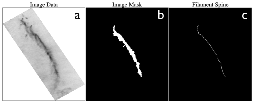
Figure 1: Step one in the typical RadFil workflow as summarized in §2.1. First, we input an image of the filament—in our example case, a map of the column density distribution of the Musca filament from the Herschel Gould Belt Survey (Cox et al., 2016), as shown in Figure (a). We additionally input a mask for the filament—see Figure (b)—calculated by applying a column density threshold $\approx 2\sigma$ above the mean background column density of the image. This is equivalent to $\rm 2.25\times 10^{21}\;cm^{-2}$. Finally, we create a filament spine—shown in (c)—by performing medial axis skeletonization on the filament mask, which produces a one-pixel one representation of the mask’s topology. This skeletonization is performed using functionality from the FilFinder package (Koch & Rosolowsky, 2015).

2.2 Profile Building

The second component of the RadFil workflow centers on building filament profiles using the $build\_profile()$ method. This is a multi-step process and the results of the profile building process for Musca (Cox et al., 2016) are summarized in Figure 2. First, we take the filament spine (a numpy mask of the same shape as the image array) which is either pre-computed or created as part of the data input process (§2.1). We then perform spline interpolation and fit a basis spline, “B-spline”, to the original spine points to determine a “smoothed” continuous version of the spine. The positions and the first derivatives of the B-spline knots are used to create the cuts from which the profiles are built. Users can control how frequently cuts are made using the “samp_int” argument—an integer which roughly specifies the sampling frequency in pixels. We emphasize this is an approximation. The knots which define the B-spline tend to be about one pixel length apart. This means that thinning the sampling points by the “samp_int” parameter will produce an average physical distance between cuts of the sampling interval times the image scale of each pixel.

At every sampling point (taken from the B-spline), RadFil parameterizes the line which is tangent to the curve at that point, using the first derivative. RadFil then finds the normal line—the line that is perpendicular to the tangent—and uses it to create the cut (Figure 3a). This process is repeated at every sampling point, creating an ensemble of cuts taken across the spine at approximately even intervals. Along each cut, RadFil calculates the radial distances from the spine and the intensities of the pixels that intersect it. Since the radial cut does not necessarily intersect neighboring pixels at their centers, we store the pixel positions corresponding to the midpoint of the cut’s path through each pixel. We then use these positions to compute the radial distances (see Figure 3a). To determine the intensity at each radial distance, we perform bilinear grid interpolation using the set of samples along each cut. For Musca, the choice of interpolation scheme has a minimal effect on our results. If one adopts a “nearest” interpolation scheme, as opposed to a bilinear one, it affects the best-fit values presented in §4 at $<1\%$ level.

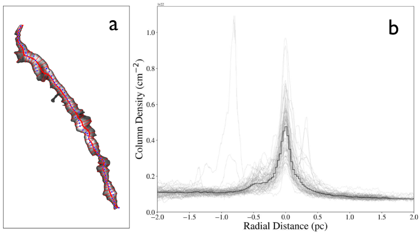
Figure 2: The profile building process for the Musca filament (Cox et al., 2016), as described §2.2. We take the filament spine shown in Figure 1c and smooth it via B-spline fitting. The smoothed spine is shown as the thick red line in Figure (a), which has been overlaid on the column density distribution inside the filament mask (background grayscale). Then we take perpendicular cuts across the spine, which are shown as thin red intersecting lines in Figure (a). Finally, we shift each cut to the pixel with the peak column density, considering only those pixels along each cut and confined inside the filament mask. We mark the peak intensity pixels via blue scatter points in Figure (a). The column density profiles resulting from the cuts are shown as thin gray lines in Figure (b). Users can also choose to bin the column density profiles of the individual cuts, and we show the binned average profile (with the “bins” argument set to 600) with the black step function in Figure (b).

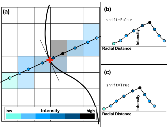
Figure 3: Schematic plots showing how the radial profile is calculated along a cut, and how profile shifting affects the profile. (a) The plot shows that the cut is derived based on the tangent at the sampling point (the red cross). RadFil calculates the radial distances from the spine and the intensities of the pixels that intersect it and stores the radial cut position that is closest to the middle of each pixel. (b) and (c) show the resulting profile along the cut shown in (a), when the shifting is set to False and True, respectively. When the “shift” argument is set to True, the radial profile is shifted such that the radial distance to the data point with the maximum intensity is 0.

2.2.1 Optional: Profile Shifting

While building the profiles, users also have the option to shift the radial profile along each cut so that it is centered on the pixel with the peak intensity. This is useful because the FilFinder skeletonization procedure often implemented to find the spine only takes into account the topology of the mask (and not the intensity distribution within it). Thus, the spine does not necessarily correspond to the peak intensity (e.g. in the case where there is an asymmetry in the radial profile with one side showing a substantial extended “wing” in its intensity distribution).

The option to shift the profile is controlled via the “shift” argument which accepts a boolean. If users choose to shift, RadFil will either search for the pixel with the peak intensity a) along each cut but inside the filament mask (if a mask is provided in §2.1) or b) along each cut but within a certain distance of the spine (if no mask is provided but a “cutdist” argument is given). Then it will recompute the radial distances and intensities assuming that pixel with the peak intensity (rather than the point of intersection with the spine) is situated at a radial distance of 0 pc (see Figures 3b and c). Because only points along the cut and confined inside the filament mask or within the “cutdist” distance are considered, this ensures that the peak of each individual profile is centered on 0 pc while also ensuring that only physically meaningfully points are considered when attempting to determine where to shift the profile.

2.2.2 Optional: Profile Binning

After the radial profiles along all the cuts are calculated, RadFil can optionally compute an averaged median profile for the filament by averaging the intensity values in radial distance bins whose number and width are controlled by the user. Users can specify a bin number via the “bins” argument which breaks up the profile into $n$ bins, spanning the minimum to maximum radial distances found in the ensemble of cuts. Alternatively, users can manually set the bin edges themselves, using, for example, the numpy linspace function, which creates an array of bin edges given some lower bound, upper bound, and number of bins. In more detail, RadFil sorts the ensemble of radial distance values into their appropriate radial distance bin, and then takes the median of their corresponding intensities to determine the average intensity at the center of the bin. If users choose to bin, fitting will be performed on the averaged binned profile in §2.3. If no binning is applied, fitting can be performed on the entire ensemble of cuts without averaging. In Figure 2b, we show the entire ensemble of cuts without averaging via the thin gray lines, and overlay the averaged bin profile (with the “bins” argument set to 600) as a black step function.

2.2.3 Optional: $pts\_mask$ and Profile Folding

Finally, a few other $build\_profile()$ optional arguments are worthy of note. First, if there are any sections of the filament one would like excluded from the building process (so no samples are taken, etc.), one can enter the optional “pts_mask” argument as a boolean mask of the same shape as the image array, which will discard any spine point that falls outside the region where “pts_mask=True.” This can be useful in cases where the filament is experiencing stellar feedback (thereby disrupting its morphology), or when the filament loops back on itself (causing the same region to be sampled twice). Second, when taking the “averaged” profile via radial distance binning, users have the option to input a boolean value for the “fold” argument—this controls whether the averaged profile should be folded around the central radial distance, producing a half profile with only positive radial distance values. This is equivalent to averaging the intensities values within the same absolute radial distance bin from the spine (e.g. -3 and 3 pc) and assigning it to a distance of 3 pc. This is useful in cases where there is an asymmetry in the profile, which would affect the evaluation of the residual and could introduce biases to the fitting.

2.3 Profile Fitting

The final step in the RadFil workflow involves fitting the filament’s “master” profile from the $profile\_building()$ step (see §2.2). The “master” profile is dependent on the decisions users make in the $profile\_building()$ step regarding, for example, shifting, binning, and folding the profiles (see §2.2). All the fitting is performed via the $fit\_profile()$ function, which utilizes the astropy.modeling subpackage.

2.3.1 Optional: Background Subtraction Prior to Profile Fitting

Prior to fitting the profile, RadFil supports background subtraction with a polynomial function of a non-negative degree. The degree of the polynomial is controlled via the “bgdegree” argument, and it accepts a non-negative integer including 0 (a zeroth order polynomial i.e. a constant) or 1 (a first order polynomial). The background fitting is done with the astropy implementation of a linear least-squares fitting routine. In cases where the user would like to fit a higher-degree polynomial to the background, the linear least-squares fitting can be inefficient at finding the global minimum of the objective function. Thus, users are expected to refrain from fitting a high-degree polynomial to the background, which could result in over-fitting and thus in loss of significant features after the fitted background is subtracted from the original radial profile.

Background subtraction is optional. However, if users choose to subtract a background, they can specify the range of radii over which to estimate the background. This is controlled via the “bgdist” argument, which accepts a tuple specifying the absolute lower and upper bounds of the background subtraction radii (e.g. bgdist=(1,2) indicates that the background will be estimated from -2 to -1 pc and from 1 to 2 pc). We perform basic outlier removal via sigma clipping, set to $3\sigma$. See Figure 4a for an example of typical background subtraction.

2.3.2 Profile Fitting

After choosing whether or not to background subtract, users have the option to fit two functions to the filament’s profile—a Plummer (see Figure 4a) or a Gaussian (see Figure 5a). The choice of function is specified via the “fitfunc” argument, which accepts a string (“Gaussian” or “Plummer”). Our Gaussian function is given by $H(r)=a\,\exp{(\frac{{-[r-\mu]}^{2}}{2\sigma^{2}})}$ where $r$ is the radial distance, $H$ is the profile height, and the free parameters are the amplitude ($a$), the standard deviation ($\sigma$) and optionally the mean ($\mu$). In the Gaussian case, users can decide whether to fit for the mean using the boolean argument “fix_mean,” which fixes the mean to zero when True and lets it float in the fit when False. The default behavior is to set “fix_mean=True” when “shift=True” and “fix_mean=False” otherwise. Our Plummer function is the same as that found in Cox et al. (2016) and is given by $H(r)=\frac{H_{0}}{[{1+({\frac{r}{R_{flat}})^{2}}]}^{\;\frac{p-1}{2}}}$, where $H_{0}$ is the peak profile height, $R_{flat}$ is the flattening radius, and $p$ is the index of the density profile. When fitting the Plummer, we assume that the inclination angle of the filament to the plane-of-the-sky is zero.

RadFil uses the astropy implementation of the Levenberg-Marquardt algorithm to fit the profile. The Levenberg-Marquardt algorithm can be seen as an interpolation between the Gauss-Newton algorithm and the gradient descent, and it is preferable in non-linear curve fitting, especially in cases where the initial guess cannot be determined without a large uncertainty. As in the background fitting, the objective function is the least-squares residual. RadFil currently only supports fitting to the “master” profile (e.g. the entire ensemble of cuts in the case of no binning, the binned median profile in the case of binning, or the “folded” version of either of these two cases). However, users can easily export the radial distances and intensities for each cut individually, to which users can apply their own fitting routines (see §3 for more information on how RadFil organizes its output).

Just like when subtracting the background, RadFil allows the user to specify the fitting radii over which to perform the fit. This is critical, as several studies have shown that the best-fit parameters for Gaussian and Plummer functions are extremely sensitive to choice of both fitting distance and background subtraction radii (Smith et al., 2014; Zucker et al., 2017; Panopoulou et al., 2017). The fitting distance is controlled via the “fitdist” argument, which accepts either a float or a tuple. If a float is entered, RadFil will fit to that radial distance symmetrically on either side of the spine. However, if users would like an asymmetric fitting range, they can enter a tuple with a lower and upper bound (e.g. -1 to 2 pc) and RadFil will only consider that range of radial distances when performing the fit.

Finally, RadFil is capable of computing the deconvolved widths if a beamwidth for the image is provided. If possible, RadFil will automatically read the beamwidth keyword from the FITS header. Otherwise, users can provide a value in arcseconds for the “beamwidth” argument manually in $fit\_profile()$. If no beamwidth is provided, RadFil will only compute the convolved FWHM value for the filament, using the formula $FWHM=2\sqrt{2\log(2)}\,\sigma$, where $\sigma$ is the standard deviation when a Gaussian function is chosen and the flattening radius when a Plummer function is chosen. If a beamwidth is provided, RadFil determines the deconvolved FWHM using the following formula $FWHM_{deconv}=\sqrt{FWHM^{2}-B^{2}}$ where B is the physical beamwidth and FWHM is the convolved FWHM computed above. This definition of the deconvolved FWHM is taken from Könyves et al. (2015). This deconvolution procedure is not robust. Convolving the data with a beam of known size and recalculating the deconvolved FWHM produces different values. To illustrate this, we have taken the original Musca column density map (see Figure 1a), with a beamwidth of $36.3\arcsec$ (0.035 pc), and degraded the resolution of the map by a factor of two and four, so the new maps have a beamwidth of $1.2\arcmin$ (0.070 pc) and $2.4\arcmin$ (0.14 pc), respectively. Adopting the same fitting parameters as before, we determine the deconvolved FWHM values in both cases, the results of which are reported in Table 1. For the Gaussian fits, the deconvolved FWHM for the $2.4\arcmin$ map is $1.6\times$ higher than for the $36\arcsec$ map. The Plummer fits appear slightly more robust, producing a deconvolved FWHM that is only $1.3\times$ higher. Users should be aware that the deconvolved FWHM can increase significantly as the resolution of the map decreases. Nevertheless, this is the deconvolution procedure adopted throughout the literature (see, for instance, Panopoulou et al., 2017; Koch & Rosolowsky, 2015).

2.3.3 Uncertainties in Best-Fit Parameter Values

There are two types of uncertainties inherent in RadFil’s fitting procedure. First, there is statistical uncertainty intrinsic to our least-squares fitting algorithm. Our choice of fitter, astropy’s LevMarLSQFitter, returns a covariance matrix, and the statistical uncertainties on the best-fit values can be calculated by taking the square-root of the diagonal elements of this matrix (Hogg et al., 2010). After running the fit_profile() method, users can access these uncertainties via RadFil’s “std_error” attribute, which returns an array whose length is equal to the number of fitted parameters. An alternative method is to calculate the statistical uncertainty empirically, using either bootstrap or jackknife resampling methods (see discussion in Section 4 of Hogg et al., 2010). We plan to add support for empirical error calculations in the future.

In additional to statistical uncertainty, there is also systematic uncertainty stemming from the user’s choice of fitting parameters. For reasonably built filament profiles (whose cuts are well-sampled but also statistically independent) the choice of background subtraction and fitting radii tend to dominate the systematic uncertainty. The “bgdegree” argument (controlling whether a zeroeth or first order polynomial is fit to the background) and the “fix_mean” argument (controlling whether the mean is fixed to zero in the Gaussian case) only become important if the data are highly skewed. To quantify the uncertainty based on background subtraction and fitting radii, RadFil has a built-in function called calculate_systematic_uncertainty() which accepts two lists, one containing various options for the background subtraction radii, and the other containing options for the fitting radius. RadFil will compute all possible combinations of background subtraction and fitting radii given these two lists, and then determine the best-fit values in each case for either a Gaussian or Plummer model. RadFil will then store a dictionary (“radfil_trials”), with each dictionary key corresponding to a different parameter in the model. Accessing these keys will return a pandas dataframe (where the columns are the fitting radii and the rows are the background subtraction radii), which users can easily print to screen to summarize the results.

Beamwidth	Gaussian		Plummer
	FWHM (pc)	$\rm FWHM_{deconv}$ (pc)	FWHM (pc)	$\rm FWHM_{deconv}$ (pc)
36.3″	0.159	0.155	0.221	0.218
1.2′	0.197	0.184	0.248	0.238
2.4′	0.282	0.244	0.321	0.289

Table 1: Dependence of deconvolved FWHM on the beamwidth of the image data. RadFil defines the $FWHM_{deconv}=\sqrt{FWHM^{2}-B^{2}}$ (Könyves et al., 2015) where B is the physical beamwidth of the image and $FWHM=2\sqrt{2\log(2)}\,\sigma$. The $\sigma$ parameter corresponds to the standard deviation when a Gaussian function is chosen and the flattening radius when a Plummer function is chosen. Adopting a distance to Musca of 200 pc (Cox et al., 2016), a beamwidth of $36\arcsec$, $1.2\arcmin$, and $2.4\arcmin$ corresponds to a physical size of 0.035 pc, 0.070 pc, and 0.14 pc, respectively. The deconvolution procedure RadFil adopts from Könyves et al. (2015) is not robust—the deconvolved FWHM increases as the resolution of the image decreases.

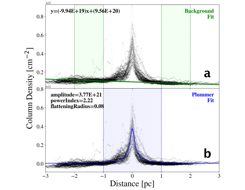
Figure 4: The results of applying our Plummer fitting procedure to the Musca filament from Cox et al. (2016), when adopting the same fitting radius (see also Figures 1 and 2). In Figure (a), we model the background as a first-order polynomial and estimate its contribution between 1 and 2 pc from the spine (green shaded regions, bounded by thin vertical green dashed lines). The best-fit background is shown as a green line in Figure (a) and the best-fit parameterization of that line is shown in the top left corner. This best-fit background is then subtracted off, producing the ensemble of radial profiles shown in Figure (b). We fit a Plummer function to the subtracted profiles within 1.0 pc from the spine (blue shaded region, bounded by thin vertical blue dashed lines). The best-fit Gaussian profile is shown in Figure (b) in blue and the best-fit values are summarized in the top left corner.

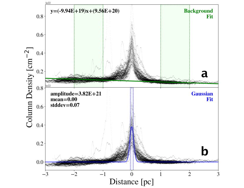
Figure 5: The results of applying our Gaussian fitting procedure to the Musca filament from Cox et al. (2016), when adopting the same fitting radius (see also Figures 1 and 2). In Figure (a), we model the background as a first-order polynomial and estimate its contribution between 1 and 2 pc from the spine (green shaded regions, bounded by thin vertical green dashed lines). The best-fit background is shown as a green line in Figure (a) and the best-fit parameterization of that line is shown in the top left corner. This best-fit background is then subtracted off, producing the ensemble of radial profiles shown in Figure (b). We fit a Plummer function to the subtracted profiles within 0.05 pc from the spine (blue shaded region, bounded by thin vertical blue dashed lines). The best-fit Gaussian profile is shown in Figure (b) in blue and the best-fit values are summarized in the top left corner.

3 The RadFil Architecture

When users input data (§2.1), build their filament profiles (§2.2), and fit their filament profiles (§2.3), RadFil stores all the relevant information computed at each step as attributes of the radfil class object, which users can access at any time or export for further processing.

For instance, once a radfil class object is instantiated, any data or properties that the user inputs into RadFil (e.g. the filament image, mask, spine, distance, etc.) are accessible by calling the name of the radfil class object (e.g. “radobj”) and then the name of the input argument. For instance, users can type radobj.image, radobj.distance, or radobj.filspine to return any of these arrays or quantities. If users choose to make their own filament spine using FilFinder and RadFil’s $make\_fil\_spine()$ function, users can also return the length of that spine by calling radobj.length.

Once users have built their profiles, a new set of attributes becomes available. For instance, users can access the ordered list of the x and y pixel coordinates defining the spine points (both before and after the smoothing via the B-spline fitting) by calling radobj.xbeforespline and radobj.ybeforespline, or radobj.xspline and radobj.yspline respectively. Most importantly, RadFil also stores all the radial distances and profile heights of individual cuts across the spine as a dictionary, which users can access by calling the “dictionary_cuts” attribute. The dictionary includes keys like “profile” and “distance”, both of which access a list containing a set of numpy arrays, where the number of arrays is equivalent to the number of cuts across the spine. Each individual array contains the radial distances or the profile heights corresponding to each cut. Another dictionary key of interest is the “mask_width” key which contains a list of floats, where each float indicates the width of the individual cut confined within the mask (i.e. the distance between where the cut intersects the edge of the mask on either side of the spine). The average of these values can then be used to estimate a “mask-based” width of the filament (e.g. in the case of Musca, the average width of some closed contour). This is equivalent to taking the average of all the lengths of the thin red cuts intersecting the filament spine in Figure 2a.

Finally, once users have performed background subtraction and/or fit their profile, they can access the resulting best-fit parameters via the radobj.bgfit and radobj.profilefit attributes, which will return the astropy.modeling objects. These modeling objects will then have their own attributes users can access to get information about the fit (i.e. the attributes “param_names” or “parameters” return the variable names and the best-fit parameter values, respectively). As one avenue to calculate the uncertainty on the best-fit parameters, users can access the covariance matrix for the fit using the command radobj.param_cov. This covariance matrix is used to calculate the standard errors on the best-fit parameters, which can be accessed via radobj.std_error. However, we strongly caution that using the covariance matrix will likely underestimate the errors, as simply tweaking knobs (like the fitting radius) will produce uncertainties in the best-fit parameters much larger than those derived from the covariance matrix. To quantify the systematic uncertainties, users can run calculate_systematic_uncertainty() (as discussed in §2.3.3), which will return a set of pandas dataframes summarizing the various best-fit values given different background subtraction and fitting radii. Finally, users can obtain the FWHM of the filament and (if a beamwidth is entered) the deconvolved FWHM using the radobj.FWHM and radobj.FWHM_deconv commands.

4 Proof-of-Concept

As a proof-of-concept, we have tested the results RadFil provides against the same results produced by a private and independent radial density profile fitting code. For a fair comparison, we apply our technique to an identical dataset and adopt the same fitting parameters. To reiterate, for this purpose we have chosen the Musca filament as presented in Cox et al. (2016), whose column density map is publicly available online as part of the Herschel Gould Belt Survey archive. This filament is also used as an example in the RadFil tutorial, which is likewise available online as a Jupyter notebook that users can download and run themselves. We adopt the same 200 pc distance to Musca as in Cox et al. (2016).

We first start by applying a column density threshold to the publicly available Musca column density map ($\approx 2\sigma$ above the background column density or $\rm 2.25\times 10^{21}\;cm^{-2}$), in order to produce a mask which delineates the morphology of the filament. The column density map is shown in Figure 1a while the resulting filament mask is shown in Figure 1b. We then run the $make\_fil\_spine()$ command to produce a filament spine via medial axis skeletonization, as discussed in Koch & Rosolowsky (2015). This spine is shown in Figure 1c. Using the FilFinder package we obtain a length of 8.1 pc, which is in excellent agreement with the length found in Cox et al. (2016) ($\approx 8$ pc, see their Figure 4a).

When building the profile, we adopt a pixel sampling interval (“samp_int”) of 25, equivalent to making a cut approximately every 0.10 pc given the image scale of the Musca map ($\rm\frac{0.00387\;pc}{pixel}$). In Figure 2a, these cuts are shown as thin red lines intersecting the smoothed filament spine (obtained via B-spline fitting), which is plotted in thick red. The column density distribution inside the filament mask is shown in grayscale in the background. After making the cuts, we choose to shift the filament profile to the peak intensity along each cut confined inside the filament mask. The point of peak intensity across each cut is marked via a blue scatter point in Figure 2a. Each individual cut is shifted so that this position is assigned a radial distance of zero, and the profile is now built out from this point. The individual shifted profiles corresponding to the cuts are shown in gray in Figure 2b.

As in Cox et al. (2016), we fit both a Gaussian and a Plummer function. We first subtract a first-order linear background, estimated between 1 and 2 pc on either side of the spine (Figures 4a and 5a). For their Plummer function Cox et al. (2016) choose a fitting distance of 1 pc (N. Cox; private communication), determining a best-fit flattening radius of 0.08 pc and power index of $2.2\pm 0.3$ (see Figure 4b in Cox et al., 2016). Fitting to the ensemble of cuts (Figure 2b) out to an identical fitting radius, we determine a best-fit flattening radius of 0.08 pc and best-fit power index of 2.22. Our best-fit Plummer function is shown in Figure 4b. The statistical uncertainty on these parameters, computed from the covariance matrix, is low, equivalent to 0.001 pc for the flattening radius and 0.01 for the power index. To calculate the systematic uncertainty, we use RadFil’s calculate_systematic_uncertainty() function. We test fitting radii of 0.5 pc, 1.0 pc, 1.5 pc, and 2.0 pc, and background subtraction radii of 1-2, 2-3 pc, 2-4 pc, and 3-4 pc. The results are summarized in Table 2. By taking the standard deviation of the set of best-fit values for each parameter (Table 2), we find that the systematic uncertainty is about an order of magnitude higher than the statistical uncertainty, or 0.01 pc for the flattening radius and 0.13 for the power index. Adding the uncertainties in quadrature, we determine $R_{flat}=0.08\pm 0.01$ pc and $p=2.22\pm 0.13$, in strong agreement with the Cox et al. (2016) results.

Next, for their Gaussian function Cox et al. (2016) choose a fitting distance of 0.05 pc (N. Cox; private communication) and obtain a deconvolved FWHM width of $0.14\pm 0.03$ pc. Again, adopting this same cutoff, we fit a Gaussian to our ensemble of cuts (Figure 2b) and obtain a best-fit deconvolved FWHM value of 0.16 pc, with a statistical uncertainty of 0.008 pc. Our best-fit Gaussian function is shown in Figure 5b. However, similar to the Plummer fits, the systematic uncertainties dominate. To calculate the systematic uncertainty, we again use RadFil’s calculate_systematic_uncertainty() function. We test fitting radii of 0.05 pc, 0.1 pc, 0.25 pc, 0.5 pc, and 1 pc, and background subtraction radii of 1-2 pc, 2-3 pc, 2-4 pc, and 3-4 pc. The results are summarized in Table 3. By taking the standard deviation of the set of best-fit values for the width, we calculate a systematic uncertainty on the FWHM value of 0.09 pc. Adding the uncertainties in quadrature, we calculate a deconvolved FWHM of $0.16\pm 0.09$ pc, which is again consistent with the published value from Cox et al. (2016). While the systematic uncertainties we calculate depend on our background subtraction radii and fitting radii input lists, it does highlight how a wide range of best-fit values are attainable simply by tweaking the fitting knobs. Thus, it is important to be explicit about which fitting parameters one adopts when reporting best-fit values obtained from radial profile fitting.

Amplitude ($\rm cm^{-2})$

Fitting Radius

Flattening Radius (pc)

Fitting Radius

Power Index

Fitting Radius

0.5 pc

1 pc

1.5 pc

2 pc

0.5 pc

1 pc

1.5 pc

2 pc

0.5 pc

1 pc

1.5 pc

2 pc

Background Subtraction Radii

1-2 pc

3.84E+21

3.77E+21

3.72E+21

3.70E+21

Background Subtraction Radii

1-2 pc

0.063

0.076

0.084

0.089

Background Subtraction Radii

1-2 pc

2.05

2.22

2.34

2.3

2-3 pc

3.86E+21

3.79E+21

3.75E+21

3.74E+21

2-3 pc

0.063

0.074

0.082

0.084

2-3 pc

2.03

2.19

2.28

2.31

2-4 pc

3.83E+21

3.76E+21

3.71E+21

3.70E+21

2-4 pc

0.064

0.077

0.085

0.087

2-4 pc

2.05

2.23

2.34

2.37

3-4 pc

3.82E+21

3.74E+21

3.69E+21

3.68E+21

3-4 pc

0.064

0.078

0.087

0.089

3-4 pc

2.07

2.26

2.39

2.41

Table 2: The effect of tweaking the background subtraction radii and fitting radius on our Plummer model parameters, with amplitude (left), flattening radius (middle), and index of the density profile (right). To estimate the background, we fit a first-order polynomial between radial distances of 1-2 pc, 2-3 pc, 2-4 pc, and 3-4 pc. We adopt fitting radii of 0.5 pc, 1 pc, 1.5 pc, and 2 pc. For each combination we compute the best-fit amplitude, flattening radius, and power index to quantify the systematic effect that tuning these parameters has on our results. This is performed via RadFil’s calculate_systematic_uncertainty() function.

Amplitude ($\rm cm^{-2})$

Fitting Radius

Standard Deviation (pc)

Fitting Radius

0.05 pc

0.1 pc

0.25 pc

0.5 pc

1 pc

0.05 pc

0.1 pc

0.25 pc

0.5 pc

1 pc

Background Subtraction Radii

1-2 pc

3.82E+21

3.70E+21

3.29E+21

2.96E+21

2.94E+21

Background Subtraction Radii

1-2 pc

0.068

0.083

0.12

0.16

0.16

2-3 pc

3.84E+21

3.72E+21

3.31E+21

2.96E+21

2.93E+21

2-3 pc

0.068

0.084

0.12

0.16

0.16

2-4 pc

3.82E+21

3.70E+21

3.29E+21

2.96E+21

2.94E+21

2-4 pc

0.068

0.083

0.12

0.16

0.16

3-4 pc

3.81E+21

3.68E+21

3.28E+21

2.96E+21

2.95E+21

3-4 pc

0.067

0.083

0.12

0.15

0.15

Table 3: The effect of tweaking the background subtraction radii and fitting radius on our Gaussian model parameters, with amplitude (left) and standard deviation (right). To estimate the background, we fit a first-order polynomial between radial distances of 1-2 pc, 2-3 pc, 2-4 pc, and 3-4 pc. We adopt fitting radii of 0.05 pc, 0.1 pc, 0.25 pc, 0.5 pc, and 1.0 pc. For each combination we compute the best-fit amplitude and standard deviation to quantify the systematic effect that tuning these parameters has on our results. This is performed via RadFil’s calculate_systematic_uncertainty() function.

5 A Roadmap for Future Development

RadFil is undergoing continuous development and all the code is currently publicly available at this GitHub repository. The code used to produce the results in this paper has also been archived on Zenodo with a unique DOI (https://doi.org/10.5281/zenodo.1287318). The package is also available on PyPi and can be installed with pip. Since RadFil is open-source, users are welcome to clone the repository on GitHub and make any changes to the code that they desire. Likewise they are encouraged to report any issues or feature requests via the issue tracker on GitHub. The code itself can be run in Python 2.7, 3.4, 3.5, or 3.6.

At the moment RadFil is only designed to work with 2D images. Current datasets ripe for analysis include maps of dust emission (using e.g. the Hi-GAL survey; Molinari et al., 2016) and dust extinction (using e.g. the GLIMPSE survey; Churchwell et al., 2009), or else integrated intensity maps from a wide-variety of spectral-lines (for example $\rm{}^{13}CO,C^{18}O$ from surveys like GRS, SEDIGISM, or COHRS; Jackson et al., 2006; Schuller et al., 2017; Dempsey et al., 2013). Nor is RadFil limited to observational data. As long as the data are on a regular grid, one could apply RadFil to 2D slices obtained from 3D numerical simulations, or integrated intensity maps from synthetic spectral cubes.

In the coming years we hope to expand RadFil’s functionality so that it can be applied to 3D datasets, most notably position-position-velocity (p-p-v) spectral cubes from both low and high density gas tracers, or else 3D density cubes obtained from hydrodynamical simulations. Existing structure identification packages like $DisPerSE$ (Sousbie, 2013) already have the capability to extract filaments in 3D and have been applied to cosmic web filaments in dark matter simulations (Sousbie et al., 2011) as well as star-forming filaments in gravoturbulent molecular cloud simulations (Klassen et al., 2017). While still under development, the FilFinder algorithm (Koch & Rosolowsky, 2015) also has the ability to extend its filament identification procedure to three dimensions, and Koch & Rosolowsky (2015) cite the future application of their algorithm to 3D p-p-v spectral cubes as a primary motivation. We envision that RadFil would be a natural extension of these filament identification packages, by providing additional functionality and flexibility for users interested in more robust width determination. In this vein, we hope to continue to improve the ease by which RadFil can be integrated into existing filamentary analysis pipelines, and we welcome community investment in its development both now and in the future.

References

- André et al. (2010) André, P., Men’shchikov, A., Bontemps, S., et al. 2010, Astronomy and Astrophysics, 518, L102
- Arzoumanian et al. (2011) Arzoumanian, D., André, P., Didelon, P., et al. 2011, A&A, 529, L6
- Battersby et al. (2014) Battersby, C., Ginsburg, A., Bally, J., et al. 2014, ApJ, 787, 113
- Churchwell et al. (2009) Churchwell, E., Babler, B. L., Meade, M. R., et al. 2009, PASP, 121, 213
- Cox et al. (2016) Cox, N. L. J., Arzoumanian, D., André, P., et al. 2016, A&A, 590, A110
- Dempsey et al. (2013) Dempsey, J. T., Thomas, H. S., & Currie, M. J. 2013, ApJS, 209, 8
- Goodman et al. (2014) Goodman, A. A., Alves, J., Beaumont, C. N., et al. 2014, ApJ, 797, 53
- Hagberg et al. (2008) Hagberg, A. A., Schult, D. A., & Swart, P. J. 2008, in Proceedings of the 7th Python in Science Conference (SciPy2008), Pasadena, CA USA, 11–15
- Hogg et al. (2010) Hogg, D. W., Bovy, J., & Lang, D. 2010, ArXiv e-prints, arXiv:1008.4686
- Hunter (2007) Hunter, J. D. 2007, Computing in Science and Engineering, 9, 90
- Jackson et al. (2006) Jackson, J. M., Rathborne, J. M., Shah, R. Y., et al. 2006, ApJS, 163, 145
- Klassen et al. (2017) Klassen, M., Pudritz, R. E., & Kirk, H. 2017, MNRAS, 465, 2254
- Koch & Rosolowsky (2015) Koch, E. W., & Rosolowsky, E. W. 2015, MNRAS, 452, 3435
- Koch & Rosolowsky (2016) —. 2016, FilFinder: Filamentary structure in molecular clouds, Astrophysics Source Code Library, , , ascl:1608.009
- Könyves et al. (2015) Könyves, V., André, P., Men’shchikov, A., et al. 2015, A&A, 584, A91
- McKinney (2010) McKinney, W. 2010, in Proceedings of the 9th Python in Science Conference, ed. S. van der Walt & J. Millman, 51 – 56
- Men’shchikov (2013) Men’shchikov, A. 2013, A&A, 560, A63
- Molinari et al. (2016) Molinari, S., Schisano, E., Elia, D., et al. 2016, A&A, 591, A149
- Panopoulou et al. (2017) Panopoulou, G. V., Psaradaki, I., Skalidis, R., Tassis, K., & Andrews, J. J. 2017, MNRAS, 466, 2529
- Pedregosa et al. (2011) Pedregosa, F., Varoquaux, G., Gramfort, A., et al. 2011, Journal of Machine Learning Research, 12, 2825
- Schisano et al. (2014) Schisano, E., Rygl, K. L. J., Molinari, S., et al. 2014, ApJ, 791, 27
- Schuller et al. (2017) Schuller, F., Csengeri, T., Urquhart, J. S., et al. 2017, A&A, 601, A124
- Seifried & Walch (2015) Seifried, D., & Walch, S. 2015, MNRAS, 452, 2410
- Smith et al. (2014) Smith, R. J., Glover, S. C. O., & Klessen, R. S. 2014, MNRAS, 445, 2900
- Sousbie (2013) Sousbie, T. 2013, ArXiv e-prints, arXiv:1302.6221
- Sousbie et al. (2011) Sousbie, T., Pichon, C., & Kawahara, H. 2011, MNRAS, 414, 384
- The Astropy Collaboration et al. (2018) The Astropy Collaboration, Price-Whelan, A. M., Sipőcz, B. M., et al. 2018, ArXiv e-prints, arXiv:1801.02634
- van der Walt et al. (2014) van der Walt, S., Schönberger, J. L., Nunez-Iglesias, J., et al. 2014, CoRR, abs/1407.6245, arXiv:1407.6245. http://arxiv.org/abs/1407.6245
- Wang et al. (2015) Wang, K., Testi, L., Ginsburg, A., et al. 2015, MNRAS, 450, 4043
- Zucker et al. (2015) Zucker, C., Battersby, C., & Goodman, A. 2015, ApJ, 815, 23
- Zucker et al. (2017) —. 2017, ArXiv e-prints, arXiv:1712.09655