Counting of States in Higgs Theories

Abstract

We enumerate the micro-states in Higgs theories, addressing (i) the number of vacuum states and (ii) the appropriate measure in the quantum path integral. To address (i) we explicitly construct the set of ground state wave-functionals in the field basis focussing on scalar modes $\theta(x)$. Firstly, we show that in the limit in which the gauge coupling is zero, we obtain an infinite set of degenerate ground states at large volume distinguished by $\theta(x)\to\theta(x)+\theta_{0}$, spontaneously breaking the global symmetry, as is well known. We then show that at finite gauge coupling there is a unique ground state at large volume since the wave-functional only depends on $\nabla\theta$ in the IR, and we explain this at the level of the Lagrangian. Since gauge fields fall off exponentially from sources there are no conserved charges or symmetries in the Higgs phase; so the Higgs mechanism is the removal of symmetry from the theory. We show how physical features of defects, such as cosmic strings in the abelian Higgs model, are best understood in this context. Since there is a unique ground state, we address (ii) whether the path integral is a volume measure for the radial Higgs field $\mathcal{D}\rho\,\rho^{N-1}$ from the $N$ components of the Higgs multiplet, or a line measure $\mathcal{D}\rho$ as the $N-1$ would-be Goldstones can be removed in unitary gauge. We prove that the need to avoid quartic divergences demands a tower of counter terms that resum to exactly give the volume measure. So the size of the Hilbert space in the zero gauge coupling case and finite gauge coupling case are in one-to-one correspondence, despite the degeneracy of the ground state being lifted in the latter. As a cosmological application, we point out that the volume measure can make it exponentially more unlikely in $N(=4)$ for the Standard Model Higgs to relax to the electroweak vacuum in the early universe.

I Introduction

An important discovery in fundamental physics was that of the Higgs particle ATLAS; CMS, which completes the Standard Model. Without the Higgs particle, the Standard Model would violate unitarity at energies well above the electroweak scale. The presence of the Higgs provides better UV behavior, allowing the Standard Model to make sense up to much higher energies. Interestingly, at temperatures well above the electroweak scale $\mathcal{O}(100)$ GeV the particles of the Standard Model are massless. Furthermore, there is an associated set of symmetries which become manifest. In particular, we know that interacting massless spin 1 particles, must be coupled to exactly conserved charges, which by the Noether theorem are associated with symmetries. At lower temperatures, these particles become massive due to interesting dynamics of the Higgs. This affects the symmetry structure in dramatic ways and will be examined rigorously in this paper.

Our primary interest is the Higgs mechanism in the Standard Model of particle physics. Here the full gauge group $SU(3)_{c}\times SU(2)_{L}\times U(1)_{Y}$ is linearly realized at high temperatures. Then, due to the Higgs acquiring a non-zero vacuum expectation value (VEV), only the reduced gauge group $SU(3)_{c}\times U(1)_{em}$ is linearly realized at low temperatures. The physical consequences can be stated more directly as follows: the 3 massless spin 1 particles $W_{1,2,3}$ associated with the group $SU(2)_{L}$ at high temperatures become 3 massive spin 1 particles $W^{\pm},Z$ at low temperatures, while fermions acquire a mass too. Beyond the Standard Model, there can be Higgs mechanisms associated with other gauge groups. One interesting possibility is associated with grand unification, such as $SU(5)$ Georgi:1974sy or $SO(10)$ Fritzsch:1974nn, etc, whose larger set of massless spin 1 particles become massive at temperatures well below the grand unification scale. Another possibility is associated with various hidden sector gauge groups, which are suggested by ideas in fundamental physics, including string theory and models of dark matter, etc, which may be associated with other Higgs sectors. Furthermore, within condensed matter physics, the phenomenon of superconductivity is associated with the photon of $U(1)_{em}$ acquiring a mass at very low temperatures. This superconductivity example carries some of the physics relevant to elementary particle physics, despite the latter being expanded around the Lorentz invariant vacuum. In fact we will study the (Lorentz invariant) abelian $U(1)$ example often in this paper to illustrate the underlying physics in the simplest possible setting.

Now it is usually stated that the Higgs mechanism is responsible for the “spontaneous breaking” of symmetries at low temperatures. The definition of spontaneous symmetry breaking (SSB) is that the theory is invariant under some symmetry $\hat{S}$, but the ground state (or the low temperature phase) of the theory is not, i.e., $\hat{S}|vac\rangle=|vac^{\prime}\rangle$, where $|vac^{\prime}\rangle\neq|vac\rangle$. While this is certainly true for some systems, such as ferromagnets, which spontaneously break rotational symmetry, it is rather unclear that this is correct for the Higgs mechanism where we need to deal with “gauge symmetries”. For one thing, consider the so-called “small-gauge” transformations associated with functions $\alpha(x)$ that vanish at spatial infinity. These are not in fact actual symmetries but are merely redundancies in the mathematical description and can be entirely removed by gauge fixing. Hence they can never be spontaneously broken since all states in a theory are trivially invariant under a small-gauge transformation $|\psi^{\prime}\rangle=|\psi\rangle$ (modulo an unimportant phase), including the vacuum. This is summarized by the so-called Elitzur’s theorem Elitzur:1975im. We will see this again later in this paper.

So the interesting and non-trivial issue to focus on is the fate of actual symmetries in a gauge theory. These are always associated with functions $\alpha(x)$ that are non-vanishing at infinity. The central example is when $\alpha(x)$ is a constant. This is a “global” transformation, and is a sub-group of the full gauge group. These are sometimes referred to as “global-gauge” transformations. (In the limit in which we send the gauge coupling to zero, these are ordinary global transformations.) If the Higgs has not acquired a VEV and so there are only massless spin 1 particles, these global transformations do in fact take generic states to different states $|\psi^{\prime}\rangle\neq|\psi\rangle$ (at least for weakly coupled theories). However the vacuum itself is invariant under this symmetry transformation. (The vacuum may not be invariant under other symmetry transformations, such as the so-called “large-gauge” transformations, in which $\alpha(x)$ is non-vanishing at infinity but also non-constant; we will return to these later in the paper.)

The important question then is: are the global symmetries spontaneously broken in the Higgs phase? The answer does not seem obvious (and is not addressed by Elitzur’s theorem Elitzur:1975im). These are real symmetries at high temperatures in the regular phase (associated with conserved charges), but appear to be hidden at low temperatures. But does it mean these symmetries were spontaneously broken and there are many distinct vacua, or could it be that these symmetries were removed altogether from the theory and there is a unique vacuum? The answer to this question does not arise trivially from claiming that gauge symmetry is only a redundancy, as this is ordinarily only true of the small-gauge transformations. For the fate of global symmetries, it requires a clear computation of the set of micro-states of the theory; we shall do this systematically in this paper. In particular, we will (i) explicitly count the vacuum states of the theory by finding the set of states $|vac\rangle$ that are orthogonal to one another. We will also (ii) count all the states in the Hilbert space by identifying the correct measure on the quantum path integral.

There has been a long discussion in the literature on the topic of SSB in the context of gauge theories. This includes Refs. Englert:1964et; Higgs:1964pj; Guralnik:1964eu; Bernstein:1974rd; Strocchi:1977za; Stoll:1995yg; Maas:2012ct; Kibble:2014gug; Strocchi:2015uaa; Maas:2017wzi and references therein. While there is broad agreement on the physical character of the Higgs mechanism and the resulting predictions for experiment, there does remain some confusion on the important issue of whether SSB in gauge theories is physical or just nomenclature. In particular, there does not appear to be a direct computation of the overlap wave-function between ground states, and the associated complete characterization of the interpolation between the global and gauge cases. This overlap is the precise quantity required to sharply address the question of SSB, and will be performed explicitly in this paper (among other items).

To calculate this (i) we will construct the ground state wave-functionals in the theory in the field basis. To work with a solvable system; we take the Higgs to be heavy, and so it can be taken to be frozen at its VEV $v$, as it has suppressed fluctuations. For the abelian $U(1)$ Higgs model, this leaves a truncated theory with only a quadratic Lagrangian in the transverse and longitudinal modes of a single spin 1 particle (for simplicity we ignore fermions, though their inclusion is straightforward). The longitudinal mode can be examined in various gauges, such as in Coulomb gauge $\nabla\cdot{\bf A}=0$ in which we must track a would-be Goldstone boson $\theta(x)$, or in unitary gauge $\theta(x)=0$ in which we must track the longitudinal part of the vector potential $A_{L}(x)$ directly. We show explicitly that in any gauge the ground state wave-functional is trivially invariant under small-gauge transformations, in accord with Elitzur’s theorem. More interestingly, we then consider global transformations. We show that if the gauge coupling $g$ is set to zero, we obtain a family of orthogonal ground state wave-functionals in the large volume limit and so there is SSB. Conversely, for finite gauge coupling, we obtain a unique ground state wave-functional in the large volume limit and so there is no SSB. We also show that for finite volume, there is a smooth transition between these limiting cases as we change the gauge coupling away from zero. In particular, so long as the spin 1 particle’s Compton wavelength $\lambda_{C}=2\pi/m=2\pi/(g\,v)$ is much bigger than the size of the system, we have SSB, but when it is much smaller than the size of the system, we have no SSB, and when it is comparable to the size of the system, we have partial SSB.

In order to explain these results, we consider the structure of the global symmetry operator $\hat{S}$. In the quantum theory it is associated with a conserved charge operator $\hat{Q}$ as $\hat{S}=\exp(i\,\hat{Q}\,\theta_{0})$. If the gauge coupling is taken to zero, we note there is a good conserved charge. However, for finite gauge-coupling the situation is more complicated. Recall that in a gauge theory, the charge $Q$ is given by a closed surface integral of the electric field $Q=\oint d{\bf S}\cdot{\bf E}$. For massless spin 1 particles, the electric field falls off as $1/r^{2}$ from point sources, leading to a conserved charge and a global symmetry. In fact there is a family of other charges defined at spatial infinity associated with large-gauge symmetries. However, when the spin 1 particle acquires a mass by the Higgs mechanism, the electric field falls off exponentially from point sources and so these charges are zero when the surface is taken to infinity and we show they are time dependent for finite surfaces. So there are no good conserved charges and no global (or large-gauge) symmetries. Hence the Higgs mechanism is in fact the removal of conserved charges and symmetries from the theory, rather than the spontaneous breakdown. By identifying canonically normalized fields, we also show this clearly at the level of the Lagrangian.

An interesting issue then is how to understand the existence and structure of defects, which are often thought to arise from SSB. For example, in the abelian $U(1)$ Higgs model, it is known that cosmic string solutions exist, and are usually ascribed to a phase-field that winds around the central axis of the string continuously varying from one vacuum to another. While this is the correct picture in the limit in which the gauge coupling is taken to zero, we explain that the basic properties of these cosmic strings at finite gauge coupling are best understood in terms of fields relaxing to a unique vacuum.

Another interesting issue is (ii) to count the full set of states in the theory beyond the vacuum states. In particular, since there is a unique vacuum and since in unitary gauge the would-be Goldstone modes $\theta(x)$ are removed from the theory, one might wonder what should be the measure on the quantum path integral. Should it be a volume measure $\mathcal{D}\rho\,\rho^{N-1}$, for the $N$ components of the Higgs multiplet, as it is in the global case, or should it be a line measure $\mathcal{D}\rho$ since the angular modes can be removed? By demanding that the theory is renormalizable, we prove that it is in fact the volume measure. This shows that in a definite sense the size of the Hilbert space in the global and gauge cases is in fact the same; it is simply that a symmetry gets removed in the gauge case.

An important application is to cosmology. We review the well known idea that the Higgs potential of the Standard Model turns over and becomes negative at very high energies, perhaps around $E\sim 10^{11}$ GeV, or so, depending on parameters. We then utilize the volume measure to estimate the probability that the Higgs began on the favorable side of the potential in the early universe in order to roll down to our electroweak vacuum. We find that it is exponentially unlikely. However, this should be understood more carefully in the context of inflation, reheating, etc, which we comment on briefly.

Our paper is organized as follows: In Section II we construct the Lagrangian for the vector and scalar modes in a simple Higgs model. In Section III we explicitly compute the ground state wave-functional(s). In Section IV we determine the number of vacua, comparing global to gauge cases. In Section V we examine whether the global transformations are real or redundant. In Section VI we discuss the spectrum of the theory. In Section LABEL:Charges we discuss the behavior of charges in the two phases. In Section LABEL:NonAbelian we extend our results to non-abelian theories. In Section LABEL:LargeGauge we discuss large-gauge transformations. In Section LABEL:TopologocalDefects we discuss properties of defects. In Section LABEL:PathIntegralMeasure we derive the measure on the quantum path integral. In Section LABEL:ApplicationtoCosmology we apply this to the Standard Model Higgs in the very early universe. Finally, in Section LABEL:Discussion we present an outlook.

II Simple Higgs Theory

Our interest is in general Higgs theories, which may involve some non-abelian gauge groups. In the Standard Model this involves the non-abelian gauge group $SU(2)_{L}\times U(1)_{Y}$ at high temperatures (with the residual gauge group $U(1)_{em}$ at low temperatures). A complete analysis of this would involve the full treatment of the 3 massless bosons associated with $SU(2)_{L}$, which include self-interactions. However, this involves additional complications that are not essential for the main issues of state counting that we wish to analyze in this paper. Instead we will focus on a simple version of the Higgs mechanism, which involves the abelian gauge group $U(1)$ at high temperatures (with no residual group at low temperatures); see Section LABEL:NonAbelian for the non-abelian case. This in fact is an accurate description of superconductivity, and will highlight the important features of the Higgs in general settings.

Consider then a collection of identical spin 1 particles, “photons”, that are massless at high temperatures. To describe their features in a local way, we organize them into a vector field $A_{\mu}$, with associated field strength $F_{\mu\nu}=\partial_{\mu}A_{\nu}-\partial_{\nu}A_{\mu}$. Since massless spin 1 particles have only 2 (transverse) polarizations, we must ensure that 2 of the 4 components of $A_{\mu}$ are unphysical. This is readily achieved by making $A_{0}$ non-dynamical and by making another component redundant, i.e., by introducing a “gauge symmetry”. We minimally couple this field to a complex scalar $\phi$ in the standard way with the following Lagrangian density (units $\hbar=c=1$, signature + - - -)

$$\mathcal{L}=-\dfrac{1}{4}F_{\mu\,\nu}F^{\mu\,\nu}+|D_{\mu}\phi|^{2}-V(\absolutevalue{\phi}),$$ (1)

where the covariant derivative is

$$D_{\mu}=\partial_{\mu}-i\,g\,A_{\mu},$$ (2)

and $g$ is the gauge coupling. The complex scalar $\phi$ implements the Higgs mechanism. It is assumed to have a potential of the form

$$V(|\phi|)=-\mu^{2}|\phi|^{2}+\lambda|\phi|^{4},$$ (3)

where we have truncated all operators at the dimension 4 level (we will return to this issue in Section LABEL:ApplicationtoCosmology when we examine the potential more carefully). Note that the form of the Lagrangian density is unchanged under the familiar abelian gauge transformations with parameter $\alpha$

$$A_{\mu} \to A_{\mu}+\partial_{\mu}\alpha,$$ (4)

$$\phi \to \phi\,e^{i\,g\,\alpha}.$$ (5)

If $\alpha$ is a constant, this is a global transformation and will be studied very carefully in this paper; if $\alpha$ is non-constant and has support at infinity, this is a large-gauge transformation and will be studied briefly in this paper; if $\alpha$ is non-constant and vanishes at infinity, this is a small-gauge transformation and is merely a redundancy.

In the regular phase $\mu^{2}<0$ leading to a minimum at $\phi=0$. In the Higgs phase $\mu^{2}>0$ leading to a minimum at $\phi\neq 0$. To expand around the non-zero minimum in the Higgs phase, it is useful to decompose the field in terms of polar variables, with radial field $\rho$ and phase $\theta$ as

$$\phi({\bf x})={1\over\sqrt{2}}\,\rho({\bf x})\,e^{i\,\theta({\bf x})}.$$ (6)

Re-writing the Lagrangian density in terms of these polar variables gives

$$\mathcal{L}=-\dfrac{1}{4}F_{\mu\,\nu}F^{\mu\,\nu}+{1\over 2}(\partial_{\mu}\rho)^{2}+{1\over 2}\rho^{2}(g\,A_{\mu}-\partial_{\mu}\theta)^{2}-V(\rho),$$ (7)

and the corresponding potential for the radial field $\rho$ is

$$V(\rho)=-\dfrac{1}{2}\mu^{2}\rho^{2}+\dfrac{1}{4}\lambda\,\rho^{4}.$$ (8)

Focussing on the Higgs phase with $\mu^{2}>0$, the minimum energy configuration occurs at the VEV $\rho_{0}=v=\mu/\sqrt{\lambda}$. We expand the radial Higgs field around this as

$$\rho(x)=v+h(x),$$ (9)

and we refer to $h$ as the Higgs field, with associated quanta “Higgs particles”. This expansion leads to a Lagrangian density that decomposes into several pieces as follows

$$\mathcal{L}=\mathcal{L}_{A_{\mu},\theta}+\mathcal{L}_{h}+\mathcal{L}_{\text{int}},$$ (10)

where

$$\mathcal{L}_{A_{\mu},\theta} = -\dfrac{1}{4}F_{\mu\,\nu}F^{\mu\,\nu}+\dfrac{v^{2}}{2}(g\,A_{\mu}-\partial_{\mu}\theta)^{2},$$ (11)

$$\mathcal{L}_{h} = {1\over 2}(\partial_{\mu}h)^{2}-\dfrac{1}{2}\,\lambda\,v^{2}\,h^{2},$$ (12)

$$\mathcal{L}_{\text{int}} = \dfrac{1}{2}(2\,v\,h+h^{2})(g\,A_{\mu}-\partial_{\mu}\theta)^{2}-\lambda\,v\,h^{3}-{1\over 4}\lambda\,h^{4}.\,\,\,\,$$ (13)

Here $\mathcal{L}_{A_{\mu},\theta}$ is the quadratic kinetic term for the photon and the would-be Goldstone $\theta$, $\mathcal{L}_{h}$ is the quadratic kinetic term for the Higgs, and $\mathcal{L}_{\text{int}}$ is the cubic and quartic interaction terms.

Note that the spin 1 mass and the Higgs mass are

$$m_{A} = g\,v,$$ (14)

$$m_{h} = \sqrt{2\,\lambda}\,v.$$ (15)

On the one hand, these are both set by the VEV $v$. On the other hand, they are parametrically different from one another, since the former is proportional to the gauge coupling $g$ and the latter is proportional to the (square-root of) self-coupling $\lambda$. Hence we can consider a situation in which the Higgs is somewhat heavier than the spin 1 particle (in the Standard Model the measured mass of the Higgs $m_{h}\approx 125$ GeV Aad:2015zhl is only a little heavier than the $W$ boson $m_{W}\approx 80$ GeV Beringer:1900zz). In this situation it suffices to consider the Higgs effectively frozen at its VEV, ignoring the back-reaction from its fluctuations. This means that the interaction terms can be ignored, and we can focus on the quadratic kinetic term $\mathcal{L}_{A_{\mu},\theta}$ for the purpose of understanding the symmetry structure of the theory. This is precisely what makes the abelian $U(1)$ Higgs model so simple. In non-abelian cases, we would further need to consider interactions among the spin 1 particles. However we believe all our qualitative conclusions carry over to these more complicated situations.

Now an important feature of any unitary theory is that the time component of the vector potential $A_{0}$ is non-dynamical. By varying the above action with respect to $A_{0}$ we obtain the local version of Gauss’ law

$$\nabla\cdot{\bf E}=-\nabla^{2}A^{0}-\nabla\cdot\dot{\bf A}=-g\,v^{2}(g\,A^{0}-\dot{\theta}).$$ (16)

We can use this to solve for $A^{0}$. Since the reduced theory $\mathcal{L}_{A_{\mu},\theta}$ is quadratic, we can diagonalize the theory in $k$-space. We define the spatial Fourier transform of a function $f$ as

$$f_{\bf k}(t)\equiv\int\!d^{3}x\,e^{i\,{\bf k}\cdot{\bf x}}f({\bf x},t).$$ (17)

Then the solution for $A^{0}_{\bf k}$ is

$$A^{0}_{\bf k}=\dfrac{i\,{\bf k}\cdot\dot{\bf A}_{\bf k}+g\,v^{2}\,\dot{\theta}_{\bf k}}{\omega_{k}^{2}},$$ (18)

where the dispersion relation is

$$\omega_{k}=\sqrt{k^{2}+g^{2}\,v^{2}},$$ (19)

with $k\equiv|{\bf k}|$.

Having eliminated $A^{0}$, there are 4 dynamical fields remaining in $\mathcal{L}_{A_{\mu},\theta}$, namely $A_{1},A_{2},A_{3},\theta$. However there are only 3 physical degrees of freedom as there is a gauge redundancy between them. For these 3 physical degrees of freedom, it is useful to isolate the 2 transverse vector modes, and the 1 longitudinal scalar mode. To do so we define a transverse vector ${\bf A}^{T}_{\bf k}$ and a longitudinal scalar $A^{L}_{\bf k}$ as

$${\bf A}^{T}_{\bf k} = {\bf A}_{\bf k}-\hat{\bf k}\,(\hat{\bf k}\cdot{\bf A}_{\bf k}),$$ (20)

$$A^{L}_{\bf k} = i\,\hat{\bf k}\cdot{\bf A}_{\bf k},$$ (21)

where $\hat{\bf k}\equiv{\bf k}/k$ is a unit vector in the ${\bf k}$-direction.

By using the solution for $A^{0}$ in $k$-space, we find that the Lagrangian for the transverse (T) and longitudinal (L) modes decouples and can be written as

$$L_{A_{\mu},\theta}=\int\!\dfrac{d^{3}k}{(2\pi)^{3}}\left(\mathcal{L}_{T,\bf k}+\mathcal{L}_{L,\bf k}\right),$$ (22)

where

$$\mathcal{L}_{T,\bf k} = {1\over 2}|\dot{\bf A}^{T}_{\bf k}|^{2}-{1\over 2}\omega_{k}^{2}|{\bf A}^{T}_{\bf k}|^{2},$$ (23)

$$\mathcal{L}_{L,\bf k} = \dfrac{v^{2}}{2\,\omega^{2}_{k}}|g\,\dot{A}^{L}_{\bf k}+k\,\dot{\theta}_{\bf k}|^{2}-\dfrac{v^{2}}{2}|g\,A^{L}_{\bf k}+k\,\theta_{\bf k}|^{2}.$$ (24)

Note that this Lagrangian is invariant under the (local) gauge transformations Eqs. (4, 5), since the fields transform as

$${\bf A}^{T}_{\bf k} \to {\bf A}^{T}_{\bf k},$$ (25)

$$A^{L}_{\bf k} \to A^{L}_{\bf k}-k\,\alpha_{\bf k},$$ (26)

$$\theta_{\bf k} \to \theta_{\bf k}+g\,\alpha_{\bf k},$$ (27)

which trivially leaves $\mathcal{L}_{T}$ unchanged and also leaves $\mathcal{L}_{L}$ unchanged as $g\,A^{L}_{\bf k}+k\,\theta_{\bf k}\to g\,A^{L}_{\bf k}+k\,\theta_{\bf k}$. It will be useful to analyze this theory in various gauges, especially unitary gauge $\theta_{\bf k}=0$ and Coulomb gauge $A^{L}_{\bf k}=0$ in which the form of Eq. (24) appears quite different.

III Ground State Wave-functional(s)

Among other things, we will be interested in the ground state of the theory. Since the above theory is quadratic, it is really a set of harmonic oscillators, whose ground state wave-function are Gaussians. To make the structure even clearer, let us pass to the Hamiltonian. It again decouples into a transverse (T) and longitudinal (L) piece as

$$H_{A_{\mu},\theta}=H_{T}+H_{L},$$ (28)

where

$$H_{T} = \int\!\dfrac{d^{3}k}{(2\pi)^{3}}\left[\dfrac{1}{2}|{\vec{\Pi}}^{T}_{\bf k}|^{2}+\dfrac{1}{2}\omega^{2}_{k}|{\bf A}^{T}_{\bf k}|^{2}\right],$$ (29)

$$H_{L} = \int\!\dfrac{d^{3}k}{(2\pi)^{3}}\left[\dfrac{\omega^{2}_{k}}{2\,v^{2}}|{\Pi}^{L}_{\bf k}|^{2}+\dfrac{v^{2}}{2}|g\,A^{L}_{\bf k}+k\,\theta_{\bf k}|^{2}\right],$$ (30)

with momentum conjugates

$${\vec{\Pi}}^{T}_{\bf k} = \dot{\bf A}^{T*}_{\bf k},$$ (31)

$${\Pi}^{L}_{\bf k} = {v^{2}\over\omega^{2}_{k}}(g\,\dot{A}^{L}_{\bf k}+k\,\dot{\theta}_{\bf k})^{*}.$$ (32)

Since the Hamiltonian is additive in the transverse and longitudinal modes, the ground state wave-functional $\Psi$ factorizes as

$$\Psi(A_{\mu},\theta)=\Psi_{T}({\bf A}^{T}_{\bf k})\,\Psi_{L}(A^{L}_{\bf k},\theta_{\bf k}).$$ (33)

Now recall that for a single harmonic oscillator with standard Hamiltonian $H=p^{2}/(2m)+m\,\omega^{2}\,x^{2}/2$, the ground state wave-function in the $x$-basis is $\psi(x)\propto\exp(-m\,\omega\,x^{2})$. Similarly we can determine the ground state wave-functionals for the above Hamiltonians in the field basis to be

$$\Psi_{T}({\bf A}^{T}_{\bf k}) \propto \exp[-{1\over 2}\int\!\dfrac{d^{3}k}{(2\pi)^{3}}\,\omega_{k}\,|{\bf A}^{T}_{\bf k}|^{2}],$$ (34)

$$\Psi_{L}(A^{L}_{\bf k},\theta_{\bf k}) \propto \exp[-{1\over 2}\int\!\dfrac{d^{3}k}{(2\pi)^{3}}\dfrac{v^{2}}{\omega_{k}}|g\,A^{L}_{\bf k}+k\,\theta_{\bf k}|^{2}].$$ (35)

Since it is not important, we will not explicitly report on the normalization factors here, but they can be readily determined, and our final results will properly include this.

Note that under (local) small-gauge transformations Eqs. (25, 26, 27), the ground state wave-functional is left exactly invariant (in fact it does not even pick up a phase). This is trivially expected, as all states in a theory are invariant under (local) small-gauge transformations (modulo an unimportant phase), as these are mere redundancies in the description. This is in accord with Elitzur’s theorem Elitzur:1975im.

The non-trivial issue is the behavior of the ground state wave-functionals under a global transformation. In this case we should take the function $\alpha({\bf x})$ to be a constant. However, understanding its behavior is somewhat confusing in $k$-space. This is because in $k$-space, we would formally have $\alpha_{\bf k}\propto\delta^{3}({\bf k})$, meaning we have to be extremely careful about the infrared behavior of modes.

So in order to regulate the infrared in a clear fashion, it is useful to define the theory in a box of volume $V$ and study the ground state wave-functional in position space. To illustrate the idea, it is convenient (though not necessary) to pick a gauge. In unitary gauge $\theta=0$ and the wave-functional $\Psi_{L}$ appears to obviously only have a unique vacuum centered around $\langle A^{L}\rangle=0$. On the other hand, the situation is less clear in Coulomb gauge $A^{L}=0$, since it may appear that there is a family of vacua labelled by different choices of $\langle\theta\rangle=\theta_{0}$.

So to address this confusion, let us proceed to operate in Coulomb gauge, and compute $\Psi_{L}$ in position space. Starting with Eq. (35) we Fourier transform and the wave-function is readily found to be

$$\Psi_{L}(\theta)\propto\exp\left[-{1\over 2}\int_{V}\!d^{3}x\int_{V}d^{3}x^{\prime}\,\theta({\bf x})\,M_{\epsilon}({\bf x}-{\bf x}^{\prime})\,\theta({\bf x}^{\prime})\right],$$ (36)

where $M_{\epsilon}$ is the following kernel

$$M_{\epsilon}(r)=v^{2}\!\int\!{d^{3}k\over(2\pi)^{3}}{k^{2}\over\omega_{k}}\,e^{-i\,{\bf k}\cdot\,{\bf r}}\,e^{-k\,\epsilon}.$$ (37)

Here $\epsilon$ is a UV regulator that we take towards zero at the end of the computation in order to have well defined quantitites. If the field theory is defined on the lattice, then $\epsilon$ roughly sets the lattice spacing.

For a compact angular variable, we should in fact sum this wave-functional to obtain the total wave-functional $\tilde{\Psi}_{L}$ as

$$\tilde{\Psi}_{L}(\theta)=\sum_{n}\Psi_{L}(\theta+2\pi\,n),$$ (38)

for integers $n$ to ensure periodicity under $\theta\to\theta+2\,\pi\,n$.

IV Number of Vacua

We wish to determine if there are in fact many ground state wave-functionals. Under a global transformation, $\theta({\bf x})$ gets shifted by a constant as

$$\theta({\bf x})\to\theta({\bf x})+\theta_{0}.$$ (39)

Such a transformation definitely leaves the Lagrangian and indeed the Hamiltonian unchanged. Hence this transforms the above ground state wave-functional to another ground state wave-functional

$$\Psi(A_{\mu},\theta)\to\Psi^{\prime}(A_{\mu},\theta)=\Psi(A_{\mu},\theta+\theta_{0}).$$ (40)

However we must be careful to check if this is really a new state or if it is just a re-writing of the old state. To check, we need to compute the overlap between the original vacuum $|\mbox{vac}\rangle$ and the transformed vacuum $|\mbox{vac}^{\prime}\rangle$

$$\langle\mbox{vac}|\mbox{vac}^{\prime}\rangle={\int\!\mathcal{D}\theta\,\tilde{\Psi}_{L}(\theta)\,\tilde{\Psi}_{L}(\theta+\theta_{0})\over\int\!\mathcal{D}\theta\,\tilde{\Psi}_{L}(\theta)\,\tilde{\Psi}_{L}(\theta)},$$ (41)

where we have divided out by the appropriate normalization factor and we have suppressed the integral over the transverse modes as this trivially cancels out. Since the wave-functional is a Gaussian Eq. (36), this overlap integral is straightforward to carry out and leads to a Gaussian in $\theta_{0}$, namely

$$\langle\mbox{vac}|\mbox{vac}^{\prime}\rangle\propto\sum_{n}\exp\left[-{1\over 4}(\theta_{0}+2\,\pi\,n)^{2}\,\,V\!\!\int_{V}d^{3}r\,M_{\epsilon}(r)\right].$$ (42)

We have simplified the argument of the exponential by switching from ${\bf x}$ and ${\bf x}^{\prime}$ to center of mass co-ordinates, integrated over the the center of mass co-ordinate $({\bf x}+{\bf x}^{\prime})/2$ giving the volume factor $V$, leaving an integral over the relative co-ordinate ${\bf r}={\bf x}-{\bf x}^{\prime}$.

Note that if $\int_{V}d^{3}r\,M_{\epsilon}(r)$ was a constant, independent of $V$, then Eq. (42) would say that the overlap between the original state and the transformed state is exponentially small in the volume of space. Hence we recover the well known idea that SSB in a quantum theory is a large volume effect, since $\langle\mbox{vac}|\mbox{vac}^{\prime}\rangle\to 0$ in the large volume limit. In fact if we were studying a double well potential, and we were comparing the overlap between states built on each of the wells, we would indeed find this was the case.

However we now need to study the integral $\int_{V}d^{3}r\,M_{\epsilon}(r)$ carefully in the case at hand. This integral can be determined in the following way. The factor of $k^{2}$ in Eq. (37) can be pulled out by acting with the Laplacian on a related kernel $J$ as follows

$$M_{\epsilon}(r)=-\nabla^{2}J_{\epsilon}(r),$$ (43)

where

$$J_{\epsilon}(r)=v^{2}\!\int\!{d^{3}k\over(2\pi)^{3}}{1\over\omega_{k}}\,e^{-i\,{\bf k}\cdot\,{\bf r}}\,e^{-k\,\epsilon}.$$ (44)

Using Eq. (19) for the dispersion relation $\omega_{k}$ allows this Fourier transform to be computed explicitly. For $r\gg\epsilon$, we find it is

$$J_{\epsilon}(r)={g\,v^{3}\,K_{1}(g\,v\,r)\over 2\,\pi^{2}\,r},\,\,\,\,\,r\gg\epsilon,$$ (45)

where $K_{1}$ is the modified Bessel function of the second kind of order 1. Inserting Eq. (43) into Eq. (42) and using the divergence theorem allows us to express the argument of the exponent as the following boundary term

$$\langle\mbox{vac}|\mbox{vac}^{\prime}\rangle\propto\sum_{n}\exp\left[{1\over 4}(\theta_{0}+2\,\pi\,n)^{2}\,\,V\!\!\oint d{\bf S}\cdot\nabla J_{\epsilon}\right],$$ (46)

where $d{\bf S}$ is an infinitesimal area vector on the boundary of the spatial region. Note that since this is a boundary term, so long as the size of the boundary is much greater than our UV cutoff $\epsilon$, we can simply use the $r\gg\epsilon$ result in Eq. (45).

We can evaluate this explicitly by taking the spatial region to be a sphere of radius $R$. Carrying out the integral, taking $\epsilon\to 0$, computing the derivative of $J$, and writing out the normalization factor explicitly, leads to an important result

$$\langle\mbox{vac}|\mbox{vac}^{\prime}\rangle={\sum_{n}\exp\left[-{2\over 3}\,(\theta_{0}+2\,\pi\,n)^{2}\,g^{2}\,v^{4}\,R^{4}\,K_{2}(g\,v\,R)\right]\over\sum_{n}\exp\left[-{2\over 3}\,(2\,\pi\,n)^{2}\,g^{2}\,v^{4}\,R^{4}\,K_{2}(g\,v\,R)\right]},$$ (47)

where $K_{2}$ is the modified Bessel function of the second kind of order 2. This result can be re-written in terms of the elliptic theta function of order 3, but we suppress those details here. The behavior is shown in Fig. 1.

We can analyze this overlap in two important cases depending on the Compton wavelength of the massive spin 1 particle

$$\lambda_{C}={2\pi\over m_{A}}={2\pi\over g\,v}.$$ (48)

Case (a) is when $\lambda_{C}$ is much larger than $R$, and case (b) is when $\lambda_{C}$ is much smaller than $R$. In these two limits, the value of the modified Bessel function is very different. In case (a) $K_{2}(x)\to 2/x^{2}$ leading to the overlap being exponentially small

$$\langle\mbox{vac}|\mbox{vac}^{\prime}\rangle=e^{-4\,\theta_{0}^{2}\,v^{2}\,R^{2}/3},\,\,\,\,\,\lambda_{C}\gg R,$$ (49)

where we have used the fact that the $n=0$ term dominates when the argument here is large. This behavior is seen in the left region of Fig. 1. While in case (b) $K_{2}(x)\to\sqrt{\pi/(2\,x)}\,\exp(-x)$ leading to the overlap rapidly approaching unity

$$\langle\mbox{vac}|\mbox{vac}^{\prime}\rangle=1,\,\,\,\,\,\lambda_{C}\ll R,$$ (50)

(the correction from 1 is in fact doubly exponentially small at large $R$). This behavior is seen in the right region of Fig. 1.

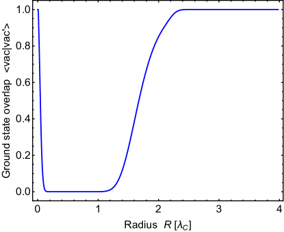
Figure 1: The value of the ground state overlap $\langle\mbox{vac}|\mbox{vac}^{\prime}\rangle$ as a function of radius $R$ (in units of $\lambda_{C}=2\pi/m_{A}=2\pi/(g\,v)$) according to the result in Eq. (47). We have set $g=0.3$ and $\theta_{0}=\pi/4$ here.

Case (a) is that of an ordinary global theory, obtained by sending the gauge coupling $g$ to zero. In this limit $\lambda_{C}\to\infty$, guaranteeing that any finite size sphere trivially satisfies $\lambda_{C}\gg R$. We see that the overlap goes to zero as an exponential in $R^{2}$. This is not as fast as an exponential fall off with volume $V\sim R^{3}$, but is still rather fast. Hence this recovers the well known idea that in an un-gauged field theory, with a global shift symmetry $\theta({\bf x})\to\theta({\bf x})+\theta_{0}$, there is an orthogonal set of vacua labelled by different values of $\langle\theta\rangle=\theta_{0}$ in the large volume limit; which is SSB.

On the other hand, case (b) is that of an ordinary gauge theory with finite gauge coupling $g$. For $W$ and $Z$ bosons in the Standard Model, the Compton wavelength is $\lambda_{C}\sim 10^{-17}$ m. So as long as one is considering spatial regions of size much bigger than $10^{-17}$ m, which is usually the case, then we are in this regime. Here the behavior is radically different. Instead of the overlap wave-functional approaching zero exponentially fast, it approaches one exponentially fast. This means that in the large volume regime, all these wave-functionals are in fact the same. This means there is only a single unique vacuum and no SSB.

We note that the overlap result in Eq. (47) provides a smooth interpolation between these limiting cases. There is at least one situation in which this full result may be important. Instead of heavy $W$ and $Z$ bosons, consider the photon itself. Now it is likely that the photon is strictly massless, but we do not know for sure. A claimed observational bound on the photon mass is $m_{\gamma}\lesssim 10^{-26}$ eV from galactic magnetic fields Goldhaber:2008xy (though the validity of this bound can be debated Adelberger:2003qx). Suppose the photon does indeed have a non-zero mass near this upper bound. This corresponds to a very large Compton wavelength of $\lambda_{C}\sim$ kpc. So if we are interested in physics on scales much larger than $\sim$ kpc, then there is only a unique vacuum (right region of Fig. 1). However, if we focus on physics on scales $\sim$ kpc, then there is effectively many degenerate vacua (middle-left region of Fig. 1). This is similar to the case of having an ultra-light scalar, where depending on the regime of interest, either it is sitting at its true unique vacuum or it may be displaced away from its true vacuum and could be sitting at one of many other effectively degenerate vacua.

V Real or Redundant Transformation?

Above we showed that at finite gauge coupling, there is no SSB in the large volume regime. We can understand this further by re-examining the kernel $M(r)$ that determines the ground state wave-functional. Since the physics at large volume is controlled by small wave-numbers, we can gain some understanding by Taylor expanding the factor $k^{2}/\omega_{k}$ around $k=0$ as

$${k^{2}\over\omega_{k}}={k^{2}\over m_{A}}-{k^{4}\over 2\,m_{A}^{3}}+\ldots.$$ (51)

By interchanging the order of summation and integration, we can readily compute $M(r)$ as a series expansion. The $n^{th}$ term will be proportional to the $2n^{th}$ derivative of the delta-function, i.e.,

$$M(r)=-{v^{2}\over m_{A}}\left[\nabla^{2}\delta^{3}({\bf r})+{\nabla^{4}\delta^{3}({\bf r})\over 2\,m_{A}^{2}}+\ldots\right].$$ (52)

This is related to the above exact result for the kernel; since the kernel is a modified Bessel function, it is large near $r\to 0$, but is exponentially small as $r\to\infty$, which is similar to the structure of the delta-function. By inserting this into the wave-functional in Eq. (36), integrating by parts, and integrating over ${\bf x}^{\prime}$ using the delta-function, we obtain

$$\Psi_{L}(\theta)\propto\exp\left[-{v^{2}\over 2\,m_{A}}\int d^{3}x\left[(\nabla\theta)^{2}-{(\nabla^{2}\theta)^{2}\over 2\,m_{A}^{2}}+\ldots\right]\right].$$ (53)

We have implicitly taken the box size to infinity here in order to integrate by parts and throw away all boundary terms.

In this limit we see that the wave-functional is really only a function of $\nabla\theta$ and not $\theta$. Therefore it is trivially invariant under the transformation $\theta({\bf x})\to\theta({\bf x})+\theta_{0}$. This indicates that such transformation are really just pure gauge transformations (redundancies) in the gauged Higgs phase, even though they are real (global) transformations in the regular phase and in the un-gauged Higgs phase.

In fact we can understand this further by returning to the classical Lagrangian density for the longitudinal modes Eq. (24). Again let us operate in Coulomb gauge $A^{L}=0$. Then let us re-write the Lagrangian density back in position space. Since there are complicated powers of wavenumber $k$, we need to utilize some formal operations involving inverse powers of Laplacians, etc, as follows

$$\mathcal{L}_{L}={v^{2}\over 2}\nabla\dot{\theta}{1\over-\nabla^{2}+g^{2}\,v^{2}}\nabla\dot{\theta}-{v^{2}\over 2}(\nabla\theta)^{2}.$$ (54)

This is indeed a peculiar looking Lagrangian for a scalar field, which we now analyze.

Firstly, note that in the limit in which we send the gauge coupling to zero, we recover the standard Lagrangian of a massless scalar field

$$\mathcal{L}_{L}\to{v^{2}\over 2}\dot{\theta}^{2}-{v^{2}\over 2}(\nabla\theta)^{2},\,\,\,\,\,\mbox{as}\,\,\,\,\,g\to 0.$$ (55)

since the spatial derivatives in the first term of Eq. (54) formally cancels out. In this Lagrangian with $g\to 0$ there is obviously an ordinary global shift symmetry $\theta({\bf x})\to\theta({\bf x})+\theta_{0}$ that is real and physical. It is associated with the existence of a massless boson, by the Goldstone theorem.

On the other hand, for finite gauge coupling, the Lagrangian density in Eq. (54) is rather different. Its radical departure from that of an ordinary massless scalar arises from the coupling to the gauge field and then solving and re-inserting for $A^{0}$. If we focus on low momenta, or small gradients, compared to the spin 1 particle’s mass, we can Taylor expand in $|\nabla {}^2|\ll g{}^{2}v{}^2=m{}_A{}^{2}asfollows\text{(56)Equation 5656LL=v22mA2[(∇˙θ)2-(∇2˙θ)2mA2+…]-v22(∇θ)2.}WenowseethattheLagrangiandensityistriviallyinvariantunder\theta (x)\to \theta (x)+\theta {}_{0}sinceeverytermisonlyafunctionof\nabla \theta .InfacttheLagrangiandensityisinvariantunderamuchlargersetoftransformations\theta (x)\to \theta (x)+f(t),wheref(t)isanarbitraryfunctionoftime.Suchtransformationsarenotphysical,butareinfactpureredundancies.Thisisdirectlyconnectedtotheabovegroundstatewave-functionalbeingalsoonlyafunctionof\nabla \theta atfinitegaugecoupling,andbeingmappedintoitselfunderashiftin\theta .\text{VIsection VIVI§VIVISpectrum}Infactwecanunderstandthebehaviorofthelongitudinalmodemuchmoredirectlybysimplypassingtoacanonicallynormalizedfield.Wecandothisinanygauge,soletusnowgobacktoageneralgauge,anddefinethegaugeinvariantvariable\text{(57)Equation 5757θc(x,t)≡∫d3k(2π)3gALk(t)+kθk(t)ωke-ik⋅x.}Thisnewvariable\theta {}_{c}isdescribedbythemanifestlyLorentzinvariant(asitisgaugeinvariant)Lagrangiandensity\text{(58)Equation 5858LL=v2[12˙θc2-12(∇θc)2-12g2v2θc2],}foranyvalueofthegaugecouplingg.Itisnowcleartoseethatitisonlyinthelimitinwhichwetakeg=0doweobtainaphysicalshiftsymmetry\theta {}_c(x)\to \theta {}_c(x)+\theta {}_0.FurthermorefromEq.(\text{<a href="\#S6.E57" title="In V Real or Redundant Transformation? ‣ Counting of States in Higgs Theories" class="ltx\_ref ltx\_font\_italic"><span class="ltx\_text ltx\_ref\_tag">57</span></a>})wenotethatitisonlyinthislimitthat\theta {}_c=\theta .Otherwisethecanonicallynormalizedfield\theta {}_{c}isverydifferentfrom\theta .Fornon-zerogaugecoupling,thefield\theta {}_{c}hasamassgv.Thisisofcoursethemassofthelongitudinal(andtransverse)modesofthemassivespin1particle.Thisshowsexplicitlythatfornon-zerogaugecouplingthereisonlyauniquevacuumat\theta {}_c=0.Ifthegaugecouplingisverysmall,andwefocusonscalesRmuchlessthantheComptonwavelengthoftheparticle,thereiseffectivelyasetofdegeneratevacua,aswediscussedinSection\text{<a href="\#S4" title="IV Number of Vacua ‣ Counting of States in Higgs Theories" class="ltx\_ref ltx\_font\_italic"><span class="ltx\_text ltx\_ref\_tag">IV</span></a>}.Thekeyideathenisthatinthegauged-Higgstheorythedegeneracyoftheglobaltheoryhasbeenlifted,leavingauniquevacuum.Wecanseeadirectconnectionbetweenthesetofstatesintheglobalcaseandthegaugecase.WehaveillustratedafewofthelowlyingenergylevelsinFig.\text{<span class="ltx\_ref ltx\_missing\_label ltx\_font\_italic ltx\_ref\_self">LABEL:FigureSpectrumMassless</span>}.Thebluerepresentsstatesofzeromomentum,theredrepresentsstateswiththelowestallowednon-zeromomentumk=2\pi /L,andthegreenrepresentsstatesofthesecondlowestallowednon-zeromomentumk=4\pi /L.Solidbluecurverepresentstheinitialvacuum.Dashedrepresentsaddingaparticleofzeromomentum.Dottedrepresentsaddinganotherparticleofzeromomentum.Thereisaone-to-onemappingbetweenthestatesoftheglobalandgaugecases.SoitisimportanttonotethatthereasonthereisonlyoneuniquevacuuminthegaugecaseisnotbecausewehavesimplydeclaredallthevacuatobeequalandreducedthesizeoftheHilbertspacebyhand.InfactthesizeoftheHilbertspaceinthetwocasesisinsomesensethesame(weshallreturntothisinSection\text{<span class="ltx\_ref ltx\_missing\_label ltx\_font\_italic ltx\_ref\_self">LABEL:PathIntegralMeasure</span>}).Itissimplythattheeigen-spectrumhasbeenradicallyalteredduetointerestingdynamics.\text{Figure 2Figure 22Figure 22Afewofthelowlyingenergylevelso}$