Optimal designs for frequentist model averaging

Abstract

We consider the problem of designing experiments for the estimation of a target in regression analysis if there is uncertainty about the parametric form of the regression function. A new optimality criterion is proposed, which minimizes the asymptotic mean squared error of the frequentist model averaging estimate by the choice of an experimental design. Necessary conditions for the optimal solution of a locally and Bayesian optimal design problem are established. The results are illustrated in several examples and it is demonstrated that Bayesian optimal designs can yield a reduction of the mean squared error of the model averaging estimator up to $45\%$.

Keywords: Model selection, model averaging, local misspecification, model uncertainty, optimal design, Bayesian optimal deigns

1 Introduction

It is well known that a carefully designed experiment can improve the statistical inference in regression analysis substantially. Optimal design of experiments is the more efficient the more knowledge about the underlying regression model is available and an impressive theory has been developed to construct optimal designs under the assumption of a “given” regression model [see, for example, the monographs of Pukelsheim, (2006), Atkinson et al., (2007) and Fedorov and Leonov, (2013)]. On the other hand, model selection is an important step in any data analysis and these references also partially discuss the problem of constructing efficient designs to address model uncertainty in the design of experiment. Because of its importance this problem has a long history. Early work dates back to Box and Hill, (1967); Stigler, (1971); Atkinson and Fedorov, (1975) who determined optimal designs for model discrimination by - roughly speaking - maximizing the power of a test between competing regression models [see also Ucinski and Bogacka, (2005); López-Fidalgo et al., (2007); Wiens, (2009); Dette and Titoff, (2009) or Tommasi and López-Fidalgo, (2010) for some more recent references]. A different line of research in this context was initiated by Läuter, (1974) who proposed a criterion based on a product of the determinants of the information matrices in the various models under consideration, which yields efficient designs for all models under consideration. This criterion has been used successfully by Dette, (1990) to determine efficient designs for a class of polynomial regression models and by Biedermann et al., (2006) to construct efficient designs for binary response models, when there is uncertainty about the form of the link function. As these criteria do not reflect model discrimination, Zen and Tsai, (2002); Atkinson, (2008); Tommasi, (2009) considered a mixture of Läuter-type and discrimination criteria to construct efficient designs for model discrimination and parameter estimation. An alternative concept to robust designs with respect to misspecified models consists in the minimization of the maximal mean squared error calculated over a class of misspecified models with respect to the design under consideration [see Wiens, (2015) for an overview]. Several authors have worked on this problem and we mention exemplarily Wiens and Xu, (2008) who derive robust prediction and extrapolation designs or Konstantinou et al., (2017) who analyze robust designs under local alternatives for survival trials. This list of references is by no means complete and there exist many more papers on this subject. However, a common feature in most of the literature consists in the fact that either (at least implicitly) the designs are constructed under the assumption that model selection is performed by hypotheses testing or designs are determined with “good” properties for a class of competing models.

On the other hand there exists an enormous amount of literature to perform statistical inference under model uncertainty, which - to our best knowledge - has not been discussed in the context of optimal experimental design. One possibility is to select an adequate model from a set of candidate models and numerous model selection criteria have been developed for this purpose [see monographs of Burnham and Anderson, (2002), Konishi and Kitagawa, (2008) and Claeskens and Hjort, (2008) among others]. These procedures are widely used and have the advantage to deliver a single model for the statistical analysis, which make them very attractive for practitoners. However, there exists a well known post-selection problem in this approach because estimators chosen after model selection behave usually like mixtures of many potential estimators. For example, if $\mu$ is a parameter of interest in a regression model (such as a prediction at a particular point, the area under the curve or a specific quantile of the regression model) it is known that selecting a single model and ignoring the uncertainty resulting from the selection process may give confidence intervals for $\mu$ with coverage probability smaller than the nominal value, see for example Chapter 7 in Claeskens and Hjort, (2008) for a mathematical treatment or Bornkamp, (2015) for a high-level discussion of this phenomenon.

As an alternative several authors proposed to smooth estimators for the parameter $\mu$ across several models, rather than choosing a specific model from the class under consideration and performing the estimation in the selected model. This approach takes the additional estimator variability caused by model uncertainty adequately into account and has been discussed intensively in the Bayesian community, where it is known as “Bayesian model averaging” [see the tutorial of Hoeting et al., (1999) among many others]. Hjort and Claeskens, (2003) pointed out several problems with this approach. In particular, they mentioned the difficulties to specify prior probabilities for a class of models and the problem of mixing together many conflicting prior opinions in the statistical analysis. As an alternative these authors proposed a non-Bayesian approach, which they call “frequentist model averaging” and developed asymptotic theory for their method. There exists evidence that model averaging improves the estimation efficiency [see Breiman, (1996) or Raftery and Zheng, (2003)], and recently, Schorning et al., (2016) demonstrated the superiority of model averaging about estimation after model selection by an information criterion in the context of dose response models. These results have recently been confirmed by Aoki et al., (2017) and Buatois et al., (2018) in the context of nonlinear mixed effect models.

The present paper is devoted to the construction of optimal designs if parameters of interest are estimated under model uncertainty via frequentist model averaging. Section 2 gives a brief review on model averaging and states the asymptotic properties of this approach under local alternatives. The asymptotic properties are used in Section 3 to define new optimality criteria, which directly reflect the goal of model averaging. Roughly speaking, an optimal design for model averaging estimation minimizes the asymptotic mean squared error of the model averaging estimator under local alternatives. In Section 4 we present a numerical study comparing the optimal designs for model averaging estimation with commonly used designs and demonstrate that the new designs yield substantially more precise estimates. Further simulation results which demonstrate that our findings are representative can be found in Section 6.2. Finally, the proofs of the theoretical results are given in Section 6.1.

2 Model Averaging under local misspecification

Model averaging is a common technique to estimate a parameter of interest, say $\mu$, under model uncertainty. Roughly speaking this estimate is a weighted average of the estimates in the competing models under consideration, where different choices for the weights have been proposed in the literature [see for example Wassermann, (2000) or Hansen, (2007) for Bayesian and non-Bayesian model averaging methods]. In this section we briefly describe this concept and the corresponding asymptotic theory in the present context, such that the results can be used to construct optimal designs for model averaging estimation. The results follow more or less from the statements in Hjort and Claeskens, (2003) and Claeskens and Hjort, (2008) and - although we use a slightly different notation - any details regarding their derivation are omitted for the sake of brevity.

We assume that $k$ different experimental conditions, say $x_{1},\ldots,x_{k}$, are chosen in the design space $\mathcal{X}$, and that at each experimental condition $x_{i}$ one can observe $n_{i}$ responses, say $y_{i1},\ldots,y_{in_{i}}$ $(i=1,...,k)$. We also assume that for each $i=1,\ldots,k$ the responses $y_{i1},\ldots,y_{in_{i}}$ at experimental condition $x_{i}$ are realizations of independent identically (real valued) random variables $Y_{i1},\ldots,Y_{in_{i}}$ with unknown density $f_{\text{true}}(\cdot|x_{i})$. Therefore the total sample size is given by $n=\sum_{i=1}^{k}n_{i}$ and the experimental design problem consists in the choice of $k$ (number of different experimental conditions), $x_{1},\ldots,x_{k}$ (the experimental conditions) and the choice of $n_{1},\ldots,n_{k}$ (the numbers $n_{i}$ of observations taken at each $x_{i}$), such that the model averaging estimate is most efficient.

To measure efficiency and to compare different experimental designs we will use asymptotic arguments and consider the case $\lim_{n\to\infty}\frac{n_{i}}{n}=\xi_{i}\in(0,1)$ for $i=1,\ldots,k$. As common in optimal design theory we collect this information in the matrix

$$\xi=\left\{\begin{array}[]{ccc}x_{1}&\dots&x_{k}\\ \xi_{1}&\dots&\xi_{k}\end{array}\right\}.$$ (2.1)

Following Claeskens and Hjort, (2008) we assume that $f_{\text{true}}(\cdot|x)$ is contained in a set, say $\mathcal{S}$, of parametric candidate densities which is constructed as follows. The first candidate density in $\mathcal{S}$ is given by a parametric density $f_{\text{wide}}(y|x,\theta,\gamma)$, where the form of $f_{\text{wide}}$ is assumed to be known, $\theta=(\theta_{1},\ldots,\theta_{p})\in\Theta$ and $\gamma=(\gamma_{1},\ldots,\gamma_{q})\in\Gamma$ denote the unknown parameters, which vary in a compact parameter space, say $\Theta\times\Gamma\subset\mathbb{R}^{p}\times\mathbb{R}^{q}$. The second candidate density is given by the parametric density $f_{\text{narrow}}(y|x,\theta)=f_{\text{wide}}(y|x,\theta,\gamma_{0})$, which is obtained by fixing the parameter value $\gamma$ to a pre-specified (known) value $\gamma_{0}\in\Gamma$. Throughout the paper, we will call $f_{\text{wide}}(y|x,\theta,\gamma)$ the wide density (model) and $f_{\text{narrow}}(y|x,\theta)$ the narrow density (model), respectively. Additional candidate models are obtained by choosing certain submodels between the wide density $f_{\text{wide}}(y|x,\theta,\gamma)$ and the narrow density $f_{\text{narrow}}(y|x,\theta)$. More precisely, for a chosen subset $S\subset\{1,\ldots,q\}$ of indices with cardinality $|S|$, we introduce the projection matrices $\pi_{S}\in\mathbb{R}^{|S|\times q}$ and $\pi_{S^{c}}\in\mathbb{R}^{|S^{c}|\times q}$ which map a $q$-dimensional vector to its components corresponding to indices in $S$ and $S^{c}$, respectively. Using the abbreviations $\gamma_{S}=\pi_{S}\gamma$ and $\gamma_{0,S^{c}}=\pi_{S^{c}}\gamma_{0}$, we define the candidate density $f_{S}(y|x,\theta,\gamma_{S})$ by

$$f_{S}(y|x,\theta,\gamma_{S})=f_{\text{wide}}(y|x,\theta,\gamma_{S},\gamma_{0,S^{c}}).$$ (2.2)

Consequently, for the density $f_{S}(y|x,\theta,\gamma_{S})$ the components of $\gamma$ with indices in $S^{c}=\{1,\ldots,q\}\setminus S$ are fixed to the corresponding components of $\gamma_{0}$, while the components with indices in $S$ are considered as unknown parameters. Note that $f_{\text{narrow}}=f_{\emptyset}$, $f_{\text{wide}}=f_{\{1,\ldots q\}}$ and that in the most general case there are $2^{q}$ possible candidate densities. As we might not be interested in all possible submodels we assume that the competing models are defined by different sets $S_{1},\ldots,S_{r}\subset\{1,\ldots,q\}$ (for some $r\in\{1,\ldots,2^{q}\}$). Thus the class $\mathcal{S}$ of candidate models is given by

$$\mathcal{S}=\{f_{S_{1}}(y|x,\theta,\gamma_{S_{1}}),\ldots,f_{S_{r}}(y|x,\theta,\gamma_{S_{r}})\}~{}.$$ (2.3)

Following Hjort and Claeskens, (2003), we consider local deviations throughout the paper and assume that the “true” density is given by

$$f_{\text{true},n}(y|x)=f_{\text{wide}}\bigl{(}y|x,\theta_{0},\gamma_{0}+\frac{\delta}{\sqrt{n}}\bigr{)},$$ (2.4)

where the “true” parameter values are given by $\theta_{0}\in\Theta$ and $\gamma_{0}+\tfrac{\delta}{\sqrt{n}}\in\Gamma$. Note that the “true” density is given by the wide density with a varying value of $\gamma$ which differs from $\gamma_{0}$ through the perturbation term $\tfrac{\delta}{\sqrt{n}}$. Thus, for $n$ tending to infinity, it approximates the narrow density $f_{\text{narrow}}(y|x,\theta_{0})$.

Example 2.1

Consider the case, where $f_{\text{wide}}(y|x,\theta,\gamma)=f_{S_{4}}(y|x,\theta,\gamma)$ is a normal density with variance $\sigma^{2}$ and mean function

$$\eta_{S_{4}}(x,\vartheta,\gamma)=\gamma_{1}+\vartheta_{1}\frac{x^{\gamma_{2}}}{x^{\gamma_{2}}+\vartheta_{2}^{\gamma_{2}}},$$ (2.5)

where $\theta^{T}=(\sigma^{2},\vartheta_{1},\vartheta_{2})$, $\gamma^{T}=(\gamma_{1},\gamma_{2})$ and the explanatory variable $x$ varies in an interval, say $[a,b]$. This model is the well known sigmoid Emax model and has numerous applications in modelling the dependence of biochemical or pharmacological responses on concentration [see Goutelle et al., (2008) for an overview]. The sigmoid Emax model is especially popular for describing dose-response relationships in drug development [see MacDougall, (2006) among many others]. The parameters in (2.5) have a concrete interpretation: $\gamma_{1}$ is used to model a Placebo-effect, $\vartheta_{1}$ denotes the maximum effect of $x$ (relative to placebo) and $\vartheta_{2}$ is the value of $x$ which produces half of the maximum effect. The so-called Hill parameter $\gamma_{2}$ characterizes the slope of the mean function $\eta$. The parameter $\theta$ is included in every candidate model, whereas for the narrow model the components are fixed as $\gamma_{0}=(0,1)^{T}$. Consequently, the narrow candidate model is a normal density with mean

$$\eta_{S_{1}}(x,\vartheta)=\frac{\vartheta_{1}x}{x+\vartheta_{2}}$$ (2.6)

and variance $\sigma^{2}$. In this case, $\eta_{S_{1}}$ is the frequently used Michaelis Menten function, which is widely utilized to represent an enzyme kinetics reaction, where enzymes bind substrates and turn them into products [see, for example, Cornish-Bowden, (2012)]. The two other candidate models between are obtained by either fixing $\gamma_{1}=0$ or $\gamma_{2}=1$ and the corresponding densities are normal densities with mean functions

$$\eta_{S_{2}}(x,\vartheta,(0,\gamma_{2}))=\vartheta_{1}\frac{x^{\gamma_{2}}}{x^{\gamma_{2}}+\vartheta_{2}^{\gamma_{2}}}~{},~{}~{}\eta_{S_{3}}(x,\vartheta,(\gamma_{1},1))=\gamma_{1}+\vartheta_{1}\frac{x}{x+\vartheta_{2}},$$ (2.7)

respectively. The latter model is the well known Emax model which is sometimes also referred to as the hyperbolic Emax model [see Holford and Sheiner, (1981) and MacDougall, (2006) among others]. Finally, under the local misspecification assumption (2.4) the true density $f_{\text{true},n}(y|x)$ corresponds to a normal distribution with mean

$$\eta_{\text{true},n}(x)=\frac{\delta_{1}}{\sqrt{n}}+\vartheta_{1}\frac{x^{1+{\delta_{2}}/{\sqrt{n}}}}{x^{1+{\delta_{2}}/{\sqrt{n}}}+\vartheta_{2}^{1+{\delta_{2}}/{\sqrt{n}}}}$$

and variance $\sigma^{2}$. Typical functionals $\mu$ of interest are the area under the curve (AUC)

$$\mu(\theta,\gamma)=\int_{\mathcal{C}}\eta(x,\vartheta,\gamma)dx$$ (2.8)

calculated for a given region $\mathcal{C}\subset\mathbb{R}$ or, for a given $\alpha\in(0,1)$, the “quantile” defined by

$$\mu(\vartheta,\gamma)=\inf\Big{\{}x\in{\cal X}~{}\Big{|}~{}\frac{\eta(x,\vartheta,\gamma)-\eta(a,\vartheta,\gamma)}{\eta(b,\vartheta,\gamma)-\eta(a,\vartheta,\gamma)}\geq\alpha\Big{\}}~{}.$$ (2.9)

The value defined in (2.9) is well-known as $ED_{\alpha}$, that is, the effective dose at which $100\times\alpha\%$ of the maximum effect is achieved [see MacDougall, (2006) or Bretz et al., (2008)].

As pointed out at the end of Example 2.1 we are interested in the estimation of a quantity, say $\mu(\theta,\gamma)$, where $\mu:\Theta\times\Gamma\rightarrow\mathbb{R}$ is a differentiable function of the parameter $(\theta,\gamma)$. For this purpose we fix one model $S\in\mathcal{S}$ in the set of candidate models defined in (2.3) and use the estimator $\hat{\mu}_{S}=\mu(\hat{\theta},\hat{\gamma}_{S},\gamma_{0,S^{c}})$, where $(\hat{\theta},\hat{\gamma}_{S})\in\mathbb{R}^{p+|S|}$ is the maximum-likelihood estimator in model $S$. Under the assumption (2.4) of a local misspecification and the common conditions of regularity [see, for example, Lehmann and Casella, (1998), Chapter 6] it can be shown by adapting the arguments in Hjort and Claeskens, (2003) and Claeskens and Hjort, (2008) to the current situation that the resulting estimator $\hat{\mu}_{S}$ satisfies

$$\sqrt{n}\left(\hat{\mu}_{S}-\mu(\theta_{0},\gamma_{0}+\tfrac{\delta}{\sqrt{n}})\right)\xlongrightarrow{\mathcal{D}}\Lambda_{S}\sim\mathcal{N}(\nu_{S}(\xi),\tau^{2}_{S}(\xi)).$$ (2.10)

Here $\xlongrightarrow{\mathcal{D}}$ denotes weak convergence and $\mathcal{N}(\nu_{S}(\xi),\tau^{2}_{S}(\xi))$ is a normal distribution with variance

$$\tau^{2}_{S}(\xi)=\tau^{2}_{S}(\xi,\theta_{0},\gamma_{0})=c^{T}_{S}J^{-1}_{S}(\xi,\theta_{0},\gamma_{0})c_{S}~{},$$ (2.11)

where $c_{S}$ is the gradient of $\mu$ with respect to $(\theta,\gamma_{S})$, that is,

$$c_{S}=c_{S}(\theta_{0},\gamma_{0,S})=\tfrac{\partial}{\partial(\theta,\gamma_{S})}\mu(\theta,\gamma_{S},\gamma_{0,S^{C}})|_{(\theta,\gamma_{S})=({\theta_{0},\gamma_{0,S}})},$$ (2.12)

and $J_{S}$ the information matrix $J_{S}$ in the candidate model $f_{S}$, that is

$$J_{S}(\xi,\theta_{0},\gamma_{0,S})=\int_{\mathcal{X}}\int\frac{\big{(}\frac{\partial}{\partial(\theta,\gamma_{S})}f_{S}(y|x,\theta_{0},\gamma_{0,S})\big{)}\big{(}\frac{\partial}{\partial(\theta,\gamma_{S})}f_{S}(y|x,\theta_{0},\gamma_{0,S})\big{)}^{T}}{f_{S}(y|x,\theta_{0},\gamma_{0,S})}dy\xi(dx).$$ (2.13)

The mean $\nu_{S}(\xi)$ in (2.10) is of the form

$$\nu_{S}(\xi)=\nu_{S}(\xi,\delta,\theta_{0},\gamma_{0})=c^{T}L_{S}(\xi,\theta_{0},\gamma_{0})\delta~{},$$

where

$$c=c(\theta_{0},\gamma_{0})=\tfrac{\partial}{\partial(\theta,\gamma)}\mu(\theta,\gamma)|_{(\theta,\gamma)=(\theta_{0},\gamma_{0})}$$

is the gradient (with respect to the parameters) in the wide model, the matrix $L_{S}$ is defined by

$$L_{S}(\xi,\theta_{0},\gamma_{0})=\big{(}P_{S}^{T}J_{S}^{-1}(\xi,\theta_{0},\gamma_{0,S})P_{S}J(\xi,\theta_{0},\gamma_{0})-I_{(p+q)\times(p+q)}\big{)}\begin{pmatrix}0_{p\times q}\\ I_{q\times q}\end{pmatrix},$$ (2.14)

the matrices $J_{S}$ and $P_{S}$ are given by (2.13) and

$$P_{S}=\begin{pmatrix}I_{p\times p}&0\\ 0&\pi_{S}\end{pmatrix},$$ (2.15)

respectively, and $J(\xi,\theta_{0},\gamma_{0})$ denotes the information matrix in the wide model $f_{\text{wide}}$.

The frequentist model averaging estimator is now defined by assigning weights $g_{S_{1}},\ldots,g_{S_{r}}$, with $\sum_{i=1}^{r}g_{S_{i}}=1$, to the different candidate models $S_{1},\ldots,S_{r}\in\mathcal{S}$ and defining

$$\hat{\mu}_{\text{mav}}=\sum_{i=1}^{r}g_{S_{i}}\hat{\mu}_{S_{i}},$$ (2.16)

where $\hat{\mu}_{S_{1}},\ldots,\hat{\mu}_{S_{r}}$ are the estimators in the different candidate models $S_{1},\ldots,S_{r}\in\mathcal{S}$. The asymptotic behaviour of the model averaging estimator $\hat{\mu}_{\text{mav}}$ can be derived from Hjort and Claeskens, (2003). In particular, it can be shown that under assumption (2.4) and the standard regularity conditions a standardized version of $\hat{\mu}_{\text{mav}}$ is asymptotically normally distributed, that is

$$\sqrt{n}\left(\hat{\mu}_{\text{mav}}-\mu(\theta_{0},\gamma_{0}+\tfrac{\delta}{\sqrt{n}})\right)\xlongrightarrow{\mathcal{D}}\sum_{i=1}^{r}g_{S_{i}}\Lambda_{S_{i}}\sim\mathcal{N}(\nu(\xi,\delta,\theta_{0},\gamma_{0}),\tau^{2}(\xi,\theta_{0},\gamma_{0}))~{}.$$ (2.17)

Here the mean and variance are given by

$$\nu(\xi,\delta,\theta_{0},\gamma_{0}) = \sum_{i=1}^{r}g_{S_{i}}\nu_{S_{i}}(\xi,\delta,\theta_{0},\gamma_{0}),$$ (2.18)

$$\tau^{2}(\xi,\theta_{0},\gamma_{0}) = \sum_{i=1}^{r}\sum_{j=1}^{r}g_{S_{i}}g_{S_{j}}h^{T}_{S_{i}}(\xi)J(\xi,\theta_{0},\gamma_{0})h_{S_{j}}(\xi),$$ (2.19)

respectively, $J(\xi,\theta_{0},\gamma_{0})$ is the information matrix of the wide model $f_{\text{wide}}$ and the vector $h_{S}(\xi)$ is given by

$$h_{S}(\xi)=P_{S}^{T}J^{-1}_{S}(\xi,\theta_{0},\gamma_{0,S})c_{S},$$ (2.20)

where we used the notation of $c_{S}$, $J_{S}$ and $P_{S}$ introduced (2.12), (2.13) and (2.15). The optimal design criterion for model averaging, which will be proposed in this paper, is based on an asymptotic representation of the mean squared error of the estimate $\hat{\mu}_{\text{mav}}$ derived from (2.17) and will be carefully defined in the following section.

3 An optimality criterion for model averaging estimation

Following Kiefer, (1974) we call the quantity $\xi$ in (2.1) an approximate design on the design space $\mathcal{X}$. This means that the support points ${x_{i}}$ define the distinct dose levels where observations are to be taken and the weights $\xi_{i}$ represent the relative proportion of responses at the corresponding support point $x_{i}$ ($i=1,\ldots,k$). For an approximate design $\xi$ and given total sample size $n$ a rounding procedure is applied to obtain integers $n_{i}$ ($i=1,\ldots,{k})$ from the not necessarily integer valued quantities $\xi_{i}n$ [see, for example Pukelsheim, (2006), Chapter 12], which define the number of observations at $x_{i}$ ($i=1,\ldots,k$).

If the observations are taken according to an approximate design $\xi$ and an appropriate rounding procedure is used such that $n_{i}/n\to\xi_{i}$ as $n\to\infty$, the asymptotic mean squared error of the model averaging estimate $\hat{\mu}_{\text{mav}}$ of the parameter of interest $\mu(\theta_{0},\gamma_{0}+\delta/\sqrt{n})$ can be obtained from the discussion in Section 2, that is

$$\Phi_{\text{mav}}(\xi,g,\delta,\theta_{0},\gamma_{0})=\nu^{2}(\xi,\delta,\theta_{0},\gamma_{0})+\tau^{2}(\xi,\theta_{0},\gamma_{0})\approx n\cdot\text{MSE}(\hat{\mu}_{\text{mav}}),$$ (3.1)

where the variance $\tau^{2}(\xi,\theta_{0},\gamma_{0})$ and the bias $\nu(\xi,\delta,\theta_{0},\gamma_{0})$ are defined in equations (2.18) and (2.19), respectively. Consequently, a “good” design for the model averaging estimate (2.16) should give “small” values of $\Phi_{\text{mav}}$. Therefore, for a given finite set $\mathcal{S}$ of candidate models $f_{S}$ of the form (2.2) and weights $g_{S}$ a design $\xi^{*}$ is called locally optimal design for model averaging estimation of the parameter $\mu$, if it minimizes the function $\Phi_{\text{mav}}(\xi,g,\delta,\theta_{0},\gamma_{0})$ in (3.1) in the class of all approximate designs on $\mathcal{X}$. Here the term “locally” refers to the seminal paper of Chernoff, (1953) on optimal designs for nonlinear regression models.

Locally model averaging optimal designs address uncertainty only with respect to the model $S$ but require prior information for the parameters $\theta_{0},\gamma_{0}$ and $\delta$. While such knowledge might be available in some circumstances [see, for example, Dette et al., (2008) or Bretz et al., (2010)] sophisticated design strategies have been proposed in the literature, which require less precise knowledge about the model parameters, such as sequential, Bayesian or standardized maximin optimality criteria [see Pronzato and Walter, (1985); Chaloner and Verdinelli, (1995) and Dette, (1997) among others]. Any of these methodologies can be used to construct efficient robust designs for model averaging and for the sake of brevity we restrict ourselves to Bayesian optimality criteria.
Here we address the uncertainty with respect to the unknown model parameters by a prior distribution, say $\pi$, on $\Theta\times\Gamma$ and call a design $\xi^{*}$ Bayesian optimal for model averaging estimation of the parameter $\mu$ with respect to the prior $\pi$ if it minimizes the function

$$\Phi^{\pi}_{\text{mav}}(\xi)=\int_{\Theta\times\Gamma}\Phi_{\text{mav}}(\xi,g,\delta,\theta,\gamma)\pi(d\theta,d\gamma),$$ (3.2)

where the function $\Phi_{\text{mav}}$ is defined in (3.1) (we assume throughout this paper that the integral exists).

Locally and Bayesian optimal designs for model averaging have to be calculated numerically in all cases of interest, and we present several examples in Section 4. Next, we state necessary conditions for $\Phi_{\text{mav}}$- and $\Phi_{\text{mav}}^{\pi}$- optimality. The proofs are given in the Section 6.1.

Theorem 3.1

If the design $\xi^{*}$ is a locally optimal design for model averaging estimation of the parameter $\mu$, then the inequality

$$-2\nu(\xi^{*},\delta,\theta_{0},\gamma_{0})D_{1}(\xi^{*},x,\delta,\theta_{0},\gamma_{0})-D_{2}(\xi^{*},x,\theta_{0},\gamma_{0})\leq 0$$ (3.3)

holds for all $x\in\mathcal{X}$, where $\nu(\xi^{*},\delta,\theta_{0},\gamma_{0})$ is defined by (2.18) and the functions $D_{1}$ and $D_{2}$ are given by

$$D_{1}(\xi^{*},x,\delta,\theta_{0},\gamma_{0}) = \sum_{j=1}^{r}g_{S_{j}}c^{T}P_{S_{j}}^{T}J_{S_{j}}^{-1}(\xi^{*},\theta_{0},\gamma_{0,{S_{j}}})\Big{(}P_{S_{j}}J(\xi_{x},\theta_{0},\gamma_{0})$$

$$-J_{S_{j}}(\xi_{x},\theta_{0},\gamma_{0,{S_{j}}})J_{S_{j}}^{-1}(\xi^{*},\theta_{0},\gamma_{0,{S_{j}}})P_{S_{j}}J(\xi^{*},\theta_{0},\gamma_{0})\Big{)}\begin{pmatrix}0_{p}\\ \delta\end{pmatrix},$$

$$D_{2}(\xi^{*},x,\theta_{0},\gamma_{0}) = \sum_{i,j=1}^{r}g_{S_{i}}g_{S_{j}}\left({h}^{T}_{S_{i}}(\xi^{*})\{J(\xi^{*},\theta_{0},\gamma_{0})+J(\xi_{x},\theta_{0},\gamma_{0})\}{h}_{S_{j}}(\xi^{*})\right.$$

$$\left.-2\tilde{h}^{T}_{S_{i}}(\xi^{*},\xi_{x})J(\xi^{*},\theta_{0},\gamma_{0}){h}_{S_{j}}(\xi^{*})\right),$$

where the vector ${h}_{S}(\xi)$ is defined by (2.20), the vector $\tilde{h}_{S}(\xi^{*},\xi)$ by

$$\tilde{h}_{S}(\xi^{*},\xi)=P^{T}_{S}J^{-1}_{S}(\xi^{*},\theta_{0},\gamma_{0,{S}})J_{S}(\xi,\theta_{0},\gamma_{0,{S}})J_{S}^{-1}(\xi^{*},\theta_{0},\gamma_{0,{S}})c_{S},$$

and the information matrix $J_{S}(\xi,\theta_{0},\gamma_{0})$ by (2.13), respectively. The design $\xi_{x}$ denotes the Dirac measure at the point $x\in{\cal X}$.
Moreover, there is equality in (3.3) for every point $x$ in the support of $\xi^{*}$.

Theorem 3.2

If a design $\xi^{*}$ is Bayesian optimal for model averaging estimation of the parameter $\mu$ with respect to the prior $\pi$, then

$$d_{\pi}(x,\xi^{*})=\int_{\Theta\times\Gamma}-2\nu(\xi^{*},\delta,\theta,\gamma)D_{1}(\xi^{*},x,\delta,\theta,\gamma)-D_{2}(\xi^{*},x,\theta,\gamma)\pi(d\theta,d\gamma)\leq 0$$ (3.6)

holds for all $x\in\mathcal{X}$, where the derivatives $D_{1}$ and $D_{2}$ are given by (3.1) and (3.1), respectively.
Moreover, there is equality in (3.6) for every point $x$ in the support of $\xi^{*}$.

The derived conditions of Theorem 3.1 and Theorem 3.2 can be used in the following way: If a numerically calculated design does not satisfy inequality (3.3), it will not be locally optimal for model averaging estimation of the parameter $\mu$ and the search for the optimal design has to be continued. Note that the functions $\Phi_{\text{mav}}$ and $\Phi_{\text{mav}}^{\pi}$ are not convex and therefore sufficient conditions for optimality are not available.

Remark 3.1

Note that Hjort and Claeskens, (2003) also consider model averaging using random weights $g_{S_{1}}(Y_{n}),\ldots,g_{S_{r}}(Y_{n})$ depending on the data $Y_{n}=(Y_{11},\ldots,Y_{1n_{1}},\ldots,Y_{kn_{k}})$ in the definition of the estimator $\hat{\mu}_{\text{mav}}$ in (2.16). Typical examples are smooth AIC-weights

$$g^{{\footnotesize\mbox{smAIC}}}_{S_{j}}(Y_{n})=\frac{\exp(\tfrac{1}{2}\mbox{AIC}(S_{j}|Y_{n}))}{\sum_{i=1}^{r}\exp(\tfrac{1}{2}\mbox{AIC}(S_{i}|Y_{n}))}.$$ (3.7)

which are based on the AIC-scores

$$\mbox{AIC}(S_{i}|Y_{n})=2\ell_{S_{i}}(\hat{\theta},\hat{\gamma}_{S_{i}})-2d_{S_{i}},$$

where $\ell_{S_{i}}(\hat{\theta},\hat{\gamma}_{S_{i}})$ denotes the log-likelihood function of model $S_{i}$ evaluated in the maximum likelihood estimator $(\hat{\theta},\hat{\gamma}_{S_{i}})$ and $d_{S_{i}}$ is the number of parameters to be estimated in model $S_{i}$ ($i=1,\ldots,r$) [see Claeskens and Hjort, (2008), Chapter 2]. Moreover, the estimator of the target $\mu$ which is based on model selection by AIC can also be rewritten in terms of a model averaging estimator by using random weights of the form

$$g^{{\footnotesize\mbox{AIC}}}_{S_{j}}(Y_{n})=I\{S_{j}=S_{{\footnotesize\mbox{AIC}}}\},$$ (3.8)

where $I\{A\}$ is the indicator function of the set $A$ and $S_{{\footnotesize\mbox{AIC}}}$ denotes the model with the greatest AIC-score among the candidate models. For further choices of model averaging weights see for example Buckland et al., (1997), Hjort and Claeskens, (2003) or Hansen, (2007). In general, the case of random weights in model averaging estimation is more difficult to handle and in general the asymptotic distribution is not normal [see Claeskens and Hjort, (2008), p. 196]. As a consequence an explicit calculation of the asymptotic bias and variance is not available.

From the design perspective it therefore seems to be reasonable to consider the case of fixed weights, for which the asymptotic properties of model averaging estimation under local misspecification are well understood and determine efficient designs for this estimation technique. Moreover, we also demonstrate in Section 4 and in the appendix (see Section 6) that model averaging estimation with fixed weights often shows a better performance than model averaging with smooth AIC-weights and that the optimal designs derived under the assumption of fixed weights also improve the current state of the art for model averaging using random weights.

4 Optimal designs for model averaging

In this section, we investigate the performance of optimal designs for model averaging estimation of a parameter $\mu$. For this purpose, we consider several examples from the literature, and compare the Bayesian optimal designs for model averaging estimation of a parameter $\mu$ with commonly used uniform designs by means of a simulation study. Thoughout this paper we use the cobyla algorithm for the minimization of the criterion $\Phi^{\pi}_{\text{mav}}(\xi)$ defined in (3.2) [see Powell, (1994) for details].

4.1 Estimation of the ED_α in the sigmoid Emax model

We consider the situation introduced in Example 2.1, where the underlying density is a normal distribution with variance $\sigma^{2}$ and different regression functions are under consideration for the mean. More precisely, the set $\mathcal{S}$ contains $r=4$ candidate models which are defined by the different mean functions (2.5), (2.6) and (2.7), respectively. The parameter of interest $\mu$ is the $\text{ED}_{0.6}$ defined in (2.9), which is estimated by an appropriate model averaging estimator. The design space is given by the interval $\mathcal{X}=[0,8]$ and we assume that $n=150$ observations can be taken in the experiment.
We determine a Bayesian optimal design for model averaging estimation of the $\mbox{ED}_{0.6}$. As the Emax model is linear in the parameters ${\vartheta_{1}}$ and ${\gamma_{1}}$, the optimality criterion does not depend on ${\vartheta_{1}}$ and ${\gamma_{1}}$ and no prior information is required for these parameters. For the parameters $(\vartheta_{2},\gamma_{2})$ we choose independent uniform priors $\pi_{\vartheta_{2}}$ and $\pi_{\gamma_{2}}$ on the sets $\{0.79,1.79,2.79\}$ and $\{1,2,3\}$, respectively, and the variance ${\sigma^{2}}$ is fixed as $\sigma_{0}^{2}=4.5$ (note that one can choose a prior for $\sigma^{2}$ as well). Finally, under the local misspecification assumption we set $\delta$ such that $\delta/\sqrt{n}=\delta/\sqrt{150}=(0.1,1)^{T}$.
We first consider equal weights for the model averaging estimator, that is $g_{S_{i}}=0.25$, $i=1,\ldots,4$. The Bayesian optimal design for model averaging estimation of the $\mbox{ED}_{0.6}$ is given by

$$\xi^{*}_{A}=\left\{\begin{array}[]{ccccc}0&0.819&1.665&2.669&8\\ 0.105&0.138&0.199&0.273&0.285\end{array}\right\},$$ (4.3)

and satisfies the necessary condition of optimality in Theorem 3.2 [see the left panel of Figure 1]. Note that the design $\xi_{A}^{*}$ defined by (4.3) would not be optimal if the inequality was not satisfied.

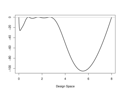
(a)

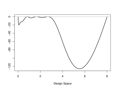
(b)

Figure 1: The function $d_{\pi}$ in (3.6) evaluated for the design $\xi^{*}_{A}$ in (4.3) (left panel) and the design $\xi^{*}_{B}$ in (4.13) (right panel).

In order to investigate the properties of the different designs for model averaging estimation we have conducted a simulation study, where we compare the Bayesian optimal design (4.3) for model averaging estimation of the $\text{ED}_{0.6}$ with two uniform designs

$$\xi_{1} = \left\{\begin{array}[]{ccccc}0&2&4&6&8\\ ^{1}/_{5}&{}^{1}/_{5}&{}^{1}/_{5}&{}^{1}/_{5}&{}^{1}/_{5}\end{array}\right\}~{},$$ (4.6)

$$\xi_{2} = \left\{\begin{array}[]{ccccccccc}0&1&2&3&4&5&6&7&8\\ ^{1}/_{9}&{}^{1}/_{9}&{}^{1}/_{9}&{}^{1}/_{9}&{}^{1}/_{9}&{}^{1}/_{9}&{}^{1}/_{9}&{}^{1}/_{9}&{}^{1}/_{9}\end{array}\right\},$$ (4.9)

which are quite popular in the presence of model uncertainty [see Schorning et al., (2016) and Bornkamp et al., (2007)]. Note that the design $\xi_{1}$ is a uniform design with the same number of support points as the optimal design in (4.3), whereas the design $\xi_{2}$ is a uniform design with more support points. Moreover, we also provide a comparison with two estimators commonly used in practice, namely the model averaging estimator based on smooth AIC-weights defined in (3.7) and the estimator in the model chosen by AIC model selection, which is obtained as a model averaging estimator (2.16) using the weights in (3.8). For these estimators we also used observations taken according to the designs $\xi_{A}^{*}$, $\xi_{1}$ and $\xi_{2}$. As the approximate designs cannot be implemented directly for $n=150$ observations a rounding procedure [see, for example Pukelsheim, (2006), Chapter 12] is applied to determine the number $n_{i}$ of observations taken at $x_{i}$ such that we have in total $\sum_{i=1}^{k}n_{i}=150$ observations. For example, the implemented design obtained from the Bayesian optimal design $\xi_{A}^{*}$ for model averaging estimation of the $\text{ED}_{0.6}$ uses $n_{1}=16$, $n_{2}=21$, $n_{3}=30$, $n_{4}=40$ and $n_{5}=43$ observations at the points $0$, $0.819$, $1.165$, $2.669$ and $8$, respectively, and implementable versions of the designs $\xi_{1}$ and $\xi_{2}$ are obtained similarly.
All results presented here are based on $1000$ simulations runs generating in each run $150$ observations of the form

$$y_{ij}^{(l)}=\gamma_{1}+\vartheta_{1}\frac{x_{i}^{\gamma_{2}}}{x_{i}^{\gamma_{2}}+\vartheta_{2}^{\gamma_{2}}}+\sigma\varepsilon_{ij}^{(l)},i=1,\ldots,k,j=1,\ldots,n_{i},$$ (4.10)

for the different designs, where the $\varepsilon_{ij}^{(l)}$ are independent standard normal distributed random variables and different combinations of the “true” parameter $(\vartheta^{T},\gamma^{T})=(\vartheta_{1},\vartheta_{2},\gamma_{1},\gamma_{2})$ in (4.10) are investigated whereas $\sigma^{2}=4.5$ is fixed. In the following discussion we will restrict ourselves to presenting results for the parameters $(\vartheta_{1},\vartheta_{2})=(1.81,0.79)$, $(\gamma_{1},\gamma_{2})=(0.1,2)$. Note that this is the parameter combination under local misspecification assumption for $\theta_{0}=(4.5,1.81,0.79)^{T}$, $\gamma_{0}=(0,1)^{T}$ and $\delta/\sqrt{150}=(0.1,1)^{T}$. Further simulation results for other parameter combinations can be found in Section 6.2.1.

	estimation method
design	fixed weights	smooth AIC-weights	model selection
$\xi_{A}^{*}$	0.355	0.508	0.596
$\xi_{1}$	0.810	0.913	1.017
$\xi_{2}$	0.637	0.846	0.994

Table 1: The mean squared error of the model averaging estimators with weights $g_{S_{i}}=0.25$, $i=1,\ldots,4$ (left column), with the smooth AIC-weights (3.7) (middle column) and the estimator based on model-selection (right column). The different rows correspond to different designs. First row: Bayesian optimal design $\xi^{*}_{A}$ for model averaging estimation of the $\text{ED}_{0.6}$ defined in (4.3). Middle row: uniform design $\xi_{1}$ defined in (4.6). Third row: uniform design $\xi_{2}$ defined in (4.9).

In each simulation run, the parameter $\mu=\mbox{ED}_{0.6}$ is estimated by model averaging using the different designs and the mean squared error is calculated from all $1000$ simulation runs. More precisely, if $\hat{\mu}^{(l)}_{\text{mav}}$ is the model averaging estimator for the parameter of interest $\mu=\mbox{ED}_{0.6}$ based on the observations $y^{(l)}_{11},\ldots,y^{(l)}_{kn_{k}}$ from model (4.10) with the design $\xi$, its mean squared error is given by

$$\text{MSE}(\xi)=\frac{1}{1000}\sum_{l=1}^{1000}\left(\hat{\mu}_{\text{mav}}^{(l)}-\mu_{true}\right)^{2},$$

where $\mu_{true}$ is the $\mbox{ED}_{0.6}$ in the “true” sigmoid Emax model (4.10) with parameters $(\vartheta^{T},\gamma^{T})=(1.81,0.79,0.1,2)$. The simulated mean squared error of the model averaging estimator with fixed weights $g_{S_{i}}=0.25$, $i=1,\ldots,4$ for the different designs $\xi^{*}_{A}$, $\xi_{1}$ and $\xi_{2}$ is shown in the left column of Table 1. The middle column of this table shows the mean squared error of the model averaging estimator with the smooth AIC-weights in (3.7), while the right column gives the corresponding results for the weights in (3.8), that is estimation of the $\mbox{ED}_{0.6}$ in the model identified by the AIC for the different designs. The numbers printed in boldface in each column correspond to the smallest mean squared error obtained from the three designs.
We observe that model averaging always yields a smaller mean squared error than estimation in the model identified by the AIC. For example, if the design $\xi^{*}_{A}$ is used, the mean squared error of the estimator based on model selection is $0.596$, whereas it is $0.355$ and $0.508$ for the model averaging estimator using fixed weights and smooth AIC-weights, respectively (see the first row in Table 1). The situation for the non-optimal uniform designs is similar. These results (and also further simulation results presented in Section 6.2.1) coincide with the findings of Schorning et al., (2016), Aoki et al., (2017) and Buatois et al., (2018) and indicate that model averaging usually yields more precise estimates of the target than estimators based on model selection. Moreover, model averaging estimation with fixed weights shows a substantially better performance than the model averaging estimator with data driven weights. Note that Wagner and Hlouskova, (2015) observed a similar effect in the context of principal components augmented regressions.

	estimation method
design	fixed weights	smooth AIC-weights	model selection
$\xi_{B}^{*}$	0.476	0.502	0.582
$\xi_{1}$	0.915	0.900	1.014
$\xi_{2}$	0.869	0.949	1.067

Table 2: The mean squared error of the model averaging estimators with weights $g_{S_{1}}=0.1$, $g_{S_{2}}=0.1$, $g_{S_{3}}=0.3$ and $g_{S_{4}}=0.5$ (left column), with the smooth AIC-weights (3.7) (middle column) and the estimator based on model-selection (right column). The different rows correspond to different designs. First row: Bayesian optimal design $\xi^{*}_{B}$ for model averaging estimation of the $\text{ED}_{0.6}$ defined in (4.13). Middle row: uniform design $\xi_{1}$ defined in (4.6). Third row: uniform design $\xi_{2}$ defined in (4.9).

Compared to the uniform designs $\xi_{1}$ and $\xi_{2}$ the optimal design $\xi^{*}_{A}$ in (4.3) yields a reduction of the mean squared error by $56\%$ and $44\%$ for model averaging estimation with fixed weights. Moreover, this design also reduces the mean squared error of model averaging estimation with smooth AIC-weights (by $44\%$ and $40\%$) and for estimation in the model identified by the AIC (by $41\%$ and $40\%$).
As a further example we consider the model averaging estimator (2.16) of the parameter $\mbox{ED}_{0.6}$ for the four models in Example 2.1 with non-equal weights, that is $g_{S_{1}}=0.1$ , $g_{S_{2}}=0.1$, $g_{S_{3}}=0.3$ and $g_{S_{4}}=0.5$. The Bayesian optimal design for model averaging estimation of the $\text{ED}_{0.6}$ is then given by

$$\xi^{*}_{B}=\left\{\begin{array}[]{ccccc}0&0.809&1.665&2.691&8\\ 0.152&0.120&0.175&0.279&0.274\end{array}\right\}.$$ (4.13)

The necessary condition is depicted in the right panel of Figure 1. A comparison of the designs $\xi^{*}_{A}$ and $\xi^{*}_{B}$ in (4.3) and (4.13) shows that the support points are similar, but that there appear substantial differences in the weights.
In the simulation study of this model averaging estimator we consider the same parameters as in the previous example. The corresponding results can be found in Table 2 and show a similar but less pronounced picture as for the model averaging estimator with uniform weights. Model averaging always shows a better performance than estimation in the model selected by the AIC (improvement between $10\%$ and $19\%$ using fixed weights and between $11\%$ and $14\%$ using smooth AIC-weights). Moreover, for the designs $\xi_{B}^{*}$ and $\xi_{2}$ we observe an improvement when using fixed weights instead of smooth AIC-weights for model averaging, but for the design $\xi_{1}$ there is in fact no improvement. A comparison of the results in Table 1 and 2 shows that for all designs non-uniform weights for model averaging estimation yield a larger mean squared error than uniform weights.
The Bayesian optimal design $\xi^{*}_{B}$ for model averaging estimation of the $\text{ED}_{0.6}$ improves the designs $\xi_{1}$ and $\xi_{2}$ by $48\%$ and $45\%$, respectively, if model averaging with fixed (non-uniform weights) is used, and by $43\%-47\%$ for model averaging estimation with smooth AIC-weights and estimation in the model selected by the AIC.
Simulation results for further parameter combinations in the sigmoid Emax model can be found in Table 5 and 6 in Section 6.2.1. These results show a very similar picture as described in the previous paragraphs. We observe that in all considered scenarios model averaging estimation yields a smaller simulated mean squared error than estimation in a model identified by the AIC, independently of the design and parameters under consideration. Bayesian optimal designs for model averaging estimation of the $\text{ED}_{0.6}$ yield a substantially more precise estimation than the uniform designs in almost all cases. We refer to Section 6.2.1 for more details.

4.2 Estimation of the AUC in the logistic regression model

In this section we consider the logistic regression model

$$\eta_{S_{4}}(x,\vartheta,\gamma)=\gamma_{1}+\frac{\vartheta_{1}}{1+\exp[(\vartheta_{2}-x)/\gamma_{2}]},~{}x\geq 0$$ (4.14)

which is frequently used in dose-response modeling or modeling population growth [see, for example, Zwietering et al., (1990)]. This means we consider a normal distribution with variance $\sigma^{2}$ and mean (function) given by (4.14). The design space is given by $\mathcal{X}=[0,8]$ and we are interested in the estimation of the area under the curve (AUC) defined in (2.8), where the region $\mathcal{C}$ and the design space $\mathcal{X}$ coincide. In model (4.14) the value $\eta(0,\vartheta,\gamma)$ is the Placebo-effect, $\vartheta_{1}$ denotes the maximum effect (relative to placebo) of the drug and $\vartheta_{2}>0$ is the dose which produces half of the maximum effect. The parameter $\gamma_{2}$ characterizes the slope of the mean function $\eta$. We assume that the parameter $\theta=(\sigma^{2},\vartheta_{1},\vartheta_{2})^{T}$ is included in every candidate model, whereas the components of the parameter $\gamma=(\gamma_{1},\gamma_{2})^{T}$ can be fixed to the corresponding components of $\gamma_{0}=(0,1)^{T}$, such that there are $r=4$ competing models in the candidate set $\mathcal{S}$, that is

$$\eta_{S_{1}}(x,\vartheta) =\frac{\vartheta_{1}}{1+\exp[(\vartheta_{2}-x)]},$$ (4.15)

$$\eta_{S_{2}}(x,\vartheta,(0,\gamma_{2})^{T}) =\frac{\vartheta_{1}}{1+\exp[(\vartheta_{2}-x)/\gamma_{2}]},$$ (4.16)

$$\eta_{S_{3}}(x,\vartheta,(\gamma_{1},1)^{T}) =\gamma_{1}+\frac{\vartheta_{1}}{1+\exp[(\vartheta_{2}-x)]}.$$ (4.17)

and $\eta_{S_{4}}$ defined by (4.14). As the parameters $\gamma_{1}$ and $\vartheta_{1}$ appear linear in the model only the prior distributions for $\gamma_{2}$ and $\vartheta_{2}$ have to be specified, which are chosen as independent uniform priors supported on the sets $\{3,4,5\}$ and $\{5/6,1,7/6\}$, respectively. The variance $\sigma^{2}$ is fixed as $\sigma_{0}^{2}=4.5$ and $\delta$ is chosen such that $\delta^{T}/\sqrt{150}=(0.015,-1/6)$.
The Bayesian optimal design for model averaging estimation of the AUC with equal weights $g_{S_{i}}=0.25,i=1,\ldots,4,$ has been calculated numerically and is given by

$$\xi^{*}_{C}=\left\{\begin{array}[]{ccccc}0&2.585&4.332&5.419&8\\ 0.094&0.258&0.239&0.204&0.206\end{array}\right\}.$$ (4.20)

The performance of the different designs is again evaluated by means of a simulation study generating data from the model

$$y_{ij}^{(l)}=\gamma_{1}+\frac{\vartheta_{1}}{1+\exp[(\vartheta_{2}-x)/\gamma_{2}]}+\sigma\varepsilon_{ij}^{(l)},i=1,...,k,j=1,...,n_{i},$$ (4.21)

where $\varepsilon_{ij}^{(l)}$ are standard normal distributed random variables and $n=\sum_{i=1}^{k}n_{i}=150$ observations can be taken. We focus on the case $\vartheta^{T}=(\vartheta_{1},\vartheta_{2})=(-1.73,4)$, $\gamma^{T}=(0.015,0.833)$ and $\sigma^{2}=4.5$ which corresponds to a local misspecification, where $\theta_{0}^{T}=(4.5,-1.73,4),\ \gamma_{0}^{T}=(0,1)$ and $\delta^{T}/\sqrt{150}=(0.015,-1/6)$. Further results for other parameter choices show a similar picture and are given and discussed in Section 6.2.2 of the appendix.

	estimation method
design	fixed weights	smooth AIC	model selection
$\xi^{*}_{C}$	1.659	1.880	2.074
$\xi_{1}$	1.961	2.080	2.196
$\xi_{2}$	1.687	1.763	1.838

Table 3: The mean squared error of the model averaging estimators with weights $g_{S_{i}}=0.25$, $i=1,\ldots,4$ (left column), with the smooth AIC-weights (3.7) (middle column) and the estimator based on model-selection (right column). The different rows correspond to different designs. First row: Bayesian optimal design $\xi^{*}_{C}$ for model averaging estimation of the AUC defined in (4.20). Middle row: uniform design $\xi_{1}$ defined in (4.6). Third row: uniform design $\xi_{2}$ defined in (4.9).

The mean squared error of the model averaging estimator with equal weights $g_{S_{i}}=0.25$ ($i=1,\ldots,4$) for the different designs is given in the left column of Table 3, while the middle and right column show the corresponding results for the model averaging estimator with smooth AIC-weights and the estimator based on model selection, respectively. We observe again that model averaging improves the estimation of the target AUC in all cases under consideration. For fixed weights this improvement varies between $8\%$ and $20\%$ (depending on the design), while the improvement achieved by model averaging with smooth AIC-weights varies between $4\%$ and $9\%$. The model averaging estimator with fixed (equal) weights performs substantially better than the procedure with smooth AIC-weights.
In the case of fixed weights the Bayesian optimal design $\xi_{C}^{*}$ for model averaging estimation of the AUC yields a $15\%$ improvement of the the uniform design $\xi_{1}$ but only a $2\%$ improvement of the design $\xi_{2}$. On the other hand, if model averaging estimates with smooth AIC-weights or model selection weights are used, the uniform design $\xi_{2}$ shows the best performance. This observation can be explained by the fact that the design $\xi_{C}^{*}$ has not been constructed for this purpose. Consequently, although this design performs very well in many cases, it cannot be guaranteed that the design $\xi_{C}^{*}$ is close to the optimal design for model averaging estimation of the AUC with smooth AIC-weights or for the estimation in a model selected by the AIC. Nevertheless, model averaging with fixed weights and the corresponding Bayesian optimal design yields the smallest mean squared error in all considered scenarios.

	estimation method
design	fixed weights	smooth AIC	model selection
$\xi^{*}_{D}$	1.764	1.723	1.835
$\xi_{1}$	2.059	2.041	2.129
$\xi_{2}$	1.841	1.801	1.883

Table 4: The mean squared error of the model averaging estimators with weights $g_{S_{1}}=0.1$, $g_{S_{2}}=0.1$, $g_{S_{3}}=0.1$ and $g_{S_{4}}=0.7$ (left column), with the smooth AIC-weights (3.7) (middle column) and the estimator based on model-selection (right column). The different rows correspond to different designs. First row: Bayesian optimal design $\xi^{*}_{D}$ for model averaging estimation of the AUC defined in (4.24). Middle row: uniform design $\xi_{1}$ defined in (4.6). Third row: uniform design $\xi_{2}$ defined in (4.9).

Next we consider a model averaging estimator with (non-uniform) weights $g_{S_{1}}=0.1$, $g_{S_{2}}=0.1$, $g_{S_{3}}=0.1$, and $g_{S_{4}}=0.7$ for the models (4.15), (4.16), (4.17) and (4.14), respectively. The corresponding Bayesian optimal design for model averaging estimation of the AUC with these weights is is given by

$$\xi^{*}_{D}=\left\{\begin{array}[]{ccccc}0&2.418&4.259&5.777&8\\ 0.122&0.284&0.197&0.253&0.145\end{array}\right\}.$$ (4.24)

The mean squared error of the model averaging estimators for different designs is given in the left column of Table 4, where we use the same parameters as in the previous example. The middle and right column show the simulated mean squared error for model averaging estimation with smooth AIC-weights and the estimator based on model selection, respectively. We observe a similar behaviour as described in Section 4.1: model averaging performs better than model selection but in this situation model averaging based on smooth AIC-weights results in a slightly smaller mean squared error than model averaging based on fixed weights (the estimator with fixed weights yields an increase of the mean squared error of about $2\%$). For all three estimators the mean squared error from the Bayesian optimal design $\xi_{D}^{*}$ defined in (4.24) is smaller than the ones obtained from the designs $\xi_{1}$ and $\xi_{2}$.
Further simulation results using other parameter combinations can be found in Table 7 (model averaging estimator with equal weights) and Table 8 (model averaging estimator with non-uniform weights) in the appendix and show a similar picture as described in the previous paragraphs. For example, model averaging shows a better performance than estimation in a model identified by the AIC, independently of the design under consideration. In most cases the Bayesian optimal design for model averaging estimation of the AUC yields a substantial improvement compared to the uniform designs, even when it is used for model averaging with smooth AIC-weights or for estimation after model selection (see Section 6.2.2 for more details).

5 Conclusions

In this paper we studied the problem of constructing efficient designs for parametric regression if model averaging is used to estimate a target under model uncertainty. We have developed a new optimality criterion which determines a design such that the asymptotic mean squared error of the estimator of the target (under local deviation from the assumed model) becomes minimal by the choice of the experimental design. The results are illustrated by means of a simulation study in the problem of estimating the effective dose and the area under the curve. The optimal designs yield a substantial reduction of the mean squared error of the frequentist model averaging estimate.
The optimal designs constructed for model averaging with fixed weights also improve model averaging estimates with smooth AIC-weights and estimates in a model selected by an information type criterion. However, it remains an open and very challenging question for future research to determine optimal designs for estimation methods of this type. The asymptotic distribution of these estimators is complicated and has to be simulated in general for each design under consideration, which is computationally very demanding. A further interesting direction of future research in this context consists in the construction and investigation of adaptive designs, which proceed in several steps, updating the information about the models and their parameters sequentially.

Acknowledgements This work has been supported in part by the Collaborative Research Center “Statistical modeling of nonlinear dynamic processes” (SFB 823, Teilprojekt C2, T1) of the German Research Foundation (DFG) and by a grant from the National Institute of General Medical Sciences of the National Institutes of Health under Award Number R01GM107639. The content is solely the responsibility of the authors and does not necessarily represent the official views of the National Institutes of Health.

6 Appendix

6.1 Proof of Theorem 3.1 and Theorem 3.2

Theorem 3.1 is a special case of Theorem 3.2, since the Bayesian model averaging optimality criterion reduces to the local model averaging optimality criterion with respect to the parameter $(\theta_{0}^{T},\gamma_{0}^{T},\delta^{T})$ by choosing a one-point prior. Following the arguments in Pukelsheim, (2006)[Chapter 11] and assuming that integration and differentiation are interchangeable, a Bayesian optimal design $\xi^{*}$ for model averaging estimation of the parameter $\mu$ satisfies the inequality

$$-D\Phi_{\text{mav}}(\xi^{*})(\xi_{x}-\xi^{*})=-\int_{\Theta\times\Gamma}D\Phi_{\text{mav}}(\xi^{*},g,\delta,\theta,\gamma)(\xi_{x}-\xi^{*})\pi(d\theta,d\gamma)\leq 0$$ (A.1)

for all $x\in\mathcal{X}$, where $D\Phi_{\text{mav}}(\xi^{*},g,\delta,\theta_{0},\gamma_{0})(\xi_{x}-\xi^{*})$ denotes the directional derivative of the function $\Phi_{\text{mav}}$ evaluated in the optimal design $\xi^{*}$ in direction $\xi_{x}-\xi^{*}$ and $\xi_{x}$ denotes the Dirac measure at the point $x\in{\cal X}$. Note that in the particular case of the model averaging optimality criterion, the corresponding function $\Phi_{\text{mav}}^{\pi}(\xi)$ is not convex and therefore the necessary condition in (A.1) is not sufficient.
We now calculate an explicit expression of the derivative using the chain rule

$$D\Phi_{\text{mav}}(\xi^{*},g,\delta,\theta,\gamma)(\xi_{x}-\xi^{*})=2\nu(\xi^{*})D_{1}(\xi^{*},x,\delta,\theta,\gamma)+D_{2}(\xi^{*},x,\theta,\gamma),$$ (A.2)

where $D_{1}(\xi^{*},x,\delta,\theta,\gamma)$ is the directional derivative of the bias function $\nu$ defined by (2.18) and $D_{2}(\xi^{*},x,\theta,\gamma)$ is the directional derivative of the variance function $\tau^{2}$ defined by (2.19).
We consider these derivatives separately starting with $D_{1}(\xi^{*},x,\delta,\theta,\gamma)$, for which we obtain

$$D_{1}(\xi^{*},x,\delta,\theta,\gamma)=\sum_{j=1}^{r}g_{S_{j}}c^{T}DL_{S_{j}}(\xi^{*},\theta,\gamma)(\xi_{x}-\xi^{*})\delta,$$ (A.3)

where $DL_{S_{j}}(\xi^{*},\theta,\gamma)(\xi_{x}-\xi^{*})$ denotes the derivative of the function $L_{S_{j}}$ defined in (2.14) and is therefore given by

$$\begin{split}DL_{S_{j}}(\xi^{*},\theta,\gamma)(\xi_{x}-\xi^{*})=&P^{T}_{S_{j}}J_{S_{j}}^{-1}(\xi^{*},\theta,\gamma_{S_{j}})\left(P_{S_{j}}J(\xi_{x},\theta,\gamma)\right.\\ &\left.-J_{S_{j}}(\xi_{x},\theta,\gamma_{S_{j}})J_{S_{j}}^{-1}(\xi^{*},\theta,\gamma_{S_{j}})P_{S_{j}}J(\xi^{*},\theta,\gamma)\right)\begin{pmatrix}0_{p\times q}\\ I_{q\times q}\end{pmatrix}.\end{split}$$ (A.4)

Here we used that the derivative of the inverse of the information matrix, $J^{-1}_{S}(\xi^{*})$, in direction $\xi^{*}-\xi_{x}$ is of the form

$$DJ_{S}^{-1}(\xi^{*},\theta,\gamma_{S})(\xi_{x}-\xi^{*})=J_{S}^{-1}(\xi^{*},\theta,\gamma_{S})-J_{S}^{-1}(\xi^{*},\theta,\gamma_{S})J_{S}(\xi_{x},\theta,\gamma_{S})J_{S}^{-1}(\xi^{*},\theta,\gamma_{S}),$$ (A.5)

for an arbitrary $S\subset\{1,\ldots,q\}$. Combining (A.3) and (A.4) follows in the representation of $D_{1}$ given in (3.1).
The derivative $D_{2}(\xi^{*},x,\theta,\gamma)$ is of the form

$$\begin{split}D_{2}(\xi^{*},x,\theta,\gamma)=\sum_{i,j=1}^{r}g_{S_{i}}g_{S_{j}}&\left(2Dh^{T}_{S_{i}}(\xi^{*})(\xi_{x}-\xi^{*})J(\xi^{*},\theta,\gamma)h_{S_{j}}(\xi^{*})\right.\\ &\left.+h_{S_{i}}^{T}(\xi^{*})\{J(\xi^{*},\theta,\gamma)+J(\xi_{x},\theta,\gamma)\}h_{S_{j}}(\xi^{*})\right),\end{split}$$ (A.6)

where $Dh_{S}(\xi^{*})(\xi_{x}-\xi^{*})$ denotes the derivative of $h_{S}$ defined by (2.20) for an aribitrary subset $S\subset\{1,\ldots,q\}$. Using (A.5) $Dh_{S}(\xi^{*})(\xi_{x}-\xi^{*})$ is given by

$$Dh_{S}(\xi^{*})(\xi_{x}-\xi^{*})=h_{S}(\xi^{*})-\tilde{h}_{S}(\xi^{*},\xi_{x})$$ (A.7)

where $\tilde{h}_{S}$ is defined by

$$\tilde{h}_{S}(\xi^{*},\xi_{x})=P^{T}_{S}J^{-1}_{S}(\xi^{*},\theta,\gamma_{S})J_{S}(\xi_{x},\theta,\gamma_{S})J_{S}^{-1}(\xi^{*},\theta,\gamma_{S})c_{S}.$$

Combining (A.6) and (A.7) results in the representation of $D_{2}$ given in (3.1). Finally, the necessary condition in (3.3) follows by the combination of (A.1) and (A.2).

To prove that there holds equality in (3.6) for all support points $x$ of the design $\xi^{*}$, assume that there exists at least one support point $x_{0}$ of the design $\xi^{*}$, such that the inequality in (3.6) is strict. Then, we have

$$\int_{\mathcal{X}}\int_{\Theta\times\Gamma}\left(-2\nu(\xi^{*},\delta,\theta,\gamma)D_{1}(\xi^{*},x,\delta,\theta,\gamma)-D_{2}(\xi^{*},x,\theta,\gamma)\right)\pi(d\theta,d\gamma)\xi^{*}(dx)<0.$$

On the other hand, since $\int_{\mathcal{X}}J(\xi_{x},\theta,\gamma)\xi^{*}(dx)=J(\xi^{*},\theta,\gamma)$ and $\int_{\mathcal{X}}\tilde{h}_{S}(\xi^{*},\xi_{x})\xi^{*}(dx)=h_{S}(\xi^{*})$, we have

$$\int_{\mathcal{X}}D_{1}(\xi^{*},x,\delta,\theta,\gamma)\xi^{*}(dx)=0\text{ and }\int_{\mathcal{X}}D_{2}(\xi^{*},x,\theta,\gamma)\xi^{*}(dx)=0,$$

such that

$$\int_{\mathcal{X}} \int_{\Theta\times\Gamma}-2\nu(\xi^{*},\delta,\theta,\gamma)D_{1}(\xi^{*},x,\delta,\theta,\gamma)-D_{2}(\xi^{*},x,\theta,\gamma)\pi(d\theta,d\gamma)\xi^{*}(dx)$$

$$=\int_{\Theta\times\Gamma}\left\{-2\nu(\xi^{*},\delta,\theta,\gamma)\int_{\mathcal{X}}D_{1}(\xi^{*},x,\delta,\theta,\gamma)\xi^{*}(dx)-\int_{\mathcal{X}}D_{2}(\xi^{*},x,\theta,\gamma)\xi^{*}(dx)\right\}\pi(d\theta,d\gamma)=0,$$

which is a contradiction. Consequently, equality in (3.6) must hold whenever $x$ is a support point of the design $\xi^{*}$.

6.2 Additional simulation results

6.2.1 Estimation of the $\text{ED}_{0.6}$

Parameter	design	estimation method
$(\vartheta,\gamma)$		fixed weights	smooth AIC	model selection
	$\xi_{A}^{*}$	0.818	1.065	1.180
(1.81,0.79,0,1)	$\xi_{1}$	1.339	1.526	1.660
	$\xi_{2}$	1.207	1.549	1.791
	$\xi_{A}^{*}$	0.718	0.957	1.059
(1.81,0.79,0.1,1)	$\xi_{1}$	1.238	1.413	1.535
	$\xi_{2}$	1.045	1.406	1.695
	$\xi_{A}^{*}$	0.394	0.533	0.639
(1.81,0.79,0,2)	$\xi_{1}$	0.788	0.823	0.915
	$\xi_{2}$	0.659	0.852	0.975
	$\xi_{A}^{*}$	0.355	0.508	0.596
(1.81,0.79,0.1,2)	$\xi_{1}$	0.810	0.913	1.017
	$\xi_{2}$	0.637	0.846	0.994
	$\xi_{A}^{*}$	0.732	0.953	1.103
(1.81,1.79,0,2)	$\xi_{1}$	1.374	1.570	1.767
	$\xi_{2}$	1.119	1.437	1.660
	$\xi_{A}^{*}$	0.777	1.121	1.453
(1.81,1.79,0.1,2)	$\xi_{1}$	1.166	1.384	1.532
	$\xi_{2}$	0.985	1.222	1.415
	$\xi_{A}^{*}$	0.449	0.513	0.623
(1.81,1.79,0,3)	$\xi_{1}$	0.988	1.144	1.250
	$\xi_{2}$	0.762	0.908	1.049
	$\xi_{A}^{*}$	0.464	0.598	0.713
(1.81,1.79,0.1,3)	$\xi_{1}$	0.932	1.182	1.314
	$\xi_{2}$	0.724	0.892	1.061

Table 5: The mean squared error of the model averaging estimators of the $\text{ED}_{0.6}$ with weights $g_{S_{i}}=0.25,i=1,\ldots,4$ (left column), with the smooth AIC-weights (3.7) (middle column) and the estimator based on model-selection (right column). The different rows correspond to different parameter combinations. Within each parameter combination the different rows correspond to different designs. First row: Bayesian optimal design $\xi^{*}_{A}$ for model averaging estimation of the $\text{ED}_{0.6}$ defined in (4.3). Middle row: uniform design $\xi_{1}$ defined in (4.6). Third row: uniform design $\xi_{2}$ defined in (4.9).

Parameter	design	estimation method
$(\vartheta,\gamma)$		fixed weights	smooth AIC	model selection
	$\xi_{B}^{*}$	0.864	0.849	1.012
(1.81,0.79,0,1)	$\xi_{1}$	1.504	1.498	1.605
	$\xi_{2}$	1.382	1.450	1.631
	$\xi_{B}^{*}$	0.914	0.937	1.112
(1.81,0.79,0.1,1)	$\xi_{1}$	1.493	1.497	1.613
	$\xi_{2}$	1.306	1.310	1.491
	$\xi_{B}^{*}$	0.540	0.536	0.600
(1.81,0.79,0,2)	$\xi_{1}$	0.967	0.967	1.048
	$\xi_{2}$	0.834	0.861	1.004
	$\xi_{B}^{*}$	0.476	0.502	0.582
(1.81,0.79,0.1,2)	$\xi_{1}$	0.915	0.900	1.014
	$\xi_{2}$	0.869	0.949	1.067
	$\xi_{B}^{*}$	0.904	0.873	1.038
(1.81,1.79,0,2)	$\xi_{1}$	1.292	1.329	1.506
	$\xi_{2}$	1.362	1.338	1.611
	$\xi_{B}^{*}$	0.875	0.931	1.091
(1.81,1.79,0.1,2)	$\xi_{1}$	1.382	1.410	1.573
	$\xi_{2}$	1.350	1.368	1.599
	$\xi_{B}^{*}$	0.516	0.532	0.619
(1.81,1.79,0,3)	$\xi_{1}$	1.129	1.144	1.251
	$\xi_{2}$	0.836	0.813	0.927
	$\xi_{B}^{*}$	0.578	0.560	0.615
(1.81,1.79,0.1,3)	$\xi_{1}$	1.130	1.171	1.304
	$\xi_{2}$	0.800	0.851	1.023

Table 6: The mean squared error of the model averaging estimators of the $\text{ED}_{0.6}$ with weights $g_{S_{1}}=0.1,g_{S_{2}}=0.1,g_{S_{3}}=0.3$ and $g_{S_{4}}=0.5$ (left column), with the smooth AIC-weights (3.7) (middle column) and the estimator based on model-selection (right column). The different rows correspond to different parameter combinations. Within each parameter combination the different rows correspond to different designs. First row: Bayesian optimal design $\xi^{*}_{B}$ for model averaging estimation of the $\text{ED}_{0.6}$ defined in (4.13). Middle row: uniform design $\xi_{1}$ defined in (4.6). Third row: uniform design $\xi_{2}$ defined in (4.9).

In this section we present further simulation results for the estimation of the $\text{ED}_{0.6}$ in the sigmoid Emax model. Data is generated from the model (4.10) where $n=150$ observations are taken according to the designs $\xi_{A}^{*}$, $\xi_{B}^{*}$, $\xi_{1}$ and $\xi_{2}$ defined in Section 4.1. Different parameters $(\vartheta,\gamma)$ are considered to demonstrate that the results in Section 4.1 are representative. The simulated mean squared error for the model averaging estimates of the $\text{ED}_{0.6}$ can be found in Table 5 (uniform weights $g_{S_{i}}=0.25,i=1,\ldots,4$) and Table 6 (non-uniform weights $g_{S_{1}}=0.1,g_{S_{2}}=0.1,g_{S_{3}}=0.3$ and $g_{S_{4}}=0.5$). In the left and middle column we display the results for the model averaging estimator of the $\text{ED}_{0.6}$ with fixed weights and with smooth AIC-weights, respectively, while the right column shows the results for estimation of the $\text{ED}_{0.6}$ in the model selected via AIC.
We observe from Table 5 that model averaging estimation always yields a smaller mean squared error than estimation after model selection via AIC. Model averaging estimation with fixed weights results in a reduction of the mean squared error by $14\%$-$47\%$ whereas smooth AIC-weights reduce the mean squared error by $7\%$-$23\%$. Moreover, model averaging with fixed weights shows a better performance than model averaging with data driven smooth AIC-weights. Table 6 shows similar results for model averaging estimation with non-uniform weights, but the difference between model averaging estimation with fixed weights and data driven weights is less substantial. Moreover, there are also a few parameter combinations where using non-uniform fixed weights yields a slight increase of the mean squared error (about $1-3\%$) compared to smooth AIC-weights.
Next we compare the optimal designs $\xi_{A}^{*}$ and $\xi_{B}^{*}$ with the uniform designs $\xi_{1}$ and $\xi_{2}$ which yield a reduction of the mean squared error of the model averaging estimator of the $\text{ED}_{0.6}$ with fixed weights by $21\%$-$56\%$ and by $28\%$-$54\%$, respectively. For model averaging estimation with smooth AIC-weights the optimal designs $\xi_{A}^{*}$ and $\xi_{B}^{*}$ reduce the mean squared error by $8\%$-$55\%$ and $28\%$-$53\%$, respectively. Finally, for estimation of the $\text{ED}_{0.6}$ in the model identified by the AIC the optimal designs reduce the mean squared error in almost all considered cases.

6.2.2 Estimation of the AUC

Parameter	design	estimation method
$(\vartheta,\gamma)$		fixed weights	smooth AIC	model selection
	$\xi^{*}$	1.559	1.741	1.871
(-1.73,4,0,1)	$\xi_{1}$	1.886	1.963	2.030
	$\xi_{2}$	1.880	1.959	2.042
	$\xi^{*}$	1.503	1.658	1.802
(-1.73,4,0.015,1)	$\xi_{1}$	2.060	2.140	2.222
	$\xi_{2}$	1.831	1.917	1.981
	$\xi^{*}$	1.630	1.825	1.986
(-1.73,4,0,0.833)	$\xi_{1}$	2.042	2.139	2.230
	$\xi_{2}$	1.681	1.811	1.883
	$\xi^{*}$	1.659	1.880	2.074
(-1.73,4,0.015,0.833)	$\xi_{1}$	1.961	2.080	2.196
	$\xi_{2}$	1.687	1.763	1.838
	$\xi^{*}$	1.442	1.637	1.762
(-1.73,5,0,0.833)	$\xi_{1}$	1.671	1.815	1.925
	$\xi_{2}$	1.659	1.846	1.996
	$\xi^{*}$	1.517	1.773	1.953
(-1.73,5,0.015,0.833)	$\xi_{1}$	1.690	1.820	1.924
	$\xi_{2}$	1.629	1.764	1.884
	$\xi^{*}$	1.389	1.688	1.873
(-1.73,5,0,0.667)	$\xi_{1}$	1.672	1.823	1.955
	$\xi_{2}$	1.511	1.691	1.807
	$\xi^{*}$	1.421	1.687	1.839
(-1.73,5,0.015,0.667)	$\xi_{1}$	1.649	1.870	2.040
	$\xi_{2}$	1.626	1.792	1.907

Table 7: The mean squared error of the model averaging estimators of the AUC with weights $g_{S_{i}}=0.25,i=1,\ldots,4$ (left column), with the smooth AIC-weights (3.7) (middle column) and the estimator based on model-selection (right column). The different rows correspond to different parameter combinations. Within each parameter combination the different rows correspond to different designs. First row: Bayesian optimal design $\xi^{*}_{C}$ for model averaging estimation of the AUC defined in (4.20). Middle row: uniform design $\xi_{1}$ defined in (4.6). Third row: uniform design $\xi_{2}$ defined in (4.9).

Parameter	design	estimation method
$(\vartheta,\gamma)$		fixed weights	smooth AIC	model selection
	$\xi^{*}$	1.913	1.851	1.956
(-1.73,4,0,1)	$\xi_{1}$	2.159	2.128	2.213
	$\xi_{2}$	1.942	1.918	1.989
	$\xi^{*}$	1.890	1.843	1.951
(-1.73,4,0.015,1)	$\xi_{1}$	2.042	2.018	2.106
	$\xi_{2}$	1.935	1.912	1.959
	$\xi^{*}$	1.662	1.604	1.702
(-1.73,4,0,0.833)	$\xi_{1}$	1.964	1.934	2.025
	$\xi_{2}$	1.832	1.807	1.875
	$\xi^{*}$	1.764	1.723	1.835
(-1.73,4,0.015,0.833)	$\xi_{1}$	2.059	2.041	2.129
	$\xi_{2}$	1.841	1.801	1.883
	$\xi^{*}$	1.863	1.771	1.886
(-1.73,5,0,0.833)	$\xi_{1}$	1.881	1.818	1.930
	$\xi_{2}$	1.842	1.813	1.942
	$\xi^{*}$	1.689	1.617	1.761
(-1.73,5,0.015,0.833)	$\xi_{1}$	2.006	1.944	2.083
	$\xi_{2}$	1.700	1.670	1.815
	$\xi^{*}$	1.671	1.590	1.716
(-1.73,5,0,0.667)	$\xi_{1}$	1.833	1.769	1.925
	$\xi_{2}$	1.818	1.768	1.920
	$\xi^{*}$	1.745	1.665	1.816
(-1.73,5,0.015,0.667)	$\xi_{1}$	1.896	1.824	1.957
	$\xi_{2}$	1.649	1.626	1.779

Table 8: The mean squared error of the model averaging estimators of the AUC with weights $g_{S_{1}}=0.1,g_{S_{2}}=0.1,g_{S_{3}}=0.1$ and $g_{S_{4}}=0.7$ (left column), with the smooth AIC-weights (3.7) (middle column) and the estimator based on model-selection (right column). The different rows correspond to different parameter combinations. Within each parameter combination the different rows correspond to different designs. First row: Bayesian optimal design $\xi^{*}_{D}$ for model averaging estimation of the AUC defined in (4.24). Middle row: uniform design $\xi_{1}$ defined in (4.6). Third row: uniform design $\xi_{2}$ defined in (4.9).

In this section we present further simulation results for model averaging estimation of the AUC in the logistic model. We generate data from the model (4.21) where $n=150$ observations are taken according to the designs $\xi_{1}$ and $\xi_{2}$, $\xi_{C}^{*}$, $\xi_{D}^{*}$ defined in Section 4.2. To validate the findings in Section 4.2 for other choices of the parameter we consider further scenarios for the parameter $(\vartheta,\gamma)$ and simulate the mean squared error of the model averaging estimators of the AUC. The results can be found in Table 7 (uniform weights $g_{S_{i}}=0.25,i=1,\ldots,4$) and Table 8 (non-uniform weights $g_{S_{1}}=0.1,g_{S_{2}}=0.1,g_{S_{3}}=0.1$ and $g_{S_{4}}=0.7$). In the left column of these tables we display the results of the model averaging estimator of the AUC with fixed weights, while the middle and right column show the mean squared error of the model averaging estimator with smooth AIC-weights and the estimator based on model selection, respectively.
As in Section 4.2 we observe that the mean squared error of model averaging estimators is always smaller than the mean squared error of estimators after model selection via AIC (improvement: $7\%$-$26\%$ with uniform weights, $1\%$-$7\%$ with non-uniform weights and $2\%$-$10\%$ with smooth AIC-weights). Model averaging estimation of the AUC with uniform weights yields a reduction of the mean squared error by $4\%$-$18\%$ (depending on the design and parameters) compared to model averaging estimation with smooth AIC-weights [see Table 7]. On the other hand non-uniform weights yield a slight increase of the mean squared error [see Table 8].
We observe from Table 7 that the Bayesian optimal designs improve the uniform designs for model averaging estimation of the AUC with uniform weights in all scenarios under consideration (improvement: $2\%$-$27\%$). For the estimator with non-uniform weights the improvement varies between $1\%$-$16\%$, although there are a few parameter combinations with no improvement [see Table 8]. For model averaging with data driven weights the optimal design $\xi_{C}^{*}$ (constructed for fixed weights) improves the uniform design $\xi_{2}$ in roughly half of the scenarios under consideration and the the Bayesian optimal design $\xi_{D}^{*}$ determined for non-uniform weights performs better than $\xi_{1}$ and $\xi_{2}$ in most cases.

References

- Aoki et al., (2017) Aoki, Y., Röshammar, D., Hamrén, B., and Hooker, A. C. (2017). Model selection and averaging of nonlinear mixed-effect models for robust phase III dose selection. Journal of Pharmacokinetics and Pharmacodynamics, 44(6):581–597.
- Atkinson, (2008) Atkinson, A. C. (2008). -optimum designs for model discrimination and parameter estimation. Journal of Statistical Planning and Inference, 138:56–64.
- Atkinson et al., (2007) Atkinson, A. C., Donev, A., and Randall, T. (2007). Optimum Experimental Designs, with SAS. Oxford University Press, Oxford.
- Atkinson and Fedorov, (1975) Atkinson, A. C. and Fedorov, V. V. (1975). The designs of experiments for discriminating between two rival models. Biometrika, 62:57–70.
- Biedermann et al., (2006) Biedermann, S., Dette, H., and Pepelyshev, A. (2006). Some robust design strategies for percentile estimation in binary response models. Canadian Journal of Statistics, 34:603–622.
- Bornkamp, (2015) Bornkamp, B. (2015). Viewpoint: Model selection uncertainty, pre-specification and model averaging. Pharmaceutical Statistics, 14(2):79–81.
- Bornkamp et al., (2007) Bornkamp, B., Bretz, F., Dmitrienko, A., Enas, G., Gaydos, B., Hsu, C.-H., König, F., Krams, M., Liu, Q., Neuenschwander, B., Parke, T., and Pinheiro, J. (2007). Innovative approaches for designing and analyzing adaptive dose-ranging trials. Journal of Biopharmaceutical Statistics, 17(6):965–995.
- Box and Hill, (1967) Box, G. E. P. and Hill, W. J. (1967). Discrimination among mechanistic models. Technometrics, 9(1):57–71.
- Breiman, (1996) Breiman, L. (1996). Bagging predictors. Machine Learning, 24:123–140.
- Bretz et al., (2010) Bretz, F., Dette, H., and Pinheiro, J. (2010). Practical considerations for optimal designs in clinical dose finding studies. Statistics in Medicine, 29(7-8):731–742.
- Bretz et al., (2008) Bretz, F., Hsu, J., and Pinheiro, J. (2008). Dose finding – a challenge in statistics. Biometrical Journal, 50(4):480–504.
- Buatois et al., (2018) Buatois, S., Ueckert, S., Frey, N., Retout, S., and Mentré, F. (2018). Comparison of model averaging and model selection in dose finding trials analyzed by nonlinear mixed effect models. The AAPS journal, 20:56.
- Buckland et al., (1997) Buckland, S. T., Burnham, K. P., and Augustin, N. H. (1997). Model selection: An integral part of inference. Biometrics, 53(2):603–618.
- Burnham and Anderson, (2002) Burnham, K. P. and Anderson, D. R. (2002). Model Selection and Multimodel Inference: A Practical Information-Theoretic Approach (2nd ed.). Springer-Verlag, New York.
- Chaloner and Verdinelli, (1995) Chaloner, K. and Verdinelli, I. (1995). Bayesian experimental design: A review. Statist. Sci., 10(3):273–304.
- Chernoff, (1953) Chernoff, H. (1953). Locally optimal designs for estimating parameters. Annals of Mathematical Statistics, 24:586–602.
- Claeskens and Hjort, (2008) Claeskens, G. and Hjort, N. L. (2008). Model Selection and Model Averaging. Cambridge University Press.
- Cornish-Bowden, (2012) Cornish-Bowden, A. (2012). Fundamentals of Enzyme Kinetics (4th ed.). Wiley-VCH, Weinheim.
- Dette, (1990) Dette, H. (1990). A generalization of - and -optimal designs in polynomial regression. Annals of Statistics, 18:1784–1805.
- Dette, (1997) Dette, H. (1997). Designing experiments with respect to “standardized” optimality criteria. Journal of the Royal Statistical Society, Ser. B, 59:97–110.
- Dette et al., (2008) Dette, H., Bretz, F., Pepelyshev, A., and Pinheiro, J. C. (2008). Optimal designs for dose finding studies. Journal of the American Statisical Association, 103:1225–1237.
- Dette and Titoff, (2009) Dette, H. and Titoff, S. (2009). Optimal discrimination designs. Ann. Statist., 37(4):2056–2082.
- Fedorov and Leonov, (2013) Fedorov, V. V. and Leonov, S. L. (2013). Optimal Design for Nonlinear Response Models. CRC Press, Boca Raton, FL, USA.
- Goutelle et al., (2008) Goutelle, S., Maurin, M., Rougier, F., Barbaut, X., Bourguignon, L., Ducher, M., and Maire, P. (2008). The hill equation: a review of its capabilities in pharmacological modelling. Fundamental and Clinical Pharmacology, 22:633–648.
- Hansen, (2007) Hansen, B. E. (2007). Least squares model averaging. Econometrica, 75(4):1175–1189.
- Hjort and Claeskens, (2003) Hjort, N. L. and Claeskens, G. (2003). Frequentist Model Average Estimators. Journal of the American Statistical Association, 98(464):879–899.
- Hoeting et al., (1999) Hoeting, J. A., Madigan, D., Raftery, A. E., and Volinsky, C. T. (1999). Bayesian model averaging: a tutorial (with comments by m. clyde, david draper and e. i. george, and a rejoinder by the authors. Statist. Sci., 14(4):382–417.
- Holford and Sheiner, (1981) Holford, N. H. and Sheiner, L. B. (1981). Understanding the dose–effect relationship: Clinical application of pharmacokinetic–pharmacodynamic models. Clinical Pharmacokinetics, 6:429–453.
- Kiefer, (1974) Kiefer, J. (1974). General Equivalence Theory for Optimum Designs (Approximate Theory). The Annals of Statistics, 2(5):849–879.
- Konishi and Kitagawa, (2008) Konishi, S. and Kitagawa, G. (2008). Information Criteria and Statistical Modeling. John Wiley & Sons, New York.
- Konstantinou et al., (2017) Konstantinou, M., Biedermann, S., and Kimber, A. (2017). Model robust designs for survival trials. Computational Statistics & Data Analysis, 113:239 – 250.
- Läuter, (1974) Läuter, E. (1974). Experimental design in a class of models. Math. Operationsforsch. Statist., 5(4 & 5):379–398.
- Lehmann and Casella, (1998) Lehmann, E. and Casella, G. (1998). Theory of Point Estimation. Springer Texts in Statistics. Springer New York.
- López-Fidalgo et al., (2007) López-Fidalgo, J., Tommasi, C., and Trandafir, P. C. (2007). An optimal experimental design criterion for discriminating between non-normal models. Journal of the Royal Statistical Society, Series B, 69:231–242.
- MacDougall, (2006) MacDougall, J. (2006). Analysis of Dose-Response Studies - Model. In Ting, N., editor, Dose Finding in Drug Development, pages 127–145. Springer, New York.
- Powell, (1994) Powell, M. J. D. (1994). A direct search optimization method that models the objective and constraint functions by linear interpolation. In Hennart, J.-P. and Gomez, S., editors, Advances in Optimization and Numerical Analysis, pages 51–67. Dordrecht.
- Pronzato and Walter, (1985) Pronzato, L. and Walter, E. (1985). Robust experimental design via stochastic approximation. Mathematical Biosciences, 75:103–120.
- Pukelsheim, (2006) Pukelsheim, F. (2006). Optimal Design of Experiments. Classics in Applied Mathematics. Society for Industrial and Applied Mathematics. DOI: 10.1137/1.9780898719109.
- Raftery and Zheng, (2003) Raftery, A. and Zheng, Y. (2003). Discussion: Performance of bayesian model averaging. Journal of the American Statistical Association, 98:931–938.
- Schorning et al., (2016) Schorning, K., Bornkamp, B., Bretz, F., and Dette, H. (2016). Model selection versus model averaging in dose finding studies. Statistics in Medicine, 35(22):4021–4040.
- Stigler, (1971) Stigler, S. (1971). Optimal experimental design for polynomial regression. Journal of the American Statistical Association, 66:311–318.
- Tommasi, (2009) Tommasi, C. (2009). Optimal designs for both model discrimination and parameter estimation. Journal of Statistical Planning and Inference, 139:4123–4132.
- Tommasi and López-Fidalgo, (2010) Tommasi, C. and López-Fidalgo, J. (2010). Bayesian optimum designs for discriminating between models with any distribution. Computational Statistics & Data Analysis, 54(1):143–150.
- Ucinski and Bogacka, (2005) Ucinski, D. and Bogacka, B. (2005). -optimum designs for discrimination between two multiresponse dynamic models. Journal of the Royal Statistical Society, Ser. B, 67:3–18.
- Wagner and Hlouskova, (2015) Wagner, M. and Hlouskova, J. (2015). Growth regressions, principal components augmented regressions and frequentist model averaging. Jahrbücher für Nationalökonomie und Statistik, 235(6):642–662.
- Wassermann, (2000) Wassermann, L. (2000). Bayesian model selection and model averaging. Journal of Mathematical Psychology, 44:92–107.
- Wiens, (2015) Wiens, D. (2015). Robustness of design. In Dean, A., Morris, M., Stufken, J., and Bingham, D., editors, Handbook of Design and Analysis of Experiments. CRC press, Boca Raton.
- Wiens, (2009) Wiens, D. P. (2009). Robust discrimination designs. Journal of the Royal Statistical Society, Ser. B, 71(4):805–829.
- Wiens and Xu, (2008) Wiens, D. P. and Xu, X. (2008). Robust prediction and extrapolation designs for misspecified generalized linear regression models. Journal of Statistical Planning and Inference, 138(1):30 – 46. International Conference on Design of Experiments (ICODOE).
- Zen and Tsai, (2002) Zen, M.-M. and Tsai, M.-H. (2002). Some criterion-robust optimal designs for the dual problem of model discrimination and parameter estimation. Sankhya: The Indian Journal of Statistics, 64:322–338.
- Zwietering et al., (1990) Zwietering, M. H., Jöngenburger, I., Rombouts, F. M., and Ried, K. V. (1990). Modeling of the bacterial growth curve. Applied and Environmental Microbiology, 56(6):1875–1881.