Magnon band topology in spin-orbital coupled magnets:
classification and application to $\alpha$-RuCl₃

Abstract

In spite of flourishing studies on the topology of spin waves, a generic framework to classify and compute magnon band topology in non-collinear magnets is still missing. In this work we provide such a theory framework, by mapping an arbitrary linear spin wave into a local free-fermion Hamiltonian with exactly the same spectrum, symmetry implementation and band topology, which allows for a full classification and calculation on any topological properties of magnon bands. We apply this fermionization approach to honeycomb Kitaev magnet $\alpha$-RuCl₃, and show the existence of topologically protected magnon band crossings, and field-induced magnon Chern bands under small magnetic fields.

I Introduction

The discovery of topological insulators revealed a large class of electronic materials, which support symmetry protected surface states as a manifestation of nontrivial bulk topological propertiesHasan and Kane (2010); Qi and Zhang (2011); Chiu et al. (2016); Armitage et al. (2018). The success of topological band theory in electronic systems leads to a natural question: can similar topological phenomena appear in the energy bands of quasiparticle excitations in a bosonic system? Indeed various topological bands and protected surface states have been engineered in mechanicalKane and Lubensky (2014); Lubensky et al. (2015); Huber (2016) and photonic systemsOzawa et al. (2018). Meanwhile, the prevalent family of magnetically ordered materials provide another ideal platform, where the spin wave excitations can realize various topological bands and magnon surface surface states. Although lots of discoveries have been made recentlyChisnell et al. (2015, 2016); Yao et al. (2017); Shindou et al. (2013a, b); Zhang et al. (2013); Lisenkov et al. (2014); Romhányi et al. (2015); Lawler (2016); Kim et al. (2016); Owerre (2016a, b); Li et al. (2016); Attig and Trebst (2017); Laurell and Fiete (2017); Nakata et al. (2017); Li and Hu (2017); Li et al. (2017); Iacocca and Heinonen (2017); Joshi and Schnyder (2017); Hwang et al. (2017); Bao et al. (2018); Joshi (2018) on the topology of spin waves (or magnons), unlike in electronic systems, a systematic framework to understand magnon band topology is still lacking.

In this work, we resolve this issue by establishing an exact mapping between a (bosonic) linear spin wave theory and a (fermionic) free-electron system. This mapping preserves locality and all physical symmetries of the linear spin wave, so that the corresponding pair of linear spin wave (or magnon) and free fermion systems share exactly the same bulk spectrum and band topology. For example, the magnons of a generic spin-orbit coupled magnet are mapped to Bogoliubov quasiparticles in an electronic superconductor. In another more familiar example, magnons in a collinear magnet with $U(1)$ spin conservation are mapped to electrons in an insulator with $U(1)$ charge conservation.

This “fermionization” approach establishes a correspondence between linear spin waves and well-understood free-fermion Hamiltonians, thus allowing us to fully classify and compute band topology of spin wave (or magnon) excitations. To demonstrate its power, we apply this formulation to study magnon band topology in layered honeycomb “Kitaev material” $\alpha$-RuCl₃, where spin-orbit couplings play an important roleRau et al. (2016); Winter et al. (2017a); Hermanns et al. (2018). We show that the zigzag order in $\alpha$-RuCl₃ exhibits symmetry-protected magnon band touchings, and they can be lifted by an external magnetic field, giving rise to magnon Chern bands with chiral magnon edge states. We study the evolution of magnon bands in $\alpha$-RuCl₃ by varying the applied magnetic field, and obtain a phase diagram of magnon band topology as a function of the magnetic field.

II Fermionization and band topology of linear spin waves

In an ordered magnet, spins precess around the direction of the local magnetic field, which is determined by the local moment via the magnetic interaction. The dynamics of a generic linear spin wave (LSW) is determined by the following equation of motion (e.o.m.):

$$-\hskip 1.0pt\mathrm{i}\hskip 1.0pt\frac{\text{d}s_{i}^{\alpha}}{\text{d}t}=\sum_{j,\beta}\big{(}\sigma_{y}\cdot{\bf R}\big{)}_{i\alpha,j\beta}s_{j}^{\beta},\leavevmode\nobreak\ \leavevmode\nobreak\ \leavevmode\nobreak\ \alpha,\beta=x,y$$ (1)

where $\vec{s}_{i}$ denotes the fluctuation of spin ${\bf S}_{i}$ on site $i$ from its ordered moment $\langle{{\bf S}_{i}}\rangle$

$$\vec{s}_{i}={\bf S}_{i}-\langle{{\bf S}_{i}}\rangle$$ (2)

For convenience we have chosen a local coordinate frame where the ordered moment $\langle{{\bf S}_{i}}\rangle$ on every site $i$ points to $\hat{z}$ direction, and Pauli matrices $\vec{\sigma}$ act on the $\alpha=x,y$ indices. As detailed in supplemental materials, the matrix ${\bf R}$ is fully determined by the original spin Hamiltonian and the ordered moments $\{\langle{{\bf S}_{i}}\rangle\}$ of the LSW.

Eq. (1) can be viewed as a Schrodinger equation, where eigenvalues of matrix $\sigma_{y}\cdot{\bf R}$ determine the magnon (or spin wave) spectrum. The fact that ${\bf R}={\bf R}^{\ast}$ is a real matrix implies a “particle-hole symmetry” of the eigenvalues of $\sigma_{y}{\bf R}$: a positive eigenvalue $\omega_{j}>0$ must appear in pair with a negative eigenvalue $-\omega_{j}<0$. In a generic spin-orbit coupled magnet, the “Hamiltonian” matrix $\sigma_{y}\cdot{\bf R}$ is not Hermitian. This roots in the difference between bose and fermi statistics, as compared to a Hermitian Hamiltonian in any free-fermion system.

	Spin wave e.o.m.	Holstein-Primakoff approach	Free fermion systems
Physical problems	$-\hskip 1.0pt\mathrm{i}\hskip 1.0pt\partial_{t}\vec{s}=(\sigma_{y}{\bf R})\cdot\vec{s}$	$\mathcal{H}_{\text{H-P}}=\phi^{\dagger}{\bf H}_{b}\phi$	$\mathcal{H}_{\text{FF}}=\psi^{\dagger}{\bf H}_{f}\psi$
Variables	$\vec{s}=(s_{i}^{x},s_{i}^{y})^{T}$	$\phi=(b_{i},b_{i}^{\dagger})^{T}$	$\psi=\big{(}\frac{f_{i}+f_{i}^{\dagger}}{2},\hskip 1.0pt\mathrm{i}\hskip 1.0pt\frac{f_{i}^{\dagger}-f_{i}}{2}\big{)}^{T}$
“Hamiltonian” matrix	${\bf R}={\bf R}^{\dagger}={\bf R}^{\ast}$	${\bf H}_{b}=U^{\dagger}{\bf R}U$	${\bf H}_{f}=\sqrt{\bf R}\cdot\sigma_{y}\cdot\sqrt{\bf R}$
		$U=e^{\hskip 1.0pt\mathrm{i}\hskip 1.0pt\frac{\pi}{4}(1-\sigma_{z})}e^{\hskip 1.0pt\mathrm{i}\hskip 1.0pt\frac{\pi}{4}\sigma_{y}}$
Diagonalization	$(\sigma_{y}{\bf R})\cdot({\bf B}e^{\hskip 1.0pt\mathrm{i}\hskip 1.0pt\frac{\pi}{4}\sigma_{x}})=$	$(\sigma_{z}{\bf H}_{b})\cdot{\bf W}_{b}=$	${\bf H}_{f}\cdot{\bf W}_{f}=$
of Hamiltonian	$({\bf B}e^{\hskip 1.0pt\mathrm{i}\hskip 1.0pt\frac{\pi}{4}\sigma_{x}})\cdot(\sigma_{z}\otimes\mathbf{\Omega})$	${\bf W}_{b}\cdot(\sigma_{z}\otimes\mathbf{\Omega})$	${\bf W}_{f}\cdot(-\sigma_{z}\otimes\mathbf{\Omega})$
“Particle-hole”	${\bf R}={\bf R}^{\ast}$,	${\bf H}_{b}=\sigma_{x}{\bf H}_{b}^{\ast}\sigma_{x}$,	${\bf H}_{f}^{\ast}=-{\bf H}_{f}$,
symmetry	${\bf B}={\bf B}^{\ast}$.	${\bf W}_{b}^{\ast}=\sigma_{x}{\bf W}_{b}\sigma_{x}$.	${\bf W}_{f}^{\ast}={\bf W}_{f}\sigma_{x}$.
Wavefunction	${\bf B}^{\dagger}\sigma_{y}{\bf B}=\sigma_{y}$	${\bf W}_{b}^{\dagger}\sigma_{z}{\bf W}_{b}=\sigma_{z}$	${\bf W}_{f}^{\dagger}{\bf W}_{f}=1$
normalization
Relation between	${\bf B}_{2N\times 2N}\in Sp(2N,\mathbb{R})$	${\bf W}_{b}=U^{\dagger}{\bf B}U$	${\bf W}_{f}=\sqrt{\bf R}{\bf B}U\mathbf{\Omega}^{-\frac{1}{2}}$
wavefunctions			$=U\sqrt{{\bf H}_{b}}{\bf W}_{b}\mathbf{\Omega}^{-\frac{1}{2}}$
Diagonal form	${\bf R}=\sigma_{y}{\bf B}\mathbf{\Omega}{\bf B}^{\dagger}\sigma_{y}$	${\bf H}_{b}=\sigma_{z}{\bf W}_{b}\mathbf{\Omega}{\bf W}_{b}^{\dagger}\sigma_{z}$	${\bf H}_{f}={\bf W}_{f}(-\sigma_{z}\mathbf{\Omega}){\bf W}_{f}^{\dagger}$
Unitary symmetry $g\in G_{s}$	$[O_{g},{\bf R}]=0,$	$[U^{\dagger}O_{g}U,{\bf H}_{b}]=0,$	$O_{g}{\bf H}_{f}O_{g}^{\dagger}={\bf H}_{f}$
$O_{g}\in Sp(2N,\mathbb{R})$	$[O_{g},\sigma_{y}]=0$	$[U^{\dagger}O_{g}U,\sigma_{z}]=0$
Anti-unitary symmetry $h\in G_{s}$	$[O_{h},{\bf R}]=0,$	$[U^{\dagger}O_{h}U,{\bf H}_{b}]=0,$	$O_{h}{\bf H}_{f}O_{h}^{\dagger}=-{\bf H}_{f}={\bf H}_{f}^{\ast}$
$O_{h}\in SO(2N)$	$\{O_{h},\sigma_{y}\}=0$	$\{U^{\dagger}O_{h}U,\sigma_{z}\}=0$

Table 1: The relation between semiclassical LSW equation of motion (e.o.m.), Holstein-Primakoff boson formalism of LSWs, and the corresponding free-fermion systems with the same spectrum. The “particle-hole symmetry” is a redundancy of the formulation rather than a physical symmetry. We have defined $\mathbf{\Omega}_{i,j}\equiv\delta_{ij}\omega_{j}\geq 0$ as the diagonal matrix of non-negative magnon frequencies, and $U=e^{\hskip 1.0pt\mathrm{i}\hskip 1.0pt\frac{\pi}{4}(1-\sigma_{z})}e^{\hskip 1.0pt\mathrm{i}\hskip 1.0pt\frac{\pi}{4}\sigma_{y}}$ is a unitary rotation in the $\vec{\sigma}$ space satisfying $U^{\ast}=U\sigma_{x}=\sigma_{z}U$. This fermionization map is well defined for gapped magnon spectra with $\det{\bf R}\neq 0$.

To map the LSW into a free-fermion system, the key step is the following similarity transformation:

$${\bf R}^{1/2}\cdot\big{(}\sigma_{y}{\bf R}\big{)}\cdot{\bf R}^{-1/2}=\sqrt{\bf R}\leavevmode\nobreak\ \sigma_{y}\sqrt{\bf R}={\bf H}_{f}$$ (3)

Note that for a generic spin-orbit coupled magnet, the gapped magnon spectrum indicates that matrix ${\bf R}$ is positive-definite and hence its square root is uniquely defined. This “fermionization map” generates a free fermion Hamiltonian ${\bf H}_{f}$ with exactly the same spectrum as the boson Hamiltonian. It’s straightforward to check that ${\bf H}_{f}$ is Hermitian and particle-hole symmetric. Moreover it preserves the same symmetries as the LSW, as shown in TABLE 1. While every gapped LSW system can be mapped to a short-ranged free-fermion model, not all free-fermion Hamiltonians have their LSW counterpart. As proved in Supplemental materials, the ground state for any free-fermion counterpart ${\bf H}_{f}$ of the LSW Hamiltonian ${\bf R}$ must be a trivial product state, since it can always be adiabatically connected to the fermion atomic insulator without closing the gap while preserving the same symmetries. This is consistent with topological triviality of a magnetically-ordered ground state, and rules out the possibility of any zero-energy magnon surface states protected by symmetries.

Although the magnetic ground state at zero energy is topologically trivial, each magnon band can still exhibit nontrivial topology and symmetry-protected surface states at finite energy. Using known K-theory classificationKitaev (2009); Wen (2012); Morimoto and Furusaki (2013) for free fermionsChiu et al. (2016), the fermionization map (3) allows us to fully classify and compute magnon band topology with various global and crystalline symmetries, by looking into their free-fermion partners. The main results are summarized in TABLE 2 for various remaining symmetries of the magnetic orders, together with possible materials to realize these topological magnons.

In addition to the topology for each gapped magnon band separated from other bands, one can also classify the topology of symmetry-protected band touchings in a LSW spectrum, using a dimensional reduction approach introduced in free-fermion systemsHorava (2005); Wang and Lee (2012); Matsuura et al. (2013); Zhao and Wang (2013); Chiu et al. (2016). Specifically protected point nodes in $d$-dimensional magnets are classified by $(d-1)$-dimensional gapped magnon bands, while line nodes are classified by $(d-2)$-dimensional gapped magnon bands. In a simplest case most familiar in the literature, for collinear magnetic orders with a $U(1)$ spin rotational symmetry along local $\hat{z}$-axis, we have $[\sigma_{y},{\bf R}]=0$ and hence the fermionized Hamiltonian is nothing but the LSW matrix ${\bf R}={\bf H}_{f}$. Here the LSW theory reduces to diagonalizing a free-fermion hopping Hamiltonian, which is the case for Cu(1,3-bdc)Chisnell et al. (2015, 2016) and Cu₃TeO₆Li et al. (2017); Yao et al. (2017); Bao et al. (2018). While many symmetries do give rise to topological magnon bands and band touchings, we found that collinear and coplanar magnetic orders always have topologically trivial magnons (and hence no magnon surface states), if the combination $\tilde{\mathcal{T}}$ of time reversal and certain spin rotation is preserved in the magnetic order.

Physical	Magnetic orders	Classifying	$d=1$	$d=2$	$d=3$
symmetry	and realizations	Space
No symmetry	Ferro(i)magnets (FM) w/ SOC	$\mathcal{C}_{d}$	0	${\mathbb{Z}}$	0
	Cu(1,3-bdc)Chisnell et al. (2015, 2016)				pointLi et al. (2016)
$U(1)_{S^{z}}$	Chiral collinear FM w/o SOC	$\mathcal{C}_{d}$	0	${\mathbb{Z}}$	0
					point
$U(1)_{S^{z}}\rtimes Z_{2}^{\tilde{\mathcal{T}}}$	Non-chiral collinear FM w/o SOC	$\mathcal{R}_{8-d}$	0	0	0
$\tilde{\mathcal{T}}=e^{\hskip 1.0pt\mathrm{i}\hskip 1.0pt\pi S_{y}}\cdot{\mathcal{T}}$
$Z_{2}^{\tilde{\mathcal{T}}}$	Coplanar orders w/o SOC	$\mathcal{R}_{8-d}$	0	0	0
$\tilde{\mathcal{T}}=e^{\hskip 1.0pt\mathrm{i}\hskip 1.0pt\pi S_{y}}\cdot{\mathcal{T}}$
2-fold rotation $C_{2}$		$(\mathcal{C}_{d})^{2}$	0	${\mathbb{Z}}\times{\mathbb{Z}}$	0
				point	point/line
Magnetic rotation		$\mathcal{R}_{4-d}$	0	${\mathbb{Z}}_{2}$	${\mathbb{Z}}_{2}$
$\tilde{C}_{2}=C_{2}\cdot{\mathcal{T}}$				point	point/line
Mirror $R_{a}$	Zigzag order in $\alpha$-RuCl3	$\mathcal{C}_{d+1}$	${\mathbb{Z}}$	0	${\mathbb{Z}}$
	Red dots in FIG. 2			point	line
Magnetic mirror	Zigzag order in $\alpha$-RuCl3	$\mathcal{R}_{2-d}$	${\mathbb{Z}}_{2}$	${\mathbb{Z}}$	0
${\tilde{R}_{a}}\equiv{\mathcal{T}}\cdot R_{a}$	Green dots in FIG. 2			point	point/line
Inversion $I$			${\mathbb{Z}}$	${\mathbb{Z}}\times{\mathbb{Z}}$	${\mathbb{Z}}$
				point	point/line
Magnetic inversion	Cu3TeO6Li et al. (2017); Yao et al. (2017); Bao et al. (2018)	$\mathcal{R}_{d}$	${\mathbb{Z}}_{2}$	${\mathbb{Z}}_{2}$	0
${\tilde{I}}\equiv{\mathcal{T}}\cdot I$				point	point/line
Magnetic translation	Neel antiferromagnet w/ SOC		0	0	${\mathbb{Z}}_{2}$
${\tilde{T}_{1}}\equiv{\mathcal{T}}\cdot T_{1}$	Yellow dots in FIG. 2		point	line	sheet

Table 2: Classification of magnon band topology in various magnetic orders protected by the unbroken symmetries, obtained using K-theoryKitaev (2009); Teo and Kane (2010); Wen (2012); Morimoto and Furusaki (2013). For every symmetry class, the first row shows the classification of each gapped magnon band, while the 2nd row shows the possible types of symmetry-protected magnon band touchings.

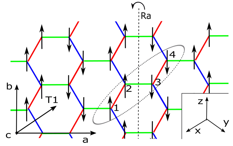
Figure 1: (Color online) Illustration of the zigzag order on the honeycomb lattice and associated symmetries. The dashed oval denotes the doubled magnetic unit cell.

III Topological magnons of the zigzag order in $\alpha$-RuCl₃

While the above framework and classification applies to a LSW theory of magnons in any magnetic order, to demonstrate its power, below we apply it to one specific example: the zigzag order in layered “Kitaev material” $\alpha$-RuCl₃. In $\alpha$-RuCl₃ the effective spin-$1/2$’s form a quasi-2d honeycomb network, where the dominant interactions between neighboring spins are written asRau et al. (2014); Janssen et al. (2016, 2017); Winter et al. (2017b); Wu et al. (2018)

$$H_{JK\Gamma h}=\sum_{\langle ij\rangle\in\alpha\beta(\gamma)}\big{[}KS^{\gamma}_{i}S^{\gamma}_{j}+\Gamma(S^{\alpha}_{i}S^{\beta}_{j}+S^{\beta}_{i}S^{\alpha}_{j})\big{]}$$

$$+J\sum_{\langle ij\rangle}\vec{S}_{i}\cdot\vec{S}_{j}-\sum_{i}\vec{h}\cdot\vec{S}_{i}.$$ (4)

where $J$, $K$ and $\Gamma$ denote the strength of nearest-neighbor (NN) Heisenberg, Kitaev and symmetric anisotropy terms. Without external fields, a “zigzag” magnetic order develops as illustrated in FIG. 1. Although the Bravais lattice translation $T_{1}$ is broken, its combination with time reversal i.e. magnetic translation $\tilde{T}_{1}=T_{1}\cdot{\mathcal{T}}$ is preserved by the zigzag order. Mirror reflection $R_{a}$ w.r.t. [100] plane is also preserved, where we have chosen the Bravais lattice vectors as $\hat{a}\parallel(-1,1,0),\leavevmode\nobreak\ \hat{b}\parallel(-1,-1,2),\leavevmode\nobreak\ \hat{c}\parallel(1,1,1)$.

Using parameters $K=-6.8$ meV, $\Gamma=9.5$ meV and $J\approx 0$ in model (4) from fitting recent neutron scattering dataRan et al. (2017), we plot the magnon band structure (for details see Supplemental Materials) of zigzag-ordered $\alpha$-RuCl₃ in FIG. 2. In the absence of external fields (FIG. 2(a)), there are three types of symmetry-protected magnon band crossings, protected by mirror $R_{a}$ (red), magnetic translation $\tilde{T}_{1}={\mathcal{T}}\cdot T_{1}$ (yellow) and magnetic mirror $\tilde{R}_{a}\equiv R_{a}\cdot\tilde{T}_{1}$ (green). A magnetic field along $\hat{a}$-axis breaks $\tilde{T}_{1}$ but preserves mirror $R_{a}$, leaving only the red-colored band crossings in FIG. 2(b). In contrast, an out-of-plane field along $\hat{c}$-axis breaks both $\tilde{T}_{1}$ and $R_{a}$ but preserves the magnetic mirror $\tilde{R}_{a}$, leaving only the green-colored band crossings in FIG. 2(c). Finally, a generic magnetic field along a low-symmetry direction will break all symmetries and lift all the magnon band touchings, as shown in FIG. 2(d).

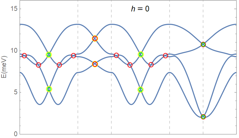
(a)

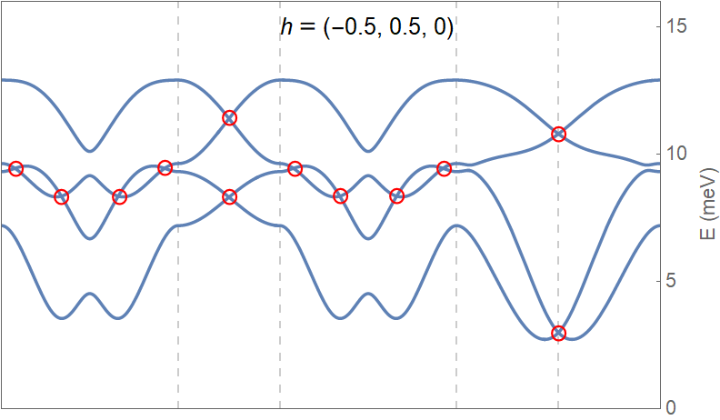
(b)

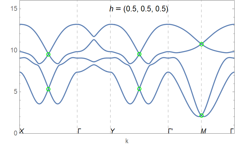
(c)

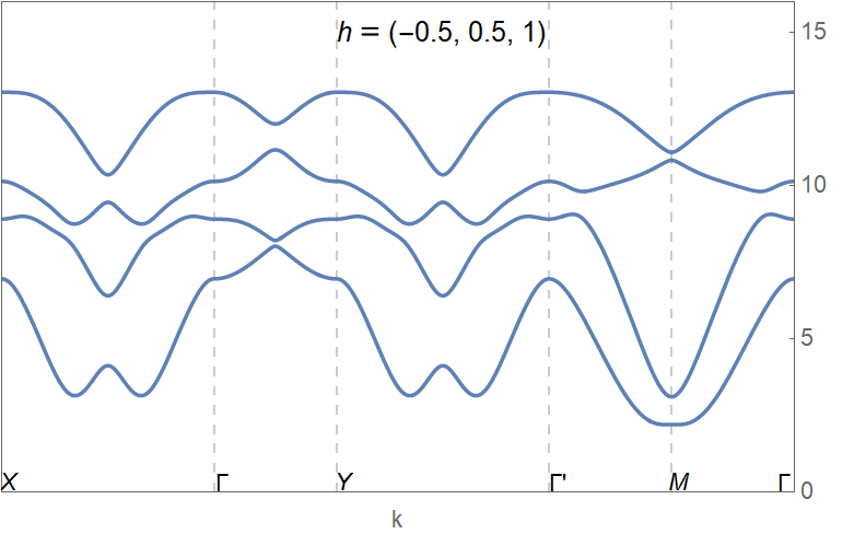
(d)

Figure 2: (Color online) Magnon band structures of zigzag-ordered $\alpha$-RuCl₃ under different magnetic fields, using parameters $K=-6.8$ meV, $\Gamma=9.5$ meV and $J\approx 0$ in model (4) fitted from neutron dataRan et al. (2017). Three types of magnon band crossings are protected by mirror $R_{a}$ (red circles), magnetic translation $\tilde{T}_{1}={\mathcal{T}}\cdot T_{1}$ (yellow circles) and magnetic mirror $\tilde{R}_{a}=R_{a}\cdot\tilde{T}_{1}$ (green circles).

After the magnetic field breaks all symmetries and lifts the band crossings, the topology of each magnon band is well-defined. In the absence of symmetries, each magnon band is characterized by an integer-valued Chern number $C\in{\mathbb{Z}}$ as shown in TABLE 2. Using the fermionization map (3) we can numerically computeFukui et al. (2005) the Chern number for each magnon band from the fermionized Hamiltonian ${\bf H}_{f}$. FIG. 3 shows how the Chern number $C$ for the lowest energy magnon band (see FIG. 2(d)) depends on NN Heisenberg interaction $J$ and magnetic field $\vec{h}$ in model (4). Due to the bulk-boundary correspondence, $C$ is also the number of chiral magnon edge states between the lowest energy band and the one above it. Choosing $J=0$ and out-of-plane field $h_{c}=2.7$ meV with Chern number $C=-1$ (see the arrow in FIG. 3(b)), we show the magnon spectrum on a cylinder geometry in FIG. 4, where each edge hosts a chiral magnon edge mode connecting the lowest magnon band and the one above it.

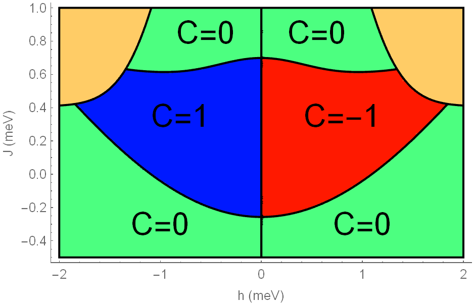
(a) In-plane field along $(\hat{a}+\hat{b})$ direction

(b) Out-of-plane field along (1,1,1)

Figure 3: (Color online) The Chern number $C$ of the lowest-energy magnon band (in FIG. 2(d)) of the zigzag order as a function of NN Heisenberg interaction $J$ and magnetic field $\vec{h}$ in model (4) with $K=-6.8$ meV, $\Gamma=9.5$ meVRan et al. (2017). The in-plane field aims at 45 degrees with both $\hat{a}$ and $\hat{b}$ axes. The zigzag order is unstable in the yellow regions.

In Ref.Winter et al., 2017b the importance of anharmonic interactions between magnons beyond LSW theory has been argued for the zero-field zigzag order in $\alpha$-RuCl₃. Since the interactions between magnons preserve the remaining symmetries of the magnetic order, the symmetry-protected topological magnons and surface states should be stable against certain amount of anharmonicity beyond LSW theory. While most results in the main text are obtained using parameters fitted from LABEL:Ran2017, in supplemental materials we also computed the magnon band topology for the model proposed in LABEL:Winter2017b for comparison, where magnon Chern bands are also induced by small magnetic fields along a range of directions.

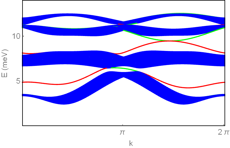
Figure 4: (Color online) Magnon spectrum on a cylinder with length $L_{a}=30$, periodic along $\hat{b}$ axis and open along $\hat{a}$ direction. Red and green denote topological edge states on the right and left edges respectively. We choose $J=0$ and $h_{c}=2.7$ meV in model (4), shown by the arrow in FIG. 3(b).

IV Summary

We develop a fermionization approach which maps any LSW theory to a short-ranged free-fermion Hamiltonian with exactly the same spectrum, while preserving all symmetries and band topology of the system. This allows us to classify and compute magnon band topology in various magnetic orders, hence providing a useful guide to the search for topological magnon bands and protected surface magnons in magnetic materials. Moreover this formulation can also be applied to classify and characterize the topology of various Bose-Einstein condensates.

As an application of this formulation, we investigate the zigzag magnetic order in layered honeycomb Kitaev material $\alpha$-RuCl₃. We identify symmetry-protected magnon band touchings at zero field, and magnon Chern bands under a small field along a wide range of directions. While recently the possibility of magnon Chern bands in $\alpha$-RuCl₃ has been proposed in the large field limitMcClarty et al. (2018), our studies reveal that a small field is enough to induce topological magnon bands. Our results provide a motivation for future neutron scattering and optical measurements to detect topological magnons in $\alpha$-RuCl₃ under a small magnetic field.

Supplemental Materials

Appendix A General setup of linear spin-wave theory

A.1 Equation-of-motion approach to spin waves

Consider a generic bilinear Hamiltonian of a spin system $\{{\bf S}_{i}=(S_{i}^{x},S_{i}^{y},S_{i}^{z})|i\in L\}$ on lattice $L$ ($\hbar$ is set to unity unless specifically mentioned):

$$H_{0}=\frac{1}{2}\sum_{i,j\in L}\sum_{\alpha,\beta}S_{i}^{\alpha}g_{i,j}^{\alpha,\beta}S_{j}^{\beta},$$ (5)

$$g_{i,j}^{\alpha,\beta}=g_{j,i}^{\beta,\alpha},\leavevmode\nobreak\ \leavevmode\nobreak\ |{\bf S}_{i}|=\bar{S}_{i}.$$

The spin magnitude $\bar{S}_{i}$ on different lattice sites $i\in L$ can in principle be different. In the classical (large spin) limit its ground state is magnetically ordered:

$$\langle{{\bf S}_{i}}\rangle=\bar{S}_{i}\hat{z}_{i}=(0,0,\bar{S}_{i}).$$ (6)

where $\hat{z}_{i}$ is the unit vector along the direction of ordered moment on site $i$. We’ve chosen a “local” coordinate frame $\{\hat{x}_{i},\hat{y}_{i}\perp\hat{x}_{i},\hat{z}_{i}=\hat{x}_{i}\times\hat{y}_{i}\}$ according to local ordering direction, so generically our couplings $g_{i,j}^{\alpha,\beta}$ in (5) are quite different from the usual couplings in a global Cartesian coordinate frame where $\hat{x}_{i}=\hat{x}_{j},\leavevmode\nobreak\ \forall\leavevmode\nobreak\ i,j$. For simplicity we choose all these local frames to be right-handed just like in the global frame. For example in our notation, an isotropic Heisenberg model with magnetic coupling $J_{i,j}$ is given by

$$g^{\alpha,\beta}_{i,j}=J_{i,j}\hat{\alpha}_{i}\cdot\hat{\beta}_{j},\leavevmode\nobreak\ \leavevmode\nobreak\ \leavevmode\nobreak\ \alpha,\beta=x,y,z.$$ (7)

Without loss of generality, a stable classical ground state (6) must minimize the classical energy (5), under the constraints

$${\bf S}_{i}\cdot{\bf S}_{i}=(\bar{S}_{i})^{2},\leavevmode\nobreak\ \leavevmode\nobreak\ \leavevmode\nobreak\ \forall\leavevmode\nobreak\ i\in L.$$ (8)

which can be enforced by introducing a Lagrangian multiplier per site $\{\lambda_{i}|i\in L\}$. In other words we need to solve the minimization problem of “constrained Hamiltonian” $F=H_{0}+$constraints. To be specific, a stable magnetic order (6) must satisfy the saddle-point condition

$$\frac{\partial F}{\partial S_{i}^{\alpha}}|_{{\bf S}_{i}=\langle{{\bf S}_{i}}\rangle}=\sum_{j,\beta}g_{i,j}^{\alpha,\beta}\langle{S_{j}^{\beta}}\rangle+2\lambda_{i}\langle{S_{i}^{\alpha}}\rangle=0,$$ (9)

$$F[{\bf S}_{i},\lambda_{i}]=\frac{1}{2}\sum_{i,j}\sum_{\alpha,\beta}S_{i}^{\alpha}g_{i,j}^{\alpha,\beta}S_{j}^{\beta}+\sum_{i}\lambda_{i}(|{\bf S}_{i}|^{2}-\bar{S}_{i}^{2}).$$

and the stability condition which guarantees positive stiffness for the order

$$\sum_{i,j}\sum_{\alpha,\beta}\delta S_{i}^{\alpha}\frac{\partial^{2}F}{\partial S_{i}^{\alpha}\partial S_{j}^{\beta}}|_{{\bf S}_{i}=\langle{{\bf S}_{i}}\rangle}\delta S_{j}^{\beta}=$$

$$\delta S_{i}^{\alpha}g_{i,j}^{\alpha,\beta}\delta S_{j}^{\beta}+2\sum_{i}\lambda_{i}\sum_{\alpha}(\delta S_{i}^{\alpha})^{2}\geq 0,\leavevmode\nobreak\ \leavevmode\nobreak\ \leavevmode\nobreak\ \forall\leavevmode\nobreak\ \{\delta{\bf S}_{i}\}.$$ (10)

The values of Lagrangian multipliers $\{\lambda_{i}\}$ are determined by requiring

$$\frac{\partial F}{\partial\lambda_{i}}|_{{\bf S}_{i}=\langle{{\bf S}_{i}}\rangle}=(\langle{{\bf S}_{i}}\rangle)^{2}-(\bar{S}_{i})^{2}=0.$$ (11)

The low-energy dynamics of the ordered magnets is captured by the spin waves, i.e. small deviations of spins from their ordered moments (6):

$${\bf s}_{i}\equiv{\bf S}_{i}-\langle{{\bf S}_{i}}\rangle\Rightarrow\langle{{\bf S}_{i}}\rangle\perp{\bf s}_{i}=(s_{i}^{x},s_{i}^{y},0),\leavevmode\nobreak\ \leavevmode\nobreak\ |{\bf s}_{i}|\ll\bar{S}_{i}.$$ (12)

Using the commutation relations for spin operators

$$[S_{i}^{\alpha},S_{j}^{\beta}]=\hskip 1.0pt\mathrm{i}\hskip 1.0pt\hbar\epsilon_{\alpha\beta\gamma}S_{i}^{\gamma}\leavevmode\nobreak\ \delta_{i,j}$$ (13)

we can obtain their linearized equations of motion (repeated Greek indices are summed over)

$$\frac{\text{d}s_{i}^{\alpha}}{\text{d}t}=\frac{[S_{i}^{\alpha},H_{0}]}{\hskip 1.0pt\mathrm{i}\hskip 1.0pt\hbar}=\sum_{j}\epsilon_{\alpha\mu\nu}S_{i}^{\nu}g^{\mu,\beta}_{i,j}S_{j}^{\beta}$$

$$=\sum_{j}\epsilon_{\alpha\mu\nu}g^{\mu,\beta}_{i,j}(\langle{S_{i}^{\nu}}\rangle s_{j}^{\beta}+s_{i}^{\nu}\langle{S_{j}^{\beta}}\rangle)$$

$$=\epsilon_{\alpha\mu\nu}\langle{S_{i}^{\nu}}\rangle(2\lambda_{i}s_{i}^{\mu}+\sum_{j}g^{\mu,\beta}_{i,j}s_{j}^{\beta})$$

$$=\bar{S}_{i}\epsilon_{\alpha\mu z}(2\lambda_{i}s_{i}^{\mu}+\sum_{j}g^{\mu,\beta}_{i,j}s_{j}^{\beta})=\sum_{j,\beta}M_{i\alpha,j\beta}s_{j}^{\beta},$$

$${\bf M}={\bf A}\cdot{\bf R},\leavevmode\nobreak\ \leavevmode\nobreak\ \leavevmode\nobreak\ A_{i\alpha,j\beta}=\epsilon_{\alpha\beta}\delta_{i,j}\bar{S}_{i}=(\hskip 1.0pt\mathrm{i}\hskip 1.0pt\sigma_{y})_{\alpha\beta}\delta_{i,j}\bar{S}_{i},$$

$$R_{i\alpha,j\beta}=2\lambda_{i}\delta_{i,j}\delta_{\alpha,\beta}+g_{i,j}^{\alpha,\beta}$$ (14)

where we have used (6) and saddle-point condition (9), and $\vec{\sigma}$ are Pauli matrices in the $(s^{x},s^{y})$ space. Clearly ${\bf A}$ is a $2N\times 2N$ ($N$ being the total number of spins) skew-symmetric real matrix, while ${\bf R}$ is a $2N\times 2N$ real symmetric matrix. According to stability condition (10), $R$ must be nonnegative definite i.e. its eigenvalues must be either zero or positive. By rescaling the spin wave variables to be ${\bf s}_{i}\rightarrow{\bf s}_{i}/\sqrt{\bar{S}_{i}}$ we can always rewrite the spin wave equations (14) into the standard form

$${\bf A}=\hskip 1.0pt\mathrm{i}\hskip 1.0pt\sigma_{y},$$

$${\bf R}_{{i\alpha,j\beta}}=\sqrt{\bar{S}_{i}}(g_{i,j}^{\alpha,\beta}+2\lambda_{i}\delta_{i,j}\delta_{\alpha,\beta})\sqrt{\bar{S}_{j}}.$$ (15)

where ${\bf R}$ remains a real symmetric nonnegative-definite matrix, describing short-ranged spin-spin interactions in the physical system. From now on we will refer ${\bf R}$ as the spin-wave (or magnon) Hamiltonian.

It is straightforward to show the above analysis applies even beyond quadratic magnetic Hamiltonian (5). For example in the presence of Zeeman field $\{h_{i}^{\alpha}\}$, the same analysis leads to the following real symmetric magnon Hamiltonian:

$${\bf R}_{{i\alpha,j\beta}}=\sqrt{\bar{S}_{i}}\big{[}g_{i,j}^{\alpha,\beta}+(2\lambda_{i}\delta_{\alpha,\beta}-h_{i}^{\alpha})\delta_{i,j}\big{]}\sqrt{\bar{S}_{j}}$$ (16)

which is stable only if ${\bf R}$ is non-negative definite.

As a result, quite generally, the following equation of motion (e.o.m.) determines the dynamics of spin waves

$$-\hskip 1.0pt\mathrm{i}\hskip 1.0pt\frac{\text{d}s_{i}^{\alpha}}{\text{d}t}=\sum_{j,\beta}\big{(}\sigma_{y}\cdot{\bf R}\big{)}_{i\alpha,j\beta}s_{j}^{\beta}$$ (17)

In this e.o.m. approach, eigenvalues of matrix $\sigma_{y}\cdot{\bf R}$ determine the magnon (or spin wave) spectrum. The fact that ${\bf R}={\bf R}^{\ast}$ is a real matrix implies a “particle-hole symmetry” of the eigenvalues of $\sigma_{y}{\bf R}$: a positive eigenvalue $\omega_{j}>0$ must appear in pair with a negative eigenvalue $-\omega_{j}<0$.

A.2 Holstein-Primakoff approach to spin waves

In Holstein-Primakoff formulationHolstein and Primakoff (1940), the spin wave dynamics is described in a boson representation of ordered spins in the semiclassical large-$S$ limit. Here we show that the Holstein-Primakoff approach to spin waves is in fact equivalent to the e.o.m. approach introduced earlier, and the two approaches are simply related by a unitary rotation $U$ in (20).

In the local frame (6) of ordered magnetic moments, the spin operators are written in terms of boson annihilation and creation operators $\{b_{i},b_{i}^{\dagger}\}$

$$S^{z}_{i}=\bar{S}_{i}-b_{i}^{\dagger}b_{i},$$

$$S^{+}_{i}\equiv S_{i}^{x}+\hskip 1.0pt\mathrm{i}\hskip 1.0ptS_{i}^{y}=\sqrt{2\bar{S}_{i}-b_{i}^{\dagger}b_{i}}\cdot b_{i}.$$ (18)

It’s straightforward to verify the spin commutation relation under the condition

$$b^{\dagger}_{i}b_{i}\leq 2\bar{S}_{i}.$$ (19)

A large-$S$ expansion in ${b_{i}^{\dagger}b_{i}}/{\bar{S}_{i}}\ll 1$ leads to

$$\begin{pmatrix}\hat{s}_{i}^{x}\\ \hat{s}_{i}^{y}\end{pmatrix}=\sqrt{{\bar{S}_{i}}}\cdot U\begin{pmatrix}b_{i}\\ b_{i}^{\dagger}\end{pmatrix}+O(b^{3}),$$

$$U=\frac{1}{\sqrt{2}}\begin{pmatrix}1&1\\ -\hskip 1.0pt\mathrm{i}\hskip 1.0pt&\hskip 1.0pt\mathrm{i}\hskip 1.0pt\end{pmatrix}=e^{\hskip 1.0pt\mathrm{i}\hskip 1.0pt\frac{\pi}{4}(1-\sigma_{z})}e^{\hskip 1.0pt\mathrm{i}\hskip 1.0pt\frac{\pi}{4}\sigma_{y}}.$$ (20)

Now we can perform large-$S$ expansion on Hamiltonian (5) and only keep terms up to quadratic order in $b,b^{\dagger}$. The result is the following linearized equation

$$\hat{H}_{eff}=\frac{1}{2}\sum_{i,j}\sum_{\alpha,\beta=x,y}\hat{s}_{i}^{\alpha}g_{i,j}^{\alpha,\beta}\hat{s}_{j}^{\beta}+2\sum_{i}\lambda_{i}b_{i}^{\dagger}b_{i}$$

$$=\frac{1}{2}\sum_{i,j}\sum_{\alpha,\beta}\hat{s}_{i}^{\alpha}R_{i\alpha,j\beta}\hat{s}_{j}^{\beta}+\text{const.}$$ (21)

where we have used the saddle-point condition (9) i.e.

$$\sum_{j}g_{i,j}^{\alpha,z}\langle{S_{j}^{z}}\rangle=-2\lambda_{i}\langle{S_{i}^{z}}\rangle\delta_{\alpha,z}$$ (22)

in our local coordinate frame. In terms of bosons the spin wave Hamiltonian (21) is written as

$$\hat{H}_{\text{H-P}}=\sum_{i,j}\phi^{\dagger}_{i}({\bf H}_{\bf b})_{i,j}\phi_{j},$$

$$\phi_{j}=(\phi_{j,1},\phi_{j,2})^{T}\equiv(b_{j},b_{j}^{\dagger})^{T},$$

$$({\bf H}_{\bf b})_{i,j}=U^{\dagger}\sqrt{\bar{S}_{i}}R_{i,j}\sqrt{\bar{S}_{j}}U=U^{\dagger}{\bf R}_{i,j}U$$ (23)

The fact that ${\bf R}$ is a real symmetric matrix imposes the following constraint on non-negative-definite Hamiltonian ${\bf H}$:

$$({\bf H}_{b})^{\ast}=\sigma_{x}{\bf H}_{b}\sigma_{x}$$ (24)

since $U^{\ast}=U\sigma_{x}=\sigma_{z}U$.

A.3 Structure of the magnon spectrum

Holstein-Primakoff Hamiltonian (23) is generally a Bogoliubov-de Gennes (BdG) Hamiltonian of boson operators $\{b_{i},b_{i}^{\dagger}\}$, involving both quadratic hopping and pairing terms of bosons. To diagonalize the boson BdG Hamiltonian ${\bf H}_{b}$ in (23), one needs to find a Bogoliubov transformation ${\bf W}_{b}\in SU(N,N)$ such that

$${\bf W}_{b}^{\dagger}{\bf H}_{b}{\bf W}_{b}={\bf\Lambda},\leavevmode\nobreak\ \leavevmode\nobreak\ \leavevmode\nobreak\ {\bf\Lambda}_{i\alpha,j\beta}=\lambda_{i\alpha}\delta_{i,j}\delta_{\alpha,\beta},$$

$${\bf W}_{b}^{\dagger}\sigma_{z}{\bf W}_{b}=\sigma_{z}.$$ (25)

where the 2nd condition ${\bf W}_{b}^{\dagger}\sigma_{z}{\bf W}_{b}=\sigma_{z}$ guarantees the boson commutation relation

$$[b_{i},b^{\dagger}_{j}]=\delta_{i,j}\Leftrightarrow[\phi_{i\alpha},\phi_{j\beta}^{\dagger}]=(\sigma_{z})_{\alpha,\beta}\delta_{i,j}.$$ (26)

remains invariant under the Bogoliubov transformation ${\bf W}_{b}$. It’s straightforward to show that we are effectively digonalizing matrix $\sigma_{z}{\bf H}_{b}$ since

$$\sigma_{z}{\bf H}_{b}\cdot{\bf W}_{b}={\bf W}_{b}\cdot\sigma_{z}{\bf\Lambda}$$ (27)

Condition (24) guarantees that eigenstates with opposite frequency $\pm E$ always show up in pairs:

$$\sigma_{z}{\bf H}_{b}\cdot\vec{v}_{E}=E\leavevmode\nobreak\ \vec{v}_{E}\Longleftrightarrow\sigma_{z}{\bf H}_{b}\cdot\sigma_{x}\vec{v}_{E}^{\ast}=-E\leavevmode\nobreak\ \sigma_{x}\vec{v}_{E}^{\ast}.$$

in other words

$${\bf W}_{b}=({\bf V},\sigma_{x}{\bf V}^{\ast})=\sigma_{x}{\bf W}_{b}^{\ast}\sigma_{x}.$$ (28)

where ${\bf V}$ is a $2N\times N$ matrix satisfying normalization condition

$${\bf V}^{\dagger}\sigma_{z}{\bf V}=\hat{1}_{N\times N}.$$ (29)

$N$ being the total number of spins. This means each eigenvalue in ${\bf\Lambda}$ is at least two-fold degenerate i.e.

$${\bf\Lambda}=\sigma_{0}\otimes{\bf\Omega},\leavevmode\nobreak\ \leavevmode\nobreak\ \leavevmode\nobreak\ \Omega_{i,j}=\delta_{i,j}\omega_{i}\geq 0.$$ (30)

Therefore condition (24), equivalent to condition ${\bf R}={\bf R}^{\ast}$ in can be viewed as a “particle-hole symmetry” which relates positive-eigenvalue ($+\omega_{i}$) states to negative-eigenvalue ($-\omega_{i}$) ones.

Clearly matrix $\sigma_{z}{\bf H}_{b}$ has the same magnon spectrum as the equation of motion (e.o.m.) approach (17) to spin waves, since

$$\sigma_{z}{\bf H}_{b}=\sigma_{z}U^{\dagger}{\bf R}U$$

$$=U^{-1}\big{(}U\sigma_{z}U^{\dagger}{\bf R}\big{)}U=U^{-1}(\sigma_{y}{\bf R})U$$ (31)

The corresponding basis transformation ${\bf B}$ that diagonalizes spin wave equation of motion (17) is

$${\bf B}=U{\bf W}U^{\dagger}\Longrightarrow\sigma_{y}{\bf R}\cdot{\bf B}={\bf B}\cdot(\sigma_{y}\otimes{\bf\Omega})$$ (32)

It’s straightforward to check the following properties for ${\bf B}$ from (25) and (24):

$${\bf B}^{\dagger}\sigma_{y}{\bf B}=\sigma_{y},\leavevmode\nobreak\ \leavevmode\nobreak\ \leavevmode\nobreak\ {\bf B}^{\ast}={\bf B}.$$ (33)

Therefore ${\bf B}$ is a real symplectic matrix, which diagonalizes the non-negative-definite matrix ${\bf R}$ in (17) by:

$${\bf B}^{\dagger}{\bf R}{\bf B}={\bf\Lambda}=\sigma_{0}\otimes{\bf\Omega},\leavevmode\nobreak\ \leavevmode\nobreak\ \leavevmode\nobreak\ {\bf B}\in Sp(2N,\mathbb{R}),$$ (34)

$$\Leftrightarrow\sigma_{y}{\bf R}={\bf B}(\sigma_{y}\otimes{\bf\Omega}){\bf B}^{-1}={\bf B}{\bf\Omega}{\bf B}^{\dagger}\sigma_{y}.$$

The equivalence between e.o.m. approach and Holstein-Primakoff approach to spin waves is summarized in TABLE 1.

Appendix B Implementing symmetries in spin waves

The many-spin Hamiltonian (5) can preserve various symmetries, such as global $SO(3)$ spin rotations, time reversal ${\mathcal{T}}$ and space group symmetries. We call this symmetry group $G_{0}$. Formation of magnetic orders generally breaks the original symmetry $G_{0}$ down to a subgroup $G_{s}\subset G_{0}$, which does not include global time reversal symmetry ${\mathcal{T}}$. However the combination of time reversal and another operation may still be a symmetry even in the presence of the magnetic order: e.g. a collinear ferromagnetic order preserves the combination of time reversal ${\mathcal{T}}$, and a spin rotation $e^{\hskip 1.0pt\mathrm{i}\hskip 1.0pt\pi\sum_{j}\hat{S}_{j}^{x}}$ by angle $\pi$ along an axis perpendicular to the ordering direction. An antiferromagnetic Neel order on a bipartite lattice typically preserves the combination of ${\mathcal{T}}$, and some space group operation exchanging two sublattices, such as translation on a square lattice.

In the following we discuss how these unbroken symmetries act on a spin-wave system (17) or (23). A generic symmetry $g$ is implemented on a magnon Hamiltonian ${\bf R}$ in the following way:

$${\bf R}\overset{g}{\longrightarrow}O_{g}{\bf R}O_{g}^{\dagger},\leavevmode\nobreak\ \leavevmode\nobreak\ \leavevmode\nobreak\ O_{g}\in SO(2N),\leavevmode\nobreak\ \leavevmode\nobreak\ \leavevmode\nobreak\ \forall\leavevmode\nobreak\ g\in G_{s}.$$ (35)

A symmetry element $g\in G_{s}$ can be either unitary such as spin rotations and crystalline symmetries, or anti-unitary such as time reversal or its combination with a unitary operation. They have quite different effects on the spin waves. In particular while a unitary symmetry preserves the handedness of the local coordinate frame for the ordering moments, an anti-unitary symmetry switches the handedness, since time reversal operation ${\mathcal{T}}$ will reverse all spin components ${\bf S}_{i}\overset{{\mathcal{T}}}{\longrightarrow}-{\bf S}_{i}$. In terms of their matrix representation $O_{g}$ in (35), they differ in the following way:

$$[O_{g},\sigma_{y}]=0,\leavevmode\nobreak\ \leavevmode\nobreak\ \leavevmode\nobreak\ \forall\leavevmode\nobreak\ g\leavevmode\nobreak\ \text{is unitary}\Leftrightarrow O_{g}\in SO(2N)\cap Sp(2N,\mathbb{R})\simeq U(N).$$ (36)

and

$$\{O_{g},\sigma_{y}\}=0,\leavevmode\nobreak\ \leavevmode\nobreak\ \leavevmode\nobreak\ \forall\leavevmode\nobreak\ g\leavevmode\nobreak\ \text{is anti-unitary}.$$ (37)

It’s straightforward to see that the spin-wave e.o.m. (17) remains invariant under either a unitary or anti-unitary symmetry $g$, since time reverses $t\overset{{\mathcal{T}}}{\rightarrow}-t$ under an anti-unitary symmetry $g$.

As show in TABLE 1, the symmetry operations $\{O_{g}|g\in G_{s}\}$ on a “magnon Hamiltonian” ${\bf R}$ can also be translated into the associated Holstein-Primakoff formalism, and the corresponding free fermion system. In particular, each unitary symmetry $g$ in a magnon system is mapped to a unitary symmetry in the fermion system; while each anti-unitary symmetry $h$ in a magnon system is mapped to an anti-unitary one in free fermions.

More specifically let’s consider $h=\mathcal{K}$ (complex conjugation) and we have

$${\mathcal{T}}\hskip 1.0pt\mathrm{i}\hskip 1.0pt{\mathcal{T}}^{-1}=-\hskip 1.0pt\mathrm{i}\hskip 1.0pt,\leavevmode\nobreak\ \leavevmode\nobreak\ {\mathcal{T}}\sigma_{y}{\mathcal{T}}=-\sigma_{y},$$

$${\mathcal{T}}{\bf R}{\mathcal{T}}^{-1}={\bf R},\leavevmode\nobreak\ \leavevmode\nobreak\ {\mathcal{T}}{\bf B}{\mathcal{T}}^{-1}={\bf B},$$ (38)

$${\mathcal{T}}U{\mathcal{T}}^{-1}=U^{\ast}=U\sigma_{x},\leavevmode\nobreak\ \leavevmode\nobreak\ {\mathcal{T}}{\bf H}{\mathcal{T}}^{-1}={\bf H}^{\ast}=\sigma_{x}{\bf H}\sigma_{x}.$$

Therefore in coplanar (and collinear) magnetic orders whose magnetic moments are all perpendicular to e.g. $\hat{x}$-axis, the combined $\pi$-spin-rotation and time reversal symmetry is implemented by

$$e^{\hskip 1.0pt\mathrm{i}\hskip 1.0pt\pi\sum_{j}\hat{S}^{x}_{j}}{\mathcal{T}}=\sigma_{z}\cdot\mathcal{K}$$ (39)

As a result, spin wave Hamiltonians (21) and (23) for coplanar magnetic orders satisfy

$$\sigma_{z}{\bf R}\sigma_{z}={\bf R}\Leftrightarrow\sigma_{x}{\bf H}\sigma_{x}={\bf H},$$

$$\Longrightarrow\sigma_{z}{\bf B}\sigma_{z}={\bf B}.$$ (40)

since $U^{\dagger}\sigma_{z}U=-\sigma_{x}$.

Spin rotational symmetries also exist in certain magnets, e.g. collinear magnetic orders preserve a $U(1)$ spin rotation along the magnetization direction ($\hat{z}$ axis). A global spin rotation by angle $\phi$ along $\hat{z}$-axis is implemented by

$$\hat{U}_{z}(\phi)\equiv e^{\hskip 1.0pt\mathrm{i}\hskip 1.0pt\phi\sum_{j}\hat{S}_{j}^{z}}=e^{\hskip 1.0pt\mathrm{i}\hskip 1.0pt\frac{\phi}{2}\sigma_{y}}$$ (41)

Therefore in collinear magnetic orders, $U(1)_{{\bf S}^{z}}$ spin rotational symmetry indicates

$$\sigma_{y}{\bf R}\sigma_{y}={\bf R}\Leftrightarrow\sigma_{z}{\bf H}\sigma_{z}={\bf H},$$

$$\Longrightarrow\sigma_{y}{\bf B}\sigma_{y}={\bf B}.$$ (42)

Appendix C Relation to previous formulationShindou et al. (2013a)

Previously in LABEL:Shindou2013, the Chern number of a magnon band has been computed using the projection operator into one magnon band. In particular, LABEL:Shindou2013 adopted a Cholesky decompostionColpa (1978) of the Holstein-Primakoff ${\bf H}_{b}$ to obtain the eigenstate wavefunctions of the LSW theory. Below we discuss the difference between our fermionization map (3) in TABLE 1 and the formulation adopted in LABEL:Shindou2013.

In LABEL:Shindou2013, a Cholesky decomposition for Hermitian positive definite matrix ${\bf H}_{b}=U{\bf R}U^{\dagger}$ is performed

$${\bf H}_{b}={\bf K}^{\dagger}\cdot{\bf K}$$ (43)

and leads to a free-fermion Hamiltonian

$$\tilde{\bf H}_{f}={\bf K}\cdot\sigma_{z}\cdot{\bf K}^{\dagger}$$ (44)

which can be diagonalized by a unitary matrix

$$\tilde{\bf W}_{f}={\bf K}{\bf W}_{b}{\bf\Omega}^{-1/2}$$ (45)

Compared to the unitary matrix ${\bf W}_{f}$ which diagonalizes the fermionized Hamiltonian ${\bf H}_{f}$ in TABLE 1, this unitary transformation differs by a unitary transformation ${\bf U}_{f}$:

$${\bf W}_{f}=U\sqrt{{\bf H}_{b}}{\bf W}_{b}{\bf\Omega}^{-1/2}={\bf U}_{f}\tilde{\bf W}_{f},\leavevmode\nobreak\ \leavevmode\nobreak\ \leavevmode\nobreak\ {\bf U}_{f}\equiv U\sqrt{{\bf H}_{b}}\cdot{\bf K}^{-1},\leavevmode\nobreak\ \leavevmode\nobreak\ \leavevmode\nobreak\ U=e^{\hskip 1.0pt\mathrm{i}\hskip 1.0pt\frac{\pi}{4}(1-\sigma_{z})}e^{\hskip 1.0pt\mathrm{i}\hskip 1.0pt\frac{\pi}{4}\sigma_{y}}.$$ (46)

It’s straightforward to show that ${\bf U}_{f}$ is unitary

$${\bf U}_{f}^{\dagger}{\bf U}_{f}=\big{(}{\bf K}^{\dagger}\big{)}^{-1}{\bf H}_{b}{\bf K}^{-1}=1.$$ (47)

Though only differing by a unitary transformation, there is one major advantage of our fermionized Hamiltonian ${\bf H}_{f}$ over $\tilde{\bf H}_{f}$ previously used in LABEL:Shindou2013. In our fermionization map, the LSW Hamiltonian matrix ${\bf R}$ and its free-fermion counterpart ${\bf H}_{f}$ share the same symmetry implementation $O_{g}$ for symmetry element $g$, where $O_{g}$ is independent of the Hamiltonian as long the symmetry is preserved. In contrast, for the free-fermion Hamiltonian $\tilde{\bf H}_{f}$ introduced in LABEL:Shindou2013, the corresponding symmetry operation

$$\tilde{O}_{g}={\bf U}_{f}^{\dagger}O_{g}{\bf U}_{f},\leavevmode\nobreak\ \leavevmode\nobreak\ \leavevmode\nobreak\ [\tilde{O}_{g},\tilde{\bf H}_{f}]=0.$$ (48)

depends on the specific Hamiltonian ${\bf H}_{b}$ (or ${\bf R}$). In particular for the periodic band structure of a LSW, calculations are performed in momentum (${\bf k}$) space after the Fourier transform. Since the Holstein-Primakoff Hamiltonian ${\bf H}_{b}({\bf k})$ depends on momentum ${\bf k}$, the associated symmetry operator $\tilde{O}_{g}({\bf k})$ will also change with ${\bf k}$ and may not even be a smooth function of ${\bf k}$.

Appendix D Topological triviality of magnon ground states and Goldstone modes

Previously we have established a mapping from a non-interacting magnon system to a free fermion system. While this map allows us to understand the band topology of magnons by examining its free-fermion counterparts, it is not a surjective map. In other words, not all free-fermion states have their counterparts in the magnon system. In this section, we establish a most significant difference between magnon and free-fermion systems. In gapped topological insulators and superconductors of fermions, the ground state can have a nontrivial topology, and host in-gap surface states between the empty conduction bands (positive) and filled valence bands (negative energy). In sharp contrast in a generic gapped magnon system, the magnetic ground state must have a trivial topology, and hence there can be no symmetry-protected in-gap surface states in any gapped magnon system. In this section, we always refer to the gap around zero energy unless further specified.

First of all, the “wavefunction” matrix ${\bf B}$ of spin wave Hamiltonian ${\bf R}$ has the following properties

$${\bf B}^{\dagger}\sigma_{y}{\bf B}=\sigma_{y},\leavevmode\nobreak\ \leavevmode\nobreak\ \leavevmode\nobreak\ {\bf B}^{\ast}={\bf B}$$ (49)

and hence belongs to the symplectic group ${\bf B}\in Sp(2N,\mathbb{R})$. As a general property of a real symplectic matrix, we have

$${\bf B}=O{\bf Z}O^{\prime},\leavevmode\nobreak\ \leavevmode\nobreak\ \leavevmode\nobreak\ {\bf Z}=\begin{pmatrix}D&\\ &D^{-1}\end{pmatrix},$$ (50)

$$O,O^{\prime}\in Sp(2N,\mathbb{R})\cap SO(2N)\cong U(N).$$

where $D$ is a positive-definite and diagonal $N\times N$ matrix. As shown in TABLE 1 the spin wave “Hamiltonian” ${\bf R}$, a real symmetric non-negative-definite matrix, can be written as

$${\bf R}=\sigma_{y}{\bf B}\mathbf{\Omega}{\bf B}^{\dagger}\sigma_{y}.$$ (51)

where $\mathbf{\Omega}$ is a non-negative-definite diagonal matrix of magnon frequencies.

Now let’s assume a gapped magnon spectrum (without massless Goldstone modes) with a finite gap $2\Delta>0$ i.e.

$$\mathbf{\Omega}_{i,j}=\delta_{i,j}\omega_{i}\geq 0,\leavevmode\nobreak\ \leavevmode\nobreak\ \leavevmode\nobreak\ \omega_{i}\geq\Delta>0.$$ (52)

In order to study the in-gap surface states of a magnon system without loss of generality, we follow the spectrum flattening trick used in free-fermion systems. More specifically, all magnon frequencies $\{\omega_{i}\geq\Delta>0\}$ in the gapped spectrum are adiabatically tuned to the same positive frequency

$$\omega_{i}\equiv\Delta>0,\leavevmode\nobreak\ \forall\leavevmode\nobreak\ i\Longleftrightarrow\mathbf{\Omega}=\Delta\cdot\hat{1}_{N\times N}.$$ (53)

in the “flat band” limit. Any zero-energy topological surface states below the gap should not be affected in this spectral flattening process.

With the flattened spectrum (53), due to property (50) of symplectic matrix ${\bf B}$, the spin wave Hamiltonian (51) can be written as

$${\bf R}=\Delta\cdot\sigma_{y}O{\bf Z}^{2}O^{\dagger}\sigma_{y}=\Delta\cdot O{\bf Z}^{-2}O^{\dagger}=\Delta\cdot e^{{\bf M}_{R}},$$ (54)

$${\bf M}_{R}\equiv\sigma_{y}O\log({\bf Z}^{2})O^{\dagger}\sigma_{y}=-2O\big{(}\sigma_{z}\otimes\log D\big{)}O^{\dagger}.$$

The existence of an exponential map from invertible real symmetric matrix ${\bf M}_{R}$ to spin wave Hamiltonian ${\bf R}$ is crucial to establish the trivial topology of a magnetic ground state. It provides a continuous family of gapped magnon Hamiltonians

$${\bf R}(\lambda)=\Delta\cdot e^{\lambda{\bf M}_{R}}=\Delta\cdot\sigma_{y}{\bf B}(\lambda){\bf B}^{\dagger}(\lambda)\sigma_{y},\leavevmode\nobreak\ \leavevmode\nobreak\ 0\leq\lambda\leq 1.$$ (55)

with wavefunction matrix

$${\bf B}(\lambda)=O{\bf Z}^{\lambda}O^{\prime}\in Sp(2N,\mathbb{R})$$ (56)

Clearly the whole family of spin wave Hamiltonians all shares the flat-band spectrum (53). It adiabatically connects an arbitrary gapped magnon Hamiltonian ${\bf R}={\bf R}(\lambda=1)$ to a “trivial” Hamiltonian that is proportional to the identity matrix

$${\bf R}(\lambda=0)=\Delta\cdot\hat{1},$$ (57)

$${\bf B}(\lambda=0)=OO^{\prime}\in Sp(2N,\mathbb{R})\cap SO(2N)\cong U(N).$$

In general the magnon system can preserve certain global and/or crystalline symmetries belonging to a symmetry group $G_{s}$. As discussed earlier, any symmetry element $g\in G_{s}$ is implemented on the magnon Hamiltonian ${\bf R}$ by an orthogonal rotation $O_{g}$

$${\bf R}=O_{g}{\bf R}O_{g}^{\dagger},\leavevmode\nobreak\ \leavevmode\nobreak\ \leavevmode\nobreak\ O_{g}\in SO(2N).$$ (58)

The exponential map (54) of spin-wave Hamiltonian ${\bf R}$ therefore implies that

$$[{\bf M}_{R},O_{g}]=0$$ (59)

As a result, the whole family of gapped Hamiltonian preserves the same symmetry $g$ since

$${\bf R}(\lambda)=O_{g}{\bf R}(\lambda)O_{g}^{\dagger},\leavevmode\nobreak\ \leavevmode\nobreak\ \leavevmode\nobreak\ 0\leq\lambda\leq 1.$$ (60)

Hence all symmetry operations of group $G_{s}$, which are responsible for the protected surface states, are all preserved when magnon system ${\bf R}$ is adiabatically tuned into the trivial magnon system (57) without closing the gap.

From Table 1 it’s straightforward to show this trivial spin-wave Hamiltonian ${\bf R}(\lambda=0)$ in (57) is mapped to a topologically-trivial free-fermion Hamiltonian

$${\bf H}_{f}(\lambda=0)=\Delta\cdot\sigma_{y}$$ (61)

which obviously has trivial band topology and no zero-energy in-gap surface states.

Therefore by establishing a gapped family of spin-wave Hamiltonians that connects an arbitrary gapped magnon system to the trivial magnon flat bands, we proved that no symmetry-protected topological surface states exist below the finite bulk gap in a generic gapped magnon system.

One natural question follows: what about gapless magnon systems with massless Goldstone modes near zero energy in their spectra? Can they support topological surface states near zero energy? The answer is again negative. This can be understood as follows. The topology of various band touchings, such as point nodes, line nodes and fermi surfaces had been classified in free fermion systemsHorava (2005); Wang and Lee (2012); Matsuura et al. (2013); Zhao and Wang (2013) by a dimensional reduction approach. In particular the classification of stable fermi surface of codimension $d_{c}$ coincides with the classification of gapped free-fermion ground states (hosting zero-energy surface states) in spatial dimension $d=d_{c}-1$. The idea is to consider a gapped and closed submanifold of the Brillouin zone that encloses the nodal points/lines or fermi surfaces, which has dimension $d=d_{c}-1$. Here we can adopt exactly the same strategy in a magnon system. However as shown above, all magnon ground states must be topologically trivial, without any robust zero-energy surface states of magnon systems in any spatial dimension. As a result, the topology of massless Goldstone modes near zero energy in a magnon system must also be trivial, without any protected surface states below the bulk gap around zero energy.

Appendix E Classifying space and topology for each magnon band

Previously we have shown that all negative-frequency magnon bands as a whole must be topologically trivial. This however does not imply that each magnon band itself must also be topologically trivial. In this section, based on the mapping from spin waves to free fermions in Table 1, we further show that a finite energy magnon band with arbitrary (unitary or anti-unitary) symmetries can have the same topology as a free-fermion energy band (Altland-Zirnbauer class AAltland and Zirnbauer (1997)) with proper unitary symmetries. This allows us to classify the possible topological bands and topological band touchings of spin waves, with various symmetries and in all spatial dimensions.

A spin wave spectrum $\sigma_{z}\otimes\mathbf{\Omega}$ always has the particle-hole symmetry relating positive and negative energy eigenstates. As proven earlier, all negative-energy bands as a whole have a trivial topology, Therefore we will focus on the magnon bands at positive energy $\{\omega_{j}\geq 0\}$. Following Kitaev’s K-theory approach to classify free-fermion systemsKitaev (2009); Wen (2012); Morimoto and Furusaki (2013), without loss of generality, we again consider the following flat-band spectrum with two flat bands $\epsilon_{1}>\epsilon_{2}>0$:

$$\mathbf{\Omega}=\begin{pmatrix}\epsilon_{1}&&&&&\\ &\cdots&&&&\\ &&\epsilon_{1}&&&\\ &&&\epsilon_{2}&&\\ &&&&\cdots&\\ &&&&&\epsilon_{2}\end{pmatrix}$$

$$=\big{[}\epsilon_{1}\cdot\hat{1}_{M\times M}\big{]}\oplus\big{[}\epsilon_{2}\cdot\hat{1}_{(N-M)\times(N-M)}\big{]}$$

$$=\Delta\cdot\hat{1}_{N\times N}+\epsilon\cdot\hat{\mathcal{D}}_{N\times N}.$$ (62)

where we defined

$$\hat{\mathcal{D}}_{N\times N}\equiv\big{[}+\hat{1}_{M\times M}\big{]}\oplus\big{[}-\hat{1}_{(N-M)\times(N-M)}\big{]},$$ (63)

$$\Delta\equiv\frac{\epsilon_{1}+\epsilon_{2}}{2}>\epsilon\equiv\frac{\epsilon_{1}-\epsilon_{2}}{2}>0.$$ (64)

Although the two bands at $\epsilon_{1,2}$ as a whole are topologically trivial, each band itself can have a nontrivial topology. This can be understood as follows. We can use the same symmetric continuous path (56) to deform the eigenstate wavefunctions of linear spin waves, while keeping the spectrum the same. This leads to the following family of symmetric linear spin wave Hamiltonian matrix

$${\bf R}(\lambda)=\sigma_{y}{\bf B}(\lambda){\bf\Omega}{\bf B}^{\dagger}(\lambda)\sigma_{y}$$ (65)

which interpolates the original spin wave Hamiltonian ${\bf R}={\bf R}(\lambda=1)$ and the following simplified Hamiltonian

$${\bf R}(\lambda=0)={\bf B}_{0}{\bf\Omega}{\bf B}_{0}^{\dagger},\leavevmode\nobreak\ \leavevmode\nobreak\ \leavevmode\nobreak\ {\bf B}_{0}^{\dagger}={\bf B}(\lambda=0)=OO^{\prime}\in U(N)$$ (66)

Due to the two-flat-band structure of spectrum (62), when no other symmetries are considered, the classifying space of linear spin wave Hamiltonian (66) is given by the following Grassmannian:

$$\frac{U(N)}{U(M)\times U(N-M)}$$ (67)

This leads to a classifying space $\mathcal{C}_{d}$ without other symmetries ($d$ is the spatial dimension), belonging to symmetry class A in the Altland-Zirnbauer 10-fold wayAltland and Zirnbauer (1997). This exactly match the classification of the topology of each band in the corresponding free fermion Hamiltonian, ${\bf H}_{f}=\sqrt{\bf R}\sigma_{y}\sqrt{\bf R}$ obtained from linear spin wave Hamiltonian ${\bf R}$ via the fermionization map. This demonstrates that one specific band of the free fermion Hamiltonians obtained by fermionizing the linear spin wave can realize all possible band topology within the corresponding fermion symmetry class. Therefore, we can fully classify the band topology of linear spin waves by looking into their free fermion partners obtained via the fermionization map.

Appendix F Linear spin wave theory for the zigzag order in $\alpha$-RuCl₃

Below we describe how to use LSW theory to compute the magnon band structure for the zigzag orderLittle et al. (2017); Wang et al. (2017); Cookmeyer and Moore (2018) in the following model for $\alpha$-RuCl₃:

$$H_{JK\Gamma h}=\sum_{\langle ij\rangle\in\alpha\beta(\gamma)}\big{[}KS^{\gamma}_{i}S^{\gamma}_{j}+\Gamma(S^{\alpha}_{i}S^{\beta}_{j}+S^{\beta}_{i}S^{\alpha}_{j})\big{]}+J\sum_{\langle ij\rangle}\vec{S}_{i}\cdot\vec{S}_{j}+\sum_{i}\vec{h}\cdot\vec{S}_{i}.$$ (68)

In the first step, we find the classical spin configuration that minimizes the free energy. Luttinger-Tisza methodLuttinger and Tisza (1946) is widely adopted, which applies to the zero magnetic field case or a small magnetic field along specific directions. Here, we start from the zigzag magnetic order and consider four spins within one doubled magnetic unit cell. We can numerically optimize energy in eight-dimensional space of variables $\{(\theta_{i},\phi_{i})\}$, where $\theta_{i},\phi_{i}$ are the polar and azimuthal angles for the spin orientation. Considering small deviations $\mathbb{X}_{\mathbb{k}}=(S_{1,\mathbb{k}}^{x},S_{1,\mathbb{k}}^{y},S_{2,\mathbb{k}}^{x},S_{2,\mathbb{k}}^{y},S_{3,\mathbb{k}}^{x},S_{3,\mathbb{k}}^{y},S_{4,\mathbb{k}}^{x},S_{4,\mathbb{k}}^{y})$ from the ordered (lowest-energy) magnetic moment, we expand the free energy around its minimum and obtain the following LSW energy functional

$$H_{2}=\sum_{\mathbb{k}}\mathbb{X}_{\mathbb{k}}^{\dagger}\cdot\mathcal{H}_{\mathbb{k}}\cdot\mathbb{X}_{\mathbb{k}}$$ (69)

where $\mathcal{H}_{\mathbb{k}}$ is given by

$$\mathcal{H}_{\mathbb{k}}=\left(\begin{array}[]{c c c c c c c c}A&0&B&C&0&0&E_{1}&F_{1}\\ 0&A&C&D&0&0&F^{\prime}_{1}&G_{1}\\ B^{\dagger}&C^{\dagger}&A&0&E&F&0&0\\ C^{\dagger}&D^{\dagger}&0&A&F^{\prime}&G&0&0\\ 0&0&E^{\dagger}&F^{\prime\dagger}&A_{1}&0&B_{1}&C_{1}\\ 0&0&F^{\dagger}&G^{\dagger}&0&A_{1}&C_{1}&D_{1}\\ E_{1}^{\dagger}&F_{1}^{\prime\dagger}&0&0&B_{1}^{\dagger}&C_{1}^{\dagger}&A_{1}&0\\ F_{1}^{\dagger}&G_{1}^{\dagger}&0&0&C_{1}^{\dagger}&D_{1}^{\dagger}&0&A_{1}\end{array}\right)$$ (78)

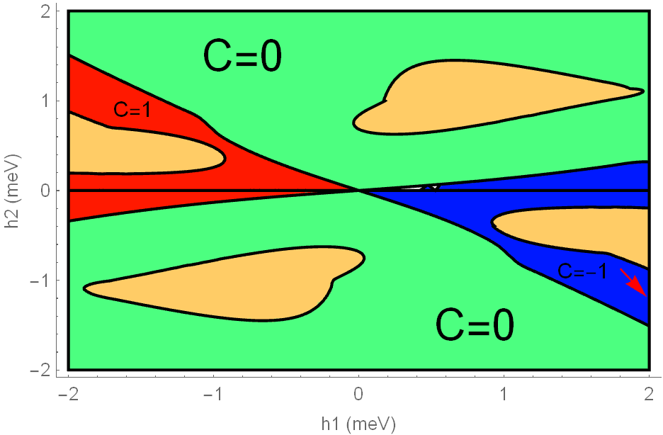
(a) Field within [110] plane.

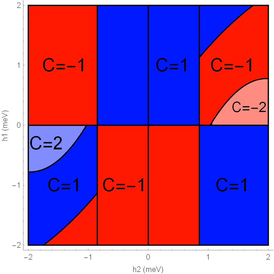
(b) Field within [010] plane.

Figure 5: (Color online) The Chern number $C$ of the lowest-energy magnon band of the zigzag order in model (68), with parameters $K=-5$meV, $\Gamma=2.5$meV, $J_{1}=-0.5$meV and $J_{3}=0.5$meV from LABEL:Winter2017b. $h_{1}$ denotes the in-plane component and $h_{2}$ is the out-of-plane component of the magnetic field. The zigzag order is unstable in the yellow regions.

For all calculations performed in this work, we numerically found that sublattices 1 and 2 share the same ordered moment ${\bf n}$, while sublattices 3 and 4 share the opposite moment $-{\bf n}$. We represent them as $(\theta_{1},\phi_{1})$ and $(\theta_{3},\phi_{3})$. The elements of $\mathcal{H}_{\mathbb{k}}$ are written as below

$$A= -2J-K\sin^{2}\theta_{1}+(J+K)\cos\theta_{1}\cos\theta_{3}-\Gamma\sin 2\theta_{1}(\cos\phi_{1}+\cos\phi_{3})+\sin\theta_{1}\sin\theta_{3}(J\cos(\phi_{1}-\phi_{3})$$ (79)

$$+\Gamma\sin(\phi_{1}+\phi_{3}))-2\vec{h}\cdot\hat{v}(\theta_{1},\phi_{1}),$$

$$A_{1}= -2J-K\sin^{2}\theta_{3}+(J+K)\cos\theta_{1}\cos\theta_{3}-\Gamma\sin 2\theta_{3}(\cos\phi_{1}+\cos\phi_{3})+\sin\theta_{1}\sin\theta_{3}(J\cos(\phi_{1}-\phi_{3})$$

$$+\Gamma\sin(\phi_{1}+\phi_{3}))+2\vec{h}\cdot\hat{v}(\theta_{3},\phi_{3}),$$

$$B= J(1+e^{-ik_{b}})+K(\cos^{2}\theta_{1}+e^{-ik_{b}}\sin^{2}\theta_{1}),$$

$$B_{1}= J(1+e^{-ik_{b}})+K(\cos^{2}\theta_{3}+e^{-ik_{b}}\sin^{2}\theta_{3}),$$

$$C= (-K\cos\theta_{1}\cos\phi_{1}-J\sin\theta_{1})\sin\phi_{1}+e^{-ik_{b}}\cos\phi_{1}(J\sin\theta_{1}+K\cos\theta_{1}\sin\phi_{1}),$$

$$C_{1}= (K\cos\theta_{3}\cos\phi_{3}+J\sin\theta_{3})\sin\phi_{3}-e^{-ik_{b}}\cos\phi_{3}(J\sin\theta_{3}+K\cos\theta_{3}\sin\phi_{3}),$$

$$D= (J+K\cos^{2}\theta_{1}\sin^{2}\phi_{1}-J\cos\phi_{1}\sin 2\theta_{1})+e^{-ik_{b}}(J+K\cos^{2}\theta_{1}\cos^{2}\phi_{1}-\Gamma\sin\phi_{1}\sin 2\theta_{1}),$$

$$D_{1}= (J+K\cos^{2}\theta_{3}\sin^{2}\phi_{3}-J\cos\phi_{3}\sin 2\theta_{3})+e^{-ik_{b}}(J+K\cos^{2}\theta_{3}\cos^{2}\phi_{3}-\Gamma\sin\phi_{3}\sin 2\theta_{3}),$$

$$E= -J\cos(\phi_{1}-\phi_{3})+\Gamma\sin(\phi_{1}+\phi_{3}),$$

$$F= \cos\theta_{1}(-\Gamma\cos(\phi_{1}+\phi_{3})+J\sin(\phi_{1}-\phi_{3})),$$

$$F^{\prime}= \cos\theta_{3}(\Gamma\cos(\phi_{1}+\phi_{3})+J\sin(\phi_{1}-\phi_{3})),$$

$$G= (J+K)\sin\theta_{1}\sin\theta_{3}+\cos\theta_{3}\cos\theta_{1}(J\cos(\phi_{1}-\phi_{3})+\Gamma\sin(\phi_{1}+\phi_{3})),$$

$$E_{1}= e^{-i(k_{a}+k_{b})}E,\quad F_{1}=e^{-i(k_{a}+k_{b})}F,\quad F_{1}^{\prime}=e^{-i(k_{a}+k_{b})}F^{\prime},\quad G_{1}=e^{-i(k_{a}+k_{b})}G.$$

The LSW spectrum can be obtained by diagnoalizing the above bosonic Hamiltonian.

In the main text, we use parameters $J=0$ and $K=-6.8$ meV, $\Gamma=9.5$ meV fitted from recent neutron scattering dataRan et al. (2017) in model (68). In another recent studyWinter et al. (2017b), an ab initio guided data fit leads to a different set of parameters in model (68): $K=-5$meV, $\Gamma=2.5$meV, $J_{1}=-0.5$meV, while including a 3rd NN Heisenberg coupling $J_{3}=0.5$meV. We have also computed magnon spectrum for this model, and obtained the Chern number $C$ of the lowest magnon band using the fermionization map. The results are summarized in FIG. 5. Again a small magnetic field along a wide range of directions can give rise to a topological magnon band with a nonzero Chern number.