An asymptotic distribution theory for Eulerian recurrences
with applications

Abstract

We study linear recurrences of Eulerian type of the form

$$P_{n}(v)=(\alpha(v)n+\gamma(v))P_{n-1}(v)+\beta(v)(1-v)P_{n-1}^{\prime}(v)\qquad(n\geqslant 1),$$

with $P_{0}(v)$ given, where $\alpha(v),\beta(v)$ and $\gamma(v)$ are in most cases polynomials of low degrees. We characterize the various limit laws of the coefficients of $P_{n}(v)$ for large $n$ using the method of moments and analytic combinatorial tools under varying $\alpha(v),\beta(v)$ and $\gamma(v)$, and apply our results to more than two hundred of concrete examples when $\beta(v)\neq 0$ and more than three hundred when $\beta(v)=0$ that we gathered from the literature and from Sloane’s OEIS database. The limit laws and the convergence rates we worked out are almost all new and include normal, half-normal, Rayleigh, beta, Poisson, negative binomial, Mittag-Leffler, Bernoulli, etc., showing the surprising richness and diversity of such a simple framework, as well as the power of the approaches used.

1 Introduction

The Eulerian numbers, first introduced and presented by Leonhard Euler in 1736 (and published in 1741; see [90] and [91, Art. 173–175]) in series summations, have been widely studied because of their natural occurrence in many different contexts, ranging from finite differences to combinatorial enumeration, from probability distribution to numerical analysis, from spline approximation to algorithmics, etc.; see the books [18, 101, 153, 200, 212, 221, 225] and the references therein for more information. See also the historical accounts in the papers [27, 144, 231, 238]. Among the large number of definitions and properties of the Eulerian numbers $\genfrac{<}{>}{0.0pt}{}{n}{k}$, the one on which we base our analysis is the recurrence

$$P_{n}(v)=(vn+1-v)P_{n-1}(v)+v(1-v)P_{n-1}^{\prime}(v)\qquad(n\geqslant 1),$$ (1)

with $P_{0}(v)=1$, where $P_{n}(v)=\sum_{0\leqslant k\leqslant n}\genfrac{<}{>}{0.0pt}{}{n}{k}v^{k}$. In terms of the coefficients, this recurrence translates into

$$\genfrac{<}{>}{0.0pt}{}{n}{k}=(k+1)\genfrac{<}{>}{0.0pt}{}{n-1}{k}+(n-k)\genfrac{<}{>}{0.0pt}{}{n-1}{k-1}\qquad(n,k\geqslant 1),$$ (2)

with $\genfrac{<}{>}{0.0pt}{}{n}{k}=0$ for $k<0$ or $k\geqslant n$ except that $\genfrac{<}{>}{0.0pt}{}{0}{0}:=1$. We extend the recurrence (1) by considering the more general Eulerian recurrence

$$P_{n}(v)=(\alpha(v)n+\gamma(v))P_{n-1}(v)+\beta(v)(1-v)P_{n-1}^{\prime}(v)\qquad(n\geqslant 1),$$ (3)

with $P_{0}(v)$, $\alpha(v),\beta(v)$ and $\gamma(v)$ given (they are often but not limited to polynomials). We are concerned with the limiting distribution of the coefficients of $P_{n}(v)$ for large $n$ when the coefficients are nonnegative. Both normal and non-normal limit laws will be mostly derived by the method of moments under varying $\alpha(v),\beta(v)$ and $\gamma(v)$. While the extension (3) seems straightforward, the study of the limit laws is justified by the large number of applications and various extensions. We will also solve the corresponding partial differential equation (PDE) satisfied by the exponential generating function (EGF) of $P_{n}$ whenever possible, and show how the use of EGFs largely simplifies the classification of the extensive list of examples we compiled, as well as the finer approximation theorems established by the complex analysis, in addition to the quick limit theorems offered by the method of moments.

The history of Eulerian numbers is notably marked by many rediscoveries of previously known results, often in different guises, which is indicative of their importance and usefulness. In particular, Carlitz pointed out in his 1959 paper [27] that “an examination of Mathematical Reviews for the past ten years will indicate that they [Eulerian numbers and polynomials] have been frequently rediscovered.” Later Schoenberg [215, p. 22] even described in his book on spline interpolation that “[Eulerian-Frobenius polynomials] were rediscovered more recently by nearly everyone working on spline interpolation.” We will give a simple synthesis of the approaches used in the literature capable of establishing the asymptotic normality of the Eulerian numbers, showing partly why rediscoveries are common. We do not aim to be exhaustive in this synthesis of approaches (very difficult due to the large literature), but will rather content ourselves with a methodological and comparative discussion.

$n\backslash k$	$0$	$1$	$2$	$3$	$4$	$5$
$0$	$1$
$1$	$1$
$2$	$1$	$1$
$3$	$1$	$4$	$1$
$4$	$1$	$11$	$11$	$1$
$5$	$1$	$26$	$66$	$26$	$1$
$6$	$1$	$57$	$302$	$302$	$57$	$1$

Table 1: The first few rows of $\genfrac{<}{>}{0.0pt}{}{n}{k}$.

In addition to their first appearance in series summation or successive differentiation

$$\sum_{j\geqslant 0}j^{n}v^{j}=(v\mathbb{D}_{v})^{n}\frac{1}{1-v}=\frac{vP_{n}(v)}{(1-v)^{n+1}},$$

the Eulerian numbers also emerge in many statistics on permutations such as the number of descents (or runs) whose first few rows are given on the right table; see [61, 120, 225] and Sloane’s OEIS pages on A008292, A123125 and A173018 for more information and references. The earliest reference we found dealing with descents (called “inversions élémentaires”) in permutations is André’s 1906 paper [5]; see also [176, 235]. On the other hand, von Schrutka’s 1941 paper [235] mentions the connection between descents in permutations and a few other known expressions for Eulerian numbers; although he does not cite explicitly Euler’s work, the references given there, notably Frobenius’s 1910 paper [106] and Saalschütz’s 1893 book [210], indicate the connecting link, which was later made explicit in Carlitz and Riordan’s 1953 paper [35]. Moreover, Carlitz and his collaborators have made broad contributions to Eulerian numbers and permutation statistics, leading to more unified and extensive developments of modern theory of Eulerian numbers; see [200, 225].

Each row sum in Table 1 is equal to $n!$. It is natural to define the random variable $X_{n}$ by

$$\mathbb{P}(X_{n}=k)=\frac{1}{n!}\,\genfrac{<}{>}{0.0pt}{}{n}{k},\quad\text{or}\quad\mathbb{E}\bigl{(}{v^{X_{n}}}\bigr{)}=\frac{P_{n}(v)}{P_{n}(1)},$$

where $P_{n}(v)$ satisfies (1). Here $\mathbb{E}(v^{X_{n}})$ denotes the probability generating function of $X_{n}$. From a distributional point of view, we observe a distinctive feature of Eulerian numbers here: they have a higher concentration near the middle when compared for example with the binomial coefficients (which is also symmetric). In particular, the fifth row (in the above table) of the probability distribution reads $(\frac{1}{24},\frac{11}{24},\frac{11}{24},\frac{1}{24})$, while that of the corresponding binomial distribution reads $(\frac{1}{8},\frac{3}{8},\frac{3}{8},\frac{1}{8})$; see Figure 1 for a graphical illustration.

Eulerian distribution $\frac{1}{n!}\,\genfrac{<}{>}{0.0pt}{}{n}{k}$	Binomial distribution $\frac{1}{2^{n-1}}\binom{n-1}{k}$
$\genfrac{<}{>}{0.0pt}{}{n}{k}=(k+1)\genfrac{<}{>}{0.0pt}{}{n-1}{k}+(n-k)\genfrac{<}{>}{0.0pt}{}{n-1}{k-1}$	$\binom{n}{k}=\binom{n-1}{k}+\binom{n-1}{k-1}$

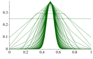
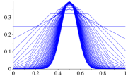
Figure 1: A comparison between Eulerian and binomial distributions for $2,\dots,50$ (magnified by standard variations and normalized into the unit interval). The higher concentration of Eulerian distributions near their mean values is visible.

Such a high concentration in distribution may be ascribed to the large multiplicative factors $k+1$ and $n-k$ when $k$ is near $\frac{1}{2}n$ in (2), leading to the “rich gets richer” effect for terms near the mode of the distribution. More precisely, it is known that $X_{n}$ is asymptotically normally distributed (in the sense of convergence in distribution) with mean asymptotic to $\frac{1}{2}n$ and variance to $\frac{1}{12}n$; the variance is smaller than the binomial variance $\frac{1}{4}n$, which partially reflects the high concentration. For brevity, we will write (CLT standing for central limit theorem)

$$X_{n}\sim\mathscr{N}\bigl{(}{\tfrac{1}{2}n,\tfrac{1}{12}n}\bigr{)}\quad\text{for the CLT}\quad\sup_{x\in\mathbb{R}}\left|\mathbb{P}\left(\frac{X_{n}-\frac{1}{2}n}{\sqrt{\frac{1}{12}n}}\leqslant x\right)-\Phi(x)\right|\to 0,$$ (4)

and $\mathbb{E}(X_{n})\sim\frac{1}{2}n$ and $\mathbb{V}(X_{n})\sim\frac{1}{12}n$, where $\Phi(x)$ denotes the standard normal distribution function

$$\Phi(x):=\frac{1}{\sqrt{2\pi}}\int_{-\infty}^{x}e^{-\frac{1}{2}t^{2}}\,\mathrm{d}{t}\qquad(x\in\mathbb{R}).$$

Such an asymptotic normality with small variance will be constantly observed throughout the examples we will examine.

Due to the multifaceted appearance of Eulerian numbers, it is no wonder that the limit result (4) has been proved by many different approaches in miscellaneous guises; see Table 2 for some of them.

Approach	First reference	Year	See also
Sum of Uniform$[0,1]$	Laplace [158]	1812	[126, 233]
Sum of $\nearrow$ or $\searrow$ indicators	Wolfowitz [241]	1944	[81, 88]
Method of moments	Mann [182]	1945	[72]
Spline & characteristic functions	Curry & Schoenberg [68]	1966	[48, 245]
Real-rootedness	Carlitz et al. [34]	1972	[202, 238]
Complex-analytic	Bender [14]	1973	[100, 133]
Stein’s method	Chao et al. [40]	1996	[58, 62, 107]

Table 2: A list of some approaches used to establish the asymptotic normality (4) of Eulerian numbers.

The normal limit law (4) in the form of descents in permutations appeared first in 1945 by Mann [182] where a method of moments based on the recurrence (2) was employed, proving the empirical observation made in [189]. A similar approach was worked out in David and Barton [72] where they showed that all cumulants of $X_{n}$ are linear with explicit leading coefficients. A more general treatment of runs up and down in permutations had already been given by Wolfowitz [241] in 1944, where he relied instead his analysis on decomposing the random variables $X_{n}$ into a sum of indicators and then on applying Lyapunov’s criteria for CLT by computing the fourth central moments; see [95]. These publications have remained little known in combinatorics literature mainly because they were published in a statistical journal.

On the other hand, the asymptotic normality (4) had been established earlier than 1944 in other forms, although the links to Eulerian numbers were only known later. The earliest connection we found is in Laplace’s Théorie analytique des probabilités, first version published in 1812 [158]. The connection is through the expression (already known to Euler [91, Art. 173])

$$\frac{1}{n!}\,\genfrac{<}{>}{0.0pt}{}{n}{k}=\frac{1}{n!}\sum_{0\leqslant j\leqslant k+1}\binom{n+1}{j}(-1)^{j}(k+1-j)^{n}\qquad(n\geqslant 0),$$

and the distribution of the sum of $n$ independent and identically distributed uniform $[0,1]$ random variables $U_{1},\dots,U_{n}$:

$$\mathbb{P}(U_{1}+\cdots+U_{n}\leqslant t)=\frac{1}{n!}\sum_{0\leqslant j\leqslant t}\binom{n}{j}(-1)^{j}(t-j)^{n}.$$ (5)

It then follows that (see [126, 144, 202, 222, 233])

$$\mathbb{P}(X_{n}\leqslant t)=\mathbb{P}(U_{1}+\cdots+U_{n}\leqslant t+1),$$

and the asymptotic normality of $X_{n}$ follows from that of the sum of uniform random variables, which was first derived by Laplace in [158] by large powers of characteristic functions, Fourier inversion and a saddle-point approximation (or Laplace’s method).

Concerning the expression (5) (the sum on the right-hand side already appeared in [91]), sometimes referred to as Laplace’s formula (see for example [75]), we found that it appears (up to a minor normalization) in Simpson’s 1756 paper [219] where the sum of continuous uniforms is treated as the limit of sum of discrete uniforms; see also his book [220]. The underlying question, closely connected to the counts of repeated tossing of a general dice, has a very long history and rich literature in the early development of probability theory. In particular, Simpson’s treatment finds its roots in de Moivre’s extension of Bernoulli’s binomial distribution, “which in turn was derived from Newton’s binomial theorem and before that from Pascal’s arithmetic triangle—this approach may have the most impressive provenance of any in probability theory” (quoted from Stigler [228, P. 92]). Interestingly, de Moivre’s approach also constitutes one of the very early uses of generating functions; see [228, Ch. 2]. The same expression (5) was derived in the 1770s by Lagrange, Laplace and later by many others, notably in spline and related areas; see [56, 215]. See also the books [95, 122, 200] for more information. Coincidentally, expressions very similar to (5) also emerged in Laplace’s analysis of series expansions; see [157]. But he did not mention the connection to Eulerian numbers.

The sum-of-indicators approach used by Wolfowitz is very useful due to its simplicity but the more classical Lyapunov condition is later replaced by limit theorems for $2$-dependent indicators; see [81, 88, 131]. Also it is possible to derive finer properties such as large deviations; see [88].

Instead of decomposing the Eulerian distribution as a sum of dependent Bernoulli variates, a much more successful and fruitful approach in combinatorics is to express it as a sum of independent Bernoullis based on the property that all roots of its generating polynomial $P_{n}(v)$ (see (1)) are real and negative; see [34, 106, 238]. More precisely, $P_{n}(v)$ has the decomposition [106]

$$P_{n}(v)=\prod_{1\leqslant j\leqslant n}(\zeta_{n,j}+v),$$

where $\zeta_{n,j}\in\mathbb{R}^{+}$. It follows that $X_{n}=\sum_{1\leqslant j\leqslant n}\xi_{n,j}$, where $\xi_{n,j}$ is a Bernoulli with probability $\frac{1}{1+\zeta_{n,j}}$ of assuming $1$. Then Harper’s approach [123] to establishing the asymptotic normality (4) consists in showing that the variance tends to infinity, which amounts to checking Lyapunov’s condition because the summands are bounded. This was carried out for Eulerian distribution by Carlitz et al. in [34]. For a slightly more general context (all roots lying in the negative half-plane), see Hayman’s influential paper [125] and Rényi’s synthesis [206, 207]. See also the surveys [21, 22, 24, 163, 202, 223] for the usefulness of this real-rootedness approach.

We describe two other approaches listed in Table 2 that are closely connected to our study here, leaving aside other ones such as spline functions, matched asymptotics, and Stein’s method; see [40, 48, 58, 62, 68, 107, 115, 245] for more information. For the connection to Pólya’s urn models, see [96, 105, 196] and Section 9.6. See also the very recent papers [108, 150, 149] for a kind of saddle-point approach and [198] for an approach via martingales.

A general study of asymptotic normality based on complex-analytic approach was initiated by Bender [14] where in the particular case of Eulerian numbers he used the relation for the exponential generating function (EGF)

$$F(z,v):=\sum_{n\geqslant 0}\frac{P_{n}(v)}{n!}\,z^{n}=\frac{1-v}{e^{(v-1)z}-v},$$ (6)

and observes that the dominant simple pole $z=\rho(v):=\frac{1}{1-v}\log\frac{1}{v}$ ($\rho(1):=1$) provides the essential information we need for establishing the asymptotic normality (4) since for large $n$

$$\frac{P_{n}(e^{s})}{n!}=e^{-s}\left(\frac{e^{s}-1}{s}\right)^{n+1}+\text{exponentially smaller terms},$$

uniformly for $|s|\leqslant{\varepsilon}$. The uniformity then guarantees that the characteristic functions of the centered and normalized random variables tend to that of the standard normal distribution, implying (4) by Lévy’s continuity theorem (see [99, § C.5]). This approach provides not only a limit theorem, but also much finer properties such as local limit theorems and large deviations in many situations, as already clarified in [14] and later publications such as [100, 109, 133]. In general, the characterization of limit laws or other stochastic properties through a detailed study of the singularities of the corresponding generating functions, coupling with suitable analytic tools, proved very powerful and successful; see [26, 99, 109, 133, 197] for more information. Note that $F$ satisfies the PDE

$$(1-vz)\partial_{z}F-v(1-v)\partial_{v}F=F,$$

the resolution of which adding another interesting dimension to the richness of Eulerian recurrences, which we will briefly explore in Section 3.1.

While each of these approaches has its own strengths and weaknesses, a large portion of the asymptotic normality results for recursively defined polynomials in the combinatorics literature rely on Harper’s real-rootedness approach. Also many powerful criteria for justifying the real-rootedness of a sequence of polynomials have been developed over the years; see for example [21, 22, 24, 163, 202, 223]. However, the real-rootedness property is an exact one and is very sensitive to minor changes. For example, if we change the factor $vn+1-v$ to $vn+(1+v)^{2}$ in the recurrence (1), then all coefficients remain positive but complex roots are abundant as can be seen from Figure 2. On the other hand, by our theorem below, the coefficients still follow the same CLT (4) (with the same asymptotic mean and asymptotic variance). Historically, the proof of the first moment convergence theorem by Markov relies on the (real) zeros of Hermite polynomials; see [104].

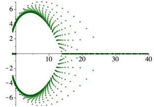
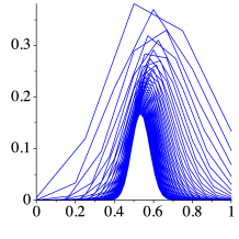
Figure 2: Left: zero distributions of the polynomials $R_{n}(v)=(vn+(1+v)^{2})R_{n-1}(v)+v(1-v)R_{n-1}^{\prime}(v)$ for $n\geqslant 1$ with $R_{0}(v)=1$; right: the corresponding histograms. Here $n=2,3,\dots,50$. The EGF equals $\left(\frac{1-v}{1-ve^{(1-v)z}}\right)^{5}e^{(1-v)z-ve^{(1-v)z}+v}$; see Section 3.1.

On the other hand, the closed-form expression (6) for the EGF represents another exact property and may not be available in more general cases (3), especially when the corresponding PDE is difficult to solve. A simple example is the sequence OEIS A244312 for which

$$P_{n}(v)=\begin{cases}(vn-1)P_{n-1}(v)+v(1-v)P_{n-1}^{\prime}(v),&\text{if $n$ is even},\\ (vn-v)P_{n-1}(v)+v(1-v)P_{n-1}^{\prime}(v),&\text{if $n$ is odd},\end{cases}\qquad(n\geqslant 2),$$ (7)

with $P_{1}(v)=v$. The same $\mathscr{N}\bigl{(}{\frac{1}{2}n,\frac{1}{12}n}\bigr{)}$ can be proved by the method of moments (see Section 4.5), but it is less clear how to solve the corresponding PDE ($F$ being the EGF of $P_{n}$)

$$(1-vz)\partial_{z}F(z,v)+(1-v)\frac{F(z,v)-F(-z,v)}{2}=v(1-v)\partial_{v}F(z,v)+v.$$ (8)

One of our aims of this paper is to show the usefulness of the method of moments for general recurrences such as (3). More precisely, we will derive in the next section a CLT for (3) under reasonably weak conditions on $\alpha(v),\beta(v)$ and $\gamma(v)$. While our limit result seems conceptually less deep (when compared with, say the real-rootedness properties), it is very effective and easy to apply; indeed, its effectiveness will be testified by more than three hundred of polynomials in later sections. The list of examples we compiled is by far the most comprehensive one (although not exhaustive).

On the other hand, although the method of moments has been employed before in similar contexts (see [8, 72, 105, 182]), our manipulation of the recurrence (via developing the “asymptotic transfer”) is simpler and more systematic; see also [135] for the developments for other divide-and-conquer recurrences. In addition to the method of moments, we will also explore the usefulness of the complex-analytic approach for Eulerian recurrences. In particular, we obtain optimal convergence rates in the CLTs, using tools developed in Flajolet and Sedgewick’s authoritative book [99] on Analytic Combinatorics. We will then extend the same method of moments to characterize non-normal limit laws in Sections 6 with applications given in later sections. Extensions along many different directions are discussed in Section 9, and the simpler framework when $\beta(v)=0$ (in (3)) in Section 10 for completeness, some examples of this framework being collected in Appendix B. Section 11 concludes this paper.

Notations. Throughout this paper, $P_{n}(v)$ is a generic symbol whose expression may differ from one occurrence to another, and $Q_{n}(v)$ always denotes the reciprocal polynomial (reading each row coefficients of $P_{n}(v)$ from right to left) of $P_{n}(v)$, except in Section 9.9. The EGF of $P_{n}$ is always denoted by $F(z,v)$. For convenience, the Eulerian recurrence

$$\begin{cases}P_{n}(v)=a_{n}(v)P_{n-1}(v)+b_{n}(v)(1-v)P_{n-1}^{\prime}(v)\qquad(n\geqslant 1)\\ P_{0}(v)\text{ given}\end{cases}$$ (9)

will be abbreviated as $P_{n}\in\mathscr{E}\langle\!\langle a_{n}(v),b_{n}(v)\rangle\!\rangle$ or $P_{n}\in\mathscr{E}\langle\!\langle a_{n}(v),b_{n}(v);P_{0}(v)\rangle\!\rangle$ if we want to specify the initial condition. When the initial condition on $P_{r}(v)$, say $P_{r}(v)=1+v$, is given with $r\geqslant 1$, we write $P_{n}\in\mathscr{E}_{r}\langle\!\langle a_{n}(v),b_{n}(v);1+v\rangle\!\rangle$, with the understanding that the recurrence starts from $n\geqslant r+1$.

Web forms. All examples in this paper (with a total of 628 items in which 594 are in OEIS) are compiled and maintained at the two webpages [137] ((9) with $b_{n}(v)\neq 0$) and [136] ((9) with $b_{n}(v)=0$), with types, links, numerical tables and other properties.

2 A normal limit theorem

We consider in this section the limiting distribution (for large $n$) of the coefficients of linear type Eulerian recurrence $P_{n}(v)$:

$$\mathscr{E}\langle\!\langle\alpha(v)n+\gamma(v),\beta(v);P_{0}(v)\rangle\!\rangle,$$

where $\alpha(v),\beta(v)$, $\gamma(v)$ and $P_{0}(v)$ are any functions analytic in $|v|\leqslant 1$, and we assume that all Taylor coefficients $[v^{k}]P_{n}(v)$ are nonnegative for $k,n\geqslant 0$. If $[v^{k}]P_{n}(v)\geqslant 0$ for $n\geqslant n_{0}$ with $n_{0}>0$, then we can consider the shifted functions $R_{n}(v):=P_{n+n_{0}}(v)$, which satisfy the same form (9) but with $\gamma(v)$ replaced by $n_{0}\alpha(v)+\gamma(v)$. So without loss of generality, we assume that $n_{0}=0$ and $P_{n}(1)>0$ for $n\geqslant 0$ for which a sufficient condition is $[v^{k}]P_{n}(v)\geqslant 0$ and $P_{n}(v)\not\equiv 0$ for $k,n\geqslant 0$.

For simplicity, we write $\alpha=\alpha(1)$ and similarly for $\beta$ and $\gamma$. By (3), we see that

$$P_{n}(1)=(\alpha n+\gamma)P_{n-1}(1)=P_{0}(1)\prod_{1\leqslant j\leqslant n}(\alpha j+\gamma)=P_{0}(1)\alpha^{n}\frac{\Gamma\bigl{(}{n+1+\frac{\gamma}{\alpha}}\bigr{)}}{\Gamma\bigl{(}{1+\frac{\gamma}{\alpha}}\bigr{)}};$$

thus $P_{n}(1)$ is independent of $\beta(v)$, and the factor “$1-v$” in front of $P_{n-1}^{\prime}(v)$ in (9) makes the recurrence satisfied by the moments easier to handle. Note that the assumption that $P_{n}(1)>0$ for $n\geqslant 0$ implies that $\alpha+\gamma>0$.

Define the random variables $X_{n}$ by

$$\mathbb{P}(X_{n}=k)=\frac{[v^{k}]P_{n}(v)}{P_{n}(1)}\qquad(k,n\geqslant 0).$$ (10)

Theorem 1 (Asymptotic normality of $X_{n}$).

Assume that the sequence of functions $P_{n}(v)$ is defined recursively by (9) satisfying (i) $[v^{k}]P_{n}(v)\geqslant 0$ and $P_{n}(v)\not\equiv 0$ for $k,n\geqslant 0$, and (ii) $P_{0}(v)$, $\alpha(v)$, $\beta(v)$ and $\gamma(v)$ analytic in $|v|\leqslant 1$. If, furthermore,

$$\alpha+2\beta>0\quad\text{and}\quad\sigma^{2}>0,$$ (11)

where

$$\mu:=\frac{\alpha^{\prime}(1)}{\alpha+\beta}\quad\text{and}\quad\sigma^{2}:=\mu+\frac{\alpha^{\prime\prime}(1)-2\mu\beta^{\prime}(1)-\alpha\mu^{2}}{\alpha+2\beta},$$ (12)

then the sequence of random variables $X_{n}$, defined by (10), satisfies $X_{n}\sim\mathscr{N}(\mu n,\sigma^{2}n)$, namely, $X_{n}$ is asymptotically normally distributed with the mean and the variance asymptotic to $\mu n$ and $\sigma^{2}n$, respectively.

Indeed, we will prove convergence of all moments.

Observe first that $P_{0}(v)$, $\alpha(v),\beta(v)$ and $\gamma(v)$ need not be polynomials, although in almost all our examples they are; see § 4.5.5 for an example with $\gamma(v)=\frac{1-v}{1+v}$. Also the two constants $\mu$ and $\sigma^{2}$ depend only on $\alpha(v)$ and $\beta(v)$, but not on $\gamma(v)$; neither do they depend on the initial condition $P_{0}(v)$. This offers the flexibility of varying $\gamma(v)$ without changing the normal limit law, as we did in Introduction (Figure 2), provided that $[v^{k}]P_{n}(v)\geqslant 0$. Furthermore, our conditions are very easy to check in all cases we will discuss. Finally, recurrences similar to ours have been studied in the literature; see for example [78, 80, 130, 237] and the references therein.

The same method of proof can be extended to the cases when the factor $\alpha(v)n+\gamma(v)$ of $P_{n-1}(v)$ in (9) also contains higher powers of $n$. See Section 9 for extensions along many different lines.

In connection with the inequalities in (11), we have the order relations for the mean and the variance:

$$\begin{cases}\text{if }\alpha+\beta<0\text{ or }-\frac{\beta}{\alpha}>1,\text{ then }\mathbb{E}(X_{n})\sim Cn^{-\frac{\beta}{\alpha}},\\ \text{if }\alpha+2\beta<0\text{ or }-\frac{\beta}{\alpha}>\frac{1}{2},\text{ then }\mathbb{V}(X_{n})\sim C^{\prime}n^{-\frac{2\beta}{\alpha}},\end{cases}$$

where $C$ and $C^{\prime}$ are constants depending on $P_{0}(v),\alpha(v),\beta(v)$ and $\gamma(v)$. In general, we expect that the limit law is no more normal when $\alpha+2\beta<0$. The same moments approach can be extended to such a case, but we leave this aside in this paper for simplicity of presentation (also because of few examples). For similar contexts in urn models, see [8, 142, 179].

We will prove Theorem 1 by the method of moments. We assume, throughout this section, that $\alpha>0$.

2.1 Mean value of $X_{n}$

Consider now the moment generating function

$$M_{n}(s):=\frac{P_{n}(e^{s})}{P_{n}(1)}.$$

By (9), for $n\geqslant 1$

$$M_{n}(s)=\frac{\alpha(e^{s})n+\gamma(e^{s})}{\alpha n+\gamma}\,M_{n-1}(s)-\frac{\beta(e^{s})(1-e^{-s})}{\alpha n+\gamma}\,M_{n-1}^{\prime}(s),$$ (13)

with $M_{0}(s)=\frac{P_{0}(e^{s})}{P_{0}(1)}$. The mean value can then be computed by the recurrence

$$\mu_{n}:=M_{n}^{\prime}(0)=\left(1-\frac{\beta}{\alpha n+\gamma}\right)\mu_{n-1}+\frac{\alpha^{\prime}(1)n+\gamma^{\prime}(1)}{\alpha n+\gamma}\qquad(n\geqslant 1),$$ (14)

with $\mu_{0}=M_{0}^{\prime}(0)=\frac{P_{0}^{\prime}(1)}{P_{0}(1)}$.

For our asymptotic purpose, we will use the following approximations.

Proposition 1 (Asymptotics of $\mu_{n}$).

The mean $\mu_{n}$ of $X_{n}$ can be approximated as follows.

• If $-\frac{\beta}{\alpha}<1$, then

  $$\mu_{n}=\frac{\alpha^{\prime}(1)}{\alpha+\beta}\,n+\begin{cases}O\bigl{(}{1+n^{-\frac{\beta}{\alpha}}}\bigr{)},&\text{if }\beta\neq 0;\\ O\bigl{(}{\log n}\bigr{)},&\text{if }\beta=0.\end{cases}$$ (15)

• If $-\frac{\beta}{\alpha}=1$, then

  $$\mu_{n}=\frac{\alpha^{\prime}(1)}{\alpha}\,n\log n+C_{0}n+O(\log n),$$

  where ($\psi$ denoting the digamma function)

  $$C_{0}:=\frac{u_{0}\alpha+\gamma^{\prime}(1)}{\alpha+\gamma}-\frac{\alpha^{\prime}(1)}{\gamma}-\frac{\alpha^{\prime}(1)}{\alpha}\left(1+\psi\left(\frac{\gamma}{\alpha}\right)\right).$$

• If $-\frac{\beta}{\alpha}>1$, then

  $$\mu_{n}=C_{1}n^{-\frac{\beta}{\alpha}}\left(1+O\bigl{(}{n^{-1}}\bigr{)}\right)+O(n),$$

  where

  $$C_{1}:=\frac{\Gamma\bigl{(}{1+\frac{\gamma}{\alpha}}\bigr{)}}{\Gamma\bigl{(}{1+\frac{\gamma-\beta}{\alpha}}\bigr{)}}\left(\mu_{0}-\frac{\gamma^{\prime}(1)}{\beta}-\frac{\alpha^{\prime}(1)(\beta-\gamma)}{\beta(\alpha+\beta)}\right).$$

Proof.

We can solve the first-order difference equation (14) and obtain for $n\geqslant 0$:

• if $\beta(\alpha+\beta)\neq 0$, then

  $$\begin{split}\mu_{n}&=\frac{\alpha^{\prime}(1)}{\alpha+\beta}\,n+\frac{\gamma^{\prime}(1)}{\beta}+\frac{\alpha^{\prime}(1)(\beta-\gamma)}{\beta(\alpha+\beta)}\\ &\qquad+\frac{\Gamma\bigl{(}{1+\frac{\gamma}{\alpha}}\bigr{)}\Gamma\bigl{(}{n+1+\frac{\gamma-\beta}{\alpha}}\bigr{)}}{\Gamma\bigl{(}{1+\frac{\gamma-\beta}{\alpha}}\bigr{)}\Gamma\bigl{(}{n+1+\frac{\gamma}{\alpha}}\bigr{)}}\left(\mu_{0}-\frac{\gamma^{\prime}(1)}{\beta}-\frac{\alpha^{\prime}(1)(\beta-\gamma)}{\beta(\alpha+\beta)}\right);\end{split}$$ (16)

• if $\beta=0$, then

  $$\mu_{n}=\frac{\alpha^{\prime}(1)}{\alpha}\,n+\frac{\alpha\gamma^{\prime}(1)-\alpha^{\prime}(1)\gamma}{\alpha^{2}}\left(\psi\left(n+1+\frac{\gamma}{\alpha}\right)-\psi\left(1+\frac{\gamma}{\alpha}\right)\right)+\mu_{0};$$

• if $\alpha+\beta=0$, then

  $$\mu_{n} =(\alpha(n+1)+\gamma)\left(\frac{\alpha^{\prime}(1)}{\alpha^{2}}\left(\psi\left(n+1+\frac{\gamma}{\alpha}\right)-\psi\left(1+\frac{\gamma}{\alpha}\right)\right)+\frac{\mu_{0}}{\alpha+\gamma}\right)$$

  $$\qquad+\left(\frac{\gamma^{\prime}(1)}{\alpha+\gamma}-\frac{\alpha^{\prime}(1)}{\alpha}\right)n.$$

The asymptotic approximations of the Proposition then follow from these relations. Note that $-\frac{\beta}{\alpha}\gtreqqless 1$ is equivalent to $\alpha+\beta\lesseqqgtr 0$. ∎

Corollary 1.

The asymptotic estimate $\mu_{n}\sim\mu n$ is equivalent to $\mu_{n}-\mu_{n-1}\sim\mu$.

Proof.

Note that in general situations $\mu_{n}-\mu_{n-1}\sim\mu$ implies $\mu_{n}\sim\mu n$ but not vice versa. In our setting, this follows from rewriting (14) as

$$\mu_{n}-\mu_{n-1}=-\frac{\beta\mu_{n-1}}{\alpha n+\gamma}+\frac{\alpha^{\prime}(1)n+\gamma^{\prime}(1)}{\alpha n+\gamma},$$

which, by the assumption $\mu_{n}\sim\mu n$, yields

$$\mu_{n}-\mu_{n-1}\sim-\frac{\beta}{\alpha}\,\mu+\frac{\alpha^{\prime}(1)}{\alpha}=\mu.$$

∎

2.2 Recurrence relation for higher central moments

Assume from now on $\alpha+2\beta>0$. Then $\alpha+\beta>0$ (since $\alpha>0$), so that $\mu_{n}$ is linear by (15) with $\mu_{n}-\mu_{n-1}=O(1)$. The higher moments can then be computed through the moment generating function of the centered random variables

$$\hbox to0.0pt{\hskip 2.89581pt\leavevmode\hbox{\set@color$\overline{\hbox{}}$}\hss}{\leavevmode\hbox{\set@color$M$}}_{n}(s):=M_{n}(s)e^{-\mu_{n}s},$$

which, by (13), satisfies the recurrence

$$\hbox to0.0pt{\hskip 2.89581pt\leavevmode\hbox{\set@color$\overline{\hbox{}}$}\hss}{\leavevmode\hbox{\set@color$M$}}_{n}(s) =\frac{e^{-\Delta_{n}s}}{\alpha n+\gamma}\left(\left(\begin{array}[]{l}\alpha(e^{s})n+\gamma(e^{s})\\ -\mu_{n-1}\beta(e^{s})(1-e^{-s})\end{array}\right)\hbox to0.0pt{\hskip 2.89581pt\leavevmode\hbox{\set@color$\overline{\hbox{}}$}\hss}{\leavevmode\hbox{\set@color$M$}}_{n-1}(s)-\beta(e^{s})(1-e^{-s})\,\hbox to0.0pt{\hskip 2.89581pt\leavevmode\hbox{\set@color$\overline{\hbox{}}$}\hss}{\leavevmode\hbox{\set@color$M$}}_{n-1}^{\prime}(s)\right),$$ (19)

for $n\geqslant 1$, where $\Delta_{n}:=\mu_{n}-\mu_{n-1}=O(1)$ by Corollary 1. Write now

$$\hbox to0.0pt{\hskip 2.89581pt\leavevmode\hbox{\set@color$\overline{\hbox{}}$}\hss}{\leavevmode\hbox{\set@color$M$}}_{n}(s)=\sum_{m\geqslant 0}\frac{M_{n,m}}{m!}\,s^{m},$$

where $M_{n,m}=\mathbb{E}(X_{n}-\mu_{n})^{m}$, and

$$e^{-\Delta_{n}s}\alpha(e^{s})=\sum_{j\geqslant 0}\frac{\alpha_{j}}{j!}\,s^{j},\quad e^{-\Delta_{n}s}\beta(e^{s})(1-e^{-s})=\sum_{j\geqslant 1}\frac{\beta_{j}}{j!}\,s^{j},\quad e^{-\Delta_{n}s}\gamma(e^{s})=\sum_{j\geqslant 0}\frac{\gamma_{j}}{j!}\,s^{j},$$ (20)

where all the coefficients depend on $n$ and are bounded. Note that we have the relations $M_{n,0}=1$, $M_{n,1}=0$, $\alpha_{0}=\alpha,\beta_{1}=\beta$ and $\gamma_{0}=\gamma$.

Lemma 1.

The $m$th central moment $M_{n,m}$ of $X_{n}$ satisfies the recurrence

$$M_{n,m}=\left(1-\frac{m\beta}{\alpha n+\gamma}\right)M_{n-1,m}+N_{n,m}\qquad(m\geqslant 2),$$ (21)

where

$$\begin{split}N_{n,m}:=\frac{1}{\alpha n+\gamma}&\left(\sum_{2\leqslant j\leqslant m}\binom{m}{j}\bigl{(}{(\alpha_{j}n+\gamma_{j}-\beta_{j}\mu_{n-1}}\bigr{)}M_{n-1,m-j}\right.\\ &\left.-\sum_{2\leqslant j<m}\binom{m}{j}\beta_{j}M_{n-1,m+1-j}\right).\end{split}$$ (22)

Proof.

By extracting the coefficient of $s^{m}$ on both sides of (19), we obtain (21) with

$$N_{n,m}=\frac{1}{\alpha n+\gamma} \left(\sum_{1\leqslant j\leqslant m}\binom{m}{j}(\alpha_{j}n-\beta_{j}\mu_{n-1}+\gamma_{j})M_{n-1,m-j}\right.$$

$$\left.-\sum_{2\leqslant j<m}\binom{m}{j}\beta_{j}M_{n-1,m+1-j}\right).$$

Since $N_{n,1}=0$, we have the relation

$$\alpha_{1}n-\beta_{1}\mu_{n-1}+\gamma_{1}=(\alpha^{\prime}(1)-\alpha\Delta_{n})n-\gamma\Delta_{n}-\beta\mu_{n-1}+\gamma^{\prime}(1)=0,$$

which is nothing but (14). Then (22) follows. ∎

We now consider the general recurrence

$$x_{n}=\left(1-\frac{m\beta}{\alpha n+\gamma}\right)x_{n-1}+y_{n}\qquad(n\geqslant n_{0}+1),$$ (23)

with $x_{n_{0}}\neq 0$ and $\{y_{n}\}_{n>n_{0}}$ given. Without loss of generality, we assume that

$$j\alpha-m\beta+\gamma\neq 0\qquad(j>n_{0}).$$

If this fails, then we can find a larger $n_{0}$ such that this holds. The solution of this recurrence is easily obtained by iteration.

Lemma 2.

The solution to the recurrence (23) is given by

$$x_{n} =x_{n_{0}}\,\frac{\Gamma\bigl{(}{n_{0}+1+\frac{\gamma}{\alpha}}\bigr{)}\Gamma\bigl{(}{n+1+\frac{\gamma-m\beta}{\alpha}}\bigr{)}}{\Gamma\bigl{(}{n_{0}+1+\frac{\gamma-m\beta}{\alpha}}\bigr{)}\Gamma\bigl{(}{n+1+\frac{\gamma}{\alpha}}\bigr{)}}+\frac{\Gamma\bigl{(}{n+1+\frac{\gamma-m\beta}{\alpha}}\bigr{)}}{\Gamma\bigl{(}{n+1+\frac{\gamma}{\alpha}}\bigr{)}}\sum_{n_{0}<k\leqslant n}\frac{\Gamma\bigl{(}{k+1+\frac{\gamma}{\alpha}}\bigr{)}}{\Gamma\bigl{(}{k+1+\frac{\gamma-m\beta}{\alpha}}\bigr{)}}\,y_{k},$$

for $n\geqslant n_{0}$.

Corollary 2.

Assume $m\geqslant 1$. If $y_{n}\sim cn^{\tau}$, where $c\neq 0$, then

$$x_{n}\sim\begin{cases}\displaystyle\frac{c}{1+\tau+\frac{m\beta}{\alpha}}\,n^{1+\tau},&\text{ if }\tau>-1-\tfrac{m\beta}{\alpha},\\ \displaystyle x_{n_{0}}\frac{\Gamma\bigl{(}{n_{0}+1+\frac{\gamma}{\alpha}}\bigr{)}}{\Gamma\bigl{(}{n_{0}+1+\frac{\gamma-m\beta}{\alpha}}\bigr{)}}\,n^{-\frac{m\beta}{\alpha}},&\text{ if }\tau<-1-\tfrac{m\beta}{\alpha}.\end{cases}$$ (24)

Proof.

By (2) using the asymptotic approximation to the ratio of Gamma functions (see [86, § 1.18])

$$\frac{\Gamma(n+x)}{\Gamma(n+y)}=n^{x-y}\left(1+O\bigl{(}{n^{-1}}\bigr{)}\right),$$ (25)

for large $n$ and bounded $x$ and $y$. ∎

2.3 Asymptotics of $\mathbb{V}(X_{n})$

To prove Theorem 1, we assume that condition (11) holds. Consider the variance. We examine first the term ((22) with $m=2$)

$$N_{n,2}=\frac{\alpha_{2}n+\gamma_{2}-\beta_{2}\mu_{n-1}}{\alpha n+\gamma}\sim\frac{\alpha_{2}-\beta_{2}\mu}{\alpha},$$

where, by the definition (20),

$$\alpha_{2} =\alpha^{\prime\prime}(1)-(2\Delta_{n}-1)\alpha^{\prime}(1)+\Delta_{n}^{2}\alpha,$$

$$\beta_{2} =2\beta^{\prime}(1)-(2\Delta_{n}+1)\beta.$$

Since we assume that $\alpha+2\beta>0$ (condition (11)), we can apply the asymptotic transfer (24) (first case with $\tau=0$), and obtain

$$M_{n,2}=\mathbb{V}(X_{n})\sim\sigma^{2}n,$$

where, by Corollary 1,

$$\sigma^{2}:=\lim_{n\to\infty}\frac{\alpha_{2}-\beta_{2}\mu}{\alpha+2\beta}=\mu+\frac{\alpha^{\prime\prime}(1)-2\mu\beta^{\prime}(1)-\alpha\mu^{2}}{\alpha+2\beta}.$$

Note that the condition $\sigma^{2}>0$ is equivalent to

$$\beta\bigl{(}{\alpha^{\prime\prime}(1)+2\alpha^{\prime}(1)(\alpha^{\prime}(1)+\beta^{\prime}(1))}\bigr{)}>0,$$

because $\alpha+2\beta>0$.

2.4 Asymptotics of higher central moments

We now prove by induction that

$$\left\{\begin{split}M_{n,2\ell}&\sim\frac{(2\ell)!}{\ell!2^{\ell}}\,\sigma^{2\ell}n^{\ell},\\ M_{n,2\ell-1}&=O\bigl{(}{n^{\ell-1}}\bigr{)},\end{split}\right.$$ (26)

for $\ell\geqslant 1$. This will imply particularly that $M_{n,m}=O\bigl{(}{n^{\lfloor\frac{m}{2}\rfloor}}\bigr{)}$ for $m\geqslant 0$. Since (26) with $\ell=1$ has already been proved, we now prove (26) for $\ell\geqslant 2$. Consider first the odd case $m=2\ell+1$. By (22) and induction hypothesis,

$$N_{n,2\ell+1}=O\biggl{(}{\sum_{2\leqslant j\leqslant 2\ell+1}n^{\lfloor\frac{2\ell+1-j}{2}\rfloor}}\biggr{)}=O\bigl{(}{n^{\ell-1}}\bigr{)},$$

implying that $M_{n,2\ell+1}=O\bigl{(}{n^{\ell}}\bigr{)}$. When $m=2\ell$, only the term with $j=2$ in the first sum on the right-hand side of (22) is dominant, and we see that

$$N_{n,2\ell} \sim\binom{2\ell}{2}\frac{\alpha_{2}n-\beta_{2}\mu_{n-1}}{\alpha n}\,M_{n-1,2\ell-2}$$

$$\sim\binom{2\ell}{2}\frac{(2\ell-2)!}{2^{\ell-1}(\ell-1)!}\cdot\frac{\alpha_{2}-\beta_{2}\mu}{\alpha}\,\sigma^{2\ell-2}n^{\ell-1}$$

$$=\frac{(2\ell)!}{2^{\ell}(\ell-1)!}\cdot\frac{\alpha_{2}-\beta_{2}\mu}{\alpha}\,\sigma^{2\ell-2}n^{\ell-1}.$$

By the asymptotic transfer (24) with $m=2\ell$ and $\tau=\ell-1$, we then have

$$M_{n,2\ell}\sim\frac{\alpha_{2}-\beta_{2}\mu}{\ell(\alpha+2\beta)}\cdot\frac{(2\ell)!}{2^{\ell}(\ell-1)!}\,\sigma^{2\ell-2}n^{\ell},$$

which proves the first claim in (26). This completes the proof of (26) and Theorem 1 by Frechet-Shohat’s convergence theorem (see [55, 104]), which, for the reader’s convenience, is included here: it states that if the $k$th moment of a sequence of random variables $Z_{n}$ tends to a finite limit $\nu_{k}$ as $n\to\infty$, and the $\{\nu_{k}\}$’s are the moments of a uniquely determined distribution function $Z$, then $Z_{n}$ converges in distribution to $Z$. This completes the proof of (26), and in turn that of Theorem 1. ∎

From the proof it is obvious that the analyticity of $\alpha(v),\beta(v)$ and $\gamma(v)$ on $|v|\leqslant 1$ can be replaced by that in $|v|<1$ and the existence of all derivatives at unity. This will be needed in Section 4.5.5.

2.5 Mean and variance in a more general setting

In general, for the framework (9) $P_{n}\in\mathscr{E}\langle\!\langle a_{n}(v),b_{n}(v);P_{0}(v)\rangle\!\rangle$, we have

$$P_{n}(1)=P_{0}(1)\prod_{1\leqslant j\leqslant n}a_{j}(1),$$

(assuming each factors positive). Normalizing both sides by $P_{n}(1)$ gives

$$\bar{P}_{n}(v):=\frac{P_{n}(v)}{P_{n}(1)}=\frac{a_{n}(v)}{a_{n}(1)}\bar{P}_{n-1}(v)+\frac{b_{n}(v)}{a_{n}(1)}(1-v)\bar{P}_{n-1}^{\prime}(v).$$

Then the mean $\mu_{n}:=\bar{P}_{n}^{\prime}(1)$ satisfies

$$\mu_{n}=\left(1-\frac{b_{n}(1)}{a_{n}(1)}\right)\mu_{n-1}+\frac{a_{n}^{\prime}(1)}{a_{n}(1)},$$

and the variance $\sigma_{n}^{2}$ satisfies, by the same shifting-the-mean technique used above,

$$\sigma_{n}^{2}=\left(1-\frac{2b_{n}(1)}{a_{n}(1)}\right)\sigma_{n-1}^{2}+\frac{a_{n}^{\prime\prime}(1)+2a_{n}^{\prime}(1)-2b_{n}^{\prime}(1)\mu_{n-1}}{a_{n}(1)}-\Delta_{n}^{2}-\Delta_{n},$$

where $\Delta_{n}:=\mu_{n}-\mu_{n-1}$. These will be used later (see Section 9.8 when $a_{n}(v)$ is not a linear function of $n$).

3 A complex-analytic approach

In addition to the method of moments, which is elementary in nature, we describe briefly a complex-analytic approach in this section, which is equally useful in proving most of the CLTs we derive in this paper but has remained less explored in the combinatorics literature. Following Bender’s pioneering work [14], this approach is based on the EGF $F(z,v)$ of $P_{n}(v)$ (satisfying (9)) and relies on complex analysis (notably the singularity analysis [98]). It turns out that a simple asymptotic framework in the form of quasi-powers [99, § IX.5] [134] proves particularly useful for establishing the asymptotic normality of the coefficients of $P_{n}(v)$.

3.1 The partial differential equation and its resolution

We begin with the PDE satisfied by the EGF of $P_{n}(v)$ (defined in (9))

$$\begin{cases}(1-\alpha(v)z)\partial_{z}F-\beta(v)(1-v)\partial_{v}F-(\alpha(v)+\gamma(v))F=0,\\ F(0,v)=P_{0}(v).\end{cases}$$ (27)

Such a first-order equation can often be solved by the method of characteristics (see [92, 192]), which first reduces a PDE to a family of ordinary DEs and then integrate the solutions with the initial or boundary conditions. For (27), we start with the characteristic equation

$$\frac{\,\mathrm{d}{z}}{1-\alpha(v)z}=-\frac{\,\mathrm{d}{v}}{\beta(v)(1-v)}=\frac{\,\mathrm{d}{F}}{(\alpha(v)+\gamma(v))F}.$$ (28)

The first equation can be written as

$$\frac{\,\mathrm{d}{z}}{\,\mathrm{d}{v}}-\frac{\alpha(v)}{\beta(v)(1-v)}\,z+\frac{1}{\beta(v)(1-v)}=0,$$ (29)

which is not always exactly solvable. In the special case when $\alpha(v)=\beta(v)$ (as in Sections 4 and 5), the above DE becomes

$$(1-v)\frac{\,\mathrm{d}{z}}{\,\mathrm{d}{v}}-z=\frac{\,\mathrm{d}{}}{\,\mathrm{d}{v}}((1-v)z)=-\frac{1}{\beta(v)}.$$

Since $\beta(v)$ is in most cases a polynomial of low degree, this DE can often be solved explicitly. Such a simplification does not apply in general when $\alpha(v)\neq\beta(v)$, but we can still follow the standard procedure to characterize the solution (mostly in implicit forms).

From (29), we see that either we have an ODE of separable type, or we have an explicit form for the integrating factor

$$I(v):=\exp\left(-\int\frac{\alpha(v)}{\beta(v)(1-v)}\,\mathrm{d}{v}\right),$$

the function in the exponent is taken as an antiderivative (or indefinite integral), which is then used to solve the DE (29) by quadrature as

$$\frac{\mbox{d}}{\,\mathrm{d}{v}}\left(I(v)z+\int\frac{I(v)}{\beta(v)(1-v)}\,\,\mathrm{d}{v}\right)=0\Longleftrightarrow\xi(z,v)=C.$$

Here the first integral $\xi(z,v)$ can be made explicit in many cases we study in this paper. For example, when $\alpha(v)=\beta(v)$, we have

$$\xi(z,v)=(1-v)z+\int\frac{\,\mathrm{d}{v}}{\beta(v)},$$ (30)

where the integral is again an antiderivative. We then have the first characteristics, which, after the changes of variables $u=\xi(z,v)$, $w=v$ and $H(u,w)=F(z,v)$, leads to the ODE

$$\frac{\partial}{\partial w}\,H(u,w)+\frac{\alpha(w)+\gamma(w)}{\beta(w)(1-w)}\,H(u,w)=0,$$

which is the second equation of (28). This first-order DE is then solved and we obtain the general relations

$$g(w)H(u,w)=G(u)\Longleftrightarrow g(v)F(z,v)=G(\xi(z,v)),$$

where the integrating factor $g$ has the form

$$g(v)=\exp\left(\int\frac{\alpha(v)+\gamma(v)}{\beta(v)(1-v)}\,\,\mathrm{d}{v}\right).$$

The last step is to specify $G$ by using the initial value at $z=0$:

$$g(v)P_{0}(v)=G(\xi(0,v)).$$

We then conclude that

$$F(z,v)=\frac{G(\xi(z,v))}{g(v)}.$$ (31)

This standard approach works for almost all cases we examine in this paper and has also been used in the combinatorics literature; see for example, [4, 10, 52, 239].

Consider for example the Eulerian recurrence of type $\mathscr{E}\langle\!\langle qvn+p+(qr-p-q)v,qv;1\rangle\!\rangle$; see (37) below. Then we have

$$I(v) =\exp\left(-\int\frac{\,\mathrm{d}{v}}{1-v}\right)=1-v$$

$$g(v) =\exp\left(\int\frac{p(1-v)+qrv}{qv(1-v)}\,\mathrm{d}{v}\right)=v^{\frac{p}{q}}(1-v)^{-r},$$

and, by $P_{0}(v)=1$,

$$G\bigl{(}{q^{-1}\log v}\bigr{)}=g(v),\quad\text{or}\quad G(w)=e^{pw}\bigl{(}{1-e^{qw}}\bigr{)}^{-r}.$$

Finally, by (31),

$$F(z,v)=v^{-\frac{p}{q}}(1-v)^{r}e^{p(1-v)z+\frac{1}{q}\log v}\bigl{(}{1-ve^{q(1-v)z}}\bigr{)}^{-r}=e^{p(1-v)z}\left(\frac{1-v}{1-ve^{q(1-v)z}}\right)^{r}.$$

When the integrals involved have no explicit forms such as the recurrence $\mathscr{E}\langle\!\langle(p+qv)n+1-p-qv,v;1\rangle\!\rangle$ (see [209] or Section 5.2 below), we can still apply the same procedure and get a solution in implicit form:

$$F(z,v)=\frac{1-v}{v}\cdot\frac{T\bigl{(}{S(v)+\frac{(1-v)^{p+q}z}{v^{p}}}\bigr{)}}{1-T\bigl{(}{S(v)+\frac{(1-v)^{p+q}z}{v^{p}}}\bigr{)}},$$ (32)

where $T(S(v))=v$ and

$$S(v)=\int v^{-p-1}(1-v)^{p+q-1}\,\mathrm{d}{v}.$$ (33)

The form (32) is understood in the following formal power series sense:

$$T\left(S(v)+\frac{(1-v)^{p+q}z}{v^{p}}\right)=\sum_{m\geqslant 0}\frac{T^{(m)}(S(v))}{m!}\,\left(\frac{(1-v)^{p+q}}{v^{p}}\right)^{m}z^{m},$$

where $T(S(v))=v$ and $T^{(m)}(S(v))$ are expressible in terms of $S^{(j)}(v)$ for $m,j\geqslant 1$, which in turn are well-specified by

$$S^{\prime}(v)=v^{-p-1}(1-v)^{p+q-1},$$

and then $S^{(m)}=(S^{(m-1)})^{\prime}$ for $m\geqslant 2$.

It is also possible to extend the approach when the non-homogeneous terms are present; see the examples in Sections 5.1.1, 5.2, 5.3, 5.4.1, 5.4.2, 5.5.1, and 5.5.3.

For ease of reference, we list the first integrals $\xi(z,v)$ in Table LABEL:tab-pde for most examples (leading to asymptotic normality) studied in this paper.

Table 3: The first integrals in some exactly solvable cases of (27).

Section	$(\alpha(v),\beta(v))$	$\xi(z,v)$
§ 4	$(qv,qv)$	$(1-v)z+q^{-1}\log v$
§ 5.1	$(qv,v)$	$(1-v)^{q}z+\int v^{-1}(1-v)^{q-1}\,\mathrm{d}{v}$
§ 5.1.1	$(\frac{1}{2}v,v)$	$\sqrt{1-v}z+\frac{1}{2}\log v-\log\bigl{(}{1+\sqrt{1-v}}\bigr{)}$
§ 5.2	$(p+qv,v)$	$\frac{(1-v)^{p+q}}{v^{p}}\,z+\int v^{-p-1}(1-v)^{p+q-1}\,\mathrm{d}{v}$
§ 5.3	$\bigl{(}{\frac{1}{2}(1+v),\frac{1}{2}(3+v)}\bigr{)}$	$\sqrt{(1-v)(3+v)}\,z+2\arcsin(\frac{1}{2}(1+v))$
§ 5.4.1	$(v,1+v)$	$\sqrt{1-v^{2}}\,z+\arcsin(v)$
§ 5.4.1	$(v^{2},v(1+v))$	$\sqrt{1-v^{2}}\,z-\text{arctanh}\bigl{(}{\sqrt{1-v^{2}}}\bigr{)}$
§ 5.4.2	$\bigl{(}{\frac{1}{2}(1+v^{2}),\frac{1}{2}(1+v^{2})}\bigr{)}$	$(1-v)z+2\arctan(v)$
§ 5.4.3	$(v(1+v),v(1+v))$	$(1-v)z+\log\frac{v}{1+v}$
§ 5.4.4	$(2v^{2},v(1+v))$	$(1-v^{2})z-\log v$
§ 5.5.1	$(2qv,q(1+v))$	$(1-v^{2})z-\frac{1}{q}v$
§ 5.5.2	$(2(1+v),3+v)$	$(1-v)(3+v)z+v$
§ 5.5.3	$(q(1+3v),2qv)$	$\frac{(1-v)^{2}}{\sqrt{v}}\,z-\frac{1+v}{q\sqrt{v}}$
§ 5.5.4	$(5+3v,2(1+v))$	$\frac{(1-v)^{2}}{\sqrt{1+v}}\,z-\frac{3+v}{\sqrt{1+v}}$
§ 5.5.5	$(\frac{1}{3}(7+2v),\frac{1}{3}(5+4v)$	$\frac{1-v}{\sqrt{5+4v}}z-\frac{3}{2\sqrt{5+4v}}$
§ 5.5.6	$(1+3v^{2},v(1+v))$	$\frac{(1-v^{2})^{2}}{v}z-\frac{1+v^{2}}{v}$
§ 5.6	$(-1+(q+1)v,qv)$	$v^{\frac{1}{q}}(1-v)z+v^{\frac{1}{q}}$

3.2 Singularity analysis and quasi-powers theorem for CLT

Most EGFs in this paper have either algebraic or logarithmic singularities and it is possible to study the limit laws of the coefficients by examining the singular behavior of the EGF near its dominant singularity; see [14, 109, 100, 133]. The following theorem, from Flajolet and Sedgewick’s book [99, p. 676, § IX.7.2], is very useful for all Eulerian recurrences we study in this paper and leads to a CLT with optimal convergence rate; see also [14] for the original meromorphic version. The proof relies on the uniformity provided by the singularity analysis [98] coupling with the quasi-powers theorems [99, § IX.5].

Notation. For notational convenience, we will write $X_{n}\sim\mathscr{N}\bigl{(}{\mu n,\sigma^{2}n;{\varepsilon}_{n}}\bigr{)}$, which means $X_{n}\sim\mathscr{N}(\mu n,\sigma^{2}n)$ with the convergence rate ${\varepsilon}_{n}$:

$$\sup_{x\in\mathbb{R}}\left|\mathbb{P}\left(\frac{X_{n}-\mu n}{\sigma\sqrt{n}}\leqslant x\right)-\Phi(x)\right|=O({\varepsilon}_{n}),$$

where ${\varepsilon}_{n}\to 0$. The convergence rate in the CLT is often referred to as the Berry-Esseen bound in the probability literature. We will use interchangeably both terms.

Theorem 2 (Algebraic Singularity Schema).

Let $F(z,v)$ be an analytic function at $(z,v)=(0,0)$ with nonnegative coefficients. Under the following three conditions, the random variables $X_{n}$ defined via the coefficients of $F$:

$$\mathbb{E}\bigl{(}{v^{X_{n}}}\bigr{)}:=\frac{[z^{n}]F(z,v)}{[z^{n}]F(z,1)}$$

satisfy $X_{n}\sim\mathscr{N}(\mu n,\sigma^{2}n;n^{-\frac{1}{2}})$, where the convergence rate is, modulo the implied constant, optimal. The three conditions are:

1. Analytic perturbation: there exist three functions $\Lambda,K,\Psi$, analytic in a domain $D:=\{|z|\leqslant\zeta\}\times\{|v-1|\leqslant{\varepsilon}\}$, such that, for some $\zeta_{0}$ with $0<\zeta_{0}\leqslant\zeta$, and ${\varepsilon}>0$, the following representation holds, $\kappa\not\in\mathbb{Z}_{\leqslant 0}$,

   $$F(z,v)=\Lambda(z,v)+K(z,v)\Psi(z,v)^{-\kappa};$$ (34)

   furthermore, assume that, in $|z|\leqslant\zeta$, there exists a unique root $\rho>0$ of the equation $\Psi(z,1)=0$, that this root is simple, and that $K(\rho,1)\not=0$.

2. Non-degeneracy: one has $\partial_{z}\Psi(\rho,1)\cdot\partial_{v}\Psi(\rho,1)\neq 0$, ensuring the existence of a non-constant $\rho(v)$ analytic at $v=1$, such that $\Psi(\rho(v),v)=0$ and $\rho(1)=\rho$.

3. Variability: $\sigma^{2}(\rho):=\frac{\rho^{\prime\prime}(1)}{\rho(1)}+\frac{\rho^{\prime}(1)}{\rho(1)}-\bigl{(}{\frac{\rho^{\prime}(1)}{\rho(1)}}\bigr{)}^{2}\neq 0$.

For our purpose, we show how the two constants $(\mu,\sigma^{2})$ can be computed from the dominant singularity $\rho(v)$. By the asymptotic approximation (see [99, Eq. (64), p. 678])

$$[z^{n}]F(z,v)=g(v)n^{\kappa-1}\rho(v)^{-n}\left(1+O\bigl{(}{n^{-1}}\bigr{)}\right),$$ (35)

where the $O$-term holds uniformly in a neighborhood of $v=1$, we see that

$$\mathbb{E}\bigl{(}{v^{X_{n}}}\bigr{)}=\frac{g(v)}{g(1)}\,\exp\left(n\log\frac{\rho(1)}{\rho(v)}\right)\left(1+O\bigl{(}{n^{-1}}\bigr{)}\right),$$

uniformly for $|v-1|\leqslant{\varepsilon}$. Thus

$$\mu=-[s]\log\rho(e^{s})=-\frac{\rho^{\prime}(1)}{\rho}\quad\text{and}\quad\sigma^{2}(\rho)=2[s^{2}]\log\rho(e^{s}).$$ (36)

Note also that

$$\rho^{\prime}(1)=-\frac{\partial_{v}\Psi(\rho,1)}{\partial_{z}\Psi(\rho,1)},$$

and it is often simpler to replace the second condition (of the Theorem) by $\rho^{\prime}(1)\neq 0$ or $\mu\neq 0$.

We illustrate the use of these expressions by the simplest example when $F$ has the form (see (38))

$$F(z,v)=e^{p(1-v)z}\left(\frac{1-v}{1-ve^{q(1-v)z}}\right)^{r},$$

where $q,r>0$ and $p\leqslant qr$ (implying that $[z^{n}v^{k}]F(,v)\geqslant 0$). With the notations of (34), we take $\kappa=r$, $\Lambda=0$, $K(z,v)=e^{p(1-v)z}$ and

$$\Psi(z,v):=\frac{1-ve^{q(1-v)z}}{1-v}.$$

Then the dominant singularity $\rho(v)$ solves the equation $1=ve^{q(1-v)z}$ and $\rho(1)=q^{-1}$, namely,

$$\rho(v)=\frac{\log v}{q(v-1)}.$$

One checks that $-\rho^{\prime}(1)=\frac{1}{2q}\neq 0$. Also by the Taylor expansion

$$-\log\rho(e^{s}) =\log q+\frac{s}{2}+\sum_{k\geqslant 1}\frac{\text{Bernoulli}_{2k}}{(2k)\cdot(2k)!}\,s^{2k}$$

$$=\log q+\frac{s}{2}+\frac{s^{2}}{24}-\frac{s^{4}}{2880}+\frac{s^{6}}{181400}+O\bigl{(}{|s|^{8}}\bigr{)},$$

we then obtain $(\mu,\sigma^{2})=\bigl{(}{\frac{1}{2},\frac{1}{12}}\bigr{)}$. We see that the variance constant does not require the calculation of the second moment and the square of the mean, making it a cancellation-free approach for computing the variance; see [133] for more information on quasi-powers framework. Furthermore, finer results such as cumulants of higher orders and more effective asymptotic approximations can be derived. For example, in the above case, we see that all odd cumulants are bounded, and all even cumulants are asymptotically linear; in particular, the fourth and sixth cumulants are asymptotic to $-\frac{1}{120}n$ and $\frac{1}{252}n$, respectively.

In Table LABEL:tab-qp, we list the mean and the variance constants of a few cases to be discussed below.

Table 4: The dominant singularity $\rho(v)$ and the corresponding mean and variance constants in some exactly solvable cases of (27). Here $(\star)=\bigl{(}{\frac{q}{p+q+1},\frac{q(p+1)(p+q)}{(p+q+1)^{2}(p+q+2)}}\bigr{)}$; see § 5.2.

Section	$(\alpha(v),\beta(v))$	$F(z,v)$	$\rho(v)$	$(\mu,\sigma^{2})$
§ 4	$(qv,qv)$	(38)	$\frac{\log v}{q(v-1)}$	$\bigl{(}{\frac{1}{2},\frac{1}{12}}\bigr{)}$
§ 5.1	$(qv,v)$	(48)	$\frac{\int_{v}^{1}t^{-1}(1-t)^{q-1}\,\mathrm{d}{t}}{(1-v)^{q}}$	$\bigl{(}{\frac{q}{q+1},\frac{q^{2}}{(q+1)^{2}(q+2)}}\bigr{)}$
§ 5.1.1	$(v,2v)$	(52)	$\frac{1}{2\sqrt{1-v}}\log\frac{1+\sqrt{1-v}}{1-\sqrt{1-v}}$	$\bigl{(}{\frac{1}{3},\frac{2}{45}}\bigr{)}$
§ 5.2	$(p+qv,v)$	(32)	$\frac{\int_{v}^{1}t^{-p-1}(1-t)^{p+q-1}\,\mathrm{d}{t}}{v^{-p}(1-t)^{p+q}}$	$(\star)$
§ 5.3	$\bigl{(}{\frac{1}{2}(1+v),\frac{1}{2}(3+v)}\bigr{)}$	(59)	$\frac{2\arccos\frac{1+v}{2}}{\sqrt{(1-v)(3+v)}}$	$\bigl{(}{\frac{1}{6},\frac{23}{180}}\bigr{)}$
§ 5.4.1	$(v,1+v)$	(62)	$\frac{\arccos(v)}{\sqrt{1-v^{2}}}$	$\bigl{(}{\frac{1}{3},\frac{8}{45}}\bigr{)}$
§ 5.4.1	$(v^{2},v(1+v))$	(62)	$\frac{\log(1+\sqrt{1-v^{2}})-\log v}{\sqrt{1-v^{2}}}$	$\bigl{(}{\frac{2}{3},\frac{8}{45}}\bigr{)}$
§ 5.4.2	$\bigl{(}{\frac{1}{2}(1+v^{2}),\frac{1}{2}(1+v^{2})}\bigr{)}$	(66)	$\frac{\arccos\bigl{(}{\frac{2v}{1+v^{2}}}\bigr{)}}{v-1}$	$\bigl{(}{\frac{1}{2},\frac{5}{12}}\bigr{)}$
§ 5.4.3	$(v(1+v),v(1+v))$	(68)	$\frac{1}{1-v}\log\frac{1+v}{2v}$	$\bigl{(}{\frac{3}{4},\frac{7}{48}}\bigr{)}$
§ 5.4.4	$(2v^{2},v(1+v))$	(70)	$\frac{-\log v}{1-v^{2}}$	$\bigl{(}{1,\frac{1}{3}}\bigr{)}$
§ 5.5.1	$(2qv,q(1+v))$	(73)	$\frac{1}{q(1+v)}$	$\bigl{(}{\frac{1}{2},\frac{1}{4}}\bigr{)}$
§ 5.5.2	$(2(1+v),3+v)$	(75)	$\frac{1}{3+v}$	$\bigl{(}{\frac{1}{4},\frac{3}{16}}\bigr{)}$
§ 5.5.3	$(q(1+3v),2qv)$	(77)	$\frac{1}{q(1+\sqrt{v})^{2}}$	$\bigl{(}{\frac{1}{2},\frac{1}{8}}\bigr{)}$
§ 5.5.4	$(5+3v,2(1+v))$	(78)	$\frac{1}{(\sqrt{2}+\sqrt{1+v})^{2}}$	$\bigl{(}{\frac{1}{4},\frac{5}{32}}\bigr{)}$
§ 5.5.5	$(\frac{1}{3}(7+2v),\frac{1}{3}(5+4v)$	(79)	$\frac{2}{3+\sqrt{5+4v}}$	$\bigl{(}{\frac{1}{9},\frac{2}{27}}\bigr{)}$
§ 5.5.6	$(1+3v^{2},v(1+v))$	(80)	$\frac{1}{(1+v)^{2}}$	$\bigl{(}{1,\frac{1}{2}}\bigr{)}$
§ 5.6	$(-1+(q+1)v,qv)$	(81)	$\frac{v^{-\frac{1}{q}}-1}{1-v}$	$\bigl{(}{\frac{q+1}{2q},\frac{q^{2}-1}{12q^{2}}}\bigr{)}$

In the next two sections (and in Section 9), we will apply both Theorem 1 and Theorem 2 to polynomials whose coefficients follow asymptotically normal limit laws. The main differences between the two theorems when specializing to Eulerian recurrences are similar to those between an elementary and an analytic approach to asymptotics (see [50, 197]): Theorem 1 is more general but gives weaker results, while Theorem 2 gives stronger approximations but needs the availability of tractable EGFs (often from solving the corresponding PDEs). Note that both theorems are not limited to Eulerian recurrences.

	Theorem  1	Theorem 2
nature	elementary	complex-analytic
based on	recurrence (9)	generating function
CLT	no rate	with optimum rate

4 Applications I: $(\alpha(v),\beta(v))=(qv,qv)\Longrightarrow\mathscr{N}\bigl{(}{\frac{1}{2}n,\frac{1}{12}n}\bigr{)}$

We gather in this section many applications of Theorems 1 and 2, grouping them according to the pair $(\alpha(v),\beta(v))=(qv,qv)$; other pairs with $\alpha(v)\neq\beta(v)$ or nonlinear $\alpha(v),\beta(v)$ are further categorized in the next section. Despite our efforts to be comprehensive, omissions may still remain in view of the large literature on Eulerian numbers and their applications.

Before our discussions, we observe that the following three simple transformations on polynomials do not change essentially the distribution of the coefficients:

• shift: $P_{n}(v)\mapsto P_{n+m}(v)$,

• translation: $P_{n}(v)\mapsto v^{m}P_{n}(v)$, and

• reciprocity (or row-reverse): $P_{n}(v)\mapsto Q_{n}(v):=v^{n+m}P_{n}\bigl{(}{\frac{1}{v}}\bigr{)}$, where $m$ is properly chosen so that $Q_{n}(v)$ is a polynomial in $v$ and is referred to as the reciprocal polynomial of $P_{n}$.

In particular, the polynomials $Q_{n}(v):=v^{n+m}P_{n}(\frac{1}{v})$ of $P_{n}$ (defined in (9)) satisfy the recurrence

$$Q_{n}\in\mathscr{E}\left\langle\!\left\langle\left(v\alpha\bigl{(}{\tfrac{1}{v}}\bigr{)}-v(1-v)\beta\bigl{(}{\tfrac{1}{v}}\bigr{)}\right)n+v\gamma\bigl{(}{\tfrac{1}{v}}\bigr{)}-(m-1)v(1-v)\beta\bigl{(}{\tfrac{1}{v}}\bigr{)},v^{2}(1-v)\beta\bigl{(}{\tfrac{1}{v}}\bigr{)}\right\rangle\!\right\rangle.$$

Note specially that if $X_{n}$ (and $Y_{n}$) is defined by the coefficients of $P_{n}$ (and $Q_{n}$) as in (10), then $X_{n}+Y_{n}=n+m$. These operations sometimes provide additional computational efficiencies. In particular, we may assume in many cases that $P_{0}(v)=1$ and start the recurrence (9) from $n=1$.

For an easier classification of the examples, we introduce further the following definition.

Definition 1 (Equivalence of distributions).

Two random variables $X_{n}$ and $Y_{n}$ are said to be equivalent (or have the same distribution) if $X_{n}+dY_{n+m}=c_{n}$ for $n\geqslant n_{0}$ for some constant $d\neq 0$, integers $m$ and $n_{0}$ and a deterministic sequence $c_{n}$.

Eulerian numbers are the source prototype of our framework (9), and we saw in Introduction that they satisfy (9) with $\alpha(v)=\beta(v)=v$. Theorem 1 applies since $\alpha=\beta=\alpha^{\prime}(1)=\beta^{\prime}(1)=1$, and, by (12), $\mu=\frac{1}{2}$ and $\sigma^{2}=\frac{1}{12}$. The literature abounds with diverse extensions and generalizations of Eulerian numbers. It turns out that exactly the same limiting $\mathscr{N}\bigl{(}{\frac{1}{2}n,\frac{1}{12}{n}}\bigr{)}$ behavior appears in a large number of variants, extensions, and generalizations of Eulerian numbers (by a direct application of Theorem 1), which we examine below. Furthermore, in almost all cases, the stronger result $\mathscr{N}\bigl{(}{\frac{1}{2}n,\frac{1}{12}{n};n^{-\frac{1}{2}}}\bigr{)}$ also follows from a direct use of Theorem 2.

4.1 The class $\mathscr{A}(p,q,r)$

One of the most common patterns we found with very rich combinatorial properties among the extensions of Eulerian numbers is of the form

$$P_{n}\in\mathscr{E}\langle\!\langle qvn+p+(qr-q-p)v,qv;1\rangle\!\rangle,$$ (37)

which covers more than 60 examples in OEIS (and many other non-OEIS ones) and leads always to the same $\mathscr{N}\bigl{(}{\frac{1}{2}n,\frac{1}{12}n;n^{-\frac{1}{2}}}\bigr{)}$ behavior. The EGF of $P_{n}$ satisfies the PDE

$$(1-qvz)\partial_{z}F-qv(1-v)\partial_{v}F=(p+(qr-p)v)F,$$

with $F(0,v)=1$, which has the closed-form solution (see Section 3.1)

$$F(z,v)=e^{p(1-v)z}\left(\frac{1-v}{1-ve^{q(1-v)z}}\right)^{r}.$$ (38)

For convenience, we will write this form as $F\in\mathscr{A}(p,q,r)$. We also write $c\mathscr{A}(p,q,r)$ to denote the class of polynomials whose EGFs are of the form $cF(z,v)$. Although it is possible to restrict our consideration to only the case $q=1$ by a simple change of variables, we keep the form of three parameters ($p,q,r$) for a more natural presentation of the diverse examples.

For later reference, we state the following result.

Theorem 3.

Assume that the EGF $F$ of $P_{n}$ is of type $F\in\mathscr{A}(p,q,r)$. If $q,r>0$ and $0\leqslant p\leqslant qr$, then the random variables $X_{n}$ defined on the coefficients of $P_{n}$ ((10)) satisfies $X_{n}\sim\mathscr{N}\bigl{(}{\frac{1}{2}n,\frac{1}{12}n;n^{-\frac{1}{2}}}\bigr{)}$. More precise approximations to the mean and the variance are given by

$$\mathbb{E}(X_{n})=\frac{n+r}{2}-\frac{p}{q}+O(n^{-1}),\;\text{ and }\;\mathbb{V}(X_{n})=\frac{n+r}{12}+O(n^{-2}).$$ (39)

Proof.

Observe that $q,r>0$ and $p\leqslant qr$ imply $P_{n}(1)>0$ for $n\geqslant 0$ and $[v^{k}]P_{n}(v)\geqslant 0$ for $k,n\geqslant 0$. The CLT without rate $\mathscr{N}\bigl{(}{\frac{1}{2}n,\frac{1}{12}n}\bigr{)}$ follows easily from Theorem 1. The stronger version with optimal rate is proved by applying Theorem 2 (as already discussed in Section 3.2). The finer estimates for $\mathbb{E}(X_{n})$ and $\mathbb{V}(X_{n})$ are obtained by a direct calculation using either the recurrence $\mathscr{E}\langle\!\langle qvn+p+(qr-q-p)v,qv;1\rangle\!\rangle$ or the EGF (by computing $[z^{n}t]F(z,1+t)$ for the mean and $2[z^{n}t^{2}]F(z,1+t)$ for the second factorial moment). Note specially the smaller error term in the variance approximation in (39); also when $r=1$, both $O$-terms in (39) are identically zero for $n\geqslant 2$. ∎

Lemma 3.

If $F\in\mathscr{A}(p,q,r)$, then $\stackrel{{\scriptstyle\leftarrow}}{{F}}\in\mathscr{A}(qr-p,q,r)$, where $\stackrel{{\scriptstyle\leftarrow}}{{F}}(z,v):=F(vz,\frac{1}{v})$ denotes the EGF of the reciprocal polynomial of $P_{n}$, and if $p=qr$, then $\partial_{z}F\in p\mathscr{A}(p,q,r+1)$.

The proof is straightforward and omitted. Note that $\partial_{z}F$ corresponds to the EGF of $P_{n+1}$.

Corollary 3.

If $F\in\mathscr{A}(p,q,r)$ with $p=\frac{1}{2}qr$, then $P_{n}$ is symmetric or palindromic, namely, $P_{n}(v)=v^{n}P_{n}\bigl{(}{\frac{1}{v}}\bigr{)}$.

Definition 2.

We write $X_{n}(p,q,r)\stackrel{{\scriptstyle d}}{{\thickapprox}}X_{n}(p^{\prime},q^{\prime},r^{\prime})$ if the random variables associated with the two types $\mathscr{A}(p,q,r)$ and $\mathscr{A}(p^{\prime},q^{\prime},r^{\prime})$ (defined as in (10)), respectively, are equivalent in the sense of Definition 1.

Corollary 4.

If $p\neq qr$, then $X_{n}(p,q,r)\stackrel{{\scriptstyle d}}{{\thickapprox}}X_{n}(qr-p,q,r)$; if $p=qr$, then

$$X_{n}(qr,q,r)\stackrel{{\scriptstyle d}}{{\thickapprox}}X_{n}(0,q,r)\stackrel{{\scriptstyle d}}{{\thickapprox}}X_{n}(qr,q,r+1)\stackrel{{\scriptstyle d}}{{\thickapprox}}X_{n}(q,q,r+1).$$ (40)

This shows partly the advantages of considering the framework (37) and the EGF (38).

We now discuss some concrete examples grouped according to increasing values of $q$. Most CLTs and their optimal Berry-Esseen bounds are new.

4.2 $q=1$

Eulerian numbers

By (6), the Eulerian numbers are of type $\mathscr{A}(1,1,1)$, and, by Lemma 3, also of types $\mathscr{A}(1,1,2)$ and $\mathscr{A}(0,1,1)$. The correspondence to OEIS sequences is as follows.

Description	OEIS	Type (in $\mathscr{A}$)	Type (in $\mathscr{E}$)
Eulerian numbers ($1\leqslant k\leqslant n$)	A008292	$\mathscr{A}(0,1,1)-1$	$\mathscr{E}_{1}\langle\!\langle vn,v;v\rangle\!\rangle$
Eulerian numbers ($1\leqslant k\leqslant n$)	A123125	$\mathscr{A}(0,1,1)$	$\mathscr{E}\langle\!\langle vn,v;1\rangle\!\rangle$
Eulerian numbers ($0\leqslant k<n$)	A173018	$\mathscr{A}(1,1,1)$	$\mathscr{E}\langle\!\langle vn+1-v,v;1\rangle\!\rangle$

Note that $v\mathscr{A}(1,1,1)=\mathscr{A}(0,1,1)+v-1$. In addition to these, with $P_{n}$ defined by A123125, the sequence A113607 equals $v^{n+1}+1+P_{n}(v)$ (with $1$’s at both ends of each row); we obtain the same CLT.

LI Shanlan numbers

LI Shanlan (1810–1882) in his 1867 book Duoji Bilei [160, Ch. 4] (Series Summations by Analogies) studied $\mathscr{A}(1,1,r+1)$, where $r=0,1,\dots$; see [165, 246] (in Chinese), [184, p. 350], and [240, Part II] for more modern accounts. In our format, $P_{n}$ satisfies

$$P_{n}\in\mathscr{E}\langle\!\langle vn+1+(r-1)v,v;1\rangle\!\rangle.$$ (41)

The first few rows of these LI Shanlan numbers are given in Table 5.

$n\backslash k$	$0$	$1$	$2$	$3$	$4$
$0$	$1$
$1$	$1$	$r$
$2$	$1$	$1+3r$	$r^{2}$
$3$	$1$	$4+7r$	$1+4r+6r^{2}$	$r^{3}$
$4$	$1$	$11+15r$	$11+30r+25r^{2}$	$1+5r+10r^{2}+10r^{3}$	$r^{4}$

Table 5: The first few rows of the polynomial $\mathscr{E}\langle\!\langle vn+1+(r-1)v,v;1\rangle\!\rangle$.

Indeed, LI derived in [160] the identity

$$\sum_{1\leqslant j\leqslant m}j^{n}\binom{j+r-1}{j-1}=\sum_{0\leqslant k\leqslant n}\binom{m+n-k+r}{m-1-k}[v^{k}]P_{n}(v)$$

only for $n=1,2,3$ (generalizing a version of the identity later often named after Worpitzky [242]), and mentioned the straightforward extension to higher powers, which was later carried out in detail by Zhang [246], who also obtained many interesting expressions for $P_{n}(v)$.

By Corollary 4, we see that

$$X_{n}(1,1,r+1)\stackrel{{\scriptstyle d}}{{\thickapprox}}X_{n}(0,1,r)\stackrel{{\scriptstyle d}}{{\thickapprox}}X_{n}(r,1,r)\stackrel{{\scriptstyle d}}{{\thickapprox}}X_{n}(r,1,r+1).$$ (42)

Also by a change of variables, we have for any $p>0$

$$X_{n}(1,1,r+1)\stackrel{{\scriptstyle d}}{{\thickapprox}}X_{n}(p,p,r+1).$$ (43)

In particular, the cases $r=0,1$ correspond to Eulerian numbers (so that $\mathscr{A}(2,2,2)$ also leads to the same Eulerian distribution A008292), and the cases $r=2,\dots,5$ appear in OEIS with suitable offsets (see the table below), where they are referred to as $r$-Eulerian numbers whose generating polynomials satisfy $P_{n}\in\mathscr{E}_{r}\langle\!\langle vn+1-v,v;1\rangle\!\rangle$, which equals (41) by shifting $n$ to $n-r$; see also Section 4.5.2.

Description	OEIS	Type	Equivalent types
$2$-Eulerian	A144696	$\mathscr{A}(1,1,3)$	$\mathscr{A}(0,1,2)$, $\mathscr{A}(2,1,2),\mathscr{A}(2,1,3)$
$3$-Eulerian	A144697	$\mathscr{A}(1,1,4)$	$\mathscr{A}(0,1,3)$, $\mathscr{A}(3,1,3),\mathscr{A}(3,1,4)$
$4$-Eulerian	A144698	$\mathscr{A}(1,1,5)$	$\mathscr{A}(0,1,4)$, $\mathscr{A}(4,1,4),\mathscr{A}(4,1,5)$
$5$-Eulerian	A144699	$\mathscr{A}(1,1,6)$	$\mathscr{A}(0,1,5)$, $\mathscr{A}(5,1,5),\mathscr{A}(5,1,6)$
$6$-Eulerian	A152249	$\mathscr{A}(1,1,7)$	$\mathscr{A}(0,1,6)$, $\mathscr{A}(6,1,6),\mathscr{A}(6,1,7)$

These numbers found their later use in data smoothing techniques; see [188, §4.3]. For more information on $r$-Eulerian numbers, see [18, 171, 185] and the corresponding OEIS pages. Combinatorial interpretation of the polynomials of type $\mathscr{A}(1,1,r)$ was discussed by Carlitz in [30]; these polynomials were also examined in the recent paper [39] (without mentioning Eulerian numbers). The distribution associated with $\mathscr{A}(0,1,p)$ appeared in [77] and later in a random walk model [141].

The type $\mathscr{A}(q,1,q)$ (switching from $r$ to $q$ for convention) has also been studied in the combinatorics literature, corresponding to the recurrence satisfied by the $q$-analogue of Eulerian numbers ($\mathcal{S}_{n}$ being the set of all permutations of $n$ elements)

$$P_{n}(v)=\sum_{\pi\in\mathcal{S}_{n}}q^{\text{cycle}(\pi)}v^{\text{exceedance}(\pi)+1},$$

which is of type

$$P_{n}\in\mathscr{E}\langle\!\langle vn+q-v,v;1\rangle\!\rangle;$$ (44)

see Foata and Schützenberger’s book [101, Ch. IV] for a detailed study. See also [208, p. 235] and [28, 77, 139, 178]. The type $\mathscr{A}(2,1,1)$ (with the different initial condition $P_{2}(v)=2$) enumerates big ($\geqslant 2$) descents in permutations:

Big descents in perms.	A120434	$\mathscr{A}(2,1,2)$	$\mathscr{E}_{1}\langle\!\langle vn+2-v,v;2\rangle\!\rangle$
Reciprocal of A120434	A199335	$\mathscr{A}(0,1,2)$	$\mathscr{E}\langle\!\langle vn+v,v;1\rangle\!\rangle$

As already indicated above, these two distributions are also equivalent to those of $2$-Eulerian numbers and of $\mathscr{A}(2,1,3)$.

By Theorem 3, the polynomials (44) with any real $q>0$ lead to the same $\mathscr{N}\bigl{(}{\frac{1}{2}n,\frac{1}{12}n;n^{-\frac{1}{2}}}\bigr{)}$ asymptotic behavior.

Generalized Eulerian numbers [37, 190]

Morisita [190] introduced in 1971 in statistical ecology a class of distributions, which corresponds to $\mathscr{A}(p,1,p+q)$ in our notation, or

$$P_{n}\in\mathscr{E}\langle\!\langle vn+p+(q-1)v,v;1\rangle\!\rangle.$$ (45)

By Corollary 4, $X_{n}(p,1,p+q)\stackrel{{\scriptstyle d}}{{\thickapprox}}X_{n}(q,1,p+q)$. Such polynomials were also independently studied in 1974 by Carlitz and Scoville [37], and are referred to as the generalized Eulerian numbers; see [42, 140, 141].

The CLT for the coefficients of (45) was later derived in [42] in a statistical context by checking the real-rootedness property and Lindeberg’s condition, as motivated by [140, 190], where the usefulness of these numbers is further highlighted via a few concrete models. See also [141] for more models leading to $X_{n}(p,1,p+q)$.

In the context of random staircase tableaux, these polynomials were also examined in detail by Hitczenko and Janson [128], where they derived not only a CLT but also an LLT. Moreover, they also address the situation when $p$ and $q$ may become large with $n$.

Euler-Frobenius numbers

Dwyer [82] studied $\mathscr{A}(p,1,1)$, referred to as the “cumulative numbers” but better known later as the Euler-Frobenius numbers; see for example [111, 124, 144, 208] and the references therein. They are called non-central Eulerian numbers in [44, p. 538]. The coefficients of such polynomials are nonnegative if $p\in[0,1]$; see also [102, 147]. The asymptotic normality $\mathscr{N}\bigl{(}{\frac{1}{2}n,\frac{1}{12}n}\bigr{)}$ of the coefficients is first proved in [124] and later in [59, 111, 144] by different approaches; see also [111, 124, 133, 144] for local limit theorems. In particular, an asymptotic expansion for $p=0$ (Eulerian numbers) was derived in the Ph.D. Thesis of the first author [133, p. 76], the approach there being based on a framework of quasi-powers [99, 134] and a direct Fourier analysis.

This class of polynomials is more useful than it seems because the coefficients of any polynomial of type $\mathscr{A}(p,q,1)$ with $q>0$ have the same distribution as $\mathscr{A}(\frac{p}{q},1,1)$, which has nonnegative coefficients when $0\leqslant p\leqslant q$; see [144] for details.

4.3 $q=2$

Eulerian numbers

The sequence of polynomials A296229, which corresponds to $2^{n}\genfrac{<}{>}{0.0pt}{}{n}{k}$, is of type (shifting $n$ by $1$) $2\mathscr{A}(2,2,2)$, which has the same distribution as Eulerian numbers; see (43).

MacMahon numbers (or Eulerian numbers of type $B$)

MacMahon numbers (first introduced in [177]) are generated by the recurrence $P_{n}\in\mathscr{E}\langle\!\langle 2vn+1-v,2v;1\rangle\!\rangle$, which is of type $\mathscr{A}(1,2,1)$; see Figure 3. Their signed version is A138076, and a doubled-power version (with a zero between every two entries) is A158781. The CLT $\mathscr{N}\bigl{(}{\frac{1}{2}n,\frac{1}{12}n}\bigr{)}$ was proved in [49, 71, 144]; see also [76, 214]. The stronger results $\mathscr{N}\bigl{(}{\frac{1}{2}n,\frac{1}{12}n;n^{-\frac{1}{2}}}\bigr{)}$ for these numbers follow readily from Theorem 3.

Eulerian numbers of type $B$	A060187	$\mathscr{A}(1,2,1)$	$\mathscr{E}\langle\!\langle 2vn+1-v,2v;1\rangle\!\rangle$
A060187: $v\mapsto v^{2}$	A158781		$\mathscr{E}\langle\!\langle 2v^{2}n+1-v^{2},v(1+v);1\rangle\!\rangle$
Signed version of A060187	A138076

The signed version A138076 can on the other hand be generated by $P_{0}(v)=1$ and

$$P_{n}(v)=(2vn-1-v)P_{n-1}(v)-2v(1+v)P_{n-1}^{\prime}(v)\qquad(n\geqslant 1),$$

whose EGF has the closed form expression $\mathscr{A}(1,2,1)$ but with $v\mapsto-v$ and $z\mapsto-z$.

Polynomials arising from higher order derivatives

Many polynomials of the Eulerian type (9) are generated by successive differentiations of a given base function. Indeed, this is the very first genesis of Eulerian numbers (see [91]):

$$(x\mathbb{D}_{x})^{n}\frac{1}{1-x}=\frac{P_{n}(x)}{(1-x)^{n+1}},\quad\text{where }P_{n}\text{ is of type }\mathscr{A}(0,1,1).$$

For type $B$

$$\mathbb{D}_{x}^{n}\frac{e^{x}}{1-e^{2x}}=\frac{e^{x}P_{n}(e^{2x})}{(1-e^{2x})^{n+1}},\quad\text{where }P_{n}\text{ is of type }\mathscr{A}(1,2,1).$$

Changing the base function to $\frac{1}{\sqrt{1-x}}$ gives

$$(x\mathbb{D}_{x})^{n}\frac{1}{\sqrt{1-x}}=\frac{P_{n}(x)}{2^{n}(1-x)^{n+\frac{1}{2}}},\quad\text{where }P_{n}\text{ is of type }\mathscr{A}(0,2,\tfrac{1}{2}).$$

The last $P_{n}=$ A156919$(n)=v$A185411$(n+1)$. (The former is $\mathscr{A}(2,2,\frac{3}{2})$ while the latter is $\mathscr{A}(0,2,\frac{1}{2})$). The same polynomials also appear in [170] in the form

$$(\tan(x)\mathbb{D}_{x})^{n}\sec x=(\sec x)^{2n+1}P_{n}(\sin^{2}x),\quad\text{where }P_{n}\text{ is of type }\mathscr{A}(0,2,\tfrac{1}{2}).$$

By Corollary 4

$$X_{n}(0,2,\tfrac{1}{2})\stackrel{{\scriptstyle d}}{{\thickapprox}}X_{n}(1,2,\tfrac{1}{2})\stackrel{{\scriptstyle d}}{{\thickapprox}}X_{n}(1,2,\tfrac{3}{2})\stackrel{{\scriptstyle d}}{{\thickapprox}}X_{n}(2,2,\tfrac{3}{2}).$$

In particular, $\mathscr{A}\bigl{(}{1,2,\frac{1}{2}}\bigr{)}$ (the reciprocal of A156919) also appears in [213] and corresponds to A185410.

More generally, we have

$$(x\mathbb{D}_{x})^{n}(1-x)^{-r}=\frac{P_{n}(x)}{(1-x)^{n+r}},\quad\text{where }P_{n}\text{ is of type }\mathscr{A}(0,1,r),$$

and we have the equivalence relations (42).

On the other hand, Lehmer [159] shows that, with $g(x):=\frac{x\arcsin x}{\sqrt{1-x^{2}}}$,

$$(x\mathbb{D}_{x})^{n}g(x)=\frac{P_{n}(x^{2})g(x)+x^{2}R_{n}(x^{2})}{(1-x^{2})^{n}},\quad\text{where }P_{n}\text{ is of type }\mathscr{A}(1,2,\tfrac{1}{2}),$$ (46)

and $R_{n}$ is Eulerian with a non-homogeneous term:

$$R_{n}(v)=(2vn+2-4v)R_{n-1}(v)+2v(1-v)R_{n-1}^{\prime}(v)+P_{n-1}(v)\qquad(n\geqslant 1),$$ (47)

with $R_{0}(v)=0$. The EGF of $R_{n}(v)$ can be solved to be (by the approach described in Section 3.1)

$$e^{(1-v)z}\frac{\arcsin\bigl{(}{2ve^{2(1-v)z}-1}\bigr{)}-\arcsin(2v-1)}{2\sqrt{v(1-ve^{2(1-v)z})}}.$$

The optimal CLT $\mathscr{N}(\frac{1}{2}n,\frac{1}{12}n;n^{-\frac{1}{2}})$ for the coefficients of Lehmer’s polynomials $P_{n}$ (46) and $R_{n}$ follows from an application of Theorem 2; see Figure 3 for an illustration of the histograms. The CLT $\mathscr{N}(\frac{1}{2}n,\frac{1}{12}n)$ for this $P_{n}$ or $\mathscr{A}(0,2,\frac{1}{2})$ was previously derived in [170] by the real-rootedness and unbounded variance approach. An LLT was also established by Bender [14]. See [171] for a general treatment of derivative polynomials generated by context-free grammars.

$(x\mathbb{D}_{x})^{n}\frac{1}{\sqrt{1-x}}$	A185411	$\mathscr{A}(0,2,\frac{1}{2})$
$v$A185411$(n+1)$	A156919	$\mathscr{A}(2,2,\frac{3}{2})$
Lehmer’s polynomials	A185410	$\mathscr{A}(1,2,\frac{1}{2})$

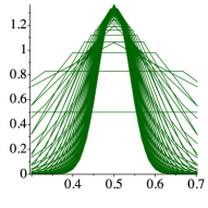
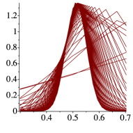
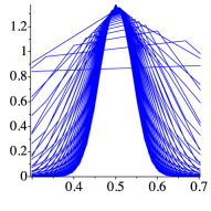
Type $B$ Eulerian	Lehmer’s $P_{n}$ (46)	Lehmer’s $R_{n}$ (47)
A060187 $\mathscr{A}(1,2,1)$	A185410 $\mathscr{A}(1,2,\frac{1}{2})$
$\bigl{(}{\frac{1}{2}n,\frac{1}{12}n+\frac{1}{12}}\bigr{)}$	$\bigl{(}{\frac{1}{2}n-\frac{1}{4},\frac{1}{12}n+\frac{1}{24}}\bigr{)}$	$\bigl{(}{\frac{1}{2}n-\frac{11}{12},\frac{1}{12}n-\frac{1}{360}}\bigr{)}$

Figure 3: While we have the same CLT $\mathscr{N}(\frac{1}{2}n,\frac{1}{12}n;n^{-\frac{1}{2}})$ for the three classes of polynomials, their differences are reflected in the finer asymptotic approximations to the mean and the variance, displayed in the last row with the format $($mean, variance$)$; see (39).

Stirling permutations of the second kind [175]: $\mathscr{A}(q,2,\frac{q}{2})$

Ma and Yeh [175] extended the Stirling permutations of Gessel and Stanley [112] and studied the so-called cycle ascent plateau, leading to polynomials of the type $\mathscr{A}(q,2,\frac{q}{2})$. When $q=1$, we get Lehmer’s polynomial (A185410), and when $q=2$, we get Eulerian numbers (up to a factor of $2^{n}$). The CLT $\mathscr{N}\bigl{(}{\frac{1}{2}n,\frac{1}{12}n;n^{-\frac{1}{2}}}\bigr{)}$ for the coefficients (for any real $q>0$) follows from Theorem 3.

Franssen’s $\mathscr{A}(p,2,p)$ [103]

The expansion

$$\left(\frac{u-v}{ue^{-(u-v)z}-ve^{(u-v)z}}\right)^{p}=\sum_{n\geqslant 0}R_{n}(u,v;p)\frac{z^{n}}{n!}$$

is studied in [103]. Let $P_{n}(v):=R_{n}(1,v;p)$. Then $P_{n}\in\mathscr{E}\langle\!\langle 2vn+p+(p-2)v,2v;1\rangle\!\rangle$, which is of type $\mathscr{A}(p,2,p)$. Note that when $p=1$ we get type $B$ Eulerian numbers and when $p=2$, we get $2^{n}\genfrac{<}{>}{0.0pt}{}{n+1}{k}$. For any real $p>0$, we then obtain the asymptotic normality $\mathscr{N}\bigl{(}{\frac{1}{2}n,\frac{1}{12}n;n^{-\frac{1}{2}}}\bigr{)}$ for the coefficients of $P_{n}$.

4.4 General $q>0$

Savage and Viswanathan’s $\mathscr{A}\bigl{(}{1,q,\tfrac{1}{q}}\bigr{)}$ [213]

A class of polynomials called $1/k$-Eulerian is examined in [213] (we changed their $k$ to $q$ for convenience) and is of type $P_{n}\in\mathscr{E}\langle\!\langle qvn+1-qv,qv;1\rangle\!\rangle$.

In addition to Eulerian numbers when $q=1$, one gets Lehmer’s polynomials (46) (or A185410) when $q=2$. By Corollary 4

$$X_{n}\bigl{(}{1,q,\tfrac{1}{q}}\bigr{)}\stackrel{{\scriptstyle d}}{{\thickapprox}}X_{n}\bigl{(}{0,1,\tfrac{1}{q}}\bigr{)}\stackrel{{\scriptstyle d}}{{\thickapprox}}X_{n}\bigl{(}{1,q,\tfrac{1}{q}+1}\bigr{)}\stackrel{{\scriptstyle d}}{{\thickapprox}}X_{n}\bigl{(}{q,q,\tfrac{1}{q}+1}\bigr{)},$$

for any $q>0$, which is a special case of (42) and (43).

Strasser’s $\mathscr{A}\bigl{(}{1,q,\tfrac{2}{q}}\bigr{)}$ [229]

A general framework studied in [229] is of the form $P_{n}\in\mathscr{E}\langle\!\langle qvn+1-(q-1)v,qv;1\rangle\!\rangle$, where $q=1,2,\dots$. These polynomials are palindromic. Note that when $q=0,1$ and $2$, one gets binomial coefficients A007318, Eulerian numbers A008292, and MacMahon numbers A060187, respectively.

A142458	$\mathscr{A}(1,3,\frac{2}{3})$	A142459	$\mathscr{A}(1,4,\frac{1}{2})$	A142460	$\mathscr{A}(1,5,\frac{2}{5})$
A142461	$\mathscr{A}(1,6,\frac{1}{3})$	A142462	$\mathscr{A}(1,7,\frac{2}{7})$	A167884	$\mathscr{A}(1,8,\frac{1}{4})$

On the other hand, the first few rows of $P_{n}(v)$ read $P_{1}(v)=1+v$, $P_{2}(v)=1+2(1+q)v+v^{2}$ and

$$P_{3}(v) =1+(3+6q+2q^{2})v+(3+6q+2q^{2})v^{2}+v^{3}.$$

Numerically,

$q$	$1$	$2$	$3$	$4$	$5$	$6$	$7$	$8$
$3+6q+2q^{2}$	$11$	$23$	$39$	$59$	$83$	$111$	$143$	$179$

We see that the CLT $\mathscr{N}\bigl{(}{\frac{1}{2}n,\frac{1}{12}n;n^{-\frac{1}{2}}}\bigr{)}$ remains the same for $q>0$ although these coefficients are more concentrated near the middle range for growing $q$.

Brenti’s $q$-Eulerian polynomials [25]

A different $q$-analogue of Eulerian numbers considered in [25] is of the form $P_{n}\in\mathscr{E}\langle\!\langle qvn+1-v,qv;1\rangle\!\rangle$, which is of type $\mathscr{A}(1,q,1)$; see also [226]. These polynomials also arise in the analysis of carries processes; see [193]. The reciprocal polynomials are of type $\mathscr{A}(q-1,q,1)$, which appeared on the webpage [166]. In addition to Eulerian and MacMahon numbers for $q=1$ and $q=2$, respectively, we also have

A225117	$\mathscr{A}(2,3,1)$	Reciprocal of $\mathscr{A}(1,3,1)$
A225118	$\mathscr{A}(3,4,1)$	Reciprocal of $\mathscr{A}(1,4,1)$
A158782	$\mathscr{A}(1,4,1)$	$v\mapsto v^{2}$: $\mathscr{E}\langle\!\langle 4v^{2}n+1-v^{2},2v(1+v);1\rangle\!\rangle$

The CLT and LLT when $q\geqslant 1$ were derived in [54] by the real-rootedness and Bender’s approach [14], respectively.

Eulerian numbers associated with arithmetic progressions

Eulerian numbers associated with the arithmetic progression $\{p,p+q,p+2q,\dots\}$ are considered in Xiong et al. [244], which corresponds to the polynomials $P_{n}\in\mathscr{E}\langle\!\langle qvn+(q-p)(1-v),qv(1-v);1\rangle\!\rangle$; see also [186, 205].

These polynomials are of type $\mathscr{A}(q-p,q,1)$, which have nonnegative coefficients when $0\leqslant p\leqslant q$.

By Corollary 4, $X_{n}(q-p,q,1)\stackrel{{\scriptstyle d}}{{\thickapprox}}X_{n}(p,q,1)$, and polynomials of the latter type arise in the following extension of Euler’s original construction

$$P_{n}(v):=(1-v)^{n+1}\sum_{j\geqslant 0}(p+qj)^{n}v^{j}\qquad(n\geqslant 1),$$

with $P_{0}(v)=1$ for a given pair $(p,q)$; see [87, 205]. The polynomials associated with the type $\mathscr{A}(p,q,1)$ were rediscovered in [211] in digital filters and those with $\mathscr{A}(q-p,q,1)$ in [201] in connection with sums of squares. In particular, $(p,q)=(1,0)$ or $(1,1)$ gives Eulerian numbers and $(p,q)=(1,2)$ the MacMahon numbers. Furthermore, two more sequences were found in OEIS:

A178640

$\mathscr{A}(5,8,1)=$ reciprocal of $\mathscr{A}(3,8,1)$

A257625

$\mathscr{A}(3,6,1)$

A more general type is studied in Barry [11]:

$$X_{n}(q(p+r)-p,q,p+r)\stackrel{{\scriptstyle d}}{{\thickapprox}}X_{n}(p,q,p+r);$$

Theorem 3 applies when $p\geqslant 0$, and $q,r>0$, and we get always the same CLT $\mathscr{N}\bigl{(}{\frac{1}{2}n,\frac{1}{12}n;n^{-\frac{1}{2}}}\bigr{)}$. See also [164] for other properties such as continued fraction expansions and $q$-log convexity.

Yet another type

$$X_{n}(qr-r+1,q,r)\stackrel{{\scriptstyle d}}{{\thickapprox}}X_{n}(r-1,q,r),$$

(referred to as the $r$-Eulerian-Fubini polynomials) was studied in [66]. The same CLT holds when $q>0$ and $r\geqslant 1$.

OEIS: $\mathscr{A}\bigl{(}{p,q,\tfrac{2p}{q}}\bigr{)}$

Two dozens of OEIS sequences have the pattern

$$[v^{k}]P_{n}(v)=\phi_{k}[v^{k}]P_{n-1}(v)+\phi_{n-k}[v^{k-1}]P_{n-1}(v)\qquad(1\leqslant k\leqslant n;n\geqslant 1),$$

with $P_{0}(v)=1$, where $\phi_{k}=p+qk$. Such polynomials $P_{n}$’s satisfy $P_{n}\in\mathscr{E}\langle\!\langle qvn+p+(p-q)v,qv;1\rangle\!\rangle$, which is of type $\mathscr{A}\bigl{(}{p,q,\tfrac{2p}{q}}\bigr{)}$. The sequences we found are listed below.

A256890	$\mathscr{A}(2,1,4)$	A257180	$\mathscr{A}(3,1,6)$	A257606	$\mathscr{A}(4,1,8)$
A257607	$\mathscr{A}(5,1,10)$	A257608	$\mathscr{A}(1,9,\frac{2}{9})$	A257609	$\mathscr{A}(2,2,2)$
A257610	$\mathscr{A}(2,3,\frac{4}{3})$	A257611	$\mathscr{A}(3,2,3)$	A257612	$\mathscr{A}(2,4,1)$
A257613	$\mathscr{A}(4,2,4)$	A257614	$\mathscr{A}(2,5,\frac{4}{5})$	A257615	$\mathscr{A}(5,2,5)$
A257616	$\mathscr{A}(2,6,\frac{2}{3})$	A257617	$\mathscr{A}(2,7,\frac{4}{7})$	A257618	$\mathscr{A}(2,8,\frac{1}{2})$
A257619	$\mathscr{A}(2,9,\frac{4}{9})$	A257620	$\mathscr{A}(3,3,2)$	A257621	$\mathscr{A}(3,4,\frac{3}{2})$
A257622	$\mathscr{A}(4,3,\frac{8}{3})$	A257623	$\mathscr{A}(3,5,\frac{6}{5})$	A257624	$\mathscr{A}(5,3,\frac{10}{3})$
A257625	$\mathscr{A}(3,6,1)$	A257626	$\mathscr{A}(6,3,4)$	A257627	$\mathscr{A}(3,7,\frac{6}{7})$

When $p=1$, one obtains Strasser’s generalizations and more OEIS sequences are listed above. Note that both $(1,1,2)$ and $(2,2,2)$ lead to Eulerian numbers and $(1,2,1)$ to MacMahon numbers. All these types of polynomials produce the same $\mathscr{N}\bigl{(}{\frac{1}{2}n,\frac{1}{12}n;n^{-\frac{1}{2}}}\bigr{)}$ limiting behavior.

A summarizing table for generic types

We summarize the above discussions in the following table, listing only generic types and their equivalent ones.

Table 6: A summary of generic types of $\mathscr{A}(p,q,r)$ and their equivalent ones.

References	Type & its equivalent types
LI Shanlan [160]	$\mathscr{A}(1,1,q+1);\mathscr{A}(q,1,q+1),\mathscr{A}(0,1,q),\mathscr{A}(q,1,q)$
Riordan [208] Foata and Schützenberger [101]	$\mathscr{A}(q,1,q);\mathscr{A}(0,1,q),\mathscr{A}(q,1,q+1),\mathscr{A}(1,1,q+1)$
Brenti [25], Luschny [166]	$\mathscr{A}(1,q,1);\mathscr{A}(q-1,1,1)$
Dwyer [82], Harris [124]	$\mathscr{A}(q,1,1);\mathscr{A}(1-q,1,1)$
Savage and Viswanathan [213]	$\mathscr{A}(1,q,\frac{1}{q});\mathscr{A}(0,1,\frac{1}{q}),\mathscr{A}(1,q,\frac{q+1}{q}),\mathscr{A}(q,q,\frac{q+1}{q})$
Strasser [229]	$\mathscr{A}(1,q,\frac{2}{q})$
Morisita [190] Carlitz and Scoville [37] Hitczenko and Janson [128]	$\mathscr{A}(p,1,p+q);\mathscr{A}(q,1,p+q)$
Xiong et al. [244], OEIS Eriksen et al. [87]	$\mathscr{A}(p,q,1);\mathscr{A}(q-p,q,1)$
Ma and Yeh [175]	$\mathscr{A}\bigl{(}{q,2,\frac{q}{2}}\bigr{)};\mathscr{A}\bigl{(}{0,2,\frac{q}{2}}\bigr{)},\mathscr{A}\bigl{(}{q,2,\frac{q+2}{2}}\bigr{)},\mathscr{A}\bigl{(}{2,2,\frac{q+2}{2}}\bigr{)}$
Franssens [103]	$\mathscr{A}(q,2,q)$
OEIS	$\mathscr{A}(p,q,\frac{2p}{q})$
Oden et al. [196]	$\mathscr{A}(p-q,q,\frac{2p}{q});\mathscr{A}(p+q,q,\frac{2p}{q})$
Corcino et al. [66]	$\mathscr{A}(pq-p+1,q,p);\mathscr{A}(p-1,q,p)$
Barry [11]	$\mathscr{A}(p,q,r);\mathscr{A}(qr-p,q,r)$

4.5 Other extensions with the same CLT and their variants

We briefly mention some other examples not of the form $\mathscr{A}(p,q,r)$ but with the same CLT $\mathscr{N}\bigl{(}{\frac{1}{2}n,\frac{1}{12}n}\bigr{)}$; more examples with the same CLT are discussed in Section 9.

4.5.1 The two examples in the Introduction

The first example (see Figure 2) is of the form $\mathscr{E}\langle\!\langle vn+(1+v)^{2},v;1\rangle\!\rangle$ with $\alpha(v)=\beta(v)=v$ and $\gamma(v)=(1+v)^{2}$. We can directly apply Theorem 1 and get the same CLT $\mathscr{N}\bigl{(}{\frac{1}{2}n,\frac{1}{12}n}\bigr{)}$ for the distribution of the coefficients. The EGF

$$e^{(1-v)z+v(1-e^{(1-v)z})}\left(\frac{1-v}{1-ve^{(1-v)z}}\right)^{5}$$

can be derived by the procedures in Section 3.1. Analytically, this is of the form $\mathscr{A}(1,1,5)$ times the entire function $e^{v(1-e^{(1-v)z})}$, and we get the optimal Berry-Esseen bound $n^{-\frac{1}{2}}$ by applying Theorem 2.

Similarly, the second example A244312 (7) in the Introduction leads to the same CLT $\mathscr{N}\bigl{(}{\frac{1}{2}n,\frac{1}{12}n}\bigr{)}$ by the method of moments because it can be rewritten as $P_{n}\in\mathscr{E}_{1}\langle\!\langle vn-1+(1-v)\mathbf{1}_{n\text{ is odd}},v;v\rangle\!\rangle$, where again $\alpha(v)=\beta(v)=v$, and $\gamma(v)$ is less important in the dominant terms of the asymptotic approximations to the moments. In particular, the mean and the variance are given respectively by

$$\mathbb{E}(X_{n})=\begin{cases}\frac{n^{2}}{2(n-1)},&n\geqslant 2\text{ is even };\\ \frac{n+1}{2},&n\geqslant 3\text{ is odd },\end{cases}\quad\text{and}\quad\mathbb{V}(X_{n})=\begin{cases}\frac{n(n^{2}-2n-2)}{12(n-1)^{2}},&n\geqslant 4\text{ is even};\\ \frac{(n+1)(n-3)}{12(n-2)},&n\geqslant 3\text{ is odd}.\end{cases}$$

The optimal Berry-Esseen bound is expected to be of order $n^{-\frac{1}{2}}$, but the analytic proof via Theorem 2 fails due to the lack of solution to the PDE (8) satisfied by the EGF of $P_{n}$. Note that it can be shown that

$$P_{n}(v)=(1-v)^{n}\sum_{j\geqslant 0}j^{\lfloor\frac{1}{2}n\rfloor}(j+1)^{\lceil\frac{1}{2}n\rceil-1}v^{j+1}\qquad(n\geqslant 1).$$

From this expression, we can derive the optimal Berry-Esseen bound $n^{-\frac{1}{2}}$; details will be given elsewhere.

In such a context, we see particularly that the method of moments provides more robustness in the variation of $\gamma(v)$ in the recurrence (9) as long as the coefficients $[v^{k}]P_{n}(v)$ remain nonnegative, although the analytic approach is not limited to Eulerian type or nonnegativity of the coefficients.

4.5.2 $r$-Eulerian numbers again

The following six OEIS sequences are all generated by the same recurrence $P_{n}\in\mathscr{E}_{2}\langle\!\langle vn+1,v\rangle\!\rangle$, with initial conditions $P_{2}(v)$ different from that ($1+4v+v^{2}$) of Eulerian numbers:

A166340	$1+8v+v^{2}$	A166341	$1+10v+v^{2}$	A166343	$1+12v+v^{2}$
A166344	$1+6v+v^{2}$	A166345	$1+2v+v^{2}$	A188587	$1+v+v^{2}$

See also the paper by Conger [63] for the polynomials $\mathscr{E}_{r}\langle\!\langle vn+1-2v,v;A_{r}(v)\rangle\!\rangle$ for fixed $r=1,2,\dots$, where $A_{r}(v)$ is Eulerian polynomial of order $r-1$. Since Theorem 1 does not depend specially on the initial conditions, we obtain the same CLT $\mathscr{N}\bigl{(}{\frac{1}{2}n,\frac{1}{12}n}\bigr{)}$ by a simple shift of the recurrence $n\mapsto n-r$ and then by applying Theorem 1. The corresponding EGF can also be worked out, which leads to an effective version of CLT by Theorem 2.

4.5.3 Eulerian numbers of type $D$

Brenti [25] (see also [51]) shows that the EGF of the Eulerian polynomials $P_{n}(v)$ of type $D$ is given by

$$F(z,v)=\frac{(1-v)\bigl{(}{e^{(1-v)z}-vze^{2(1-v)z}}\bigr{)}}{1-ve^{2(1-v)z}}.$$

By the decomposition ($P_{n}$ being palindromic)

$$F(z,v)-(1-v)z=\frac{1-v}{1-ve^{2(1-v)z}}\bigl{(}{e^{(1-v)z}-z}\bigr{)}\in\mathscr{A}(1,2,1)-z\mathscr{A}(0,2,1),$$

we see that, up to the term $(1-v)z$, type $D$ is a difference of type $B$ and type $A$ Eulerian numbers; see [227]. Theorem 1 does not apply because these polynomials do not have the pattern (9). However, the coefficients do satisfy the same CLT $\mathscr{N}\bigl{(}{\frac{1}{2}n,\frac{1}{12}n;n^{-\frac{1}{2}}}\bigr{)}$ by applying Theorem 2.

4.5.4 Exponential perturbation

Polynomials of the form

$$P_{n}(v)=(2vn+1-v)P_{n-1}(v)+2v(1-v)P_{n-1}^{\prime}(v)\mp v(1-v)^{n-1}\qquad(n\geqslant 1),$$

with $P_{0}(v)=0$ (for “$+$”) and $P_{0}(v)=1$ (for “$-$”) are studied in [20], which correspond to A262226 (“$-$”) and A262227 (“$+$”), respectively. The EGF equals

$$\frac{(1-v)e^{(1-v)z}}{2\bigl{(}{1-ve^{2(1-v)z}}\bigr{)}}\mp\frac{e^{(1-v)z}}{2}.$$

While Theorem 1 does not apply, the method of proof easily extends to this case because the extra “exponential perturbation” term does not contribute to the dominant asymptotics of all finite moments. We then get the same CLT $\mathscr{N}\bigl{(}{\frac{1}{2}n,\frac{1}{12}n}\bigr{)}$ (as that for $\mathscr{A}(1,2,1)$). For both polynomials, Theorem 2 applies.

Another sequence A180246 corresponds essentially to $\mathscr{A}(2,1,1)$ (differing by the term $(-v)^{n}$). This is a concrete polynomial with $p>qr$ (see (37) and (38)), and thus the coefficients are not all positive. More precisely, if $P_{n}$ is of type $\mathscr{A}(2,1,1)$, then $P_{n}$ is, up to minor exponential perturbation, of type $\mathscr{A}(0,1,1)$ (Eulerian numbers) because

$$e^{2(1-v)z}\frac{1-v}{1-ve^{(1-v)z}}=\frac{1}{v^{2}}\left(\frac{1-v}{1-ve^{(1-v)z}}+(1-v)\bigl{(}{1+ve^{(1-v)z}}\bigr{)}\right).$$

On the other hand, all coefficients $[v^{k}]P_{n}(v)$ are positive except the following three ones:

$$[z^{n}]P_{n}(v) =(-1)^{n},\quad[z^{n-1}]P_{n}(v)=(-1)^{n-1}(n+1),$$

$$[z^{n-2}]P_{n}(v) =(-1)^{n}\left(\binom{n+1}{2}+(-1)^{n}\right).$$

Thus if we consider the random variables defined via the absolute values of all coefficients, then we still obtain the same CLT $\mathscr{N}\bigl{(}{\frac{1}{2}n,\frac{1}{12}n;n^{-\frac{1}{2}}}\bigr{)}$ because the above possibly negative coefficients are asymptotically negligible. The same argument applies to the more general type $\mathscr{A}(p,1,1)$, or (see [124])

$$P_{n}(v)=\sum_{0\leqslant k\leqslant n}v^{k}\sum_{0\leqslant j\leqslant k}\binom{n+1}{j}(-1)^{j}(k+p-j)^{n},$$

where $p>1$. For,

$$e^{p(1-v)z}\frac{1-v}{1-ve^{(1-v)z}}=v^{-p}\frac{1-v}{1-ve^{(1-v)z}}+O(1),$$

uniformly for $z\sim-\frac{\log v}{1-v}$. Thus, up to a few possibly negative coefficients that are asymptotically negligible, the polynomials are essentially Eulerian polynomials.

Type $D$ Eulerian	A066094	$\mathscr{N}\bigl{(}{\frac{1}{2}n,\frac{1}{12}n;n^{-\frac{1}{2}}}\bigr{)}$
$\sum_{0\leqslant j\leqslant k}\binom{n+1}{j}(-1)^{j}(k+2-j)^{n}$	$|$A180246$|$	$\mathscr{N}\bigl{(}{\frac{1}{2}n,\frac{1}{12}n;n^{-\frac{1}{2}}}\bigr{)}$
Primary type $D$ Eulerian	A262226	$\mathscr{N}\bigl{(}{\frac{1}{2}n,\frac{1}{12}n;n^{-\frac{1}{2}}}\bigr{)}$
Complementary type $D$ Eulerian	A262227	$\mathscr{N}\bigl{(}{\frac{1}{2}n,\frac{1}{12}n;n^{-\frac{1}{2}}}\bigr{)}$

4.5.5 Eulerian polynomials multiplied by $1+v$

Let $P_{n}(v):=(1+v)\sum_{0\leqslant k<n}\genfrac{<}{>}{0.0pt}{}{n}{k}v^{k}$. Such polynomials arose in the study of low-dimensional lattices (see [65]), and satisfy the recurrence

$$\mathscr{E}\left\langle\!\left\langle vn+\frac{1-v}{1+v},v;1+v\right\rangle\!\right\rangle.$$

These polynomials correspond to A008518 and are specially interesting because $\gamma(v)$ (in the notation of Theorem 1) is not a polynomial. The same limit law $\mathscr{N}\bigl{(}{\frac{1}{2}n,\frac{1}{12}n}\bigr{)}$ holds by an extension of Theorem 1 (because $\gamma(v)=\frac{1-v}{1+v}$ is not analytic in $|v|\leqslant 1$). However, from the proof of Theorem 1, it is clear that the analyticity of $\gamma(v)$ in $|v|<1$ and the finiteness of $\gamma^{(j)}(1)$ for each $j\geqslant 0$ are sufficient to guarantee the same CLT. In contrast, Theorem 2 easily applies.

5 Applications II: $\alpha(v)\neq\beta(v)$ or quadratic $\alpha(v)$, $\beta(v)$

We consider in this section other Eulerian-type polynomials for which Theorem 1 applies. Exact solutions for the associated PDEs when $\alpha(v)\neq\beta(v)$ are still possible but they are often of a less explicit form (especially when compared with the equal case (37)). Yet our approaches still apply as far as the limit laws are concerned.

We discuss a few such frameworks for which explicit EGFs are available before specializing to concrete examples. Note that in all cases we discuss below, Theorem 1 applies and we obtain a CLT easily. Following the same spirit of Section 4, we use the special forms of EGFs for a more synthetic discussion of the examples as well as for establishing a stronger CLT with optimal rate by Theorem 2.

5.1 Polynomials with $(\alpha(v),\beta(v))=(qv,v)\Longrightarrow\mathscr{N}\bigl{(}{\frac{q}{q+1}\,n,\frac{q^{2}}{(q+1)^{2}(q+2)}\,n}\bigr{)}$

A class of higher-order Eulerian numbers is proposed in Barbero G. et al. [10] satisfying the recurrence $P_{n}\in\mathscr{E}\langle\!\langle qvn+p+(r-p-q)v,v;1\rangle\!\rangle$, where $q\geqslant 1$ and $r\geqslant p\geqslant 1$ are integers. The EGF has the closed-form expression [9]

$$F(z,v):=\sum_{n\geqslant 0}P_{n}(v)\frac{z^{n}}{n!}=\left(\frac{T_{q}\bigl{(}{e^{(1-v)^{q}z}S_{q}(v)}\bigr{)}}{v}\right)^{p}\left(\frac{1-v}{1-T_{q}\bigl{(}{e^{(1-v)^{q}z}S_{q}(v)}\bigr{)}}\right)^{r},$$ (48)

where $T_{q}(S_{q}(v))=S_{q}(T_{q}(v))=v$, $S_{q}$ is a one-parameter family of functions given by

$$S_{q}(v)=ve^{L_{q}(v)},\quad\text{with}\quad L_{q}(v)=\sum_{1\leqslant j<q}\binom{q-1}{j}\frac{(-v)^{j}}{j}.$$

If we change $L_{q}(v)$ to

$$L_{q}(v):=\int_{0}^{v}\frac{(1-t)^{q-1}-1}{t}\,\,\mathrm{d}{t},$$ (49)

then (48) holds for real $p,q,r$. For convenience, we write the framework (48) as $F\in\mathscr{T}(p,q.r)$.

Theorem 4.

Assume $P_{n}\in\mathscr{E}\langle\!\langle qvn+p+(r-p-q)v,v;1\rangle\!\rangle$. If

$$q\geqslant 1,r\geqslant p\geqslant 0,\text{ and }r+p>0,$$ (50)

then the coefficients of $P_{n}$ satisfy the CLT

$$\mathscr{N}\biggl{(}{\frac{q}{q+1}\,n,\frac{q^{2}}{(q+1)^{2}(q+2)}\,n;n^{-\frac{1}{2}}}\biggr{)}.$$ (51)

Proof.

By examining the corresponding recurrence for the coefficients, we see that if $q\geqslant 1$ and $r\geqslant p\geqslant 0$, then $[v^{k}]P_{n}(v)\geqslant 0$; the additional condition $r+p>0$ guarantees positivity of $P_{n}(1)$. Thus under (50), Theorem 1 applies and we see that the coefficients of $P_{n}(v)$ satisfy the CLT (51) without rate. On the other hand, Theorem 2 also applies by taking there $\kappa=r$ and

$$\Psi(z,v):=\frac{1-T_{q}\bigl{(}{e^{(1-v)^{q}z}S_{q}(v)}\bigr{)}}{1-v}.$$

The dominant singularity $\rho(v)$ is given by

$$\rho(v):=\frac{\log S_{q}(1)-\log S_{q}(v)}{(1-v)^{q}}=\frac{1}{(1-v)^{q}}\int_{v}^{1}t^{-1}(1-t)^{q-1}\,\mathrm{d}{t}.$$

The mean and the variance constants can then be computed by the relations $\rho^{\prime}(1)=-\frac{1}{q+1}$ and $\rho^{\prime\prime}(1)=\frac{2}{q+2}$. ∎

In particular,

$q=1$	$q=2$	$q=3$	$q=4$
$\mathscr{N}\bigl{(}{\frac{1}{2}n,\frac{1}{12}n}\bigr{)}$	$\mathscr{N}\bigl{(}{\frac{2}{3}n,\frac{1}{9}n}\bigr{)}$	$\mathscr{N}\bigl{(}{\frac{3}{4}n,\frac{9}{80}n}\bigr{)}$	$\mathscr{N}\bigl{(}{\frac{4}{5}n,\frac{8}{75}n}\bigr{)}$

Interestingly, as a function of $q$, the variance coefficient $\frac{q^{2}}{(q+1)^{2}(q+2)}$ first increases and then steadily decreases to $0$ as $q$ grows, the maximum occurring at $q=\frac{1+\sqrt{17}}{2}\approx 2.56$ with the value $\frac{1}{8}\bigl{(}{71-17\sqrt{17}}\bigr{)}\approx 0.113$.

The reciprocal polynomial of $P_{n}$ satisfies the recurrence

$$Q_{n}\in\mathscr{E}\langle\!\langle(q-1+v)n+r+1-p-q-(1-p)v,v;1\rangle\!\rangle,$$

whose coefficients follow the CLT $\mathscr{N}\bigl{(}{\frac{1}{q+1}\,n,\frac{q^{2}}{(q+1)^{2}(q+2)}\,n;n^{-\frac{1}{2}}}\bigr{)}$ under the same conditions $r\geqslant p\geqslant 0$, $r+p>0$ and $q\geqslant 1$.

5.1.1 $q=\frac{1}{2}\Longrightarrow\mathscr{N}\bigl{(}{\frac{1}{3}n,\frac{2}{45}n;n^{-\frac{1}{2}}}\bigr{)}$

David and Barton examined in their classical book [72] the number of increasing runs of length at least two (A008971), and the number of peaks in permutations (A008303), in addition to Eulerian numbers. They derived the corresponding recurrences:

# $(|\!\uparrow\!\!\text{ runs}|\geqslant 2)$ in permutations	A008971	$\mathscr{E}\langle\!\langle vn+1-v,2v;1\rangle\!\rangle$	$\mathscr{T}\bigl{(}{\frac{1}{2},\frac{1}{2},1}\bigr{)}$
# peaks in permutations	A008303	$\mathscr{E}_{1}\langle\!\langle vn+2(1-v),2v;1\rangle\!\rangle$	$\mathscr{T}\bigl{(}{1,\frac{1}{2},1}\bigr{)}$

The first few rows of both sequences are given in Table 7. To apply Theorem 4 (which starts the recurrence from $n=1$), we shift $n$ in both recurrences by $1$, changing $\gamma(v)$ from “$1-v$” and “$2(1-v)$” to “$1$” and “$2-v$” respectively. Then the polynomials $2^{-n}P_{n}(v)$ are of type $\mathscr{T}\bigl{(}{\frac{1}{2},\frac{1}{2},1}\bigr{)}$ and $\mathscr{T}\bigl{(}{1,\frac{1}{2},1}\bigr{)}$, respectively. We thus obtain the same CLT $\mathscr{N}\bigl{(}{\frac{1}{3}n,\frac{2}{45}n;n^{-\frac{1}{2}}}\bigr{)}$ for both statistics by Theorem 4. In particular, about two-thirds of runs have length $\geqslant 2$; also note that the variance constant $\frac{2}{45}$ is very small.

A008971
$n\backslash k$	$0$	$1$	$2$	$3$	$4$
$1$	$1$
$2$	$1$	$1$
$3$	$1$	$5$
$4$	$1$	$18$	$5$
$5$	$1$	$58$	$61$
$6$	$1$	$179$	$479$	$61$
$7$	$1$	$543$	$3111$	$1385$
$8$	$1$	$1636$	$18270$	$19028$	$1385$

A008303
$n\backslash k$	$0$	$1$	$2$	$3$
$1$	$1$
$2$	$2$
$3$	$4$	$2$
$4$	$8$	$16$
$5$	$16$	$88$	$16$
$6$	$32$	$416$	$272$
$7$	$64$	$1824$	$2880$	$272$
$8$	$128$	$7680$	$24576$	$7936$

Table 7: The first few rows of A008971 (left) and A008303 (right).

Instead of using (48), the exact solutions for the bivariate EGFs have the simpler alternative forms

$$\begin{split}\href https://oeis.org/A008971:\;&\frac{\sqrt{1-v}}{\sqrt{1-v}\cosh\bigl{(}{\sqrt{1-v}\,z}\bigr{)}-\sinh\bigl{(}{\sqrt{1-v}\,z}\bigr{)}},\\ \href https://oeis.org/A008303:\;&1+\frac{v\sinh\bigl{(}{\sqrt{1-v}\,z}\bigr{)}}{\sqrt{1-v}\cosh\bigl{(}{\sqrt{v-1}\,z}\bigr{)}-\sinh\bigl{(}{\sqrt{1-v}\,z}\bigr{)}},\end{split}$$ (52)

respectively, which can be derived directly by the approach of Section 3.1; see [53, 85, 169, 200, 238].

These numbers also appear in other different contexts [70, 121, 148, 181, 187, 195] (notably [148]). See also [97] for a connection to binary search trees. Désiré André [4] seems the first to give a detailed study of A008303 (up to a proper shift) where he examined the number of ascending or descending runs in cyclic permutations. He derived not only the recurrence for the polynomials and the first two moments of the distribution, but also solved the corresponding PDE for the EGF. For more information (including asymptotic normality), see [72, 238] and the references therein.

5.1.2 $q=1\Longrightarrow\mathscr{N}\bigl{(}{\frac{1}{2}n,\frac{1}{12}n;n^{-\frac{1}{2}}}\bigr{)}$

In this case, $L_{1}(z)=0$, $S_{1}(v)=T_{1}(v)=v$, so that

$$F(z,v)=e^{p(1-v)z}\left(\frac{1-v}{1-ve^{(1-v)z}}\right)^{r},$$

implying that $\mathscr{T}(p,1,r)=\mathscr{A}(p,1,r)$, which we already discussed in Section 4.

5.1.3 $q=2\Longrightarrow\mathscr{N}\bigl{(}{\frac{2}{3}n,\frac{1}{9}n;n^{-\frac{1}{2}}}\bigr{)}$

In this case, $S_{2}(z)=ze^{-z}$ and $T_{2}(z)=ze^{T_{2}(z)}=\sum_{n\geqslant 1}\frac{n^{n-1}}{n!}\,z^{n}$ is the Cayley tree function (essentially the Lambert $W$-function; see [67] and A000169), so that

$$F(z,v)=\left(\frac{T_{2}\bigl{(}{ve^{-v+(1-v)^{2}z}}\bigr{)}}{v}\right)^{p}\left(\frac{1-v}{1-T_{2}\bigl{(}{ve^{-v+(1-v)^{2}z}}\bigr{)}}\right)^{r}.$$ (53)

The simple relations

$$\partial_{z}\mathscr{T}(p,2,p)=p\mathscr{T}(p,2,p+2)\quad\text{and}\quad\partial_{z}\mathscr{T}(0,2,p)=pv\mathscr{T}(1,2,p+2),$$ (54)

imply an equivalence relation for the underlying random variables in each case.

In particular, $\mathscr{T}(0,2,1)$ gives the second order Eulerian numbers (or Eulerian numbers of the second kind): $P_{n}\in\mathscr{E}\langle\!\langle(2n-1)v,v;1\rangle\!\rangle$.

Such polynomials arise in many different combinatorial and computational contexts; see for example [29, 67, 110, 112, 120, 143, 156, 200] and OEIS A008517 for more information. In addition to enumerating the number of ascents in Stirling permutations (see [19, 112, 143]), we mention here two other relations: as derivative polynomials [67]

$$\mathbb{D}_{x}^{n+1}T_{2}(e^{x})=\frac{P_{n}(-T_{2}(e^{x}))}{(1-T_{2}(e^{x}))^{2n+1}}\qquad(n\geqslant 1),$$

and as coefficients in an asymptotic expansion [29]

$$\frac{n!}{(nv)^{n}}\left(e^{nv}-\sum_{0\leqslant j\leqslant n}\frac{(nv)^{j}}{j!}\right)=\sum_{0\leqslant j<K}\frac{(-1)^{j}P_{j}(v)}{n^{j}(1-v)^{2j+1}}+O\bigl{(}{n^{-K}}\bigr{)},$$

for any $K=1,2,\dots$.

The CLT $\mathscr{N}\bigl{(}{\frac{2}{3}n,\frac{1}{9}n}\bigr{)}$ seems first proved in [15, 180] in the context of leaves in plane-oriented recursive trees, and later in [19, 143], the approaches used including analytic, urn models and real-rootedness, respectively.

The corresponding reciprocal polynomials $Q_{n}(v):=v^{n+1}P_{n}(\frac{1}{v})$ satisfy $Q_{n}\in\mathscr{E}\langle\!\langle(1+v)n-1-2v,v;1\rangle\!\rangle$, which is A163936. We summarize these in the following table.

Second order Eulerian ($1\leqslant k\leqslant n$)	A008517	$\mathscr{T}(0,2,1)$	$\mathscr{N}\bigl{(}{\frac{2}{3}n,\frac{1}{9}n;n^{-\frac{1}{2}}}\bigr{)}$
Reciprocal of A008517	A112007		$\mathscr{N}\bigl{(}{\frac{1}{3}n,\frac{1}{9}n;n^{-\frac{1}{2}}}\bigr{)}$
Second order Eulerian ($0\leqslant k<n$)	A201637	$\mathscr{T}(1,2,1)$	$\mathscr{N}\bigl{(}{\frac{2}{3}n,\frac{1}{9}n;n^{-\frac{1}{2}}}\bigr{)}$
Reciprocal of A201637	A163936		$\mathscr{N}\bigl{(}{\frac{1}{3}n,\frac{1}{9}n;n^{-\frac{1}{2}}}\bigr{)}$
Essentially $=$ A163969	A288874		$\mathscr{N}\bigl{(}{\frac{1}{3}n,\frac{1}{9}n;n^{-\frac{1}{2}}}\bigr{)}$

In addition to $\mathscr{T}(0,2,1)$ and $\mathscr{T}(1,2,1)$, the polynomials defined on $\mathscr{T}(1,2,3)$ also correspond, by (54), to the second-order Eulerian numbers, and appeared in [89], together with two other variants:

$$\mathscr{T}(0,2,2)\text{ with }P_{0}(v)=v,\quad\text{and}\quad\mathscr{T}(1,2,0).$$

The first ($\mathscr{T}(0,2,2)$ and $\mathscr{T}(1,2,4)$ by (54)) leads, by Theorem 4, to the same $\mathscr{N}\bigl{(}{\frac{2}{3}n,\frac{1}{9}n;n^{-\frac{1}{2}}}\bigr{)}$ as for the second order Eulerian numbers because (50) holds. The second type ($\mathscr{T}(1,2,0)$) contains negative coefficients but corresponds essentially to the second order Eulerian numbers after dividing by $1-v$.

Another example with $q=2$ is sequence A214406, which is the second order Eulerian numbers of type $B$ and counts the Stirling permutations [112, 145] by ascents. The polynomials can be generated by $P_{n}\in\mathscr{E}\langle\!\langle 4vn+1-3v,2v;1\rangle\!\rangle$ and its reciprocal transform is $Q_{n}\in\mathscr{E}\langle\!\langle(2n-1)(1+v),2v;1\rangle\!\rangle$. By considering $2^{-n}P_{n}(v)$, we see that these numbers are of type $\mathscr{T}(\frac{1}{2},2,1)$ and the coefficients follow a CLT with optimal convergence rate.

The last example A290595 is of a different form: $P_{n}\in\mathscr{E}\langle\!\langle 3(1+v)n-2-v,3v;1\rangle\!\rangle$, whose reciprocal $Q_{n}$ satisfies $Q_{n}\in\mathscr{E}\langle\!\langle 6vn+2-5v,3v;1\rangle\!\rangle$ and is, up to the factor $3^{n}$, of type $\mathscr{T}\bigl{(}{\frac{2}{3},2,1}\bigr{)}$. Thus the EGF of $P_{n}$ is given by

$$\left(vT_{2}\bigl{(}{v^{-1}e^{-\frac{1}{v}(1-3(1-v)^{2}z)}}\bigr{)}\right)^{\frac{2}{3}}\left(\frac{v-1}{v\bigl{(}{1-T_{2}\bigl{(}{v^{-1}e^{-\frac{1}{v}(1-3(1-v)^{2}z)}}\bigr{)}}\bigr{)}}\right),$$

and we obtain the same CLT $\mathscr{N}\bigl{(}{\frac{1}{3}n,\frac{1}{9}n;n^{-\frac{1}{2}}}\bigr{)}$ for the distribution of $[v^{k}]P_{n}(v)$.

Second order Eulerian type $B$	A214406	$\mathscr{T}(\frac{1}{2},2,1)$	$\mathscr{N}\bigl{(}{\frac{2}{3}n,\frac{1}{9}n;n^{-\frac{1}{2}}}\bigr{)}$
Reciprocal of A214406	A288875		$\mathscr{N}\bigl{(}{\frac{1}{3}n,\frac{1}{9}n;n^{-\frac{1}{2}}}\bigr{)}$
$\mathscr{E}\langle\!\langle 6vn+2-5v,3v;1\rangle\!\rangle$		$\mathscr{T}(\frac{2}{3},2,1;3z)$	$\mathscr{N}\bigl{(}{\frac{2}{3}n,\frac{1}{9}n;n^{-\frac{1}{2}}}\bigr{)}$
Reciprocal of $\mathscr{T}\bigl{(}{\frac{2}{3},2,1;3z}\bigr{)}$	A290595		$\mathscr{N}\bigl{(}{\frac{1}{3}n,\frac{1}{9}n;n^{-\frac{1}{2}}}\bigr{)}$

See also Section 9.5 for polynomials related to $\mathscr{T}\bigl{(}{\frac{1}{q},2,1}\bigr{)}$.

5.1.4 $q=3\Longrightarrow\mathscr{N}\bigl{(}{\frac{3}{4}n,\frac{9}{80}n;n^{-\frac{1}{2}}}\bigr{)}$

We found only one OEIS example:

Third order Eulerian ($0\leqslant k<n$)

A219512

$\mathscr{T}(1,3,1)$

$\mathscr{N}\bigl{(}{\frac{3}{4}n,\frac{9}{80}n;n^{-\frac{1}{2}}}\bigr{)}$

or

$$P_{n}\in\mathscr{E}\langle\!\langle 3vn+1-3v,v;1\rangle\!\rangle.$$ (55)

For the EGF, in addition to Barbero G. et al.’s solution (48), an alternative form is as follows. Define $J(z,v)$

$$J(z,v):=\int_{0}^{z}\frac{\,\mathrm{d}{t}}{(1+t)(1+tv)^{3}}=\frac{\log\frac{w}{v}+2(v-w)-\tfrac{1}{2}(v^{2}-w^{2})}{(1-v)^{3}},$$

where $w:=\frac{v(1+z)}{1+vz}$. Then the EGF $F(z,v)-1$ is the compositional inverse of $J$, namely, it satisfies

$$F(J(z,v),v)-1=z.$$

This can be readily checked by (48). Indeed, for any polynomials of type $\mathscr{T}(1,q,1)$ with $q>0$, we have $F(J(z,v),v)-1=z$, where

$$J(z,v) :=\int_{0}^{z}\frac{\,\mathrm{d}{t}}{(1+t)(1+tz)^{q}}=\frac{1}{(1-v)^{q}}\left(\log\frac{1+z}{1+vz}+L_{q}\left(\frac{v(1+z)}{1+vz}\right)-L_{q}(v)\right),$$

with $L_{q}$ defined in (49).

Note that the random variables associated with the coefficients of $\mathscr{T}(1,3,1)$ are equivalent to those of $\mathscr{T}(1,3,4)$ by a simple shift $n\mapsto n+1$ in (55). We obtain the same CLT $\mathscr{N}\bigl{(}{\frac{3}{4}n,\frac{9}{80}n;n^{-\frac{1}{2}}}\bigr{)}$.

5.1.5 $q>1\Longrightarrow\mathscr{N}\bigl{(}{\frac{q}{q+1}\,n,\frac{q^{2}}{(q+1)^{2}(q+2)}\,n}\bigr{)}$

These higher order Eulerian numbers are discussed in [9, 10]; see also Section 9.6 on Pólya urn models. We list the CLTs for $q=4,\dots,7$; note that our results are not limited to integer $q$.

Type	CLT	Type	CLT
$\mathscr{E}\langle\!\langle 4vn+1-4v,v;1\rangle\!\rangle$	$\mathscr{N}\bigl{(}{\frac{4}{5}n,\frac{8}{75}n;n^{-\frac{1}{2}}}\bigr{)}$	$\mathscr{E}\langle\!\langle 5vn+1-5v,v;1\rangle\!\rangle$	$\mathscr{N}\bigl{(}{\frac{5}{6}n,\frac{25}{252}n;n^{-\frac{1}{2}}}\bigr{)}$
$\mathscr{E}\langle\!\langle 6vn+1-6v,v;1\rangle\!\rangle$	$\mathscr{N}\bigl{(}{\frac{6}{7}n,\frac{9}{98}n;n^{-\frac{1}{2}}}\bigr{)}$	$\mathscr{E}\langle\!\langle 7vn+1-7v,v;1\rangle\!\rangle$	$\mathscr{N}\bigl{(}{\frac{6}{7}n,\frac{49}{576}n;n^{-\frac{1}{2}}}\bigr{)}$

5.2 Polynomials with $(\alpha(v),\beta(v))=(p+qv,v)$
$\Longrightarrow$ $\mathscr{N}\bigl{(}{\frac{q}{p+q+1}\,n,\frac{q(p+1)(p+q)}{(p+q+1)^{2}(p+q+2)}\,n}\bigr{)}$

Rza̧dkowski and Urlińska [209] study the recurrence

$$P_{n}\in\mathscr{E}\langle\!\langle(p+qv)n+1-p-qv,v;1\rangle\!\rangle,$$ (56)

where $p,q$ are not necessarily integers. When $p=0$, we obtain higher order Eulerian numbers $\mathscr{T}(1,q,1)$; in particular, $(p,q)=(0,1)$ gives Eulerian numbers, and $(p,q)=(0,m)$ the $m$th order Eulerian numbers. If $[v^{k}]P_{n}(v)\geqslant 0$ for $n,k\geqslant 0$, then we obtain the CLT

$$\mathscr{N}(\mu n,\sigma^{2}n),\text{ where }\mu:=\frac{p}{p+q+1}\text{ and }\sigma^{2}:=\frac{q(p+1)(p+q)}{(p+q+1)^{2}(p+q+2)},$$ (57)

provided that the variance coefficient $\sigma^{2}>0$. Note that for fixed $q$ and increasing $p$, the mean coefficient $\mu$ increases to unity and the variance coefficient $\sigma^{2}$ first increases and then decreases to zero, while for fixed $p$ and increasing $q$, $\mu$ decreases steadily and $\sigma^{2}$ undergoes a similar unimodal pattern as in the case of fixed $q$ and increasing $p$.

By (32), we can also apply Theorem 2 by taking (assuming $p+q>0$)

$$\Psi(z,v)=\frac{1-T\bigl{(}{S(v)+\frac{(1-v)^{p+q}z}{v^{p}}}\bigr{)}}{1-v},\quad\text{where}\quad S(v)=\int_{v}^{1}t^{-p-1}(1-t)^{p+q-1}\,\mathrm{d}{t},$$

and $T(S(v))=v$. With the notations of Theorem 2, since

$$\rho(v)=\frac{v^{p}}{(1-v)^{p+q}}\int_{v}^{1}t^{-p-1}(1-t)^{p+q-1}\,\mathrm{d}{t},$$

we obtain $\rho^{\prime}(1)=-\frac{q}{(p+q)(p+q+1)}$ and $\rho^{\prime\prime}(1)=\frac{2q(q+1)}{(p+q)(p+q+1)(p+q+2)}$. We then deduce an optimal rate $n^{-\frac{1}{2}}$ in the CLT (57).

If $(p,q)=(-1,1)$, then $P_{n}(v)=v^{n-1}$. Another simple example for which $\sigma^{2}$ equals zero is $(p,q)=(-\frac{1}{2},\frac{1}{2})$ and in this case

$$P_{2n}(v)=\frac{v^{n-1}+v^{n}}{2},\quad\text{and}\quad P_{2n-1}(v)=v^{n},$$

which does not lead to a CLT.

Yet another example discussed in [209] is $(p,q)=(-\frac{1}{2},1)$ (which seems connected to A160468 in some way). We then obtain $\mathscr{N}\bigl{(}{\frac{2}{3}n,\frac{2}{45}n}\bigr{)}$ for the distributions of the coefficients. The EGF can be solved to be of the form

$$F(z,v)=\frac{1-v}{v}\cdot\frac{1+\sin\bigl{(}{\sqrt{v(1-v)}\,z+\arcsin(2v-1)}\bigr{)}}{1-\sin\bigl{(}{\sqrt{v(1-v)}\,z+\arcsin(2v-1)}\bigr{)}}.$$

To apply Theorem 2, we use the notation of (34) and take (due to a double zero)

$$\Psi(z,v)=\sqrt{\frac{1-\sin\bigl{(}{\sqrt{v(1-v)}z+\arcsin(2v-1)}\bigr{)}}{1-v}},$$

so that

$$\rho(v)=\frac{2\arccos\sqrt{v}}{\sqrt{v(1-v)}}=\frac{\pi-2\arcsin\sqrt{v}}{\sqrt{v(1-v)}}.$$

Thus Theorem 2 applies with $\rho^{\prime}(1)=-\frac{4}{3}$ and $\rho^{\prime\prime}(1)=\frac{32}{15}$, and we obtain the CLT with rate $\mathscr{N}\bigl{(}{\frac{2}{3}n,\frac{2}{45}n;n^{-\frac{1}{2}}}\bigr{)}$.

A CLT example with $\beta(1)<0$

An example reducible to the form $(\alpha(v),\beta(v))=(p+qv,v)$ but slightly different from (56) is Warren’s model of two-coin trials studied in [237], leading to the recurrence

$$P_{n}\in\mathscr{E}_{1}\langle\!\langle(1-\theta_{2}+\theta_{2}v)(n-1),-(\theta_{1}-\theta_{2})v;1-\theta_{2}+\theta_{2}v\rangle\!\rangle,$$

where $0<\theta_{1}\neq\theta_{2}<1$. Since $[v^{k}]P_{n}(v)\geqslant 0$ for all pairs $(\theta_{1},\theta_{2})$ by the original construction (or by examining the recurrence satisfied by the coefficients), we can apply Theorem 1 and obtain the CLT

$$\mathscr{N}\left(\frac{\theta_{2}}{1-\theta_{1}+\theta_{2}}\,n,\frac{(1-\theta_{1})\theta_{2}}{(1-2\theta_{1}+2\theta_{2})(1-\theta_{1}+\theta_{2})^{2}}\,n\right),$$

provided that $0<\theta_{1}<\theta_{2}+\frac{1}{2}$ (so that $1-2\theta_{1}+2\theta_{2}>0$). This example is interesting because if $\theta_{2}<\theta_{1}<\theta_{2}+\frac{1}{2}$, then, putting in the form of (9), we see that the factor

$$\beta(v)=-(\theta_{1}-\theta_{2})v$$

becomes negative at $v=1$, and this is one of the few examples in this paper with negative $\beta(1)$ and the coefficients of $P_{n}(v)$ still following a CLT. See Section 5.6 and [237] for other models of a similar nature. By solving the corresponding PDE (with $F(z,v)=(1-\theta_{2}+\theta_{2}v)z+O(z^{2})$ as $z\to 0$), we obtain the EGF

$$F(z,v) =\frac{1}{\theta_{2}-\theta_{1}}\log\frac{1-v}{1-T\bigl{(}{S(v)+v^{-\frac{1-\theta_{2}}{\theta_{2}-\theta_{1}}}(1-v)^{\frac{1}{\theta_{2}-\theta_{1}}}z}\bigr{)}}$$

$$\qquad+\frac{1-\theta_{2}}{\theta_{2}-\theta_{1}}\log\frac{T\bigl{(}{S(v)+v^{-\frac{1-\theta_{2}}{\theta_{2}-\theta_{1}}}(1-v)^{\frac{1}{\theta_{2}-\theta_{1}}}z}\bigr{)}}{v},$$

where $T(S(v))=v$ and

$$S(v):=\frac{1}{\theta_{2}-\theta_{1}}\int v^{-\frac{1-\theta_{2}}{\theta_{2}-\theta_{1}}-1}(1-v)^{\frac{1}{\theta_{2}-\theta_{1}}-1}\,\mathrm{d}{v}.$$

Another extension studied in [44] has the form $P_{n}\in\mathscr{E}\langle\!\langle n+h_{n}(v-1),v;1\rangle\!\rangle$ for some given sequence $h_{n}$. In the case when $h_{n}=p+qn$, we obtain the CLT

$$\mathscr{N}\biggl{(}{\frac{q}{2}\,n,\frac{q(2-q)}{12}\,n}\biggr{)},$$

by Theorem 1 when the coefficients are nonnegative and $0<q<2$.

5.3 Polynomials with $(\alpha(v),\beta(v))=\bigl{(}{\frac{1}{2}(1+v),\frac{1}{2}(3+v)}\bigr{)}\Longrightarrow\mathscr{N}\bigl{(}{\frac{1}{6}n,\frac{23}{180}n}\bigr{)}$

The sequence A162976 counts the number of permutations of $n$ elements having exactly $k$ double and initial descents; the generating polynomials $P_{n}$ satisfy the recurrence $P_{n}\in\mathscr{E}_{1}\langle\!\langle\tfrac{1}{2}(1+v)n,\tfrac{1}{2}(3+v);1\rangle\!\rangle$. This recurrence can be verified by the EGF

$$F(z,v)=1-\frac{2}{1+v-\sqrt{(1-v)(3+v)}\,\cot\bigl{(}{\frac{1}{2}z\sqrt{(1-v)(3+v)}}\bigr{)}},$$ (58)

obtained by using the expression in Goulden and Jackson’s book [119, p. 195, Ex. 3.3.46] after a direct simplification; see also Zhuang [247]. The CLT $\mathscr{N}\bigl{(}{\frac{1}{6}n,\frac{23}{180}n}\bigr{)}$ for the coefficients of $P_{n}$ follows easily from Theorem 1. Theorem 2 also applies with the dominant singularity at

$$\rho(v)=\frac{2\arccos\frac{1+v}{2}}{\sqrt{(1-v)(3+v)}}.$$ (59)

Two other recurrences arise from a study of similar permutation statistics in [247]:

$$P_{n}(v) =\frac{(1+v)n\pm(1-v)}{2}\,P_{n-1}(v)+\frac{(3+v)(1-v)}{2}\,P_{n-1}^{\prime}(v)\pm\frac{(1-v)(n-1)}{2}\,P_{n-2}(v),$$ (60)

for $n\geqslant 2$ with $P_{0}(v)=1$. These recurrences follow from the EGFs ($w:=\sqrt{(1-v)(3+v)}$)

$$\frac{w\,e^{\pm\frac{1}{2}(1-v)z}}{w\cos\bigl{(}{\frac{1}{2}zw}\bigr{)}-(1+v)\sin\bigl{(}{\frac{1}{2}zw}\bigr{)}},$$ (61)

derived in [247]; see also [84]. Taking both plus signs on the right-hand side of (60) together with $P_{1}(v)=1$ gives the sequence A162975 (enumerating double ascents); the other recurrence with both minus signs together with $P_{1}(v)=v$ gives the sequence A097898 (enumerating left-right double ascents or unit-length runs); see [113, 247] for more information. Theorem 1 does not apply directly but the same method of moments do and we get the same CLT $\mathscr{N}\bigl{(}{\frac{1}{6}n,\frac{23}{180}n}\bigr{)}$. The main reason that the method of moments works for (60) is that the last term is asymptotically negligible after the normalization $\bar{P}_{n}(v):=\frac{P_{n}(v)}{P_{n}(1)}=\frac{P_{n}(v)}{n!}$:

$$\bar{P}_{n}(v)=\frac{(1+v)n\pm(1-v)}{2n}\,\bar{P}_{n-1}(v)+\frac{(3+v)(1-v)}{2n}\,\bar{P}_{n-1}^{\prime}(v)\pm\frac{1-v}{2n}\,\bar{P}_{n-2}(v).$$

Alternatively, one applies the analytic method to the EGFs (61) (with the same $\rho(v)$ as (59)) and obtains additionally an optimal convergence rate in the CLT $\mathscr{N}\bigl{(}{\frac{1}{6}n,\frac{23}{180}n;n^{-\frac{1}{2}}}\bigr{)}$.

OEIS	coeff. $P_{n-1}(v)$	ceoff. $P_{n-1}^{\prime}(v)$	coeff. $P_{n-2}(v)$	$(\mu_{n},\sigma_{n}^{2})$
A162976	$\frac{(1+v)n}{2}$	$\frac{(3+v)(1-v)}{2}$	$0$	$\bigl{(}{\frac{1}{6}n+\frac{1}{6},\frac{23}{180}n+\frac{23}{180}}\bigr{)}$
A162975	$\frac{(1+v)n+1-v}{2}$	$\frac{(3+v)(1-v)}{2}$	$\frac{(n-1)(1-v)}{2}$	$\bigl{(}{\frac{1}{6}n-\frac{1}{3},\frac{23}{180}n-\frac{37}{180}}\bigr{)}$
A097898	$\frac{(1+v)n-1+v}{2}$	$\frac{(3+v)(1-v)}{2}$	$-\frac{(n-1)(1-v)}{2}$	$\bigl{(}{\frac{1}{6}n+\frac{2}{3},\frac{23}{180}n+\frac{83}{180}}\bigr{)}$

We also show in this table the differences in the lower order terms of the asymptotic mean and asymptotic variance.

5.4 Polynomials with quadratic $\alpha(v)$

We consider in this subsection recurrences of the form (9) where $\alpha(v)$ is a quadratic polynomial.

5.4.1 $(\alpha(v),\beta(v))=(v^{2},v(1+v))\Longrightarrow\mathscr{N}\bigl{(}{\tfrac{2}{3}n,\tfrac{8}{45}n}\bigr{)}$

Most of the examples we found involving quadratic $\alpha(v)$ have the form (after a shift of $n$ or a change of scales) $P_{n}\in\mathscr{E}\langle\!\langle v^{2}n+q-p+pv-v^{2},v(1+v);1\rangle\!\rangle$. For such a pattern, since the degree of $P_{n}$ is $n$, it proves simpler to look at its reciprocal $Q_{n}(v)=v^{n}P_{n}(\frac{1}{v})$, which then has the simpler generic form $Q_{n}\in\mathscr{E}\langle\!\langle vn+p+(q-p-1)v,1+v;1\rangle\!\rangle$. If $q\geqslant p>0$, then $[v^{k}]P_{n}(v)\geqslant 0$ and $P_{n}(1)>0$, and we obtain, by Theorem 1, the CLTs $\mathscr{N}\bigl{(}{\tfrac{1}{3}n,\tfrac{8}{45}n}\bigr{)}$ and $\mathscr{N}\bigl{(}{\tfrac{2}{3}n,\tfrac{8}{45}n}\bigr{)}$ for the coefficients of $Q_{n}$ and of $P_{n}$, respectively.

We now show how to enhance the CLTs by computing the corresponding EGFs. In general, assume $Q_{n}\in\mathscr{E}\langle\!\langle vn+p+(q-p-1)v,1+v\rangle\!\rangle$. Let $G(z,v)$ be the EGF of $Q_{n}(v)$. Then $G$ satisfies the PDE

$$(1-vz)\partial_{z}G-(1-v^{2})\partial_{v}G=(p+(q-p)v)G,$$

with $G(0,v)=Q_{0}(v)$. The solution, by the method of characteristics described in Section 3.1, is given by ($u:=\sqrt{1-v^{2}}$ and $w=\arcsin(v)$)

$$\begin{split}G(z,v)&=Q_{0}\bigl{(}{\sin(uz+w)}\bigr{)}\left(\frac{1+\sin(uz+w)}{1+v}\right)^{p}\left(\frac{u}{\cos(uz+w)}\right)^{q}.\end{split}$$ (62)

Write this class of functions as $\mathscr{Q}(p,q)$. Then

$$\partial_{z}\mathscr{Q}(q,q)=q\mathscr{Q}(q,q+1)\quad\text{when}\quad Q_{0}(v)=1.$$ (63)

With (62) available, we can apply Theorem 2 when $q\geqslant p>0$ with $\rho(v)=\frac{\arccos(v)}{\sqrt{1-v^{2}}}$, and the local expansion

$$-\log\rho(e^{s})=\tfrac{1}{3}s+\tfrac{4}{45}s^{2}+\tfrac{8}{2835}s^{3}-\tfrac{44}{14175}s^{4}+\cdots,$$

giving the CLT with optimal rate $\mathscr{N}\bigl{(}{\frac{1}{3}n,\frac{8}{45}n;n^{-\frac{1}{2}}}\bigr{)}$.

Liagre’s $\mathscr{Q}(2,3)$ and $\mathscr{Q}(1,3)$

Jean-Baptiste Liagre [161] studied (motivated by a statistical problem) as early as 1855 the combinatorial and statistical properties of the number of turning points (peaks and valleys) in permutations, and as far as we were aware, his paper [161] is the first publication on permutation statistics leading to an Eulerian recurrence, and contains the two recurrences

$$\begin{cases}P_{n}\in\mathscr{E}_{2}\langle\!\langle v^{2}n+1+2v-3v^{2},v(1+v);1\rangle\!\rangle,\\ P_{n}\in\mathscr{E}_{3}\langle\!\langle v^{2}n+1+v-3v^{2},v(1+v);1\rangle\!\rangle.\end{cases}$$ (64)

The former (A008970) counts the number of turning points in permutations of $n$ elements divided by two, while the latter (not in OEIS) that in cyclic permutations divided by two.

We can apply Theorem 1 by a direct shift of the two recurrences (so both has the initial conditions $P_{0}(v)=1$), and obtain the same CLT $\mathscr{N}\bigl{(}{\frac{2}{3}n,\frac{8}{45}n}\bigr{)}$. The CLT for A008970 can be obtained by the general theorem of Wolfowitz in [241] although, quite unexpectedly, it was first stated (without proof) by Bienaymé as early as 1874 in a very short note [16] (with a total of 13 lines); see also Netto’s book [194, pp. 105–116]. Bienaymé’s result is described as “far ahead of its time” in Heyde and Seneta’s book [127]. For more historical accounts, see [12, 127, 238]. The normalized versions (with $P_{0}(v)=1$) are given as follows.

$\frac{1}{2}\#$($n$-perms. with $k$ turning points)	A008970	$\mathscr{E}\langle\!\langle v^{2}n+1+2v-v^{2},v(1+v);1\rangle\!\rangle$
$\frac{1}{2}\#$($n$-cyclic perms. with $k$ turning points)		$\mathscr{E}\langle\!\langle v^{2}n+1+v,v(1+v);1\rangle\!\rangle$

The reciprocal polynomials $Q_{n}(v):=v^{n-2}P_{n-2}\bigl{(}{\frac{1}{v}}\bigr{)}$ and $Q_{n}(v):=v^{n-2}P_{n-3}\bigl{(}{\frac{1}{v}}\bigr{)}$ are of type $\mathscr{Q}(2,3)$ and $\mathscr{Q}(1,3)$, respectively, with the initial condition $Q_{0}(v)=1$ and $Q_{0}(v)=v$, respectively. By (62), we have the EGFs of $P_{n}$ and $Q_{n}$, respectively ($u:=\sqrt{1-v^{2}}$ and $w=\arcsin(v)$):

$$\begin{cases}\left(\dfrac{1+\sin(uz+w)}{1+v}\right)^{2}\left(\dfrac{u}{\cos(uz+w)}\right)^{3},\\ \sin(uz+w)\dfrac{(1+\sin(uz+w)}{1+v}\left(\dfrac{u}{\cos(uz+w)}\right)^{3}.\end{cases}$$

Note that in the first case, an alternative form for the EGF was derived by Morley [191] in 1897

$$\sum_{n\geqslant 1}\frac{Q_{n+1}(v)}{n!}\,z^{n}=\frac{1-v}{(1+v)\bigl{(}{1-\sin\bigl{(}{uz+w}\bigr{)}}\bigr{)}}-\frac{1}{1+v},$$

which can be obtained by a direct integration of $\mathscr{Q}(2,3)$. These EGFs are then suitable for applying Theorem 2, and an optimal Berry-Esseen bound is thus implied in the corresponding CLTs for the coefficients.

Alternating runs in permutations: $\mathscr{Q}(2,2)$

By (63), we see that the total number of turning points or alternating runs (which is twice A008970) in all permutations of $n$ elements (not half of them) is of type $\mathscr{Q}(2,2)$. This corresponds to sequence A059427. For more details and information, see David and Barton’s book [72, pp. 158–161], the review paper [12] and [3, 17, 18]. The normalized version (with $P_{0}(v)=1$) is

alternating runs in perms.

A059427

$\mathscr{E}\langle\!\langle v^{2}n+2v-v^{2},v(1+v);1\rangle\!\rangle$

$\mathscr{N}\bigl{(}{\frac{1}{3}n,\frac{8}{45}n;n^{-\frac{1}{2}}}\bigr{)}$

This sequence of polynomials has a larger literature than Liagre’s statistics. In particular, finding closed-form expressions for $[v^{k}]P_{n}(v)$ has been the subject of many papers; see for example [168, 169] and the references therein.

Alternating runs in up signed permutations: $\mathscr{Q}\bigl{(}{\frac{3}{2},2}\bigr{)}$

Extending further the alternating runs to signed permutations, Chow and Ma [52] studied the recurrence

$$P_{n}\in\mathscr{E}_{1}\langle\!\langle 2v^{2}n-1+3v-2v^{2},2v(1+v);v\rangle\!\rangle.$$ (65)

They also derived the closed form expression for the EGF of $P_{n}$:

$$\frac{1}{1+v}+\frac{v\sqrt{1-v}}{(1+v)\sqrt{\cosh\bigl{(}{2z\sqrt{1-v^{2}}}\bigr{)}-v-\sqrt{1-v^{2}}\sinh\bigl{(}{2z\sqrt{1-v^{2}}}\bigr{)}}}.$$

The reciprocal transformation $Q_{n}=v^{n}P_{n}\bigl{(}{\frac{1}{v}}\bigr{)}$ satisfies

$$Q_{n}\in\mathscr{E}_{1}\langle\!\langle 2vn+3(1-v),2(1+v);1\rangle\!\rangle.$$

This is of type $\mathscr{Q}\bigl{(}{\frac{3}{2},2}\bigr{)}$ after normalizing $Q_{n}(v)$ by $2^{n}$. Thus the same CLT $\mathscr{N}\bigl{(}{\frac{2}{3}n,\frac{8}{45}n;n^{-\frac{1}{2}}}\bigr{)}$ holds for the distribution of the number of alternating runs in signed permutations.

Derivative polynomials: $\mathscr{Q}(0,2)$

Another sequence A198895, which corresponds to the derivative polynomials of $\tan v+\sec v$, satisfies the recurrence

$$P_{n}\in\mathscr{E}_{1}\langle\!\langle v^{2}n+1-v^{2},v(1+v);1+v\rangle\!\rangle.$$

One gets the CLT$\bigl{(}{\frac{2}{3}n,\frac{8}{45}n;n^{-\frac{1}{2}}}\bigr{)}$ for the coefficients $[v^{k}]P_{n}(v)$, a result (without rate) also proved in [167] by the real-rootedness approach. Its reciprocal polynomial satisfies the simpler form

$$Q_{n}\in\mathscr{E}\langle\!\langle vn,1+v;1+v\rangle\!\rangle.$$

This is of type $\mathscr{Q}(0,2)$.

Up-down runs in permutations: $\mathscr{Q}(1,2)$

A very similar sequence is A186370 (number of permutations of $n$ elements having $k$ up-down runs):

$$P_{n}\in\mathscr{E}_{1}\langle\!\langle v^{2}n+v-v^{2},v(1+v);v\rangle\!\rangle.$$

One gets the same CLT $\mathscr{N}\bigl{(}{\frac{2}{3}n,\frac{8}{45}n;n^{-\frac{1}{2}}}\bigr{)}$. Its reciprocal polynomial satisfies the simpler form

$$Q_{n}\in\mathscr{E}_{1}\langle\!\langle vn+1-v,1+v;1\rangle\!\rangle,$$

which is of type $\mathscr{Q}(1,2)$. Interestingly, $Q_{1}(v)=v$ generates the same sequence of polynomials for $n\geqslant 2$.

5.4.2 $(\alpha(v),\beta(v))=\bigl{(}{\frac{1}{2}(1+v^{2}),\frac{1}{2}(1+v^{2})}\bigr{)}\Longrightarrow\mathscr{N}\bigl{(}{\frac{1}{2}n,\frac{5}{12}n}\bigr{)}$

The generating polynomials for the numbers of alternating descents ($\pi(i)\gtrless\pi(i+1)$ depending on the parity of $i$) or for the number of $3$-descents (either of the patterns $132$, $213$ or $321$) satisfy (see [47, 174])

$$P_{n}\in\mathscr{E}_{1}\langle\!\langle\tfrac{1}{2}(1+v^{2})n+v(1-v),\tfrac{1}{2}(1+v^{2});1\rangle\!\rangle.$$

They are palindromic and correspond to A145876.

This leads, by Theorem 1, to the CLT $\mathscr{N}\bigl{(}{\frac{1}{2}n,\frac{5}{12}n}\bigr{)}$ for the coefficients. For the optimal convergence rate $n^{-\frac{1}{2}}$, we can use the EGF derived in [47] (see also [247])

$$\frac{1+\sin((1-v)z)-\cos((1-v)z)}{\cos((1-v)z)-v-v\sin((1-v)z)},$$ (66)

and then apply Theorem 2 with

$$\rho(v)=\frac{\text{arccos}\bigl{(}{\frac{2v}{1+v^{2}}}\bigr{)}}{v-1}.$$

A very interesting property of $P_{n}(v)$ is that all roots lie on the left half unit circle, namely, $v=e^{i\theta}$ with $\frac{1}{2}\pi\leqslant\theta\leqslant\frac{3}{2}\pi$; see [174] for more information and Figure 4 for an illustration. Such a root-unitary property implies an alternative proof of the CLT via the fourth moment theorem of [138]: the fourth centered and normalized moment tends to three iff the coefficients are asymptotically normally distributed. This is in contrast to proving the unboundedness of the variance when all roots are real; also without the root-unitary property Theorem 1 requires the moments of all orders.

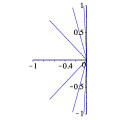
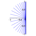
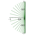
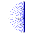
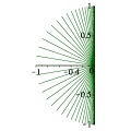
Figure 4: Distribution of the zeros of the A145876 polynomials $P_{n}(v)$ for $n=10,20,\dots,60$.

5.4.3 $(\alpha(v),\beta(v))=(v(1+v),v(1+v))\Longrightarrow\mathscr{N}\bigl{(}{\frac{3}{4}n,\frac{7}{48}n}\bigr{)}$

In the context of tree-like tableaux, the generating polynomial for the number of symmetric tree-like tableaux of size $2n+1$ with $k$ diagonal cells satisfies the recurrence [7]

$$P_{n}\in\mathscr{E}\langle\!\langle v(1+v)n,v(1+v);v\rangle\!\rangle.$$ (67)

We obtain, by Theorem 1, the CLT $\mathscr{N}\bigl{(}{\frac{3}{4}n,\frac{7}{48}n}\bigr{)}$ for the coefficients. This CLT was proved in [130] by the real-rootedness approach. The reciprocal polynomial $Q_{n}(v)=v^{n+1}P_{n}\bigl{(}{\frac{1}{v}}\bigr{)}$ satisfies the simpler recurrence $Q_{n}\in\mathscr{E}\langle\!\langle(1+v)n,1+v;1\rangle\!\rangle$, where the right-hand side differs from that of $P_{n}$ only by a factor $v$. By the techniques of Section 3.1, the EGF has the exact form

$$F(z,v)=\frac{v(1-v)}{(1+v)e^{z(v-1)}-2v}=e^{(1-v)z}\frac{v(1-v)}{1+v-2ve^{(1-v)z}},$$ (68)

which can then be used to prove an optimal Berry-Esseen bound $\mathscr{N}\bigl{(}{\frac{3}{4}n,\frac{7}{48}n;n^{-\frac{1}{2}}}\bigr{)}$ by Theorem 2 with $\rho(v)=\frac{1}{1-v}\log\frac{1+v}{2v}$.

See also [6] for another recurrence of the same type $P_{n}\in\mathscr{E}\langle\!\langle v(1+v)n+1+v-v^{2},v(1+v)\rangle\!\rangle$ whose reciprocal is of type $\mathscr{E}\langle\!\langle(1+v)n+1,1+v\rangle\!\rangle$. We have the same CLT for the coefficients.

5.4.4 $(\alpha(v),\beta(v))=(2v^{2},v(1+v))\Longrightarrow\mathscr{N}\bigl{(}{n,\frac{1}{3}n}\bigr{)}$

The $n$th order $\theta$-derivative $\theta:=v\mathbb{D}_{v}$ of $\sqrt{\frac{1+v}{1-v}}$ leads to the sequence of polynomials [173]

$$P_{n}\in\mathscr{E}\langle\!\langle v(2vn+1-2v),v(1+v);1\rangle\!\rangle;$$ (69)

these polynomials are palindromic and correspond to A256978. The degree of $P_{n}$ is $2n-1$, and the CLT $\mathscr{N}\bigl{(}{n,\frac{1}{3}n}\bigr{)}$ follows from Theorem 1. Furthermore, since the EGF of $P_{n}$ satisfies [173]

$$\sqrt{\frac{(1-v)\bigl{(}{1+ve^{(1-v^{2})z}}\bigr{)}}{(1+v)\bigl{(}{1-ve^{(1-v^{2})z}}\bigr{)}}},$$ (70)

we obtain additionally the stronger CLT $\mathscr{N}\bigl{(}{n,\frac{1}{3}n;n^{-\frac{1}{2}}}\bigr{)}$ by Theorem 2 with $\rho(v)=-\frac{\log v}{1-v^{2}}$.

More generally, the same CLT holds for the $\theta$-derivative polynomials of $\bigl{(}{\frac{1+v}{1-v}}\bigr{)}^{q}$ (with $q>0$) satisfying $P_{n}\in\mathscr{E}\langle\!\langle 2v((n-1)v+q),v(1+v);1\rangle\!\rangle$. Note that the usual derivative polynomial of $\sqrt{\frac{1+v}{1-v}}$ leads to polynomials of the type $P_{n}\in\mathscr{E}\langle\!\langle 2vn+1-2v,1+v;1\rangle\!\rangle$ with a different CLT; see Section 5.5.1.

Another example of the form $P_{n}\in\mathscr{E}\langle\!\langle 2v^{2}n+1+v,v(1+v);1+v\rangle\!\rangle$ appeared in [38], which enumerates the rises (or falls) in permutations of $2n$ elements satisfying $2n+1-\pi(j)=\pi(2n+1-j)$; see [2, 171] for a shifted version of the form $P_{n}\in\mathscr{E}\langle\!\langle 2v^{2}n+1+v-2v^{2},v(1+v);1\rangle\!\rangle$ (enumerating the flag-descent statistic in signed permutations). The CLT $\mathscr{N}\bigl{(}{n,\frac{1}{3}n}\bigr{)}$ for the coefficients of both polynomials holds by Theorem 1. Note that the latter $P_{n}$ (from [2]) corresponds to A101842 and can be computed by

$$P_{n}(v)=(1+v)^{n}\sum_{0\leqslant k<n}\genfrac{<}{>}{0.0pt}{}{n}{k}v^{k},$$

implying that the EGF is given by

$$e^{(1-v^{2})z}\frac{1-v}{1-ve^{(1-v^{2})z}}.$$

Then Theorem 2 applies with $\rho(v)=\frac{-\log v}{1-v^{2}}$ and an optimal convergence rate $n^{-\frac{1}{2}}$ in the CLT is guaranteed; see Figure 5 for the histograms and finer expressions of the mean and the variance.

More generally, all polynomials $P_{n}$ of the form $(1+v)^{n}R_{n}(v)$, where $R_{n}(v)$ is of type $\mathscr{A}(p,q,r)$ with $p,q,r\geqslant 0$ and $qr\geqslant p\geqslant 0$, are Eulerian with $(\alpha(v),\beta(v))=(2qv^{2},qv(1+v))$, which leads to the same CLT $\mathscr{N}\bigl{(}{n,\frac{1}{3}n;n^{-\frac{1}{2}}}\bigr{)}$. An OEIS instance of this type is A165891, which corresponds to $\mathscr{E}\langle\!\langle 2v^{2}n+1+2v-v^{2},v(1+v);1\rangle\!\rangle$ and is related to A101842 by a factor of $1+v$; see Figure 5.

OEIS	A256978	A101842	A165891
$a_{n}(v)$	$2v^{2}n+v-2v^{2}$	$2v^{2}n+1+v-2v^{2}$	$2v^{2}n+1+2v-v^{2}$
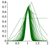
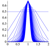
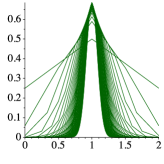
$(\mathbb{E}(X_{n}),\mathbb{V}(X_{n})))$	$\bigl{(}{n,\frac{n(n-1)(4n-5)}{3(2n-1)(2n-3)}}\bigr{)}$	$\bigl{(}{n-\frac{1}{2},\frac{1}{3}n+\frac{1}{12}}\bigr{)}$	$\bigl{(}{n,\frac{1}{3}n+\frac{1}{6}}\bigr{)}$

Figure 5: The histograms of the three OEIS polynomials of the format $\mathscr{E}\langle\!\langle a_{n}(v),v(1+v);1\rangle\!\rangle$ for $n=2,\dots,50$. Their coefficients all satisfy the same CLT $\mathscr{N}(n,\frac{1}{3}n;n^{-\frac{1}{2}})$ and their differences in the exact mean and the exact variance are shown in the last row.

5.5 Polynomials with an extra normalizing factor

We discuss in this subsection polynomials of the form

$$R_{n}\in\mathscr{E}\left\langle\!\left\langle\frac{\alpha(v)n+\gamma(v)}{e_{n}},\frac{\beta(v)}{e_{n}}\right\rangle\!\right\rangle,$$ (71)

where $e_{n}$ is a nonzero normalizing factor such as $n$. If we consider $P_{n}(v):=R_{n}(v)\prod_{1\leqslant j\leqslant n}e_{j}$, then $P_{n}$ satisfies $P_{n}\in\mathscr{E}\langle\!\langle\alpha(v)n+\gamma(v),\beta(v)\rangle\!\rangle$, which falls into our framework (9).

5.5.1 $(\alpha(v),\beta(v))=(2qv,q(1+v))\Longrightarrow\mathscr{N}\bigl{(}{\frac{1}{2}n,\frac{1}{4}n}\bigr{)}$

Examples in this category are often periodic in the sense that $[v^{k}]P_{n}(v)=0$, say when $n-k$ is odd or even. In particular, if $P_{n}(v)$ is of the form $P_{n}\in\mathscr{E}\langle\!\langle(pn+r)v,q(1+v)\rangle\!\rangle$, then $P_{n}(v)$ is periodic. For example, the derivative polynomials of arcsine function (A161119):

$$P_{n}(v):=(1-v^{2})^{n+\frac{1}{2}}\mathbb{D}_{v}^{n+1}\arcsin(v)\qquad(n\geqslant 0)$$

satisfies $P_{n}\in\mathscr{E}\langle\!\langle(2n-1)v,1+v;1\rangle\!\rangle$, and a CLT of the form $\mathscr{N}\bigl{(}{\frac{1}{2}n,\frac{1}{4}n}\bigr{)}$ holds for the coefficients. Also we have the EGF

$$F(z,v)=\bigl{(}{(1-vz)^{2}-z^{2}}\bigr{)}^{-\frac{1}{2}},$$

yielding an optimal rate $\mathscr{N}\bigl{(}{\frac{1}{2}n,\frac{1}{4}n;n^{-\frac{1}{2}}}\bigr{)}$ by Theorem 2 with $\rho(v)=\frac{1}{1+v}$, as well as the expression

$$P_{n}(v) =\sum_{0\leqslant k\leqslant\lfloor\frac{1}{2}n\rfloor}\frac{n!^{2}}{k!^{2}(n-2k)!4^{k}}\,v^{n-2k}.$$ (72)

Thus $[v^{k}]P_{n}(v)=0$ if $n-k$ is odd. The reciprocal polynomial corresponds to A161121.

On the other hand, the polynomials $P_{n}(v):=\sum_{0\leqslant k\leqslant n}(2-(-1)^{n-k})\binom{n}{k}v^{k}$ satisfies the recurrence $P_{n}\in\mathscr{E}_{1}\langle\!\langle 2v,\frac{1+v}{n-1};3+v\rangle\!\rangle$; see A162315. We then get the CLT $\mathscr{N}\bigl{(}{\frac{1}{2}n,\frac{1}{4}n}\bigr{)}$. Note that we get binomial coefficients (Pascal’s triangle A007318) if $P_{1}(v)=1+v$.

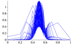
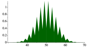
Figure 6: The distributions of the coefficients of A162315: for $n=5,10,\dots,100$ (left) and $n=100$ (right). We see that they are highly oscillating in nature.

Also note specially that despite the oscillating nature of the coefficients (see for example Figure 6), we still have a CLT, which is a global property, not a local one.

The reciprocal polynomials $Q_{n}(v)=v^{n}P_{n}\bigl{(}{\frac{1}{v}}\bigr{)}$ satisfy $Q_{n}\in\mathscr{E}\langle\!\langle 1+v^{2},\frac{v(1+v)}{n-1}\rangle\!\rangle$ with the initial condition $Q_{1}(v)=1+3v$; see A124846. The coefficients of $Q_{n}$ yield the CLT $\mathscr{N}\bigl{(}{\frac{1}{2}n,\frac{1}{4}n}\bigr{)}$.

These two OEIS sequences, together with a few others leading to the same CLT $\mathscr{N}\bigl{(}{\frac{1}{2}n,\frac{1}{4}n}\bigr{)}$, are summarized in the following table. In all cases, it is possible to derive an optimal Berry-Esseen bound but we omit the details because these examples are comparatively simpler (put together here mainly to show the modeling diversity of the Eulerian recurrences).

OEIS	$e_{n}$	Type	$[v^{k}]P_{n}(v)$
A161119	$1$	$\mathscr{E}\langle\!\langle 2vn-v,1+v;1\rangle\!\rangle$	(72)
A161121	$1$	$\mathscr{E}\langle\!\langle(1+v^{2})n-v^{2},v(1+v);1\rangle\!\rangle$	(72)
A162315	$n-1$	$\mathscr{E}_{1}\langle\!\langle 2vn-2v,1+v;3+v\rangle\!\rangle$	$(2-(-1)^{n-k})\binom{n}{k}$
A007318	$n-1$	$\mathscr{E}_{1}\langle\!\langle 2vn-2v,1+v;1+v\rangle\!\rangle$	$\binom{n}{k}$
A124846	$n-1$	$\mathscr{E}_{1}\langle\!\langle(1+v^{2})n-1-v^{2},v(1+v);1+3v\rangle\!\rangle$	$(2-(-1)^{k})\binom{n}{k}$
A121448	$n+2$	$\mathscr{E}\langle\!\langle 4vn+2v,2(1+v);1\rangle\!\rangle$	$\frac{2^{k}}{n+1}\binom{n+1}{k}\binom{n+1-k}{\frac{n-k}{2}}$
A143358	$n+1$	$\mathscr{E}\langle\!\langle 4vn+2,2(1+v);1\rangle\!\rangle$	$2^{k}\binom{n}{k}\binom{n-k}{\lfloor\frac{1}{2}(n-k)\rfloor}$

In particular, the sequence A121448 is also periodic because $\binom{n+1-k}{\frac{n-k}{2}}=0$ when $n-k$ is odd.

On the other hand, the $n$th order derivative of $\sqrt{\frac{1+v}{1-v}}$ leads to the polynomials satisfying the recurrence $P_{n}\in\mathscr{E}\langle\!\langle 2vn+1-2v,1+v;1\rangle\!\rangle$; compare (69). The EGF is given by

$$(1-(1+v)z)^{-\frac{3}{2}}(1+(1-v)z)^{-\frac{1}{2}},$$ (73)

from which we deduce the CLT $\mathscr{N}\bigl{(}{\frac{1}{2}n,\frac{1}{4}n;n^{-\frac{1}{2}}}\bigr{)}$ by Theorem 2 with $\rho(v)=\frac{1}{1+v}$.

5.5.2 $(\alpha(v),\beta(v))=(2(1+v),3+v)\Longrightarrow\mathscr{N}\bigl{(}{\frac{1}{4}n,\frac{3}{16}n}\bigr{)}$

The sequence A091867, which enumerates the number of Dyck paths of semi-length $n$ having $k$ peaks at odd height, has its generating polynomial satisfying the recurrence

$$P_{n}\in\mathscr{E}\left\langle\!\left\langle\frac{2((1+v)n-1)}{n+1},\frac{3+v}{n+1};1\right\rangle\!\right\rangle.$$

A closed-form expression is known (see A091867)

$$[v^{n-k}]P_{n}(v)=\frac{1}{k+1}\binom{n}{k}\sum_{0\leqslant j\leqslant k}(-1)^{j}\binom{k+1}{j}\binom{2k-2j}{k-j}.$$ (74)

Due to the presence of the factor $(-1)^{j}$, the asymptotics of this expression is less transparent; however, we get the CLT $\mathscr{N}\bigl{(}{\frac{1}{4}n,\frac{3}{16}n}\bigr{)}$ by Theorem 1 using the expression of $(\alpha(v),\beta(v))$. The corresponding reciprocal polynomials A124926 satisfy

$$Q_{n}\in\mathscr{E}\left\langle\!\left\langle\frac{(1+3v^{2})n+1-3v^{2}}{n+1},\frac{v(1+3v)}{n+1};1\right\rangle\!\right\rangle.$$

On the other hand, since the ordinary generating function (OGF) of $P_{n-1}$ satisfies

$$\frac{1}{2}-\frac{1}{2}\sqrt{\frac{1-(3+v)z}{1+(1-v)z}},$$ (75)

an optimal Berry-Esseen bound also follows from Theorem 2 with $\rho(v)=\frac{1}{3+v}$. Furthermore, by this OGF we have for $n\geqslant 1$

$$P_{n-1}(v)=\frac{1}{n}[w^{n-1}]\left(1+vw+\frac{w^{2}}{1-w}\right)^{n}.$$

From this and Lagrange inversion formula [225], we derive the expression (without alternating terms; cf. (74))

$$[v^{n-k}]P_{n}(v)=\frac{1}{n+1}\binom{n+1}{k+1}\sum_{0\leqslant j\leqslant\lfloor\frac{1}{2}k\rfloor}\binom{k+1}{j}\binom{k-1-j}{j-1}.$$

Although non-alternating, the asymptotics of the right-hand side still remains obscure.

These sequences and a few others of the same type are listed as follows.

OEIS	$e_{n}$	Type	CLT
A091867	$n+1$	$\mathscr{E}\langle\!\langle(2v+2)n-2,3+v;1\rangle\!\rangle$	$\mathscr{N}\bigl{(}{\frac{1}{4}n,\frac{3}{16}n;n^{-\frac{1}{2}}}\bigr{)}$
A124926	$n+1$	$\mathscr{E}\langle\!\langle(1+3v^{2})n+1-3v^{2},v(1+3v);1\rangle\!\rangle$	$\mathscr{N}\bigl{(}{\frac{3}{4}n,\frac{3}{16}n;n^{-\frac{1}{2}}}\bigr{)}$
A171128	$n$	$\mathscr{E}\langle\!\langle(2v+2)n-1-v,3+v;1\rangle\!\rangle$	$\mathscr{N}\bigl{(}{\frac{1}{4}n,\frac{3}{16}n;n^{-\frac{1}{2}}}\bigr{)}$
A135091	$n$	$\mathscr{E}\langle\!\langle(1+3v^{2})n+v(1-3v),v(1+3v);1\rangle\!\rangle$	$\mathscr{N}\bigl{(}{\frac{3}{4}n,\frac{3}{16}n;n^{-\frac{1}{2}}}\bigr{)}$
A091869	$n+1$	$\mathscr{E}_{1}\langle\!\langle(2v+2)n-1-v,3+v;1\rangle\!\rangle$	$\mathscr{N}\bigl{(}{\frac{1}{4}n,\frac{3}{16}n;n^{-\frac{1}{2}}}\bigr{)}$
A091187	$n+1$	$\mathscr{E}_{1}\langle\!\langle(1+3v^{2})n+1+3v-6v^{2},v(1+3v);1\rangle\!\rangle$	$\mathscr{N}\bigl{(}{\frac{3}{4}n,\frac{3}{16}n;n^{-\frac{1}{2}}}\bigr{)}$
A171651	$n+1$	$\mathscr{E}\langle\!\langle(2v+2)n+2,3+v;1\rangle\!\rangle$	$\mathscr{N}\bigl{(}{\frac{1}{4}n,\frac{3}{16}n;n^{-\frac{1}{2}}}\bigr{)}$

Here the first six are grouped in reciprocal pairs. Each of these has a closed-form expression for their OGFs (as well as a summation formula similar to (74)); we list below only their OGFs.

A171128	$\dfrac{1}{\sqrt{(1-(1-v)z)(1-(3+v)z)}}$
A091869	$\dfrac{1-(1+v)z-\sqrt{(1+(1-v)z)(1-(3+v)z)}}{2z}$
A171651	$\dfrac{1-(3+v)z+\sqrt{(1+(1-v)z)(1-(3+v)z)}}{2(1-(3+v)z)}$

5.5.3 $(\alpha(v),\beta(v))=(q(1+3v),2qv)\Longrightarrow\mathscr{N}\bigl{(}{\frac{1}{2}n,\frac{1}{8}n}\bigr{)}$

The generating polynomials of Narayana numbers (enumerating peaks in Dyck paths; see [230] and A090181)

$$P_{n}(v):=\sum_{1\leqslant k\leqslant n}\frac{1}{k}\binom{n}{k-1}\binom{n-1}{k-1}v^{k}\qquad(n\geqslant 1),$$

also satisfy

$$(n+1)P_{n}(v)=((1+3v)n-1-v)P_{n-1}(v)+2v(1-v)P_{n-1}^{\prime}(v)\qquad(n\geqslant 1)$$ (76)

in addition to the usual three-term recurrence

$$(n+1)P_{n}(v)=(2n-1)(1+v)P_{n-1}(v)-(n-2)(1-v)^{2}P_{n-2}(v).$$

These polynomials are palindromic and the CLT $\mathscr{N}\bigl{(}{\frac{1}{2}n,\frac{1}{8}n}\bigr{)}$ for $[v^{k}]P_{n}(v)$ follows easily from Theorem 1. An essentially identical sequence A001263 corresponds to $v^{-1}P_{n}(v)$. The OGF of $P_{n}$ satisfies

$$f(z,v):=\sum_{n\geqslant 0}P_{n}(v)z^{n}=\frac{1-(1+v)z-\sqrt{1-2(1+v)z+(1-v)^{2}z^{2}}}{2z},$$ (77)

from which we get an additional convergence rate $n^{-\frac{1}{2}}$ by Theorem 2 with $\rho(v)=(1+\sqrt{v})^{-2}$. These and a few others satisfying $P_{n}\in\mathscr{E}\langle\!\langle\frac{(1+3v)n+\gamma(v)}{e_{n}},\frac{2v}{e_{n}}\rangle\!\rangle$, leading to the same CLT $\mathscr{N}\bigl{(}{\frac{1}{2}n,\frac{1}{8}n;n^{-\frac{1}{2}}}\bigr{)}$, are collected in the following table.

OEIS	$e_{n}$	Type	$[v^{k}]P_{n}(v)$
A086645	$n-1$	$\mathscr{E}_{1}\langle\!\langle(1+3v)(n-1),2v;1+v\rangle\!\rangle$	$\binom{2n}{2k}$
A103328	$n-1$	$\mathscr{E}_{1}\langle\!\langle(1+3v)n-4v,2v;2\rangle\!\rangle$	$\binom{2n}{2k+1}$
A091044	$n$	$\mathscr{E}\langle\!\langle(1+3v)n+1-v,2v;1\rangle\!\rangle$	$\frac{1}{2}\binom{2n}{2k+1}$
A001263	$n+1$	$\mathscr{E}\langle\!\langle(1+3v)n-1-v,2v;1\rangle\!\rangle$	$\frac{1}{k}\binom{n}{k-1}\binom{n-1}{k-1}$
A090181	$n+1$	$\mathscr{E}\langle\!\langle(1+3v)n-1-v,2v;1\rangle\!\rangle$	$\frac{1}{k}\binom{n}{k-1}\binom{n-1}{k-1}$
A131198	$n+1$	$\mathscr{E}\langle\!\langle(1+3v)n+1-3v,2v;1\rangle\!\rangle$	$\frac{1}{n-k}\binom{n}{k+1}\binom{n-1}{k}$
A118963	$n$	$\mathscr{E}_{1}\langle\!\langle(1+3v)n+1-3v,2v;2\rangle\!\rangle$	$\frac{n+1}{n}\binom{n}{k}\binom{n}{k+1}$
A008459	$n$	$\mathscr{E}\langle\!\langle(1+3v)n-2v,2v;1\rangle\!\rangle$	$\binom{n}{k}^{2}$

In particular, we see that the coefficients $\binom{n}{k}^{2}$ follow asymptotically a CLT $\mathscr{N}\bigl{(}{\frac{1}{2}n,\frac{1}{8}n}\bigr{)}$, the variance being smaller than that of $\binom{n}{k}$; more generally, $\binom{n}{k}^{\alpha}$ follows asymptotically the CLT $\mathscr{N}\bigl{(}{\frac{1}{2}n,\frac{1}{4\alpha}n}\bigr{)}$ for large $n$ when $\alpha>0$; see Figure 7.

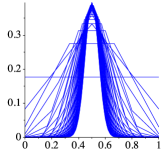
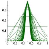
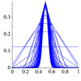
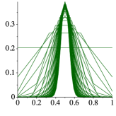
Figure 7: Normalized histograms of $\binom{n}{k}^{\alpha}$ for $n=1,\dots,50$ and $\alpha=2,3,4$ (the first three), respectively, and the Eulerian distribution (rightmost). The variance for the second and the fourth are both asymptotic to $\frac{1}{12}n$. Note that $\binom{n}{k}^{3}$ correspond to A181543 and $\binom{n}{k}^{4}$ to A202750.

While the generating polynomials of $\binom{2n}{2k}$ satisfy (76), those of $\binom{2n+1}{2k}$ and $\binom{2n+1}{2k+1}$ satisfy the following recurrences

A091042	$\binom{2n+1}{2k}$	$\mathscr{E}\langle\!\langle\frac{2(1+3v)n-1-3v}{2n-1},\frac{4v}{2n-1};1\rangle\!\rangle$
A103327	$\binom{2n+1}{2k+1}$	$\mathscr{E}\langle\!\langle\frac{2(1+3v)n+1-5v}{2n-1},\frac{4v}{2n-1};1\rangle\!\rangle$

The two sequences form a reciprocal pair.

5.5.4 $(\alpha(v),\beta(v))=(5+3v,2(1+v))\Longrightarrow\mathscr{N}\bigl{(}{\frac{1}{4}n,\frac{5}{32}n}\bigr{)}$

The polynomials (A114608, enumerating the number of peaks in bicolored Dyck paths)

$$P_{n}(v)=\frac{1}{n}\sum_{0\leqslant k\leqslant n}v^{k}\sum_{0\leqslant j\leqslant n-k}\binom{n}{j+1}\binom{n-k}{j}2^{j},$$

satisfy $P_{n}\in\mathscr{E}\langle\!\langle\frac{(5+3v)n-3-v}{n+1},\frac{2(1+v)}{n+1};1\rangle\!\rangle$. The CLT $\mathscr{N}\bigl{(}{\frac{1}{4}n,\frac{5}{32}n}\bigr{)}$ then follows from Theorem 1, and an effective version with $n^{-\frac{1}{2}}$ convergence rate follows from Theorem 2 using the OGF

$$\frac{1+(1-v)z-\sqrt{1-2(3+v)z+(1-v)^{2}z^{2}}}{4z},$$ (78)

with $\rho(v)=\bigl{(}{\sqrt{2}+\sqrt{1+v}}\bigr{)}^{-2}$.

5.5.5 $(\alpha(v),\beta(v))=\bigl{(}{\frac{1}{3}(7+2v),\frac{1}{3}(5+4v)}\bigr{)}\Longrightarrow\mathscr{N}\bigl{(}{\frac{1}{9}n,\frac{2}{27}n}\bigr{)}$

The generating polynomial (A181371) of the pattern occurrences of “$01$” in ternary words satisfies $P_{n}\in\mathscr{E}\langle\!\langle\frac{(7+2v)n+2(1-v)}{3n},\frac{5+4v}{3n};1\rangle\!\rangle$. This follows from the OGF

$$\sum_{n\geqslant 0}P_{n}(v)z^{n}=\frac{1}{1-3z+(1-v)z^{2}}.$$ (79)

From this we deduce the CLT $\mathscr{N}\bigl{(}{\frac{1}{9}n,\frac{2}{27}n;n^{-\frac{1}{2}}}\bigr{)}$ for the coefficients $[v^{k}]P_{n}(v)$ by Theorem 2 with $\rho(v)=\frac{2}{3+\sqrt{5+4v}}$.

5.5.6 $(\alpha(v),\beta(v))=(1+3v^{2},v(1+v))\Longrightarrow\mathscr{N}\bigl{(}{n,\frac{1}{2}n}\bigr{)}$

The sequence A088459 enumerates peaks in symmetric Dyck paths and the corresponding polynomials satisfy $\mathscr{E}\langle\!\langle\frac{(1+3v^{2})n+1+v}{n+1},\frac{v(1+v)}{n+1};1+v\rangle\!\rangle$. One then gets the CLT $\mathscr{N}\bigl{(}{n,\frac{1}{2}n}\bigr{)}$ by Theorem 1. This and a few other polynomials from OEIS are listed as follows.

A088459	Peaks in symmetric Dyck paths	$\mathscr{E}\langle\!\langle\frac{(1+3v^{2})n+1+v}{n+1},\frac{v(1+v)}{n+1};1+v\rangle\!\rangle$
A059064	Card-matching numbers	$\mathscr{E}\langle\!\langle\frac{(1+3v^{2})n-2v^{2}}{n},\frac{v(1+v)}{n};1\rangle\!\rangle$
A059065	Card-matching numbers	$\mathscr{E}\langle\!\langle(1+3v^{2})n^{2}-2v^{2}n,v(1+v)n;1\rangle\!\rangle$
A152659	Turns in lattice paths	$\mathscr{E}\langle\!\langle\frac{(1+3v^{2})n+1+2v-v^{2}}{n+1},\frac{v(1+v)}{n+1};2\rangle\!\rangle$
A247644	Even rows of A088855	$\mathscr{E}\langle\!\langle\frac{(1+3v^{2})n+1+2v-v^{2}}{n+1},\frac{v(1+v)}{n+1};1\rangle\!\rangle$

A convergence rate in the CLT can be obtained by solving the corresponding PDEs and then by applying Theorem 2. For example, the OGF for A152659 is given by

$$\frac{2}{z(v-f(z,v^{2}))}-\frac{2}{vz},$$ (80)

where $f$ is the generating function (77) of Narayana numbers. Thus $\rho(v)=(1+v)^{-2}$ and the CLT $\mathscr{N}\bigl{(}{n,\frac{1}{2}n;n^{-\frac{1}{2}}}\bigr{)}$ is implied.

5.6 Polynomials with $(\alpha(v),\beta(v))=(-1+(q+1)v,qv)\Longrightarrow\mathscr{N}\bigl{(}{\frac{q+1}{2q}\,n,\frac{q^{2}-1}{12q^{2}}\,n}\bigr{)}$

A generalization of Morisita’s model (45) proposed by Charalambides and Koutras in [45] is of the form

$$P_{n}\in\mathscr{E}\left\langle\!\left\langle\frac{(-1+(q+1)v)n+1+p+(qr-p-q-1)v}{n},\frac{qv}{n};1\right\rangle\!\right\rangle.$$

The OGF $f(z,v):=\sum_{n\geqslant 0}P_{n}(v)z^{n}$ is given by

$$\bigl{(}{1+(1-v)z}\bigr{)}^{p}\left(\frac{1-v}{1-v(1+(1-v)z)^{q}}\right)^{r}.$$ (81)

We write this class as $f\in\mathscr{M}(p,q,r)$ or $f\in\mathscr{M}(p,q,r;z)$. The type $\mathscr{M}(p,q,1)$ was studied in [41], and the type $\mathscr{M}\bigl{(}{\frac{p}{q},\frac{1}{q},1;qz}\bigr{)}$ in [132] in connection with degenerate Stirling numbers. It is interesting to compare these forms with those ((37) and (38)) for $\mathscr{A}(p,q,r)$ where the factor “$e^{(1-v)z}$” there is “mimicked” by “$1+(1-v)z$” here. If $[v^{k}]P_{n}(v)\geqslant 0$ or $(-1)^{n}[v^{k}]P_{n}(v)\geqslant 0$ and $|q|>1$, then we obtain the CLT $\mathscr{N}\bigl{(}{\frac{q+1}{2q}n,\frac{q^{2}-1}{12q^{2}}n}\bigr{)}$ for the coefficients by Theorem 1 and $\mathscr{N}\bigl{(}{\frac{q+1}{2q}n,\frac{q^{2}-1}{12q^{2}}n;n^{-\frac{1}{2}}}\bigr{)}$ by Theorem 2 with $\rho(v)=-\frac{1-v^{-\frac{1}{q}}}{1-v}$.

The reciprocal polynomial $Q_{n}(v):=v^{n}P_{n}\bigl{(}{\frac{1}{v}}\bigr{)}$ satisfies

$$Q_{n}\in\mathscr{E}\left\langle\!\left\langle\frac{(1+(q-1)v)n+qr-1-p+(1+p-q)v}{n},\frac{qv}{n};1\right\rangle\!\right\rangle.$$

This gives the pair $(\alpha(v),\beta(v))=(1+(q-1)v,qv)$, and then the CLT $\mathscr{N}\bigl{(}{\frac{q-1}{2q}\,n,\frac{q^{2}-1}{12q^{2}}\,n;n^{-\frac{1}{2}}}\bigr{)}$. If $f\in\mathscr{M}(p,q,r;z)$, then the reciprocal polynomial is of type $\mathscr{M}(p-qr,-q,r;-z)$.

Runs in words: $\mathscr{M}(0,q,1;z)$ or $\mathscr{M}(-q,-q,1;-z)$

This class of polynomials appeared in Carlitz’s study [32, 33] of “degenerate” Eulerian numbers (which corresponds to $\mathscr{M}(0,q,1;\frac{z}{q})$), as well as that of rises in sequences (with repetitions) [36], and was later referred to as the Carlitz numbers in [43, §14.3]. Such numbers also enumerate increasing runs in $q$-ary words and have the closed-form expression

$$P_{n}(v)=\sum_{0\leqslant k\leqslant n}v^{k}\sum_{0\leqslant j\leqslant k}(-1)^{k-j}\binom{n+1}{k-j}\binom{qj}{n};$$

see also [69] for the occurrence of these numbers in algebraic geometry. Note that when $q=2$, one gets the simpler expression $\binom{n+1}{2n-2k+1}$ for $[v^{k}]P_{n}(v)$. We obtain the CLT $\mathscr{N}\bigl{(}{\frac{q+1}{2q}\,n,\frac{q^{2}-1}{12q^{2}}\,n;n^{-\frac{1}{2}}}\bigr{)}$ when $q>1$ is an integer. When $q=1$, we get the OGF $\frac{1}{1-vz}$, and the limit law is degenerate. The cases $q=2,3,4$ appear in OEIS:

Description	OEIS	Type	CLT
$\uparrow$ runs in binary words	A119900	$\mathscr{M}(0,2,1;z)$	$\mathscr{N}\bigl{(}{\frac{3}{4}n,\frac{1}{16}n;n^{-\frac{1}{2}}}\bigr{)}$
A119900 without zeros	A109447		$\mathscr{N}\bigl{(}{\frac{1}{4}n,\frac{1}{16}n;n^{-\frac{1}{2}}}\bigr{)}$
Reciprocal of A119900	A202064	$\mathscr{M}(-2,-2,1;-z)$	$\mathscr{N}\bigl{(}{\frac{1}{4}n,\frac{1}{16}n;n^{-\frac{1}{2}}}\bigr{)}$
A202064 without zeros	A034867		$\mathscr{N}\bigl{(}{\frac{1}{4}n,\frac{1}{16}n;n^{-\frac{1}{2}}}\bigr{)}$
$\uparrow$ runs in ternary words	A120987	$\mathscr{M}(0,3,1;z)$	$\mathscr{N}\bigl{(}{\frac{2}{3}n,\frac{2}{27}n;n^{-\frac{1}{2}}}\bigr{)}$
Reciprocal of A120987	A120906	$\mathscr{M}(-3,-3,1;-z)$	$\mathscr{N}\bigl{(}{\frac{1}{3}n,\frac{2}{27}n;n^{-\frac{1}{2}}}\bigr{)}$
$\uparrow$ runs in quaternary words	A265644	$\mathscr{M}(0,4,1;z)$	$\mathscr{N}\bigl{(}{\frac{5}{8}n,\frac{5}{64}n;n^{-\frac{1}{2}}}\bigr{)}$

Patterns in words: $\mathscr{M}(1,2,1)$

Similar to the numbers A119900 above, we also have the following variants for the sequence $\binom{n}{2k}$.

Description	OEIS	Type	CLT
$\binom{n}{2n-2k}$	A098158	$1+vz\mathscr{M}(1,2,1;z)$	$\mathscr{N}\bigl{(}{\frac{3}{4}n,\frac{1}{16}n;n^{-\frac{1}{2}}}\bigr{)}$
$2\binom{n}{2k}$	A119462	$2\mathscr{M}(-1,-2,1;-z)$	$\mathscr{N}\bigl{(}{\frac{3}{4}n,\frac{1}{16}n;n^{-\frac{1}{2}}}\bigr{)}$
shifted version of A098158	A098157	$\mathscr{M}(1,2,1;z)$	$\mathscr{N}\bigl{(}{\frac{3}{4}n,\frac{1}{16}n;n^{-\frac{1}{2}}}\bigr{)}$
A098158 without zeros	A109446		$\mathscr{N}\bigl{(}{\frac{3}{4}n,\frac{1}{16}n;n^{-\frac{1}{2}}}\bigr{)}$
Reciprocal of A098158	A202023	$\mathscr{M}(-1,-2,1;-z)$	$\mathscr{N}\bigl{(}{\frac{1}{4}n,\frac{1}{16}n;n^{-\frac{1}{2}}}\bigr{)}$
A202023 without zeros	A034839		$\mathscr{N}\bigl{(}{\frac{1}{4}n,\frac{1}{16}n;n^{-\frac{1}{2}}}\bigr{)}$

Binomial extension of Eulerian numbers: $\mathscr{M}(p,q,1)$

This class was studied in [41, 154], where occurrences and applications are mentioned.

Description	OEIS	Type	CLT
$(1-v)^{n+1}\sum_{j\geqslant 0}\binom{3j+n}{n}v^{j}$	A178618	$\mathscr{M}(-1,-3,1;-z)$	$\mathscr{N}\bigl{(}{\frac{1}{3}n,\frac{2}{27}n;n^{-\frac{1}{2}}}\bigr{)}$
$(1-v)^{n+1}\sum_{j\geqslant 0}\binom{4j+n}{n}v^{j}$	A178619	$\mathscr{M}(-1,-4,1;-z)$	$\mathscr{N}\bigl{(}{\frac{3}{8}n,\frac{5}{64}n;n^{-\frac{1}{2}}}\bigr{)}$

In general, the polynomials $(1-v)^{n+1}\sum_{j\geqslant 0}\binom{qj+n}{n}v^{j}$ are of type $\mathscr{M}(-1,-q,1;-z)$ for any real $q$, and one obtains the CLT $\mathscr{N}\bigl{(}{\frac{q+1}{2q}\,n,\frac{q^{2}-1}{12q^{2}}\,n;n^{-\frac{1}{2}}}\bigr{)}$ when $q\geqslant 2$ is an integer.

Degenerate limit law: $\mathscr{M}(2,1,3)$

Consider A106246 for which $a_{n,k}=\binom{n}{k}\binom{2}{n-k}$. Then $P_{n}\in\mathscr{E}\langle\!\langle\frac{(2v-1)n+3-v}{n},\frac{v}{n};1\rangle\!\rangle$. This is of type $\mathscr{M}(2,1,3)$. Of course, the random variable $X_{n}$ is degenerate or follows in the limit the Dirac distribution. The reciprocal polynomials $Q_{n}(v):=v^{n}P_{n}\bigl{(}{\frac{1}{v}}\bigr{)}$ satisfies $Q_{n}\in\mathscr{E}\langle\!\langle n+2v,v;1\rangle\!\rangle$. This is of the type of problems we will examine in the next three sections.

Finally, for $\mathscr{M}(p,1,r)$, the GF becomes

$$\frac{(1+(1-v)z)^{p}}{(1-vz)^{r}},$$

which has nonnegative coefficients when $0\leqslant p\leqslant r$.

See Section 9.5 for a sequence of polynomials closely related to $\mathscr{M}(0,2,\frac{3}{2})$.

6 Non-normal limit laws

We now work out the method of moments for the recurrence (9) when the limit laws are not normal. It turns out all examples we found are of the simpler form

$$P_{n}\in\mathscr{E}\left\langle\!\left\langle\frac{\alpha n+\gamma+\gamma^{\prime}(v-1)}{e_{n}},\frac{\beta+\beta^{\prime}(v-1)}{e_{n}};c_{0}+c_{1}(v-1)\right\rangle\!\right\rangle,$$ (82)

which are polynomials in $v$ of degree at most $n+1$, where $\alpha,\beta,\beta^{\prime}\gamma,\gamma^{\prime}$ are constants (often integers) and $\{e_{j}\}_{j\geqslant 1}$ is a positive sequence. For this framework, if we apply naively Theorem 1 (after normalizing by $\prod_{1\leqslant j\leqslant n}e_{j}$), then we see that $\mu=\sigma^{2}=0$ (since $\alpha(v)=\alpha$ is a constant); thus Theorem 1 fails but we will see that the same method of proof still applies.

It is also possible to apply the complex-analytic approach to all cases we discuss here and quantify the convergence rates and even the asymptotic densities, but we omit this approach here for brevity and for the following reasons: first, the EGFs or OGFs of $P_{n}$ under (82) are comparatively simpler than those in the case of normal limit laws and the application of singularity analysis is straightforward; second, the method of moments does not rely on the availability of more tractable EGFs or OGFs and is completely elementary and to some extent more general, although the limit results are generally weaker and less easy to be further strengthened.

6.1 Recurrence for the factorial moments

Throughout this section, let $P_{n}$ be defined by (82). Assume that

$$[v^{k}]P_{n}(v)\geqslant 0\text{ for all }k,n\geqslant 0\text{ and }P_{0}(1)=c_{0}>0,\alpha>0,\alpha+\gamma>0,$$ (83)

which then implies, by the relation

$$P_{n}(1)=P_{0}(1)\prod_{1\leqslant j\leqslant n}\frac{\alpha j+\gamma}{e_{j}},$$

that $P_{n}(1)>0$ for $n\geqslant 1$. Since the coefficients are nonnegative and $P_{n}(1)>0$, we define the random variables $X_{n}$ as in (10). In particular, $P_{0}(0)=c_{0}-c_{1}\geqslant 0$, implying that $\frac{c_{1}}{c_{0}}\in[0,1]$.

For convenience, introduce, throughout this section, the notations

$$\tau_{1}:=-\frac{\beta}{\alpha},\quad\tau_{2}:=\frac{\gamma}{\alpha},\quad\text{and}\quad\tau_{3}:=-\frac{\gamma^{\prime}}{\beta^{\prime}}.$$ (84)

Here $\tau_{3}$ is defined when $\beta^{\prime}\neq 0$, and by (83), $1+\tau_{2}>0$.

To compute the factorial moments of $X_{n}$, we rewrite (82) as

$$\mkern 1.5mu\overline{\mkern-1.5muP\mkern-1.5mu}\mkern 1.5mu_{n}(t):=\frac{P_{n}(1+t)}{P_{n}(1)}=\frac{\alpha n+\gamma+\gamma^{\prime}t}{\alpha n+\gamma}\,\mkern 1.5mu\overline{\mkern-1.5muP\mkern-1.5mu}\mkern 1.5mu_{n-1}(t)-\frac{t(\beta+\beta^{\prime}t)}{\alpha n+\gamma}\,\mkern 1.5mu\overline{\mkern-1.5muP\mkern-1.5mu}\mkern 1.5mu_{n-1}^{\prime}(t),$$

with $\mkern 1.5mu\overline{\mkern-1.5muP\mkern-1.5mu}\mkern 1.5mu_{0}(t)=1+\frac{c_{1}}{c_{0}}t$.

Lemma 4.

Let $\mkern 1.5mu\overline{\mkern-1.5muP\mkern-1.5mu}\mkern 1.5mu_{n,m}:=\mkern 1.5mu\overline{\mkern-1.5muP\mkern-1.5mu}\mkern 1.5mu_{n}^{(m)}(0)$ denote the $m$-th factorial moment of $X_{n}$. Then for $n,m\geqslant 1$

$$\mkern 1.5mu\overline{\mkern-1.5muP\mkern-1.5mu}\mkern 1.5mu_{n,m}=\left(1+\frac{m\tau_{1}}{n+\tau_{2}}\right)\mkern 1.5mu\overline{\mkern-1.5muP\mkern-1.5mu}\mkern 1.5mu_{n-1,m}+\frac{m(\gamma^{\prime}-(m-1)\beta^{\prime})}{\alpha(n+\tau_{2})}\,\mkern 1.5mu\overline{\mkern-1.5muP\mkern-1.5mu}\mkern 1.5mu_{n-1,m-1},$$ (85)

with the initial conditions $\mkern 1.5mu\overline{\mkern-1.5muP\mkern-1.5mu}\mkern 1.5mu_{n,0}=1$, $\mkern 1.5mu\overline{\mkern-1.5muP\mkern-1.5mu}\mkern 1.5mu_{0,1}=\frac{c_{1}}{c_{0}}$, and $\mkern 1.5mu\overline{\mkern-1.5muP\mkern-1.5mu}\mkern 1.5mu_{0,m}=0$ for $m\geqslant 2$.

Asymptotics of the mean

By solving (85) for $m=1$, we obtain the following exact expression for the mean $\mkern 1.5mu\overline{\mkern-1.5muP\mkern-1.5mu}\mkern 1.5mu_{n,1}$.

Lemma 5.

Let $n_{0}\geqslant 0$ be the largest $n$ for which $n+\tau_{1}+\tau_{2}=0$; let $n_{0}=0$ if no such $n$ exists. Then the expected value $\mathbb{E}(X_{n})=\mkern 1.5mu\overline{\mkern-1.5muP\mkern-1.5mu}\mkern 1.5mu_{n,1}$ of $X_{n}$ satisfies for $n>n_{0}$

$$\mathbb{E}(X_{n})=\frac{\gamma^{\prime}}{\beta}+\left(\mathbb{E}(X_{n_{0}})-\frac{\gamma^{\prime}}{\beta}\right)\frac{\Gamma\bigl{(}{n+\tau_{1}+\tau_{2}+1}\bigr{)}\Gamma\bigl{(}{n_{0}+\tau_{2}+1}\bigr{)}}{\Gamma\bigl{(}{n+\tau_{2}+1}\bigr{)}\Gamma\bigl{(}{n_{0}+\tau_{1}+\tau_{2}+1}\bigr{)}}.$$ (86)

It turns out that the sign of $\tau_{1}$ is crucial in determining the type of the limit law being discrete or continuous in almost all cases we discuss.

Corollary 5.

If $\beta>0$ (or $\tau_{1}<0$), then

$$\mathbb{E}(X_{n})=\frac{\gamma^{\prime}}{\beta}+O\bigl{(}{n^{\tau_{1}}}\bigr{)};$$

if $\beta<0$ (or $\tau_{1}>0$), then

$$\mathbb{E}(X_{n})=\left(\frac{c_{1}}{c_{0}}-\frac{\gamma^{\prime}}{\beta}\right)\frac{\Gamma\bigl{(}{\tau_{2}+1}\bigr{)}}{\Gamma\bigl{(}{\tau_{1}+\tau_{2}+1}\bigr{)}}\,n^{\tau_{1}}+O\left(1+n^{\tau_{1}-1}\right).$$

Proof.

When $\tau_{1}>0$, we can take $n_{0}=0$ because of the condition $1+\tau_{1}>0$ (or $\alpha+\gamma>0$) in (83). Then the approximations in both cases follow directly from (86) and $\mathbb{E}(X_{0})=\frac{c_{1}}{c_{0}}$. ∎

The discussion of the special case when $\beta=0$ is simpler and deferred to Section 10.

Note specially that in the first case of positive $\beta$ the dominant term is independent of the initial values $c_{0}$ and $c_{1}$, and so are all moments, as well as the limit law, as we will see later, in contrast to the negative $\beta$ case in which all moments asymptotics and the limit law depend critically on the initial values.

Dependence of the parameters

From Corollary 5 and the nonnegativity of the coefficients $[v^{k}]P_{n}(v)$ (and the mean), we obtain the following relations.

Corollary 6.

If $\beta>0$, then $\gamma^{\prime}\geqslant 0$; if $\beta<0$, then $\gamma^{\prime}\geqslant\frac{c_{1}}{c_{0}}\beta$.

More relations among the variables can be derived.

Lemma 6.

Assume that the relations (83) hold. If $\beta^{\prime}>0$, then $\gamma^{\prime}=\ell\beta^{\prime}$ for some positive integer $\ell$; if $\beta^{\prime}<0$, then $\gamma^{\prime}\geqslant\beta^{\prime}$ (or $\tau_{3}\geqslant-1$).

Proof.

Consider first $\beta^{\prime}>0$. By the expression

$$[v^{n+1}]P_{n}(v)=c_{1}\prod_{1\leqslant j\leqslant n}\frac{\gamma^{\prime}-j\beta^{\prime}}{e_{j}}\qquad(n\geqslant 1),$$

and the nonnegativity of $[v^{k}]P_{n}(v)$ for all $k$, we deduce that $\gamma^{\prime}=\ell\beta^{\prime}$ for some positive integer $\ell$. Similarly, if $\beta^{\prime}<0$, then by induction $\gamma^{\prime}\geqslant\beta^{\prime}$. ∎

The situation when $\gamma^{\prime}=\beta^{\prime}$ (or $\tau_{3}=-1$) leads to a Bernoulli limit law; see Theorem 5 below.

Solution to the recurrence

We prove in what follows that the factorial moments in the first case ($\tau_{1}<0$) are all bounded, leading to a discrete limit law, and that those in the second case ($\tau_{1}>0$) all behave like powers of the mean, yielding mostly a continuous limit law.

For higher moments, we consider the following recurrence, which is Lemma 2 but specially formatted in the current setting.

Lemma 7.

Let $n_{0}\geqslant 0$ be the largest $n$ for which $n+m\tau_{1}+\tau_{2}=0$; let $n_{0}=0$ if no such $n$ exists. Then the solution to the recurrence

$$x_{n}=\left(1+\frac{m\tau_{1}}{n+\tau_{2}}\right)x_{n-1}+\frac{y_{n}}{\alpha(n+\tau_{2})}\qquad(n\geqslant n_{0}+1;m\geqslant 0),$$ (87)

with $x_{n_{0}}\neq 0$ is given by

$$\begin{split}x_{n}&=x_{n_{0}}\frac{\Gamma\bigl{(}{n+m\tau_{1}+\tau_{2}+1}\bigr{)}\Gamma(n_{0}+\tau_{2}+1)}{\Gamma\bigl{(}{n+\tau_{2}+1}\bigr{)}\Gamma(n_{0}+m\tau_{1}+\tau_{2}+1)}\\ &\qquad+\frac{\Gamma\bigl{(}{n+m\tau_{1}+\tau_{2}+1}\bigr{)}}{\alpha\Gamma\bigl{(}{n+\tau_{2}+1}\bigr{)}}\sum_{n_{0}<k\leqslant n}\frac{y_{k}\Gamma\bigl{(}{k+\tau_{2}}\bigr{)}}{\Gamma\bigl{(}{k+m\tau_{1}+\tau_{2}+1}\bigr{)}}.\end{split}$$ (88)

Starting with the recurrence (85) and the mean, we can derive asymptotic approximations to $\mkern 1.5mu\overline{\mkern-1.5muP\mkern-1.5mu}\mkern 1.5mu_{n,m}$ successively by induction for $m\geqslant 2$, and then conclude the limit laws by the method of moments. Unlike normal limit laws, there is no need to center the random variables, which makes the calculations simpler; however, the expressions for the limiting moments are generally more involved (than those in the normal cases).

6.2 EGF and PDE

The recurrence (82) (for $n\geqslant 1$ with with $P_{0}(v)=c_{0}+c_{1}(v-1)$) leads to the PDE satisfied by the EGF of $P_{n}$

$$(1-\alpha z)F_{z}^{\prime}-(\beta-\beta^{\prime}(1-v))(1-v)F_{v}^{\prime}-(\alpha+\gamma-\gamma^{\prime}(1-v))F=0,$$

where $F(z,v):=\sum_{n\geqslant 0}\frac{P_{n}(v)}{n!}\,z^{n}$. The solution can be derived by the standard procedure described in Section 3.1.

Proposition 2.

Assume $\alpha>0$ and $\beta\neq 0$. The EGF of $P_{n}$ (satisfying (82)) is given as follows.

• If $\beta^{\prime}=0$, then

  $$F(z,v)=(1-\alpha z)^{-\frac{\alpha+\gamma}{\alpha}}e^{-\frac{\gamma^{\prime}}{\beta}(1-v)(1-(1-\alpha z)^{\frac{\beta}{\alpha}})}\left(c_{0}-c_{1}(1-v)(1-\alpha z)^{\frac{\beta}{\alpha}}\right).$$ (89)

• If $\beta^{\prime}\neq 0$, then

  $$F(z,v)=\frac{c_{0}(\beta-\beta^{\prime}(1-v))+(c_{0}\beta^{\prime}-c_{1}\beta)(1-v)(1-\alpha z)^{\frac{\beta}{\alpha}}}{\beta(1-\alpha z)^{\frac{\alpha+\gamma}{\alpha}}\Bigl{(}{\frac{\beta-\beta^{\prime}(1-v)+\beta^{\prime}(1-v)(1-\alpha z)^{\frac{\beta}{\alpha}}}{\beta}}\Bigr{)}^{1-\frac{\gamma^{\prime}}{\beta^{\prime}}}}.$$ (90)

Note that (89) also follows from (90) by taking the limit as $\beta^{\prime}\to 0$. Also if $\beta^{\prime}=0$, then $\beta>0$ because otherwise the coefficients are not all nonnegative. By varying the seven parameters, the simple solution (90) is capable of generating many different non-normal limit laws, as we will examine in the next two sections but instead by an elementary approach.

6.3 Discrete limit laws

We consider in this subsection the case when the limit law is discrete, which arises mostly when $\beta>0$, beginning with the following asymptotic transfer.

Lemma 8.

Assume that $x_{n}$ satisfies (87) with $m\geqslant 1$ and $\tau_{1}<0$. Then

$$y_{n}\sim K\quad\text{implies that}\quad x_{n}\sim\frac{K}{m\beta}.$$ (91)

Proof.

By (88) using the asymptotic approximation (25) to the ratio of Gamma functions. ∎

Recall that $\tau_{3}=-\frac{\gamma^{\prime}}{\beta^{\prime}}$; see (84).

Proposition 3.

Assume $\tau_{1}<0$ (or $\beta>0$). Then the $m$-th factorial moment of $X_{n}$ satisfies

$$\mathbb{E}(X_{n}^{\underline{m}})\sim K_{m}:=\begin{cases}\displaystyle\biggl{(}{\frac{\gamma^{\prime}}{\beta}}\biggr{)}^{m},&\text{if }\beta^{\prime}=0\\ \displaystyle\frac{\Gamma(m+\tau_{3})}{\Gamma(\tau_{3})}\left(-\frac{\beta^{\prime}}{\beta}\right)^{m},&\text{if }\beta^{\prime}<0\\ \displaystyle\frac{\ell!}{(\ell-m)!}\left(\frac{\beta^{\prime}}{\beta}\right)^{m},&\text{if }\beta^{\prime}>0,\gamma^{\prime}=\ell\beta^{\prime},\end{cases}$$ (92)

for $m\geqslant 0$, where $x^{\underline{m}}:=\prod_{0\leqslant j<m}(x-j)$.

Proof.

By the recurrence (85), the asymptotic transfer (91) and induction. ∎

By Corollary 6, since $\beta>0$, we have $\gamma^{\prime}>0$ in all cases of $\beta^{\prime}$.

Theorem 5 ($\beta>0\Longrightarrow$ discrete limit laws).

Let $P_{n}(v)$ be defined by the recurrence (82). Assume that (i) $[v^{k}]P_{n}(v)\geqslant 0$ for $k,n\geqslant 0$, (ii) $P_{n}(1)>0$ for $n\geqslant 0$, and (iii) $\beta>0$. Define $X_{n}$ by $\mathbb{E}(v^{X_{n}}):=\frac{P_{n}(v)}{P_{n}(1)}$. Then

• if $\beta^{\prime}=0$, then $X_{n}$ follows asymptotically a Poisson distribution with parameter $\frac{\gamma^{\prime}}{\beta}$;

• if $\beta^{\prime}<0$, then $X_{n}$ follows asymptotically a negative binomial distribution with parameters $\tau_{3}$ and $-\frac{\beta^{\prime}}{\beta-\beta^{\prime}}$;

• if $\beta^{\prime}>0$, $\beta^{\prime}<\beta$ and $\gamma^{\prime}=\ell\beta^{\prime}$ for $\ell=1,2,\dots$, then $X_{n}$ is the sum of $\ell$ independent and identically distributed Bernoulli random variables with parameter $\frac{\beta^{\prime}}{\beta}$ (or binomial with parameters $\ell$ and $\frac{\beta^{\prime}}{\beta}$).

Proof.

If $\beta^{\prime}=0$, then by Proposition 3, we see that the probability generating function of the limit law equals $e^{\frac{\gamma^{\prime}}{\beta}(v-1)}$, which is nothing but that of a Poisson random variable with mean $\frac{\gamma^{\prime}}{\beta}$.

Now if $\beta^{\prime}<0$, then $\tau_{3}>0$ (since $\gamma^{\prime}>0$), and the variance is asymptotic to $\frac{(\beta-\beta^{\prime})\gamma^{\prime}}{\beta^{2}}$ in this case. By (92), we deduce that the probability generating function of the limit law equals

$$\bigl{(}1+\tfrac{\beta^{\prime}}{\beta}(v-1)\bigr{)}^{-\tau_{3}},$$

so we get a negative binomial with parameters $\tau_{3}$ and $-\frac{\beta^{\prime}}{\beta-\beta^{\prime}}\in(0,1)$.

Finally, if $\beta^{\prime}>0,\beta\neq\beta^{\prime}$ and $\gamma^{\prime}=\ell\beta^{\prime}$, then we obtain the probability generating function $\bigl{(}{1+\frac{\beta^{\prime}}{\beta}(v-1)}\bigr{)}^{\ell}$, which is the sum of $\ell$ Bernoulli random variables with mean $\frac{\beta^{\prime}}{\beta}$. ∎

6.4 Continuous limit laws

The case when $\tau_{1}>0$ ($\beta<0$) is phenomenally more interesting as the underlying random variables have generally a wider range of variations. We may without loss of generality assume that $\beta^{\prime}<0$ because otherwise the coefficients $[v^{k}]P_{n}(v)$ are not all nonnegative. From Lemma 6, we see that $\tau_{3}>-1$ (the equality being already covered by Theorem 5). We derive first the asymptotics of the factorial moments.

Proposition 4.

Assume $\tau_{1}>0$ ($\beta<0$). Then the $m$th moment of $X_{n}$ is asymptotic to

$$\mathbb{E}\left(\frac{X_{n}}{\frac{\beta^{\prime}}{\beta}\,n^{\tau_{1}}}\right)^{m}\sim\mathbb{E}\left(\frac{X_{n}}{\frac{\beta^{\prime}}{\beta}\,n^{\tau_{1}}}\right)^{\underline{m}}\sim K_{m}\qquad(m\geqslant 0),$$ (93)

where

$$K_{m}=\frac{\Gamma\bigl{(}{m+\tau_{3}}\bigr{)}\Gamma(\tau_{2}+1)}{\Gamma\bigl{(}{\tau_{3}+1}\bigr{)}\Gamma\bigl{(}{m\tau_{1}+\tau_{2}+1}\bigr{)}}\left(\frac{c_{1}\beta}{c_{0}\beta^{\prime}}\,m+\tau_{3}\right)\qquad(m\geqslant 0).$$ (94)

Proof.

We prove the second estimate of (93) by induction. Assume that the $m$th factorial moment $\mkern 1.5mu\overline{\mkern-1.5muP\mkern-1.5mu}\mkern 1.5mu_{n,m}$ (see (85)) satisfies

$$\mkern 1.5mu\overline{\mkern-1.5muP\mkern-1.5mu}\mkern 1.5mu_{n,m}\sim K_{m}\left(\frac{\beta^{\prime}}{\beta}\,n^{\tau_{1}}\right)^{m}\qquad(m\geqslant 0),$$

where $K_{0}=1$ and, by Corollary 5,

$$K_{1}=\left(\frac{c_{1}\beta}{c_{0}\beta^{\prime}}+\tau_{3}\right)\frac{\Gamma\bigl{(}{\tau_{2}+1}\bigr{)}}{\Gamma\bigl{(}{\tau_{1}+\tau_{2}+1}\bigr{)}}.$$

So we assume now $m\geqslant 2$. Since $\tau_{1}>0$, we can take $n_{0}=0$ in (88) with $x_{0}=0$ (using $\mkern 1.5mu\overline{\mkern-1.5muP\mkern-1.5mu}\mkern 1.5mu_{0,m}=0$ for $m\geqslant 2$), and have

$$\mkern 1.5mu\overline{\mkern-1.5muP\mkern-1.5mu}\mkern 1.5mu_{n,m} =\frac{m(\gamma^{\prime}-(m-1)\beta^{\prime})}{\alpha}\cdot\frac{\Gamma\bigl{(}{n+m\tau_{1}+\tau_{2}+1}\bigr{)}}{\Gamma\bigl{(}{n+\tau_{2}+1}\bigr{)}}\sum_{0\leqslant k<n}\frac{\Gamma\bigl{(}{k+\tau_{2}+1}\bigr{)}\mkern 1.5mu\overline{\mkern-1.5muP\mkern-1.5mu}\mkern 1.5mu_{k,m-1}}{\Gamma\bigl{(}{k+m\tau_{1}+\tau_{2}+2}\bigr{)}},$$

so that by induction for $m\geqslant 2$

$$K_{m}\left(\frac{\beta^{\prime}}{\beta}\right)^{m} =\frac{m!(-\beta^{\prime})^{m}\Gamma(m+\tau_{3})}{\gamma^{\prime}\alpha^{m-1}\Gamma(\tau_{3})}$$

$$\qquad\times\sum_{0\leqslant k_{1}<\cdots<k_{m-1}<\infty}\frac{\Gamma\bigl{(}{k_{1}+\tau_{2}+1}\bigr{)}\mkern 1.5mu\overline{\mkern-1.5muP\mkern-1.5mu}\mkern 1.5mu_{k_{1},1}\prod_{2\leqslant j<m}\Gamma\bigl{(}{k_{j}+j\tau_{1}+\tau_{2}+1}\bigr{)}}{\prod_{2\leqslant j\leqslant m}\Gamma\bigl{(}{k_{j-1}+j\tau_{1}+\tau_{2}+2}\bigr{)}}$$

$$=\frac{m!(-\beta^{\prime})^{m}\Gamma(m+\tau_{3})}{\beta\alpha^{m-1}\Gamma(\tau_{3})}\,S_{m}^{[1]}$$

$$\qquad+\frac{m!(-\beta^{\prime})^{m}\Gamma(m+\tau_{3})\Gamma(\tau_{2}+1)}{\gamma^{\prime}\alpha^{m-1}\Gamma(\tau_{3})\Gamma(\tau_{1}+\tau_{2}+1)}\left(\frac{c_{1}}{c_{0}}-\frac{\gamma^{\prime}}{\beta}\right)S_{m}^{[2]},$$

where the ratio $\frac{\Gamma(m+\tau_{3})}{\Gamma(\tau_{3})}$ is interpreted as zero when $\tau_{3}=0$, and, by (86),

$$S_{m}^{[1]} =\sum_{0\leqslant k_{1}<\cdots<k_{m-1}<\infty}\frac{\Gamma\bigl{(}{k_{1}+\tau_{2}+1}\bigr{)}}{\Gamma\bigl{(}{k_{1}+2\tau_{1}+\tau_{2}+2}\bigr{)}}\prod_{2\leqslant j<m}\frac{\Gamma\bigl{(}{k_{j}+j\tau_{1}+\tau_{2}+1}\bigr{)}}{\Gamma\bigl{(}{k_{j}+(j+1)\tau_{1}+\tau_{2}+2}\bigr{)}},$$

$$S_{m}^{[2]} =\sum_{0\leqslant k_{1}<\cdots<k_{m-1}<\infty}\prod_{1\leqslant j<m}\frac{\Gamma\bigl{(}{k_{j}+j\tau_{1}+\tau_{2}+1}\bigr{)}}{\Gamma\bigl{(}{k_{j}+(j+1)\tau_{1}+\tau_{2}+2}\bigr{)}}.$$

By induction, we prove the following identities

$$S_{m}^{[1]} =\frac{\Gamma\bigl{(}{\tau_{2}+1}\bigr{)}}{m(m-2)!\tau_{1}^{m-1}\Gamma\bigl{(}{m\tau_{1}+\tau_{2}+1}\bigr{)}}$$

$$S_{m}^{[2]} =\frac{\Gamma\bigl{(}{\tau_{1}+\tau_{2}+1}\bigr{)}}{(m-1)!\tau_{1}^{m-1}\Gamma\bigl{(}{m\tau_{1}+\tau_{2}+1}\bigr{)}}.$$

Consider first $S_{m}^{[1]}$. We have

$$S_{m+1}^{[1]} =\sum_{0\leqslant k_{1}<\cdots<k_{m-1}<\infty}\frac{\Gamma\bigl{(}{k_{1}+\tau_{2}+1}\bigr{)}}{\Gamma\bigl{(}{k_{1}+2\tau_{1}+\tau_{2}+2}\bigr{)}}\left(\prod_{2\leqslant j<m}\frac{\Gamma\bigl{(}{k_{j}+j\tau_{1}+\tau_{2}+1}\bigr{)}}{\Gamma\bigl{(}{k_{j}+(j+1)\tau_{1}+\tau_{2}+2}\bigr{)}}\right)\cdot\Sigma_{m},$$

where

$$\Sigma_{m}:=\sum_{k_{m-1}<k_{m}<\infty}\frac{\Gamma\bigl{(}{k_{m}+m\tau_{1}+\tau_{2}+1}\bigr{)}}{\Gamma\bigl{(}{k_{m}+(m+1)\tau_{1}+\tau_{2}+2}\bigr{)}}=\frac{\Gamma(k_{m-1}+m\tau_{1}+\tau_{2}+2)}{\tau_{1}\Gamma(k_{m-1}+(m+1)\tau_{1}+\tau_{2}+2)}.$$

It follows that

$$S_{m+1}^{[1]} =\sum_{0\leqslant k_{1}<\cdots<k_{m-1}<\infty}\frac{\Gamma\bigl{(}{k_{1}+\tau_{2}+1}\bigr{)}}{\Gamma\bigl{(}{k_{1}+2\tau_{1}+\tau_{2}+2}\bigr{)}}\left(\prod_{2\leqslant j\leqslant m-2}\frac{\Gamma\bigl{(}{k_{j}+j\tau_{1}+\tau_{2}+1}\bigr{)}}{\Gamma\bigl{(}{k_{j}+(j+1)\tau_{1}+\tau_{2}+2}\bigr{)}}\right)$$

$$\qquad\times\frac{\Gamma\bigl{(}{k_{m-1}+(m-1)\tau_{1}+\tau_{2}+1}\bigr{)}}{\tau_{1}\Gamma(k_{m-1}+(m+1)\tau_{1})+\tau_{2}+2},$$

which is a summation of a similar type. By iterating the same simplification, we see that

$$S_{m+1}^{[1]} =\frac{1}{(m-1)!\tau_{1}^{m-1}}\sum_{k_{1}\geqslant 0}\frac{\Gamma\bigl{(}{k_{1}+\tau_{2}+1}\bigr{)}}{\Gamma\bigl{(}{k_{1}+(m+1)\tau_{1}+\tau_{2}+2}\bigr{)}}$$

$$=\frac{\Gamma(\tau_{2}+1)}{(m+1)(m-1)!\tau_{1}^{m}\Gamma((m+1)\tau_{1}+\tau_{2}+1)}.$$

The proof of $S_{m}^{[2]}$ is similar. This proves the second estimate of (93). Finally, since (the curly braces denoting the Stirling numbers of the second kind)

$$\mathbb{E}{X_{n}^{m}}=\sum_{0\leqslant j\leqslant m}\genfrac{\{}{\}}{0.0pt}{}{m}{j}\mathbb{E}\bigl{(}{X_{n}^{\underline{j}}}\bigr{)}\sim\mathbb{E}\bigl{(}{X_{n}^{\underline{m}}}\bigr{)},$$

the first estimate of (93) then follows from the second one. This proves the Proposition. ∎

Alternatively, the generating function (90) provides at least two different proofs of Proposition 4: either by computing the asymptotics of the $m$th factorial moment $m![z^{n}t^{m}]F(z,1+t)$ for each $m$ or by working on the characteristic function $[z^{n}]F\bigl{(}{z,e^{i\theta}}\bigr{)}$, details being omitted here.

Once (94) is available, we can specify the limit law according to the given values of the parameters. Indeed, the form (94) leads generally to the mixture of two distributions of generalized Mittag-Leffler type.

Recall that the Mittag-Leffler function represents one of the extensions of $e^{s}$ as well as a good bridge between $e^{s}$ and $\frac{1}{1-s}$:

$$E_{p,q}(s):=\sum_{j\geqslant 0}\frac{s^{j}}{\Gamma\bigl{(}{pj+q}\bigr{)}}\qquad(p>0,q\in\mathbb{C}).$$

[The extension from $q=1$ in Mittag-Leffler’s original definition was due to A. Wiman.] The Mittag-Leffler distribution can be defined either with $E_{p,q}$ as the distribution function (properly parametrized) or with $E_{p,q}$ as the moment generating function (properly normalized). We use the latter, namely, $Y$ follows a Mittag-Leffler distribution if $\mathbb{E}\bigl{(}{e^{Ys}}\bigr{)}=\Gamma(q)E_{p,q}(s)$.

Definition 3.

A random variable $Y$ is said to follow a generalized Mittag-Leffler (GML) distribution, written conveniently as $Y\sim\text{GML}(p,q,r)$, if $\mathbb{E}(e^{Ys})=E_{p,q,r}(s)$, where

$$E_{p,q,r}(s):=\frac{\Gamma(q)}{\Gamma(r)}\sum_{j\geqslant 0}\frac{\Gamma(j+r)s^{j}}{j!\Gamma\bigl{(}{pj+q}\bigr{)}}\qquad(p,r\geqslant 0,q\in\mathbb{C})$$ (95)

represents the (normalized) three-parameter Mittag-Leffler function (a special case of the Fox-Wright function and also known as the Prabhakar function; see [118]).

A few special cases include

• $r=0$: $Y$ is degenerate;

• $p=0$, $r>0$: $Y$ is Gamma distributed;

• $r=1$, $p,q>0$: $Y$ is a Mittag-Leffer distribution;

• $p=1$: $\text{GML}(p,q,r)\sim\text{Beta}(r,q-r)$.

Theorem 6.

If $\tau_{1}\leqslant 1$, $\tau_{2}\geqslant\tau_{3}\geqslant 0$ and $0\leqslant\frac{c_{1}\beta}{c_{0}\beta^{\prime}}\leqslant 1$, then the limit law of $X_{n}/\bigl{(}{\frac{\beta^{\prime}}{\beta}\,n^{\tau_{1}}}\bigr{)}$ is a mixture of two generalized Mittag-Leffler distributions:

$$\frac{X_{n}}{\frac{\beta^{\prime}}{\beta}\,n^{\tau_{1}}}\to\frac{c_{1}\beta}{c_{0}\beta^{\prime}}\,\mathrm{GML}\bigl{(}{\tau_{1},\tau_{2}+1,\tau_{3}+1}\bigr{)}+\left(1-\frac{c_{1}\beta}{c_{0}\beta^{\prime}}\right)\mathrm{GML}\bigl{(}{\tau_{1},\tau_{2}+1,\tau_{3}}\bigr{)}.$$ (96)

When $\tau_{1}=1$, this leads to a Beta mixture; when $\tau_{1}<1$, the limit law has the density

$$f(x):=\frac{\Gamma(\tau_{2}+1)}{\Gamma(\tau_{3}+1)}\,x^{\tau_{3}-1}\sum_{\ell\geqslant 0}\frac{\tau_{3}-\frac{c_{1}\beta}{c_{0}\beta^{\prime}}(\ell+\tau_{3})}{\ell!\Gamma(1-(\ell+\tau_{3})\tau_{1}+\tau_{2})}\,(-x)^{\ell},$$ (97)

where $\frac{1}{\Gamma(-s)}$ is interpreted as zero if $s=0,1,\dots$.

Note specially that (97) is independent of the condition $\frac{c_{1}\beta}{c_{0}\beta^{\prime}}\leqslant 1$.

In terms of the Wright generalized Bessel function [243]

$$W_{p,q}(z):=\sum_{\ell\geqslant 0}\frac{z^{\ell}}{\ell!\Gamma(p\ell+q)}\qquad(p>-1;p\in\mathbb{C}),$$

we have

$$f(x) =\left(1-\frac{c_{1}\beta}{c_{0}\beta^{\prime}}\right)\frac{\Gamma(\tau_{2}+1)}{\Gamma(\tau_{3})}\,x^{\tau_{3}-1}W_{-\tau_{1},1+\tau_{2}-\tau_{1}\tau_{3}}(-x)$$

$$\qquad+\frac{c_{1}\beta}{c_{0}\beta^{\prime}}\cdot\frac{\Gamma(\tau_{2}+1)}{\Gamma(\tau_{3}+1)}\,x^{\tau_{3}}W_{-\tau_{1},1+\tau_{2}-\tau_{1}-\tau_{1}\tau_{3}}(-x).$$

If the limit law exists and is not degenerate then $\tau_{3}=0$ iff $c_{1}>0$.

Proof.

Decomposing (94) into two parts

$$K_{m} =\frac{c_{1}\beta}{c_{0}\beta^{\prime}}\cdot\frac{\Gamma(m+\tau_{3}+1)\Gamma(\tau_{2}+1)}{\Gamma\bigl{(}{\tau_{3}+1}\bigr{)}\Gamma\bigl{(}{m\tau_{1}+\tau_{2}+1}\bigr{)}}+\left(1-\frac{c_{1}\beta}{c_{0}\beta^{\prime}}\right)\frac{\Gamma(m+\tau_{3})\Gamma(\tau_{2}+1)}{\Gamma\bigl{(}{\tau_{3}}\bigr{)}\Gamma\bigl{(}{m\tau_{1}+\tau_{2}+1}\bigr{)}},$$

where the second term is interpreted as zero if $\tau_{3}=0$. This decomposition shows that the limit law of $X_{n}$ is the mixture of two distributions whose moment sequences are of the form (if $\frac{c_{1}\beta}{c_{0}\beta^{\prime}}\leqslant 1$)

$$\frac{\Gamma(m+r)\Gamma(q)}{\Gamma(r)\Gamma(m\tau_{1}+q)},$$ (98)

which is GML$(\tau_{1},q,r)$ distributed. Thus (96) follows. This moment sequence determines uniquely the distribution because the corresponding moment generating function is analytic at $s=0$.

On the other hand, observe that the $m$th moment of a Beta$(r,q)$ distribution is given by

$$\frac{\Gamma(m+r)\Gamma(r+q)}{\Gamma(r)\Gamma(m+r+q)}\qquad(m\geqslant 0);$$

thus in the special case when $\tau_{1}=1$, (96) leads to the mixture of two beta distributions:

$$\frac{X_{n}}{\frac{\beta^{\prime}}{\beta}\,n}\to\frac{c_{1}\beta}{c_{0}\beta^{\prime}}\,\mathrm{Beta}\bigl{(}{1+\tau_{3},\tau_{2}-\tau_{3}}\bigr{)}+\left(1-\frac{c_{1}\beta}{c_{0}\beta^{\prime}}\right)\mathrm{Beta}\bigl{(}{\tau_{3},1+\tau_{2}-\tau_{3}}\bigr{)}.$$ (99)

Now regarding the moment sequence (98) as the Mellin transform of some density function, say $f_{0}$, we then have, by inverse Mellin transform,

$$f_{0}(x) =\frac{1}{2\pi i}\int_{(c)}\frac{\Gamma(s+r)\Gamma(q)}{\Gamma(r)\Gamma(\tau_{1}s+q)}\,x^{-s-1}\,\mathrm{d}{s},$$

when $r,q>0$. Neglecting the possible cancelation from the poles of the factor $\Gamma\bigl{(}{s\tau_{1}+q}\bigr{)}$, we compute the residues of the integrand at $s=-r-\ell$, $\ell=0,1,\dots$, giving rise to the absolutely convergent series expression ($\tau_{1}<1$)

$$f_{0}(x) =\frac{\Gamma(q)}{\Gamma(r)}\,x^{r-1}\sum_{\ell\geqslant 0}\frac{(-x)^{\ell}}{\ell!\Gamma(-\tau_{1}(\ell+r)+q)},$$

where $\frac{1}{\Gamma(-s)}$ is interpreted as zero if $s=0,1,\dots$. This proves (97). ∎

The series representation (97) is in most cases useful for deriving more explicit expressions, but becomes less transparent if one is interested in large $x$ asymptotics. We can derive an integral representation by Euler’s reflection formula for Gamma function as follows. We begin with

$$\frac{1}{\Gamma(-\tau_{1}(\ell+r)+q)}=-\frac{1}{\pi}\,\Gamma(1+\tau_{1}(\ell+r)-q)\sin(\pi(\tau_{1}(\ell+r)-q));$$

which, together with the integral representation of Gamma function, yields

$$f_{0}(x) =\frac{\Gamma(q)}{\pi\Gamma(r)}\,x^{r-1}\sum_{\ell\geqslant 0}\frac{(-x)^{\ell}}{\ell!}\,\Gamma(\tau_{1}(\ell+r)+1-q)\sin(\pi(\tau_{1}(\ell+r)-q))$$

$$=\frac{\Gamma(q)}{\pi\Gamma(r)}\,x^{r-1}\int_{0}^{\infty}e^{-t}t^{\tau_{1}r-q}\left(\sum_{\ell\geqslant 0}\frac{(-xt^{\tau_{1}})^{\ell}}{\ell!}\sin(\pi(\tau_{1}(\ell+r)-q))\right)\,\mathrm{d}{t}$$

$$=\frac{\Gamma(q)}{\pi\Gamma(r)}\,x^{r-1}\int_{0}^{\infty}e^{-t-xt^{\tau_{1}}\cos(\tau_{1}\pi)}t^{\tau_{1}r-q}\sin\bigl{(}{(\tau_{1}r-q)\pi-xt^{\tau_{1}}\cos(\tau_{1}\pi)}\bigr{)}\,\mathrm{d}{t},$$

whenever the integral is convergent, which is the case if $\tau_{1}r-q>-1$. By saddle-point method, one can then derive more precise asymptotic expansions for large $x$; we omit the details.

7 Applications III: non-normal discrete limit laws

We now discuss concrete polynomials (satisfying the Eulerian recurrence (82)) whose coefficients follow asymptotically a discrete limit law .

7.1 Poisson limit laws: $\beta^{\prime}=0$

Examples of this category have the general pattern $P_{n}\in\mathscr{E}\langle\!\langle\frac{\alpha n+\gamma+\gamma^{\prime}(v-1)}{e_{n}},\frac{\beta}{e_{n}}\rangle\!\rangle,$ with $\beta$ a positive constant, for some nonzero sequence $e_{n}$.

$\beta=\gamma^{\prime}=1\Longrightarrow$ Poisson$(1)$

The generating polynomial of the number of permutations of $n$ elements with $k$ fixed points (or rencontres numbers A008290) has the EGF $\frac{e^{(v-1)z}}{1-z}$, and satisfies the recurrence $P_{n}\in\mathscr{E}\langle\!\langle n-1+v,1;1\rangle\!\rangle$.

By Theorem 5, the coefficients converge to Poisson$(1)$. This and a weighted version, together with its reciprocal are listed below; they all follow asymptotically the same Poisson distribution; see also [74, p. 117].

OEIS	$e_{n}$	Type	EGF	Notes
A008290	$1$	$\mathscr{E}\langle\!\langle n-1+v,1;1\rangle\!\rangle$	$\frac{e^{(v-1)z}}{1-z}$	Rencontres #s
A180188	$\frac{n}{n+1}$	$\mathscr{E}\langle\!\langle n-1+v,1;1\rangle\!\rangle$	$\frac{1-(1-v)z(1-z)}{(1-z)^{2}}\,e^{(v-1)z}$	$\begin{array}[]{l}\text{\!\!Circular successions}\\ \text{\!\!(Multiple of \href https://oeis.org/A008290)}\end{array}$
A098825	$1$	$\mathscr{E}\langle\!\langle(n-1)v^{2}+1,v^{2};1\rangle\!\rangle$	$\frac{e^{(1-v)z}}{1-vz}$	Reciprocal of A008290

Similarly, the number of $r$-successions ($\pi(i)=i+r$) in permutations has the generating polynomials satisfying (see [162, 204]) $P_{n}\in\mathscr{E}_{r}\langle\!\langle n-1+v,1;r!\rangle\!\rangle$.

$r=1$ A123513

$r=2$ A264027

$r=3$ A264028

By considering $R_{n}(v):=P_{n+r}(v)$, we then get $P_{n}\in\mathscr{E}\langle\!\langle n+r-1+v,1;r!\rangle\!\rangle$. The corresponding EGF is $\frac{r!e^{(v-1)z}}{(1-z)^{r+1}}$. All lead to Poisson$(1)$ limit law. Note that we also have

A010027

$\mathscr{E}\langle\!\langle(n-1)v^{2}+1+v,v^{2};1\rangle\!\rangle$

$\frac{e^{(1-v)z}}{(1-vz)^{2}}$

Reciprocal of A123513

Finally, the sequence A193639 can be defined recursively by $P_{n}\in\mathscr{E}\langle\!\langle 2n(2n-2+v),2n;1\rangle\!\rangle.$ Normalize this sequence by considering $R_{n}(v):=\frac{P_{n}(v)}{2^{n}n!}$, which then satisfies $R_{n}\in\mathscr{E}\langle\!\langle 2n-2+v,1;1\rangle\!\rangle$. This is identical to A079267. The same Poisson$(1)$ limit law holds for the distribution of the coefficients.

A079267	$\mathscr{E}\langle\!\langle 2n-2+v,1;1\rangle\!\rangle$	$\frac{e^{(v-1)(1-\sqrt{1-2z})}}{\sqrt{1-2z}}$	Short-pair matchings
A193639	$\mathscr{E}\langle\!\langle 2n(2n-2+v),2n;1\rangle\!\rangle$		Consecutive rencontres

Note that in all these cases, we can derive more precise asymptotic approximations to the distributions, either by the EGF using analytic means or by the explicit expression of the coefficients using elementary arguments. We leave this to the interested readers.

$\beta=2,\gamma^{\prime}=1\Longrightarrow$ Poisson$(\frac{1}{2})$

A055140 enumerates the number of matchings of $2n$ people with partners such that exactly $k$ couples are left together; the generating polynomials satisfy $P_{n}\in\mathscr{E}\langle\!\langle 2n-2+v,2;1\rangle\!\rangle.$ By Theorem 5, the distribution tends to Poisson$(\frac{1}{2})$. This sequence shares a common property with A008290: $[v^{n}]P_{n}(v)=1$ but $[v^{n-1}]P_{n}(v)=0$.

A sequence leading to the same limit Poisson$(\frac{1}{2})$ distribution is A155517, which is defined on $P_{n}(v)=\text{\href https://oeis.org/A055140}_{n}(v)$ by $\lfloor\frac{1}{2}n\rfloor!2^{\lfloor\frac{1}{2}n\rfloor}P_{\lceil\frac{1}{2}n\rceil}(v)$.

A055140	$\mathscr{E}\langle\!\langle 2n-2+v,2;1\rangle\!\rangle$	$\frac{e^{(v-1)z}}{\sqrt{1-2z}}$	Partner-matchings
A155517			$\lfloor\frac{1}{2}n\rfloor!2^{\lfloor\frac{1}{2}n\rfloor}\text{\href https://oeis.org/A055140}_{\lceil\frac{1}{2}n\rceil}(v)$

7.2 Geometric and negative-binomial limit laws: $\beta^{\prime}<0$

The examples of this category now have the general pattern

$$P_{n}\in\mathscr{E}\left\langle\!\left\langle\frac{\alpha n+\gamma+\gamma^{\prime}(v-1)}{e_{n}},\frac{\beta+\beta^{\prime}(v-1)}{e_{n}}\right\rangle\!\right\rangle,$$ (100)

with $\beta>0,\beta^{\prime}<0$, $\tau_{3}$ a positive integer and $-\frac{\beta^{\prime}}{\beta-\beta^{\prime}}>0$.

Consider A158815, counting the number of nonnegative paths consisting of up-steps and down-steps of length $2n$ with $k$ low peaks (a low peak has its peak vertex at height 1). Then $P_{n}\in\mathscr{E}\langle\!\langle\frac{4n-3+v}{n},\frac{3-v}{n};1\rangle\!\rangle,$ which follows from the OGF

$$\frac{2}{\sqrt{1-4z}\bigl{(}{3-\sqrt{1-4z}-v\bigl{(}{1-\sqrt{1-4z}}\bigr{)}}\bigr{)}}.$$

By Theorem 5, $\tau_{3}=1$ and $-\frac{\beta^{\prime}}{\beta-\beta^{\prime}}=\frac{1}{3}$; thus we obtain the geometric limit law:

$$\mathbb{P}(X_{n}=k)\to 2\cdot 3^{-k-1}\qquad(k=0,1,\dots).$$

The reciprocal polynomials $Q_{n}(v):=v^{n}P_{n}\bigl{(}{\frac{1}{v}}\bigr{)}$ satisfy $Q_{n}\in\mathscr{E}\langle\!\langle(1+3v^{2})n+v(1-3v),-v(1-3v);1\rangle\!\rangle$.

Similarly, the sequence A065600, counting the number of hills in Dyck paths, can be generated by $P_{n}\in\mathscr{E}\langle\!\langle\frac{4n-4+2v}{n+1},\frac{3-v}{n+1};1\rangle\!\rangle$. Since $\tau_{3}=2$ and $-\frac{\beta^{\prime}}{\beta-\beta^{\prime}}=\frac{1}{3}$, we obtain, by Theorem 5, a negative binomial limit law with parameters $2$ and $\frac{1}{3}$:

$$\mathbb{P}(X_{n}=k)\to 4(k+1)\cdot 3^{-k-2}\qquad(k=0,1,\dots).$$

Finally, the sequence A202483 defined by

$$a_{n,k}:=[z^{n}]\left(\frac{1-(1-9z)^{\frac{1}{3}}}{4-(1-9z)^{\frac{1}{3}}}\right)^{k},$$

satisfies the recurrence $P_{n}\in\mathscr{E}\langle\!\langle\frac{9n-5+2v}{n+1},\frac{4-v}{n+1};1\rangle\!\rangle$. We obtain a negative binomial limit law with parameters $\tau_{3}=2$ and $-\frac{\beta^{\prime}}{\beta-\beta^{\prime}}=\frac{1}{4}$:

$$\mathbb{P}(X_{n}=k)\to 9(k+1)\cdot 4^{-k-2}\qquad(k=0,1,\dots).$$

These examples are summarized as follows.

A158815	$\mathscr{E}\langle\!\langle\frac{4n-3+v}{n},\frac{3-v}{n};1\rangle\!\rangle$	Geometric$(\frac{2}{3})$	Low peaks in paths
A065600	$\mathscr{E}\langle\!\langle\frac{4n-4+2v}{n+1},\frac{3-v}{n+1};1\rangle\!\rangle$	Negative-Binomial$(2,\frac{1}{3})$	Hills in Dyck paths
A202483	$\mathscr{E}\langle\!\langle\frac{9n-5+2v}{n+1},\frac{4-v}{n+1};1\rangle\!\rangle$	Negative-Binomial$(2,\frac{1}{4})$	$[z^{n}]\left(\frac{1-(1-9z)^{\frac{1}{3}}}{4-(1-9z)^{\frac{1}{3}}}\right)^{k}$

7.3 A Bernoulli limit law

All examples we examined so far with discrete limit laws have $\beta>0$. We now consider a different example A103451 with $\beta<0$ and

$$P_{n}(v)=1+v^{n+1}\qquad(n\geqslant 0).$$

The limit law is obviously Bernoulli$\bigl{(}{\frac{1}{2}}\bigr{)}$. Such polynomials satisfy the recurrence

$$P_{n}\in\mathscr{E}\left\langle\!\left\langle 1,-\frac{v}{n};1+v\right\rangle\!\right\rangle.$$ (101)

We see that in this case $\beta<0$ but the limit law is discrete (also following from (94)).

8 Applications IV: non-normal continuous limit laws

Polynomials satisfying (82) with $\beta<0$ whose coefficients tends to some continuous limit law are examined in this section. In all cases we consider, since the variance tends to infinity and the limit law is not normal, we deduce that the roots of the polynomials are not all real.

8.1 Beta limit laws and their mixtures ($\frac{\beta}{\alpha}=-1$)

A large number of polynomials whose coefficients converge to Beta limit laws have the same pattern

$$P_{n}\in\mathscr{E}\left\langle\!\left\langle\frac{\alpha n+pv+q}{e_{n}},-\frac{\alpha v}{e_{n}};h_{0}+h_{1}v\right\rangle\!\right\rangle,$$ (102)

where $h_{0},h_{1}\geqslant 0$ and $h_{0}+h_{1}>0$. By (90), we see that the EGF of $P_{n}$ is given by

$$F(z,v)=\frac{h_{0}(1-\alpha vz)+h_{1}v(1-\alpha z)}{(1-\alpha z)^{\frac{q}{\alpha}+1}(1-\alpha vz)^{\frac{p}{\alpha}+1}},$$

which shows that the recurrence (102) is indeed simpler than most others treated in this paper. Thus the discussions of the examples in this category will be brief.

Since we assume that $\alpha>0$, it can be checked that

$$[v^{n}]P_{n}(v)\geqslant 0\text{ for }n,k\geqslant 0\quad\text{iff}\quad p,q\geqslant 0,$$

in contrast to the more general form (82) for which general conditions for the nonnegativity of the coefficients remain less clear.

The following beta limit law is a special case of Theorem 6.

Corollary 7.

Assume that $P_{n}(v)$ satisfies the recurrence (102). If $p,q>0$, then the coefficients of $P_{n}(v)$ follows asymptotically a mixture of two Beta distributions:

$$\frac{h_{1}}{h_{0}+h_{1}}\,\mathrm{Beta}\biggl{(}{\frac{p}{\alpha}+1,\frac{q}{\alpha}}\biggr{)}+\frac{h_{0}}{h_{0}+h_{1}}\,\mathrm{Beta}\biggl{(}{\frac{p}{\alpha},\frac{q}{\alpha}+1}\biggr{)}.$$ (103)

Proof.

Since $\beta=\beta^{\prime}=-\alpha$, we have $\tau_{1}=1$, $\tau_{2}=\frac{p+q}{\alpha}$ and $\tau_{3}=\frac{q}{\alpha}$, so that (103) follows from (99). ∎

In particular, the mean is asymptotically linear and the variance asymptotically quadratic with the leading constants given by

$$\frac{\mathbb{E}(X_{n})}{n} \sim K_{1}=\frac{ph_{0}+(p+\alpha)h_{1}}{(h_{0}+h_{1})(p+q+\alpha)},$$

$$\frac{\mathbb{V}(X_{n})}{n^{2}} \sim K_{2}-K_{1}^{2}=\alpha\frac{p(q+\alpha)h_{0}^{2}+2(p+\alpha)(q+\alpha)h_{0}h_{1}+q(p+\alpha)h_{1}^{2}}{(h_{0}+h_{1})^{2}(p+q+\alpha)^{2}(p+q+2\alpha)},$$

respectively.

8.1.1 Uniform (Beta$(1,1)$) limit laws

Uniform distribution is a special case of Beta distributions: $\text{Beta}(1,1)$. A very simple example in OEIS with this distribution is A123110 (shifted by $1$), which can be generated by (102) with $P_{n}\in\mathscr{E}\langle\!\langle\frac{n+1}{n},-\frac{v}{n};v\rangle\!\rangle$. Then $P_{n}(v)=v+\cdots+v^{n+1}$ for $n\geqslant 0$, and one obviously has a Uniform$[0,1]$ limit law for the coefficients with mean and variance asymptotic to $\frac{n}{2}$ and $\frac{n^{2}}{12}$, respectively. This and other examples are listed as follows.

OEIS	Type	Limit law
A000012	$\mathscr{E}\langle\!\langle\frac{n+v}{n},-\frac{v}{n};1\rangle\!\rangle$	Uniform$[0,1]$
A123110	$\mathscr{E}\langle\!\langle\frac{n+1}{n},-\frac{v}{n};v\rangle\!\rangle$	Uniform$[0,1]$
A279891	$\mathscr{E}\langle\!\langle\frac{n+1+v}{n},-\frac{v}{n};2+2v\rangle\!\rangle$	Uniform$[0,1]$

Note that all roots of these polynomials lie on the unit circle. Also if we change the initial condition of A123110 to $P_{0}(v)=1$ (instead of $v$), then $P_{n}(v)\equiv 1$ for all $n\geqslant 0$. This shows the high sensitivity of the limit law on initial conditions.

8.1.2 Arcsine (Beta$\bigl{(}{\frac{1}{2},\frac{1}{2}}\bigr{)}$) law

Arcsin law is another special case of Beta distribution: $\text{Beta}(\frac{1}{2},\frac{1}{2})$. A classical example in this category is Chung-Feller’s arcsine law [57]. First, the number of simple random walks (up or down with the same probability) of length $2n$ with $2k$ steps above zero is given by $\binom{2k}{k}\binom{2n-2k}{n-k}$ (alternatively, paths of length $2n$ with the last return to zero at $2k$ has the same distribution), which is A067804. Then, the corresponding generating polynomials are of type $P_{n}\in\mathscr{E}\langle\!\langle\frac{4n-2+2v}{n},-\frac{4v}{n};1\rangle\!\rangle$. We obtain, by Corollary 7, the arcsine limit law for the coefficients.

Another essentially identical sequence leading to the same law is A059366.

OEIS	Type	$[v^{k}]P_{n}(v)$	Limit law	Limit density
A059366	$\mathscr{E}\langle\!\langle 2n-1+v,-2v;1\rangle\!\rangle$	$\frac{n!}{2^{n}}\binom{2k}{k}\binom{2(n-k)}{n-k}$	arcsine	$\frac{1}{\pi\sqrt{x(1-x)}}$
A067804	$\mathscr{E}\langle\!\langle\frac{4n-2+2v}{n},-\frac{4v}{n};1\rangle\!\rangle$	$\binom{2k}{k}\binom{2(n-k)}{n-k}$	arcsine	$\frac{1}{\pi\sqrt{x(1-x)}}$

By the connection to Legendre polynomials, all roots of $P_{n}(v)$ lie on the unit circle; see also [138].

8.1.3 Beta$(q,q)$ with $q>1$

Consider the expansion (A120406)

$$\frac{1-2(1+v)z-\!\sqrt{(1-4z)(1-4vz)}}{2(1-v)^{2}z^{2}}=\sum_{n\geqslant 0}P_{n}(v)z^{n}.$$

Then $P_{n}(v)\in\mathscr{E}\langle\!\langle\frac{4n+2+6v}{n+2},-\frac{4v}{n+2};1\rangle\!\rangle$. We obtain a Beta$\bigl{(}{\frac{3}{2},\frac{3}{2}}\bigr{)}$ (semi-elliptic) limit law for the coefficients.

Another example is A091441, which counts the number of permutations of two types of objects so that each cycle contains at least one object of each type. Shifting by one (so as to start the recurrence from $n=1$) leads to the polynomial of type $\mathscr{E}\langle\!\langle n+1+2v,-v;1\rangle\!\rangle$. We then obtain the limit law Beta$(2,2)$ (parabolic) for the coefficients.

OEIS	Type	$[v^{k}]P_{n}(v)$	Limit law	Limit density
A120406	$\mathscr{E}\langle\!\langle\frac{4n+2+6v}{n+2},-\frac{4v}{n+2};1\rangle\!\rangle$	$\frac{2\binom{n}{k}^{2}\binom{2n+2}{n}}{\binom{2n+2}{2k+1}}$	Beta$\bigl{(}{\frac{3}{2},\frac{3}{2}}\bigr{)}$	$\frac{8\sqrt{x(1-x)}}{\pi}$
A091441	$\mathscr{E}\langle\!\langle n+1+2v,-v;1\rangle\!\rangle$	$n!(k+1)(n+1-k)$	Beta$(2,2)$	$\frac{1}{6}x(1-x)$
A003991	$\mathscr{E}\langle\!\langle\frac{n+1+2v}{n},-\frac{v}{n};1\rangle\!\rangle$	$(k+1)(n+1-k)$	Beta$(2,2)$	$\frac{1}{6}x(1-x)$

8.1.4 Beta$(p,q)$ with $p\neq q$

A generic example is the negative hypergeometric distribution, first introduced by Condorcet in 1785 (see [146, Ch. 6, Sec. 2.2]) and defined by

$$\mathbb{P}(X_{n}=k)=[v^{k}]P_{n}(v)=\frac{\binom{p+k-1}{k}\binom{q+n-k-1}{n-k}}{\binom{p+q+n-1}{n}}\qquad(n\geqslant 0;p,q>0).$$

Then $P_{n}(v)$ is of type $\mathscr{E}\langle\!\langle\frac{n+q-1+pv}{p+q+n-1},-\frac{v}{p+q+n-1};1\rangle\!\rangle$, and the limit law of $X_{n}$ is, by Corollary 7, Beta$(p,q)$. See also [140] where this distribution arises in a “social attraction model”. For clarity, we separate the factor $e_{n}$ (see (102)) in the following table.

OEIS	$e_{n}$	Type	Limit law	Limit density
A162608	$1$	$\mathscr{E}\langle\!\langle n+2v,-v;1\rangle\!\rangle$	Beta$(2,1)$	$2x$
A002260	$n$	$\mathscr{E}\langle\!\langle n+2v,-v;1\rangle\!\rangle$	Beta$(2,1)$	$2x$
A051683	$\frac{n}{n+1}$	$\mathscr{E}\langle\!\langle n+2v,-v;1\rangle\!\rangle$	Beta$(2,1)$	$2x$
A002262	$n$	$\mathscr{E}\langle\!\langle n+1+v,-v;v\rangle\!\rangle$	Beta$(2,1)$	$2x$
A138770	$1$	$\mathscr{E}\langle\!\langle n+1+v,-v;2\rangle\!\rangle$	Beta$(1,2)$	$2(1-x)$
A004736	$n$	$\mathscr{E}\langle\!\langle n+1+v,-v;1\rangle\!\rangle$	Beta$(1,2)$	$2(1-x)$
A212012	$n$	$\mathscr{E}\langle\!\langle n+1+v,-v;2\rangle\!\rangle$	Beta$(1,2)$	$2(1-x)$
A202363	$\frac{n}{n+2}$	$\mathscr{E}\langle\!\langle n+1+v,-v;1\rangle\!\rangle$	Beta$(1,2)$	$2(1-x)$
A122774	$1$	$\mathscr{E}\langle\!\langle 2n-1+2v,-2v;1\rangle\!\rangle$	Beta$(1,\frac{1}{2})$	$\frac{1}{2\sqrt{1-x}}$
A104633	$n$	$\mathscr{E}\langle\!\langle n+2+2v,-v;1\rangle\!\rangle$	Beta$(2,3)$	$12x(1-x)^{2}$
A127779	$n$	$\mathscr{E}\langle\!\langle n+1+3v,-v;1\rangle\!\rangle$	Beta$(3,2)$	$12x^{2}(1-x)$
A033820	$n+1$	$\mathscr{E}\langle\!\langle 4n-2+6v,-4v;1\rangle\!\rangle$	Beta$(\frac{3}{2},\frac{1}{2})$	$\frac{2\sqrt{x}}{\pi\sqrt{1-x}}$

Here (A127779, A104633) are a reciprocal pair. In particular, A033820 is connected to the enumeration of paths avoiding the line $x=y$; see [114, 218].

More OEIS sequences with Beta$(2,1)$ limit law

Three simple sequences of polynomials are also Eulerian although they are not of the form (102). We list them here for completeness.

OEIS	$P_{n}(v)$	Type
A071797	$\sum\limits_{1\leqslant j\leqslant 2n}(j+1)v^{j}$	$\mathscr{E}\langle\!\langle\frac{2(2n^{2}-(1-2v+2v^{2})n+v^{2})}{2n(2n-1)},-\frac{2v(1+v)n-v^{2}}{2n(2n-1)};1\rangle\!\rangle$
A074294	$\sum\limits_{0\leqslant j\leqslant 2n+1}(j+1)v^{j}$	$\mathscr{E}\langle\!\langle\frac{2n^{2}+(1+2v+2v^{2})n+v(1+2v)}{2n(2n+1)},-\frac{2v(1+v)n-v(1+2v)}{2n(2n+1)};1+2v\rangle\!\rangle$
A293497	$\sum\limits_{0\leqslant j\leqslant 2n}(j+1)v^{j}$	$\mathscr{E}\langle\!\langle\frac{4n^{2}+2v(2+v)n+v(1+v)}{2n(2n-1)},-\frac{2v(1+v)n-v^{2}}{2n(2n-1)};v\rangle\!\rangle$

Without a priori information on the exact forms of the polynomials, we can still apply the method of moments (with more complicated calculations) and get the limit law, although the corresponding PDEs seem more difficult to solve. A simple reason these recurrences lead to non-normal limit laws is that the dependence on $v$ in each of the multiplicative factors is only at the lower order terms such as $O(n^{-1})$ and smaller ones.

8.1.5 Beta mixtures

For simplicity, we abbreviate the Beta$(p,q)$ distribution by $B_{p,q}$ in the following table.

OEIS	$e_{n}$	Type	Limit law	Limit density
A051162 A134478	$n$	$\mathscr{E}\langle\!\langle n+1+v,-v;1+2v\rangle\!\rangle$	$\frac{2}{3}B_{2,1}+\frac{1}{3}B_{1,2}$	$\frac{2}{3}(1+x)$
A294317	$n$	$\mathscr{E}\langle\!\langle n+1+v,-v;2+v\rangle\!\rangle$	$\frac{1}{3}B_{2,1}+\frac{2}{3}B_{1,2}$	$\frac{1}{6}(2-x)$
A087401	$n$	$\mathscr{E}\langle\!\langle n+2+v,-v;v+v^{2}\rangle\!\rangle$	$\frac{1}{2}B_{3,1}+\frac{1}{2}B_{2,2}$	$\frac{3}{2}x(2-x)$
A141418	$n$	$\mathscr{E}\langle\!\langle n+1+2v,-v;1+v\rangle\!\rangle$	$\frac{1}{2}B_{3,1}+\frac{1}{2}B_{2,2}$	$\frac{3}{2}x(2-x)$
A193891	$n$	$\mathscr{E}\langle\!\langle n+1+3v,-v;1+2v\rangle\!\rangle$	$\frac{2}{3}B_{4,1}+\frac{1}{3}B_{3,2}$	$\frac{4}{3}x^{2}(3-x)$
A193892	$n$	$\mathscr{E}\langle\!\langle n+3+v,-v;2+v\rangle\!\rangle$	$\frac{1}{3}B_{2,3}+\frac{2}{3}B_{2,4}$	$\frac{4}{3}(1-x)^{2}(2+x)$
A193895	$n$	$\mathscr{E}\langle\!\langle n+2+2v,-v;2+v\rangle\!\rangle$	$\frac{1}{3}B_{3,2}+\frac{2}{3}B_{2,3}$	$4x(1-x)(2-x)$
A193896	$n$	$\mathscr{E}\langle\!\langle n+2+2v,-v;1+2v\rangle\!\rangle$	$\frac{2}{3}B_{3,2}+\frac{1}{3}B_{2,3}$	$4x(1-x^{2})$

Note that (A051162, A294317), (A193891, A193892) and (A193895, A193896) are reciprocal pairs. See Figure 8 for the histograms of some polynomials leading to Beta limit laws.

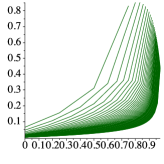
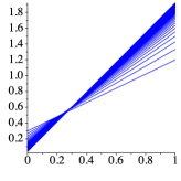
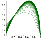
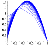
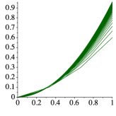
Figure 8: Distributions of the coefficients of polynomials of type $\mathscr{E}\langle\!\langle n+pv+q,-v;1\rangle\!\rangle$ for $n=3,\dots,50$: (from left to right) $(p,q)=(2,-0.5)$, $(2,0)$, $(2,0.5)$, $(2,1)$, $(3,1)$.

8.2 Uniform limit laws again

We saw two occurrences of uniform limit law in the above table (being a special case of beta distribution): A279891 and A123310. Other less trivial examples are the following.

OEIS	Type	OGF	Limit law
A104709	$\mathscr{E}\langle\!\langle 2n+1+v,-(1+v);1\rangle\!\rangle$	$\frac{1}{(1-2z)(1-(1+v)z)}$	Uniform$[0,\frac{1}{2}]$
A193851	$\mathscr{E}\langle\!\langle 3n+1+2v,-(1+2v);1\rangle\!\rangle$	$\frac{1}{(1-3z)(1-(1+2v)z)}$	Uniform$[0,\frac{2}{3}]$
A193861	$\mathscr{E}\langle\!\langle 3n+2+v,-(2+v);1\rangle\!\rangle$	$\frac{1}{(1-3z)(1-(2+v)z)}$	Uniform$[0,\frac{1}{3}]$

Their reciprocal polynomials are of the same form (9) but with quadratic $\alpha(v)$. See Figure 9 for a graphical rendering.

OEIS	Type	Limit law	Recip. of
A054143	$\mathscr{E}\langle\!\langle(1+2v-v^{2})n+v(1+v),-v(1+v);1\rangle\!\rangle$	Uniform$[\frac{1}{2},1]$	A104709
A193850	$\mathscr{E}\langle\!\langle(2+2v-v^{2})n+v(2+v),-v(2+v);1\rangle\!\rangle$	Uniform$[\frac{2}{3},1]$	A193851
A193860	$\mathscr{E}\langle\!\langle(1+4v-2v^{2})n+v(1+2v),-v(1+2v);1\rangle\!\rangle$	Uniform$[\frac{1}{3},1]$	A193861

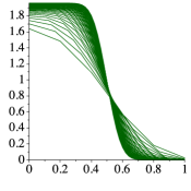
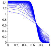
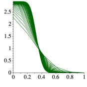
A104709	A193851	A193861

Figure 9: The histograms corresponding to A104709, A193851 and A193861.

Other Eulerian recurrences not of the form (102) but with a uniform limit law include

A118175	$P_{n}(v)=\sum_{1\leqslant j\leqslant 2n}v^{j}$	$P_{n}\in\mathscr{E}\langle\!\langle\frac{v(2-v)n-v(1-2v)}{n},-\frac{v^{2}}{n};1\rangle\!\rangle$	Uniform$[0,1]$
A071028	$P_{n}(v)=\sum_{0\leqslant j\leqslant n}v^{2j}$	$P_{n}\in\mathscr{E}\langle\!\langle\frac{n+v^{2}}{n},-\frac{v(1+v)}{2n};1\rangle\!\rangle$	Uniform$[0,1]$

Note that a very similar-looking EGF $\frac{1}{(1-z)(1-(1+2v)z)}$, which is A193862 (reciprocal of A115068, enumerating elements in Coxeter group with certain descent sets), leads to the CLT $\mathscr{N}\bigl{(}{\frac{2}{3}n,\frac{2}{9}n}\bigr{)}$, although both sequences do not satisfy the recurrence (9). This follows from a direct calculation.

8.3 Rayleigh and half-normal limit laws ($\frac{\beta}{\alpha}=-\frac{1}{2}$)

We consider here $\tau_{1}=\frac{1}{2}$ for which many different limit laws are possible. For example, the polynomials with

$$P_{n}\in\mathscr{E}\langle\!\langle 2n-2+v,-v;1+v\rangle\!\rangle,$$

contain only nonnegative coefficients, and follow a limit law with the density $\frac{1}{8}x^{3}e^{-\frac{1}{4}x^{2}}$. This is proved directly from (97). Similarly, the polynomials $P_{n}\in\mathscr{E}\langle\!\langle 2n+bv,-v;1\rangle\!\rangle$ leads to the limit law with the density

$$\frac{b2^{-b}}{\Gamma\bigl{(}{\frac{1}{2}(b+1)}\bigr{)}}\,x^{b-1}\int_{x}^{\infty}e^{-\frac{1}{4}t^{2}}\,\mathrm{d}{t}\qquad(b>0;x>0).$$

Instead of describing all possible limit laws for which we have few applications, we address the following question, based on the examples we collected: under which conditions will the limit law of the coefficients be either Rayleigh or half-normal (two of the most common non-normal laws in lattice paths, random trees, random mappings, etc.)? For more instances and techniques for these two laws, see [79, 236] and the references therein. It turns out that these are very special laws from our framework and very strong restrictions are needed. We give a complete characterization of this question.

Recall that the Rayleigh and half-normal distributions with scale $\sigma>0$ (which corresponds to the mode of the distribution) have the densities

$$\frac{x}{\sigma^{2}}\,e^{-\frac{x^{2}}{2\sigma^{2}}}\quad\text{and}\quad\frac{\sqrt{2}}{\sqrt{\pi}\,\sigma}\,e^{-\frac{x^{2}}{2\sigma^{2}}}\qquad(x\geqslant 0),$$

respectively. While the Taylor expansion of the former contains only odd powers, that of the latter contains only even powers. The corresponding $m$th moments have the forms

$$\sqrt{\pi}\frac{\Gamma(m+1)}{\Gamma\bigl{(}{\frac{m}{2}+\frac{1}{2}}\bigr{)}}\,\left(\frac{\sigma}{\sqrt{2}}\right)^{m}\quad\text{and}\quad\frac{\Gamma(m+1)}{\Gamma\bigl{(}{\frac{m}{2}+1}\bigr{)}}\,\left(\frac{\sigma}{\sqrt{2}}\right)^{m},$$ (104)

respectively.

8.3.1 Characterizations of Rayleigh and half-normal limit laws

To describe our characterization of the two special limit laws, we define the function

$$\mathscr{F}_{\alpha}(p,q,\rho;z):=(1-\alpha z)^{-p}\bigl{(}{\bigl{(}{1-\rho(1-v)}\bigr{)}\sqrt{1-\alpha z}+\rho(1-v)}\bigr{)}^{-q},$$

which equals $\alpha^{q}$ times $F$ in (90) when $\beta=-\frac{1}{2}\alpha$, $\beta^{\prime}=-\frac{1}{2}\rho$, $\gamma=\alpha\bigl{(}{p-1+\frac{1}{2}q}\bigr{)}$, $\gamma^{\prime}=\frac{1}{2}q\rho$, $c_{0}=1$ and $c_{1}=0$. For our uses, we need the following conditions for the nonnegativity of the coefficients $[v^{k}z^{n}]\mathscr{F}_{\alpha}$.

Lemma 9.

Let $P_{n}(v):=[z^{n}]\mathscr{F}_{\alpha}(p,q,\rho;z)$. Assume $\alpha>0$. (i) If $p=0$ and $q>0$, then $[v^{k}]P_{n}(v)\geqslant 0$ for all $n,k\geqslant 0$ iff $0\leqslant\rho\leqslant 1$; and (ii) if $p\geqslant\frac{1}{2}$ and $0<q\leqslant 2$, then $[v^{k}]P_{n}(v)\geqslant 0$ for all $n,k\geqslant 0$ iff $0\leqslant\rho\leqslant\frac{3}{2}$.

Proof.

Assume without loss of generality $\alpha=1$. Consider first the case when $p=0$ and $q>0$:

$$P_{n}(v)=[z^{n}]\bigl{(}{\bigl{(}{1+\rho(v-1)}\bigr{)}\sqrt{1-z}-\rho(v-1)}\bigr{)}^{-q}=:[z^{n}](1-g(z))^{-q},$$

where $g(z):=\tilde{\rho}(v)(1-\sqrt{1-z})$ with $\tilde{\rho}(v):=1+\rho(v-1)$. Then

$$g=z\,\frac{\tilde{\rho}(v)^{2}}{2\tilde{\rho}(v)-g}.$$

By Lagrange inversion formula [224]

$$P_{n}(v) =[z^{n}](1-g(z))^{-q}=\frac{q}{n}[t^{n-1}]\frac{1}{(1-t)^{q+1}}\left(\frac{\tilde{\rho}(v)^{2}}{2\tilde{\rho}(v)-t}\right)^{n}$$

$$=\frac{q}{n}\sum_{1\leqslant j\leqslant n}\binom{2n-1-j}{n-1}\binom{q+j-1}{q}\frac{\tilde{\rho}(v)^{j}}{2^{2n-j}}.$$ (105)

Then

$$[v^{k}]P_{n}(v)=\frac{q}{n}\,\rho^{k}\sum_{k\leqslant j\leqslant n}\binom{2n-1-j}{n-1}\binom{q+j-1}{q}\binom{j}{k}\frac{(1-\rho)^{j-k}}{2^{2n-j}}.$$ (106)

If $0\leqslant\rho\leqslant 1$, then all coefficients are nonnegative and we obtain $[v^{k}]P_{n}(v)\geqslant 0$. On the other hand, since $P_{1}(v)=\frac{1}{2}q((1-\rho)+\rho v)$, we see that if $[v^{k}]P_{n}(v)\geqslant 0$ for $k,n\geqslant 0$, then $\rho\in[0,1]$. This proves the necessity.

For the second case $p\geqslant\frac{1}{2}$ and $0<q\leqslant 2$, writing $\rho=1+t$ and $Z:=1-\sqrt{1-z}$, we have

$$[v^{k}]P_{n}(v) =[z^{n}](1-z)^{-p}[v^{k}](1+tZ-(1+t)vZ)^{-q}$$

$$=\binom{q+k-1}{k}(1+t)^{k}[z^{n}]Z^{k}(1-Z)^{-2p}(1+tZ)^{-q-k}.$$

By using the relation $Z(2-Z)=z$, applying Lagrange inversion formula and then changing the variables $Z\mapsto 2w$, we obtain

$$[z^{n}]Z^{k}(1-Z)^{-2p}(1+tZ)^{-q-k}$$

$$\qquad=2^{k-2n}[w^{n-k}](1-2w)^{1-2p}(1+2tw)^{-q-k}(1-w)^{-n-1}$$

$$\qquad=2^{k-2n}[w^{n-k}](1-2w)^{1-2p}\left((1+2tw)(1-w)\right)^{-q-k}(1-w)^{-n-1+q+k}.$$

Since $p\geqslant\frac{1}{2}$, we see that $[w^{j}](1-w)^{1-2p}\geqslant 0$ for all $j\geqslant 0$; on the other hand, since $0<q\leqslant 2$, we have $n+1-q-k\geqslant 0$ for $0\leqslant k\leqslant n-1$, implying that $[w^{j}](1-w)^{-n-1+q+k}\geqslant 0$ for $j\geqslant 0$ and $0\leqslant k\leqslant n-1$; also $[v^{n}]P_{n}(v)=\binom{q+n-1}{n}(1+t)^{-q}2^{-n}$ is always nonnegative. Furthermore, for $0\leqslant k\leqslant n$, if $1-2t\geqslant 0$, then

$$[w^{j}]\left((1+2tw)(1-w)\right)^{-q-k}\geqslant 0\text{ for }j\geqslant 0.$$

For the necessity, we observe first that $[v]P_{1}(v)=\frac{1}{2}q\rho<0$ if $\rho<0$; also

$$[v^{n-1}]P_{n}(v)=\binom{q+n-2}{n-1}(1+t)^{n-1}2^{-n-1}((1-2t)n+O(1)),$$

which becomes negative if $t>\frac{1}{2}$ or $\rho>\frac{3}{2}$ for large enough $n$. This implies the necessity of $0\leqslant\rho\leqslant\frac{3}{2}$. ∎

Theorem 7.

Assume that $P_{n}(v)$ satisfies the recurrence (82) with $\tau_{1}=\frac{1}{2}$ and $\beta^{\prime}<0$. Let $\sigma:=-\frac{2\sqrt{2}\beta^{\prime}}{\alpha}$. Then the coefficients of the polynomials $\mathbb{E}(v^{X_{n}}):=\frac{P_{n}(v)}{P_{n}(1)}$ are asymptotically Rayleigh distributed

$$\frac{X_{n}}{\sigma\sqrt{n}}\stackrel{{\scriptstyle d}}{{\longrightarrow}}X,$$

where $X$ has the density $xe^{-\frac{1}{2}x^{2}}$ for $x\geqslant 0$ iff the EGF $F$ of $P_{n}$ has one of the following five forms: $F\in\{\mathcal{R}_{1},\dots,\mathcal{R}_{5}\}$, where

$$\mathcal{R}_{1}(z) :=(c_{0}+c_{1}(v-1))\mathscr{F}_{\alpha}\bigl{(}{0,1,\tfrac{c_{1}}{c_{0}};z}\bigr{)},$$

$$\mathcal{R}_{2}(z) :=c_{0}\mathscr{F}_{\alpha}\bigl{(}{0,1,-\tfrac{2\beta^{\prime}}{\alpha};z}\bigr{)}\quad\text{with}\;-\tfrac{1}{2}\alpha\leqslant\beta^{\prime}<0,$$

$$\mathcal{R}_{3}(z) :=(c_{0}+c_{1}(v-1))\mathscr{F}_{\alpha}\bigl{(}{\tfrac{1}{2},2,\tfrac{c_{1}}{c_{0}};z}\bigr{)},$$

$$\mathcal{R}_{4}(z) :=c_{0}\mathscr{F}_{\alpha}\bigl{(}{\tfrac{1}{2},2,-\tfrac{2\beta^{\prime}}{\alpha};z}\bigr{)}\quad\text{with}\;-\tfrac{3}{4}\alpha\leqslant\beta^{\prime}<0,$$

$$\mathcal{R}_{5}(z) :=c_{0}\mathscr{F}_{\alpha}\bigl{(}{\tfrac{3}{2},2,\tfrac{3c_{1}}{2c_{0}};z}\bigr{)}+c_{1}(v-1)\mathscr{F}_{\alpha}\bigl{(}{\tfrac{3}{2},3,\tfrac{3c_{1}}{2c_{0}};z}\bigr{)}.$$

On the other hand, the sequence of random variables $\{X_{n}\}$ is asymptotically half-normally distributed

$$\frac{X_{n}}{\sigma\sqrt{n}}\stackrel{{\scriptstyle d}}{{\longrightarrow}}Y,$$

where $Y$ has the density $\sqrt{\frac{2}{\pi}}\,e^{-\frac{1}{2}x^{2}}$ for $x\geqslant 0$ iff the EGF of $P_{n}$ has one of the following three forms: $F\in\{\mathcal{H}_{1},\mathcal{H}_{2},\mathcal{H}_{3}\}$, where

$$\mathcal{H}_{1}(z) :=(c_{0}+c_{1}(v-1))\mathscr{F}_{\alpha}\bigl{(}{\tfrac{1}{2},1,\tfrac{c_{1}}{c_{0}};z}\bigr{)},$$

$$\mathcal{H}_{2}(z) :=c_{0}\mathscr{F}_{\alpha}\bigl{(}{\tfrac{1}{2},1,-\tfrac{2\beta^{\prime}}{\alpha};z}\bigr{)}\quad\text{with}\;-\tfrac{3}{4}\alpha\leqslant\beta^{\prime}<0,$$

$$\mathcal{H}_{3}(z) :=(c_{0}+c_{1}(v-1))\mathscr{F}_{\alpha}\bigl{(}{\tfrac{3}{2},2,\tfrac{c_{1}}{c_{0}};z}\bigr{)}.$$

We see that in either case the seven parameters in (82) are now reduced to only three (including $\alpha$) as far as the two limit laws are concerned. Also the coefficients of $\mathcal{R}_{1},\mathcal{R}_{3},\mathcal{R}_{5},\mathcal{H}_{1},\mathcal{H}_{3}$ are always nonnegative since $0\leqslant\frac{c_{1}}{c_{0}}\leqslant 1$, but for $\mathcal{R}_{2},\mathcal{R}_{4},\mathcal{H}_{2}$ one needs further restrictions on $\beta^{\prime}$ using Lemma 9.

Proof.

Consider first the Rayleigh limit law. Since $\tau_{1}=\frac{1}{2}$, we have, by Proposition 4,

$$\mathbb{E}\left(\frac{X_{n}}{\sigma\sqrt{n}}\right)^{m}\sim\tilde{K}_{m},\;\text{where}\;\tilde{K}_{m}=\frac{\Gamma\bigl{(}{m+\tau_{3}}\bigr{)}\Gamma(\tau_{2}+1)(\rho_{1}m+\tau_{3})}{\Gamma\bigl{(}{\tau_{3}+1}\bigr{)}\Gamma\bigl{(}{\frac{m}{2}+1+\tau_{2}}\bigr{)}2^{\frac{m}{2}}}.$$ (107)

Here $\sigma:=-\frac{2\sqrt{2}\beta^{\prime}}{\alpha}$ and $\rho_{1}:=-\frac{c_{1}\alpha}{2c_{0}\beta^{\prime}}$. By equating $\tilde{K}_{m}$ to the moments (104) of the Rayleigh distribution, we are led to the identity for all $m\geqslant 0$

$$\tilde{K}_{m}=\frac{\Gamma\bigl{(}{m+\tau_{3}}\bigr{)}\Gamma(\tau_{2}+1)(\rho_{1}m+\tau_{3})}{\Gamma\bigl{(}{\tau_{3}+1}\bigr{)}\Gamma\bigl{(}{\frac{m}{2}+1+\tau_{2}}\bigr{)}2^{\frac{m}{2}}}=\sqrt{\pi}\frac{\Gamma(m+1)}{\Gamma\bigl{(}{\frac{m}{2}+\frac{1}{2}}\bigr{)}2^{\frac{m}{2}}}.$$ (108)

If $c_{1}=0$, then $\rho_{1}=0$ and the above identity becomes

$$\tilde{K}_{m}=\frac{\tau_{3}\Gamma\bigl{(}{m+\tau_{3}}\bigr{)}\Gamma(\tau_{2}+1)}{\Gamma\bigl{(}{\tau_{3}+1}\bigr{)}\Gamma\bigl{(}{\frac{m}{2}+1+\tau_{2}}\bigr{)}2^{\frac{m}{2}}}=\sqrt{\pi}\frac{\Gamma(m+1)}{\Gamma\bigl{(}{\frac{m}{2}+\frac{1}{2}}\bigr{)}2^{\frac{m}{2}}}.$$

Since this holds for $m\geqslant 0$ (including $m\to\infty$), we see that, by Stirling’s formula,

$$\frac{\tilde{K}_{m}}{\bigl{(}{\frac{m}{e}}\bigr{)}^{\frac{m}{2}}}=\frac{\tau_{3}\Gamma(\tau_{2}+1)}{\Gamma(\tau_{3}+1)}\,m^{\tau_{3}-\tau_{2}-1}2^{\tau_{2}+\frac{1}{2}}(1+o(1)),$$

for large $m$, while for the Rayleigh moments

$$\frac{\sqrt{\pi}\Gamma(m+1)}{\Gamma\bigl{(}{\frac{m}{2}+\frac{1}{2}}\bigr{)}\bigl{(}{\frac{2}{e}m}\bigr{)}^{\frac{m}{2}}}=\sqrt{\pi m}(1+o(1)).$$

It follows that $\tau_{3}=\frac{3}{2}+\tau_{2}$. Substituting this into (108) with $m=2$, and then solving for $\tau_{2}$, we obtain two solutions: $\tau_{2}=\pm\frac{1}{2}$. If $\tau_{2}=-\frac{1}{2}$, then $\tau_{3}=1$, and $P_{n}$ has the pattern

$$P_{n}\in\mathscr{E}\langle\!\langle\alpha n-\tfrac{1}{2}\alpha-\beta^{\prime}(v-1),-\tfrac{1}{2}\alpha+\beta^{\prime}(v-1);c_{0}\rangle\!\rangle,$$

which implies that the EGF equals $\mathcal{R}_{2}$ by (90).

On the other hand, if $\tau_{2}=\frac{1}{2}$, then $\tau_{3}=2$, and $P_{n}$ satisfies

$$P_{n}\in\mathscr{E}\langle\!\langle\alpha n+\tfrac{1}{2}\alpha-2\beta^{\prime}(v-1),-\tfrac{1}{2}\alpha+\beta^{\prime}(v-1);c_{0}\rangle\!\rangle,$$

so that $F=\mathcal{R}_{4}$. Note that $\mathcal{R}_{2}$ and $\mathcal{R}_{4}$ are connected by a differentiation:

$$\partial_{z}\mathscr{F}_{\alpha}(0,1,\rho;z)=\tfrac{1}{2}\alpha(1+\rho(v-1))\mathscr{F}_{\alpha}\bigl{(}{\tfrac{1}{2},2,\rho;z}\bigr{)}.$$ (109)

Assume now $c_{1}>0$. Then $\rho_{1}>0$ and

$$\frac{\tilde{K}_{m}}{\bigl{(}{\frac{m}{e}}\bigr{)}^{\frac{m}{2}}}=\rho_{1}\frac{\Gamma(\tau_{2}+1)}{\Gamma(\tau_{3}+1)}\,m^{\tau_{3}-\tau_{2}}2^{\tau_{2}+\frac{1}{2}}(1+o(1)),$$

for large $m$, implying that $\tau_{3}=\frac{1}{2}+\tau_{2}$. Substituting this into (108) with $m=2,4$ and then solving for $\rho_{1}$ and $\tau_{2}$, we get three feasible solutions:

$$(\rho_{1},\tau_{2})=\bigl{\{}\bigl{(}{1,-\tfrac{1}{2}}\bigr{)},\bigl{(}{1,\tfrac{1}{2}}\bigr{)},\bigl{(}{\tfrac{2}{3},\tfrac{3}{2}}\bigr{)}\bigr{\}},$$

leading to the three patterns

$$P_{n}\in\begin{cases}\mathscr{E}\langle\!\langle\alpha n-\tfrac{1}{2}\alpha,-\tfrac{1}{2}\alpha-\tfrac{c_{1}\alpha}{2c_{0}}(v-1);c_{0}+c_{1}(v-1)\rangle\!\rangle,\\ \mathscr{E}\langle\!\langle\alpha n+\tfrac{1}{2}\alpha+\tfrac{c_{1}\alpha}{2c_{0}}(v-1),-\tfrac{1}{2}\alpha-\tfrac{c_{1}\alpha}{2c_{0}}(v-1);c_{0}+c_{1}(v-1)\rangle\!\rangle,\\ \mathscr{E}\langle\!\langle\alpha n+\tfrac{3}{2}\alpha+\tfrac{3c_{1}\alpha}{2c_{0}}(v-1),-\tfrac{1}{2}\alpha-\tfrac{3c_{1}\alpha}{4c_{0}}(v-1);c_{0}+c_{1}(v-1)\rangle\!\rangle,\end{cases}$$

respectively in sequential order. These correspond to $\mathcal{R}_{1}$, $\mathcal{R}_{3}$ and $\mathcal{R}_{5}$, respectively. Note that $\sigma=\frac{\sqrt{2}c_{1}}{c_{0}}$ in the cases of $\mathcal{R}_{1}$ and $\mathcal{R}_{3}$, and $\sigma=\frac{3c_{1}}{\sqrt{2}c_{0}}$ in the other case, so that $\sigma$ equals $\sqrt{2}$ times the third parameter of the function $\mathscr{F}_{\alpha}$ in all cases $\mathcal{R}_{1},\dots,\mathcal{R}_{5}$. Also $\mathcal{R}_{1}$, $\mathcal{R}_{3}$ and $\mathcal{R}_{5}$ are essentially connected by successive derivatives (up to change of parameters and multiplicative factors) by the relations (109) and

$$\partial_{z}\mathscr{F}_{\alpha}\bigl{(}{\tfrac{1}{2},2,\rho;z}\bigr{)}=\tfrac{3}{2}\alpha\mathscr{F}_{\alpha}\bigl{(}{\tfrac{3}{2},2,\rho;z}\bigr{)}+\alpha\rho(v-1)\mathscr{F}_{\alpha}\bigl{(}{\tfrac{3}{2},3,\rho;z}\bigr{)}.$$

The proof for half-normal limit law is similar, starting from the asymptotic estimate

$$\frac{\Gamma(m+1)}{\Gamma\bigl{(}{\frac{m}{2}+1}\bigr{)}\bigl{(}{\frac{2}{e}m}\bigr{)}^{\frac{m}{2}}}=\sqrt{2}(1+o(1)),$$

implying either $\rho_{1}=0,\tau_{3}=1+\tau_{2}$ or $\rho_{1}>0,\tau_{3}=\tau_{2}$. By the same arguments used above, we then obtain $\tau_{2}=0$ in the former case, and $(\rho_{1},\tau_{2})=(1,0)$ or $\bigl{(}{\frac{1}{2},1}\bigr{)}$ in the latter case, yielding the three patterns

$$P_{n}\in\begin{cases}\mathscr{E}\langle\!\langle\alpha n-\beta^{\prime}(v-1),-\tfrac{1}{2}\alpha+\beta^{\prime}(v-1);c_{0}\rangle\!\rangle,\\ \mathscr{E}\langle\!\langle\alpha n,-\tfrac{1}{2}\alpha-\tfrac{c_{1}}{2c_{0}}\alpha(v-1);c_{0}+c_{1}(v-1)\rangle\!\rangle,\\ \mathscr{E}\langle\!\langle\alpha n+\alpha+\tfrac{c_{1}}{c_{0}}\alpha(v-1),-\tfrac{1}{2}\alpha-\tfrac{c_{1}}{c_{0}}\alpha(v-1);c_{0}+c_{1}(v-1)\rangle\!\rangle,\end{cases}$$

corresponding to $\mathcal{H}_{2}$, $\mathcal{H}_{1}$, and $\mathcal{H}_{3}$, respectively. ∎

Another interesting property of $X_{n}$ is that the difference polynomials $\Delta_{n}(v):=P_{n}(v)-P_{n-1}(v)$ have only positive coefficients and the same limit law as that for $P_{n}(v)$.

Corollary 8.

Assume that $P_{n}(v)$ is as in Theorem 7, $[v^{k}]\Delta_{n}(v)\geqslant 0$ and $\mathbb{E}\bigl{(}{v^{Z_{n}}}\bigr{)}:=\frac{\Delta_{n}(v)}{\Delta_{n}(1)}$. Then $X_{n}$ and $Z_{n}$ follow the same limit laws.

The result holds in more general settings but we content ourselves with the current formulation due to limited applications.

Proof.

By Proposition 4, we see that

$$P_{n}^{(m)}(1)\sim P_{n}(1)K_{m}n^{m\tau_{1}}\qquad(m\geqslant 0),$$

and the corollary follows from the relation $P_{n}(1)=(\alpha n+\gamma)P_{n-1}(1)$. ∎

8.3.2 Examples. I. Rayleigh laws

Consider the Catalan triangle A039598:

$$P_{n}(v):=\sum_{0\leqslant k\leqslant n}\frac{2(k+1)}{n+k+2}\binom{2n+1}{n-k}v^{k},$$

which has a large number of combinatorial interpretations such as the number of leaves at level $k+1$ in ordered trees with $n+1$ edges. This sequence of polynomials satisfies the recurrence

$$P_{n}\in\mathscr{E}\left\langle\!\left\langle\frac{4n+2v}{n+1},-\frac{1+v}{n+1};1\right\rangle\!\right\rangle.$$ (110)

The EGF of $(n+1)!P_{n}(v)$ is of type $\mathcal{R}_{4}$ (with $c_{1}=0$ and $\frac{\gamma}{\alpha}=\frac{1}{2}$) and equals $\mathscr{F}_{4}\bigl{(}{\frac{1}{2},2,\frac{1}{2};z}\bigr{)}$, which, by an integration, gives

$$\sum_{n\geqslant 0}P_{n}(v)z^{n+1}=\frac{1-\sqrt{1-4z}}{(1+v)\sqrt{1-4z}+1-v}.$$

By Theorem 7, we see that the limit law of the coefficients is Rayleigh with $\sigma=\frac{1}{2}$, which also follows from the closed-form expression; see Figure 10. Stronger asymptotic approximations and local limit theorems can also be derived.

This sequence has many minor variants that do not change the Rayleigh limit distribution of the coefficients; for example (the case A122919 following from Corollary 8):

A039598	$:=$	$P_{n}(v)$	Rayleigh$\bigl{(}{\frac{1}{\sqrt{2}}}\bigr{)}$
A039599	$=$	$\frac{vP_{n}(v)+P_{n-1}(0)}{1+v}=:R_{n}(v)$	Rayleigh$\bigl{(}{\frac{1}{\sqrt{2}}}\bigr{)}$
A050166	$=$	Reciprocal of $P_{n}(v)$	$\text{Rayleigh}\bigl{(}{\frac{1}{\sqrt{2}}}\bigr{)}$
A122919	$=$	$P_{n}(v)-P_{n-1}(v)$	Rayleigh$\bigl{(}{\frac{1}{\sqrt{2}}}\bigr{)}$
A128899	$=$	$vP_{n-1}(v)$	Rayleigh$\bigl{(}{\frac{1}{\sqrt{2}}}\bigr{)}$
A118920	$=$	$2P_{n}(v)$	Rayleigh$\bigl{(}{\frac{1}{\sqrt{2}}}\bigr{)}$
A053121	$=$	$\left\{\begin{array}[]{ll}vP_{\lfloor\frac{1}{2}n\rfloor}(v^{2}),&n\text{ odd}\\ R_{\frac{1}{2}n}(v^{2}),&n\text{ even}\end{array}\right.$	Rayleigh$\bigl{(}{\frac{1}{\sqrt{2}}}\bigr{)}$

Some other OEIS sequences leading to Rayleigh limit laws are listed in the following table (using the format (100)).

OEIS	Type	$[v^{k}]P_{n}(v)$	Limit law
A039599	$\mathscr{E}\langle\!\langle\frac{4n+v-3}{n},-\frac{1+v}{n};1\rangle\!\rangle$	$\frac{2k+1}{n+k+1}\binom{2n}{n-k}$	Rayleigh$\bigl{(}{\frac{1}{\sqrt{2}}}\bigr{)}$
A102625	$\mathscr{E}\langle\!\langle 2n+v,-v;v\rangle\!\rangle$	$\frac{k(2n-k+1)!}{(n-k+1)!2^{n-k+1}}$	Rayleigh$\bigl{(}{\sqrt{2}}\bigr{)}$
A108747	$\mathscr{E}\langle\!\langle\frac{4n+2v}{n+1},-\frac{2v}{n+1};2v\rangle\!\rangle$	$\frac{k2^{k}}{2n+2-k}\binom{2n+2-k}{n+1}$	Rayleigh$\bigl{(}{\sqrt{2}}\bigr{)}$

Their reciprocal polynomials also follow the same Rayleigh limit laws.

Recip. of	OEIS	Type	Limit law
A039599	A050165	$\mathscr{E}\langle\!\langle\frac{(1+4v-v^{2})n-3v+v^{2}}{n},-\frac{v(1+v)}{n};1\rangle\!\rangle$	Rayleigh$\bigl{(}{\frac{1}{\sqrt{2}}}\bigr{)}$
A102625	A193561	$\mathscr{E}\langle\!\langle(1+v)n+1,-v;1\rangle\!\rangle$	Rayleigh$\bigl{(}{\sqrt{2}}\bigr{)}$
A039598	A050166	$\mathscr{E}\langle\!\langle\frac{(1+4v-v^{2})n+1+v^{2}}{n+1},-\frac{v(1+v)}{n+1};1\rangle\!\rangle$	Rayleigh$\bigl{(}{\frac{1}{\sqrt{2}}}\bigr{)}$

Among these OEIS sequences, A102625 was one of our motivating examples of non-normal limit laws (see Figure 10), and has many combinatorial interpretations such as the root degree of plane-oriented recursive trees and the waiting time in a memory game; see [1, 15, 171] and OEIS A102625 page for more information.

Yet another occurrence of A102625 and Rayleigh limit law is as follows. Consider the Catalan triangle A009766 (or ballot numbers):

$$R_{n}(v):=\sum_{0\leqslant k\leqslant n}\frac{n-k+1}{n+1}\binom{n+k}{k}v^{k}.$$

Then $R_{n}(v)$ satisfies the recurrence

$$(n+1)R_{n}(v)=((1+2v)n+1)R_{n-1}(v)-v(1-2v)R_{n-1}^{\prime}(v)\qquad(n\geqslant 1),$$

with $R_{0}(v)=1$. The distribution of the coefficients is negative binomial with parameters $2$ and $\frac{1}{2}$. Also they are related to $P_{n}(v)$ of A102625 by $P_{n+1}(v)=v^{n+2}R_{n}\bigl{(}{\frac{1}{2v}}\bigr{)}$.

These sequences are rather simple in nature as they all have a neat closed-form expression for the coefficients. Less trivial examples can be generated by using (105) with $\rho\in\bigl{(}{0,\frac{1}{2}}\bigr{)}$, say.

8.3.3 Examples. II. Half-normal laws

Consider sequence A193229:

$$P_{n}(v)=\sum_{0\leqslant k\leqslant n}\frac{(2n-k)!}{(n-k)!2^{n-k}}\,v^{k};$$

see [171] for a characterization via grammars. Then $P_{n}$ satisfies $\mathscr{E}\langle\!\langle 2n-1+v,-v;1\rangle\!\rangle$, which is of type $\mathcal{H}_{2}$, and we get a half-normal limit law for the coefficients; see Figure 10. Note that a conjecture mentioned on the OEIS webpage for A193229 can be easily proved, stating that $[v^{k}]P_{n}(v)$ is equal to the $(k+1)$st term in the top row of $M^{n}$, where $M=(m_{i,j})$ with $m_{i,j}=i$ for $1\leqslant j\leqslant i+1$ and $i=0$ for $j\geqslant i+2$.

An essentially identical sequence connected to Banach’s matchbox problem is A164705, which can be generated by $P_{n}\in\mathscr{E}\langle\!\langle 4,-\frac{2v}{n};\tfrac{1}{2}v\rangle\!\rangle$ and has the closed-form expression $\binom{2n-k}{n}2^{k-1}$. The EGF is then of type $\mathcal{H}_{1}$, and we get the same half-normal limit law.

Interestingly, the sequence A001497, which corresponds to Bessel polynomials, differs from A193229 by a factor of $k!$, namely, the EGF equals

$$\frac{e^{v(1-\sqrt{1-2z})}}{\sqrt{1-2z}},$$

whose coefficients lead to a Poisson$(1)$ limit law.

Another instance is A111418 (right-hand side of odd-numbered rows of Pascal’s triangle): $[v^{k}]P_{n}(v)=\binom{2n+1}{n-k}$, and $P_{n}$ satisfies $P_{n}\in\mathscr{E}\langle\!\langle\frac{4n-1+v}{n},-\frac{1+v}{n};1\rangle\!\rangle,$ again of type $\mathcal{H}_{1}$, so that the coefficients lead to a half-normal limit law; see Figure 10. The reciprocal polynomial of $P_{n}$ corresponds to sequence A122366, which satisfies $Q_{n}\in\mathscr{E}\langle\!\langle\frac{(1+4v-v^{2})n-v(1-v)}{n},-\frac{v(1+v)}{n};1\rangle\!\rangle;$ compare with the normal examples in Section 5.5.3. A signed version of A111418 is A113187: $R_{n}\in\mathscr{E}\langle\!\langle-\frac{4n-1+v}{n},-\frac{1+v}{n};1\rangle\!\rangle.$ We have $(-1)^{n}R_{n}(-v)=P_{n}(v)$, and we get the same half-normal limit law for the absolute values of the coefficients.

These examples are summarized in the following table.

OEIS	Type	$[v^{k}]P_{n}(v)$	Limit law
A193229	$\mathscr{E}\langle\!\langle 2n+v-1,-v;1\rangle\!\rangle$	$\frac{(2n-k)!}{(n-k)!2^{n-k}}$	Half-Normal$\bigl{(}{\sqrt{2}}\bigr{)}$
A164705	$\mathscr{E}\langle\!\langle 4,-\frac{2v}{n};\frac{1}{2}v\rangle\!\rangle$	$\binom{2n-k}{n}2^{k-1}$	Half-Normal$\bigl{(}{\sqrt{2}}\bigr{)}$
$\begin{array}[]{l}\text{\href https://oeis.org/A111418}\\ |\text{\href https://oeis.org/A113187}|\end{array}$	$\mathscr{E}\langle\!\langle\frac{4n+v-1}{n},-\frac{1+v}{n};1\rangle\!\rangle$	$\binom{2n+1}{n-k}$	Half-Normal$\bigl{(}{\frac{1}{\sqrt{2}}}\bigr{)}$
A122366	$\mathscr{E}\langle\!\langle\frac{(1+4v-v^{2})n-v(1-v)}{n},-\frac{v(1+v)}{n};1\rangle\!\rangle$	$\binom{2n+1}{k}$	Half-Normal$\bigl{(}{\frac{1}{\sqrt{2}}}\bigr{)}$

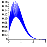
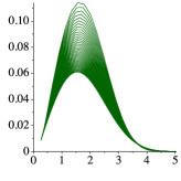
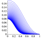
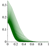
A039598	A102625	A193229	A111418

Figure 10: Rayleigh and half-normal limit laws: the two left histograms for $n=20,\dots,60$ and plotted against $\sqrt{n}$; the two right histograms for $n=10,\dots,50$ and plotted against $n$.

8.4 Other limit laws

We discuss other limit laws based on the recurrence (82) in this subsection.

8.4.1 Mittag-Leffler limit laws

Consider A202550, which is defined by (with a shift of index)

$$[v^{k}]P_{n}(v):=[z^{n+1}]\left(\frac{1-(1-8z)^{\frac{1}{4}}}{1+(1-8z)^{\frac{1}{4}}}\right)^{k+1}\qquad(0\leqslant k\leqslant n).$$

Then $P_{n}(v)$ satisfies the recurrence

$$P_{n}\in\mathscr{E}\left\langle\!\left\langle\frac{8n+2v}{n+1},-\frac{1+v}{n+1};1\right\rangle\!\right\rangle.$$ (111)

By Proposition 4, we see that the $m$th moment of $X_{n}$ is asymptotic to

$$\frac{\Gamma(\tfrac{1}{4})\Gamma(m+1)}{2^{m}\Gamma\bigl{(}{\frac{m}{4}+\frac{1}{4}}\bigr{)}}\qquad(m\geqslant 0),$$

and thus the limit law of the coefficients is a Mittag-Leffler distribution (with the moment generating function (95) with $r=1$) with $p=q=\frac{1}{4}$.

A202550

$P_{n}\in\mathscr{E}\langle\!\langle\frac{8n+2v}{n+1},-\frac{1+v}{n+1};1\rangle\!\rangle$

Mittag-Leffler limit law

In general, replacing $8$ by $\alpha\geqslant 2$ in (111) guarantees $[v^{k}]P_{n}(v)\geqslant 0$ and leads to the moment sequence

$$\frac{\Gamma\bigl{(}{\frac{2}{\alpha}}\bigr{)}\Gamma(m+1)}{2^{m}\Gamma\bigl{(}{\frac{2}{\alpha}(m+1)}\bigr{)}}\qquad(m\geqslant 0),$$

which yields a Mittag-Leffler distribution when $\alpha>2$. Interestingly, the case $\alpha=2$ gives the binomial coefficients (A007318), namely, $P_{n}(v)=(1+v)^{n}$, and we get a CLT $\mathscr{N}\bigl{(}{\frac{1}{2}n,\frac{1}{4}n}\bigr{)}$ instead of a Mittag-Leffler distribution.

Another example leading to a Mittag-Leffler limit law is to extend the recurrence for A102625 by considering $P_{n}\in\mathscr{E}\langle\!\langle\alpha n-1,-v;v\rangle\!\rangle$, for $\alpha\geqslant 2$. We then deduce, again by Proposition 4, that the limit law is a Mittag-Leffler distribution:

$$\frac{X_{n}}{n^{\frac{1}{q}}}\stackrel{{\scriptstyle d}}{{\longrightarrow}}X_{q},\text{ where\; }\mathbb{E}\bigl{(}{e^{X_{q}s}}\bigr{)}=\sum_{m\geqslant 0}\frac{\Gamma\bigl{(}{1-\frac{1}{q}}\bigr{)}}{\Gamma\bigl{(}{1+\frac{m-1}{q}}\bigr{)}}\,s^{m}.$$

Finally, the limit law for the coefficients of the polynomials $P_{n}\in\mathscr{E}\langle\!\langle\alpha n,-(1+v);1+v\rangle\!\rangle$ with $\alpha>2$ is also a Mittag-Leffler.

8.4.2 A mixture of discrete and continuous laws

An example of a similar pattern to (101) but with a completely different behavior is A139524: $P_{n}\in\mathscr{E}\langle\!\langle 2,-\frac{1+v}{n};4+2v\rangle\!\rangle$. A closed-form expression of $P_{n}$ is

$$P_{n}(v)=2^{n+1}+2(1+v)^{n+1}\qquad(n\geqslant 0).$$

The limit law is a mixture of Dirac (at zero) and a normal: $\mathbb{P}(X_{n}=0)\to\frac{1}{3}$ and

$$\mathbb{P}\left(X_{n}=\Bigl{\lfloor}\frac{n}{2}+\frac{\sqrt{n}}{4}x\Bigr{\rfloor}\right)=\frac{2}{3}\cdot\frac{2e^{-\frac{1}{2}x^{2}}}{\sqrt{2\pi n}}\left(1+O\left(\frac{|x|+|x|^{3}}{\sqrt{n}}\right)\right),$$

uniformly for $x=o(n^{\frac{1}{6}})$.

Another similar example is $P_{n}\in\mathscr{E}\langle\!\langle\frac{n+1}{n},-\frac{v}{n};1+v\rangle\!\rangle$. Then

$$P_{n}(v)=n+1+v+\cdots+v^{n+1}\qquad(n\geqslant 0),$$

and one gets a mixture of Dirac and uniform as the limit law. This sequence of polynomials corresponds to the signless version of A167407. A similar variant is A130296 ($P_{n}(v)=nv+v^{2}+\cdots+v^{n}$ for $n\geqslant 1$), but it satisfies a rather messy recurrence involving $P_{n-1}^{\prime}(v)$ and $P_{n-1}^{\prime\prime}(v)$ and is not Eulerian; its reciprocal is A051340.

9 Extensions

In view of the richness and diversity of Eulerian recurrences, many extensions have been made; here we briefly discuss some of them and examine the extent to which the tools used in this paper applies as far as the limit distribution of the coefficients is concerned. For simplicity, we content ourselves with concrete examples rather than the formulation of general theorems. Some extensions and generalizations will be elaborated elsewhere.

Throughout this section, we denote the Eulerian polynomials by $A_{n}(v):=\sum_{0\leqslant k<n}\genfrac{<}{>}{0.0pt}{}{n}{k}v^{k}$.

9.1 Non-homogeneous recurrence

Eulerian recurrences containing an additional non-homogeneous term of the form

$$P_{n}(v)=(\alpha(v)n+\gamma(v))P_{n-1}(v)+\beta(v)(1-v)P_{n-1}^{\prime}(v)+T_{n}(v)\qquad(n\geqslant 1),$$

with $P_{0}(v)$ and $T_{n}(v)$ given, already appeared in our discussions of Lehmer’s polynomials (47) and in Section 4.5.3 on type $D$ Eulerian numbers.

We discuss here two more examples beginning with A065826, which enumerates the descents in permutations starting with an ascent:

$$P_{n}(v)=(vn-1)P_{n-1}(v)+v(1-v)P_{n-1}^{\prime}(v)+vA_{n}(v)\qquad(n\geqslant 2),$$

with $P_{1}(v)=v$. It is easy to see that

$$P_{n}(v)=\sum_{1\leqslant k\leqslant n}k\genfrac{<}{>}{0.0pt}{}{n}{k-1}v^{k}\qquad(n\geqslant 1),$$

so that the EGF is given by

$$v\frac{\partial}{\partial z}\frac{e^{(1-v)z}-1-(1-v)z}{(1-v)(1-ve^{(1-v)z})}.$$

This implies an optimal CLT $\mathscr{N}\bigl{(}{\frac{1}{2}n,\frac{1}{12}n;n^{-\frac{1}{2}}}\bigr{)}$ by Theorem 2.

The reciprocal polynomial $Q_{n}$ of $P_{n}$, satisfying the recurrence

$$Q_{n}(v)=(vn-2v)Q_{n-1}(v)+v(1-v)Q_{n-1}^{\prime}(v)+vA_{n-1}(v)\qquad(n\geqslant 3),$$

with $Q_{2}(v)=v$, appeared in a context of decoding schemes [217].

On the other hand, the derivative $R_{n}(v)$ ($=$ A142706) of $A_{n}(v)$ also satisfies a similar recurrence

$$R_{n}(v)=(vn+2-3v)R_{n-1}(v)+v(1-v)R_{n-1}^{\prime}(v)+(n-1)A_{n-1}(v)\qquad(n\geqslant 1),$$

with $R_{0}(v)=0$. The same CLT $\mathscr{N}\bigl{(}{\frac{1}{2}n,\frac{1}{12}n;n^{-\frac{1}{2}}}\bigr{)}$ for the coefficients hold.

$v(vA_{n})^{\prime}$	A065826	$\mathscr{N}\bigl{(}{\frac{1}{2}n,\frac{1}{12}n;n^{-\frac{1}{2}}}\bigr{)}$
$A_{n}^{\prime}(v)$	A142706	$\mathscr{N}\bigl{(}{\frac{1}{2}n,\frac{1}{12}n;n^{-\frac{1}{2}}}\bigr{)}$

Another recurrence appears in [64] (in the context of Voronoi cells of lattices):

$$a_{n,k} =ka_{n-1,k}+(n-k+1)a_{n-1,k-1}+k^{3}\genfrac{<}{>}{0.0pt}{}{n-1}{k-1}+(n-k+1)^{3}\genfrac{<}{>}{0.0pt}{}{n-1}{k-2}.$$

If $P_{n}(v):=\sum_{k}a_{n+1,k}v^{k}$, then (not in OEIS)

$$P_{n}(v) =(vn+v)P_{n-1}(v)+v(1-v)P_{n-1}^{\prime}(v)$$

$$\quad+v(n+1)^{3}A_{n}(v)-v(3vn(n+1)-1+v)A_{n-1}^{\prime}(v)$$

$$\quad+3v^{2}(vn+1)A_{n-1}^{\prime\prime}(v)+v^{3}(1-v)A_{n-1}^{\prime\prime\prime}(v),$$

for $n\geqslant 1$ with $P_{0}(v)=v$ (we shift $n$ by one). By a direct use of our method of moments, we can prove the CLT $\mathscr{N}\bigl{(}{\frac{1}{2}n,\frac{1}{12}n}\bigr{)}$.

9.2 Eulerian recurrences involving $P_{n-2}(v)$

Similar to the previous subsection, the framework

$$P_{n}(v)=a_{n}(v)P_{n-1}(v)+b_{n}(v)(1-v)P_{n-1}^{\prime}(v)+c_{n}(v)P_{n-2}(v),$$ (112)

is also manageable by the approaches we use in this paper. We already saw two examples in Section 5.3. We consider more examples here.

Fibonacci-Eulerian polynomials

An example of the above type appeared in [31]:

$$P_{n}(v)=vnP_{n-1}(v)+v(1-v)P_{n-1}^{\prime}(v)+(1-v)^{2}P_{n-2}(v)\qquad(n\geqslant 2),$$

with $P_{0}(v)=1$ and $P_{1}(v)=v$. The polynomial $P_{n}(v)$ is closely connected to Fibonacci polynomials $F_{n}(v)=vF_{n-1}(v)+F_{n-2}(v)$ for $n\geqslant 2$ with $F_{0}(v)=1$ and $F_{1}(v)=v$ by the relations

$$\sum_{k\geqslant 0}F_{n}(k)v^{k}=\frac{P_{n}(v)}{(1-v)^{n+1}}.$$

Note that $P_{2}(v)=1-v+2v^{2}$ (the only polynomial with negative coefficients). This ($P_{n}$) corresponds to A259708. A CLT $\mathscr{N}\bigl{(}{\frac{1}{2}n,\frac{1}{12}n}\bigr{)}$ holds for the coefficients by the method of moments. In terms of Eulerian polynomials, we have (redefining $A_{0}(v):=v^{-1}$)

$$P_{n}(v)=v\sum_{0\leqslant j\leqslant\lfloor\frac{1}{2}n\rfloor}\binom{n-j}{j}(v-1)^{2j}A_{n-2j}(v)\qquad(n\geqslant 1);$$

see [31]. This can alternatively be derived by solving the PDE of second order satisfied by the EGF using Riemann’s method. Note that this expression of $P_{n}$ is itself an asymptotic expansion for large $n$ and finite $v$; in particular,

$$P_{n}(v)=vA_{n}(v)\left(1+O\bigl{(}{n^{-1}}\bigr{)}\right),$$

uniformly for bounded $v$, and the CLT $\mathscr{N}\bigl{(}{\frac{1}{2}n,\frac{1}{12}n;n^{-\frac{1}{2}}}\bigr{)}$ then follows.

On the other hand, the Fibonacci polynomials $F_{n}(v)$ correspond to A168561 (integer compositions into odd parts); see also the Chebyshev polynomials (with signs) A049310 and A053119. Since the OGF of $F_{n}(v)$ is given by $(1-vz-z^{2})^{-1}$, we deduce the CLT $\mathscr{N}\bigl{(}{\frac{1}{\sqrt{5}}n,\frac{4}{5\sqrt{5}}n;n^{-\frac{1}{2}}}\bigr{)}$ for the coefficients of $F_{n}(v)$ by Theorem 2 with $\rho(v)=\frac{1}{2}\bigl{(}{\sqrt{4+v^{2}}-v}\bigr{)}$. Note that $F_{n}$ also satisfies the recurrence

$$2nF_{n}(v)=(n+1)vF_{n-1}(v)+(4+v^{2})F_{n-1}^{\prime}(v)\qquad(n\geqslant 1).$$

The sequence of polynomials corresponding to A102426 satisfies the same recurrence as $F_{n}$ but with different initial conditions; see also A098925, A169803, A011973, and A092865.

A168561	$\frac{1}{1-vz-z^{2}}$	$\mathscr{N}\bigl{(}{\frac{1}{\sqrt{5}}n,\frac{4}{5\sqrt{5}}n;n^{-\frac{1}{2}}}\bigr{)}$
A049310	$\frac{1}{1-vz+z^{2}}$	signed version of A168561
A053119	$\frac{1}{1-z+v^{2}z^{2}}$	reciprocal of A049310
A098925	$\frac{1}{1-vz-vz^{2}}$	$\mathscr{N}\bigl{(}{\bigl{(}{\frac{1}{2}+\frac{\sqrt{5}}{10}}\bigr{)}n,\frac{\sqrt{5}}{25}n;n^{-\frac{1}{2}}}\bigr{)}$
A092865	$\frac{1}{1+vz+vz^{2}}$	signed version of A098925
A011973	$\frac{1}{1-z-vz^{2}}$	$\mathscr{N}\bigl{(}{\bigl{(}{\frac{1}{2}-\frac{\sqrt{5}}{10}}\bigr{)}n,\frac{\sqrt{5}}{25}n;n^{-\frac{1}{2}}}\bigr{)}$
A169803	$\frac{1+vz}{1-z-vz^{2}}$	$\mathscr{N}\bigl{(}{\bigl{(}{\frac{1}{2}-\frac{\sqrt{5}}{10}}\bigr{)}n,\frac{\sqrt{5}}{25}n;n^{-\frac{1}{2}}}\bigr{)}$
A102426	$\frac{z(1+z-z^{2})}{(1-z^{2})^{2}-vz^{2}}$	$\mathscr{N}\bigl{(}{\frac{\sqrt{5}}{10}n,\frac{\sqrt{5}}{25}n;n^{-\frac{1}{2}}}\bigr{)}$

Derangement polynomials

The derangement polynomials in permutations represent another example of (112). They enumerate for example the number of $n$-derangements with $k$ exceedances, and can be defined by (see [23])

$$P_{n}(v)=\sum_{0\leqslant k\leqslant n}\binom{n}{k}(-1)^{n-k}A_{k}(v)\qquad(n\geqslant 0),$$ (113)

which is sequence A046739 and A271697 (see also A168423 for a signed version) and satisfies the recurrence

$$P_{n}(v)=(n-1)vP_{n-1}(v)+v(1-v)P_{n-1}^{\prime}(v)+(n-1)vP_{n-2}(v)\qquad(n\geqslant 2),$$

with $P_{0}(v)=1$ and $P_{1}(v)=0$.

A CLT of the form $\mathscr{N}\bigl{(}{\frac{1}{2}n,\frac{25}{12}n}\bigr{)}$ for the coefficients was given in [60] but the variance coefficient $\frac{25}{12}$ there should be corrected to $\frac{1}{12}$. See also [49] for the same CLT $\mathscr{N}\bigl{(}{\frac{1}{2}n,\frac{1}{12}n}\bigr{)}$ for a type $B$ analogue with the recurrence

$$R_{n}(v)=(2n-1)vR_{n-1}(v)+2v(1-v)R_{n-1}^{\prime}(v)+2(n-1)vR_{n-2}(v)\qquad(n\geqslant 2),$$

with $R_{0}(v)=1$ and $R_{1}(v)=v$. Both proofs rely on the real-rootedness of the polynomials.

In both cases, while it is possible to apply the method of moments, it is simpler to apply Theorem 2 to the EGFs

$$e^{-vz}\frac{1-v}{1-ve^{(1-v)z}},\quad\text{and}\quad e^{-vz}\frac{1-v}{1-ve^{2(1-v)z}},$$

respectively, yielding the stronger result $\mathscr{N}\bigl{(}{\frac{1}{2}n,\frac{1}{12}n;n^{-\frac{1}{2}}}\bigr{)}$.

Binomial-Eulerian and Eulerian-binomial polynomials

The analytic approach based on EGF has an advantage that it applies easily to other variants whose EGFs are available in manageable forms such as sequence A046802, the binomial-Eulerian polynomials (see [203, 216]):

$$F(z,v)=e^{z}\frac{1-v}{1-ve^{(1-v)z}}.$$

This corresponds essentially to dropping the powers of $-1$ in (113):

$$P_{n}(v)=n![z^{n}]F(z,v)=1+v\sum_{1\leqslant k\leqslant n}\binom{n}{k}A_{k}(v)=1+v\sum_{1\leqslant k\leqslant n}\binom{n}{k}\sum_{0\leqslant j\leqslant k}\genfrac{<}{>}{0.0pt}{}{k}{j}v^{j}.$$

Furthermore, exchanging the role of binomial and Eulerian numbers in the last double sum and dropping $1$ and the multiplicative factor $v$ yield the Eulerian-binomial polynomials

$$P_{n}(v)=\sum_{0\leqslant k\leqslant n}\genfrac{<}{>}{0.0pt}{}{n}{k}\sum_{0\leqslant j\leqslant k}\binom{k}{j}v^{j}$$ (114)

whose EGF is $\frac{v}{1+v-e^{vz}}$. This gives sequence A090582 and $P_{n}$ satisfies a different type of recurrence

$$P_{n}(v)=((1+v)n-v)P_{n-1}(v)-v(1+v)P_{n-1}^{\prime}(v)\qquad(n\geqslant 2),$$

with $P_{1}(v)=1$. While the binomial-Eulerian polynomials lead to a CLT $\mathscr{N}\bigl{(}{\frac{1}{2}n,\frac{1}{12}n;n^{-\frac{1}{2}}}\bigr{)}$, the Eulerian-binomial ones lead to the CLT

$$\mathscr{N}\left(\frac{2\log 2-1}{2\log 2}\,n,\frac{1-\log 2}{4(\log 2)^{2}}\,n;n^{-\frac{1}{2}}\right),$$

by Theorem 2 with $\rho(v)=\frac{\log(1+v)}{v}$. Replacing $\genfrac{<}{>}{0.0pt}{}{n}{k}$ by $\genfrac{<}{>}{0.0pt}{}{n}{k-1}$ in (114) yields A130850, and the same CLT holds.

Fibonacci-Eulerian polynomials	A259708	$\mathscr{N}\bigl{(}{\frac{1}{2}n,\frac{1}{12}n;n^{-\frac{1}{2}}}\bigr{)}$
Derangement polynomial	A046739 A271697	$\mathscr{N}\bigl{(}{\frac{1}{2}n,\frac{1}{12}n;n^{-\frac{1}{2}}}\bigr{)}$
Binomial-Eulerian polynomial	A046802	$\mathscr{N}\bigl{(}{\frac{1}{2}n,\frac{1}{12}n;n^{-\frac{1}{2}}}\bigr{)}$
Eulerian-binomial polynomial	A090582	$\mathscr{N}\left(\frac{2\log 2-1}{2\log 2}\,n,\frac{1-\log 2}{4(\log 2)^{2}}\,n;n^{-\frac{1}{2}}\right)$
A simple variant of A090582	A130850	$\mathscr{N}\left(\frac{2\log 2-1}{2\log 2}\,n,\frac{1-\log 2}{4(\log 2)^{2}}\,n;n^{-\frac{1}{2}}\right)$

9.3 Systems of Eulerian recurrences

The following system of recurrences

$$\left\{\begin{split}P_{n}(v)&=(n-1)vQ_{n-1}(v)+v(1-v)Q_{n-1}^{\prime}(v)+vP_{n-1}(v);\\ Q_{n}(v)&=(n-1)vP_{n-1}(v)+v(1-v)P_{n-1}^{\prime}(v)+vQ_{n-1}(v),\end{split}\right.$$

with $P_{0}(v)=0$ and $Q_{0}(v)=1$ appeared in [183] and enumerates the number of times $\pi(i)\leqslant i$ in permutations factorizable into odd and even number of transpositions, respectively; see also [232]. Since $P_{n}(v)+Q_{n}(v)$ equals the Eulerian polynomials, we then consider $P_{n}-Q_{n}$ for which a direct resolution of the corresponding PDE gives the solution ($F$ for $P_{n}$ and $G$ for $Q_{n}$)

$$\left\{\begin{split}F(z,v)&=\frac{1}{2}\cdot\frac{2v-1-ve^{-(1-v)z}}{1-v}+\frac{1}{2}\cdot\frac{1-v}{1-ve^{(1-v)z}},\\ G(z,v)&=-\frac{1}{2}\cdot\frac{1-e^{-(1-v)z}}{1-v}+\frac{1}{2}\cdot\frac{1-v}{1-ve^{(1-v)z}}.\end{split}\right.$$

Observe that the first terms on the right-hand side are both asymptotically negligible. Thus the coefficients follow asymptotically the same CLT $\mathscr{N}\bigl{(}{\frac{1}{2}n,\frac{1}{12}n;n^{-\frac{1}{2}}}\bigr{)}$.

Another example of a similar type appeared in [232] of the form

$$\begin{cases}&P_{n}(v)=\begin{cases}vnP_{n-1}(v)+v(1-v)P_{n-1}^{\prime}(v)&\\ \qquad+(vn+1-v)Q_{n-1}(v)+v(1-v)Q_{n-1}^{\prime}(v),&\text{if }n\text{ is even};\\ (vn+1-v)P_{n-1}(v)+v(1-v)P_{n-1}^{\prime}(v),&\text{if }n\text{ is odd};\end{cases}\\ &Q_{n}(v)=\begin{cases}vnQ_{n-1}(v)+v(1-v)Q_{n-1}^{\prime}(v)&\\ \qquad+(vn+1-v)P_{n-1}(v)+v(1-v)P_{n-1}^{\prime}(v),&\text{if }n\text{ is even},\\ (vn+1-v)Q_{n-1}(v)+v(1-v)Q_{n-1}^{\prime}(v),&\text{if }n\text{ is odd};\end{cases}\end{cases}$$

with the initial conditions $P_{n}(v)=Q_{n}(v)=0$ for $n<2$, $P_{2}(v)=v$ and $Q_{2}(v)=1$. The coefficients of $P_{n}(v)$ and those of $Q_{n}(v)$ correspond to A128612 and A128613, respectively, and they enumerate ascents in permutations of $n$ elements with an even and odd number of inversions, respectively. It is straightforward to check that

$$P_{n}(v)=\frac{A_{n}(v)+(v-1)^{\lfloor\frac{1}{2}n\rfloor}A_{\lceil\frac{1}{2}n\rceil}(v)}{2}\quad\text{and}\quad Q_{n}(v)=\frac{A_{n}(v)-(v-1)^{\lfloor\frac{1}{2}n\rfloor}A_{\lceil\frac{1}{2}n\rceil}(v)}{2}.$$

Following the same ideas of the method of moments, the terms $(v-1)^{\lfloor\frac{1}{2}n\rfloor}A_{\lceil\frac{1}{2}n\rceil}(v)$ are asymptotically negligible because they involve higher order derivatives at $v=1$, and we get the same $\mathscr{N}\bigl{(}{\frac{1}{2}n,\frac{1}{12}n}\bigr{)}$ for the coefficients of both $P_{n}$ and $Q_{n}$.

See also [52] for the system of recurrences

$$\left\{\begin{split}P_{n}(v)&=(2vn+1-2v)P_{n-1}(v)+4v(1-v)P_{n-1}^{\prime}(v)+vQ_{n-1}(v);\\ Q_{n}(v)&=(2vn+3-4v)Q_{n-1}(v)+4v(1-v)Q_{n-1}^{\prime}(v)+P_{n-1}(v),\end{split}\right.$$

with $P_{1}(v)=Q_{1}(v)=1$, which is closely connected to (65). Closed-form expressions for the EGFs of both recurrences were derived in [52], and from there we can prove the CLT $\mathscr{N}\bigl{(}{\frac{1}{3}n,\frac{2}{45}n;n^{-\frac{1}{2}}}\bigr{)}$ for both recurrences.

9.4 Recurrences depending on parity

An example of this type is A231777, which is more involved than (7) in the Introduction and enumerates the number of ascents from odd to even numbers:

$$P_{n}(v)=\begin{cases}\frac{1}{2}(1+v)nP_{n-1}(v)+v(1-v)P_{n-1}^{\prime}(v),&\text{if }n\text{ is even};\\ nP_{n-1}(v)+(1-v)P_{n-1}^{\prime}(v),&\text{if }n\text{ is odd},\end{cases}$$ (115)

for $n\geqslant 1$ with $P_{0}(v)=1$. These relations can be proved as follows. When $n$ is even, the number of odd-to-even ascents remains unchanged if $n$ is inserted (into a permutation of $n-1$ elements) after an even number or between odd-to-even ascents (say $k$ of them) or in front of all elements; there is a total of $\frac{1}{2}n+k$ of them. Inserting into the remaining $\frac{1}{2}n-k$ positions adds an additional odd-to-even ascent. We then obtain

$$[v^{k}]P_{n}(v)=\bigl{(}{\tfrac{1}{2}n-k}\bigr{)}[v^{k-1}]P_{n-1}(v)+\bigl{(}{\tfrac{1}{2}n+k}\bigr{)}[v^{k}]P_{n-1}(v).$$

This proves the even case in (115). The proof for the odd case is similar.

From the previous analysis, the recurrence in the odd case appears “less normal-like”; compare (82). However, we can still prove the CLT $\mathscr{N}\bigl{(}{\frac{1}{8}n,\frac{11}{192}n}\bigr{)}$ for the coefficients of $P_{n}(v)$, the mean and the variance being equal to

$$\mathbb{E}(X_{n})=\begin{cases}\frac{n+2}{8},&\text{ if }n\text{ is even};\\ \frac{n^{2}-1}{8n},&\text{ if }n\text{ is odd},\end{cases}\quad\text{and}\quad\mathbb{V}(X_{n})=\begin{cases}\frac{(n+2)(11n-10)}{192(n-1)},&\text{ if }n\text{ is even};\\ \frac{(n+1)(11n^{2}-3)}{192n^{2}},&\text{ if }n\text{ is odd}.\end{cases}$$

A related example is A232187, which enumerates descents from odd to even numbers in parity alternating permutations:

$$P_{n}(v)=\begin{cases}nP_{n-1}(v)+(1-v)P_{n-1}^{\prime}(v),&\text{ if }n\text{ is even};\\ \bigl{\lfloor}\tfrac{n}{2}\bigr{\rfloor}!A_{\lceil\frac{1}{2}n\rceil}(v),&\text{ if }n\text{ is odd},\end{cases}$$ (116)

with $P_{0}(v)=1$. To prove these recurrences, we begin with $n$ even. Insert $n$ at the end of a parity alternating permutation of $n-1$ elements with $k$ odd-to-even descents, which is started and ended with an odd element. Rotate this permutation cyclically with an arbitrary shift. Then $k$ such rotations decrease the number of odd-to-even descents by $1$, while the other $n-k$ ones do not change the odd-to-even descents count. We thus obtain the recurrence relation

$$[v^{k}]P_{n}(v)=(n-k)[v^{k}]P_{n-1}(v)+(k+1)[v^{k+1}]P_{n-1}(v),$$

which proves the first recurrence in (116). On the other hand, when $n$ is odd, we construct $\lfloor\frac{n}{2}\rfloor!$ parity alternating permutations of size $n$ with $k$ odd-to-even descents from permutations $(\sigma_{1},\sigma_{2},\ldots,\sigma_{\lceil\frac{n}{2}\rceil})$ of $\lceil\frac{n}{2}\rceil$ elements with $k$ exceedances. For any $i=1,2,\ldots,\lfloor\frac{n}{2}\rfloor$, construct the blocks $(2\sigma_{i+1}-1,2i)$. Concatenate these blocks arbitrarily (there being a total of $\lfloor\frac{n}{2}\rfloor!$ ways to permutes these blocks), and then append an element $2\sigma_{\lceil\frac{n}{2}\rceil}-1$ to the tail, yielding parity alternating permutations with the required property. Since this construction is reversible, this proves (116) in the odd case.

Let $\bar{A}_{n}(v):=\frac{A_{n}(v)}{n!}$. Then

$$\frac{P_{n}(v)}{P_{n}(1)}=\bar{A}_{\lceil\frac{1}{2}n\rceil}(v)+\begin{cases}\frac{1}{n}(1-v)\bar{A}_{\frac{1}{2}n}^{\prime}(v),&\text{ if }n\text{ is even};\\ 0,&\text{ if }n\text{ is odd}.\end{cases}$$

The term $\bar{A}_{\lceil\frac{1}{2}n\rceil}(v)$ being asymptotically dominant, we then deduce the CLT $\mathscr{N}\bigl{(}{\frac{1}{4}n,\frac{1}{24}n}\bigr{)}$ with the mean and the variance given by

$$\mathbb{E}(X_{n})=\begin{cases}\frac{(n-1)(n-2)}{4n},&\text{ if }n\text{ is even};\\ \frac{n-1}{4},&\text{ if }n\text{ is odd},\end{cases}\quad\text{and}\quad\mathbb{V}(X_{n})=\begin{cases}\frac{(n-2)(n+6)(2n+1)}{48n^{2}};&\text{ if }n\text{ is even},\\ \frac{n+3}{24};&\text{ if }n\geqslant 3\text{ is odd}.\end{cases}$$

The last example is A136718, defined as (properly shifted)

$$P_{n}(v)=\begin{cases}nP_{n-1}(v)+(1-v)P_{n-1}^{\prime}(v),&\text{if }n\equiv\{1,2\}\bmod 3;\\ (vn+1-v)P_{n-1}(v)+v(1-v)P_{n-1}^{\prime}(v),&\text{if }n\equiv 0\bmod 3,\end{cases}$$

with $P_{0}(v)=1$. The CLT $\mathscr{N}\bigl{(}{\frac{1}{6}n,\frac{1}{36}n}\bigr{)}$ can be established by the method of moments.

9.5 $1-v\mapsto 1-sv$

There exist dozens of examples satisfying a recurrence similar to (9) but with “$1-v$” replaced by “$1-sv$” for some constant $s>0$. We content ourselves with a brief discussion of some examples that can be dealt with by simple modifications of our approach.

9.5.1 From $\mathscr{N}\bigl{(}{\frac{1}{2}n,\frac{1}{12}n}\bigr{)}$ to $\mathscr{N}\bigl{(}{\bigl{(}{2-\frac{1}{\log 2}}\bigr{)}n,\bigl{(}{\frac{1}{(\log 2)^{2}}-2}\bigr{)}n}\bigr{)}$

Consider A156920, which corresponds to the recurrence

$$P_{n}(v)=(2vn+1-v)P_{n-1}(v)+v(1-2v)P_{n-1}^{\prime}(v)\qquad(n\geqslant 1),$$

with $P_{0}(v)=1$. This is not of the form (37), but is so after a simple change of variables $R_{n}(v):=P_{n}\bigl{(}{\frac{1}{2}v}\bigr{)}$:

$$R_{n}(v)=\bigl{(}{vn+1-\tfrac{1}{2}v}\bigr{)}R_{n-1}(v)+v(1-v)R_{n-1}^{\prime}(v)\qquad(n\geqslant 1),$$

which is then of type $\mathscr{A}(1,1,\frac{3}{2})$ in the notation of Section 4. By changing back $v\mapsto 2v$, we then obtain the EGF for A156920

$$\sum_{n\geqslant 0}\frac{P_{n}(v)}{n!}\,z^{n}=e^{(1-2v)z}\left(\frac{1-2v}{1-2ve^{(1-2v)z}}\right)^{\frac{3}{2}}.$$

Note that $\partial_{z}\mathscr{A}(0,1,\frac{1}{2})=v\mathscr{A}(1,1,\frac{3}{2})$, and the former with $v\mapsto 2v$ corresponds to sequence A211399 whose reciprocal is sequence A102365.

Although the coefficients of $R_{n}(v)$ follows the same CLT $\mathscr{N}\bigl{(}{\frac{1}{2}n,\frac{1}{12}n;n^{-\frac{1}{2}}}\bigr{)}$ as in Section 4, those of $P_{n}$ follow a CLT with (see Figure 11)

$$\mathbb{E}(X_{n})\sim\left(2-\frac{1}{\log 2}\right)n\quad\text{and}\quad\mathbb{V}(X_{n})\sim\left(\frac{1}{(\log 2)^{2}}-2\right)n,$$

by applying Theorem 2 with $\rho(v)=\frac{\log(2v)}{2v-1}$. Numerically, both $2-\frac{1}{\log 2}\approx 0.557$ and $\frac{1}{(\log 2)^{2}}-2\approx 0.0813$ are close to $\frac{1}{2}$ and $\frac{1}{12}$, respectively.

A156920	$\mathscr{A}(1,1,\frac{3}{2};v\mapsto 2v)$	$\mathscr{N}\bigl{(}{\bigl{(}{2-\frac{1}{\log 2}}\bigr{)}n,\bigl{(}{\frac{1}{(\log 2)^{2}}-2}\bigr{)}n;n^{-\frac{1}{2}}}\bigr{)}$
A211399	$\mathscr{A}(0,1,\frac{1}{2};v\mapsto 2v)$	$\mathscr{N}\bigl{(}{\bigl{(}{2-\frac{1}{\log 2}}\bigr{)}n,\bigl{(}{\frac{1}{(\log 2)^{2}}-2}\bigr{)}n;n^{-\frac{1}{2}}}\bigr{)}$
A102365	reciprocal of A211399	$\mathscr{N}\bigl{(}{\bigl{(}{\frac{1}{\log 2}-1}\bigr{)}n,\bigl{(}{\frac{1}{(\log 2)^{2}}-2}\bigr{)}n;n^{-\frac{1}{2}}}\bigr{)}$

More generally, consider the recurrence ($s\in\mathbb{R}^{+}$)

$$P_{n}(v)=(qsvn+p+s(qr-p-q)v)P_{n-1}(v)+qv(1-sv)P_{n-1}^{\prime}(v)\qquad(n\geqslant 1),$$

with $P_{0}(v)=1$. Then $R_{n}(v):=P_{n}\bigl{(}{\frac{v}{s}}\bigr{)}$ satisfies

$$R_{n}(v)=\bigl{(}{qvn+p+(qr-p-q)v}\bigr{)}R_{n-1}(v)+qv(1-v)R_{n-1}^{\prime}(v)\qquad(n\geqslant 1),$$

which is then of type $\mathscr{A}(p,q,r)$. We then deduce that the EGF of $P_{n}$ is given by

$$e^{p(1-sv)z}\left(\frac{1-sv}{1-sve^{q(1-sv)z}}\right)^{r}.$$

It follows, by Theorem 2 with $\rho(v)=\frac{-\log(sv)}{q(1-sv)}$, that the CLT

$$\mathscr{N}\left(\left(\frac{s}{s-1}-\frac{1}{\log s}\right)n,\left(\frac{1}{\log^{2}s}-\frac{s}{(s-1)^{2}}\right)n;n^{-\frac{1}{2}}\right)$$ (117)

holds as long as $p\geqslant 0,q,r>0$ and $qr\geqslant p$. Note that the two coefficients (of the mean and the variance) are positive for $s>0$ and equal to $\bigl{(}{\frac{1}{2},\frac{1}{12}}\bigr{)}$ when $s=1$.

Some other examples are listed as follows.

A141660	$2^{k}\genfrac{<}{>}{0.0pt}{}{n}{k-1}$	$\mathscr{A}(0,1,1;v\mapsto 2v)$	$\mathscr{N}\bigl{(}{\bigl{(}{2-\frac{1}{\log 2}}\bigr{)}n,\bigl{(}{\frac{1}{(\log 2)^{2}}-2}\bigr{)}n;n^{-\frac{1}{2}}}\bigr{)}$
A142075	$2^{k}\genfrac{<}{>}{0.0pt}{}{n}{k}$	$\mathscr{A}(1,1,2;v\mapsto 2v)$	$\mathscr{N}\bigl{(}{\bigl{(}{2-\frac{1}{\log 2}}\bigr{)}n,\bigl{(}{\frac{1}{(\log 2)^{2}}-2}\bigr{)}n;n^{-\frac{1}{2}}}\bigr{)}$
A156365	$2^{k}\genfrac{<}{>}{0.0pt}{}{n}{k}$	$\mathscr{A}(1,1,1;v\mapsto 2v)$	$\mathscr{N}\bigl{(}{\bigl{(}{2-\frac{1}{\log 2}}\bigr{)}n,\bigl{(}{\frac{1}{(\log 2)^{2}}-2}\bigr{)}n;n^{-\frac{1}{2}}}\bigr{)}$
A156366	$3^{k}\genfrac{<}{>}{0.0pt}{}{n}{k}$	$\mathscr{A}(1,1,1;v\mapsto 3v)$	$\mathscr{N}\bigl{(}{\bigl{(}{\frac{3}{2}-\frac{1}{\log 3}}\bigr{)}n,\bigl{(}{\frac{1}{(\log 3)^{2}}-\frac{3}{4}}\bigr{)}n;n^{-\frac{1}{2}}}\bigr{)}$
A142963	$(\star)$	$\mathscr{A}(0,1,\frac{1}{2};v\mapsto 4v)$	$\mathscr{N}\bigl{(}{\bigl{(}{\frac{4}{3}-\frac{1}{2\log 2}}\bigr{)}n,\bigl{(}{\frac{1}{4(\log 2)^{2}}-\frac{4}{9}}\bigr{)}n;n^{-\frac{1}{2}}}\bigr{)}$

Here $(\star)=[v^{k}](1-4v)^{n+\frac{1}{2}}(v\mathbb{D}_{v})^{n}\frac{1}{\sqrt{1-4v}}$.

Along another direction, the $\theta$-derivative polynomials

$$P_{n}(v):=(1-sv)^{n+r}(v\mathbb{D}_{v})^{n}(1-sv)^{-r}\qquad(s>0;r>0),$$

are of type $\mathscr{A}(0,1,r;v\mapsto sv)$ and satisfy the CLT (117). The same CLT holds for the coefficients $s^{k}\genfrac{<}{>}{0.0pt}{}{n}{k}$ with $s>0$.

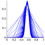
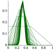
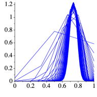
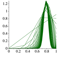
A156920	A055151	A290315	A290316

Figure 11: Normalized histograms (by their standard deviations or by $\sqrt{n}$) of A156920, A055151, A290315, and A290316 in the unit interval (namely, $[v^{\theta n}]P_{n}(v)$ with $\theta\in[0,1]$).

9.5.2 From $\mathscr{N}\bigl{(}{\frac{1}{4}n,\frac{1}{16}n}\bigr{)}$ to $\mathscr{N}\bigl{(}{\frac{1}{3}n,\frac{1}{18}n}\bigr{)}$

Consider A055151, which enumerates Motzkin paths of length $n$ with $k$ up steps. This sequence of polynomials satisfies the recurrence

$$(n+2)P_{n}(v)=((1+4v)n+2-4v)P_{n-1}(v)+2v(1-4v)P_{n-1}^{\prime}(v)\qquad(n\geqslant 1),$$

with $P_{0}(v)=1$. Changing $v\mapsto\frac{1}{4}v$ and then considering the reciprocal, we are led to the polynomials of type $\mathscr{M}(0,2,\frac{3}{2})$ (see § 5.6), which has the CLT $\mathscr{N}\bigl{(}{\frac{1}{4}n,\frac{1}{16}n;n^{-\frac{1}{2}}}\bigr{)}$. Reversing these two steps back and then integrating twice (due to the factor $(n+2)!$), we deduce that the OGF of $P_{n}$ is of the form

$$\sum_{n\geqslant 0}P_{n}(v)z^{n}=\frac{1-z-\sqrt{(1-z)^{2}-4vz^{2}}}{2vz^{2}},$$

yielding the CLT $\mathscr{N}\bigl{(}{\frac{1}{3}n,\frac{n}{18};n^{-\frac{1}{2}}}\bigr{)}$ by Theorem 2 with $\rho(v)=\bigl{(}{1+2\sqrt{v}}\bigr{)}^{-1}$; see Figure 11. An essentially the same sequence is A080159, and the reciprocal of $P_{n}$ corresponds to A107131.

Up steps in Motzkin paths	A055151 ($=$A080159)	$\mathscr{N}\bigl{(}{\frac{1}{3}n,\frac{1}{18}n;n^{-\frac{1}{2}}}\bigr{)}$
Reciprocal of A055151	A107131	$\mathscr{N}\bigl{(}{\frac{2}{3}n,\frac{1}{18}n;n^{-\frac{1}{2}}}\bigr{)}$

Recurrences of a similar form can be found in [169, 172, 173].

9.5.3 From $\mathscr{N}\bigl{(}{\frac{2}{3}n,\frac{1}{9}n}\bigr{)}$ to
$\mathscr{N}\left(\left(\frac{2q}{q-1}-\frac{q-1}{q-1-\log q}\right)n,\left(\frac{(q-1)^{2}-q(q-1-\log q)}{(q-1-\log q)^{2}}-\frac{2q}{(q-1)^{2}}\right)n\right)$

The polynomials defined by (see Section 5.1 for the class $\mathscr{T}$)

$$P_{n}(v):=n![z^{n}]\mathscr{T}\bigl{(}{q^{-1},2,1;v\mapsto qv,z\mapsto qz}\bigr{)}\qquad(q\geqslant 1),$$

satisfy the recurrence

$$P_{n}(v)=(2q^{2}vn+1-q(q+1)v)P_{n-1}(v)+qv(1-qv)P_{n-1}^{\prime}(v)\qquad(n\geqslant 1),$$

with $P_{0}(v)=1$. The coefficients are nonnegative when $q\geqslant 1$. When $q=1$, the $P_{n}$’s generate the second order Eulerian numbers A008517, and when $q=2,3$, they correspond to A290315 and A290316, respectively, which appeared in [156]. Since the EGF of $P_{n}$ equals (by (53))

$$\left(\frac{T_{2}\bigl{(}{qve^{-qv+q(1-qv)^{2}z}}\bigr{)}}{qv}\right)^{\frac{1}{q}}\frac{1-qv}{1-T_{2}\bigl{(}{qve^{-qv+q(1-qv)^{2}z}}\bigr{)}},$$

we deduce, by Theorem 2 with $\rho(v)=\frac{qv-1-\log qv}{q(qv-1)^{2}}$, the CLT (see Figure 11)

$$\mathscr{N}\left(\left(\frac{2q}{q-1}-\frac{q-1}{q-1-\log q}\right)n,\left(\frac{(q-1)^{2}-q(q-1-\log q)}{(q-1-\log q)^{2}}-\frac{2q}{(q-1)^{2}}\right)n;n^{-\frac{1}{2}}\right),$$

in contrast to the CLT $\mathscr{N}\bigl{(}{\frac{2}{3}n,\frac{1}{9}n;n^{-\frac{1}{2}}}\bigr{)}$ for $\mathscr{T}\bigl{(}{\frac{1}{q},2,1}\bigr{)}$. Note that $q>1$ need not to be an integer.

A290315	$\mathscr{N}\bigl{(}{\frac{3-4\log 2}{1-\log 2}n,\frac{-5+10\log 2-4\log^{2}2}{(1-\log 2)^{2}}n;n^{-\frac{1}{2}}}\bigr{)}$
A290316	$\mathscr{N}\bigl{(}{\frac{4-3\log 3}{2-\log 3}n,\frac{-16+18\log 3-3\log^{2}3}{2(2-\log 3)^{2}}n;n^{-\frac{1}{2}}}\bigr{)}$

9.5.4 Non-normal limit laws

Concrete examples with the factor “$1-v$” replaced by “$1-sv$” in the derivative term of (9) and leading to non-normal limit laws also exist and most of them are much simpler in nature. For example, the following sequences all lead to geometric limit laws.

OEIS	$e_{n}$	Type	$[v^{k}]P_{n}(v)$
A059268	$n$	$\mathscr{E}\langle\!\langle n+2v,-v(1-2v)\rangle\!\rangle$	$2^{k}$
A152920	$n-1$	$\mathscr{E}\langle\!\langle n+2v,-v(1-2v)\rangle\!\rangle$	$(2n-k)2^{k-1}$
A118413	$\frac{n(2n-1)}{2n+1}$	$\mathscr{E}\langle\!\langle n+2v,-v(1-2v)\rangle\!\rangle$	$(2n-1)2^{k-1}$
A233757	$\frac{n(2^{n}-1)}{2^{n+1}-1}$	$\mathscr{E}\langle\!\langle n+2v,-v(1-2v)\rangle\!\rangle$	$(2^{n}-1)2^{k-1}$
A130128	$n$	$\mathscr{E}\langle\!\langle n+1+2v,-v(1-2v)\rangle\!\rangle$	$(n-k+1)2^{k-1}$
A100851	$\frac{1}{2}n$	$\mathscr{E}\langle\!\langle n+3v,-v(1-3v)\rangle\!\rangle$	$2^{n}3^{k}$

9.6 Pólya urn models

Pólya’s urn schemes [179] are simple yet very useful in many modeling applications and are based on the ball-replacement matrix

ball color	white	black
white	$a$	$b$
black	$c$	$d$

and the initial configuration with $s_{0}\geqslant 1$ balls in the urn. At each stage draw a ball uniformly at random from the urn, and then return the ball together with $a$ white and $b$ black balls if its color is white, or $c$ white and $d$ black balls if its color is black. Repeat this procedure $n$ times and we are interested in the number $X_{n}$ of white balls after stage $n$. Assume $a+b=c+d=q\geqslant 1$ and $a\neq c$. Then the probability generating function $W_{n}(v)$ of $X_{n}$ satisfies the recurrence

$$W_{n}(v)=v^{c}W_{n-1}(v)+\frac{v^{a+1}-v^{c+1}}{s_{0}+q(n-1)}\,W_{n-1}^{\prime}(v)\qquad(n\geqslant 1),$$

with $W_{0}(v)=v^{X_{0}}$, where $0\leqslant X_{0}\leqslant s_{0}$ is a constant. This fits into our framework (9) if we consider $P_{n}(v)=W_{n}(v)\prod_{0\leqslant j<n}(s_{0}+qj)$, leading to the recurrence

$$P_{n}(v)=v^{c}(s_{0}+q(n-1))P_{n-1}(v)+\bigl{(}{v^{a+1}-v^{c+1}}\bigr{)}P_{n-1}^{\prime}(v)\qquad(n\geqslant 1),$$ (118)

with $P_{0}(v)=v^{s_{0}}$, which, in terms of the notations of (9), gives $\alpha(v)=qv^{c}$, $\beta(v)=\frac{v^{a+1}-v^{c+1}}{1-v}$ and $\gamma(v)=(s_{0}-q)v^{c}$. To apply our Theorem 1 on normal limit laws, we require $\alpha(v),\beta(v)$ and $\gamma(v)$ to be analytic in $|v|\leqslant 1$, which forces $a,c\geqslant-1$. Then the condition (11) becomes

$$\alpha(1)+2\beta(1)=a+b+2(c-a)>0\quad\Longrightarrow\quad\frac{a-c}{a+b}<\frac{1}{2},$$

and

$$\sigma^{2}=\frac{(a+b)bc(c-a)^{2}}{(b+c)^{2}(2c+b-a)}>0,$$

which requires that $b,c\geqslant 1$ (if both $b,c<0$, then $a>0$, which would imply $2c+b-a<0$). Thus if

$$a\geqslant 0,a\neq c,a+b=c+d\geqslant 1\;\text{and}\;b,c,2c+b-a\geqslant 1,$$

then the number of white balls follows the CLT

$$\mathscr{N}\left(\frac{c(a+b)}{b+c}\,n,\frac{(a+b)bc(c-a)^{2}}{(b+c)^{2}(2c+b-a)}\,n\right).$$

This result was derived in [8] by the method of moments but with a manipulation different from ours; see also [105] for the case when $a=d$ and $b=c$. The condition $a\geqslant 0$ can be relaxed but then additional conditions are needed to guarantee that $[v^{k}]P_{n}(v)\geqslant 0$; see [8] for details.

On the other hand, it is also possible to solve the PDE associated with the EGF of (118), and we obtain, in particular,

$$\rho(v)=\bigl{(}{1-v^{c-a}}\bigr{)}^{-\frac{a+b}{c-a}}\int_{v}^{1}t^{-a-1}\bigl{(}{1-t^{c-a}}\bigr{)}^{\frac{a+b}{c-a}-1}\,\mathrm{d}{t}.$$

We then deduce not only the same CLT but also a convergence rate. See also [96] for an analytic approach, [142, 151] for probabilistic approaches and [179] for a general introduction and more information.

If $a=0$, $c=1$, then, with $r=X_{0}$, $P_{n}(v)$ is essentially (up to a factor $v^{r}$) of type $\mathscr{T}(r,q,r)$ (see Section 5.1); in particular, we obtain the Eulerian numbers when $q=r=1$. Many other cases (normal or non-normal) can be further examined; we omit the details here.

9.7 $P_{n}^{\prime}(v)=(\alpha(v)n+\gamma(v))P_{n-1}(v)+\beta(v)(1-v)P_{n-1}^{\prime}(v)$

When the left-hand side of the Eulerian recurrence (9) is replaced by $P_{n}^{\prime}(v)$ (together with some boundary conditions), the same method of moments still applies, as already described in [129]. Note that in such cases, the presence of the crucial factor “$1-v$” in Eulerian recurrences is not essential for the application of the method of moments. We briefly consider two examples from [155] in the context of tree-like tableaux; see also [130]. The first one is of the form

$$P_{n}^{\prime}(v)=nP_{n-1}(v)+2(1-v)P_{n-1}^{\prime}(v)\qquad(n\geqslant 1),$$ (119)

with $P_{0}(v)=1$ and $P_{n}(1)=n!$, where $[v^{k}]P_{n}(v)$ equals the number of tree-like tableaux of size $n$ with $k$ occupied corners. By a direct calculation of the factorial moments, we see that

$$P_{n}(v)=\sum_{0\leqslant m\leqslant\lceil\frac{1}{2}n\rceil}\binom{n-m+1}{m}(n-m)!(v-1)^{m}\qquad(n\geqslant 0).$$

Thus the limit law of the coefficients is Poisson$(1)$ because

$$\frac{P_{n}(v)}{P_{n}(1)}\to e^{v-1}.$$

Another sequence of polynomials studied in [129, 155] is

$$Q_{n}^{\prime}(v)=2vnQ_{n-1}(v)+2(1-v^{2})Q_{n-1}^{\prime}(v)\qquad(n\geqslant 1),$$

with $Q_{0}(v)=1$ and $Q_{n}(1)=2^{n}n!$. Since the $Q_{n}$’s all contain even powers of $v$, we consider $R_{n}(v)=Q_{n}(\sqrt{v})$, which then satisfies the recurrence

$$R_{n}^{\prime}(v)=nR_{n-1}(v)+2(1-v)R_{n-1}^{\prime}(v)\qquad(n\geqslant 1),$$

with $R_{0}(v)=1$ and $R_{n}(1)=2^{n}n!$. This is of the same form as (119) but with a different boundary condition. By the same method of moments, we can show that the distribution of the coefficients of $R_{n}$ is asymptotically Poisson$(\frac{1}{2})$.

Interestingly, if we use the boundary condition $P_{n}(0)=0$ for $n\geqslant 1$ instead of $P_{n}(1)=n!$, then by solving the PDE satisfied by the OGF of $P_{n}$

$$z^{2}F_{z}^{\prime}+zF=(1-2(1-v)z)F_{v}^{\prime},$$

we obtain

$$F(z,v)=\frac{2(1-(1-v)z)}{1+\sqrt{1-4z+4(1-v)z^{2}}}.$$

This leads instead to the CLT $\bigl{(}{\frac{1}{4}n,\frac{1}{16}n;n^{-\frac{1}{2}}}\bigr{)}$ by Theorem 2 with $\rho(v)=\frac{1}{2}\bigl{(}{1+\sqrt{v}}\bigr{)}^{-1}$. Also in this case, $P_{n}(1)=\frac{1}{n+1}\binom{2n}{n}$. This coincides, up to a shift of indices, A091894 (Touchard distribution), which counts particularly the $231$-avoiding permutations according to the number of peaks. Furthermore,

$$[v^{k}z^{n}]F(z,v)=\frac{2^{n+1-2k}}{k}\binom{n-1}{2k-2}\binom{2k-2}{k-1}\qquad(1\leqslant k\leqslant\lceil\tfrac{n}{2}\rceil).$$

9.8 Extended Eulerian recurrences of Cauchy-Euler type

Similar to the Cauchy-Euler differential equations (see [50]), the same method of moments can be extended further to the equi-dimensional Eulerian recurrence,

$$e_{n}P_{n}(v)=\sum_{0\leqslant j\leqslant\ell}(1-v)^{j}P_{n-1}^{(j)}(v)\sum_{0\leqslant i\leqslant r-j}d_{j,i}(v)n^{i}\qquad(r\geqslant\ell\geqslant 1).$$ (120)

Consider first A091156, counting big ascents in Dyck paths of a given semilength:

$$P_{n}(v)=\frac{1}{n+1}\sum_{0\leqslant k\leqslant\lfloor\frac{1}{2}n\rfloor}\binom{n+1}{k}v^{k}\sum_{0\leqslant j\leqslant n-2k}\binom{k+j-1}{k-1}\binom{n+1-k}{n-2k-j}\qquad(n\geqslant 1).$$

Such $P_{n}$ satisfies the recurrence

$$P_{n}(v)=\frac{(1+3v)n+1-3v}{n+1}\,P_{n-1}(v)+\frac{2(4n-3)v(1-v)}{n(n+1)}P_{n-1}^{\prime}(v)+\frac{4v(1-v)^{2}}{n(n+1)}\,P_{n-1}^{\prime\prime}(v),$$

for $n\geqslant 1$ with $P_{0}(v)=1$, which can be proved by the OGF

$$\sum_{n\geqslant 0}P_{n}(v)z^{n}=\frac{1-\sqrt{1-4z+4(1-v)z^{2}}}{2z(1-(1-v)z)}.$$

We then deduce the CLT $\mathscr{N}\bigl{(}{\frac{1}{4}n,\frac{1}{16}n;n^{-\frac{1}{2}}}\bigr{)}$ by Theorem 2 with $\rho(v)=\frac{1}{2}\bigl{(}{1+\sqrt{v}}\bigr{)}^{-1}$.

We consider another example (with $\ell=r=2$ in (120)) from Legendre-Stirling permutations [83], where an extension of Eulerian numbers using Legendre-Stirling numbers [93] was studied:

$$D_{n}(v):=\sum_{j\geqslant 0}d_{n}(j)v^{j}=\frac{P_{n}(v)}{(1-v)^{3n+1}}=\frac{v}{1-v}\bigl{(}{vD_{n-1}(v)}\bigr{)}^{\prime\prime}.$$

Here $d_{n}(j)=d_{n}(j-1)+j(j+1)d_{n-1}(j)$ with $d_{0}(j)=1$ for $j\geqslant 0$ and $d_{n}(0)=0$ for $n\geqslant 1$, and

$$P_{n}(v) =v(3n-2)(3vn+2-3v)P_{n-1}(v)+2v(1-v)(3vn+1-3v)P_{n-1}^{\prime}(v)$$

$$\quad+v^{2}(1-v)^{2}P_{n-1}^{\prime\prime}(v)\qquad(n\geqslant 2),$$

with $P_{0}(v)=1$ and $P_{1}(v)=2v$. A CLT $\mathscr{N}\bigl{(}{\frac{6}{5}n,\frac{36}{175}n}\bigr{)}$ for the coefficients of $P_{n}$ was derived in [83] by the real-rootedness approach. The same CLT can aso be obtained by the method of moments; in particular, the mean and the variance are given by

$$\mathbb{E}(X_{n})=\frac{6n-1}{5}\quad\text{and}\quad\mathbb{V}(X_{n})=\frac{9(n-1)(12n+11)}{175(3n-1)}\qquad(n\geqslant 1).$$

However, we have no Berry-Esseen bound because no solution is available for the PDE

$$\left(v^{-2}\partial_{z}^{3}-z^{2}\partial_{z}^{2}-2z(1-v)\partial_{zv}^{2}-(1-v)^{2}\partial_{v}^{2}-4z\partial_{z}-2(1-v)\partial_{v}-2\right)F=0,$$

satisfied by the EGF $F(z,v):=v\sum_{n\geqslant 0}\frac{P_{n}(v)}{(3n)!}\,z^{3n}$. Note that the real-rootedness approach used in [83] can be refined to get the optimal Berry-Esseen bound.

9.9 A multivariate Eulerian recurrence

Enumerating simultaneously the number of descents $X_{n}$ in a random permutation of $n$ elements and that $Y_{n}$ of its inverse leads to the recurrence for the probability generating function of $X_{n}$ and $Y_{n}$ (see [36, 199, 234])

$$P_{n}(v,w) :=\mathbb{E}\bigl{(}{v^{X_{n}}w^{Y_{n}}}\bigr{)}$$

$$=\biggl{(}\frac{(n-1)(1-v)(1-w)}{n^{2}}+vw\left(1+\frac{1-v}{n}\,{\partial_{v}}\right)\left(1+\frac{1-w}{n}\,{\partial_{w}}\right)\biggr{)}P_{n-1}(v,w),$$

for $n\geqslant 1$, with $P_{0}(v,w)=1$. Recently, Chatterjee and Diaconis [46] proved the CLT $\mathscr{N}\bigl{(}{n,\frac{1}{6}n}\bigr{)}$ for $X_{n}+Y_{n}$, the total number of descents of a permutation and its inverse:

$$P_{n}(v,v)=\mathbb{E}\bigl{(}{v^{X_{n}+Y_{n}}}\bigr{)}=\frac{(1-v)^{2n+2}}{n!}\sum_{j,l\geqslant 0}\binom{jl+n-1}{n}v^{j+l}.$$

This paper also mentions six different ways to prove the CLT for Eulerian numbers: sum of $2$-dependent random variables, sum of Uniform$[0,1]$ random variables, Harper’s real-rootedness (sum of Bernoullis), Stein’s method, Bender’s analytic method and the method of moments, but none of the six applies to the coefficients of $[v^{k}]P_{n}(v,v)$; see also [198].

While a direct use of the method of moments fails, we show that it is possible to extend the method to establish the CLT for $X_{n}+Y_{n}$; in particular, we derive the asymptotics of the central moments $\mathbb{E}(\bar{X}_{n}+\bar{Y}_{n})^{m}$ through those of the joint moments $\mathbb{E}(\bar{X}_{n}^{j}\bar{Y}_{n}^{m-j})$, where $\bar{X}_{n}:=X_{n}-\frac{n+1}{2}$ and $\bar{Y}_{n}:=Y_{n}-\frac{n+1}{2}$, so that $\mathbb{E}(\bar{X}_{n})=\mathbb{E}(\bar{Y}_{n})=0$. For that purpose, we define

$$Q_{n}(s,t):=\exp\left(-\frac{n+1}{2}\,s-\frac{n+1}{2}\,t\right)P_{n}(e^{s},e^{t}),$$

which satisfies the recurrence

$$\begin{split}Q_{n}(s,t)&=\biggl{(}\frac{4(n-1)}{n^{2}}\,\sinh\bigl{(}{\tfrac{1}{2}s}\bigr{)}\sinh\bigl{(}{\tfrac{1}{2}t}\bigr{)}\biggr{)}Q_{n-1}(s,t)\\ &\quad+\left(\cosh\bigl{(}{\tfrac{1}{2}s}\bigr{)}-\frac{2}{n}\sinh\bigl{(}{\tfrac{1}{2}s}\bigr{)}\,{\partial_{s}}\right)\left(\cosh\bigl{(}{\tfrac{1}{2}t}\bigr{)}-\frac{2}{n}\sinh\bigl{(}{\tfrac{1}{2}t}\bigr{)}\,{\partial_{t}}\right)Q_{n-1}(s,t),\end{split}$$ (121)

for $n\geqslant 1$, with $Q_{0}(s,t)=e^{-\frac{1}{2}s-\frac{1}{2}t}$ and $Q_{1}(s,t)=1$. Write now

$$Q_{n}(s,t)=1+\sum_{m+l\geqslant 2}Q_{n;m,l}\,\frac{s^{m}t^{l}}{m!l!}\,\qquad(n\geqslant 1),$$

with $Q_{0;m,l}=(-1)^{m+l}2^{-m-l}$. Then by the recurrence (121) and induction, we see that

$$Q_{n;l,2m+1-l}=0\qquad(n\geqslant 1;0\leqslant l\leqslant 2m+1).$$

To compute the asymptotics of $Q_{n;l,2m-l}$, we use the recurrence

$$Q_{n;m,l}=\left(1-\frac{m}{n}\right)\left(1-\frac{l}{n}\right)Q_{n-1;m,l}+R_{n;m,l},$$

where

$$\begin{split}R_{n;m,l}&=\frac{n-1}{n^{2}}\sum_{\begin{subarray}{c}0\leqslant i\leqslant\lfloor\frac{1}{2}(m-1)\rfloor\\ 0\leqslant j\leqslant\lfloor\frac{1}{2}(l-1)\rfloor\end{subarray}}\binom{m}{2i+1}\binom{l}{2j+1}2^{-2i-2j}Q_{n-1;m-2i-1,l-2j-1}\\ &\quad+\sum_{\begin{subarray}{c}0\leqslant i\leqslant\lfloor\frac{1}{2}m\rfloor\\ 0\leqslant j\leqslant\lfloor\frac{1}{2}l\rfloor\\ i+j\geqslant 1\end{subarray}}\binom{m}{2i}\binom{l}{2j}2^{-2i-2j}Q_{n-1;m-2i,l-2j}\left(1-\frac{m-2i}{n(2i+1)}\right)\left(1-\frac{l-2j}{n(2j+1)}\right).\end{split}$$ (122)

Then by induction, we show that

$$Q_{n;2m-l,l}\sim d(l)d(2m-l)\sigma_{n}^{2m}\qquad(0\leqslant l\leqslant 2m;m\geqslant 0),$$ (123)

where $\sigma_{n}^{2}:=\frac{1}{12}n$, $d(2j+1)=0$ and $d(2j)=(2j-1)!!=\frac{(2j)!}{j!2^{j}}$. See Appendix A for details. By the expansion

$$\mu_{m}:=\mathbb{E}\bigl{(}{\bar{X}_{n}+\bar{Y}_{n}}\bigr{)}^{m}=\sum_{0\leqslant l\leqslant m}\binom{m}{l}Q_{n;m-l,l},$$

we see that $\mu_{2m+1}=0$ because $Q_{n;2m+1-l,l}=0$; furthermore, using the estimate (123), we deduce that

$$\mu_{2m}\sim\sigma_{n}^{2m}\sum_{0\leqslant l\leqslant m}\binom{2m}{2l}d(2l)d(2m-2l)=d(2m)2^{m}\sigma_{n}^{2m}.$$

We then conclude that $X_{n}+Y_{n}\sim\mathscr{N}\bigl{(}{n,\frac{1}{6}n}\bigr{)}$.

A type $B$ analogue is given in [234] and the same CLT $\mathscr{N}\bigl{(}{n,\frac{1}{6}n}\bigr{)}$ can be established by the same approach.

10 The degenerate case: $\beta(v)\equiv 0\Longrightarrow P_{n}(v)=a_{n}(v)P_{n-1}(v)$

For completeness, we briefly discuss a special class of Eulerian recurrences of the form (without derivative terms)

$$P_{n}(v)=a_{n}(v)P_{n-1}(v)\qquad(n\geqslant 1),$$ (124)

with $P_{0}(v)$ given. Typical examples include binomial coefficients with $a_{n}(v)=1+v$ and Stirling numbers of the first kind with $a_{n}(v)=n-1+v$. Assume that $[v^{k}]a_{n}(v)\geqslant 0$, $a_{n}(v)$ is analytic in $|v|\leqslant 1$ and $a_{n}(1)>0$ for $k,n\geqslant 0$. Define $X_{n}$ as in (10). Then, with $a_{0}(v):=P_{0}(v)$, $X_{n}$ is expressible as the sum of independent random variables:

$$X_{n}=\sum_{0\leqslant j\leqslant n}Y_{j},\quad\text{where}\quad\mathbb{E}\bigl{(}{v^{Y_{j}}}\bigr{)}=\frac{a_{j}(v)}{a_{j}(1)}.$$

Thus $X_{n}$ is asymptotically normally distributed if the Lyapunov condition (see [95]) holds:

$$\sum_{0\leqslant j\leqslant n}\mathbb{E}|Y_{j}-\mathbb{E}(Y_{j})|^{3}=o(\mathbb{V}(X_{n})^{3/2}).$$

This condition is not optimal but is simpler to use in a setting like ours. In particular, it holds when each $Y_{j}$ is bounded.

A simple linear framework

To be more precise, we consider the linear framework when $a_{n}(v)=\alpha(v)n+\gamma(v)$, where $\alpha$ and $\gamma$ are in most cases polynomials. Then we have

$$\mathbb{E}(X_{n})=\frac{P_{0}^{\prime}(1)}{P_{0}(1)}+\sum_{1\leqslant j\leqslant n}\frac{\alpha^{\prime}(1)j+\gamma^{\prime}(1)}{\alpha(1)j+\gamma(1)}.$$

It follows that

$$\mathbb{E}(X_{n})=\begin{cases}\mu(\alpha)n+\nu\log n+O(1),&\text{if }\mu(\alpha)>0;\\ \frac{\gamma^{\prime}(1)}{\alpha(1)}\log n+O(1),&\text{if }\mu(\alpha)=0,\alpha(1),\gamma^{\prime}(1)>0;\\ \mu(\gamma)n+O(1),&\text{if }\mu(\alpha)=\alpha(1)=0,\mu(\gamma)>0,\\ \end{cases}$$

where

$$\mu(f):=\frac{f^{\prime}(1)}{f(1)},\quad\text{and}\quad\nu:=\frac{\alpha(1)\gamma^{\prime}(1)-\alpha^{\prime}(1)\gamma(1)}{\alpha(1)^{2}}.$$

For the variance, with the notation

$$\sigma^{2}(f):=\frac{f^{\prime}(1)}{f(1)}+\frac{f^{\prime\prime}(1)}{f(1)}-\left(\frac{f^{\prime}(1)}{f(1)}\right)^{2},$$

we have

$$\mathbb{V}(X_{n})=\begin{cases}\sigma^{2}(\alpha)n+O(\log n),&\text{if }\sigma^{2}(\alpha)>0;\\ \varsigma\log n+O(1),&\text{if }\sigma^{2}(\alpha)=0,\alpha(1),\varsigma>0;\\ \sigma^{2}(\gamma)n+O(1),&\text{if }\sigma^{2}(\alpha)=\alpha(1)=0,\sigma^{2}(\gamma)>0,\\ \end{cases}$$

where

$$\varsigma:=\frac{\gamma^{\prime}(1)+\gamma^{\prime\prime}(1)}{\alpha(1)}-\frac{2\alpha^{\prime}(1)\gamma^{\prime}(1)}{\alpha(1)^{2}}+\frac{\gamma(1)\alpha^{\prime}(1)^{2}}{\alpha(1)^{3}}.$$

In all cases, the distribution of $X_{n}$ is asymptotically normal if $\mathbb{V}(X_{n})\to\infty$:

$$X_{n}\sim\begin{cases}\mathscr{N}\bigl{(}{\mu(\alpha)n,\sigma^{2}(\alpha)n}\bigr{)},&\text{if }\sigma^{2}(\alpha)>0;\\ \mathscr{N}\bigl{(}{\mu(\alpha)n+\nu\log n,\varsigma\log n}\bigr{)},&\text{if }\sigma^{2}(\alpha)=0,\varsigma>0;\\ \mathscr{N}\bigl{(}{\mu(\gamma)n,\sigma^{2}(\gamma)n}\bigr{)},&\text{if }\sigma^{2}(\alpha)=\alpha(1)=0,\sigma^{2}(\gamma)>0.\end{cases}$$

Applications

The literature and the database OEIS abound with examples satisfying (124), and they are mostly of a simpler nature when compared with (9). The prototypical example is binomial coefficients $\binom{n}{k}$: A007318 (or A135278) for which $a_{n}(v)=1+v$. We then obtain the CLT $\mathscr{N}\bigl{(}{\frac{1}{2}n,\frac{1}{4}n}\bigr{)}$, a result first established by de Moivre in 1738 [73]. Another 80 OEIS sequences of the form (124) with $a_{n}(v)=e_{n}(1+v)$ are collected in Appendix B, where $e_{n}$ is either a constant or a sequence of $n$. We get the same CLT $\mathscr{N}\bigl{(}{\frac{1}{2}n,\frac{1}{4}n}\bigr{)}$ for the coefficients.

We also identified another 182 sequences satisfying (124) with $a_{n}(v)=p+qv+rv^{2}$ with $p,q,r$ nonnegative integers. The corresponding coefficients follow the CLT

$$\mathscr{N}\left(\frac{q+2r}{p+q+r}\,n,\frac{pq+4pr+qr}{(p+q+r)^{2}}\,n\right);$$

see Appendix B for the tables of these sequences.

Examples for which $\alpha(v),\sigma^{2}(\alpha)\neq 0$ are scarce:

A059364$(n,k)$ $=\sum_{k\leqslant j<n}\binom{j}{k}\genfrac{[}{]}{0.0pt}{}{n}{n-j}$	$a_{n}(v)=(1+v)n+1$	$\mathscr{N}\bigl{(}{\frac{1}{2}n,\frac{1}{4}n}\bigr{)}$
A088996: reciprocal of A059364	$(1+v)n-1$	$\mathscr{N}\bigl{(}{\frac{1}{2}n,\frac{1}{4}n}\bigr{)}$
A322225	$(1+v^{2})n+v$	$\mathscr{N}\bigl{(}{n,n}\bigr{)}$
A322235	$(1+2v^{2})n+v$	$\mathscr{N}\bigl{(}{\frac{4}{3}n,\frac{8}{9}n}\bigr{)}$

Here $\genfrac{[}{]}{0.0pt}{}{n}{k}$ denotes the unsigned Stirling numbers of the first kind (A132393, A094638, A130534), another prototypical example with log-variance CLT.

We now group other examples with logarithmic variance according as $\mu(\alpha)>0$ or $\mu(\alpha)=0$, respectively.

Polynomials with $\mu(\alpha)>0$ and $\sigma^{2}(\alpha)=0$, and $\varsigma>0$

OEIS	$a_{n}(v)$	Initial	CLT
A094638	$vn+1$	$P_{0}(v)=1$	$\mathscr{N}(n-\log n,\log n)$
A109692	$2vn+1-v$	$P_{0}(v)=1$	$\mathscr{N}(n-\frac{1}{2}\log n,\frac{1}{2}\log n)$
A145324	$vn+1+v$	$P_{0}(v)=1$	$\mathscr{N}(n-\log n,\log n)$
A196841	$vn+1+v$	$P_{1}(v)=1+v$	$\mathscr{N}(n-\log n,\log n)$
A196842	$vn+1+v$	$P_{2}(v)=1+3v+2v^{2}$	$\mathscr{N}(n-\log n,\log n)$
A196843	$vn+1+v$	$P_{3}(v)=1+6v+11v^{2}+6v^{3}$	$\mathscr{N}(n-\log n,\log n)$
A196844	$vn+1+v$	$P_{4}(v)=1+10v+35v^{2}+50v^{3}+24v^{4}$	$\mathscr{N}(n-\log n,\log n)$
A196845	$vn+1+2v$	$P_{0}(v)=1$	$\mathscr{N}(n-\log n,\log n)$
A196846	$vn+1+2v$	$P_{2}(v)=1+3v+2v^{2}$	$\mathscr{N}(n-\log n,\log n)$
A201949	$vn+1-v+v^{2}$	$P_{0}(v)=1$	$\mathscr{N}(n,\log n)$
A249790	$vn+1+v^{2}$	$P_{0}(v)=1$	$\mathscr{N}(n,\log n)$
A291845	$2vn+1-v+v^{2}$	$P_{0}(v)=1$	$\mathscr{N}(n,\log n)$
A324960	$vn+1+2v+v^{2}$	$P_{0}(v)=1$	$\mathscr{N}(n,2\log n)$

Polynomials with $\mu(\alpha)=\sigma^{2}(\alpha)=0$, and $\varsigma>0$

OEIS	$a_{n}(v)$	Initial	CLT
A028338	$2n-1+v$	$P_{0}(v)=1$	$\mathscr{N}(\frac{1}{2}\log n,\frac{1}{2}\log n)$
A125553	$n+2v$	$P_{0}(v)=2$	$\mathscr{N}(2\log n,2\log n)$
A130534	$n+v$	$P_{0}(v)=1$	$\mathscr{N}(\log n,\log n)$
A132393	$n-1+v$	$P_{0}(v)=1$	$\mathscr{N}(\log n,\log n)$
A136124	$n+1+v$	$P_{0}(v)=1$	$\mathscr{N}(\log n,\log n)$
A137320	$n-1+2v$	$P_{0}(v)=1$	$\mathscr{N}(2\log n,2\log n)$
A137339	$n-1+3v$	$P_{0}(v)=1$	$\mathscr{N}(3\log n,3\log n)$
A143491	$n+1+v$	$P_{0}(v)=1$	$\mathscr{N}(\log n,\log n)$
A143492	$n+2+v$	$P_{0}(v)=1$	$\mathscr{N}(\log n,\log n)$
A143493	$n+3+v$	$P_{0}(v)=1$	$\mathscr{N}(\log n,\log n)$
A161198	$2n-1+2v$	$P_{0}(v)=1$	$\mathscr{N}(\log n,\log n)$
A180013	$\frac{1+n}{n}\left(n-1+v\right)$	$P_{0}(v)=1$	$\mathscr{N}(\log n,\log n)$
A204420	$\left(2n-1\right)\left(2n-2+v\right)$	$P_{0}(v)=1$	$\mathscr{N}(\frac{1}{2}\log n,\frac{1}{2}\log n)$
A216118	$\frac{n+3}{n-1}\left(n+v\right)$	$P_{1}(v)=1+v$	$\mathscr{N}(\log n,\log n)$
A225470	$3n-1+v$	$P_{0}(v)=1$	$\mathscr{N}(\frac{1}{3}\log n,\frac{1}{3}\log n)$
A286718	$3n-2+v$	$P_{0}(v)=1$	$\mathscr{N}(\frac{1}{3}\log n,\frac{1}{3}\log n)$
A225471	$4n-1+v$	$P_{0}(v)=1$	$\mathscr{N}(\frac{1}{4}\log n,\frac{1}{4}\log n)$
A290319	$4n-3+v$	$P_{0}(v)=1$	$\mathscr{N}(\frac{1}{4}\log n,\frac{1}{4}\log n)$
A225477	$3n-1+3v$	$P_{0}(v)=1$	$\mathscr{N}(\log n,\log n)$
A225478	$4n-1+4v$	$P_{0}(v)=1$	$\mathscr{N}(\log n,\log n)$
A254881	$\left(n-1+v\right)\left(n+v\right)$	$P_{0}(v)=1$	$\mathscr{N}(2\log n,2\log n)$

Historically, the Stirling numbers of the first kind numbers were found as early as the 17th century in Thomas Harriot’s unpublished manuscripts in addition to James Stirling’s book Methodus Differentialis published in 1730; see [13, p. 61] and [152] for more historical notes. The CLT for $\genfrac{[}{]}{0.0pt}{}{n}{k}$ first appeared in Goncharov’s 1942 paper [116] (see also [94, 117]) in the form of cycles in permutations.

$a_{n}(v)$ depending on the parity of $n$

OEIS	$a_{n}(v)$ ($n$ odd)	$a_{n}(v)$ ($n$ even)	Initial	CLT
A060523	$n$	$n-1+v$	$P_{0}(v)=1$	$\mathscr{N}(\frac{1}{2}\log n,\frac{1}{2}\log n)$
A064861	$1+2v$	$1+v$	$P_{0}(v)=1$	$\mathscr{N}(\frac{7}{12}n,\frac{17}{72}n)$
A152815	$1$	$1+v$	$P_{0}(v)=1$	$\mathscr{N}(\frac{1}{4}n,\frac{1}{8}n)$
A152842	$1+3v$	$1+v$	$P_{0}(v)=1$	$\mathscr{N}(\frac{5}{8}n,\frac{7}{32}n)$
A188440	$1$	$1+2v$	$P_{0}(v)=1$	$\mathscr{N}(\frac{1}{3}n,\frac{1}{9}n)$
A246117	$\frac{1}{2}(n-1)+v$	$\frac{1}{2}n+v$	$P_{0}(v)=1$	$\mathscr{N}(2\log n,2\log n)$
A274496	$2$	$1+v$	$P_{0}(v)=1$	$\mathscr{N}(\frac{1}{4}n,\frac{1}{8}n)$
A274498	$3$	$1+2v$	$P_{0}(v)=1$	$\mathscr{N}(\frac{1}{3}n,\frac{1}{9}n)$
A026519	$1+v+v^{2}$	$1+v^{2}$	$P_{0}(v)=1$	$\mathscr{N}(n,\frac{5}{6}n)$
A026536	$1+v^{2}$	$1+v+v^{2}$	$P_{0}(v)=1$	$\mathscr{N}(n,\frac{5}{6}n)$
A026552	$1+v^{2}$	$1+v+v^{2}$	$P_{1}(v)=1+v+v^{2}$	$\mathscr{N}(n,\frac{5}{6}n)$

Nonlinear $a_{n}(v)$

Let $p_{n}$ denote the $n$th prime and $f_{n}$ the $n$th Fibonacci number. Then by the prime number theorem it is known that $p_{n}\sim n\log n$; also $f_{n}\sim 5^{-\frac{1}{2}}\phi^{-n-1}$, where $\phi=\frac{\sqrt{5}-1}{2}$ is the golden ratio. Then the following CLTs follow from these estimates and Lyapunov’s condition.

OEIS	$a_{n}(v)$	Initial	CLT
A096294	$p_{n}-1+v$	$P_{0}(v)=1$	$\mathscr{N}(\log\log n,\log\log n)$
A260613	$1+p_{n}v$	$P_{0}(v)=1$	$\mathscr{N}(n-\log\log n,\log\log n)$
A130405	$f_{n}+f_{n-1}v$	$P_{0}(v)=1$	$\mathscr{N}\bigl{(}{\frac{\phi}{1+\phi}n,\frac{\phi}{(1+\phi)^{2}}n}\bigr{)}$

A CLT $\mathscr{N}\bigl{(}{\frac{1}{2}n,\frac{1}{6}n}\bigr{)}$

Sequence A220884 is not of the type (124) but has a similar product form

$$P_{n}(v)=\prod_{1\leqslant j<n}(jv+n+1-j),$$

which leads to the CLT $\mathscr{N}\bigl{(}{\frac{1}{2}n,\frac{1}{6}n}\bigr{)}$.

Non-normal limit laws

Non-normal limit laws arise when the variance remains bounded and the analysis is simple because the probability generating function (PGF) tends to a finite limit. Consider the case when $a_{n}(v)=e_{n}+v$, where $\sum_{j\geqslant 1}e_{j}^{-1}$ is convergent. Then

$$\mathbb{E}\bigl{(}{v^{X_{n}}}\bigr{)}=\frac{P_{n}(v)}{P_{n}(1)}=\prod_{1\leqslant j\leqslant n}\frac{e_{j}+v}{e_{j}+1}\to\prod_{j\geqslant 1}\frac{1+\frac{v}{e_{j}}}{1+\frac{1}{e_{j}}}.$$

When $a_{n}(v)=e_{n}v+1$, we consider $n-X_{n}$, and we get the same limit law. Some examples of these types are collected in the following table ($P_{0}(v)=1$ in all cases).

OEIS	$a_{n}(v)$	$\begin{array}[]{c}\text{PGF of the}\\ \text{limit law}\end{array}$	OEIS	$a_{n}(v)$	$\begin{array}[]{c}\text{PGF of the}\\ \text{limit law}\end{array}$
A008955	$vn^{2}+1$	$\frac{\sinh\bigl{(}{\pi\sqrt{v}}\bigr{)}}{\sqrt{v}\sinh(\pi)}$	A008956	$v(2n-1)^{2}+1$	$\frac{\cosh\bigl{(}{\frac{1}{2}\pi\sqrt{v}}\bigr{)}}{\cosh\bigl{(}{\frac{1}{2}\pi}\bigr{)}}$
A108084	$2^{n}+v$	$\frac{\prod_{j\geqslant 1}\bigl{(}{1+2^{-j}v}\bigr{)}}{\prod_{j\geqslant 1}\bigl{(}{1+2^{-j}}\bigr{)}}$	A128813	$\frac{1}{2}vn(n+1)+1$	$\frac{\cos\bigl{(}{\frac{1}{2}\pi\sqrt{1-8v}}\bigr{)}}{v\cosh\bigl{(}{\frac{\sqrt{7}}{2}\pi}\bigr{)}}$
A160563	$(2n-1)^{2}+v$	$\frac{\cosh\bigl{(}{\frac{\pi}{2}\sqrt{v}}\bigr{)}}{\cosh\bigl{(}{\frac{\pi}{2}}\bigr{)}}$	A173007	$3^{n}+v$	$\frac{\prod_{j\geqslant 1}\bigl{(}{1+3^{-j}v}\bigr{)}}{\prod_{j\geqslant 1}\bigl{(}{1+3^{-j}}\bigr{)}}$
A173008	$4^{n}+v$	$\frac{\prod_{j\geqslant 1}\bigl{(}{1+4^{-j}v}\bigr{)}}{\prod_{j\geqslant 1}\bigl{(}{1+4^{-j}}\bigr{)}}$	A249677	$vn^{3}+1$	$\frac{\prod_{j\geqslant 1}\bigl{(}{1+j^{-3}v}\bigr{)}}{\prod_{j\geqslant 1}\bigl{(}{1+j^{-3}}\bigr{)}}$
A269944	$(n-1)^{2}+v$	$\frac{\sinh\bigl{(}{\pi\sqrt{v}}\bigr{)}}{\sqrt{v}\sinh(\pi)}$	A269947	$(n-1)^{3}+v$	$v\frac{\prod_{j\geqslant 1}\bigl{(}{1+j^{-3}v}\bigr{)}}{\prod_{j\geqslant 1}\bigl{(}{1+j^{-3}}\bigr{)}}$

11 Conclusions

In connecting Eulerian numbers to descents in permutations in the preface of Petersen’s book [200], Richard Stanley writes: “Who could believe that such a simple concept would have a deep and rich theory, with close connections to a vast number of other subjects?” We demonstrated in this paper, through a considerable number (more than 500) of examples from the literature and the OEIS database, that not only have the Eulerian numbers been very fruitfully explored, but its simple extension to Eulerian recurrences is very effective and powerful in modeling many different laws—a prolific source of various phenomena indeed, although we limited our study mostly to linear (in $n$) factors $a_{n}(v)$ and $b_{n}(v)$. The combined use of an elementary approach (method of moments) and an analytic one (notably Theorem 2) also proved to be functional, handy and very successful. To see further the modeling versatility of Eulerian recurrences, we conclude with a few special Eulerian examples from OEIS of the recursive form $\mathscr{E}\langle\!\langle a_{n}(v),b_{n}(v)\rangle\!\rangle$, where $a_{n}(v)$ and $b_{n}(v)$ are quadratic either in $n$ or in $v$.

A mixture of two Betas $\Longrightarrow$ Uniform

Writing all rational numbers $\frac{p}{q}\in(0,1)$ as ordered pairs $(p,q)$ gives sequence A181118 or the polynomials

$$P_{n}(v)=\sum_{1\leqslant k\leqslant n}\bigl{(}{kv^{2k}+(n+1-k)v^{2k-1}}\bigr{)},$$

which satisfy the recurrence

$$P_{n}\in\mathscr{E}_{1}\left\langle\!\left\langle\frac{2n^{2}+v^{2}n-v}{(n-1)(2n-1)},-\frac{nv(1+v)}{(n-1)(2n-1)};v+v^{2}\right\rangle\!\right\rangle.$$

The limit distribution is Uniform$[0,2]$ although the random variable is a mixture of two Betas; see Figure 12. On the other hand, the sequence A215655 is twice A181118.

A mixture of two normals

The Eulerian recurrence is also capable of describing the binomial distribution concatenated twice: $P_{n}(v):=(1+v)^{n}(1+v^{n+1})$, which corresponds to A152198 and satisfies

$$P_{n}\in\mathscr{E}\left\langle\!\left\langle\frac{(1+2v-v^{2})n-v(1-v)}{n},-\frac{v(1+v)}{n};1+v\right\rangle\!\right\rangle.$$

On the other hand, the sequence A188440 corresponds to the polynomials $\sum_{0\leqslant k\leqslant\lfloor\frac{n}{2}\rfloor}\binom{\lfloor\frac{1}{2}n\rfloor}{k}v^{k}$. If we concatenate the two polynomial rows with the same row number $\lfloor\frac{1}{2}n\rfloor$ and read them sequentially as one, we get

$$P_{n}\in\mathscr{E}\left\langle\!\left\langle\frac{(1+4v-2v^{2})n-2v(1-v)}{n},-\frac{v(1+2v)}{n};1+v\right\rangle\!\right\rangle,$$

and the resulting distributions are similar to those of A152198.

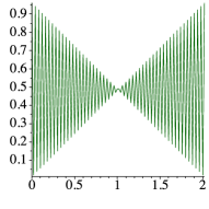
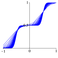
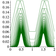
Figure 12: Histograms of A181118 when $n=50$ (left) and of A152198 for $n=3,\dots,50$ (right), and the (normalized) distribution functions of A152198 (middle).

Degenerate limit law

While the recurrence $P_{n}\in\mathscr{E}\langle\!\langle\frac{n+v^{2}}{n},-\frac{v(1+v)}{2n};1\rangle\!\rangle$ leads to a uniform limit law (see Section 8.2), changing the minus sign to a positive one

$$P_{n}\in\mathscr{E}\left\langle\!\left\langle\frac{n+v^{2}}{n},\frac{v(1+v)}{2n};1\right\rangle\!\right\rangle$$

gives the closed-form solution $P_{n}(v)=1+nv^{2}$.

Similarly, the recurrence $P_{n}\in\mathscr{E}\langle\!\langle\frac{n+v}{n},-\frac{v}{n};1\rangle\!\rangle$ leads to a uniform limit law (A000012, as we examined in § 8.1.1), but $P_{n}\in\mathscr{E}\langle\!\langle\frac{n+v}{n},\frac{v}{n};1\rangle\!\rangle$ gives $P_{n}(v)=1+nv$, and yields the degenerate limit law, which (when read sequentially) corresponds to A057979, and up to different initial conditions, to A133622, A152271 and A158416. Note that these four sequences are not triangular sequences.

Another normal limit law

For the examples examined in this section, if we have no a priori information about the solution, then the method of moments still works well except for the normal mixtures. But the analytic method will generally become more messy as the PDEs involved will have higher orders. To see this, we look briefly at another example A136267 (with normal limit law), which is defined via Narayana numbers (see Section 5.5.3) by

$$P_{n}(v)=\frac{1}{1+v}\sum_{1\leqslant k\leqslant 2n+2}\binom{2n+1}{k-1}\binom{2n+2}{k-1}\frac{v^{k-1}}{k},$$

a polynomial of degree $2n$. Such polynomials satisfy the rather cumbersome recurrence

$$P_{n}\in\mathscr{E}\left\langle\!\left\langle\frac{2(1+10v+5v^{2})n^{2}+(5+24v+3v^{2})n+3(1+2v-v^{2})}{(n+1)(2n+3)},\frac{(4n+3)v(1+v)}{(n+1)(2n+3)};1\right\rangle\!\right\rangle.$$

To prove this, we see first that the OGF of $P_{n}(v)$ satisfies the PDE

$$2z^{2}(1-(1+10v+5v^{2})z)\partial_{z}^{2}Y-4vz^{2}(1-v^{2})\partial_{z}\partial_{v}Y+z(7-(11+84v+33v^{2})z)\partial_{z}Y$$

$$-7vz(1-v^{2})\partial_{v}Y+(3-10(1+5v+v^{2})z)Y-3=0,$$

with $Y(0,v)=1$. Although this equation is not easy to solve, it is easy to check that the solution is given by

$$Y(z,v):=\frac{f\bigl{(}{\sqrt{z},v}\bigr{)}+f\bigl{(}{-\sqrt{z},v}\bigr{)}}{2v(1+v)z},$$

where $f$ is the OGF for Narayana numbers; see (77). By the recurrences in Section 2.5, the mean and the variance are

$$\mathbb{E}(X_{n})=n,\quad\text{and}\quad\mathbb{V}(X_{n})=\frac{n(n+1)}{4n+3}\qquad(n\geqslant 1),$$

and the asymptotic normality $\mathscr{N}\bigl{(}{n,\frac{1}{4}n}\bigr{)}$ can either be derived by the method of moments or by the CLT for Narayana numbers. The complex-analytic approach (Theorem 2) also applies here with $\rho(v)=(1+v)^{-4}$, and we get an optimal convergence rate in the CLT $\mathscr{N}\bigl{(}{n,\frac{1}{4}n;n^{-\frac{1}{2}}}\bigr{)}$. Yet another approach is to apply Stirling’s formula to $[v^{k}]P_{n}(v)$ and derive the corresponding LLT when $k=n+o\bigl{(}{n^{\frac{2}{3}}}\bigr{)}$, but this approach is often limited to the situations when simple closed-form expression is available.

Perspectives

A natural, fundamental question regarding more general Eulerian recurrence $P_{n}\in\mathscr{E}\langle\!\langle a_{n}(v),b_{n}(v)\rangle\!\rangle$ is “are there simple criteria (on $a_{n}(v)$ and $b_{n}(v)$) to guarantee the nonnegativity of the coefficients $[v^{k}]P_{n}(v)$?”

On the other hand, from a methodological point of view, how to address the finer properties such as local limit theorems and large deviations by a more systematic approach? Much remains to be clarified.

Bóna writes in [18]: “While Eulerian numbers have been given plenty of attention during the last 200 years, most of the research was devoted to analytic concepts.” Despite the large literature on analytic aspects, a more complete compilation of the Eulerian recurrences seems lacking and this paper also aims to provide an attempt to gather more examples and types of Eulerian recurrences, focusing on distributional aspect of the coefficients. We believe that such an extensive compilation will also be helpful for the study of other properties of Eulerian recurrences and related structures.

Our method of moments relies crucially on the presence of the factor “$1-v$” in the derivative term in (9); it fails when $1-v$ is not there as we already saw many examples in Section 9.5. Such recurrences also occur frequently in combinatorics and a systematic study of the corresponding distributional properties of the coefficients will be given elsewhere.

Finally, from a computational point of view, the Eulerian recurrence is a Markovian one in that the $n$th row of the polynomials $P_{n}$ depends only on $P_{n-1}$ and its derivative. This property not only facilites the systematic computer search through all OEIS sequences but also provides a good framework for mathematical analysis; yet the total number (594) we worked out is still relatively small compared with the 25,000+ nonnegative polynomial sequences in OEIS (over a total of 327,000+). Although many such polynomial sequences do not have combinatorial or structural interpretations or are rather artificially constructed, they do provide a very rich and valuable source for the study of various properties such as the distribution of the coefficients, and that of the zeros. A complete characterization of the corresponding limit laws is of special methodological and phenomenal interest but seems too early at this stage.

A Proof of (123)

By induction hypothesis, we see that the largest terms in the sum expression (122) of $R_{n;2m-l,l}$ occur when $(i,j)=(0,1)$ and $(i,j)=(1,0)$, giving

$$R_{n;2m-l,l}\sim\frac{1}{4}\binom{2m-l}{2}Q_{n-1;2m-l-2,l}+\frac{1}{4}\binom{l}{2}Q_{n-1;2m-l,l-2},$$

where $Q$ with negative indices are interpreted as zero. By (123)

$$R_{n;2m-l,l}\sim C_{2m-l,l}\sigma_{n}^{2m-2},$$ (125)

where

$$C_{2m-l,l}:=\frac{d(l)d(2m-l-2)}{4}\binom{2m-l}{2}+\frac{d(2m-l)d(l-2)}{4}\binom{l}{2}.$$

Consider now the recurrence

$$x_{n}=\left(1-\frac{m}{n}\right)\left(1-\frac{l}{n}\right)x_{n-1}+y_{n}\qquad(n\geqslant n_{0}),$$

with the given initial condition $x_{n_{0}}$, where $n_{0}:=\max\{m,l\}+1$. Then (with $y_{n_{0}}:=x_{n_{0}}$)

$$x_{n}=\frac{(n-m)!(n-l)!}{n!^{2}}\sum_{n_{0}\leqslant j\leqslant n}\frac{j!^{2}\,y_{j}}{(j-m)!(j-l)!}\qquad(n\geqslant m).$$

From this exact expression, we deduce the asymptotic transfer:

$$\text{if }y_{n}\sim cn^{\alpha},\text{ then }x_{n}\sim\frac{c}{m+l+\alpha+1}\,n^{\alpha+1}\qquad(m+l+\alpha>0).$$

Applying this transfer, we see that

$$Q_{n;2m-l,l}\sim\frac{4C_{2m-l,l}}{m}\,\sigma_{n}^{2m}.$$

Now the leading constant equals

$$\frac{d(l)d(2m-l-2)}{m}\binom{2m-l}{2}+\frac{d(2m-l)d(l-2)}{m}\binom{l}{2}=d(l)d(2m-l),$$

after a straightforward simplification. By induction, this proves (123).

B Some OEIS sequences satisfying $P_{n}(v)=a_{n}(v)P_{n-1}(v)$

In this Appendix, we collect some OEIS sequences satisfying the recurrence $P_{n}(v)=a_{n}(v)P_{n-1}(v)$ and give their limit laws. For convenience, we use the notation $\mathscr{E}_{m}\langle\!\langle a_{n}(v),0;B(v)\rangle\!\rangle$ for an abbreviation of $\mathscr{E}\langle\!\langle a_{n}(v),0;P_{m}(v)=B(v)\rangle\!\rangle$ (those without subscripts stand for $\mathscr{E}_{0}\langle\!\langle a_{n}(v),0;B(v)\rangle\!\rangle$ as above).

$a_{n}(v)=c\Longrightarrow\mathscr{N}\bigl{(}{\frac{1}{2}n,\frac{1}{4}n}\bigr{)}$, where $c$ is a constant

OEIS	Type	OEIS	Type
A007318	$\mathscr{E}\langle\!\langle 1+v,0;1\rangle\!\rangle$	A028262	$\mathscr{E}_{2}\langle\!\langle 1+v,0;1+3v+v^{2}\rangle\!\rangle$
A028275	$\mathscr{E}_{2}\langle\!\langle 1+v,0;1+4v+v^{2}\rangle\!\rangle$	A028313	$\mathscr{E}_{2}\langle\!\langle 1+v,0;1+5v+v^{2}\rangle\!\rangle$
A028326	$\mathscr{E}\langle\!\langle 1+v,0,2\rangle\!\rangle$	A029600	$\mathscr{E}_{1}\langle\!\langle 1+v,0;2+3v\rangle\!\rangle$
A029618	$\mathscr{E}_{1}\langle\!\langle 1+v,0;3+2v\rangle\!\rangle$	A029635	$\mathscr{E}_{1}\langle\!\langle 1+v,0;1+2v\rangle\!\rangle$
A029653	$\mathscr{E}_{1}\langle\!\langle 1+v,0;2+v\rangle\!\rangle$	A038208	$\mathscr{E}\langle\!\langle 2(1+v),0;1\rangle\!\rangle$
A038221	$\mathscr{E}\langle\!\langle 3(1+v),0;1\rangle\!\rangle$	A038234	$\mathscr{E}\langle\!\langle 4(1+v),0;1\rangle\!\rangle$
A038247	$\mathscr{E}\langle\!\langle 5(1+v),0;1\rangle\!\rangle$	A038260	$\mathscr{E}\langle\!\langle 6(1+v),0;1\rangle\!\rangle$
A038273	$\mathscr{E}\langle\!\langle 7(1+v),0;1\rangle\!\rangle$	A038286	$\mathscr{E}\langle\!\langle 8(1+v),0;1\rangle\!\rangle$
A038299	$\mathscr{E}\langle\!\langle 9(1+v),0;1\rangle\!\rangle$	A038312	$\mathscr{E}\langle\!\langle 10(1+v),0;1\rangle\!\rangle$
A038325	$\mathscr{E}\langle\!\langle 11(1+v),0;1\rangle\!\rangle$	A038338	$\mathscr{E}\langle\!\langle 12(1+v),0;1\rangle\!\rangle$
A055372	$\mathscr{E}_{1}\langle\!\langle 2(1+v),0;1+v\rangle\!\rangle$	A055373	$\mathscr{E}_{1}\langle\!\langle 3(1+v),0;1+v\rangle\!\rangle$
A055374	$\mathscr{E}_{1}\langle\!\langle 4(1+v),0;1+v\rangle\!\rangle$	A071919	$\mathscr{E}_{1}\langle\!\langle 1+v,0;1\rangle\!\rangle$
A072405	$\mathscr{E}_{2}\langle\!\langle 1+v,0;1+v+v^{2}\rangle\!\rangle$	A087698	$\mathscr{E}_{2}\langle\!\langle 1+v,0;1+v^{2}\rangle\!\rangle$
A093560	$\mathscr{E}_{1}\langle\!\langle 1+v,0;3+v\rangle\!\rangle$	A093561	$\mathscr{E}_{1}\langle\!\langle 1+v,0;4+v\rangle\!\rangle$
A093562	$\mathscr{E}_{1}\langle\!\langle 1+v,0;5+v\rangle\!\rangle$	A093563	$\mathscr{E}_{1}\langle\!\langle 1+v,0;6+v\rangle\!\rangle$
A093564	$\mathscr{E}_{1}\langle\!\langle 1+v,0;7+v\rangle\!\rangle$	A093565	$\mathscr{E}_{1}\langle\!\langle 1+v,0;8+v\rangle\!\rangle$
A093644	$\mathscr{E}_{1}\langle\!\langle 1+v,0;9+v\rangle\!\rangle$	A093645	$\mathscr{E}_{1}\langle\!\langle 1+v,0;10+v\rangle\!\rangle$
A095660	$\mathscr{E}_{1}\langle\!\langle 1+v,0;1+3v\rangle\!\rangle$	A095666	$\mathscr{E}_{1}\langle\!\langle 1+v,0;1+4v\rangle\!\rangle$
A096940	$\mathscr{E}_{1}\langle\!\langle 1+v,0;1+5v\rangle\!\rangle$	A096956	$\mathscr{E}_{1}\langle\!\langle 1+v,0;1+6v\rangle\!\rangle$
A097805	$\mathscr{E}_{1}\langle\!\langle 1+v,0;v\rangle\!\rangle$	A122218	$\mathscr{E}_{2}\langle\!\langle 1+v,0;1+v+v^{2}\rangle\!\rangle$
A124459	$\mathscr{E}_{1}\langle\!\langle 1+v,0;3+2v\rangle\!\rangle$	A129687	$\mathscr{E}_{2}\langle\!\langle 1+v,0;2+2v+v^{2}\rangle\!\rangle$
A131084	$\mathscr{E}_{2}\langle\!\langle 1+v,0;2v+v^{2}\rangle\!\rangle$	A132200	$\mathscr{E}_{1}\langle\!\langle 1+v,0;4+4v\rangle\!\rangle$
A134058	$\mathscr{E}_{1}\langle\!\langle 1+v,0;2+2v\rangle\!\rangle$	A134059	$\mathscr{E}_{1}\langle\!\langle 1+v,0;3+3v\rangle\!\rangle$
A135089	$\mathscr{E}_{1}\langle\!\langle 1+v,0;5+5v\rangle\!\rangle$	A144225	$\mathscr{E}_{2}\langle\!\langle 1+v,0;v\rangle\!\rangle$
A147644	$\mathscr{E}_{3}\langle\!\langle 1+v,0;1+5v+5v^{2}+v^{3}\rangle\!\rangle$	A159854	$\mathscr{E}_{2}\langle\!\langle 1+v,0;v^{2}\rangle\!\rangle$
A172185	$\mathscr{E}_{1}\langle\!\langle 1+v,0;9+11v\rangle\!\rangle$	A202241	$\mathscr{E}_{3}\langle\!\langle 1+v,0;4v+4v^{2}+v^{3}\rangle\!\rangle$

$a_{n}(v)=d_{n}(1+v)\Longrightarrow\mathscr{N}\bigl{(}{\frac{1}{2}n,\frac{1}{4}n}\bigr{)}$, where $d_{n}$ is a sequence of $n$ and independent of $v$

Here $f_{n}$ denotes the $n$th Fibonacci number (A000045) and $B_{n}$ that of Bell numbers (A000110).

OEIS	Type	OEIS	Type
A003506	$\mathscr{E}\langle\!\langle\frac{n+1}{n}(1+v),0;1\rangle\!\rangle$	A016095	$\mathscr{E}\langle\!\langle\frac{f_{n+1}}{f_{n}}(1+v),0;1\rangle\!\rangle$
A055883	$\mathscr{E}\langle\!\langle\frac{B_{n}}{B_{n-1}}(1+v),0;1\rangle\!\rangle$	A085880	$\mathscr{E}\langle\!\langle\frac{2(2n-1)}{n+1}(1+v),0;1\rangle\!\rangle$
A085881	$\mathscr{E}\langle\!\langle(2n-1)(1+v),0;1\rangle\!\rangle$	A094305	$\mathscr{E}\langle\!\langle\frac{n+2}{n}(1+v),0;1\rangle\!\rangle$
A121547	$\mathscr{E}_{1}\langle\!\langle\frac{n+2}{n-1}(1+v),0;v\rangle\!\rangle$	A124860	$\mathscr{E}\langle\!\langle\frac{2^{n+1}-(-1)^{n+1}}{2^{n}-(-1)^{n}}(1+v),0;1\rangle\!\rangle$
A127952	$\mathscr{E}_{1}\langle\!\langle\frac{n+1}{n}(1+v),0;2v\rangle\!\rangle$	A129533	$\mathscr{E}_{2}\langle\!\langle\frac{n}{n-2}(1+v),0;v\rangle\!\rangle$
A132775	$\mathscr{E}\langle\!\langle\frac{2n+1}{2n-1}(1+v),0;1\rangle\!\rangle$	A134239	$\mathscr{E}_{1}\langle\!\langle\frac{n+1}{n}(1+v),0;4+2v\rangle\!\rangle$
A134346	$\mathscr{E}\langle\!\langle\frac{2^{n+1}-1}{2^{n}-1}(1+v),0;1\rangle\!\rangle$	A134400	$\mathscr{E}_{1}\langle\!\langle\frac{n}{n-1}(1+v),0;1+v\rangle\!\rangle$
A135065	$\mathscr{E}\langle\!\langle\frac{(n+1)^{2}}{n^{2}}(1+v),0;1\rangle\!\rangle$	A140880	$\mathscr{E}\langle\!\langle\frac{n+2}{n}(1+v),0;2\rangle\!\rangle$
A156992	$\mathscr{E}\langle\!\langle(n+1)(1+v),0;1\rangle\!\rangle$	A164961	$\mathscr{E}\langle\!\langle(4n-2)(1+v),0;1\rangle\!\rangle$
A178820	$\mathscr{E}\langle\!\langle\frac{n+3}{n}(1+v),0;1\rangle\!\rangle$	A178821	$\mathscr{E}\langle\!\langle\frac{n+4}{n}(1+v),0;1\rangle\!\rangle$
A178822	$\mathscr{E}\langle\!\langle\frac{n+5}{n}(1+v),0;1\rangle\!\rangle$	A196347	$\mathscr{E}\langle\!\langle n(1+v),0;1\rangle\!\rangle$
A216973	$\mathscr{E}_{1}\langle\!\langle\frac{n}{n-1}(1+v),0;1\rangle\!\rangle$	A219570	$\mathscr{E}_{1}\langle\!\langle(n-1)(1+v),0;1+v\rangle\!\rangle$
A237765	$\mathscr{E}_{2}\langle\!\langle\frac{n}{n-2}(1+v),0;(1+v)^{2}\rangle\!\rangle$	A249632	$\mathscr{E}_{1}\langle\!\langle\frac{n^{n-2}}{(n-1)^{n-3}}(1+v),0;1+v\rangle\!\rangle$
A253666	$\begin{cases}\mathscr{E}\langle\!\langle\frac{1}{4}n(1+v),0;1\rangle\!\rangle\;n\text{ even}\\ \mathscr{E}\langle\!\langle\frac{1}{n}(1+v),0;1\rangle\!\rangle\;n\text{ odd}\end{cases}$	A258758	$\mathscr{E}_{1}\langle\!\langle\frac{4n-2}{n}(1+v),0;1+v\rangle\!\rangle$

$a_{n}(v)=p+qv\Longrightarrow\mathscr{N}\bigl{(}{\frac{q}{p+q}n,\frac{pq}{(p+q)^{2}}n}\bigr{)}$

OEIS	Type	CLT	OEIS	Type	CLT
A013609	$\mathscr{E}\langle\!\langle 1+2v,0;1\rangle\!\rangle$	$\mathscr{N}(\frac{2}{3},\frac{2}{9}n)$	A013610	$\mathscr{E}\langle\!\langle 1+3v,0;1\rangle\!\rangle$	$\mathscr{N}(\frac{3}{4},\frac{3}{16}n)$
A013611	$\mathscr{E}\langle\!\langle 1+4v,0;1\rangle\!\rangle$	$\mathscr{N}(\frac{4}{5},\frac{4}{25}n)$	A013612	$\mathscr{E}\langle\!\langle 1+5v,0;1\rangle\!\rangle$	$\mathscr{N}(\frac{5}{6},\frac{5}{36}n)$
A013613	$\mathscr{E}\langle\!\langle 1+6v,0;1\rangle\!\rangle$	$\mathscr{N}(\frac{6}{7},\frac{6}{49}n)$	A013614	$\mathscr{E}\langle\!\langle 1+7v,0;1\rangle\!\rangle$	$\mathscr{N}(\frac{7}{8},\frac{7}{64}n)$
A013615	$\mathscr{E}\langle\!\langle 1+8v,0;1\rangle\!\rangle$	$\mathscr{N}(\frac{8}{9},\frac{8}{81}n)$	A013616	$\mathscr{E}\langle\!\langle 1+9v,0;1\rangle\!\rangle$	$\mathscr{N}(\frac{9}{10},\frac{9}{100}n)$
A013617	$\mathscr{E}\langle\!\langle 1+10v,0;1\rangle\!\rangle$	$\mathscr{N}(\frac{10}{11},\frac{10}{121}n)$	A013618	$\mathscr{E}\langle\!\langle 1+11v,0;1\rangle\!\rangle$	$\mathscr{N}(\frac{11}{12},\frac{11}{144}n)$
A013619	$\mathscr{E}\langle\!\langle 1+12v,0;1\rangle\!\rangle$	$\mathscr{N}(\frac{12}{13},\frac{12}{169}n)$	A013620	$\mathscr{E}\langle\!\langle 2+3v,0;1\rangle\!\rangle$	$\mathscr{N}(\frac{3}{5},\frac{6}{25}n)$
A013621	$\mathscr{E}\langle\!\langle 2+5v,0;1\rangle\!\rangle$	$\mathscr{N}(\frac{5}{7},\frac{10}{49}n)$	A013622	$\mathscr{E}\langle\!\langle 3+5v,0;1\rangle\!\rangle$	$\mathscr{N}(\frac{5}{8},\frac{15}{64}n)$
A013623	$\mathscr{E}\langle\!\langle 2+7v,0;1\rangle\!\rangle$	$\mathscr{N}(\frac{7}{9},\frac{14}{81}n)$	A013624	$\mathscr{E}\langle\!\langle 3+7v,0;1\rangle\!\rangle$	$\mathscr{N}(\frac{7}{10},\frac{21}{100}n)$
A013625	$\mathscr{E}\langle\!\langle 4+7v,0;1\rangle\!\rangle$	$\mathscr{N}(\frac{7}{11},\frac{28}{121}n)$	A013626	$\mathscr{E}\langle\!\langle 5+7v,0;1\rangle\!\rangle$	$\mathscr{N}(\frac{7}{12},\frac{35}{144}n)$
A013627	$\mathscr{E}\langle\!\langle 6+7v,0;1\rangle\!\rangle$	$\mathscr{N}(\frac{7}{13},\frac{42}{169}n)$	A013628	$\mathscr{E}\langle\!\langle 4+5v,0;1\rangle\!\rangle$	$\mathscr{N}(\frac{5}{9},\frac{20}{81}n)$
A024462	$\mathscr{E}_{2}\langle\!\langle 1+3v,0;(1+v)^{2}\rangle\!\rangle$	$\mathscr{N}(\frac{3}{4},\frac{3}{16}n)$	A027465	$\mathscr{E}\langle\!\langle 3+v,0;1\rangle\!\rangle$	$\mathscr{N}(\frac{1}{4},\frac{3}{16}n)$
A027466	$\mathscr{E}\langle\!\langle 7+v,0;1\rangle\!\rangle$	$\mathscr{N}(\frac{1}{8},\frac{7}{64}n)$	A027467	$\mathscr{E}\langle\!\langle 15+v,0;1\rangle\!\rangle$	$\mathscr{N}(\frac{1}{16},\frac{15}{256}n)$
A038195	$\mathscr{E}_{2}\langle\!\langle 22+v,0;(1+v)^{2}\rangle\!\rangle$	$\mathscr{N}(\frac{1}{3},\frac{2}{9}n)$	A038207	$\mathscr{E}\langle\!\langle 2+v,0;1\rangle\!\rangle$	$\mathscr{N}(\frac{1}{3},\frac{2}{9}n)$
A038210	$\mathscr{E}\langle\!\langle 21+2v,0;1\rangle\!\rangle$	$\mathscr{N}(\frac{2}{3},\frac{2}{9}n)$	A038212	$\mathscr{E}\langle\!\langle 21+3v,0;1\rangle\!\rangle$	$\mathscr{N}(\frac{3}{4},\frac{3}{16}n)$
A038214	$\mathscr{E}\langle\!\langle 21+4v,0;1\rangle\!\rangle$	$\mathscr{N}(\frac{4}{5},\frac{4}{25}n)$	A038215	$\mathscr{E}\langle\!\langle 2+9v,0;1\rangle\!\rangle$	$\mathscr{N}(\frac{9}{11},\frac{18}{121}n)$
A038216	$\mathscr{E}\langle\!\langle 21+5v,0;1\rangle\!\rangle$	$\mathscr{N}(\frac{5}{6},\frac{5}{36}n)$	A038217	$\mathscr{E}\langle\!\langle 2+11v,0;1\rangle\!\rangle$	$\mathscr{N}(\frac{11}{13},\frac{22}{169}n)$
A038218	$\mathscr{E}\langle\!\langle 21+6v,0;1\rangle\!\rangle$	$\mathscr{N}(\frac{6}{7},\frac{6}{49}n)$	A038220	$\mathscr{E}\langle\!\langle 3+2v,0;1\rangle\!\rangle$	$\mathscr{N}(\frac{2}{5},\frac{6}{25}n)$
A038222	$\mathscr{E}\langle\!\langle 3+4v,0;1\rangle\!\rangle$	$\mathscr{N}(\frac{4}{7},\frac{12}{49}n)$	A038224	$\mathscr{E}\langle\!\langle 31+2v,0;1\rangle\!\rangle$	$\mathscr{N}(\frac{2}{3},\frac{2}{9}n)$
A038226	$\mathscr{E}\langle\!\langle 3+8v,0;1\rangle\!\rangle$	$\mathscr{N}(\frac{8}{11},\frac{24}{121}n)$	A038227	$\mathscr{E}\langle\!\langle 31+3v,0;1\rangle\!\rangle$	$\mathscr{N}(\frac{3}{4},\frac{3}{16}n)$
A038228	$\mathscr{E}\langle\!\langle 3+10v,0;1\rangle\!\rangle$	$\mathscr{N}(\frac{10}{13},\frac{30}{169}n)$	A038229	$\mathscr{E}\langle\!\langle 3+11v,0;1\rangle\!\rangle$	$\mathscr{N}(\frac{11}{14},\frac{33}{196}n)$
A038230	$\mathscr{E}\langle\!\langle 31+4v,0;1\rangle\!\rangle$	$\mathscr{N}(\frac{4}{5},\frac{4}{25}n)$	A038231	$\mathscr{E}\langle\!\langle 4+v,0;1\rangle\!\rangle$	$\mathscr{N}(\frac{1}{5},\frac{4}{25}n)$
A038232	$\mathscr{E}\langle\!\langle 22+v,0;1\rangle\!\rangle$	$\mathscr{N}(\frac{1}{3},\frac{2}{9}n)$	A038233	$\mathscr{E}\langle\!\langle 4+3v,0;1\rangle\!\rangle$	$\mathscr{N}(\frac{3}{7},\frac{12}{49}n)$
A038236	$\mathscr{E}\langle\!\langle 22+3v,0;1\rangle\!\rangle$	$\mathscr{N}(\frac{3}{5},\frac{6}{25}n)$	A038238	$\mathscr{E}\langle\!\langle 41+2v,0;1\rangle\!\rangle$	$\mathscr{N}(\frac{2}{3},\frac{2}{9}n)$
A038239	$\mathscr{E}\langle\!\langle 4+9v,0;1\rangle\!\rangle$	$\mathscr{N}(\frac{9}{13},\frac{36}{169}n)$	A038240	$\mathscr{E}\langle\!\langle 22+5v,0;1\rangle\!\rangle$	$\mathscr{N}(\frac{5}{7},\frac{10}{49}n)$
A038241	$\mathscr{E}\langle\!\langle 4+11v,0;1\rangle\!\rangle$	$\mathscr{N}(\frac{11}{15},\frac{44}{225}n)$	A038242	$\mathscr{E}\langle\!\langle 41+3v,0;1\rangle\!\rangle$	$\mathscr{N}(\frac{3}{4},\frac{3}{16}n)$
A038243	$\mathscr{E}\langle\!\langle 5+v,0;1\rangle\!\rangle$	$\mathscr{N}(\frac{1}{6},\frac{5}{36}n)$	A038244	$\mathscr{E}\langle\!\langle 5+2v,0;1\rangle\!\rangle$	$\mathscr{N}(\frac{2}{7},\frac{10}{49}n)$
A038245	$\mathscr{E}\langle\!\langle 5+3v,0;1\rangle\!\rangle$	$\mathscr{N}(\frac{3}{8},\frac{15}{64}n)$	A038246	$\mathscr{E}\langle\!\langle 5+4v,0;1\rangle\!\rangle$	$\mathscr{N}(\frac{4}{9},\frac{20}{81}n)$
A038248	$\mathscr{E}\langle\!\langle 5+6v,0;1\rangle\!\rangle$	$\mathscr{N}(\frac{6}{11},\frac{30}{121}n)$	A038250	$\mathscr{E}\langle\!\langle 5+8v,0;1\rangle\!\rangle$	$\mathscr{N}(\frac{8}{13},\frac{40}{169}n)$
A038251	$\mathscr{E}\langle\!\langle 5+9v,0;1\rangle\!\rangle$	$\mathscr{N}(\frac{9}{14},\frac{45}{196}n)$	A038252	$\mathscr{E}\langle\!\langle 51+2v,0;1\rangle\!\rangle$	$\mathscr{N}(\frac{2}{3},\frac{2}{9}n)$
A038253	$\mathscr{E}\langle\!\langle 5+11v,0;1\rangle\!\rangle$	$\mathscr{N}(\frac{11}{16},\frac{55}{256}n)$	A038254	$\mathscr{E}\langle\!\langle 5+12v,0;1\rangle\!\rangle$	$\mathscr{N}(\frac{12}{17},\frac{60}{289}n)$
A038255	$\mathscr{E}\langle\!\langle 6+v,0;1\rangle\!\rangle$	$\mathscr{N}(\frac{1}{7},\frac{6}{49}n)$	A038256	$\mathscr{E}\langle\!\langle 23+v,0;1\rangle\!\rangle$	$\mathscr{N}(\frac{1}{4},\frac{3}{16}n)$
A038257	$\mathscr{E}\langle\!\langle 32+v,0;1\rangle\!\rangle$	$\mathscr{N}(\frac{1}{3},\frac{2}{9}n)$	A038258	$\mathscr{E}\langle\!\langle 23+2v,0;1\rangle\!\rangle$	$\mathscr{N}(\frac{2}{5},\frac{6}{25}n)$
A038259	$\mathscr{E}\langle\!\langle 6+5v,0;1\rangle\!\rangle$	$\mathscr{N}(\frac{5}{11},\frac{30}{121}n)$	A038262	$\mathscr{E}\langle\!\langle 23+4v,0;1\rangle\!\rangle$	$\mathscr{N}(\frac{4}{7},\frac{12}{49}n)$
A038263	$\mathscr{E}\langle\!\langle 32+3v,0;1\rangle\!\rangle$	$\mathscr{N}(\frac{3}{5},\frac{6}{25}n)$	A038264	$\mathscr{E}\langle\!\langle 23+5v,0;1\rangle\!\rangle$	$\mathscr{N}(\frac{5}{8},\frac{15}{64}n)$
A038265	$\mathscr{E}\langle\!\langle 6+11v,0;1\rangle\!\rangle$	$\mathscr{N}(\frac{11}{17},\frac{66}{289}n)$	A038266	$\mathscr{E}\langle\!\langle 61+2v,0;1\rangle\!\rangle$	$\mathscr{N}(\frac{2}{3},\frac{2}{9}n)$
A038268	$\mathscr{E}\langle\!\langle 7+2v,0;1\rangle\!\rangle$	$\mathscr{N}(\frac{2}{9},\frac{14}{81}n)$	A038269	$\mathscr{E}\langle\!\langle 7+3v,0;1\rangle\!\rangle$	$\mathscr{N}(\frac{3}{10},\frac{21}{100}n)$
A038270	$\mathscr{E}\langle\!\langle 7+4v,0;1\rangle\!\rangle$	$\mathscr{N}(\frac{4}{11},\frac{28}{121}n)$	A038271	$\mathscr{E}\langle\!\langle 7+5v,0;1\rangle\!\rangle$	$\mathscr{N}(\frac{5}{12},\frac{35}{144}n)$
A038272	$\mathscr{E}\langle\!\langle 7+6v,0;1\rangle\!\rangle$	$\mathscr{N}(\frac{6}{13},\frac{42}{169}n)$	A038274	$\mathscr{E}\langle\!\langle 7+8v,0;1\rangle\!\rangle$	$\mathscr{N}(\frac{8}{15},\frac{56}{225}n)$
A038275	$\mathscr{E}\langle\!\langle 7+9v,0;1\rangle\!\rangle$	$\mathscr{N}(\frac{9}{16},\frac{63}{256}n)$	A038276	$\mathscr{E}\langle\!\langle 7+10v,0;1\rangle\!\rangle$	$\mathscr{N}(\frac{10}{17},\frac{70}{289}n)$
A038277	$\mathscr{E}\langle\!\langle 7+11v,0;1\rangle\!\rangle$	$\mathscr{N}(\frac{11}{18},\frac{77}{324}n)$	A038278	$\mathscr{E}\langle\!\langle 7+12v,0;1\rangle\!\rangle$	$\mathscr{N}(\frac{12}{19},\frac{84}{361}n)$
A038279	$\mathscr{E}\langle\!\langle 8+v,0;1\rangle\!\rangle$	$\mathscr{N}(\frac{1}{9},\frac{8}{81}n)$	A038280	$\mathscr{E}\langle\!\langle 24+v,0;1\rangle\!\rangle$	$\mathscr{N}(\frac{1}{5},\frac{4}{25}n)$
A038281	$\mathscr{E}\langle\!\langle 8+3v,0;1\rangle\!\rangle$	$\mathscr{N}(\frac{3}{11},\frac{24}{121}n)$	A038282	$\mathscr{E}\langle\!\langle 42+v,0;1\rangle\!\rangle$	$\mathscr{N}(\frac{1}{3},\frac{2}{9}n)$
A038283	$\mathscr{E}\langle\!\langle 8+5v,0;1\rangle\!\rangle$	$\mathscr{N}(\frac{5}{13},\frac{40}{169}n)$	A038284	$\mathscr{E}\langle\!\langle 24+3v,0;1\rangle\!\rangle$	$\mathscr{N}(\frac{3}{7},\frac{12}{49}n)$
A038285	$\mathscr{E}\langle\!\langle 8+7v,0;1\rangle\!\rangle$	$\mathscr{N}(\frac{7}{15},\frac{56}{225}n)$	A038287	$\mathscr{E}\langle\!\langle 8+9v,0;1\rangle\!\rangle$	$\mathscr{N}(\frac{9}{17},\frac{72}{289}n)$
A038288	$\mathscr{E}\langle\!\langle 24+5v,0;1\rangle\!\rangle$	$\mathscr{N}(\frac{5}{9},\frac{20}{81}n)$	A038289	$\mathscr{E}\langle\!\langle 8+11v,0;1\rangle\!\rangle$	$\mathscr{N}(\frac{11}{19},\frac{88}{361}n)$
A038290	$\mathscr{E}\langle\!\langle 42+3v,0;1\rangle\!\rangle$	$\mathscr{N}(\frac{3}{5},\frac{6}{25}n)$	A038291	$\mathscr{E}\langle\!\langle 9+v,0;1\rangle\!\rangle$	$\mathscr{N}(\frac{1}{10},\frac{9}{100}n)$
A038292	$\mathscr{E}\langle\!\langle 9+2v,0;1\rangle\!\rangle$	$\mathscr{N}(\frac{2}{11},\frac{18}{121}n)$	A038293	$\mathscr{E}\langle\!\langle 33+v,0;1\rangle\!\rangle$	$\mathscr{N}(\frac{1}{4},\frac{3}{16}n)$
A038294	$\mathscr{E}\langle\!\langle 9+4v,0;1\rangle\!\rangle$	$\mathscr{N}(\frac{4}{13},\frac{36}{169}n)$	A038295	$\mathscr{E}\langle\!\langle 9+5v,0;1\rangle\!\rangle$	$\mathscr{N}(\frac{5}{14},\frac{45}{196}n)$
A038296	$\mathscr{E}\langle\!\langle 33+2v,0;1\rangle\!\rangle$	$\mathscr{N}(\frac{2}{5},\frac{6}{25}n)$	A038297	$\mathscr{E}\langle\!\langle 9+7v,0;1\rangle\!\rangle$	$\mathscr{N}(\frac{7}{16},\frac{63}{256}n)$
A038298	$\mathscr{E}\langle\!\langle 9+8v,0;1\rangle\!\rangle$	$\mathscr{N}(\frac{8}{17},\frac{72}{289}n)$	A038300	$\mathscr{E}\langle\!\langle 9+10v,0;1\rangle\!\rangle$	$\mathscr{N}(\frac{10}{19},\frac{90}{361}n)$
A038301	$\mathscr{E}\langle\!\langle 9+11v,0;1\rangle\!\rangle$	$\mathscr{N}(\frac{11}{20},\frac{99}{400}n)$	A038302	$\mathscr{E}\langle\!\langle 33+4v,0;1\rangle\!\rangle$	$\mathscr{N}(\frac{4}{7},\frac{12}{49}n)$
A038303	$\mathscr{E}\langle\!\langle 10+v,0;1\rangle\!\rangle$	$\mathscr{N}(\frac{1}{11},\frac{10}{121}n)$	A038304	$\mathscr{E}\langle\!\langle 25+v,0;1\rangle\!\rangle$	$\mathscr{N}(\frac{1}{6},\frac{5}{36}n)$
A038305	$\mathscr{E}\langle\!\langle 10+3v,0;1\rangle\!\rangle$	$\mathscr{N}(\frac{3}{13},\frac{30}{169}n)$	A038306	$\mathscr{E}\langle\!\langle 25+2v,0;1\rangle\!\rangle$	$\mathscr{N}(\frac{2}{7},\frac{10}{49}n)$
A038307	$\mathscr{E}\langle\!\langle 52+v,0;1\rangle\!\rangle$	$\mathscr{N}(\frac{1}{3},\frac{2}{9}n)$	A038308	$\mathscr{E}\langle\!\langle 25+3v,0;1\rangle\!\rangle$	$\mathscr{N}(\frac{3}{8},\frac{15}{64}n)$
A038309	$\mathscr{E}\langle\!\langle 10+7v,0;1\rangle\!\rangle$	$\mathscr{N}(\frac{7}{17},\frac{70}{289}n)$	A038310	$\mathscr{E}\langle\!\langle 25+4v,0;1\rangle\!\rangle$	$\mathscr{N}(\frac{4}{9},\frac{20}{81}n)$
A038311	$\mathscr{E}\langle\!\langle 10+9v,0;1\rangle\!\rangle$	$\mathscr{N}(\frac{9}{19},\frac{90}{361}n)$	A038313	$\mathscr{E}\langle\!\langle 10+11v,0;1\rangle\!\rangle$	$\mathscr{N}(\frac{11}{21},\frac{110}{441}n)$
A038314	$\mathscr{E}\langle\!\langle 25+6v,0;1\rangle\!\rangle$	$\mathscr{N}(\frac{6}{11},\frac{30}{121}n)$	A038315	$\mathscr{E}\langle\!\langle 11+v,0;1\rangle\!\rangle$	$\mathscr{N}(\frac{1}{12},\frac{11}{144}n)$
A038316	$\mathscr{E}\langle\!\langle 11+2v,0;1\rangle\!\rangle$	$\mathscr{N}(\frac{2}{13},\frac{22}{169}n)$	A038317	$\mathscr{E}\langle\!\langle 11+3v,0;1\rangle\!\rangle$	$\mathscr{N}(\frac{3}{14},\frac{33}{196}n)$
A038318	$\mathscr{E}\langle\!\langle 11+4v,0;1\rangle\!\rangle$	$\mathscr{N}(\frac{4}{15},\frac{44}{225}n)$	A038319	$\mathscr{E}\langle\!\langle 11+5v,0;1\rangle\!\rangle$	$\mathscr{N}(\frac{5}{16},\frac{55}{256}n)$
A038320	$\mathscr{E}\langle\!\langle 11+6v,0;1\rangle\!\rangle$	$\mathscr{N}(\frac{6}{17},\frac{66}{289}n)$	A038321	$\mathscr{E}\langle\!\langle 11+7v,0;1\rangle\!\rangle$	$\mathscr{N}(\frac{7}{18},\frac{77}{324}n)$
A038322	$\mathscr{E}\langle\!\langle 11+8v,0;1\rangle\!\rangle$	$\mathscr{N}(\frac{8}{19},\frac{88}{361}n)$	A038323	$\mathscr{E}\langle\!\langle 11+9v,0;1\rangle\!\rangle$	$\mathscr{N}(\frac{9}{20},\frac{99}{400}n)$
A038324	$\mathscr{E}\langle\!\langle 11+10v,0;1\rangle\!\rangle$	$\mathscr{N}(\frac{10}{21},\frac{110}{441}n)$	A038326	$\mathscr{E}\langle\!\langle 11+12v,0;1\rangle\!\rangle$	$\mathscr{N}(\frac{12}{23},\frac{132}{529}n)$
A038327	$\mathscr{E}\langle\!\langle 12+v,0;1\rangle\!\rangle$	$\mathscr{N}(\frac{1}{13},\frac{12}{169}n)$	A038328	$\mathscr{E}\langle\!\langle 26+v,0;1\rangle\!\rangle$	$\mathscr{N}(\frac{1}{7},\frac{6}{49}n)$
A038329	$\mathscr{E}\langle\!\langle 34+v,0;1\rangle\!\rangle$	$\mathscr{N}(\frac{1}{5},\frac{4}{25}n)$	A038330	$\mathscr{E}\langle\!\langle 43+v,0;1\rangle\!\rangle$	$\mathscr{N}(\frac{1}{4},\frac{3}{16}n)$
A038331	$\mathscr{E}\langle\!\langle 12+5v,0;1\rangle\!\rangle$	$\mathscr{N}(\frac{5}{17},\frac{60}{289}n)$	A038332	$\mathscr{E}\langle\!\langle 62+v,0;1\rangle\!\rangle$	$\mathscr{N}(\frac{1}{3},\frac{2}{9}n)$
A038333	$\mathscr{E}\langle\!\langle 12+7v,0;1\rangle\!\rangle$	$\mathscr{N}(\frac{7}{19},\frac{84}{361}n)$	A038334	$\mathscr{E}\langle\!\langle 43+2v,0;1\rangle\!\rangle$	$\mathscr{N}(\frac{2}{5},\frac{6}{25}n)$
A038335	$\mathscr{E}\langle\!\langle 34+3v,0;1\rangle\!\rangle$	$\mathscr{N}(\frac{3}{7},\frac{12}{49}n)$	A038336	$\mathscr{E}\langle\!\langle 26+5v,0;1\rangle\!\rangle$	$\mathscr{N}(\frac{5}{11},\frac{30}{121}n)$
A038337	$\mathscr{E}\langle\!\langle 12+11v,0;1\rangle\!\rangle$	$\mathscr{N}(\frac{11}{23},\frac{132}{529}n)$	A038763	$\mathscr{E}_{1}\langle\!\langle 1+3v,0;1+v\rangle\!\rangle$	$\mathscr{N}(\frac{3}{4},\frac{3}{16}n)$
A081277	$\mathscr{E}_{1}\langle\!\langle 1+2v,0;1+v\rangle\!\rangle$	$\mathscr{N}(\frac{2}{3},\frac{2}{9}n)$	A120909	$\mathscr{E}\langle\!\langle 1+2v,0;3\rangle\!\rangle$	$\mathscr{N}(\frac{2}{3},\frac{2}{9}n)$
A120910	$\mathscr{E}\langle\!\langle 2+v,0;3\rangle\!\rangle$	$\mathscr{N}(\frac{1}{3},\frac{2}{9}n)$	A123187	$\mathscr{E}\langle\!\langle 1+13v,0;1\rangle\!\rangle$	$\mathscr{N}(\frac{13}{14},\frac{13}{196}n)$
A133371	$\mathscr{E}\langle\!\langle 13+v,0;1\rangle\!\rangle$	$\mathscr{N}(\frac{1}{14},\frac{13}{196}n)$	A136158	$\mathscr{E}_{1}\langle\!\langle 3+v,0;1+v\rangle\!\rangle$	$\mathscr{N}(\frac{1}{4},\frac{3}{16}n)$
A147716	$\mathscr{E}\langle\!\langle 14+v,0;1\rangle\!\rangle$	$\mathscr{N}(\frac{1}{15},\frac{14}{225}n)$	A183190	$\mathscr{E}_{1}\langle\!\langle 2+v,0;1\rangle\!\rangle$	$\mathscr{N}(\frac{1}{3},\frac{2}{9}n)$
A193722	$\mathscr{E}_{1}\langle\!\langle 1+3v,0;1+2v\rangle\!\rangle$	$\mathscr{N}(\frac{3}{4},\frac{3}{16}n)$	A193723	$\mathscr{E}_{1}\langle\!\langle 3+v,0;2+v\rangle\!\rangle$	$\mathscr{N}(\frac{1}{4},\frac{3}{16}n)$
A193724	$\mathscr{E}_{1}\langle\!\langle 2+3v,0;1+v\rangle\!\rangle$	$\mathscr{N}(\frac{3}{5},\frac{6}{25}n)$	A193725	$\mathscr{E}_{1}\langle\!\langle 3+2v,0;1+v\rangle\!\rangle$	$\mathscr{N}(\frac{2}{5},\frac{6}{25}n)$
A193726	$\mathscr{E}_{1}\langle\!\langle 2+5v,0;1+2v\rangle\!\rangle$	$\mathscr{N}(\frac{5}{7},\frac{10}{49}n)$	A193727	$\mathscr{E}_{1}\langle\!\langle 5+2v,0;2+v\rangle\!\rangle$	$\mathscr{N}(\frac{2}{7},\frac{10}{49}n)$
A193728	$\mathscr{E}_{1}\langle\!\langle 4+3v,0;2+v\rangle\!\rangle$	$\mathscr{N}(\frac{3}{7},\frac{12}{49}n)$	A193729	$\mathscr{E}_{1}\langle\!\langle 3+4v,0;1+2v\rangle\!\rangle$	$\mathscr{N}(\frac{4}{7},\frac{12}{49}n)$
A193730	$\mathscr{E}_{1}\langle\!\langle 2+3v,0;2+v\rangle\!\rangle$	$\mathscr{N}(\frac{3}{5},\frac{6}{25}n)$	A193731	$\mathscr{E}_{1}\langle\!\langle 3+2v,0;1+2v\rangle\!\rangle$	$\mathscr{N}(\frac{2}{5},\frac{6}{25}n)$
A193734	$\mathscr{E}_{1}\langle\!\langle 1+4v,0;1+2v\rangle\!\rangle$	$\mathscr{N}(\frac{4}{5},\frac{4}{25}n)$	A193735	$\mathscr{E}_{1}\langle\!\langle 4+v,0;2+v\rangle\!\rangle$	$\mathscr{N}(\frac{1}{5},\frac{4}{25}n)$
A200139	$\mathscr{E}_{1}\langle\!\langle 2+v,0;1+v\rangle\!\rangle$	$\mathscr{N}(\frac{1}{3},\frac{2}{9}n)$	A201780	$\mathscr{E}_{2}\langle\!\langle 2+v,0;(1+v)^{2}\rangle\!\rangle$	$\mathscr{N}(\frac{1}{3},\frac{2}{9}n)$
A207628	$\mathscr{E}_{1}\langle\!\langle 1+2v,0;1+4v\rangle\!\rangle$	$\mathscr{N}(\frac{2}{3},\frac{2}{9}n)$	A207636	$\mathscr{E}_{1}\langle\!\langle 2+v,0;3+2v\rangle\!\rangle$	$\mathscr{N}(\frac{1}{3},\frac{2}{9}n)$
A208659	$\mathscr{E}_{1}\langle\!\langle 1+2v,0;2+2v\rangle\!\rangle$	$\mathscr{N}(\frac{2}{3},\frac{2}{9}n)$	A209149	$\mathscr{E}_{1}\langle\!\langle 2+v,0;3+v\rangle\!\rangle$	$\mathscr{N}(\frac{1}{3},\frac{2}{9}n)$

$a_{n}(v)=p+qv+rv^{2}\Longrightarrow\mathscr{N}\bigl{(}{\frac{q+2r}{p+q+r}n,\frac{pq+4pr+qr}{(p+q+r)^{2}}n}\bigr{)}$

OEIS	Type	CLT	OEIS	Type	CLT
A152905	$\mathscr{E}\langle\!\langle 1+v^{2},0;1+v\rangle\!\rangle$	$\mathscr{N}(n,n)$	A249095	$\mathscr{E}_{1}\langle\!\langle 1+v^{2},0;1+v+v^{2}\rangle\!\rangle$	$\mathscr{N}(n,n)$
A260492	$\mathscr{E}\langle\!\langle 1+v^{2},0;1\rangle\!\rangle$	$\mathscr{N}(n,n)$	A249307	$\mathscr{E}_{1}\langle\!\langle 1+4v^{2},0;1+2v+4v^{2}\rangle\!\rangle$	$\mathscr{N}(\frac{8}{5}n,\frac{16}{25}n)$
A034870	$\mathscr{E}\langle\!\langle(1+v)^{2},0;1\rangle\!\rangle$	$\mathscr{N}(n,\frac{1}{2}n)$	A096646	$\mathscr{E}_{1}\langle\!\langle(1+v)^{2},0;1+v+v^{2}\rangle\!\rangle$	$\mathscr{N}(n,\frac{1}{2}n)$
A139548	$\mathscr{E}\langle\!\langle 2(1+v)^{2},0;1\rangle\!\rangle$	$\mathscr{N}(n,\frac{1}{2}n)$	A024996	$\mathscr{E}_{2}\langle\!\langle 1+v+v^{2},0;1+2v^{2}+v^{4}\rangle\!\rangle$	$\mathscr{N}(n,\frac{2}{3}n)$
A025177	$\mathscr{E}_{1}\langle\!\langle 1+v+v^{2},0;1+v^{2}\rangle\!\rangle$	$\mathscr{N}(n,\frac{2}{3}n)$	A025564	$\mathscr{E}_{1}\langle\!\langle 1+v+v^{2},0;1+2v+v^{2}\rangle\!\rangle$	$\mathscr{N}(n,\frac{2}{3}n)$
A027907	$\mathscr{E}\langle\!\langle 1+v+v^{2},0;1\rangle\!\rangle$	$\mathscr{N}(\frac{5}{4}n,\frac{11}{16}n)$	A084600	$\mathscr{E}\langle\!\langle 1+v+2v^{2},0;1\rangle\!\rangle$	$\mathscr{N}(n,\frac{2}{3}n)$
A084602	$\mathscr{E}\langle\!\langle 1+v+3v^{2},0;1\rangle\!\rangle$	$\mathscr{N}(\frac{7}{5}n,\frac{16}{25}n)$	A084604	$\mathscr{E}\langle\!\langle 1+v+4v^{2},0;1\rangle\!\rangle$	$\mathscr{N}(\frac{3}{2}n,\frac{7}{12}n)$
A084606	$\mathscr{E}\langle\!\langle 1+2v+2v^{2},0;1\rangle\!\rangle$	$\mathscr{N}(\frac{6}{5}n,\frac{14}{25}n)$	A084608	$\mathscr{E}\langle\!\langle 1+2v+3v^{2},0;1\rangle\!\rangle$	$\mathscr{N}(\frac{4}{3}n,\frac{5}{9}n)$
A200536	$\mathscr{E}\langle\!\langle 1+3v+2v^{2},0;1\rangle\!\rangle$	$\mathscr{N}(\frac{7}{6}n,\frac{17}{36}n)$	A272866	$\mathscr{E}\langle\!\langle 1+3v+v^{2},0;1\rangle\!\rangle$	$\mathscr{N}(n,\frac{2}{5}n)$
A272867	$\mathscr{E}\langle\!\langle 1+4v+v^{2},0;1\rangle\!\rangle$	$\mathscr{N}(n,\frac{1}{3}n)$

References

- [1] H. Acan and P. Hitczenko. On a memory game and preferential attachment graphs. Adv. in Appl. Probab., 48(2):585–609, 2016.
- [2] R. M. Adin, F. Brenti, and Y. Roichman. Descent numbers and major indices for the hyperoctahedral group. Adv. in Appl. Math., 27(2-3):210–224, 2001.
- [3] D. André. Étude sur les maxima, minima et séquences des permutations. Ann. Sci. Éc. Norm. Supér., 1:121–134, 1884.
- [4] D. André. Mémoire sur les séquences des permutations circulaires. Bull. Soc. Math. France, 23:122–184, 1895.
- [5] D. André. Mémoire sur les inversions élémentaires des permutations. Memorie della Pontificia accademia romana dei nuovi Lincei, 24:189–223, 1906.
- [6] J.-C. Aval, A. Boussicault, and S. Dasse-Hartaut. The tree structure in staircase tableaux. Sém. Lothar. Combin., 70:Art. B70g, 11, 2013.
- [7] J.-C. Aval, A. Boussicault, and P. Nadeau. Tree-like tableaux. Electron. J. Combin., 20(4):Paper 34, 24, 2013.
- [8] A. Bagchi and A. K. Pal. Asymptotic normality in the generalized Pólya-Eggenberger urn model, with an application to computer data structures. SIAM J. Algebraic Discrete Methods, 6(3):394–405, 1985.
- [9] J. F. Barbero G., J. Salas, and E. J. S. Villaseñor. Bivariate generating functions for a class of linear recurrences: general structure. J. Combin. Theory Ser. A, 125:146–165, 2014.
- [10] J. F. Barbero G., J. Salas, and E. J. S. Villaseñor. Generalized Stirling permutations and forests: higher-order Eulerian and Ward numbers. Electron. J. Combin., 22(3):Paper 3.37, 20, 2015.
- [11] P. Barry. General Eulerian polynomials as moments using exponential Riordan arrays. J. Integer Seq., 16(9):Article 13.9.6, 15, 2013.
- [12] D. E. Barton and C. L. Mallows. Some aspects of the random sequence. Ann. Math. Statist., 36:236–260, 1965.
- [13] J. Beery and J. Stedall, editors. Thomas Harriot’s Doctrine of Triangular Numbers: the ‘Magisteria Magna’. European Mathematical Society (EMS), Zürich, 2009.
- [14] E. A. Bender. Central and local limit theorems applied to asymptotic enumeration. J. Combinatorial Theory Ser. A, 15:91–111, 1973.
- [15] F. Bergeron, P. Flajolet, and B. Salvy. Varieties of increasing trees. In CAAP ’92 (Rennes, 1992), volume 581 of Lecture Notes in Comput. Sci., pages 24–48. Springer, Berlin, 1992.
- [16] I. J. Bienaymé. Sur une question de probabilités. Bull. Soc. Math. France, 2:153–154, 1874.
- [17] I. J. Bienaymé. Application d’un théorème nouveau du calcul des probabilités. C. R. Acad. Sci. Paris, 81:417–423, 1875.
- [18] M. Bóna. Combinatorics of Permutations. Chapman & Hall/CRC, Boca Raton, FL, 2004. With a foreword by Richard Stanley.
- [19] M. Bóna. Real zeros and normal distribution for statistics on Stirling permutations defined by Gessel and Stanley. SIAM J. Discrete Math., 23(1):401–406, 2008/09.
- [20] A. Borowiec and W. Młotkowski. New Eulerian numbers of type . Electron. J. Combin., 23(1):Paper 1.38, 13, 2016.
- [21] P. Brändén. Unimodality, log-concavity, real-rootedness and beyond. In Handbook of Enumerative Combinatorics, pages 437–483. CRC Press, Boca Raton, FL, 2015.
- [22] F. Brenti. Unimodal, log-concave and Pólya frequency sequences in combinatorics. Mem. Amer. Math. Soc., 81(413):viii+106, 1989.
- [23] F. Brenti. Unimodal polynomials arising from symmetric functions. Proc. Amer. Math. Soc., 108(4):1133–1141, 1990.
- [24] F. Brenti. Log-concave and unimodal sequences in algebra, combinatorics, and geometry: an update. In Jerusalem Combinatorics ’93, volume 178 of Contemp. Math., pages 71–89. Amer. Math. Soc., Providence, RI, 1994.
- [25] F. Brenti. -Eulerian polynomials arising from Coxeter groups. European J. Combin., 15(5):417–441, 1994.
- [26] E. R. Canfield. Asymptotic normality in enumeration. In Handbook of Enumerative Combinatorics, Discrete Math. Appl. (Boca Raton), pages 255–280. CRC Press, Boca Raton, FL, 2015.
- [27] L. Carlitz. Eulerian numbers and polynomials. Math. Mag., 32:247–260, 1958/1959.
- [28] L. Carlitz. Eulerian numbers and polynomials of higher order. Duke Math. J., 27:401–423, 1960.
- [29] L. Carlitz. The coefficients in an asymptotic expansion. Proc. Amer. Math. Soc., 16:248–252, 1965.
- [30] L. Carlitz. Enumeration of permutations by rises and cycle structure. J. Reine Angew. Math., 262/263:220–233, 1973.
- [31] L. Carlitz. Some polynomials related to Fibonacci and Eulerian numbers. Fibonacci Quart., 16(3):216–226, 1978.
- [32] L. Carlitz. Some remarks on the Eulerian function. Univ. Beograd. Publ. Elektrotehn. Fak. Ser. Mat. Fiz., (602-633):79–91 (1979), 1978.
- [33] L. Carlitz. Degenerate Stirling, Bernoulli and Eulerian numbers. Utilitas Math., 15:51–88, 1979.
- [34] L. Carlitz, D. C. Kurtz, R. Scoville, and O. P. Stackelberg. Asymptotic properties of Eulerian numbers. Z. Wahrscheinlichkeitstheorie und Verw. Gebiete, 23:47–54, 1972.
- [35] L. Carlitz and J. Riordan. Congruences for Eulerian numbers. Duke Math. J., 20:339–343, 1953.
- [36] L. Carlitz, D. P. Roselle, and R. A. Scoville. Permutations and sequences with repetitions by number of increases. J. Combinatorial Theory, 1:350–374, 1966.
- [37] L. Carlitz and R. Scoville. Generalized Eulerian numbers: combinatorial applications. J. Reine Angew. Math., 265:110–137, 1974.
- [38] L. Carlitz, R. Scoville, and T. Vaughan. Enumeration of permutations and sequences with restrictions. Duke Math. J., 40:723–741, 1973.
- [39] F. J. Caro-Lopera, G. González-Farías, and N. Balakrishnan. The generalized Pascal triangle and the matrix variate Jensen-logistic distribution. Comm. Statist. Theory Methods, 44(13):2738–2752, 2015.
- [40] C.-C. Chao, L. Zhao, and W.-Q. Liang. Estimating the error of a permutational central limit theorem. Probab. Engrg. Inform. Sci., 10(4):533–541, 1996.
- [41] C. A. Charalambides. On the enumeration of certain compositions and related sequences of numbers. Fibonacci Quart., 20(2):132–146, 1982.
- [42] C. A. Charalambides. On a generalized Eulerian distribution. Ann. Inst. Statist. Math., 43(1):197–206, 1991.
- [43] C. A. Charalambides. Enumerative Combinatorics. Chapman & Hall/CRC, Boca Raton, FL, 2002.
- [44] C. A. Charalambides. The rook numbers of Ferrers boards and the related restricted permutation numbers. J. Statist. Plann. Inference, 101(1-2):33–48, 2002.
- [45] C. A. Charalambides and M. V. Koutras. On a generalization of Morisita’s model for estimating the habitat preference. Ann. Inst. Statist. Math., 45(2):201–210, 1993.
- [46] S. Chatterjee and P. Diaconis. A central limit theorem for a new statistic on permutations. Indian J. Pure Appl. Math., 48(4):561–573, 2017.
- [47] D. Chebikin. Variations on descents and inversions in permutations. Electron. J. Combin., 15(1):Research Paper 132, 34, 2008.
- [48] L. H. Y. Chen, T. N. T. Goodman, and S. L. Lee. Asymptotic normality of scaling functions. SIAM J. Math. Anal., 36(1):323–346, 2004.
- [49] W. Y. C. Chen, R. L. Tang, and A. F. Y. Zhao. Derangement polynomials and excedances of type . Electron. J. Combin., 16(Research Paper 15):16, 2009.
- [50] H.-H. Chern, H.-K. Hwang, and T.-H. Tsai. An asymptotic theory for Cauchy-Euler differential equations with applications to the analysis of algorithms. J. Algorithms, 44(1):177–225, 2002.
- [51] C.-O. Chow. On the Eulerian polynomials of type . European J. Combin., 24(4):391–408, 2003.
- [52] C.-O. Chow and S.-M. Ma. Counting signed permutations by their alternating runs. Discrete Math., 323:49–57, 2014.
- [53] C.-O. Chow, S.-M. Ma, T. Mansour, and M. Shattuck. Counting permutations by cyclic peaks and valleys. Ann. Math. Inform., 43:43–54, 2014.
- [54] C.-O. Chow and T. Mansour. Asymptotic probability distributions of some permutation statistics for the wreath product . Online J. Anal. Comb., (7):14, 2012.
- [55] Y. S. Chow and H. Teicher. Probability Theory. Springer Texts in Statistics. Springer-Verlag, New York, second edition, 1988.
- [56] C. K. Chui. An Introduction to Wavelets. Academic Press, Inc., Boston, MA, 1992.
- [57] K. L. Chung and W. Feller. On fluctuations in coin-tossing. Proc. Nat. Acad. Sci. U. S. A., 35:605–608, 1949.
- [58] W. Chuntee and K. Neammanee. Exponential bounds for normal approximation of the number of descents and inversions. Comm. Statist. Theory Methods, 46(3):1218–1229, 2017.
- [59] L. Clark. Asymptotic normality of the generalized Eulerian numbers. Ars Combin., 48:213–218, 1998.
- [60] L. Clark. Central and local limit theorems for excedances by conjugacy class and by derangement. Integers, 2:Paper A3, 9, 2002.
- [61] L. Comtet. Advanced Combinatorics. D. Reidel Publishing Co., Dordrecht, enlarged edition, 1974. The art of finite and infinite expansions.
- [62] M. Conger and D. Viswanath. Normal approximations for descents and inversions of permutations of multisets. J. Theoret. Probab., 20(2):309–325, 2007.
- [63] M. A. Conger. A refinement of the Eulerian numbers, and the joint distribution of and in . Ars Combin., 95:445–472, 2010.
- [64] J. H. Conway and N. J. A. Sloane. Voronoi cells of lattices and quantization errors. In Sphere Packings, Lattices and Groups, pages 449–475. Springer, New York, NY, 1988.
- [65] J. H. Conway and N. J. A. Sloane. Low-dimensional lattices. VII. Coordination sequences. Proc. Roy. Soc. London Ser. A, 453(1966):2369–2389, 1997.
- [66] C. B. Corcino, R. B. Corcino, I. Mező, and J. L. Ramírez. Some polynomials associated with the r-Whitney numbers. Proc. Indian Acad. Sci. (Math. Sci.), 128(3):27, Jun 2018.
- [67] R. M. Corless, G. H. Gonnet, D. E. G. Hare, D. J. Jeffrey, and D. E. Knuth. On the Lambert function. Adv. Comput. Math., 5(4):329–359, 1996.
- [68] H. B. Curry and I. J. Schoenberg. On Pólya frequency functions. IV. The fundamental spline functions and their limits. J. Analyse Math., 17:71–107, 1966.
- [69] D. I. Dais. On the string-theoretic Euler number of a class of absolutely isolated singularities. Manuscripta Math., 105(2):143–174, 2001.
- [70] M. R. T. Dale and J. W. Moon. Statistical tests on two characteristics of the shapes of cluster diagrams. J. Classification, 5(1):21–38, 1988.
- [71] S. Dasse-Hartaut and P. Hitczenko. Greek letters in random staircase tableaux. Random Structures Algorithms, 42(1):73–96, 2013.
- [72] F. N. David and D. E. Barton. Combinatorial Chance. Hafner Publishing Co., New York, 1962.
- [73] A. de Moivre. The Doctrine of Chances. Woodfall, London, second edition, 1738.
- [74] P. Diaconis. Group Representations in Probability and Statistics, volume 11 of Institute of Mathematical Statistics Lecture Notes—Monograph Series. Institute of Mathematical Statistics, Hayward, CA, 1988.
- [75] P. Diaconis and B. Efron. Probabilistic-geometric theorems arising from the analysis of contingency tables. In Contributions to the Theory and Application of Statistics, pages 103–125. Academic Press, Boston, MA, 1987.
- [76] P. Diaconis and J. Fulman. Carries, shuffling, and symmetric functions. Adv. in Appl. Math., 43(2):176–196, 2009.
- [77] J. F. Dillon and D. P. Roselle. Eulerian numbers of higher order. Duke Math. J., 35:247–256, 1968.
- [78] D. Dominici, K. Driver, and K. Jordaan. Polynomial solutions of differential-difference equations. J. Approx. Theory, 163(1):41–48, 2011.
- [79] M. Drmota and M. Soria. Images and preimages in random mappings. SIAM J. Discrete Math., 10(2):246–269, 1997.
- [80] F. Dubeau and J. Savoie. On the roots of orthogonal polynomials and Euler-Frobenius polynomials. J. Math. Anal. Appl., 196(1):84–98, 1995.
- [81] M. Dwass. The number of increases in a random permutation. J. Combinatorial Theory Ser. A, 15:192–199, 1973.
- [82] P. S. Dwyer. The cumulative numbers and their polynomials. Ann. Math. Statistics, 11:66–71, 1940.
- [83] E. S. Egge. Legendre-Stirling permutations. European J. Combin., 31(7):1735–1750, 2010.
- [84] S. Elizalde and M. Noy. Consecutive patterns in permutations. Adv. in Appl. Math., 30(1-2):110–125, 2003.
- [85] R. C. Entringer. Enumeration of permutations of by number of maxima. Duke Math. J., 36:575–579, 1969.
- [86] A. Erdélyi, W. Magnus, F. Oberhettinger, and F. G. Tricomi. Higher Transcendental Functions. Vol. I. Robert E. Krieger Publishing Co. Inc., Melbourne, Fla., 1981.
- [87] N. Eriksen, H. Eriksson, and K. Eriksson. Diagonal checker-jumping and Eulerian numbers for color-signed permutations. Electron. J. Combin., 7:Research Paper 3, 11, 2000.
- [88] C.-G. Esseen. On the application of the theory of probability to two combinatorial problems involving permutations. In Proceedings of the Seventh Conference on Probability Theory (Braşov, 1982), pages 137–147. VNU Sci. Press, Utrecht, 1985.
- [89] S.-P. Eu, T.-S. Fu, and Y.-J. Pan. A refined sign-balance of simsun permutations. European J. Combin., 36:97–109, 2014.
- [90] L. Euler. Methodus universalis series summandi ulterius promota. Commentarii Academiae Scientiarum Petropolitanae, 8:147–158, 1741. (first presented to the St. Petersburg Academy on September 17, 1736).
- [91] L. Euler. Institutiones calculi differentialis cum eius usu in analysi finitorum ac Doctrina serierum. Academiae Imperialis Scientiarum Petropolitanae, St. Petersbourg, 1755.
- [92] G. Evans, J. Blackledge, and P. Yardley. Numerical Methods for Partial Differential Equations. Springer-Verlag London, Ltd., London, 2000.
- [93] W. N. Everitt, L. L. Littlejohn, and R. Wellman. Legendre polynomials, Legendre-Stirling numbers, and the left-definite spectral analysis of the Legendre differential expression. J. Comput. Appl. Math., 148(1):213–238, 2002.
- [94] W. Feller. The fundamental limit theorems in probability. Bull. Amer. Math. Soc., 51:800–832, 1945.
- [95] H. Fischer. A History of the Central Limit Theorem: From Classical to Modern Probability Theory. Springer, New York, 2011.
- [96] P. Flajolet, P. Dumas, and V. Puyhaubert. Some exactly solvable models of urn process theory. In Fourth Colloquium on Mathematics and Computer Science Algorithms, Trees, Combinatorics and Probabilities, Discrete Math. Theor. Comput. Sci. Proc., AG, pages 59–118, 2006.
- [97] P. Flajolet, X. Gourdon, and C. Martí nez. Patterns in random binary search trees. Random Structures Algorithms, 11(3):223–244, 1997.
- [98] P. Flajolet and A. Odlyzko. Singularity analysis of generating functions. SIAM J. Discrete Math., 3(2):216–240, 1990.
- [99] P. Flajolet and R. Sedgewick. Analytic Combinatorics. Cambridge University Press, Cambridge, 2009.
- [100] P. Flajolet and M. Soria. General combinatorial schemas: Gaussian limit distributions and exponential tails. Discrete Math., 114(1-3):159–180, 1993.
- [101] D. Foata and M.-P. Schützenberger. Théorie géométrique des polynômes eulériens. Lecture Notes in Mathematics, Vol. 138. Springer-Verlag, Berlin-New York, 1970.
- [102] H. O. Foulkes. Eulerian numbers, Newcomb’s problem and representations of symmetric groups. Discrete Math., 30(1):3–49, 1980.
- [103] G. R. Franssens. On a number pyramid related to the binomial, Deleham, Eulerian, MacMahon and Stirling number triangles. J. Integer Seq., 9(4):Article 06.4.1, 34, 2006.
- [104] M. Fréchet and J. Shohat. A proof of the generalized second-limit theorem in the theory of probability. Trans. Amer. Math. Soc., 33(2):533–543, 1931.
- [105] D. A. Freedman. Bernard Friedman’s urn. Ann. Math. Statist, 36:956–970, 1965.
- [106] G. Frobenius. Über die Bernoullischen Zahlen und die Eulerschen Polynome. Sitzungsberichte Berliner Akademie der Wissenschaften, pages 809–847, 1910.
- [107] J. Fulman. Stein’s method and non-reversible Markov chains. In Stein’s Method: Expository Lectures and Applications, volume 46 of IMS Lecture Notes Monogr. Ser., pages 69–77. Inst. Math. Statist., Beachwood, OH, 2004.
- [108] J. Fulman, G. B. Kim, and S. Lee. Central limit theorem for peaks of a random permutation in a fixed conjugacy class of . arXiv preprint arXiv:1902.00978, 2019.
- [109] Z. Gao and L. B. Richmond. Central and local limit theorems applied to asymptotic enumeration. IV. Multivariate generating functions. J. Comput. Appl. Math., 41(1-2):177–186, 1992.
- [110] W. Gautschi. Exponential integral for large values of . J. Res. Nat. Bur. Standards, 62:123–125, 1959.
- [111] W. Gawronski and T. Neuschel. Euler-Frobenius numbers. Integral Transforms Spec. Funct., 24(10):817–830, 2013.
- [112] I. Gessel and R. P. Stanley. Stirling polynomials. J. Combinatorial Theory Ser. A, 24(1):24–33, 1978.
- [113] I. M. Gessel. Generating Functions and Enumeration of Sequences. PhD thesis, MIT, 1977.
- [114] I. M. Gessel. Super ballot numbers. J. Symbolic Comput., 14(2-3):179–194, 1992.
- [115] E. Giladi and J. B. Keller. Eulerian number asymptotics. Proc. Roy. Soc. London Ser. A, 445(1924):291–303, 1994.
- [116] V. Goncharov. Sur la distribution des cycles dans les permutations. C. R. (Doklady) Acad. Sci. URSS (N.S.), 35:267–269, 1942.
- [117] V. Goncharov. Du domaine de l’analyse combinatoire. Bull. Acad. Sci. URSS Sér. Math. [Izvestia Akad. Nauk SSSR], 8:3–48, 1944.
- [118] R. Gorenflo, A. A. Kilbas, F. Mainardi, and S. V. Rogosin. Mittag-Leffler Functions, Related Topics and Applications. Springer-Verlag, Berlin, 2014, 2014.
- [119] I. P. Goulden and D. M. Jackson. Combinatorial Enumeration. John Wiley & Sons, Inc., New York, 1983.
- [120] R. L. Graham, D. E. Knuth, and O. Patashnik. Concrete Mathematics. Addison-Wesley, Reading, MA, second edition, 1994.
- [121] B. Hackl and H. Prodinger. The necklace process: a generating function approach. Statist. Probab. Lett., 142:57–61, 2018.
- [122] A. Hald. A History of Mathematical Statistics from 1750 to 1930. John Wiley & Sons, Inc., New York, 1998.
- [123] L. H. Harper. Stirling behavior is asymptotically normal. Ann. Math. Statist., 38:410–414, 1967.
- [124] B. Harris and C. Park. A generalization of the Eulerian numbers with a probabilistic application. Stat. Probab. Lett., 20(1):37–47, 1994.
- [125] W. K. Hayman. A generalisation of Stirling’s formula. J. Reine Angew. Math., 196:67–95, 1956.
- [126] D. Hensley. Eulerian numbers and the unit cube. Fibonacci Quart., 20(4):344–348, 1982.
- [127] C. C. Heyde and E. Seneta. I. J. Bienaymé. Statistical Theory Anticipated. Springer-Verlag, New York-Heidelberg, 1977. Studies in the History of Mathematics and Physical Sciences, No. 3.
- [128] P. Hitczenko and S. Janson. Weighted random staircase tableaux. Combin. Probab. Comput., 23(6):1114–1147, 2014.
- [129] P. Hitczenko and A. Lohss. Corners in tree-like tableaux. Electron. J. Combin., 23(4):Paper 4.26, 18, 2016.
- [130] P. Hitczenko and A. Lohss. Probabilistic consequences of some polynomial recurrences. Random Structures Algorithms, 53(4):652–666, 2018.
- [131] W. Hoeffding and H. Robbins. The central limit theorem for dependent random variables. Duke Math. J., 15:773–780, 1948.
- [132] L. C. Hsu and P. J.-S. Shiue. On certain summation problems and generalizations of Eulerian polynomials and numbers. Discrete Math., 204(1-3):237–247, 1999.
- [133] H.-K. Hwang. Théorèmes limites pour les structures combinatoires et les fonctions arithmétiques. PhD thesis, LIX, Ecole polytechnique, 1994.
- [134] H.-K. Hwang. On convergence rates in the central limit theorems for combinatorial structures. European J. Combin., 19(3):329–343, 1998.
- [135] H.-K. Hwang. Second phase changes in random -ary search trees and generalized quicksort: convergence rates. Ann. Probab., 31(2):609–629, 2003.
- [136] H.-K. Hwang, H.-H. Chern, and G.-H. Duh. Limit laws of the degenerate Eulerian recurrences. http://algo.stat.sinica.edu.tw/eulerian/b0.html, 2019.
- [137] H.-K. Hwang, H.-H. Chern, and G.-H. Duh. Limit laws of the Eulerian recurrences . http://algo.stat.sinica.edu.tw/eulerian/main.html, 2019.
- [138] H.-K. Hwang and V. Zacharovas. Limit distribution of the coefficients of polynomials with only unit roots. Random Structures Algorithms, 46(4):707–738, 2015.
- [139] M. Ikollo Ndoumbe. Une preuve de la formule généralisée d’Euler-Frobenius. IMHOTEP J. Afr. Math. Pures Appl., 1(1):1–6, 2016.
- [140] K. G. Janardan. Relationship between Morisita’s model for estimating the environmental density and the generalized Eulerian numbers. Ann. Inst. Statist. Math., 40(3):439–450, 1988.
- [141] K. G. Janardan. Some properties of the generalized Eulerian distribution. J. Statist. Plann. Inference, 34(2):159–169, 1993.
- [142] S. Janson. Functional limit theorems for multitype branching processes and generalized Pólya urns. Stochastic Process. Appl., 110(2):177–245, 2004.
- [143] S. Janson. Plane recursive trees, Stirling permutations and an urn model. In Fifth Colloquium on Mathematics and Computer Science, Discrete Math. Theor. Comput. Sci. Proc., AI, pages 541–547. Assoc. Discrete Math. Theor. Comput. Sci., Nancy, 2008.
- [144] S. Janson. Euler-Frobenius numbers and rounding. Online J. Anal. Comb., 8:1–34, 2013.
- [145] S. Janson, M. Kuba, and A. Panholzer. Generalized Stirling permutations, families of increasing trees and urn models. J. Combin. Theory Ser. A, 118(1):94–114, 2011.
- [146] N. L. Johnson, S. Kotz, and A. W. Kemp. Univariate Discrete Distributions. John Wiley & Sons, Inc., New York, second edition, 1992. A Wiley-Interscience Publication.
- [147] I. Kaplansky and J. Riordan. The problem of the rooks and its applications. Duke Math. J., 13:259–268, 1946.
- [148] W. O. Kermack and A. G. McKendrick. Some properties of points arranged at random on a möbius surface. Math. Gaz., pages 66–72, 1938.
- [149] G. B. Kim. Distribution of descents in matchings. Ann. Comb., 23(1):73–87, 2019.
- [150] G. B. Kim and S. Lee. Central limit theorem for descents in conjugacy classes of . arXiv preprint arXiv:1803.10457, 2018.
- [151] M. Knape and R. Neininger. Pólya urns via the contraction method. Combin. Probab. Comput., 23:1148–1186, 2014.
- [152] D. E. Knuth. Two notes on notation. Amer. Math. Monthly, 99(5):403–422, 1992.
- [153] D. E. Knuth. The Art of Computer Programming. Volume 3: Sorting and Searching. Addison-Wesley, Reading, MA, 1998. Second edition.
- [154] M. V. Koutras. Eulerian numbers associated with sequences of polynomials. Fibonacci Quart., 32(1):44–57, 1994.
- [155] P. Laborde-Zubieta. Occupied corners in tree-like tableaux. Sém. Lothar. Combin., 74:Art. B74b, 14, 2015.
- [156] W. Lang. On generating functions of diagonals sequences of Sheffer and Riordan number triangles. arXiv:1708.01421, 2017.
- [157] P.-S. Laplace. Mémoire sur l’usage du calcul aux différences partielles dans la théorie des suites. Mémoires de l’Académie royale des sciences de Paris, pages 313–335, 1777.
- [158] P.-S. Laplace. Théorie analytique des probabilités, volume Pierre-Simon Laplace: Œuvres complètes, Tome 7 (645 pages). Courcier, Paris, 1812.
- [159] D. H. Lehmer. Interesting series involving the central binomial coefficient. Amer. Math. Monthly, 92(7):449–457, 1985.
- [160] S. Li. Duoji Bilei (Analogical Categories of Discrete Accumulations). 1867.
- [161] J.-B. Liagre. Sur la probabilité de l’existence d’une cause d’erreur régulière dans une série d’observations. Bull. l’Acad. R. Sci. Lett. Beaux Arts de Belg., 22:9–13, 15–54, 1855.
- [162] J. Liese and J. Remmel. -analogues of the number of permutations with -excedances. Pure Math. Appl. (PU.M.A.), 21(2):285–320, 2010.
- [163] L. L. Liu and Y. Wang. A unified approach to polynomial sequences with only real zeros. Adv. in Appl. Math., 38(4):542–560, 2007.
- [164] L. L. Liu and B.-X. Zhu. Strong -log-convexity of the Eulerian polynomials of Coxeter groups. Discrete Math., 338(12):2332–2340, 2015.
- [165] J. J. Luo. The study of the Stirling numbers and the Euler numbers by Li Jenshoo. J. Math. Res. Exposition, 2(4):173–182, 1982.
- [166] P. Luschny. Eulerian polynomials, Webpage, 2013.
- [167] S.-M. Ma. Derivative polynomials and enumeration of permutations by number of interior and left peaks. Discrete Math., 312(2):405–412, 2012.
- [168] S.-M. Ma. An explicit formula for the number of permutations with a given number of alternating runs. J. Combin. Theory Ser. A, 119(8):1660–1664, 2012.
- [169] S.-M. Ma. Enumeration of permutations by number of alternating runs. Discrete Math., 313(18):1816–1822, 2013.
- [170] S.-M. Ma. A family of two-variable derivative polynomials for tangent and secant. Electron. J. Combin., 20(1):Paper 11, 12, 2013.
- [171] S.-M. Ma. Some combinatorial arrays generated by context-free grammars. European J. Combin., 34(7):1081–1091, 2013.
- [172] S.-M. Ma. On -vectors and the derivatives of the tangent and secant functions. Bull. Aust. Math. Soc., 90(2):177–185, 2014.
- [173] S.-M. Ma and H.-N. Wang. Enumeration of a dual set of Stirling permutations by their alternating runs. Bull. Aust. Math. Soc., 94(2):177–186, 2016.
- [174] S.-M. Ma and Y.-N. Yeh. Derivative polynomials and enumeration of permutations by their alternating descents. arXiv: 1504.02372, 2015.
- [175] S.-M. Ma and Y.-N. Yeh. Eulerian polynomials, Stirling permutations of the second kind and perfect matchings. Electron. J. Combin., 24(4):Paper 4.27 (18 pages), 2017.
- [176] P. A. MacMahon. Second memoir on the compositions of numbers. Philos. Trans. Roy. Soc. A., 207:65–134, 1908.
- [177] P. A. MacMahon. The divisors of numbers. Proc. Lond. Math. Soc., 2(1):305–340, 1921.
- [178] D. Magagnosc. Recurrences and formulae in an extension of the Eulerian numbers. Discrete Math., 30(3):265–268, 1980.
- [179] H. Mahmoud. Pólya Urn Models. CRC press, 2008.
- [180] H. M. Mahmoud, R. T. Smythe, and J. Szymański. On the structure of random plane-oriented recursive trees and their branches. Random Structures Algorithms, 4(2):151–176, 1993.
- [181] C. Mallows and L. Shepp. The necklace process. J. Appl. Probab., 45(1):271–278, 2008.
- [182] H. B. Mann. On a test for randomness based on signs of differences. Ann. Math. Statistics, 16:193–199, 1945.
- [183] R. Mantaci. Sur la distribution des anti-excédances dans le groupe symétrique et dans ses sous-groupes. Theoret. Comput. Sci., 117(1-2):243–253, 1993.
- [184] J.-C. Martzloff. A History of Chinese Mathematics. Springer-Verlag, Berlin, english edition, 2006.
- [185] I. Mező. Recent developments in the theory of Stirling numbers. In H. Nagoshi, editor, Proceedings of Analytic Number Theory—Distribution and Approximation of Arithmetic Objects, pages 58–80. RIMS, 2014.
- [186] I. Mező and J. L. Ramírez. Some identities of the -Whitney numbers. Aequationes Math., 90(2):393–406, 2016.
- [187] A. A. Minai and R. D. Williams. On the derivatives of the sigmoid. Neural Networks, 6(6):845–853, 1993.
- [188] D. C. Montgomery, L. A. Johnson, and J. S. Gardiner. Forecasting and Time Series Analysis. McGraw-Hill Companies, 1990.
- [189] G. H. Moore and W. A. Wallis. Time series significance tests based on signs of differences. J. Amer. Statist. Assoc., 38:153–164, 1943.
- [190] M. Morisita. Measuring of habitat value by the “environmental density” method. In G. P. Patil, E. C. Pielou, and W. E. Waters, editors, Statistical Ecology, volume 1, pages 379–401, 1971.
- [191] F. Morley. A generating function for the number of permutations with an assigned number of sequences. Bull. Amer. Math. Soc., 4(1):23–28, 1897.
- [192] T. Myint-U and L. Debnath. Linear Partial Differential Equations for Scientists and Engineers. Birkhäuser Boston, Inc., Boston, MA, fourth edition, 2007.
- [193] F. Nakano and T. Sadahiro. A generalization of carries processes and Eulerian numbers. Adv. in Appl. Math., 53:28–43, 2014.
- [194] E. Netto. Lehrbuch der Combinatorik. Verlag von B. G. Teubner, Leipzig, 1901.
- [195] E. Norton. Symplectic reflection algebras in positive characteristic as ore extensions. arXiv preprint arXiv:1302.5411, 2013.
- [196] N. L. Oden and M. J. McIntosh. Exact moments and probabilities for Wei’s urn randomization model. Statist. Probab. Lett., 76(15):1694–1700, 2006.
- [197] A. M. Odlyzko. Asymptotic enumeration methods. In Handbook of Combinatorics, Vol. 1, 2, pages 1063–1229. Elsevier Sci. B. V., Amsterdam, 1995.
- [198] A. Y. Özdemir. Martingales and descent statistics. arXiv preprint arXiv:1901.01719, 2019.
- [199] T. K. Petersen. Two-sided Eulerian numbers via balls in boxes. Math. Mag., 86(3):159–176, 2013.
- [200] T. K. Petersen. Eulerian Numbers. Birkhäuser/Springer, New York, 2015.
- [201] C. d. J. Pita Ruiz V. Weighted sums of squares via generalized Eulerian polynomials. Fibonacci Quart., 55(5):149–165, 2017.
- [202] J. Pitman. Probabilistic bounds on the coefficients of polynomials with only real zeros. J. Combin. Theory Ser. A, 77(2):279–303, 1997.
- [203] A. Postnikov, V. Reiner, and L. Williams. Faces of generalized permutohedra. Doc. Math., 13:207–274, 2008.
- [204] F. Rakotondrajao. On Euler’s difference table. In Proceedings of FPSAC’07, Tianjin, 2007, 2007.
- [205] J. L. Ramírez, S. N. Villamarín, and D. Villamizar. Eulerian numbers associated with arithmetical progressions. Electron. J. Combin., 25(1):Paper 1.48, 12, 2018.
- [206] A. Rényi. Probabilistic methods in analysis. I. Mat. Lapok, 18:5–35, 1967.
- [207] A. Rényi. Probabilistic methods in analysis. II. Mat. Lapok, 18:175–194, 1967.
- [208] J. Riordan. An Introduction to Combinatorial Analysis. John Wiley & Sons, Inc., New York; Chapman & Hall, Ltd., London, 1958.
- [209] G. Rza̧dkowski and M. Urlińska. Some applications of the generalized Eulerian numbers. J. Combin. Theory Ser. A, 163:85–97, 2019.
- [210] L. Saalschütz. Vorlesungen über die Bernoullischen Zahlen. Verlag von Julius Springer, Berlin, 1893.
- [211] S. Samadi, M. O. Ahmad, and M. N. S. Swamy. Characterization of B-spline digital filters. IEEE Trans. Circuits Syst. I. Regul. Pap., 51(4):808–816, 2004.
- [212] J. Sándor and B. Crstici. Handbook of Number Theory. II. Kluwer Academic Publishers, Dordrecht, 2004.
- [213] C. D. Savage and G. Viswanathan. The -Eulerian polynomials. Electron. J. Combin., 19(1):Paper 9, 21, 2012.
- [214] F. Schmidt and R. Simion. Some geometric probability problems involving the Eulerian numbers. Electron. J. Combin., 4(2):Research Paper 18, approx. 13, 1997. The Wilf Festschrift (Philadelphia, PA, 1996).
- [215] I. J. Schoenberg. Cardinal Spline Interpolation. SIAM, Philadelphia, Pa., 1973.
- [216] J. Shareshian and M. L. Wachs. Gamma-positivity of variations of eulerian polynomials. arXiv preprint arXiv:1702.06666, 2017.
- [217] E. Sharon, S. Litsyn, and J. Goldberger. Efficient serial message-passing schedules for LDPC decoding. IEEE Trans. Inform. Theory, 53(11):4076–4091, 2007.
- [218] W. Shur. Two game-set inequalities. J. Integer Seq., 6(4):Article 03.4.1, 12, 2003.
- [219] T. Simpson. A letter to the Right Honorable George Earl of Macclesfield, President of the Royal Society, on the advantage of taking the mean of a number of observations, in practical astronomy. Philos. Trans. R. Soc. Lond., 49:82–93, 1756.
- [220] T. Simpson. Miscellaneous Tracts on Some Curious, and Very Interesting Subjects in Mechanics, Physical-Astronomy, and Speculative Mathematics. Nourse, London, 1757.
- [221] S. L. Sobolev and V. L. Vaskevich. The Theory of Cubature Formulas. Kluwer Academic Publishers Group, Dordrecht, 1997.
- [222] R. P. Stanley. Eulerian partitions of a unit hypercube. In Higher Combinatorics (Proc. NATO Advanced Study Inst., Berlin, 1976), page 49. Reidel, Dordrecht, 1977.
- [223] R. P. Stanley. Log-concave and unimodal sequences in algebra, combinatorics, and geometry. In Graph theory and its applications: East and West (Jinan, 1986), volume 576 of Ann. New York Acad. Sci., pages 500–535. New York Acad. Sci., New York, 1989.
- [224] R. P. Stanley. Enumerative Combinatorics. Volume 2. Cambridge University Press, Cambridge, NY, 1999.
- [225] R. P. Stanley. Enumerative Combinatorics. Volume 1. Cambridge University Press, Cambridge, second edition, 2012.
- [226] E. Steingrímsson. Permutation statistics of indexed permutations. European J. Combin., 15(2):187–205, 1994.
- [227] J. R. Stembridge. Some permutation representations of Weyl groups associated with the cohomology of toric varieties. Adv. Math., 106(2):244–301, 1994.
- [228] S. M. Stigler. The History of Statistics: The Measurement of Uncertainty before 1900. The Belknap Press of Harvard University Press, Cambridge, MA, 1986.
- [229] G. Strasser. Generalisations of the Euler adic. Math. Proc. Cambridge Philos. Soc., 150(2):241–256, 2011.
- [230] R. A. Sulanke. Constraint-sensitive Catalan path statistics having the Narayana distribution. Discrete Math., 204(1-3):397–414, 1999.
- [231] L. Takács. A generalization of the Eulerian numbers. Publ. Math. Debrecen, 26(3-4):173–181, 1979.
- [232] S. Tanimoto. A study of Eulerian numbers for permutations in the alternating group. Integers, 6:A31, 12, 2006.
- [233] S. Tanny. A probabilistic interpretation of Eulerian numbers. Duke Math. J., 40:717–722, 1973.
- [234] M. Visontai. Some remarks on the joint distribution of descents and inverse descents. Electron. J. Combin., 20(1):Paper 52, 12, 2013.
- [235] L. von Schrutka. Eine neue Einteilung der Permutationen. Math. Ann., 118:246–250, 1941.
- [236] M. Wallner. A half-normal distribution scheme for generating functions. ArXiv e-prints, Oct. 2016.
- [237] D. Warren. The Frobenius-Harper technique in a general recurrence model. J. Appl. Probab., 36(1):30–47, 1999.
- [238] D. Warren and E. Seneta. Peaks and Eulerian numbers in a random sequence. J. Appl. Probab., 33(1):101–114, 1996.
- [239] H. S. Wilf. The method of characteristics, and “problem 89” of Graham, Knuth and Patashnik. ArXiv Mathematics e-prints, June 2004.
- [240] R. Wilson and J. J. Watkins, editors. Combinatorics: Ancient and Modern. Oxford University Press, Oxford, 2013.
- [241] J. Wolfowitz. Asymptotic distribution of runs up and down. Ann. Math. Statistics, 15:163–172, 1944.
- [242] J. Worpitzky. Studien über die Bernoullischen und Eulerischen Zahlen. J. Reine Angew. Math., 94:203–232, 1883.
- [243] E. M. Wright. The generalized Bessel function of order greater than one. Quart. J. Math., Oxford Ser., 11:36–48, 1940.
- [244] T. Xiong, H.-P. Tsao, and J. I. Hall. General Eulerian numbers and Eulerian polynomials. J. Math., pages Art. ID 629132, 9, 2013.
- [245] Y. Xu and R.-H. Wang. Asymptotic properties of -splines, Eulerian numbers and cube slicing. J. Comput. Appl. Math., 236(5):988–995, 2011.
- [246] Y. Zhang. Duoji Bilei Shuzheng (The Explication of Duoji Bilei). Kexue (Science), 23:647–663, 1939.
- [247] Y. Zhuang. Counting permutations by runs. J. Combin. Theory Ser. A, 142:147–176, 2016.