A Unified Approach to Quantifying Algorithmic Unfairness: Measuring Individual & Group Unfairness via Inequality Indices

Abstract.

Discrimination via algorithmic decision making has received considerable attention. Prior work largely focuses on defining conditions for fairness, but does not define satisfactory measures of algorithmic unfairness. In this paper, we focus on the following question: Given two unfair algorithms, how should we determine which of the two is more unfair? Our core idea is to use existing inequality indices from economics to measure how unequally the outcomes of an algorithm benefit different individuals or groups in a population. Our work offers a justified and general framework to compare and contrast the (un)fairness of algorithmic predictors. This unifying approach enables us to quantify unfairness both at the individual and the group level. Further, our work reveals overlooked tradeoffs between different fairness notions: using our proposed measures, the overall individual-level unfairness of an algorithm can be decomposed into a between-group and a within-group component. Earlier methods are typically designed to tackle only between-group unfairness, which may be justified for legal or other reasons. However, we demonstrate that minimizing exclusively the between-group component may, in fact, increase the within-group, and hence the overall unfairness. We characterize and illustrate the tradeoffs between our measures of (un)fairness and the prediction accuracy.

1. Introduction

As algorithmic decision making systems are increasingly used in life-affecting scenarios such as criminal risk prediction (Angwin et al., 2016; Berk et al., 2017) and credit risk assessments (Furletti, 2002), concerns have risen about the potential unfairness of these decisions to certain social groups or individuals (Barocas and Selbst, 2016; Podesta et al., 2014; Romei and Ruggieri, 2014). In response, a number of recent works have proposed learning mechanisms for fair decision making by imposing additional constraints or conditions (Feldman et al., 2015; Zafar et al., 2017b, a; Hardt et al., 2016; Dwork et al., 2012; Joseph et al., 2016).

In this paper, we focus on a simple yet foundational question about unfairness of algorithms: Given two unfair algorithms, how should we determine which of the two is more unfair? Prior works on algorithmic fairness largely focus on formally defining conditions for fairness, but do not precisely define suitable measures for unfairness. That is, they can answer the binary question: is an algorithm fair or unfair?, but do not have a principled way to answer the nuanced question: if an algorithm is unfair, how unfair is it?

Figure 1 illustrates the questions we seek to answer through an example of two binary classifiers $\mathcal{C}_{1}$ and $\mathcal{C}_{2}$, whose decisions affect 10 individuals belonging to 3 different groups. The figure shows that both $\mathcal{C}_{1}$ and $\mathcal{C}_{2}$ yield unequal false positive/negative rates across the 3 groups and are thus unfair at the level of groups—which set of unequal false positive/negative rates ($\mathcal{C}_{1}$’s or $\mathcal{C}_{2}$’s) are more unfair? Similarly, both $\mathcal{C}_{1}$ and $\mathcal{C}_{2}$ violate our individual-level fairness condition for “treating individuals deserving similar outcomes similarly”, but do so in different ways—whose violation of our individual fairness condition is more unfair?

We argue that how we address the unfairness measurement question has significant practical consequences. First, several studies have observed that satisfying multiple fairness conditions at the same time is infeasible (Kleinberg et al., 2017; Chouldechova, 2016; Corbett-Davies et al., 2017; Kearns et al., 2017). Hence in practice, designers often need to select the least unfair algorithm from a feasible set of unfair algorithms. Second, when training fair learning models, practitioners face a tradeoff between accuracy and fairness (Flores et al., 2016; Kleinberg et al., 2017). These tradeoffs rely on model-specific fairness measures (i.e., proxies chosen for computational tractability) that do not generalize across different models. Consequently, they cannot be used to compare accuracy-unfairness tradeoffs of models trained using different fair learning algorithms. Finally, designers of fair learning models make a number of ad hoc or implicit choices about fairness measures without explicit justification; for instance, it is unclear why in many previous works (Zafar et al., 2017b, a; Hardt et al., 2016; Dwork et al., 2012), the relative sizes of the groups in the population are not considered in estimating unfairness—even though these quantities matter when estimating accuracy.

In this paper, we propose to quantify unfairness using inequality indices that have been extensively studied in economics and social welfare (Atkinson, 1970; Cowell and Kuga, 1981; Kakwani, 1980). Traditionally, inequality indices such as Coefficient of Variation (Abdi, 2010), Gini (Gini, 1912; Bellù and Liberati, 2006), Atkinson (Atkinson, 1970), Hoover (Long and Nucci, 1997), and Theil (Theil, 1967), have been proposed to quantify how unequally incomes are distributed across individuals and groups in a population. Our interest in using these indices is rooted in the well-justified axiomatic basis for their designs. Specifically, we argue that many axioms satisfied by inequality indices such as anonymity, population invariance, progressive transfer preference, and subgroup decomposability are appealing properties for unfairness measures to satisfy. Thus, inequality indices are naturally well-suited as measures for algorithmic unfairness.

Our core idea is to use existing inequality indices in order to measure how unequally the outcomes of an algorithm benefit different individuals or groups in a population. This requires us to define a benefit function that maps the algorithmic output for each individual to a non-negative real number. By adapting the benefit function according to the desired fairness condition, we show that inequality indices can be applied generally to quantify unfairness across all the proposed fairness conditions shown in Figure 2. Since we quantify inequality of algorithmic outcomes, our measure is independent of the specifics of any learning model and can be used to compare unfairness of different algorithms.

We consider a family of inequality indices called generalized entropy indices, which includes Coefficient of Variation and Theil index as special cases. Generalized entropy indices have a useful property called subgroup decomposability. For any division of the population into a set of non-overlapping groups, the property guarantees that our unfairness measure over the entire population can be decomposed as the sum of a between-group unfairness component (computed imagining that all individuals in a group receive the group’s mean benefit) and a within-group unfairness component (computed as a weighted sum of inequality in benefits received by individuals within each group). Thus, inequality indices not only offer a unifying approach to quantifying unfairness at the levels of both individuals and groups, but they also reveal previously overlooked tradeoffs between individual-level and group-level fairness.

Further, the decomposition enables us to: (i) quantify how unfair an algorithm is along various sensitive attribute-based groups within a population (e.g., groups based on race, gender or age) and (ii) account for the “gerrymandered” unfairness affecting structured subgroups constructed from “intersecting” the sensitive attribute-groups (e.g., groups like young white women or old black men) (Kearns et al., 2017). Our empirical evaluations show that existing fair learning methods (Zafar et al., 2017a; Hardt et al., 2016), while successful in eliminating between-group unfairness, (a) may be targeting only a small fraction of the overall unfairness in the decision making algorithms and (b) can result in an increase in within-group unfairness, which paradoxically can lead to training algorithms whose overall unfairness is worse than those trained using traditional learning methods.

To summarize the contributions of this paper: (i) we propose inequality-indices based unfairness measures that offer a justified and generalizable framework to compare the fairness of a variety of algorithmic predictors against one another, (ii) we theoretically characterize and empirically illustrate the tradeoffs between individual fairness when measured using inequality indices and the prediction accuracy, and (iii) we study the relationship between individual- and group-level unfairness, showing that recently proposed learning mechanisms for mitigating (between-)group unfairness can lead to high within-group unfairness and consequently, high individual unfairness.

Individuals		${i_{1}}$	${i_{2}}$	${i_{3}}$	${i_{4}}$	${i_{5}}$	${i_{6}}$	${i_{7}}$	${i_{8}}$	${i_{9}}$	${i_{10}}$
Groups		${g_{1}}$	${g_{1}}$	${g_{2}}$	${g_{2}}$	${g_{2}}$	${g_{2}}$	${g_{3}}$	${g_{3}}$	${g_{3}}$	${g_{3}}$
True Labels		1	0	0	1	0	0	1	0	1	1
Predicted Labels	$\mathcal{C}_{1}$	1	0	0	0	1	1	1	0	1	0
	$\mathcal{C}_{2}$	0	1	1	0	0	0	0	1	1	1

	$\mathcal{C}_{1}$				$\mathcal{C}_{2}$
	$\mathbf{g_{1}}$	$\mathbf{g_{2}}$	$\mathbf{g_{3}}$	Fair?	$\mathbf{g_{1}}$	$\mathbf{g_{2}}$	$\mathbf{g_{3}}$	Fair?
FPR	0.00	0.67	0.00	✗	1.00	0.33	1.00	✗
FNR	0.00	1.00	0.33	✗	1.00	1.00	0.33	✗
FDR	0.00	1.00	0.00	✗	1.00	1.00	0.33	✗
FOR	0.00	0.50	0.50	✗	1.00	0.33	1.00	✗
AR	0.50	0.50	0.50	✓	0.50	0.25	0.75	✗
Acc.	1.00	0.25	0.75	✗	0.00	0.50	0.50	✗
Individual Fairness	Rejects $\frac{2}{5}$ deserving users Accepts $\frac{2}{5}$ undeserving users				Rejects $\frac{3}{5}$ deserving users Accepts $\frac{3}{5}$ undeserving users

Figure 1. [Top] A set of ten users along with their true labels, $y\in\{0,1\}$, and predicted labels, $\hat{y}\in\{0,1\}$, by two classifiers $\mathcal{C}_{1}$ and $\mathcal{C}_{2}$. Label $1$ represents a more desirable outcome (e.g., receiving a loan) than label $0$. The users belong to three different groups: ${g_{1}}$ (red), ${g_{2}}$ (green), and ${g_{3}}$ (blue). [Bottom] Fairness of the classifiers according to various group- and individual-level metrics. The group-level metrics are false positive rate (FPR), false negative rate (FNR), false discovery rate (FDR), false omission rate (FOR), acceptance rate in desirable class (AR), accuracy (Acc.), while our individual-level metric requires individuals deserving similar outcomes (i.e., with similar true lables) to receive similar outcomes (i.e., receive similar predicted labels). The table also shows information about whether the classifier is fair w.r.t. the corresponding conditions or not. The fairness conditions are described in detail in Figure 2. We note that while both $\mathcal{C}_{1}$ and $\mathcal{C}_{2}$ are individually unfair according to our unfairness measure (with benefits defined as in Eq. 1 and Generalized Entropy in Eq. 2 used with $\alpha=2$), the unfairness of $\mathcal{C}_{1}$ is $0.2$ whereas the unfairness of $\mathcal{C}_{2}$ is $0.3$. Hence, $\mathcal{C}_{2}$ is more individually unfair than $\mathcal{C}_{1}$. One can similarly quantify and compare unfairness based on other fairness notions described in Figure 2.

	Fairness		Fairness	Benefit Function
	Notion		Condition	TP	TN	FP	FN
Group Fairness	Parity Mistreatment	Accuracy	Equal accuracy for all groups	1	1	0	0
		Equal Opportunity	Equal FPR for all groups	n/a	1	0	n/a
			Equal FNR for all groups	1	n/a	n/a	0
		Well-calibration	Equal FDR for all groups	1	n/a	0	n/a
			Equal FOR for all groups	n/a	1	n/a	0
	Parity Impact / Statistical Parity		Equal acceptance rate for all groups	1	0	1	0
Individual Fairness	Our proposal		Individuals deserving similar outcomes receive similar outcomes	1	1	2	0

Figure 2. A summary of different fairness notions and their corresponding fairness conditions. We also show a benefit function that we use to compute inequality under each of the fairness conditions. Since all outcomes of a classifier can be decomposed into true positives (TP), true negatives (TN), false positives (FP) and false negatives (FN), the benefit function needs to assign a benefit score to each of these prediction types under any given fairness notion. For example, under statistical parity, which requires equal acceptance rates for all groups, we assign a benefit of “$1$” to TP and FP, and a benefit of “$0$” to TN and FN. “n/a” under an entry shows that these points are not considered under the corresponding fairness notion (e.g., equality of FPR requires considering only the points with negative true labels, i.e., $y=1$).

2. Measuring Algorithmic Unfairness
via Inequality Indices

We first formally describe the setup of a fairness-aware machine learning task; then proceed to show that by defining an appropriate benefit function, existing inequality indices can be applied across the board to quantify algorithmic unfairness. We describe important properties (axioms) which we suggest a reasonable measure of algorithmic unfairness must satisfy. We end this section by comparing our proposed approach with previous work.

2.1. Setting

We consider the standard supervised learning setting: A learning algorithm receives a training data set $\mathcal{D}=\{(\mathbf{x}_{i},y_{i})\}_{i=1}^{n}$ consisting of $n$ instances, where $\mathbf{x}_{i}\in\mathcal{X}$ specifies the feature vector for an individual $i$ (e.g., $\mathbf{x}_{i}$ could consist of individual $i$’s age, gender, and previous number of arrests in a criminal risk prediction task) and $y_{i}\in\mathcal{Y}$ is the outcome for this individual (e.g., whether or not they commit a bail violation). Unless specified otherwise, we assume $\mathcal{X}\subseteq\mathbb{R}^{M}$, where $M$ denotes the number of features. If $\mathcal{Y}$ is a finite set of labels (e.g., $\mathcal{Y}=\{0,1\}$), the learning task is called classification; if $\mathcal{Y}$ is continuous (i.e., $\mathcal{Y}=\mathbb{R})$, it is called regression. In this paper, we will focus on binary classification, but our work extends to multiclass classification and regression, as well.

We assume certain features (e.g., gender or race) are considered sensitive. Sensitive features specify an individual’s membership in socially salient groups (e.g., women or African-Americans). For simplicity of exposition, we assume there is just one sensitive feature. However, the discussion can be extended to account for multiple sensitive features. We denote the sensitive feature for each individual $i$ as $z_{i}\in\mathcal{Z}=\{1,2,\ldots,K\}$. Note that $z_{i}$ may or may not be part of the feature vector $\mathbf{x}_{i}$. One can define partitions of the dataset $\mathcal{D}$ based on the sensitive feature, that is, $\mathcal{D}_{z}=\{(\mathbf{x}_{i},y_{i})\ |\ z_{i}=z\}$. We refer to each partition $\mathcal{D}_{z}$ of the data as a sensitive feature group.

The goal of a learning algorithm is to use the training data to fit a model (or hypothesis) that accurately predicts the label for a new instance. A model $\theta:\mathcal{X}\rightarrow\mathcal{Y}$ receives the feature vector corresponding to a new individual and makes a prediction about his/her label. Let $\boldsymbol{\Theta}$ be the hypothesis class consisting of all the models from which the learning algorithm can choose. A learning algorithm receives $\mathcal{D}$ as the input; then utilizes the data to select a model $\theta\in\boldsymbol{\Theta}$ that minimizes some notion of loss. For instance, in classification the (0-1) loss of a model $\theta$ on the training data $\mathcal{D}$ is defined as $L(\theta)=\sum_{i=1}^{n}|y_{i}-\hat{y}_{i}|$ where $\hat{y}_{i}=\theta(\mathbf{x}_{i})$. The learning algorithm outputs $\theta^{*}\in\boldsymbol{\Theta}$ that minimizes the loss, i.e., $\theta^{*}=\mathop{\mathrm{argmin}}L(\theta)$.

2.2. Unfairness as Inequality in Benefits

The core idea of our proposal is to quantify the unfairness of an algorithm by measuring how unequally the outcomes of the algorithm benefit different individuals or groups in a population. While intuitive, our proposal raises two key questions: (i) how should we map algorithmic predictions received by individuals or groups to benefits? and (ii) given a set of benefits received by individuals or groups, how should we quantify inequality in the benefit distribution? We now tackle the first question, related to defining a benefit function for an individual given an outcome. In Section 2.3, we propose inequality indices as the answer to the second question.

Our choice of the benefit function will be dictated by the type of fairness notion we wish to apply on the task at hand. Figure 2 summarizes the different fairness notions that have been defined in prior works and their corresponding benefit functions. We now explain the choice of our benefit functions for the different fairness notions in the context of binary classification. Formally, let $y_{i}\in\mathcal{Y}=\{0,1\}$ indicate the true label for individual $i$. We assume that labels in the training data reflect ground truth, and thus, $y_{i}$ is the label deserved by individual $i$. Let $\hat{y}_{i}\in\{0,1\}$ be the label the algorithm assigns to individual $i$.

Intuitively, the algorithmic benefit an individual $i$ receives, $b_{i}$, should capture the desirability of outcome $\hat{y}_{i}$ for the individual. The desirability of an individual’s outcome may be determined taking into account the individual’s own preferences or the broader societal good. For instance, consider the criminal risk prediction example, where the positive label ($\hat{y}=1$) indicates a low risk of criminal behavior and the negative label ($\hat{y}=0$) indicates a high risk of criminal behavior. An individual defendant would clearly prefer the former outcome over the latter. However, from a social good perspective, accurate outcomes ($\hat{y}=y$) would be more desirable than inaccurate outcomes. Furthermore, amongst the inaccurate outcomes, one might wish to distinguish between the desirability of false positives (where a high risk person is released) and false negatives (where an low risk person is withheld).

In our binary classification scenario, where all outcomes can be decomposed into true positives ($\hat{y}=1,y=1$), true negatives ($\hat{y}=0,y=0$), false positives ($\hat{y}=1,y=0$), and false negatives ($\hat{y}=0,y=1$), the choice of our benefit function crucially determines the relative desirability of these different types of outcomes and captures different notions of fairness. For instance, the notion of parity mistreatment considers accurate outcomes as more desirable than inaccurate ones – so we choose a benefit function that assigns higher value ($b_{i}=1$) to true positives and true negatives and a lower value ($b_{i}=0$) to false positives and false negatives. In contrast, the notion of parity impact considers a positive label outcome as more desirable than a negative label outcome – so we adapt the benefit function to assign higher value ($b_{i}=1$) to true positives and false positives and a lower value ($b_{i}=0$) to true negatives and false negatives. To capture group fairness, once we define the benefits for all individuals, $\mathbf{b}=(b_{1},\cdots,b_{n})$, we can define the benefit for a subset/group $g$ of the population, denoted by $\mu_{g}$, as the mean value of the benefits received by individuals in the group: $\mu_{g}=\frac{1}{|g|}\sum_{i\in g}b_{i}$.

To capture individual fairness, we propose defining the benefit function of an individual $i$ as the discrepancy between $i$’s preference for the outcome $i$ truly deserves (i.e., $y_{i}$), and $i$’s preference for the outcome the learning algorithm assigns (i.e., $\hat{y}_{i}$). As an illustration, in this work we consider a benefit function that assigns the highest value ($b_{i}=2$) for false positives (i.e., individuals that receive the advantageous positive label undeservedly), moderate values ($b_{i}=1$) for true positives and true negatives (i.e., individuals that receive the labels they deserve) and lowest value ($b_{i}=0$) for false negatives (i.e., individuals that receive the disadvantageous negative label despite deserving the positive label). More precisely, we compute the benefit for individual $i$ as follows:

(1) $$b_{i}=\hat{y}_{i}-y_{i}+1.$$

We make two observations about the values of the benefit functions for different types of outcomes. First, while different fairness notions specify a preference ordering for different types of outcomes (i.e., true positives, false positives, true negatives, and false negatives), the absolute benefit values could be specified differently. The choice of benefit values would depend on the context and task at hand and the difficulty of determining them may vary in practice. Second, as many existing measures of inequality in benefits are limited to handling non-negative values, we need to ensure that $b_{i}\geq 0$ for $i=1,\cdots,n$ and that there exists $j\in[n]$ such that $b_{j}>0$.

Our proposal is to measure the overall individual-level unfairness of an algorithm by plugging $b_{i}$’s (as defined above) into an existing inequality index (such as generalized entropy—to be defined shortly). Throughout the rest of the paper, we will use the terms “overall unfairness” and “individual unfairness” interchangeably, to refer to our proposed measure. Our approach can be further generalized to measuring (un)fairness beyond supervised learning tasks (e.g. for unsupervised tasks, such as clustering or ranking)—this only requires the specification a proper notion of benefit for individuals given their relative outcomes within the population. We leave a careful exploration of this direction for future, and focus on supervised learning tasks in the current work.

Next, we discuss how we can generally quantify the unfairness of an algorithm as the degree to which it distributes benefit unequally across individuals using inequality indices.

2.3. Axioms for Measuring Inequality

Borrowing insights from the rich body of work on the axiomatic characterization of inequality indices in economics and social science (Atkinson, 1970; Sen, 1973; Kolm, 1976a, b; Kakwani, 1980; Cowell and Kuga, 1981; Litchfield, 1999), we argue that many axioms satisfied by inequality indices are appealing properties for measures of algorithmic unfairness. Therefore, inequality indices are naturally well-suited as measures for algorithmic unfairness. In this section, we briefly overview these axioms.

Suppose society consists of $n$ individuals, where $b_{i}\geq 0$ denotes the benefit individual $i$ receives as the result of being subject to algorithmic decision making. An inequality measure, $I:\bigcup_{n=1}^{\infty}\mathbb{R}_{\geq 0}^{n}\rightarrow\mathbb{R}_{\geq 0},$ maps any benefit distribution/vector $\mathbf{b}$ to a non-negative real number $I(\mathbf{b})$. A benefit vector $\mathbf{b}$ is considered less unfair (i.e., more fair) than $\mathbf{b}^{\prime}$ if and only if $I(\mathbf{b})<I(\mathbf{b}^{\prime})$. Many inequality indices previously studied satisfy the following four principles:

• Anonymity: The measure does not depend on any characteristics of the individuals other than their benefit, and is independent of who earns each level of benefit. Formally:

  $$I(b_{1},b_{2},\cdots,b_{n})=I\left(b_{(1)},b_{(2)},\cdots,b_{(n)}\right),$$

  where $(b_{(1)},b_{(2)},\dots,b_{(n)})$ is the benefit vector $(b_{1},b_{2},\cdots,b_{n})$ sorted in ascending order.

• Population invariance: The measure is independent of the size of the population under consideration. More precisely, let $\mathbf{b}^{\prime}=\langle\mathbf{b},\cdots,\mathbf{b}\rangle\in\mathbb{R}^{nk}_{\geq 0}$ be a $k$-replication of $\mathbf{b}$. Then $I(\mathbf{b})=I(\mathbf{b}^{\prime}).$

• Transfer principle: Transferring benefit from a high-benefit to a low-benefit individual must decrease inequality. More precisely for any $1\leq i<j\leq n$ and $0<\delta<\frac{b_{(j)}-b_{(i)}}{2}$,

  $$I(b_{(1)},\cdots,b_{(i)}+\delta,\cdots,b_{(j)}-\delta,\cdots,b_{(n)})<I(\mathbf{b}).$$

  Note that the transfer should not reverse the relative position of the two individuals $i$ and $j$. The transfer principle is sometimes called the Pigou-Dalton principle  (Pigou, 1912; Dalton, 1920).

• Zero-Normalization: The measure is minimized when every individual receives the same level of benefit. That is, for any $b\in\mathbb{R}_{\geq 0},$ $I(b,b,\cdots,b)=0.$

$b_{1}$	$b_{2}$	$b_{3}$	$b_{4}$	$b_{5}$	$b_{6}$	$b_{7}$	$b_{8}$	$b_{9}$	$b_{10}$
1	1	1	2	0	0	1	1	1	2
Overall individual-level unfairness = $I(b_{1},\ldots,b_{10})$
$\mu_{g_{1}}$	$\mu_{g_{1}}$	$\mu_{g_{2}}$	$\mu_{g_{2}}$	$\mu_{g_{2}}$	$\mu_{g_{2}}$	$\mu_{g_{3}}$	$\mu_{g_{3}}$	$\mu_{g_{3}}$	$\mu_{g_{3}}$
1	1	0.75	0.75	0.75	0.75	1.25	1.25	1.25	1.25
Between-group unfairness = $I({\color[rgb]{0,0,0}\mu_{g_{1}},\mu_{g_{1}},}{\color[rgb]{0,0,0}\mu_{g_{2}},\mu_{g_{2}},\mu_{g_{2}},\mu_{g_{2}},}{\color[rgb]{0,0,1}\mu_{g_{3}},\mu_{g_{3}},\mu_{g_{3}},\mu_{g_{3}}})$
$b_{1}$	$b_{2}$	$b_{3}$	$b_{4}$	$b_{5}$	$b_{6}$	$b_{7}$	$b_{8}$	$b_{9}$	$b_{10}$
0	2	1	0	1	1	1	1	1	2
Within-group unf.		Within-group unf.				Within-group unf.
=$I({\color[rgb]{0,0,0}b_{1},b_{2}})$		=$I({\color[rgb]{0,0,0}b_{3},b_{4},b_{5},b_{6}})$				=$I({\color[rgb]{0,0,1}b_{7},b_{8},b_{9},b_{10}})$

Figure 3. The set of ten users along with the benefit that each user receives from classifier $\mathcal{C}_{1}$ in Figure 1. The overall individual-level unfairness of the classifier can be computed as the inequality $I$ over the benefits received by the users. Overall unfairness can be decomposed into two components: 1) between-group unfairness is computed as the inequality between (weighted) average group benefits for a given group, and 2) within-group unfairness which is a weighted sum of within-group inequality.

In addition to the above four principles satisfied by many inequality indices, we also focus on the following property which is important for our purposes. Subgroup decomposability is a structural property of some inequality measures requiring that for any partition $G$ of the population into groups, the measure, $I(\mathbf{b})$, can be expressed as the sum of a “between-group component" $I^{G}_{\beta}(\mathbf{b})$ (computed by assigning to each person in a subgroup $g\in G$ the subgroup’s mean benefit $\mu_{g}$) and a “within-group component" $I^{G}_{\omega}(\mathbf{b})$ (a weighted sum of subgroup inequality levels):

$$I(\mathbf{b})=I_{\beta}(\mathbf{b})+I_{\omega}(\mathbf{b}).$$

See Figure 3 for an illustration of this property.

While not all inequality measures satisfy the decomposability property (e.g., the Gini Index does not), the property has been studied extensively in economics, as it allows economists to compare patterns and dynamics of inequality in different subpopulations (e.g., racial minorities (Conceição and Ferreira, 2000)).

Our measure of unfairness. For quantifying algorithmic unfairness, in this paper, we focus on a family of inequality indices called generalized entropy indices. For a constant $\alpha\notin\{0,1\}$, the generalized entropy of benefits $b_{1},b_{2},\cdots,b_{n}$ with mean benefit $\mu$ is defined as follows:

(2) $$\mathcal{E}^{\alpha}(b_{1},b_{2},\cdots,b_{n})=\frac{1}{n\alpha(\alpha-1)}\sum_{i=1}^{n}\left[\left(\frac{b_{i}}{\mu}\right)^{\alpha}-1\right].$$

One can interpret generalized entropy as a measure of information theoretic redundancy in data. Generalized entropy satisfies the earlier properties of anonymity, population-invariance, the Pigou-Dalton transfer principle, and zero-normalization. Further it is subgroup decomposable (Cowell and Kuga, 1981), and also scale-invariant. In fact, Shorrocks (1980) show that generalized entropy is the only differentiable family of inequality indices that satisfies population- and scale-invariance. Our interest in this family of inequality indices is motivated by this result and by our aim of understanding the trade-offs between individual and group-level unfairness.

2.4. Comparison with Previous Work

Existing notions of algorithmic fairness can be divided into two distinct categories: group and individual fairness.

Group fairness. Group fairness notions require that given a classifier $\theta$, a certain group-conditional quality metric $q_{z}(\theta)$ is the same for all sensitive feature groups. That is:

$$q_{z}(\theta)=q_{z^{\prime}}(\theta)\quad\forall z,z^{\prime}\in\mathcal{Z}.$$

Different choices for $q_{z}(.)$ have led to different namings of the corresponding group fairness notions (see e.g., statistical parity (Kleinberg et al., 2017; Dwork et al., 2012; Corbett-Davies et al., 2017), disparate impact (Zafar et al., 2017b; Feldman et al., 2015), equality of opportunity (Hardt et al., 2016), calibration (Kleinberg et al., 2017), and disparate mistreatment (Zafar et al., 2017a)). Generally, these notions cannot guarantee fairness at the individual level, or when groups are further refined (see Kearns et al. (Kearns et al., 2017) for an illustrative example).

Existing group fairness notions are similar to the between-group component of fairness that we propose. However, these notions usually do not take into account the size of different groups, whereas our between-group measure considers the proportion of the groups relative to the total population as illustrated in Figure 3. For example consider a population divided into two groups $A$ and $B$ containing 70% and 30% of the population with the negative ground truth label respectively. Using generalized entropy with $\alpha=2$, a classifier $C_{1}$ achieving a false positive rate of $0.8$ on $A$ and $0.6$ on $B$ has a between-group inequality of $0.06$, whereas a classifier $C_{2}$ with false positive rates of $0.6$ on $A$ and $0.8$ on $B$ results in a lower between-group inequality of $0.04$. However, when considering a group fairness measure based on differences in false positive rates between $A$ and $B$, $C_{1}$ and $C_{2}$ would be equally fair.

Individual fairness. Dwork et al. (2012) first formalized the notion of individual fairness for classification tasks using Lipschitz conditions on the classifier outcomes. Their notion of individual fairness requires that two individuals who are similar with respect to the task at hand, receive similar classification outcomes. Dwork et al.’s definition is, therefore, formalized in terms of a similarity function between individuals. For instance, in practice given two individuals with feature values $\mathbf{x}$ and $\mathbf{x}^{\prime}$, and suitable distance functions $D_{\mathcal{X}}$ and $D_{\mathcal{Y}}$ (defined over $\mathcal{X}\times\mathcal{X}$ and $\Delta(\mathcal{Y})\times\Delta(\mathcal{Y})$, respectively), Dwork et al.’s notion for individual fairness requires the following condition to hold:

$$D_{\mathcal{Y}}\big{(}p(\hat{y}=1|\mathbf{x}),p(\hat{y}=1|\mathbf{x}^{\prime})\big{)}<D_{\mathcal{X}}(\mathbf{x},\mathbf{x}^{\prime}).$$

Due to its dependence on the individual feature vectors $\mathbf{x}$, Dwork et al.’s notion of individual fairness does not satisfy the anonymity principle.

Furthermore, Dwork et al.’s notion of individual fairness only provides a ‘yes/no’ answer to whether fairness conditions are satisfied, but does not provide a meaningful measure of algorithmic fairness when considered independent of prediction accuracy. We further illustrate this point with two examples: First, by this definition a model that assigns the same outcome to everyone is considered fair, regardless of people’s merit for different outcomes (e.g. awarding pretrial release to every defendant is considered fair, even though only some of them—those who appear for subsequent hearings and don’t commit a crime—deserve to be awarded the pretrial release). Second, the definition does not take into account the difference in social desirability of various outcomes. For instance, if one flips the (binary) labels predicted by a fair classifier, the resulting classifier will be considered equally fair (e.g. a classifier that awards pretrial release to a defendant if and only if they go on to violate the release criteria is considered fair!). The measure we propose in equations 1 and 2 addresses these issues by offering a merit-based metric of fairness that seeks to equalize the benefit individuals receive as the result of being subject to algorithmic decision making. Finally, we remark that there has been interest in a similar axiomatic approach to methods for algorithmic interpretability (Sundararajan et al., 2017; Lundberg and Lee, 2017).

3. Theoretical Characterization

In this section, we characterize the conditions under which there is a tradeoff between accuracy and our notion of algorithmic fairness. Further, we shed light on the relationship between our notion of fairness and existing group measures, precisely connecting the two when the inequality index in use is additively decomposable (see (Subramanian, 2011) and the references therein). At a high level, we show that group unfairness is one piece of a larger puzzle: overall unfairness may be regarded as a combination of unfairness within- and between-groups. As the number of groupings increases, with each becoming smaller (eventually becoming single individuals), the between-group component grows to be an increasingly large part of the overall unfairness.

3.1. Accuracy vs. Individual Fairness

We begin by observing that the fairness optimal classifier is perfectly fair if and only if the accuracy optimal classifier is perfectly accurate. Given a classifier $\theta$ and training data set $\mathcal{D}=\{(\mathbf{x}_{i},y_{i})\}_{i=1}^{n}$, let $I_{\mathcal{D}}(\theta)$ specify the individual unfairness of $\theta$ on $\mathcal{D}$, that is, $I_{\mathcal{D}}(\theta)=I(b^{\theta}_{1},\cdots,b^{\theta}_{n})$ where $b^{\theta}_{i}=1+\theta(\mathbf{x}_{i})-y_{i}$. $L_{\mathcal{D}}(\theta)$ is the empirical loss of $\theta$ on $\mathcal{D}$.

Proposition 3.1.

Suppose $I(.)$ is a zero-normalized inequality index and $\boldsymbol{\Theta}$ is closed under complements. For any training data set $\mathcal{D}$, there exists a classifier $\theta\in\boldsymbol{\Theta}$ for which $I_{\mathcal{D}}(\theta)=0$ if and only if there exists a classifier $\theta^{\prime}$ for which $L_{\mathcal{D}}(\theta^{\prime})=0$.

Proposition 3.1 may seem to suggest that our notion of fairness is entirely in harmony with prediction accuracy: by simply minimizing prediction error, unfairness will be automatically eliminated. While this is true in the special case of fully separable data (or when we have access to an oracle with 0 prediction error), it is not true in general. The following result shows that under broad conditions, the fairness optimal classifier may not coincide with the accuracy optimal classifier. For training data set $\mathcal{D}$, let $\theta^{A}_{\mathcal{D}}$ be the accuracy optimal classifier, and $\theta^{F}_{\mathcal{D}}$ be the fairness optimal classifier:

$$\theta^{A}_{\mathcal{D}}=\arg\min_{\theta}L_{\mathcal{D}}(\theta)\text{ and }\theta^{F}_{\mathcal{D}}=\arg\min_{\theta}I_{\mathcal{D}}(\theta).$$

Proposition 3.2.

Suppose $I(.)$ satisfies the transfer principle and is population- and scale-invariant. If there exists a feature vector $\tilde{\mathbf{x}}$ such that $0<\mathbb{P}[y=1|\mathbf{x}=\tilde{\mathbf{x}}]<0.5$, then there exists a training data set $\mathcal{D}$ for which $\theta^{B}_{\mathcal{D}}\not\equiv\theta^{F}_{\mathcal{D}}$.

Even though the fairness optimal and accuracy optimal classifiers do not necessarily coincide, one might wonder if the fairness optimal classifier always results in near-optimal accuracy. In fact, it does not. Example A.1 in the appendix shows that the accuracy of the fairness optimal classifier can be arbitrarily worse than that of the accuracy optimal classifier.

3.2. Individual vs. Group Fairness

Next, we focus on additive-decomposability and show how this property allows us to establish formally the existence of tradeoffs between individual- and group-level (un)fairness. Suppose we partition the population into $|G|$ disjoint subgroups, where subgroup $g\in G$ consists of $n_{g}$ individuals with the benefit vector $\mathbf{b}^{g}=(b^{g}_{1},\cdots,b^{g}_{n_{g}})$ and mean benefit $\mu_{g}$. Each partition could, for instance, correspond to a sensitive feature group (e.g., $g=1$ consists of all African-American defendants and $g=2$, all white defendants). One can re-write the Generalized Entropy as follows:

$$\mathcal{E}^{\alpha}(b_{1},b_{2},\cdots,b_{n}) = \sum_{g=1}^{|G|}\frac{n_{g}}{n}\left(\frac{\mu_{g}}{\mu}\right)^{\alpha}\mathcal{E}^{\alpha}(\mathbf{b}^{g})$$

$$+\sum_{g=1}^{|G|}\frac{n_{g}}{n\alpha(\alpha-1)}\left[\left(\frac{\mu_{g}}{\mu}\right)^{\alpha}-1\right]$$

$$= \mathcal{E}^{\alpha}_{\omega}(\mathbf{b})+\mathcal{E}^{\alpha}_{\beta}(\mathbf{b}).$$

Note that imposing a constraint on a decomposable inequality measure, such as $\mathcal{E}^{\alpha}(\mathbf{b})$, guarantees both within-group and between-group inequality are bounded. Existing notions of group fairness, however, capture only the between-group component (when $|G|=2$, the between-group unfairness is minimized if and only if the two groups receive the same treatment on average). The problem with imposing a constraint on the between-group component ($\mathcal{E}^{\alpha}_{\beta}(\mathbf{b})$) alone, is that it may drive up the within-group component, $\mathcal{E}^{\alpha}_{\omega}(\mathbf{b})$. In fact, we show that if an individual-fairness optimal classifier is not group-fairness optimal, then optimizing for group fairness alone will certainly increase unfairness within groups sufficiently so as to raise the overall (individual) unfairness.

Formally, minimizing our notion of individual unfairness while guaranteeing a certain level of accuracy corresponds to the following optimization:

(3) $$\min_{\theta\in\boldsymbol{\Theta}}\quad I_{\beta}(\theta)+I_{\omega}(\theta)\qquad\text{s.t. }\quad L(\theta)\geq\delta,\phantom{.}$$

while minimizing only between-group unfairness corresponds to:

(4) $$\min_{\theta\in\boldsymbol{\Theta}}\quad I_{\beta}(\theta)\phantom{+I_{\omega}(\theta)}\qquad\text{s.t. }\quad L(\theta)\geq\delta.\phantom{,}$$

Let $\theta^{*}(\delta)$ be an optimal solution for optimization (3)—if there are multiple optimal solutions, pick one with the lowest $I_{\beta}$. Let $\theta^{*}_{\beta}(\delta)$ be any optimal solution for optimization (4). The following holds.

Proposition 3.3.

Suppose $I(.)$ is additively decomposable. For any $\delta\in[0,1]$, if $I_{\beta}\left(\theta^{*}_{\beta}(\delta)\right)\neq I_{\beta}\left(\theta^{*}(\delta)\right)$, then $I_{\omega}\left(\theta^{*}_{\beta}(\delta)\right)>I_{\omega}\left(\theta^{*}(\delta)\right)$ and $I\left(\theta^{*}_{\beta}(\delta)\right)>I\left(\theta^{*}(\delta)\right)$.

Next, we show that the contribution of the between-group component to overall inequality, i.e. $I_{\beta}/{I}$, depends—among other things—on the granularity of the groups. In particular, the between-group contribution increases with intersectionality: $I_{\beta}$ is lower when computed over just race (African-Americans vs. Caucasians), and is higher when computed over the intersection of race and gender (female African-Americans, …, male Caucasians). More precisely, suppose $G,G^{\prime}$ are two partitions of the population into disjoint groups. Let $G\times G^{\prime}$ specify the Cartesian product of the two partitions: for $g\in G,g^{\prime}\in G^{\prime}$, $i\in(g,g^{\prime})$ if and only if $i\in g$ and $i\in g^{\prime}$. It is easy to show the following result.

Proposition 3.4.

Suppose $I(.)$ is zero-normalized and additively decomposable. Suppose $G,G^{\prime}$ are two different partitions of the population into disjoint groups. For any benefit distribution $\mathbf{b}$, $I^{G}_{\beta}(\mathbf{b})\leq I^{G\times G^{\prime}}_{\beta}(\mathbf{b}).$

If one continues refining the groups, eventually every individual will be in their own group and the between-group unfairness becomes equivalent to the overall individual unfairness. This offers a framework to interpolate between group and individual fairness. When the number of groups is small and people within each group receive highly unequal benefits, the contribution of the between-group component to overall unfairness is small, and narrowing down attention to reducing $I_{\beta}$ alone may result in fairness gerrymandering (Kearns et al., 2017): while it is often easy to reduce group unfairness in this case, doing so will affect the overall unfairness in unpredictable ways—potentially making the within-group unfairness worse. On the other hand, as the number of groups increases or the treatment of people within a group becomes more uniform, the role that the between-group component plays in overall unfairness grows – but, as noted by Kearns et al. (Kearns et al., 2017), it also becomes computationally harder to control and limit the between-group unfairness.

Proposition 3.5.

Suppose $I(.)$ is zero-normalized and additively decomposable. Suppose $I(\mathbf{b})\neq 0$. For any partition $G$ of the population to disjoint subgroups, $0\leq\frac{I^{G}_{\beta}(\mathbf{b})}{I(\mathbf{b})}\leq 1$. Further, there exist benefit distributions $\mathbf{b}$ and $\mathbf{b}^{\prime}$ such that $\frac{I^{G}_{\beta}(\mathbf{b})}{I(\mathbf{b})}=1$ and $\frac{I^{G}_{\beta}(\mathbf{b}^{\prime})}{I(\mathbf{b}^{\prime})}=0$.

Implication for practitioners: individual or group unfairness?

We saw that the contribution of the group component to overall unfairness is a nuanced function of the granularity with which the groups are defined, as well as the unfairness within each group. If our goal is to reduce overall unfairness, note that existing fair learning models that exclusively focus on reducing between-group unfairness would help only when between-group accounts for a large part of the overall unfairness. Our measures of unfairness present a framework to examine this condition.

4. Empirical Analysis

In this section, we empirically validate our theoretical propositions from Section 3 on multiple real-world datasets. Specifically, in Section 4.1, our goal is to shed light on tradeoffs between overall individual-level unfairness and accuracy. In Section 4.2, we explore how the overall unfairness decomposes along the lines of sensitive attribute groups. We use the subgroup-decomposability of our proposed unfairness measures to study finer-grained fairness-accuracy tradeoffs at the levels of between-group and within-group unfairness. In Section 4.3, we empirically explore how methods to control between-group unfairness affect other unfairness components.

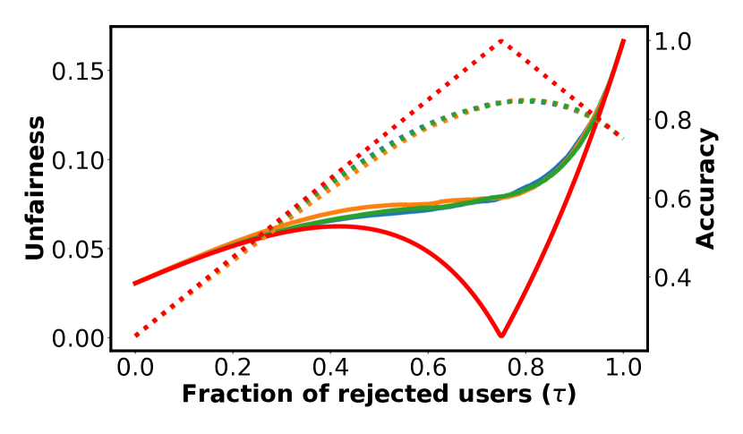
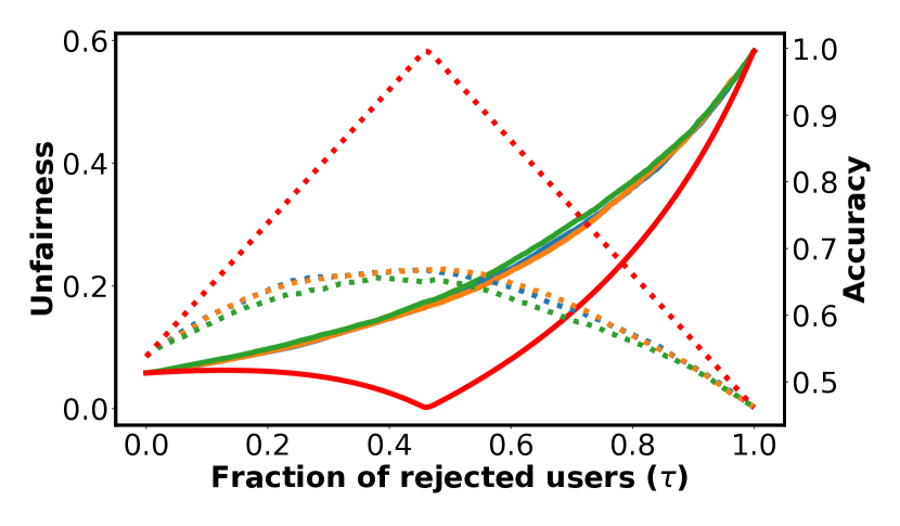
(a) Adult dataset

(b) COMPAS dataset

Figure 5. Overall unfairness (solid lines—$\mathcal{E}^{2}(\mathbf{b})$ in Eq. 5) and accuracy (dotted lines) as a function of the decision ranking threshold ($\mathbf{\tau}$) for various classifiers. The positive and negative class ratio in the Adult dataset is about $0.25:0.75$, hence the $1.00$ accuracy point corresponds to $\tau=0.75$. Similarly, the positive and negative class ratio in the COMPAS dataset is about $0.55:0.45$, hence the $1.00$ accuracy point corresponds to $\tau=0.45$. For oracle, the optimal point for accuracy corresponds to minimal unfairness; this doesn’t hold for other classifiers.

Setup and Datasets. We use the Generalized Entropy index (cf. Eq. 2) with $\alpha=2$ (in other words, half the squared coefficient of variation) to measure unfairness:

$$\mathcal{E}^{2}(b_{1},b_{2},\cdots,b_{n})=\frac{1}{2\times n}\sum_{i=1}^{n}\left[\left(\frac{b_{i}}{\mu}\right)^{2}-1\right].$$

As noted in Section 2, the Generalized Entropy index can be further decomposed into between-group and within-group unfairness as:

(5) $$\mathcal{E}^{2}(b_{1},b_{2},\cdots,b_{n})= \mathcal{E}^{2}_{\omega}(\mathbf{b})+\mathcal{E}^{2}_{\beta}(\mathbf{b}).$$

We will refer to the quantity $\mathcal{E}^{2}$ as individual unfairness or overall unfairness interchangeably, $\mathcal{E}^{2}_{\beta}$ as between-group unfairness, and $\mathcal{E}^{2}_{\omega}$ as within-group unfairness.

We experiment with two real-world datasets: (i) the Adult income dataset (Lichman, 2013), and (ii) the ProPublica COMPAS dataset (Larson et al., 2016). Both datasets have received previous attention (Zafar et al., 2017b, a; Corbett-Davies et al., 2017; Zemel et al., 2013; Feldman et al., 2015).

For the Adult income dataset, the task is to predict whether an individual earns more (positive class) or less (negative class) than 50,000 USD per year based on features like education level and occupation. We consider gender (female and male) and race (Black, White and Asian) as sensitive features. We filter out races (American Indian and Other) which constitute less than $1\%$ of the dataset. After the filtering, the dataset consists of $44,434$ subjects and $11$ features.

For the ProPublica COMPAS dataset, the task is to predict whether (negative class) or not (positive class) a criminal defendant would commit a crime within two years based on features like current charge degree or number of prior offenses. We use the same set of features as Zafar et al. (Zafar et al., 2017a). The sensitive features in this case are also gender (female and male) and race (Black, Hispanic, White). The dataset consists of $5,786$ subjects and $5$ features.

For all experiments, we repeatedly split the data into $70\%$-$30\%$ train-test sets 10 times and report average statistics. All hyperparameters are validated using a further $70\%$-$30\%$ split of the train set into train and validation sets.

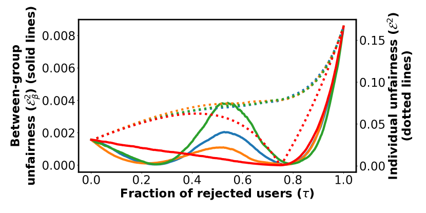
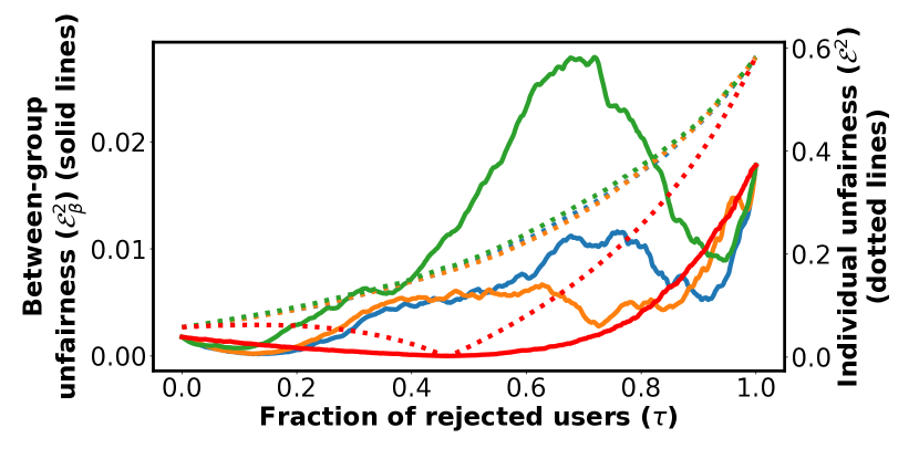
(a) Adult dataset

(b) COMPAS dataset

Figure 7. Between-group unfairness (solid lines—$\mathcal{E}^{2}_{\beta}(\mathbf{b})$ in Eq. 5) and overall unfairness (dotted lines—$\mathcal{E}^{2}(\mathbf{b})$ in Eq. 5) as a function of the decision ranking threshold ($\mathbf{\tau}$) for various classifiers. Between-group unfairness $\mathcal{E}^{2}_{\beta}(\mathbf{b})$ only constitutes a small fraction of the overall unfairness $\mathcal{E}^{2}(\mathbf{b})$.

4.1. Fairness vs. Accuracy Tradeoffs

We begin by studying the tradeoff between the accuracy and the overall individual unfairness of a given classifier ($\mathcal{E}^{2}(\mathbf{b})$ in Eq. 5). We use three standard classifier models: logistic regression, support vector machine with RBF kernel (SVM), and random forest classifier. Results in Section 4.1 and Section 4.2 are computed by optimizing these classifiers for accuracy.

Each of the above models computes the likelihood of belonging to the positive class for every instance. We denote this likelihood by $p_{i}$ for an individual $i$. We compare the fairness and accuracy of these classifiers with that of an “oracle” that can perfectly predict the label for every instance (and assigns $p_{i}\in\{0,1\}$). To predict a label in $\{0,1\}$ for individuals, we first rank all instances (in increasing order) according to their $p_{i}$ values with ties broken randomly; then we designate a decision ranking threshold $0\leq\tau\leq 1$ and output a label of $1$ for individual $i$ if and only if $rank(i)\geq n\tau$, where $rank(i)$ denotes the rank of individual $i$ in the sorted list. In other words, an increasing value of $\tau$ corresponds to the classifier rejecting more people from the sorted list (in order of their positive class likelihood $p_{i}$). As we vary $\tau$, we expect both accuracy as well as unfairness of the resulting predictions to change as discussed below and shown in Figure 5.

For the oracle, as expected from Proposition 3.1, a perfect accuracy corresponds to zero unfairness: with an increasing $\tau$, the accuracy increases while the unfairness decreases. After a certain optimal value of threshold $\tau$ (close to $0.75$ in the Adult data and $0.45$ in the COMPAS data), the trend reverses. We note that $0.75$ and $0.45$ represent the fraction of instances in the negative class in the respective datasets. Hence, at these optimal thresholds, all of the oracle’s predictions are accurate (since the points are ranked based on their positive class likelihood) resulting in $0$ unfairness.

However, for all other (non-oracle) classifiers, as expected via Proposition 3.2, the trend is very different: the optimal threshold for (imperfect) accuracy is far from the optimal threshold for unfairness. Moreover, with increasing $\tau$, while unfairness continually increases, for accuracy we initially see an increase followed by a drop. We note that the overall unfairness is not always a monotone function of the decision ranking threshold as illustrated in Example A.1.

4.2. Fairness Decomposability

As Figure 3 and Eq. 5 show, the individual unfairness of a predictor can be decomposed into between-group and within-group unfairness. In this part, we study the between-group unfairness component ($\mathcal{E}^{2}_{\beta}(\mathbf{b})$ in Eq. 5) as we change $\tau$. To this end, we consider two sensitive features: gender and race. We split each of the datasets into all possible disjoint groups based on these sensitive features (e.g., White women, Hispanic men, Black women).

Figure 7 shows between-group unfairness along with overall unfairness for different values of $\tau$. We notice that for the Adult dataset, the between-group unfairness follows a multi-modal trend: it starts from a non-zero value at $\tau=0$, falls to almost $0$ for most classifiers (except for the oracle) at around $\tau=0.2$, reaches a local peak again around $\tau=0.5$, and finally completes another cycle to fall and then reach its maximum value at $\tau=1.0$. The COMPAS dataset also shows a similar trend, albeit to a lesser extent.

Between-group unfairness and overall unfairness. Comparing the between-group unfairness and overall unfairness in Figure 7 reveals a very interesting insight: for the same value of $\tau$, the between-group unfairness (solid lines) is a very small fraction of the overall unfairness (dotted lines). For example, considering the performance of the logistic regression classifier on the COMPAS dataset, the maximum value of the overall unfairness is close to $0.6$ whereas the maximum value of the between-group unfairness is merely $0.01$. We hypothesize that since the number of sensitive feature-based groups is much smaller than the number of all individuals in the dataset, the individual unfairness value dominates the between-group unfairness.

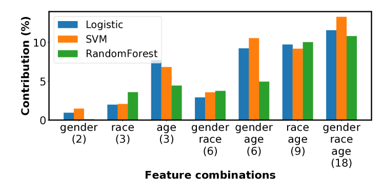
Figure 8. Between-group unfairness ($\mathcal{E}^{2}_{\beta}(\mathbf{b})$ in Eq. 5) as a fraction of the overall/individual unfairness ($\mathcal{E}^{2}(\mathbf{b})$ in Eq. 5) for various combinations of sensitive features. Numbers on the x-axis denote how many sensitive feature groups would be formed when using the corresponding sensitive feature set. Logistic regression, SVM and Random Forests achieve similar accuracies of 66%, 67% and 65% as well as similar overall individual unfairness of 0.145, 0.151 and 0.134 respectively on the ProPublica Compas dataset.

Between-group

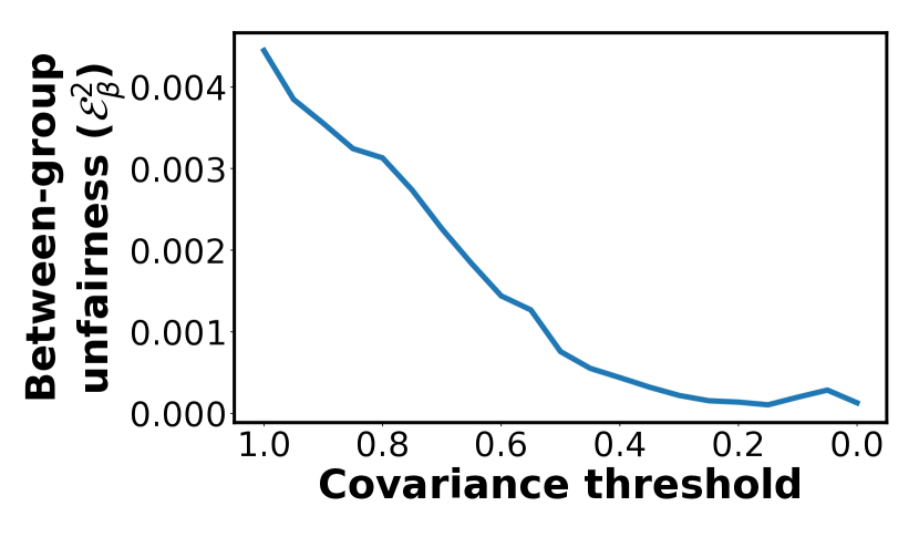
Within-group

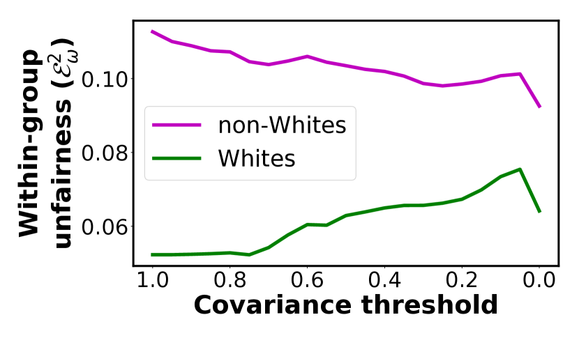
Overall / individual

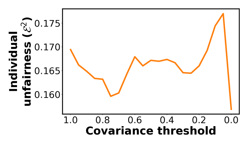
Figure 10. The effect of applying false negative rate constraints of Zafar et al. in order to minimize the between-group unfairness ($\mathcal{E}^{2}_{\beta}(\mathbf{b})$). The second plot shows that reducing the between-group unfairness leads to an increase in the within-group unfairness ($\mathcal{E}^{2}_{\omega}(\mathbf{b})$) for Whites. Moreover, for certain values of the covariance threshold, the overall unfairness ($\mathcal{E}^{2}(\mathbf{b})$) increases as compared to the unconstrained classifier.

To test this hypothesis, we experiment with the following setup: We take the three sensitive features present in the COMPAS dataset, namely gender, race and age, and form sensitive feature groups based on all possible combinations of these features. For example, groups formed based on gender would be men and women; groups formed based on race would be Black, White and Hispanic; whereas groups formed based on gender as well as race would be Black men, Black women, White men and so on. For each of these sensitive feature combinations we plot in Figure 8 the percentage of contribution that the between-group unfairness has towards the overall unfairness. Figure 8 shows that as the number of sensitive feature groups increases, the between-group unfairness contributes more and more towards the overall unfairness. This result is also in line with the implications of Proposition 3.4.

Figure 8 also shows the following interesting insight: Even though the overall unfairness and accuracy of all the classifiers is very similar (cf. Figure 5), the random forest classifier leads of significantly smaller contribution of between-group unfairness as compared to other classifier (e.g., gender, gender+age). In other words even for similar levels of accuracy and overall unfairness, classifiers have very different between-group unfairness across different feature sets.

Accuracy and between-group unfairness. We also study the between group unfairness in Figure 7 and corresponding accuracy in Figure 5. We notice that there is no definitive correlation between the accuracy and the between-group unfairness: In the Adult dataset, the highest level of accuracy (around $\tau=0.8$) corresponds to one of the lowest values of between-group unfairness for all classifiers. However, this doesn’t hold in the case of COMPAS dataset.

4.3. Interaction Between Different Types of Unfairness

In this section, we revisit the literature on fairness-aware machine learning and investigate how methods proposed to control between-group unfairness (which is what most existing methods focus on (Zafar et al., 2017b, a; Feldman et al., 2015; Kamiran and Calders, 2009; Kamishima et al., 2013; Zemel et al., 2013; Hardt et al., 2016)) can affect the overall/individual and the within-group unfairness. Specifically, we study how the overall unfairness ($\mathcal{E}^{2}(\mathbf{b})$ in Eq. 5) and the within-group unfairness ($\mathcal{E}^{2}_{\omega}(\mathbf{b})$ in Eq. 5) would change when training a constrained classifier to minimize the between-group unfairness ($\mathcal{E}^{2}_{\beta}(\mathbf{b})$ in Eq. 5). Our study is motivated by the fact that while several methods focus on designing constraints to remove the between-group unfairness (e.g., see (Zafar et al., 2017a; Hardt et al., 2016; Zemel et al., 2013)), to the best of our knowledge, no prior work in fairness-aware machine learning has studied the effect of these constraints on the overall and the within-group unfairness.

To this end, we use the methodology proposed by Zafar et al. (Zafar et al., 2017a) to remove the between-group unfairness based on false negative rates between different races (Whites and non-Whites) in the COMPAS dataset. Zafar et al. propose to remove the between-group unfairness by bounding the covariance between misclassification distance from the decision boundary and the sensitive feature value. The method operates by bounding the covariance of the unconstrained classifier by successive multiplicative factors between 1 and 0. A covariance multiplicative factor of $1$ means that no fairness constraints are applied while training the classifier, whereas a factor of $0$ means the tightest possible constraints are applied. As done by Zafar et al., we train several logistic regression classifiers to limit the between-group unfairness; each classifier is trained with a covariance multiplicative factor in the range $[1.00,0.95,0.90,\ldots,0.05,0.00]$.

Figure 10 shows the between-group unfairness, within-group unfairness, and overall/individual unfairness as the fairness constraints of Zafar et al. (Zafar et al., 2017a) are tightened towards $0$. The figure shows the following key insights: (i) Reducing the between-group unfairness can in fact increase the within-group unfairness: the within-group unfairness for Whites almost monotonically increases as the between-group unfairness is reduced. This observation also follows Proposition 3.3. (ii) Reducing the between-group unfairness can exacerbate overall/individual unfairness: As the between-group unfairness decreases between the covariance multiplicative factor of $0.8$ to $0.6$ (on the x-axis), the overall unfairness in fact goes up. These insights point to possible significant tensions between these different components of unfairness.

Summary of empirical analysis. Experiments on multiple real-world datasets performed in this section support the theoretical analysis of Section 3. The empirical (as well as the theoretical) analysis brings out the inherent tensions between fairness and accuracy, as well as between different (between- and within-group) components of fairness. These results point to potential for situations where optimizing for one type of fairness can exacerbate the other.

5. Conclusion

We proposed using inequality indices from economics as a principled way to compute the scalar degree of total unfairness of any algorithmic decision system. The approach is based on well-justified principles (axioms), and is general enough so that by varying the benefit function, we can capture all previous notions of algorithmic fairness conditions as special cases, while also admitting interesting generalizations. The resulting measures of total unfairness unify previous concepts of group and individual fairness, and allow us to study quantitatively the behavior of earlier methods to mitigate unfairness. These earlier methods typically worry only about between-group unfairness, which may be justified for legal reasons, or in order to redress particular social prejudices. However, we demonstrate that minimizing exclusively between-group unfairness may actually increase overall unfairness.

Appendix A Appendix: Technical Material

Proof of Proposition 3.1

If there exists a classifier $\theta^{\prime}$ with $L_{\mathcal{D}}(\theta^{\prime})=0$, then that classifier minimizes $I$: For all $i=1,\cdots,n$, the benefit $i$ receives under $\theta^{\prime}$, denoted by $b^{\theta^{\prime}}_{i}$, is equal to $1+\theta^{\prime}(\mathbf{x}_{i})-y_{i}=1$. That is everyone gets the same benefit under $\theta^{\prime}$, and as the result, $I(\mathbf{b}^{\theta^{\prime}})=I(\mathbf{1})=0$.

If there exists a classifier $\theta$ with $I(\mathbf{b}^{\theta})=0$, $\theta$ must assign the same benefit to everyone: there exists $b\in\{0,1,2\}$ such that for all $i=1,\cdots,n$, $b^{\theta}_{i}=1+\theta(\mathbf{x}_{i})-y_{i}=b$. Now let $\theta^{\prime}(\mathbf{x})=\theta(\mathbf{x})+1-b$. It is easy to verify that $\theta^{\prime}$ has zero error (i.e. $L_{\mathcal{D}}(\theta^{\prime})=0$). ∎

Proof of Proposition 3.2

Let $p=\mathbb{P}_{(\mathbf{x},y)\sim\mathcal{P}}[y=1|\mathbf{x}=\tilde{\mathbf{x}}]$ so that $0<p<0.5$. We know that the Bayes/accuracy optimal classifier assigns label 0 to every instance $i$ with $\mathbf{x}_{i}=\tilde{\mathbf{x}}$. Suppose $\mathcal{D}$ consists of $n$ instances all with $\mathbf{x}_{i}=\tilde{\mathbf{x}}$. Given the population invariance property of $I$, $n$ can be arbitrarily large without affecting the value of $I(.)$. Therefore we instead reason about the limiting case where $n=\infty$. In this case, we expect exactly $p$ fraction of the instances to have $y=1$ and the other $(1-p)$ fraction to have $y=0$. The benefit distribution $\mathbf{b}^{A}$ for $\theta^{A}$, therefore, consists of $p$ fraction of the population receiving benefit $0$ and the other $(1-p)$ fraction receiving $1$.

Now consider a probabilistic classifier $\theta^{q}$ that randomly assigns label 1 to each instance in $\mathcal{D}$ with probability $q\in(0,1)$. The resulting benefit distribution $\mathbf{b}^{q}$ of $\theta^{q}$ is as follows: $p(1-q)$ fraction of the population receive benefit $0$; $pq+(1-p)(1-q)$ faction receive benefit $1$; and $(1-p)q$ faction receive benefit $2$.

We claim that for $q=(1-p)$, $I_{\mathcal{D}}(\theta^{A})>I_{\mathcal{D}}(\theta^{q})$. To see this, note that $\mathbf{b}^{q}$ can be constructed from $\mathbf{b}^{A}$ via a series of inequality-reducing operations:

1. $\mathbf{b}^{\prime}=2\times\mathbf{b}^{A}$, so that $\mathbf{b}^{\prime}$ consists of $p$ fraction of the population receiving benefit $0$ and the other $(1-p)$ fraction receiving $2$. Due to the scale invariance property of $I$, we know $I(\mathbf{b}^{\prime})=I(\mathbf{b}^{A})$.

2. Perform the following progressive transfer on $\mathbf{b}^{\prime}$ to obtain $\mathbf{b}^{\prime\prime}$: Take one unit of benefit from $p(1-p)$ fraction of the population whose benefit is 2, and give it to $p(1-p)$ fraction with benefit 0. The resulting distribution, $\mathbf{b}^{\prime\prime}$, consists of $p^{2}$ faction with benefit $0$; $2p(1-p)$ faction with benefit $1$; and $(1-p)^{2}$ faction with benefit $2$. Because $I$ satisfies the Dalton principle and $p(1-p)>0$, we have that $I(\mathbf{b}^{\prime\prime})<I(\mathbf{b}^{\prime})$.

Combining the above two, we have $I(\mathbf{b}^{\prime\prime})<I(\mathbf{b}^{A})$. It only remains to note that $\mathbf{b}^{\prime\prime}$ is precisely $\mathbf{b}^{q}$ for $q=(1-p)$. Therefore, we conclude $I(\mathbf{b}^{\prime\prime})=I(\mathbf{b}^{(1-p)})<I(\mathbf{b}^{A})$. This finishes the proof. ∎

The following example shows that the accuracy of the fairness optimal classifier can be arbitrarily bad compared to that of the accuracy optimal classifier.

Example A.1.

Consider the example in the proof of Proposition 3.2. Let $I$ be the generalized entropy with $\alpha=2$. We claim that the fairness optimal classifier is one that assigns label 1 to every instance. To see this, recall that under $\theta^{q}$, $p(1-q)$ fraction of the population receive benefit $0$; $pq+(1-p)(1-q)$ faction receive benefit $1$; and $(1-p)q$ faction receive benefit $2$. So the mean benefit $\mu$ is equal to $1-p+q$. Taking derivative with respect to $q$, we have

$$\frac{d}{dq}\left((pq+(1-p)(1-q))\left(\frac{1}{1-p+q}\right)^{2}+(1-p)q\left(\frac{2}{1-p+q}\right)^{2}\right)=0$$

$$\Rightarrow q^{*}=\frac{1-3p+2p^{2}}{3-2p}$$

The derivative is positive for $q<q^{*}$ and negative for $q>q^{*}$. The minimum therefore happens at either $q=0$ or $q=1$. Given that for $0<p<1$, $\frac{1}{1-p}>\frac{4-3p}{(2-p)^{2}}$, we obtain that $q=1$ minimizes $I$.

The fairness optimal classifier assigns label 1 to every instance resulting in accuracy $p$, whereas the accuracy optimal classifier can achieve accuracy $(1-p)$. The ratio $\frac{1-p}{p}$ can be arbitrarily large if $p$ is taken to be sufficiently small.

Proof of Proposition 3.3

Note that because of the optimality of $\theta^{*}_{\beta}$ for (4), if $I_{\beta}(\theta^{*}_{\beta})\neq I_{\beta}(\theta^{*})$, it must be the case that $I_{\beta}(\theta^{*}_{\beta})<I_{\beta}(\theta^{*})$. If $I(\theta^{*}_{\beta})\leq I(\theta^{*})$, then $\theta^{*}_{\beta}$ is an optimal solution to (3), and $I_{\beta}(\theta^{*}_{\beta})<I_{\beta}(\theta^{*})$. This is a contradiction with the choice of $\theta^{*}$. If $I_{\omega}(\theta^{*}_{\beta})\leq I_{\omega}(\theta^{*})$, then combined with the fact that $I_{\beta}(\theta^{*}_{\beta})<I_{\beta}(\theta^{*})$, we have that $I(\theta^{*}_{\beta})<I(\theta^{*})$, which is a contradiction with the optimality of $\theta^{*}$ for (3). ∎

Proof of Proposition 3.4

Suppose $|G|=m$ and $|G^{\prime}|=m^{\prime}.$ Let $\mathbf{b}=\left(\mathbf{b}^{(g_{1},g^{\prime}_{1})},\cdots,\mathbf{b}^{(g_{m},g^{\prime}_{m^{\prime}})}\right)$ where $\mathbf{b}^{(g_{i},g^{\prime}_{j})}$ specifies the benefit distribution for individuals in group $(g_{i},g^{\prime}_{j})$ and $\boldsymbol{\mu}^{(g_{i},g^{\prime}_{j})}$ specifies the distribution in which each individual in $(g_{i},g^{\prime}_{j})$ receives the group’s mean benefit. Note that $I^{G\times G^{\prime}}_{\beta}(\mathbf{b})$ can be written as

$$I\left(\boldsymbol{\mu}^{(g_{1},g^{\prime}_{1})},\cdots,\boldsymbol{\mu}^{(g_{m},g^{\prime}_{m^{\prime}})}\right)$$

$$= I^{G}_{\beta}\left(\boldsymbol{\mu}^{(g_{1},g^{\prime}_{1})},\cdots,\boldsymbol{\mu}^{(g_{m},g^{\prime}_{m^{\prime}})}\right)+I^{G}_{\omega}\left(\boldsymbol{\mu}^{(g_{1},g^{\prime}_{1})},\cdots,\boldsymbol{\mu}^{(g_{m},g^{\prime}_{m^{\prime}})}\right)$$

$$= I\left(\boldsymbol{\mu}^{g_{1}},\cdots,\boldsymbol{\mu}^{g_{m}}\right)+I^{G}_{\omega}\left(\boldsymbol{\mu}^{(g_{1},g^{\prime}_{1})},\cdots,\boldsymbol{\mu}^{(g_{m},g^{\prime}_{m^{\prime}})}\right)$$

$$\geq I\left(\boldsymbol{\mu}^{g_{1}},\cdots,\boldsymbol{\mu}^{g_{m}}\right)$$

$$= I^{G}_{\beta}(\mathbf{b})$$

where to obtain the second line, we used the additive decomposability property of $I$; for the third line we used the definition of the between-group component, and finally to obtain the conclusion, we used the zero-normalization property of $I$. ∎

Proof of Proposition 3.5

Recall that $I(\mathbf{b})=I^{G}_{\beta}(\mathbf{b})+I^{G}_{\omega}(\mathbf{b})$ and $I^{G}_{\beta}(\mathbf{b}),I^{G}_{\omega}(\mathbf{b})\geq 0$. Therefore, we have $0\leq\frac{I^{G}_{\beta}(\mathbf{b})}{I(\mathbf{b})}\leq 1$.

Consider a benefit distribution $\mathbf{b}$ in which members of group $g_{1}\in G$ receive benefit 1, and everyone else receives benefit $0$. It is easy to see that for this distribution $\frac{I^{G}_{\beta}(\mathbf{b})}{I(\mathbf{b})}=1$. Similarly, consider a benefit distribution $\mathbf{b}^{\prime}$ that assigns a benefit of 1 to half of the population in each group, and 0 to everyone else. It is easy to that $\frac{I^{G}_{\beta}(\mathbf{b}^{\prime})}{I(\mathbf{b}^{\prime})}=0$. ∎

The following example shows that an added feature may in fact worsen the unfairness of the accuracy optimal classifier.

Example A.2.

Let $I(.)$ be the generalized entropy with $\alpha=2$. Suppose for all $\mathbf{x}_{i}=\tilde{\mathbf{x}}$, $p=\mathbb{P}_{(\mathbf{x},y)\sim D}[y=1|\mathbf{x}=\tilde{\mathbf{x}}]>0.5$, so $\theta^{A}$ assigns label 1 to every instance with $\mathbf{x}_{i}=\tilde{\mathbf{x}}$. So in the resulting benefit distribution, $p$ fraction of the population receives benefit $1$ and the other $(1-p)$ fraction receives $2$. The mean benefit is, therefore, $(2-p)$ and GE is equal to

$$p\left(\frac{1}{2-p}\right)^{2}+(1-p)\left(\frac{2}{2-p}\right)^{2}=\frac{4-3p}{(2-p)^{2}}.$$

Suppose with the addition of a new binary feature, the population breaks down into two subpopulations, one corresponding to $\mathbf{x}=(\tilde{\mathbf{x}},0)$ and the other corresponding to $\mathbf{x}=(\tilde{\mathbf{x}},1)$. Let $\frac{r}{1-r}$ be the relative size of the former sub-population to the latter ($0\leq r\leq 1$). We would like the accuracy optimal classifier to be different for each subpopulation, so for now let’s assume:

• $\mathbb{P}_{(\mathbf{x},y)\sim D}[y=1\wedge\mathbf{x}=(\tilde{\mathbf{x}},0)]=\frac{r}{2}-\epsilon$, so $\theta^{A}$ assigns label 0 to every instance with $\mathbf{x}=(\tilde{\mathbf{x}},0)$—this is because $\frac{r}{2}-\epsilon<\frac{1}{2}r$.

• $\mathbb{P}_{(\mathbf{x},y)\sim D}[y=1\wedge\mathbf{x}=(\tilde{\mathbf{x}},1)]=p-\frac{r}{2}+\epsilon$, so $\theta^{A}$ assigns label 1 to every instance with $\mathbf{x}=(\tilde{\mathbf{x}},1)$—this is because $p-\frac{r}{2}+\epsilon>\frac{1}{2}(1-r)$.

In the resulting benefit distribution, $\frac{r}{2}-\epsilon$ fraction of the total population receives benefit $0$, $p+2\epsilon$ fraction of the total population receives benefit $1$, and the other $(1-p-\frac{r}{2}-\epsilon)$ fraction receives benefit $2$. The mean benefit is, therefore, $(2-p-r)$ and GE is equal to

$$(p+2\epsilon)\left(\frac{1}{2-p-r}\right)^{2}+(1-p-\frac{r}{2}-\epsilon)\left(\frac{2}{2-p-r}\right)^{2}$$

$$=\frac{4-3p-2r-2\epsilon}{(2-p-r)^{2}}.$$

Take $p=0.9$, $r=0.2$ and $\epsilon=0.001$, and we have:

$$\frac{4-3p}{(2-p)^{2}}=1.075$$

$$\frac{4-3p-2r-2\epsilon}{(2-p-r)^{2}}=1.10$$

The above shows the addition of a new feature can worsen the fairness of the accuracy optimal classifier.

References

- (1)
- Abdi (2010) Hervé Abdi. 2010. Coefficient of variation. Encyclopedia of research design 1 (2010), 169–171.
- Angwin et al. (2016) Julia Angwin, Jeff Larson, Surya Mattu, and Lauren Kirchner. 2016. Machine Bias: There’s Software Used Across the Country to Predict Future Criminals. And it’s Biased Against Blacks. https://www.propublica.org/article/machine-bias-risk-assessments-in-criminal-sentencing.
- Atkinson (1970) Anthony B. Atkinson. 1970. On the measurement of inequality. Journal of economic theory 2, 3 (1970), 244–263.
- Barocas and Selbst (2016) Solon Barocas and Andrew D Selbst. 2016. Big data’s disparate impact. California Law Review 104 (2016), 671.
- Bellù and Liberati (2006) Lorenzo Giovanni Bellù and Paolo Liberati. 2006. Inequality analysis: The gini index. Food and Agriculture Organization of the United Nations, EASYPol Module 40 (2006).
- Berk et al. (2017) Richard Berk, Hoda Heidari, Shahin Jabbari, Michael Kearns, and Aaron Roth. 2017. Fairness in criminal justice risk assessments: The state of the art. arXiv preprint arXiv:1703.09207 (2017).
- Chouldechova (2016) Alexandra Chouldechova. 2016. Fair Prediction with Disparate Impact: A Study of Bias in Recidivism Prediction Instruments. arXiv:1610.07524 (2016).
- Conceição and Ferreira (2000) Pedro Conceição and Pedro Ferreira. 2000. The young person’s guide to the Theil index: Suggesting intuitive interpretations and exploring analytical applications. (2000).
- Corbett-Davies et al. (2017) Sam Corbett-Davies, Emma Pierson, Avi Feller, Sharad Goel, and Aziz Huq. 2017. Algorithmic decision making and the cost of fairness. In Proceedings of KDD.
- Cowell and Kuga (1981) Frank A. Cowell and Kiyoshi Kuga. 1981. Additivity and the entropy concept: an axiomatic approach to inequality measurement. Journal of Economic Theory 25, 1 (1981), 131–143.
- Dalton (1920) Hugh Dalton. 1920. The measurement of the inequality of incomes. The Economic Journal 30, 119 (1920), 348–361.
- Dwork et al. (2012) Cynthia Dwork, Moritz Hardt, Toniann Pitassi, Omer Reingold, and Richard Zemel. 2012. Fairness through awareness. In Proceedings of the 3rd Innovations in Theoretical Computer Science Conference (ITCS). 214–226.
- Feldman et al. (2015) Michael Feldman, Sorelle A. Friedler, John Moeller, Carlos Scheidegger, and Suresh Venkatasubramanian. 2015. Certifying and Removing Disparate Impact. In Proceedings of KDD.
- Flores et al. (2016) Anthony W. Flores, Christopher T. Lowenkamp, and Kristin Bechtel. 2016. False Positives, False Negatives, and False Analyses: A Rejoinder to "Machine Bias: There’s Software Used Across the Country to Predict Future Criminals. And it’s Biased Against Blacks.". (2016).
- Furletti (2002) Mark J. Furletti. 2002. An Overview and History of Credit Reporting. http://dx.doi.org/10.2139/ssrn.927487.
- Gini (1912) Corrado Gini. 1912. Variabilità e mutabilità. Reprinted in Memorie di metodologica statistica (Ed. Pizetti E, Salvemini, T). Rome: Libreria Eredi Virgilio Veschi (1912).
- Hardt et al. (2016) Moritz Hardt, Eric Price, Nati Srebro, et al. 2016. Equality of opportunity in supervised learning. In Proceedings of NIPS. 3315–3323.
- Joseph et al. (2016) Matthew Joseph, Michael Kearns, Jamie Morgenstern, and Aaron Roth. 2016. Fairness in learning: Classic and contextual bandits. In Proceedings of NIPS. 325–333.
- Kakwani (1980) Nanak Kakwani. 1980. On a class of poverty measures. Econometrica: Journal of the Econometric Society (1980), 437–446.
- Kamiran and Calders (2009) Faisal Kamiran and Toon Calders. 2009. Classifying without discriminating. In Proceedings of the 2nd International Conference on Computer, Control and Communication. IEEE, 1–6.
- Kamishima et al. (2013) Toshihiro Kamishima, Shotaro Akaho, and Jun Sakuma. 2013. Efficiency improvement of neutrality-enhanced recommendation. In RecSys.
- Kearns et al. (2017) Michael Kearns, Seth Neel, Aaron Roth, and Zhiwei Steven Wu. 2017. Preventing fairness gerrymandering: Auditing and learning for subgroup fairness. arXiv preprint arXiv:1711.05144 (2017).
- Kleinberg et al. (2017) Jon Kleinberg, Sendhil Mullainathan, and Manish Raghavan. 2017. Inherent Trade-Offs in the Fair Determination of Risk Scores. In Proceedings of ITCS.
- Kolm (1976a) Serge-Christophe Kolm. 1976a. Unequal inequalities. I. Journal of economic Theory 12, 3 (1976), 416–442.
- Kolm (1976b) Serge-Christophe Kolm. 1976b. Unequal inequalities. II. Journal of Economic Theory 13, 1 (1976), 82–111.
- Larson et al. (2016) Jeff Larson, Surya Mattu, Lauren Kirchner, and Julia Angwin. 2016. Data and analysis for ‘How we analyzed the COMPAS recidivism algorithm’. https://github.com/propublica/compas-analysis.
- Lichman (2013) M. Lichman. 2013. UCI machine learning repository: The Adult income data set. https://archive.ics.uci.edu/ml/datasets/adult.
- Litchfield (1999) Julie A. Litchfield. 1999. Inequality: Methods and tools. World Bank 4 (1999).
- Long and Nucci (1997) Larry Long and Alfred Nucci. 1997. The Hoover index of population concentration: A correction and update. The Professional Geographer (1997).
- Lundberg and Lee (2017) Scott M. Lundberg and Su-In Lee. 2017. A unified approach to interpreting model predictions. In Proceedings of NIPS. 4768–4777.
- Pigou (1912) Arthur Cecil Pigou. 1912. Wealth and welfare. Macmillan and Company, limited.
- Podesta et al. (2014) John Podesta, Penny Pritzker, Ernest Moniz, John Holdren, and Jeffrey Zients. 2014. Big data: Seizing opportunities, preserving values. Executive Office of the President. The White House. (2014).
- Romei and Ruggieri (2014) Andrea Romei and Salvatore Ruggieri. 2014. A multidisciplinary survey on discrimination analysis. The Knowledge Engineering Review 29, 5 (2014), 582–638.
- Sen (1973) Amartya Sen. 1973. On economic inequality. Oxford University Press.
- Shorrocks (1980) Anthony F Shorrocks. 1980. The class of additively decomposable inequality measures. Econometrica: Journal of the Econometric Society (1980), 613–625.
- Subramanian (2011) Subbu Subramanian. 2011. Inequality measurement with subgroup decomposability and level-sensitivity. (2011).
- Summers and Willis (2010) Charles Summers and Tim Willis. 2010. Pretrial risk assessment.
- Sundararajan et al. (2017) Mukund Sundararajan, Ankur Taly, and Qiqi Yan. 2017. Axiomatic Attribution for Deep Networks. In Proceedings of ICML. 3319–3328.
- Theil (1967) Henri Theil. 1967. Economics and Information Theory. North Holland, Amsterdam.
- Zafar et al. (2017a) Muhammad Bilal Zafar, Isabel Valera, Manuel Gomez Rodriguez, and Krishna P. Gummadi. 2017a. Fairness beyond disparate treatment & disparate impact: Learning classification without disparate mistreatment. In In proceedings of WWW.
- Zafar et al. (2017b) Muhammad Bilal Zafar, Isabel Valera, Manuel Gomez Rodriguez, and Krishna P. Gummadi. 2017b. Fairness constraints: Mechanisms for fair classification. In Proceedings of AISTATS.
- Zemel et al. (2013) Rich Zemel, Yu Wu, Kevin Swersky, Toni Pitassi, and Cynthia Dwork. 2013. Learning fair representations. In Proceedings of ICML. 325–333.